Embed Size (px)
Citation preview

Biophysical Model Building
1
• Step 1: Come up with a hypothesis about how a system works– How many binding sites?– Is there cooperativity?
• Step 2: Translate the qualitative hypotheses into an observable mathematical form with parameters– Example parameters: K, tau, N– Parameters may not be known
• Step 3: Design an experiment that that can produce observables from step 2; perform the experiment– Optimize the parameters to make the fit look as good as possible
• Step 4: Assess the fit – Is the agreement convincing?

Example: Single Site Binding
2
• Situation: You are studying a novel DNA‐binding protein
• Hypothesis: – Parameters: K– Implicitly, we assume that N = 1, no cooperativity
• Experiment: Collect a binding curve (dialysis)– Optimize K for the best fit
• Assess: How good is our fit? Use statistics!

Example: Single Site Binding
3
• Situation: You are studying a novel DNA‐binding protein
• Hypothesis: – Parameters: K– Implicitly, we assume that N = 1, no cooperativity
• Experiment: Collect a binding curve (dialysis)– Optimize K for the best fit
• Assess: How good is our fit? Use statistics!
What about the Thermodynamics?
• Free energies:Δ ̅ ln
• Enthalpies: Van’t Hoff
lnΔ 1 1
• Once the appropriate thermodynamic variables are known, one can predict K at any T, P, etc.

Helix‐Coil Theory
4
• Question: How does an α‐helix fold?Hi Oi‐3

Helix‐Coil Theory: Considerations
5
• Entropic cost: 3 pairs of φ, ψ torsions must be “fixed” before 1 hydrogen bond is formed
• Energetic benefit: forming H‐bond is favorable once torsions are “fixed”
• End effects: No H‐bonds for the end residues
Hi Oi‐3

Helix‐Coil Theory: Assumptions
6
• Assumption 1: Each residue can exist in one of two conformational states: h or c– h (helix) is one conformation, c (coil) represents many energetically equivalent conformations
– We can “enumerate” confirmations with a series of h’s and c’s
– For 8 residues:hhhhcccc ccchhccchchchchc hhhhhhhh

Helix‐Coil Theory: Assumptions
7
• Assumption 2: For any sequence we consider, assume it’s flanked by an infinite number of “coil” residues– This allows us to ignore end effects
ccchhccc …cccccchhcccccc…hhhhhhhh …ccchhhhhhhhccc…hhhhcccc …ccchhhhccccccc…

Helix‐Coil Theory: Assumptions
8
• Assumption 3: Assume some conformations are not observed– hch, hcch: helical kinks, but no energetic benefit
ccchhccc possiblehhhhhhhh possiblehchhhccc not possiblehhhcchhh not possiblehhccchhh possible

Helix‐Coil Theory: Assumptions
9
• Assumption 4a: Individual residues are in equilibrium– If a new helical residue tries to form at the end of an existing helix:
hhhccccc hhhhcccc

Helix‐Coil Theory: Assumptions
10
• Assumption 4b: Individual residues are in equilibrium– If a new helical residue tries to form “from scratch”:
cccccccc ccchcccc
– represents entropic cost of forming a helical φ, ψ values ( )

Helix‐Coil Theory: Assumptions
11
• Assumption 5: Let the “unfolded” (i.e. all‐coil) state be our reference state– Statistical weight of …cccccccc… = 1

Helix‐Coil Theory: So What?
12
• Make a table (for N = 3):State # Helical
ResiduesWeight
…ccc… 0 1
…hcc… 1 ?
…chc… 1 ?
…cch… 1 ?
…hhc… 2 ?
…hch… 2 ?
…chh… 2 ?
…hhh… 3 ?

Helix‐Coil Theory: So What?
13
• Make a table (for N = 3):State # Helical
ResiduesWeight
…ccc… 0 1
…hcc… 1
…chc… 1
…cch… 1
…hhc… 2 ?
…hch… 2 ?
…chh… 2 ?
…hhh… 3 ?
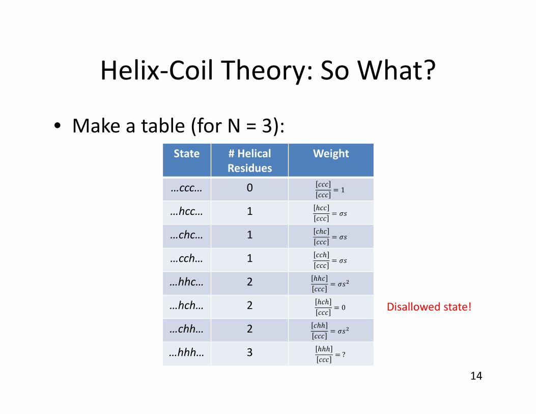
Helix‐Coil Theory: So What?
14
• Make a table (for N = 3):State # Helical
ResiduesWeight
…ccc… 0 1
…hcc… 1
…chc… 1
…cch… 1
…hhc… 2
…hch… 2 0
…chh… 2
…hhh… 3 ?
Disallowed state!

Helix‐Coil Theory: So What?
15
• Make a table (for N = 3):State # Helical
ResiduesWeight
…ccc… 0 1
…hcc… 1
…chc… 1
…cch… 1
…hhc… 2
…hch… 2 0
…chh… 2
…hhh… 3

Helix‐Coil Theory: Experiment
16
• Partition function:∑
1 3 2
• Weighted average # helical residues:
helix ∑
• <helix> is measurable!
State # HelicalResidues
Weight
…ccc… 0 1
…hcc… 1
…chc… 1
…cch… 1
…hhc… 2
…hch… 2 0
…chh… 2
…hhh… 3

Helix‐Coil Theory: Experiment
Tinoco, p. 175. 17
Helix‐Coil Theory: Takeaways
18
• Typical parameters– (sometimes favorable, sometimes unfavorable depending on the solvent hydrogen bond strength?
– (typically on the order 0.001) entropy is difficult to overcome
• Cooperativity comes from small σ relative to s
• It’s hard to break a helix in the middle– Helix typically “frays” at the ends

Helix‐Coil Theory: DNA?
19
• DNA is more complicated than protein– Different base pairs different s values– Two strands involved σ is concentration dependent
– Individual strands can “shift” relative to one another
• Lots of people have studied this (see book)

Random Walk in 1D
20
• Molecule diffuses (average distance) before colliding with another molecule– This is the “step size” per hop
• For one step, probability (weight) of traveling forward is , probability of traveling backward is

Random Walk for 3 Steps
21
• Partition function:∑
3 3
• Avg. # forward steps:m
∑
• Mean displacement:d
d 2
• When , d 0– Why?
Steps # ForwardSteps
Weight
fff 3bff 2fbf 2ffb 2bbf 1bfb 1fbb 1bbb 0

Random Walk
22
• Random walk in 1‐D can be solved in general for N steps (see p. 167‐172)
• Main point:When , the mean‐squared displacement is:
• This can be used to model the end‐to‐end distance of an unfolded chain with no self‐avoidance (N = # of links)

What Have We Learned?
23
• Many biological systems are made up of discrete states– Bound Free; Native Unfolded; Helix Coil
• If we can determine relative concentrations (weights), we can sum the weights to get a partition function
• Once we know weights and the partition function, we can calculate observable values– Mole fractions:
– Weighted averages: ∑
– Degree of binding: ̅ ∑

What Don’t We Know?
24
• Can we calculate weights directly from energy differences (i.e. )?
• Can we relate entropy to the number of possible states?
• What is the molecular significance of the partition function?

Generic Table of States
25
State Degeneracy Generic Energy mol‐1 Weight
1
2
3
… … … …
N
• Boltzmann Distribution gives mole fractions:/
• Partition function is defined like before:̅ /

Boltzmann Distribution: Implications
26
• If we know total molecules (Ntot), the number of molecules in state i (Ni):
/
• The fraction of molecules is simply/
• Total and average energy:∑ /

Work and Heat
27
• “Generic Energy” can be (binding), but if E is internal energy, we write:
• Derivation is pretty neat (p. 157‐158)– Adding heat changes distribution of states (dN)
Work Heat
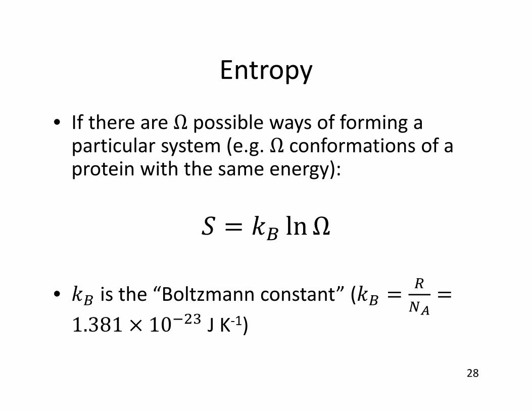
Entropy
28
• If there are possible ways of forming a particular system (e.g. conformations of a protein with the same energy):
• is the “Boltzmann constant” (J K‐1)

Partition Function
29
• The partition function (Z) can be related to U and S:
• Why is this important?– If we knew the partition function exactly (hard to do), we could predict equilibrium constants, etc.

Summary: Statistical Thermodynamics
30
• Tables of states What fraction of molecules is in each state– Statistics pertains to counting: how many x in y
• Partition function is the key to all systems we’ve discussed
• We’ve covered small numbers of discrete states (with discrete energies)– Large systems often have many more states and energies look continuous