Biosphere feedbacks and climate change · Biosphere feedbacks and climate change Executive summary POLICY ACTION ON CLIMATE CHANGE IS INFORMED BY CLIMATE MODEL projections as described

Biosphere feedbacks and climate change

Executive summary

POLICY ACTION ON CLIMATE CHANGE IS INFORMED BY CLIMATE MODEL projections as described most recently in the Fifth Assessment Report (AR5) of the Intergovernmental Panel on Climate Change (IPCC). The models used are general circulation models (GCMs), which numerically represent the physical climate system in three dimensions, including the hydrological cycle. These are complemented by recently developed Earth system models, which are enhanced GCMs that also represent chemical and biological processes including atmospheric chemistry and the carbon cycle.

A climate feedback is a process by which climate change influences some property of the Earth system – for example, cloud amount, atmospheric greenhouse gas concentrations, or snow cover – in such a way as to either diminish or amplify the change. Feedbacks that diminish the change are called negative feedbacks; those that amplify the change are called positive feedbacks.

‘Fast’ physical climate feedbacks involve snow cover, sea-ice cover, atmospheric water vapour and clouds. These are included in general circulation models, and they largely determine the modelled climate sensitivity (the change in global mean temperature in equilibrium with a doubled atmospheric concentration of carbon dioxide, CO2). Models indicate that climate sensitivity lies in the broad range of 1.5 to 4.5˚C, and observationally constrained values are consistent with this range.

The centre-stage projections in AR5 are based on alternative scenarios for future concentrations of CO2 and other atmospheric constituents. These projections circumvent the need to include feedbacks that work by altering the composition of the atmosphere. Nonetheless, feedbacks on atmospheric composition partly determine what future emissions are consistent with particular concentrations of GHGs. Positive feedbacks stiffen the emissions reduction targets required to achieve a given climate outcome, while negative feedbacks have the reverse effect. This is a matter of considerable importance for mitigation policy.

Feedbacks involving atmospheric composition may depend on physical and chemical processes (such as the uptake of CO2 by the ocean) or, in many cases, biological processes. This briefing paper is concerned with ‘biosphere feedbacks’

Contents

Grantham Institute Briefing paper No 12June 2015

Grantham Briefing Papers analyse climate change and environmental research linked to work at Imperial, setting it in the context of national and international policy and the future research agenda. This paper and other Grantham publications are available from www.imperial.ac.uk/grantham/publications

Executive summary . . . . . . . . . . . . . . . . . . . . . 1

Glossary . . . . . . . . . . . . . . . . . . . . . . . . . . . . . . . . . 2

Introduction and fundamentals . . . . . . . 3

Estimated magnitudes of feedbacks . . . . . . . . . . . . . . . . . . . . . . . . . . . . 9

Policy implications . . . . . . . . . . . . . . . . . . . . . 13

Research agenda ...............................14

Acknowledgments .............................14

PROFESSOR IAIN COLIN PRENTICE, SIÂN WILLIAMS AND PROFESSOR PIERRE FRIEDLINGSTEIN

www.imperial.ac.uk/climatechange/publications

Imperial College London Grantham Institute

2 Biosphere feedbacks and climate changeBriefing paper No 12 June 2015

that involve biological processes. Biosphere feedbacks are not modelled by standard GCMs.

Earth system models include some biosphere feedbacks, but their estimated magnitudes still vary greatly among models. The models are also incomplete. Permafrost carbon, in particular, was not represented in any of the models reported in AR5.

We review the evidence on biosphere feedbacks expected to be important during the 21st century (including results published since 2012). These include continued CO2 uptake by terrestrial ecosystems (negative feedback), accelerated emissions of CO2, methane and nitrous oxide from soils in response to warming (positive feedback), and the release of stored carbon from thawing permafrost (positive feedback). The feedbacks are quantified in terms of ‘gain’, allowing straightforward comparison of the signs and magnitudes of different feedbacks.

Our assessment is consistent with the analysis underpinning the UK’s Fourth Carbon Budget. The magnitude of the positive climate-CO2 feedback (caused by increased CO2 emission from warming soils) – and its uncertainty – have been reduced, but there remain unresolved questions about the sustainability of the negative CO2 concentration feedback (caused by CO2 fertilization of land plant growth), and large uncertainty about the positive feedback due to potential release of CO2 and other greenhouse gases from thawing permafrost.

There is scope for intervention in biosphere feedbacks, for example through the management, monitoring and enhancement of natural carbon sinks in tropical forests, and measures to reduce positive feedbacks, such as more targeted use of nitrogen fertilizer. However, the ‘bottom line’ is that the amount of warming expected is approximately proportional to the total cumulative emission of CO2. This is a robust finding under a wide range of scenarios.

Implications for research include the need for more systematic use of observations in conjunction with models to reduce the uncertainties of feedbacks. Relevant observations include palaeoenvironmental reconstructions, which can constrain long-term processes such as permafrost carbon storage and release and the risk of methane emissions from hydrates.

Glossary

Biosphere feedbacks are climate feedbacks that involve biological processes, either on land or in the ocean.

Climate feedbacks are processes by which climate change influences some property of the Earth system which, in turn, either diminishes or amplifies the change. Diminishing feedbacks are called ‘negative’ and amplifying feedbacks are called ‘positive’.

Climate sensitivity is the increase in the Earth’s surface temperature resulting from a radiative forcing equivalent to a doubling of the atmospheric concentration of carbon dioxide, after the physical climate system (but not ice sheets, and not greenhouse gas concentrations) have been allowed to reach equilibrium with the new climate.

Earth system models (ESMs) are enhanced general circulation models that include some chemical and biological processes. All Earth system models include a representation of the carbon cycle, that is, carbon dioxide exchanges between ocean, atmosphere and land carbon stores and the response of these exchanges and stores to changes in climate.

General circulation models (GCMs) are numerical models of the physical climate system that represent the three-dimensional circulation of the global atmosphere and ocean, physical exchanges between the atmosphere, ocean and land, and the hydrological cycle including evaporation, precipitation and clouds.

Greenhouse gases (GHGs) in the atmosphere trap part of the long-wave radiation emitted by the Earth, causing an increase in the Earth’s surface temperature. The most important greenhouse gas is water vapour, whose abundance in the atmosphere is entirely controlled by weather and climate. The next most important greenhouse gases are carbon dioxide, methane and nitrous oxide, called ‘long-lived’ because amounts added to the atmosphere remain there for decades (methane), centuries (nitrous oxide) or millennia (carbon dioxide). Tropospheric ozone is an important short-lived greenhouse gas produced by chemical reactions involving methane, nitrogen oxides and other reactive compounds.

Primary production is the process by which carbon dioxide is converted into organic compounds by photosynthesis, whether by land plants or by phytoplankton in the ocean. Biologists distinguish gross and net primary production, the difference between them being the amount of carbon dioxide that is quickly returned to the atmosphere by respiration (a process that generates energy for biological processes). In this briefing paper we refer mainly to net primary production on land, which is approximately the same as the rate at which carbon is incorporated into new growth. In steady state, net primary production on land would be balanced by the respiration carried out by decomposers (bacteria and fungi) in the soil.

Radiative efficiency is the radiative forcing produced by a given increase in the atmospheric abundance of a greenhouse gas.

Radiative forcing is a change in the surface energy balance, which can be caused by changing concentrations of greenhouse gases but also by other factors such as aerosols and changes in solar output. In discussions of contemporary climate change, radiative forcing always refers to changes since pre-industrial time.

Grantham Institute Imperial College London

3Biosphere feedbacks and climate change Briefing paper No 12 June 2015

Tipping points are states of a system where a small perturbation can trigger a lasting change of state. Tipping points in the Earth system have been crossed at the end of successive glacial periods.

Introduction and fundamentals

Much scientific and policy interest focuses on how the Earth’s climate is likely to change with continuing increases in the atmospheric concentrations of carbon dioxide (CO2) and other greenhouse gases (GHGs). GHGs trap the long-wave radiation emitted by the Earth, thus causing warming at the surface. The increase of GHGs since pre-industrial time has created a positive radiative forcing, leading inevitably to an increase in the Earth’s surface temperature. Since the Industrial Revolution, the atmospheric concentration of CO2 has risen from its pre-industrial value of around 280 parts per million (ppm) – recorded in air bubbles trapped in Antarctic ice – to more than 400 ppm in today’s atmosphere. Although much higher atmospheric concentrations of CO2 have occurred in the distant geological past, 400 ppm is a higher concentration than the Earth has experienced since the Pliocene, about three million years ago1. The two other long-lived natural GHGs, methane (CH4) and nitrous oxide (N2O), have also increased to levels unprecedented at least during the 800,000-year period of the Antarctic ice-core record. These GHGs are present in the atmosphere in much smaller quantities than CO2 but they are of policy interest because their radiative efficiencies are much higher than that of CO2. They make a significant contribution to the total radiative forcing of climate2.

General circulation models (GCMs) are used to assess how changing concentrations of GHGs are likely to influence global and regional climates. Climate policy is informed by GCM climate projections for the rest of the 21st century and beyond. The Fifth Assessment Report (AR5) of the Intergovernmental Panel on Climate Change (IPCC)3 reported the latest results from GCMs simulating alternative future scenarios corresponding to different eventual GHG stabilization levels, and a ‘business as usual’ scenario in which GHG concentrations continue to increase unabated through 2100.

Climate scientists distinguish ‘forcings’ from ‘feedbacks’4. Climate feedbacks either diminish or amplify climate change. Amplifying effects are called positive feedbacks while diminishing effects are called negative feedbacks, so ‘positive’ does not mean ‘good’! GCMs include representations of fast-acting feedbacks that involve physical components of the climate system, for example changes in atmospheric water vapour content and the amount and type of clouds. However, standard GCMs do not represent biological and chemical processes and therefore they do not explicitly simulate any associated feedbacks, such as the uptake of anthropogenic CO 2 by the oceans and land (negative feedbacks), or the increased microbial production of CO2, CH4 and N2O in warming soils (positive feedbacks). Knowledge of the full spectrum of Earth system feedbacks is important for

climate policy because these feedbacks govern the relationship between emissions and concentrations of GHGs, and therefore they determine the emissions abatement required to achieve any given stabilization target.

The AR5 reported further results from a new generation of enhanced GCMs, called Earth System Models (ESMs), which include some chemical and biological processes in order to be able to model feedbacks that standard GCMs do not. But ESMs are still in an early stage of development, and current ESMs give widely divergent estimates of the magnitudes of many feedbacks.

This briefing paper is an assessment of the state of knowledge about the most important feedbacks associated with the biosphere (terrestrial and marine ecosystems). We draw extensively on AR5, but we also refer to a significant body of scientific literature published since 2012 and therefore not so far assessed by the IPCC. We particularly emphasize the value of observational constraints on the magnitude of feedbacks, to avoid exclusive reliance on models. We consider some of the implications of this knowledge for climate policy, and for Earth system science.

Physical feedbacks and climate sensitivityThe increase in global mean temperature to be expected due to a given radiative forcing – in the absence of any amplifying or diminishing factor – can be calculated. It would be only 1.2 to 1.3˚C if atmospheric CO2 doubled, allowing for the fact that the Earth radiates more thermal energy back out to space as its temperature rises, following the Stefan-Boltzmann law5.

However, the Earth system is more complicated. Any warming of the atmosphere means that water vapour in the atmosphere increases. Water vapour is a GHG, so the increased water vapour increases the original warming. The total positive feedback due to water vapour approximately doubles the global warming expected due to any given increase in the concentration of CO2.

The global average temperature increase in response to a doubling of atmospheric CO2 is the climate sensitivity. The definition of climate sensitivity includes fast-acting physical feedbacks that involve, most prominently, changes in water vapour content (a positive feedback as described above), snow and sea-ice cover (positive feedbacks because snow and ice have a high albedo, i.e. they reflect a large fraction of the solar radiation they receive), and clouds (sometimes a positive and sometimes a negative feedback, as clouds decrease solar radiation reaching the Earth’s surface but also trap outgoing radiation at night). The positive water-vapour feedback is partially offset by an effect of the GHG-induced warming on the lapse rate (the rate at which the temperature of the atmosphere decreases with height)6. GCMs include all of these effects. The dominant uncertainty in model estimates of the climate sensitivity arises from the different estimates of cloud feedbacks6. Observational studies of the Northern Hemisphere also suggest that current GCM estimates of the snow-albedo feedback might be too low7.



The range of likely values for climate sensitivity assessed in the Fifth Assessment Report (AR5) of the Intergovernmental Panel on Climate Change (IPCC) is 1.5 to 4.5˚C, unchanged after 25 years of research6. Two recently published best estimates, constrained by modern observations in various ways, are 2˚C (5-95% range of 1.2 to 3.9˚C)8 and 4˚C9. The reasons for the differences among observationally constrained estimates are unclear. One potential contributing problem is that radiative forcing is not homogeneously distributed10. This might lead to different estimates being obtained by methods relying on different sets of observations.

An alternative approach to estimating climate sensitivity with the help of observations uses reconstructions of past radiative forcing and climate as a constraint. Land and ocean temperature reconstructions from the Last Glacial Maximum (LGM, 21,000 years ago, with CO2 concentration of 185 ppm), used to constrain a simplified climate model, yielded a best estimate of 2.3˚C11. A later analysis using multiple climate models yielded a central estimate of 2.5˚C and a 5-95% range of 1.0-4.2˚C12. These numbers should be reduced by roughly 15% to take account of the dustier atmosphere at the LGM12. An important advantage of using LGM data is that extremely high sensitivities (> 6˚) can be confidently ruled out10.

Climate sensitivity refers to the amount of warming expected after the climate system has come into equilibrium with the forcing. Climate scientists also refer to the ‘transient climate response’, defined as the change in global mean temperature at the time of CO2 doubling after CO2 has increased by 1% annually13. The transient climate response is smaller than the climate sensitivity. In this paper we only make use of the climate sensitivity, for which we adopt a mid-range value of 3˚C. This choice affects the numerical values we assign to various feedbacks, but these numbers can be scaled up or down proportionally for other assumed values of climate sensitivity.

There are physical feedbacks that act on much longer time scales (thousands of years or longer), such as those associated with the build-up and melting of large continental ice sheets. These are generally considered to be beyond the time scales of policy relevance, and they are not included in the definition of climate sensitivity. However, fast loss of ice from the Greenland and West Antarctic ice sheets could have a major impact on sea level, aside from any temperature effects. Hansen has defined an ‘Earth system sensitivity’, including biosphere feedbacks and the climatic consequences of long-term ice melting leading to a darker land surface14. This is about twice as large as the climate sensitivity1.

Biosphere feedbacksActivities of living organisms on land and in the ocean are largely responsible for the unusual composition of the Earth’s atmosphere in comparison to other planets, including the high abundance of oxygen (O2) and the relatively low concentration of

CO2. Plants are also responsible for the dark colour (low albedo) of the vegetated land surface, and for bringing soil water to leaf surfaces from which it is evaporated. Thus the biosphere contributes to determining many aspects of the Earth’s climate, including its atmospheric composition, surface temperature and hydrological cycle.

Biological activity affects the seasonal cycles that are seen in concentrations of the three long-lived natural GHGs (CO2, CH4 and N2O), and moreover influences the atmospheric content of many other natural atmospheric constituents including carbon monoxide (CO), nitric oxide (NO) and nitrogen dioxide (NO2) (collectively termed NOx), ozone (O3), hydrogen (H2), formaldehyde (HCHO), and aerosols, which are suspensions of liquid droplets or solid particles in air formed of sulfate, nitrate, organic compounds, ‘black carbon’ (i.e. soot from fires) and mineral dust. GHGs warm the atmosphere by trapping part of the long-wave radiation emitted from the Earth’s surface. Aerosols have more complex effects on the Earth’s surface temperature and are classified according to whether they are absorbing or reflective. For example, sulfate aerosols (produced in quantity due to the industrial release of sulfur dioxide, SO2) are reflective, with a net cooling effect, whereas black carbon is absorbing, with a net warming effect.

Biosphere feedbacks are classified as biogeochemical or biogeophysical. Biogeochemical feedbacks arise because climate affects the biologically mediated exchanges of GHGs and aerosols between ecosystems and the atmosphere. Generally, warming tends to increase rates of biological processes, including the emissions of CO2, CH4 and N2O from soils. As these are GHGs, higher concentrations translate into additional climate warming, implying a positive feedback. Biogeophysical feedbacks arise because climate also affects the physical properties of ecosystems, including the surface albedo. A notable example is the effect of evergreen boreal forests, which absorb solar radiation even in winter when the ground is covered by snow. As the poleward extent of forests tends to increase with warming, the consequent reduction in surface albedo represents a positive feedback.

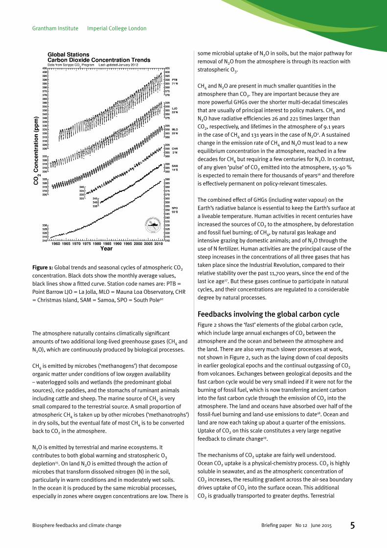
Carbon dioxide and other long-lived natural greenhouse gasesCarbon dioxide is essential to life. It is the basis of photosynthesis, and therefore all primary production, whether in natural ecosystems (marine or terrestrial) or on land used to produce food and other natural products such as timber, pulp, natural fabrics and biomass fuel. Time courses of CO2 in the atmosphere are shown in Figure 1, which shows the continuing increase, but also shows the effects of seasonal uptake and release of CO2 by terrestrial ecosystems. Terrestrial ecosystems are largely responsible for the seasonal cycle of CO2, due to the strong buffering effect of dissolved bicarbonate ions in seawater, which dampens the influence of seasonal variations in marine productivity on atmospheric CO2.



The atmosphere naturally contains climatically significant amounts of two additional long-lived greenhouse gases (CH4 and N2O), which are continuously produced by biological processes.

CH4 is emitted by microbes (‘methanogens’) that decompose organic matter under conditions of low oxygen availability – waterlogged soils and wetlands (the predominant global sources), rice paddies, and the stomachs of ruminant animals including cattle and sheep. The marine source of CH4 is very small compared to the terrestrial source. A small proportion of atmospheric CH4 is taken up by other microbes (‘methanotrophs’) in dry soils, but the eventual fate of most CH4 is to be converted back to CO2 in the atmosphere.

N2O is emitted by terrestrial and marine ecosystems. It contributes to both global warming and stratospheric O3 depletion15. On land N2O is emitted through the action of microbes that transform dissolved nitrogen (N) in the soil, particularly in warm conditions and in moderately wet soils. In the ocean it is produced by the same microbial processes, especially in zones where oxygen concentrations are low. There is

some microbial uptake of N2O in soils, but the major pathway for removal of N2O from the atmosphere is through its reaction with stratospheric O3.

CH4 and N2O are present in much smaller quantities in the atmosphere than CO2. They are important because they are more powerful GHGs over the shorter multi-decadal timescales that are usually of principal interest to policy makers. CH4 and N2O have radiative efficiencies 26 and 221 times larger than CO2, respectively, and lifetimes in the atmosphere of 9.1 years in the case of CH4 and 131 years in the case of N2O2. A sustained change in the emission rate of CH4 and N2O must lead to a new equilibrium concentration in the atmosphere, reached in a few decades for CH4 but requiring a few centuries for N2O. In contrast, of any given ‘pulse’ of CO2 emitted into the atmosphere, 15-40 % is expected to remain there for thousands of years16 and therefore is effectively permanent on policy-relevant timescales.

The combined effect of GHGs (including water vapour) on the Earth’s radiative balance is essential to keep the Earth’s surface at a liveable temperature. Human activities in recent centuries have increased the sources of CO2 to the atmosphere, by deforestation and fossil fuel burning; of CH4, by natural gas leakage and intensive grazing by domestic animals; and of N2O through the use of N fertilizer. Human activities are the principal cause of the steep increases in the concentrations of all three gases that has taken place since the Industrial Revolution, compared to their relative stability over the past 11,700 years, since the end of the last ice age17. But these gases continue to participate in natural cycles, and their concentrations are regulated to a considerable degree by natural processes.

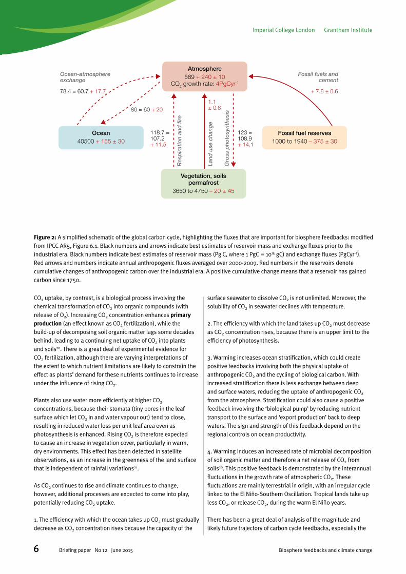
Feedbacks involving the global carbon cycleFigure 2 shows the ‘fast’ elements of the global carbon cycle, which include large annual exchanges of CO2 between the atmosphere and the ocean and between the atmosphere and the land. There are also very much slower processes at work, not shown in Figure 2, such as the laying down of coal deposits in earlier geological epochs and the continual outgassing of CO2 from volcanoes. Exchanges between geological deposits and the fast carbon cycle would be very small indeed if it were not for the burning of fossil fuel, which is now transferring ancient carbon into the fast carbon cycle through the emission of CO2 into the atmosphere. The land and oceans have absorbed over half of the fossil-fuel burning and land-use emissions to date18. Ocean and land are now each taking up about a quarter of the emissions. Uptake of CO2 on this scale constitutes a very large negative feedback to climate change19.

The mechanisms of CO2 uptake are fairly well understood. Ocean CO2 uptake is a physical-chemistry process. CO2 is highly soluble in seawater, and as the atmospheric concentration of CO2 increases, the resulting gradient across the air-sea boundary drives uptake of CO2 into the surface ocean. This additional CO2 is gradually transported to greater depths. Terrestrial

Figure 1: Global trends and seasonal cycles of atmospheric CO2 concentration. Black dots show the monthly average values, black lines show a fitted curve. Station code names are: PTB = Point Barrow LJO = La Jolla, MLO = Mauna Loa Observatory, CHR = Christmas Island, SAM = Samoa, SPO = South Pole92



CO2 uptake, by contrast, is a biological process involving the chemical transformation of CO2 into organic compounds (with release of O2). Increasing CO2 concentration enhances primary production (an effect known as CO2 fertilization), while the build-up of decomposing soil organic matter lags some decades behind, leading to a continuing net uptake of CO2 into plants and soils20. There is a great deal of experimental evidence for CO2 fertilization, although there are varying interpretations of the extent to which nutrient limitations are likely to constrain the effect as plants’ demand for these nutrients continues to increase under the influence of rising CO2.

Plants also use water more efficiently at higher CO2 concentrations, because their stomata (tiny pores in the leaf surface which let CO2 in and water vapour out) tend to close, resulting in reduced water loss per unit leaf area even as photosynthesis is enhanced. Rising CO2 is therefore expected to cause an increase in vegetation cover, particularly in warm, dry environments. This effect has been detected in satellite observations, as an increase in the greenness of the land surface that is independent of rainfall variations21.

As CO2 continues to rise and climate continues to change, however, additional processes are expected to come into play, potentially reducing CO2 uptake.

1. The efficiency with which the ocean takes up CO2 must gradually decrease as CO2 concentration rises because the capacity of the

surface seawater to dissolve CO2 is not unlimited. Moreover, the solubility of CO2 in seawater declines with temperature.

2. The efficiency with which the land takes up CO2 must decrease as CO2 concentration rises, because there is an upper limit to the efficiency of photosynthesis.

3. Warming increases ocean stratification, which could create positive feedbacks involving both the physical uptake of anthropogenic CO2 and the cycling of biological carbon. With increased stratification there is less exchange between deep and surface waters, reducing the uptake of anthropogenic CO2 from the atmosphere. Stratification could also cause a positive feedback involving the ‘biological pump’ by reducing nutrient transport to the surface and ‘export production’ back to deep waters. The sign and strength of this feedback depend on the regional controls on ocean productivity.

4. Warming induces an increased rate of microbial decomposition of soil organic matter and therefore a net release of CO2 from soils20. This positive feedback is demonstrated by the interannual fluctuations in the growth rate of atmospheric CO2. These fluctuations are mainly terrestrial in origin, with an irregular cycle linked to the El Niño-Southern Oscillation. Tropical lands take up less CO2, or release CO2, during the warm El Niño years.

There has been a great deal of analysis of the magnitude and likely future trajectory of carbon cycle feedbacks, especially the

Atmosphere589 + 240 ± 10

CO2 growth rate: 4PgCyr-1

Vegetation, soilspermafrost

3650 to 4750 – 20 ± 45

Ocean40500 + 155 ± 30

Fossil fuel reserves1000 to 1940 – 375 ± 30

Ocean-atmosphereexchange

Fossil fuels andcement

Res

pir

atio

n an

d fi

re

Land

use

cha

nge

Gro

ss p

hoto

synt

hesi

s

118.7 =107.2 + 11.5

123 =108.9 + 14.1

+ 7.8 ± 0.6

1.1 ± 0.8

78.4 = 60.7 + 17.7

80 = 60 + 20

Figure 2: A simplified schematic of the global carbon cycle, highlighting the fluxes that are important for biosphere feedbacks: modified from IPCC AR5, Figure 6.1. Black numbers and arrows indicate best estimates of reservoir mass and exchange fluxes prior to the industrial era. Black numbers indicate best estimates of reservoir mass (Pg C, where 1 PgC = 1015 gC) and exchange fluxes (PgCyr-1). Red arrows and numbers indicate annual anthropogenic fluxes averaged over 2000-2009. Red numbers in the reservoirs denote cumulative changes of anthropogenic carbon over the industrial era. A positive cumulative change means that a reservoir has gained carbon since 1750.



terrestrial carbon feedbacks: both the negative feedback due to CO2 fertilization, which is currently dominant, and the positive feedback due to increased microbial activity, which is expected to become progressively more important as temperatures rise.

Permafrost carbon feedback is a more recent concern. It has become clear that large, previously unaccounted quantities of carbon are stored in permanently frozen soils22,23. Between the LGM and the present interglacial there was a reduction in ‘inert’ carbon stored in permafrost24, due to thawing of part of the permafrost area. Further warming is expected to release additional CO2 from the remainder of this store. This is a positive feedback involving the carbon cycle, which was discussed (and quantitative estimates given) in AR5, but was not included in any of the Earth System Models participating in AR5. It is very difficult to quantify because of uncertainty about the rate and depth of thawing, and about the rate of carbon release when thawing occurs.

Feedbacks involving other long-lived greenhouse gasesAs with CO2, warming increases natural emission rates of CH4 from the biosphere – principally from waterlogged soils and wetlands, which are the largest sources of CH4

25. This implies a positive feedback. Warming also increases the rate of N2O emission from both natural and agricultural soils, leading to an increase in the atmospheric concentration of N2O, and thus another positive feedback26. The response of the ocean source of N2O is more complicated. Increased stratification tends to reduce marine productivity and therefore the rate of N cycling in the upper ocean. This would produce a negative feedback as the rate of emission of N2O would be reduced. On the other hand, warming is also expected to increase the extent of oxygen minimum zones in the ocean, which are a large source of N2O. This would produce a positive feedback. The net marine N2O feedback is therefore of unknown sign, but expected to be small.

For CH4 the story is complicated by a variable atmospheric lifetime. The lifetime of CH4 depends on the concentration of a short-lived but highly effective atmospheric oxidant, the hydroxyl radical (OH). OH is produced continuously in the atmosphere during the daytime through the action of ultraviolet radiation on O3 in the presence of water vapour. Warming increases the atmospheric water vapour content and therefore also the concentration of OH, an effect which tends to reduce the lifetime (and concentration) of CH4 – a negative feedback. In addition, the reaction between OH and CH4 proceeds more rapidly at higher temperatures – another negative feedback. On the other hand, as the concentration of CH4 increases, the limited oxidizing capacity (OH concentration) of the atmosphere can become more and more stretched, resulting in an increase in the lifetime (and concentration) of CH4 – a positive feedback.

In addition to CH4 in the atmosphere, vast stores (thought to exceed the total global amount of all conventional fossil fuels) of CH4 occur in continental shelf and slope sediments in the form of

hydrates (clathrates), in which CH4 molecules are trapped in an ice lattice. Methane hydrates are stable at the low temperatures (a few degrees above 0˚C) and high pressures encountered on the sea floor. A concern has been expressed that global warming could destabilize marine CH4 hydrates, leading in the worst case to a massive release of CH4 with catastrophic consequences for climate and the world economy27; or if the release were slower, to a large additional release of CO2 (the CH4 being oxidized to CO2 during passage from the sediments to the atmosphere). The qualitative conclusion that carbon will be released from marine CH4 hydrates, due to warming of bottom water, is supported by modelling. However, modelling has also shown that the sea bed cannot warm rapidly, and therefore the rate of release is expected to be extremely slow3 . Over centuries, the magnitude of this feedback could be comparable with the climate-CO2 feedback1. A future source of CH4 from permafrost thawing is also possible, although at present this is a tiny component of the global CH4 budget1. A small additional source of N2O from permafrost thawing is also possible, but unquantified.

The current state of the Earth is very different from the Palaeocene-Eocene Thermal Maximum, about 55 million years ago, when CH4 release from hydrates may have been the cause of a major global climate warming. This episode occurred on an ice-free Earth with deep ocean temperatures at least 10˚C warmer than today. Much more recently (8,200 years ago) the largest known marine landslide (the Storegga event), which has been putatively linked to CH4 hydrate destabilization28, did not result in any measurable change in the concentration of atmospheric CH4 as recorded in ice cores. Palaeodata from the Last Interglacial (about 130,000 to 120,000 years ago) provide a further constraint on this process. At this time annual solar radiation at high northern latitudes was unusually large, and mean annual land temperatures around the Arctic were 5-10˚C higher than present28-30. However, ice-core records of atmospheric CH4 over this interval do not show a ‘spike’ that would indicate a rapid release of CH4 from any source at any time during the Last Interglacial.

Biogeophysical feedbacksChanges in the distribution of vegetation in response to changes in temperatures and atmospheric CO2 can influence climate through physical effects, including the positive feedback due to the snow masking effect of forests in high latitudes. CO2 fertilization is primarily a mechanism generating net carbon uptake by the land; but as CO2 increases green vegetation cover (‘greening’) in water-stressed regions, as recently demonstrated21, it also generally reduces the albedo of the land surface and could therefore produce a positive feedback32. Reduced transpiration from leaves in response to rising CO2 might have consequences for the hydrological cycle (reduced evapotranspiration and increased runoff). However, this effect is opposed by ‘greening’ which increases the transpiring surface area33.

Why are biosphere feedbacks policy-relevant?Countries have expressed a political goal of keeping the global mean temperature rise below 2°C. As CO2 accumulates in



the atmosphere, to achieve this or any other global warming target, emissions of CO2 will need to be reduced over time and eventually phased out34. This qualitative conclusion is based on the fact that about 15 to 40% of any CO2 emissions will remain in the atmosphere for thousands of years until they are gradually removed from the atmosphere by extremely slow processes (carbonate dissolution in the ocean and silicate rock weathering on land), well beyond the time scales of policy relevance.

The magnitude and timing of the required reductions, however, depends on the future of the carbon cycle feedbacks, and also the feedbacks involving other GHGs (as these alter the degree of warming associated with a given concentration of CO2). The UK is committed to an 80% reduction in CO2 emissions by 205035. These recommendations were made on the basis of climate model calculations, which predict the changes in climate to be expected under different future scenarios, together with carbon cycle calculations that take into account the range of uncertainty among carbon cycle models concerning the magnitude of both the negative and the positive carbon cycle feedbacks.

It has been suggested that the level of warming to be expected in scenarios of future emissions might have been underestimated due to neglect of positive feedbacks36. Any additional positive feedback would mean that emissions targets need to be stiffer in order to achieve climate stabilisation at a given level. Some specific additional feedback processes are indeed both significant in magnitude and not included in current models, most notably the potential additional positive climate-CO2 feedback due to the decomposition of organic carbon stored in thawing permafrost.

We are considering here feedbacks that act on time scales up to about a century. We do not consider, for example, the positive feedback (due to increased absorption of solar radiation) likely to result from extensive or complete melting of the Greenland ice sheet. Such slow physical feedbacks are not included in climate models, nor in the definition of climate sensitivity37. Similarly, we do not analyse the processes that are expected to remove anthropogenic CO2 from the atmosphere over thousands to hundreds of thousands of years into the distant future. Our analysis refers to feedbacks that are expected to be effective on time scales consistent with the policy-relevant time frame (decades to centuries) adopted by the IPCC.

Quantitative understanding of century-scale feedbacks overall remains incomplete but the situation is improving, as documented here. Quantification is important because without it, the strength and expected future development of feedbacks will remain uncertain, leading to persistent uncertainties about the expected effects of any climate mitigation policy on the real climate.

Feedbacks in modelsGCMs include explicit representations of the fast physical feedbacks involving the Earth’s radiative balance, snow cover,

sea-ice cover, atmospheric water vapour and clouds. But they require GHG concentrations to be specified. The main set of future projections carried out with climate models for AR5 were performed using a series of scenarios called ‘representative concentration pathways’ (RCPs), which specify 21st century time-courses of the concentration of CO2 and other atmospheric constituents on a trajectory towards stabilization at a total radiative forcing of 2.6, 4.5 and 6.0 W m–2, plus a ‘business as usual’ scenario that reaches 8.5 W m–2 by the end of the century.

Climate models that also include a carbon cycle – that is, they predict the fate of CO2 emissions, including uptake by the land and oceans, and the effects of climate change on CO2 uptake and release by the land and ocean – have existed since the early 2000s. Results from these models were compared in the C4MIP project, and analysed in the IPCC Fourth Assessment Report (AR4)38. By the time of AR5, many climate modelling groups had continued to develop these coupled models further, including additional biogeochemical processes and feedbacks in many cases. These new-generation models are called Earth System models (ESMs). AR5 features model runs performed with a number of ESMs, alongside those done with standard GCMs. ESMs predict atmospheric CO2 concentration, given scenarios of emissions. They take into account the main ocean and land carbon cycle feedbacks (although not yet the permafrost carbon feedback). When used to project forward under the RCPs for AR5, the ESMs were prescribed year-by-year concentrations in the same way as for standard GCMs – but the ESMs could then infer what CO2 emissions would be consistent with each RCP.

Unfortunately, large differences among ESMs were found in both the C4MIP and AR4 analyses39-41. The models made widely ranging predictions about the strengths of the major feedbacks and how they evolve. The underlying problem is that the carbon cycle components of current ESMs are not well constrained with observations42. The C4MIP analysis already featured predictions of ‘extra’ CO2 in the atmosphere by 2100 (due to feedbacks) that differed by a factor of 7.5 between the smallest and the largest. The reasons for the differences were explored in the AR4. It was found that models differed greatly in the extent to which rising CO2 stimulated primary production on land; while not even the sign of the response of primary production to global warming was consistent among models. Similar comparisons of the more recent model runs in the AR5 showed no better agreement. Thus, feedback strengths cannot yet be estimated with satisfactory precision based on ESMs alone. On the other hand, as we will show, uncertainty caused by differences among models can be greatly reduced through the application of observational constraints.

Abrupt climate change and tipping pointsPalaeoclimate data show that the Earth system has experienced periods of exceptionally rapid changes between states, most recently at the beginning of the present interglacial (11,700 years ago). Earlier rapid changes include Dansgaard-Oeschger (D-O) events: repeated episodes of rapid, near-global warming followed



by gradual cooling, which punctuated the most recent and previous glacial periods43.

Rapid changes of state are symptomatic of tipping points. Tipping points can arise when feedbacks act to maintain a system in a fixed state until a threshold is crossed, at which point the system shifts to a substantially different state44. Such behaviour has not been seen in the Earth system during the past 8000 years, by which time the large continental ice sheets had dwindled to a small fraction of their size at the LGM. There is no specific reason to expect new global-scale tipping points to be crossed as a result of projected climate changes, and GCM and ESM simulations do not predict such occurrences for the 21st century. However, a number of potential regional tipping points, or tipping ‘elements’, have been identified as possible consequences of climate change, or the interaction of climate and land-use change, during coming centuries44. One example is the possible dieback of the Amazon rainforest, which was predicted by some early ESMs. With the exception of the permafrost carbon feedback, the mechanisms involved are represented in current ESMs – although we do not know how realistically.

Estimated magnitudes of feedbacks

Background to the technical reviewThe strength of feedbacks can vary according to scenario, model or method used to calculate them45,46

. This section presents our current assessment of the major biosphere-climate feedbacks. It draws on the work by Arneth et al.25 for terrestrial processes, and the more recent IPCC summary of feedbacks (Figure 6.20 in AR5)18, while updating these analyses with information from recently published work. We consider land and ocean carbon responses to CO2 concentration and temperature, and feedbacks involving permafrost carbon, biospheric emissions of CH4, the atmospheric lifetime of CH4, and biospheric emissions of N2O. These are the largest feedbacks involving atmospheric composition according to AR5. AR5 also lists a number of much smaller feedbacks – positive, negative, or of uncertain sign – which we do not attempt to quantify, but discuss briefly for completeness.

A common ‘currency’ is needed so that the magnitudes of different feedbacks can be compared. We adopt the dimensionless quantity used in control engineering known as the gain. This is a measure of the extent to which a feedback amplifies (if gain is positive) or diminishes (if gain is negative) the change in global mean temperature that would be expected in the absence of the feedback. If a feedback has a gain of 0.1, for example, this means that the change without the feedback would be 10% smaller than the change including the feedback. Gain has the attractive property that the gains due to several independent feedbacks can be added up (Box A). However, this does not mean that the resulting increments of temperature change can be added up. For example, as positive feedbacks

accumulate, the increments of temperature increase more steeply. In this review, for quantifying carbon cycle feedbacks, the radiative efficiency of CO2 was assigned a value of 0.0049 W m–2

Pg C–1, following Gregory et al.47. Thus we arrived at values for the feedback strength in W m –2 K–1. We then converted these to gain by multiplying by a climate sensitivity of 3˚C.

Table 1 shows calculations of gain, based on our assessment of the literature. Our calculations apply explicitly to the centennial time scale: that is, we calculated feedback strengths based on modelled concentrations at 2100 in simulations forced by changes in GHG emissions and climate starting in pre-industrial time. Table 1 includes calculations by Stocker et al.46, who modelled GHG and albedo feedbacks involving the land biosphere using the LPX-Bern 1.0 model under the ‘business as usual’ RCP 8.5 and ‘high mitigation’ RCP 2.6 scenarios. Estimates of the relevant gains under RCP 8.5 at 2100 are shown. Stocker et al. also considered the sensitivity of biosphere feedbacks to both time and scenario. For example, the negative feedback from CO2 fertilization decreases over time under the high-emissions scenario due to saturation of the photosynthetic response, combined with the declining radiative efficiency of CO2 at high concentrations. This study is unique so far in simultaneously quantifying feedbacks linked to CO2, CH4 and N2 O and surface albedo changes in a consistent way within a single model.

Land carbon cycle feedbacks General findings

Increased atmospheric CO2 is driving an increase in global primary production, which in turn is causing net CO2 uptake by the terrestrial biosphere. This is the CO2-concentration feedback, with a negative sign. But higher temperatures lead to a higher rates of microbial CO2 release from soils. This is the climate-CO2 feedback, with a positive sign. ESM estimates of both effects vary widely. In Table 1, values are given based on both the C4MIP and CMIP5 analyses. Both showed the negative CO2-concentration feedback to be larger than the positive climate-CO2 feedback throughout the 21st century. The C4MIP estimates were calculated at 2100 under the Special Report on Emissions Scenarios (SRES) A2 scenario25,48; the CMIP5 estimates were also calculated at 2100 but using a scenario where CO2 concentrations are increased at a rate of 1% per year45. The differences between the scenarios could be one underlying reason for the differences in modelled feedback strengths, as well as differences in the set of models participating, and changes to the models.

Following the method of Arneth et al., we converted land CO2-concentration feedback strengths to ‘gain’ using published values of the models’ ‘climate resistance’47,49, the inverse of climate sensitivity (Box A). Some models used in CMIP5 were excluded because their climate resistance values were not available.

Nutrient limitations

Nitrogen is required for primary production, and N supply is limiting to plant growth at least in most temperate and cold-

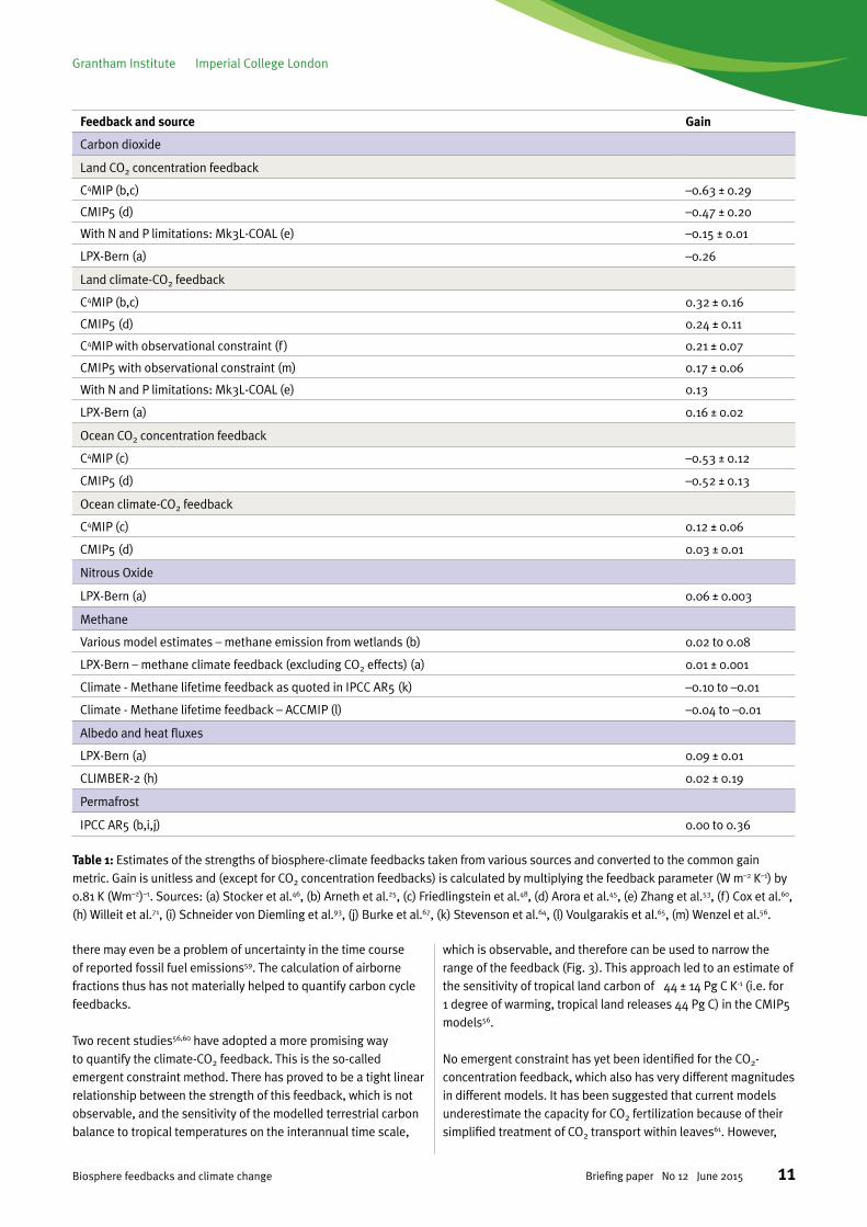
Table 1: Estimates of the strengths of biosphere-climate feedbacks taken from various sources and converted to the common gain metric. Gain is unitless and (except for CO2 concentration feedbacks) is calculated by multiplying the feedback parameter (W m–2 K–1) by 0.81 K (Wm–2)–1. Sources: (a) Stocker et al.46, (b) Arneth et al.25, (c) Friedlingstein et al.48, (d) Arora et al.45, (e) Zhang et al.53, (f) Cox et al.60, (h) Willeit et al.71, (i) Schneider von Diemling et al.93, (j) Burke et al.67, (k) Stevenson et al.64, (l) Voulgarakis et al.65, (m) Wenzel et al.56.



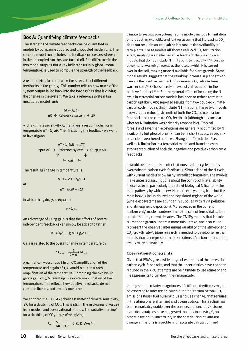
Box A: Quantifying climate feedbacksThe strengths of climate feedbacks can be quantified in models by comparing coupled and uncoupled model runs. The coupled model run includes the feedback processes whereas in the uncoupled run they are turned off. The difference in the two model outputs (for a key indicator, usually global mean temperature) is used to compute the strength of the feedback.

A useful metric for comparing the strengths of different feedbacks is the gain, g. This number tells us how much of the system output is fed back into the forcing (ΔR) that is driving the change in the system. We take a reference system (an uncoupled model run):

ΔT0= λ0 ΔRΔR → Reference system → ΔR

with a climate sensitivity λ0 that gives a resulting change in temperature ΔT = λ0 ΔR. Then including the feedback we want to investigate:

ΔT = λ0 (ΔR + c1ΔT)Input ΔR → Reference system → Output ΔR

↑ ↓← c1ΔT ←

The resulting change in temperature is

ΔT = λ0ΔR + λ0c1ΔTor

ΔT = λ0ΔR + gΔT

in which the gain, g, is equal to

g = λ0c1

An advantage of using gain is that the effects of several independent feedbacks can simply be added together:

ΔT = λ0ΔR + g1ΔT + g2ΔT + …

Gain is related to the overall change in temperature by

ΔTnew = ( 1 ) ΔTorig

A gain of 1/3 would result in a 50% amplification of the temperature and a gain of 1/2 would result in a 100% amplification of the temperature. Combining the two would give a gain of 5/6, resulting in a 600% amplification of the temperature. This reflects how positive feedbacks do not combine linearly, but amplify one other.

We adopted the IPCC AR4 ‘best estimate’ of climate sensitivity, 3˚C for a doubling of CO2. This is still in the mid-range of values from models and observational studies. The radiative forcing3 for a doubling of CO2 is 3.7 Wm-2, giving:

λ0 = ΔT = 3 = 0.81 K (Wm-2)-1.

climate terrestrial ecosystems. Some models include N limitation on production explicitly, and further assume that increasing CO2 does not result in an equivalent increase in the availability of N to plants. These models all show a reduced CO2 fertilization effect, implying a smaller negative feedback than is shown in models that do not include N limitations to growth24,50-52. On the other hand, warming increases the rate at which N is turned over in the soil, making more N available for plant growth. Some model results suggest that the resulting increase in plant growth cancels the positive feedback of increased CO2 release from warmer soils52. Others merely show a slight reduction in the positive feedback50,51. But the general effect of including the N cycle in terrestrial carbon models has been to reduce terrestrial carbon uptake25. AR5 reported results from two coupled climate-carbon cycle models that include N limitations. These two models show greatly reduced strength of both the CO2-concentration feedback and the climate-CO2 feedback (although it is unclear whether N limitation was primarily responsible). Tropical forests and savannah ecosystems are generally not limited by N availability but phosphorus (P) can be in short supply, especially on ancient weathered surfaces. Zhang et al.53 included P as well as N limitation in a terrestrial model and found an even stronger reduction of both the negative and positive carbon cycle feedbacks.

It would be premature to infer that most carbon cycle models overestimate carbon cycle feedbacks. Simulations of the N cycle with current models show many unrealistic features54. The models make untested assumptions about the control of N availability in ecosystems, particularly the rate of biological N fixation – the main pathway by which ‘new’ N enters ecosystems, in all but the most heavily industrialized and populated regions of the world (where ecosystems are abundantly supplied with N via pollution and atmospheric deposition). Moreover, even the current ‘carbon only’ models underestimate the rate of terrestrial carbon uptake55 during recent decades. The CMIP5 models that include N limitation greatly underestimate this uptake, and also fail to represent the observed interannual variability of the atmospheric CO2 growth rate56. More research is needed to develop terrestrial models that can represent the interactions of carbon and nutrient cycles more realistically.

Observational constraints

Given that ESMs give a wide range of estimates of the terrestrial carbon cycle feedbacks, and that the uncertainties have not been reduced in the AR5, attempts are being made to use atmospheric measurements to pin down their magnitude.

Changes in the relative magnitudes of different feedbacks might be expected to alter the so-called airborne fraction of total CO2 emissions (fossil fuel burning plus land-use change) that remains in the atmosphere after land and ocean uptake. This fraction has been remarkably stable over the past several decades57. Some statistical analyses have suggested that it is increasing58, but others have not57. Uncertainty in the contribution of land-use change emissions is a problem for accurate calculation, and



there may even be a problem of uncertainty in the time course of reported fossil fuel emissions59. The calculation of airborne fractions thus has not materially helped to quantify carbon cycle feedbacks.

Two recent studies56,60 have adopted a more promising way to quantify the climate-CO2 feedback. This is the so-called emergent constraint method. There has proved to be a tight linear relationship between the strength of this feedback, which is not observable, and the sensitivity of the modelled terrestrial carbon balance to tropical temperatures on the interannual time scale,

which is observable, and therefore can be used to narrow the range of the feedback (Fig. 3). This approach led to an estimate of the sensitivity of tropical land carbon of −44 ± 14 Pg C K-1 (i.e. for 1 degree of warming, tropical land releases 44 Pg C) in the CMIP5 models56.

No emergent constraint has yet been identified for the CO2-concentration feedback, which also has very different magnitudes in different models. It has been suggested that current models underestimate the capacity for CO2 fertilization because of their simplified treatment of CO2 transport within leaves61. However,

Feedback and source Gain

Carbon dioxide

Land CO2 concentration feedback

C4MIP (b,c) –0.63 ± 0.29

CMIP5 (d) –0.47 ± 0.20

With N and P limitations: Mk3L-COAL (e) –0.15 ± 0.01

LPX-Bern (a) –0.26

Land climate-CO2 feedback

C4MIP (b,c) 0.32 ± 0.16

CMIP5 (d) 0.24 ± 0.11

C4MIP with observational constraint (f ) 0.21 ± 0.07

CMIP5 with observational constraint (m) 0.17 ± 0.06

With N and P limitations: Mk3L-COAL (e) 0.13

LPX-Bern (a) 0.16 ± 0.02

Ocean CO2 concentration feedback

C4MIP (c) –0.53 ± 0.12

CMIP5 (d) –0.52 ± 0.13

Ocean climate-CO2 feedback

C4MIP (c) 0.12 ± 0.06

CMIP5 (d) 0.03 ± 0.01

Nitrous Oxide

LPX-Bern (a) 0.06 ± 0.003

Methane

Various model estimates – methane emission from wetlands (b) 0.02 to 0.08

LPX-Bern – methane climate feedback (excluding CO2 effects) (a) 0.01 ± 0.001

Climate - Methane lifetime feedback as quoted in IPCC AR5 (k) –0.10 to –0.01

Climate - Methane lifetime feedback – ACCMIP (l) –0.04 to –0.01

Albedo and heat fluxes

LPX-Bern (a) 0.09 ± 0.01

CLIMBER-2 (h) 0.02 ± 0.19

Permafrost

IPCC AR5 (b,i,j) 0.00 to 0.36

Table 1: Estimates of the strengths of biosphere-climate feedbacks taken from various sources and converted to the common gain metric. Gain is unitless and (except for CO2 concentration feedbacks) is calculated by multiplying the feedback parameter (W m–2 K–1) by 0.81 K (Wm–2)–1. Sources: (a) Stocker et al.46, (b) Arneth et al.25, (c) Friedlingstein et al.48, (d) Arora et al.45, (e) Zhang et al.53, (f ) Cox et al.60, (h) Willeit et al.71, (i) Schneider von Diemling et al.93, (j) Burke et al.67, (k) Stevenson et al.64, (l) Voulgarakis et al.65, (m) Wenzel et al.56.



this is only one of many potential issues with the way CO2 effects on plants are represented in models.

Ocean carbon cycle feedbacksNet CO2 uptake by the ocean is driven by rising CO2 concentration, which causes a difference in the partial pressure of CO2 across the air-sea boundary which, in turn, drives CO2 uptake. Warming however leads to increased stratification, leading in turn to reduced CO2 uptake. This positive feedback appears to be small. There is an interaction between the effect of warming and the effect of reduced CO2 uptake at high CO2 concentration62. Nonetheless, both C4MIP and CMIP5 estimates of the negative feedback due to ocean uptake are much larger than estimates of the positive feedback due to warming (Table 1).

Nitrous oxide feedbacksThe terrestrial emission of N2O is mainly due to denitrification, a microbial process by which dissolved nitrate in the soil is transformed into the gases NO, N2O and N2

46. The rate of denitrification is strongly temperature-dependent, with an optimum as high as 38°C26. Warming also tends to increase the availability of N for microbial action46. Terrestrial N2O emissions are therefore expected to be enhanced in a warmer climate, resulting in a positive climate feedback. In Table 1, we cite Stocker et al.’s46 estimate from LPX-Bern, whose N cycle representation is based on that of Xu-Ri et al.26. Stocker et al.’s estimate applies to the centennial time scale and is thus comparable to estimates of carbon cycle feedbacks in Table 1. However, this calculation excludes agricultural land. Inclusion of emissions from fertilized agricultural land would increase the gain.

There is no available quantitative estimate of the net ocean N2O feedback, and even the terrestrial N2O feedback has not been directly constrained by observations. Potentially, information from past, natural changes in N2O concentration as shown in ice-core records63 could potentially help to constrain the magnitude of the total N2O feedback.

Methane feedbacksMethane lifetime

Although not strictly a biosphere feedback, we consider the ‘methane lifetime feedback’ here because CH4 is predominantly of biological origin, as are other atmospheric constituents that can influence the lifetime (and therefore the concentration) of CH4 in the atmosphere. Conflicting chemical impacts on methane lifetime arise as a result of different atmospheric concentrations of CH4, CO, O3 and OH. The negative feedback on methane lifetime quoted in AR5 is based on model results in Stevenson et al.64 – who found that higher temperatures led to an increase in the rate of methane oxidation with OH, and the corresponding higher humidity levels under a warmer climate led to a higher abundance of OH. In the Atmospheric Chemistry and Climate Modeling Intercomparison Project (ACCMIP), Voulgarakis et al.65 also found a negative feedback between climate and methane lifetime but noted that warmer climates enhance

stratosphere-troposphere exchange, leading to more O3 and OH in the troposphere, hence a shorter CH4 lifetime. Feedback strengths from both studies are included in Table 1. The strength of this feedback in most of the ACCMIP models is weaker than in earlier models that did not allow effects of temperature on O3 in the stratosphere to alter the rate of OH production in the troposphere.

Despite Voulgarakis et al.’s65 confirmation that increases in temperature should lead to a decrease in CH4 lifetime, under the future scenario RCP 8.5 they found the lifetime of CH4 actually increased (a positive climate feedback). This was due to the suppressive effect of a very large CH4 concentration on the concentration of OH.

Methane from wetlands

Under higher temperatures and higher atmospheric carbon dioxide concentrations, it is expected that natural CH4 emissions from wetlands will increase. Table 1 includes an estimate of this effect included in AR525, and the estimate by Stocker et al.46 The feedback strength due to methane emission from wetlands as estimated by Stocker et al. falls below the range of previous estimates by Arneth et al. Stocker et al. also found that changes in the concentration of CO2 were also an important driver of CH4 emissions, as did the multi-model study of wetlands and wetland CH4 emissions by Melton et al.66. The Stocker et al. estimate in Table 1 is for the effect of climate change alone.

Permafrost carbon feedbackThis is, on the basis of current knowledge, potentially the most important positive feedback on policy-relevant time scales that is currently not included in Earth System models67. The omission of permafrost carbon feedback from models is a concern for scientists working in the field as well as for policy makers68. A variety of ad hoc methods combining data and model results25, 67, 69 have produced a large range of estimates of the potential magnitude of this feedback. The range of values given in Table 1 was derived directly from the range given in AR5, and therefore is not discussed further here.

Biogeophysical feedbacksModels including vegetation responses to climate change in AR5 showed that in northern high latitudes, warming-induced vegetation expansion reduces surface albedo, enhancing warming over these regions. Over tropical forest, reduction of forest coverage reduces evapotranspiration, also leading to a regional warming69,70. In sensitivity studies with CLIMBER-2 (a simplified ESM), Willeit et al.71 showed that the sign of the total biogeophysical feedback is asymmetric: negative for a case where the CO2 concentration is doubled, and positive for a case where it is halved. We include the doubling CO2 feedback strength from their results here, as it is closer to the methods used to obtain the other feedback strengths, as well as being more relevant to future scenarios.



The biogeophysical feedback from the LPX-Bern falls within the range estimated using the CLIMBER-2 model71. However, the LPX-Bern ‘albedo’ feedback incorporates physical snow-ice albedo changes and vegetation albedo changes, whereas Willeit et al.33 considered changes solely due to vegetation. This accounts for the difference between the two estimates given in Table 1. Standard GCMs already include the physical feedback due to reduced snow and sea-ice cover, but they do not include the biogeophysical feedback due to vegetation changes.

Other biosphere feedbacksIPCC AR5 mentions other feedbacks involving the biosphere (e.g. the effects of biogenic emissions which have received some press coverage recently72), not included in Table 1 because (a) they are all very poorly quantified and (b) according to current understanding, their magnitude is small. They are listed here in summary form:

• Increasing emissions of biogenic volatile organic compounds (BVOCs) from plants. These compounds are involved in the generation of O3 in the atmosphere (depending on the background concentration of NOx

73) and their emission increases with the temperature of leaves74. Increasing BVOC emissions would tend to increase the production of secondary organic aerosols (SOA), which have a net cooling effect. The production of SOA is not well quantified. On the other hand, increasing CO2 tends to suppress BVOC emission75, an effect not considered in most models.

• Many other chemical mechanisms may influence atmospheric O3 concentration. O3 in the troposphere also has toxic effects on plants. Model calculations have suggested that effects of anthropogenically enhanced concentrations of O3 in populated areas may be significantly reducing terrestrial primary production76, and that O3 thus acts as an indirect greenhouse gas by reducing the strength of terrestrial CO2 uptake77.

• Changes in atmospheric dust concentration. The radiative effect of dust can be positive or negative depending on the underlying surface, time of day, dust properties and atmospheric state (e.g. water vapour, clouds)78. Dust can also affect climate through indirect interactions with clouds79 and alteration of biogeochemical cycles80. Dust emission could increase in some areas and decline in others, depending on changes in precipitation, vegetation cover and winds.

• Changes in marine dimethyl sulfide (DMS) emissions. DMS is a precursor of cloud condensation nuclei, with a net cooling effect that could act as a negative feedback in the climate system81. Increased ocean stratification however could reduce DMS emission.

• Fire has multiple climatic consequences, therefore a climatically induced change in fire regime would create feedbacks. Biomass burning releases carbon to the atmosphere more rapidly than it would be released by decomposition, so the total carbon storage on land is less (and the amount of CO2 in the atmosphere is greater) than

it would be in the absence of fire. Any increase in fire would further reduce terrestrial carbon storage and thereby add CO2 to the atmosphere. Both CH4 and N2O are also emitted in small quantities after fires. CO is emitted, which competes with CH4 for OH and therefore increases the lifetime of CH4, and also increases tropospheric O3. Black carbon (soot) is emitted. Black carbon is an absorbing aerosol with a net warming effect, compounded by its effect of reducing albedo when it falls on snow. These effects all promote warming. On the other hand, the emission of other organic compounds has been modelled to lead to a cooling due to the indirect aerosol effect that could be larger than all of the other effects combined82. Increased fire is often postulated as a consequence of warming83, possibly enhanced by CO2 (increased primary production leading to increased fuel loads)84, but countervailing effects have also been proposed85,86. The direction of the likely trend in biomass burning is thus uncertain, and even the sign of the fire feedback to climate is uncertain.

Policy implications

Mitigation scenarios and policyBiosphere feedbacks influence the relationship between emissions (of CO2 and other GHGs) and concentrations, which are what determine the greenhouse effect and thus the effect of emissions on climate. Biosphere feedbacks are therefore directly relevant for mitigation policy. Uncertainty about the magnitude of feedbacks is a problem for climate policy because the usefulness of climate projections is limited if the quantitative relationship between emissions and concentrations is unclear. Potentially large positive feedbacks are of particular concern, as positive feedbacks mean that more stringent emissions reductions are required to stabilize climate at any specified level. Moreover, multiple positive feedbacks are mutually reinforcing because of the non-linear relationship between temperature increase and gain. We have attempted to quantify the various feedbacks that have been proposed to be large – thus, those of greatest policy relevance.

A number of studies have related emissions to concentrations with the goal of specifying possible emissions ‘pathways’ consistent with stabilization of radiative forcing at different levels. Generally, these studies have realistically taken into account the most important feedbacks involving the carbon cycle, including the uncertainty arising from differences among ESMs. We have highlighted recent studies in which observations have been used to constrain the magnitude of terrestrial carbon cycle feedbacks, which continue to be represented very differently in models. The results of these studies indicate that earlier estimates of a large positive climate-CO2 feedback were excessive. The one key positive feedback (of still very uncertain magnitude) that has been omitted both from ESMs (as represented in AR5) and most assessments of emissions pathways is the release of CO2 into the atmosphere from thawing permafrost. However, this process was considered in AR5, is being included in next-generation ESMs, and was explicitly taken into account in the UK’s Fourth



Carbon Budget87 (Box B) along with carbon cycle feedbacks and feedbacks involving the CH4 lifetime and CH4 emissions from wetlands.

The ‘bottom line’ for mitigation policy is that the fraction of CO2 emissions that remains in the atmosphere after land and ocean uptake is, for all practical purposes, an irreversible addition to the radiative forcing of climate. Despite many residual uncertainties about feedbacks that are set in train by CO2 emissions, the fact remains that the expected global warming is approximately proportional to the total amount of CO2 that has been emitted (by fossil fuel burning, cement production and deforestation) since the Industrial Revolution88. This applies across all scenarios and models, and is perhaps the most striking result to have emerged from the AR5.

Human modification of biosphere feedbacksIn many respects biosphere feedbacks are an inescapable part of the climate system, acting on too large a scale to be substantially modified by deliberate interventions. However, there are certain ways in which human actions influence the magnitude of the feedbacks and therefore might provide additional scope for the mitigation of climate change.

• Avoid deforestation and forest degradation. This is the best known opportunity to maintain or enhance the CO2 concentration feedback, and it is being actively pursued in international climate negotiations. Carbon uptake by the biosphere is largely driven by forests, to a lesser extent by savannahs and grazing lands, and for practical purposes not at all by arable lands. Whilst recognizing that the principal reason for avoiding deforestation is to avoid releasing the carbon stocks they contain89, from a feedbacks perspective there is an additional incentive, i.e. to avoid reducing the capacity of the land to take up CO2 while CO2 concentrations continue to rise.

• Limit over-use of N fertilizers. The over-use of N fertilizer is a direct driver of anthropogenic N2 O emission (in particular, nitrogen that is not taken up by plants is liable to end up rapidly back in the atmosphere, some of it as N2O). The N2O feedback has been given relatively little consideration in the literature or in mitigation policy so far, perhaps because the full impact of increased emission on concentration of N2O will not be realized for several centuries. More careful targeting of N fertilizer use would reduce N2O emissions per unit area of land, or per unit of harvest. From a feedbacks perspective, reduced N fertilizer use would also limit the additional N2O emission expected (whether on natural or agricultural soils) in a warmer climate.

Physical land-surface changes associated with changing land use bring complexities that might help or hinder climate mitigation efforts. For example, forest clearance for expanded agriculture in high latitudes in some scenarios is calculated to have a regional cooling effect, offsetting the warming due to the release of the forest carbon stocks90.

Research agenda

Much of what we have summarized here relies on modelling. Models are an essential part of the toolkit of both atmospheric and ecosystem scientists, and ‘experiments’ with global models of ecosystem processes offer a natural way to estimate the strengths of different biosphere feedbacks. However the persistence of large differences in feedback estimates among ESMs, and the lack of demonstrable reductions in the range of modelled effects between successive IPCC reports, are sobering. More effort is needed to constrain models, using the observations that are available on the state and changes over recent decades of both the atmosphere and the biosphere. There is a notable lack of ‘joined-up’ thinking in the development of models that purport to represent understanding of ecosystem processes and yet fail to accurately represent the consequences for the atmosphere and thus for climate. A priority for research is for model development to become an integral part of ecosystem science, and for modelling centres to interact more closely with ecosystem scientists. This process goes well beyond model ‘benchmarking’, although the latter is essential and needs to be practised routinely42.

The emergent constraints methodology60 provides a potentially powerful route to use observations and models together to increase quantitative understanding of biosphere feedbacks, and could be applied to a wider range of feedbacks. Relevant observations are not confined to the recent period of intensive Earth observation. Palaeo evidence, from ice cores and terrestrial and marine sediments, is crucial in providing information on past states of the Earth that differed substantially from the present state. A top-priority target for research is the permafrost carbon feedback, which is likely to have been significantly involved in the regulation of atmospheric CO2 during the past million years.

We have accepted estimates in the current literature of which feedbacks are large and which are small. But many of those deemed to be small are not well quantified, and could contain surprises. Scientific areas where understanding is currently weak include the coupling of carbon and N cycles in terrestrial ecosystems and, more generally, the nature of feedbacks involving the terrestrial and marine N cycles; scenarios of future fire, and the sign and magnitude of feedbacks involving fire; the large-scale controls of BVOC emission and their implications for tropospheric O3 and the generation and climatic effects of SOA; the importance of cloud feedbacks involving DMS; and the role of dust in the climate system, anthropogenic versus natural contributions to atmospheric dust levels and the radiative forcing due to dust.

Acknowledgments

We thank Simon Buckle, Heather Graven and Apostolos Voulgarakis (Grantham Institute, Imperial College London), Jo House (Cabot Institute, University of Bristol), Philippe Ciais (Laboratoire des Sciences du Climat et de l’Environnement), and Chris Jones (Met Office) for their detailed and helpful reviews.



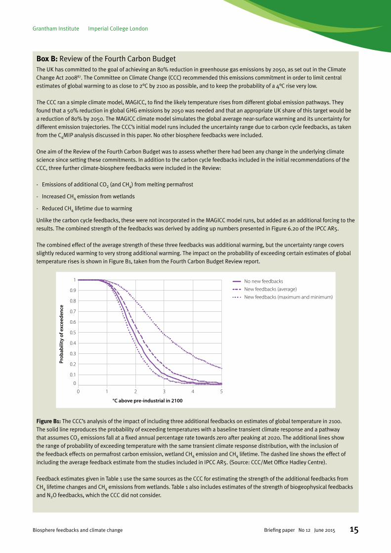
Box B: Review of the Fourth Carbon BudgetThe UK has committed to the goal of achieving an 80% reduction in greenhouse gas emissions by 2050, as set out in the Climate Change Act 200887. The Committee on Climate Change (CCC) recommended this emissions commitment in order to limit central estimates of global warming to as close to 2°C by 2100 as possible, and to keep the probability of a 4°C rise very low.

The CCC ran a simple climate model, MAGICC, to find the likely temperature rises from different global emission pathways. They found that a 50% reduction in global GHG emissions by 2050 was needed and that an appropriate UK share of this target would be a reduction of 80% by 2050. The MAGICC climate model simulates the global average near-surface warming and its uncertainty for different emission trajectories. The CCC’s initial model runs included the uncertainty range due to carbon cycle feedbacks, as taken from the C4MIP analysis discussed in this paper. No other biosphere feedbacks were included.

One aim of the Review of the Fourth Carbon Budget was to assess whether there had been any change in the underlying climate science since setting these commitments. In addition to the carbon cycle feedbacks included in the initial recommendations of the CCC, three further climate-biosphere feedbacks were included in the Review:

- Emissions of additional CO2 (and CH4) from melting permafrost

- Increased CH4 emission from wetlands

- Reduced CH4 lifetime due to warming

Unlike the carbon cycle feedbacks, these were not incorporated in the MAGICC model runs, but added as an additional forcing to the results. The combined strength of the feedbacks was derived by adding up numbers presented in Figure 6.20 of the IPCC AR5.

The combined effect of the average strength of these three feedbacks was additional warming, but the uncertainty range covers slightly reduced warming to very strong additional warming. The impact on the probability of exceeding certain estimates of global temperature rises is shown in Figure B1, taken from the Fourth Carbon Budget Review report.

Figure B1: The CCC’s analysis of the impact of including three additional feedbacks on estimates of global temperature in 2100. The solid line reproduces the probability of exceeding temperatures with a baseline transient climate response and a pathway that assumes CO2 emissions fall at a fixed annual percentage rate towards zero after peaking at 2020. The additional lines show the range of probability of exceeding temperature with the same transient climate response distribution, with the inclusion of the feedback effects on permafrost carbon emission, wetland CH4 emission and CH4 lifetime. The dashed line shows the effect of including the average feedback estimate from the studies included in IPCC AR5. (Source: CCC/Met Office Hadley Centre).

Feedback estimates given in Table 1 use the same sources as the CCC for estimating the strength of the additional feedbacks from CH4 lifetime changes and CH4 emissions from wetlands. Table 1 also includes estimates of the strength of biogeophysical feedbacks and N2O feedbacks, which the CCC did not consider.

Prob

abili

ty o

f exc

eede

nce

43210 5

0

0.1

0.2

0.3

0.4

0.5

0.6

0.7

0.8

0.9

1

°C above pre-industrial in 2100

No new feedbacks

New feedbacks (average)

New feedbacks (maximum and minimum)



We particularly thank Chris Jones for input on the CH4-lifetime feedback, Parvadha Suntharalingam (University of East Anglia) for authoritative information about the marine N2O feedback and Beni Stocker (Imperial College London) for providing feedback strength estimates from the LPX-Bern model. Natalie Crawley (Imperial College London) helped in finding literature and compiling the reference list. The paper benefited greatly from work by participants in the GREENCYCLES II Initial Training Network91, and especially from work presented at the GREENCYCLES II ‘Feedbacks Synthesis’ workshop led by ICP and held in Bristol in September 2013. This work is a contribution to the AXA Chair Programme on Biosphere and Climate Impacts, and the Imperial initiative on Grand Challenges in Ecosystems and the Environment.

References1. Martínez-Botí MA, Foster GL, Chalk TB et al. (2015) Plio-

Pleistocene climate sensitivity evaluated using high-resolution CO2 records. Nature 518: 49–54.

2. Myhre G, Shindell D, Bréon F et al. (2013) Anthropogenic and natural radiative forcing. In: Stocker TF, Qin D, Plattner G-K, et al., editors. Climate Change 2013: The Physical Science Basis. Contribution of Working Group I to the Fifth Assessment Report of the Intergovernmental Panel on Climate Change, Cambridge University Press, Cambridge

3. Collins M, Knutti R, Arblaster J et al. (2013) Long-term climate change: projections, commitments and irreversibility. In: Stocker TF, Qin D, Plattner G-K, et al., editors. Climate Change 2013: The Physical Science Basis. Contribution of Working Group 1 to the Fifth Assessment Report of the Intergovernmental Panel on Climate Change. Cambridge University Press. Cambridge.

4. Roe G. (2009) Feedbacks, timescales, and seeing red. Annual Review of Earth and Planetary Sciences 37: 93–115.

5. Forster P, Ramaswamy V, Artaxo P et al. (2007) Changes in atmospheric constituents and in radiative forcing. In: Solomon S, Qin D, Manning M, et al., editors. Climate Change 2007: The Physical Science Basis. Contribution of Working Group I to the Fourth Assessment Report of the Intergovernmental Panel on Climate Change. Cambridge University Press, Cambridge.

6. Boucher O, Randall D, Artaxo P, et al. (2013) Clouds and aerosols. In: Stocker TF, Qin D, Plattner G-K et al., editors. Climate Change 2013: The Physical Science Basis. Contribution of Working Group 1 to the Fifth Assessment Report of the Intergovernmental Panel on Climate Change. Cambridge University Press, Cambridge.

7. Flanner MG, Shell KM, Barlage M et al. (2011) Radiative forcing and albedo feedback from the Northern Hemisphere cryosphere between 1979 and 2008. Nature Geoscience 4: 151–155.

8. Otto A, Otto FEL, Boucher O et al. (2013) Energy budget constraints on climate response. Nature Geoscience 6: 415–416.

9. Sherwood SC, Bony S and Dufresne J-L (2014) Spread in model climate sensitivity traced to atmospheric convective mixing. Nature 505: 37–42.

10. Shindell DT (2014) Inhomogeneous forcing and transient climate sensitivity. Nature Climate Change 4: 274–277.

11. Schmittner A, Urban NM, Shakun JD et al. (2011) Climate sensitivity estimated from temperature reconstructions of the Last Glacial Maximum. Science 334: 1385–1388.

12. Hargreaves JC, Annan JD, Yoshimori M and Abe-Ouchi A (2012) Can the Last Glacial Maximum constrain climate sensitivity? Geophysical Research Letters 39, L24702.

13. Mactavish F, Buckle S (2013) Climate sensitivity. Grantham Briefing Note 2.

14. Hansen J, Sato M, Russell G and Kharecha, P (2013) Climate sensitivity, sea level and atmospheric carbon dioxide. Philosophical Transactions of the Royal Society A 371, 20120294.

15. Wuebbles DJ (2009) Nitrous oxide: no laughing matter. Science 326: 56–57.

16. Archer D, Eby M, Brovkin V et al. (2009) Atmospheric lifetime of fossil fuel carbon dioxide. Annual Review of Earth and Planetary Sciences 37: 117–134.

17. Hartmann D, Klein Tank A, Rusticucci M et al. (2013) Observations: atmosphere and surface. In: Stocker T, Qin D, Plattner G-K et al., editors. Climate Change 2013: The Physical Science Basis. Contribution of Working Group 1 to the Fifth Assessment Report of the Intergovernmental Panel on Climate Change. Cambridge University Press, Cambridge.

18. Ciais P, Sabine C, Bala G et al. Carbon and other biogeochemical cycles (2013) In: Stocker T, Qin D, Plattner G-K et al., editors. Climate Change 2013: The Physical Science Basis. Contribution of Working Group 1 to the Fifth Assessment Report of the Intergovernmental Panel on Climate Change. Cambridge University Press, Cambridge.

19. Shevliakova E, Pacala SW, Malyshev S et al. (2009) Carbon cycling under 300 years of land use change: Importance of the secondary vegetation sink. Global Biogeochemical Cycles 23, GB2022.

20. Heimann M and Reichstein M (2008) Terrestrial ecosystem carbon dynamics and climate feedbacks. Nature 451: 289–292.

21. Donohue RJ, Roderick ML, McVicar TR et al. (2013) Impact of CO2 fertilization on maximum foliage cover across the globe’s warm, arid environments. Geophysical Research Letters 40: 3031–3035.

22. Tarnocai C, Canadell JG, Schuur EAG et al. (2013) Soil organic carbon pools in the northern circumpolar permafrost region. Global Biogeochemical Cycles 23, GB2023.

23. Schuur EA, Vogel JG, Crummer KG et al. (2009) The effect of permafrost thaw on old carbon release and net carbon exchange from tundra. Nature 459: 556–559.

24. Ciais P, Tagliabue A, Cuntz M et al. (2011) Large inert carbon pool in the terrestrial biosphere during the Last Glacial Maximum. Nature Geoscience 5: 74–79.

25. Arneth A, Harrison SP, Zaehle S et al. (2010) Terrestrial biogeochemical feedbacks in the climate system. Nature Geoscience 3: 525–532.

26. Xu-Ri, Prentice IC, Spahni R and Niu HS (2012) Modelling terrestrial nitrous oxide emissions and implications for climate feedback. New Phytologist 196: 472–488.

27. Whiteman G, Hope C and Wadhams P (2013) Vast costs of Arctic change. Nature 499: 401–403.

28. Archer D (2007) Methane hydrate stability and anthropogenic climate change. Biogeosciences 4:521–544.



29. Turney CSM and Jones RT (2010) Does the Agulhas Current amplify global temperatures during super-interglacials? Journal of Quaternary Science 25: 839–843.

30. Velichko AA, Borisova OK and Zelikson EM (2008) Paradoxes of the Last Interglacial climate: reconstruction of the northern Eurasia climate based on palaeofloristic data. Boreas 37: 1–19.

31. Kienast F, Tarasov P, Schirrmeister L et al. (2008) Continental climate in the East Siberian Arctic during the last interglacial: Implications from palaeobotanical records. Global and Planetary Change 60: 535–562.

32. O’ishi R, Abe-Ouchi A, Prentice IC and Sitch S (2009) Vegetation dynamics and plant CO2 responses as positive feedbacks in a greenhouse world. Geophysical Research Letters 36, L11706.

33. Bala G, Caldeira K, Mirin A et al. (2006) Biogeophysical effects of CO2 fertilization on global climate. Tellus B 58: 620–627.

34. Solomon S, Plattner G, Knutti R et al. (2009) Irreversible climate change due to carbon dioxide emissions. Proceedings of the National Academy of Sciences of the United States of America 106: 1704–1709.

35. Anon. (2008) Climate Change Act 2008, Chapter 27. The Stationery Office, London.

36. Torn MS and Harte J (2006) Missing feedbacks, asymmetric uncertainties, and the underestimation of future warming. Geophysical Research Letters 33, L10703.

37. Previdi M, Liepert BG, Peteet D et al. (2013) Climate sensitivity in the Anthropocene. Quarterly Journal of the Royal Meteorological Society 139(A): 1121–1131.

38. Denman K, Brasseur G, Chidthaisong A et al. Couplings between changes in the climate system and biogeochemistry. In: Solomon S, Zin D, Manning M et al., editors. Climate Change 2007: The Physical Science Basis. Contribution of Working Group I to the Fourth Assessment Report of the Intergovernmental Panel on Climage Change. Cambridge University Press, Cambridge.

39. Anav A, Friedlingstein P, Kidston M et al. (2013) Evaluating the land and ocean components of the global carbon cycle in the CMIP5 Earth System Models. Journal of Climate 26: 6801–6843.

40. Friedlingstein P, Meinshausen M, Arora VK et al. (2014) Uncertainties in CMIP5 climate projections due to carbon cycle feedbacks. Journal of Climate 27: 511–526.

41. Friedlingstein P, Cox P, Betts R et al. (2006) Climate-carbon cycle feedback analysis: results from the C4MIP model intercomparison. Journal of Climate 19: 3337–3353.

42. Prentice IC, Liang X, Medlyn BE and Wang Y-P (2014) Reliable, robust and realistic: the three R’s of next-generation land surface modelling. Atmospheric Chemistry and Physics Discussions 14: 24811–24861.

43. Harrison SP and Sanchez-Goñi MF (2010) Global patterns of vegetation response to millennial-scale variability and rapid climate change during the last glacial period. Quaternary Science Reviews 29: 2957–2980.

44. Lenton T, Held H, Kriegler E et al. (2008) Tipping elements in the Earth’s climate system. Proceedings of the National Academy of Sciences of the United States of America 105: 1786–1793.

45. Arora VK, Boer GJ, Friedlingstein P et al. (2013) Carbon–concentration and carbon–climate feedbacks in CMIP5 Earth System Models. Journal of Climate 26: 5289–5314.

46. Stocker BD, Roth R, Joos F et al. (2013) Multiple greenhouse-gas feedbacks from the land biosphere under future climate change scenarios. Nature Climate Change 3 :666–672.

47. Gregory JM, Jones CD, Cadule P et al. (2009) Quantifying carbon cycle feedbacks. Journal of Climate 22 :5232–5250.

48. Friedlingstein P, Cox P, Betts R et al. (2006) Climate–carbon cycle feedback analysis: Results from the C4MIP model intercomparison. Journal of Climate 19: 3337–3353.

49. Forster PM, Andrews T, Good P et al. (2013) Evaluating adjusted forcing and model spread for historical and future scenarios in the CMIP5 generation of climate models. Journal of Geophysical Research 118: 1139–1150.

50. Sokolov AP, Kicklighter DW, Melillo JM et al. (2008) Consequences of considering carbon–nitrogen Interactions on the feedbacks between cimate and the terrestrial carbon cycle. Journal of Climate 21: 3776–3796.

51. Thornton P, Doney S, Lindsay K et al. (2009) Carbon-nitrogen interactions regulate climate-carbon cycle feedbacks: results from an atmosphere-ocean eneral circulation model. Biogeosciences 6: 2099–2120.

52. Zaehle S, Friedlingstein P and Friend AD (2010) Terrestrial nitrogen feedbacks may accelerate future climate change. Geophysical Research Letter 37, L01401.

53. Zhang Q, Wang Y, Matear RJ et al. (2014) Nitrogen and phosphorus limitations significantly reduce future allowable CO2 emissions. Geophysical Research Letters 41: 632–637.

54. Zaehle S, Medlyn BE, De Kauwe M et al. (2014) Evaluation of 11 terrestrial carbon–nitrogen cycle models against observations from two temperate Free-Air CO2 Enichment studies. New Phytologist 202: 803–822.

55. Hoffman F, Randerson J, Arora V et al. (2014) Causes and implications of persistent atmospheric carbon dioxide biases in Earth System Models. Journal of Geophysical Research 119: 141–162.

56. Wenzel S, Cox PM, Eyring V and Friedlingstein P (2014) Emergent constraints on climate-carbon feedbacks in the CMIP5 Earth system models. Journal of Geophysical Research 119: 794–807.

57. Knorr W (2009) Is the airborne fraction of anthropogenic CO2 emissions increasing? Geophysical Research Letters 36, L21710.

58. Raupach M, Canadell J, Le Quéré C (2008) Anthropogenic and biophysical contributions to increasing atmospheric CO2 growth rate and airborne fraction. Biogeosciences 5: 1601–1613.

59. Francey RJ, Trudinger CM, van der Schoot M et al. (2013) Atmospheric verification of anthropogenic CO2 emission trends. Nature Climate Change 3: 520–524.

60. Cox PM, Pearson D, Booth BB et al. (2013) Sensitivity of tropical carbon to climate change constrained by carbon dioxide variability. Nature 494: 341–344.

61. Sun Y, Gu L, Dickinson RE et al. (2014) Impact of mesophyll diffusion on estimated global land CO2 fertilization. Proceedings of the National Academy of Sciences of the United States of America 111: 15 774–15 779.

62. Schwinger J, Tjiputra JF, Heinze C et al. (2014) Nonlinearity of ocean carbon cycle feedbacks in CMIP5 earth system models. Journal of Climate 27: 3869–3888.



63. Flückiger J, Dällenbach A, Blunier T et al. (1999) Variations in atmospheric N2O concentration during abrupt climatic changes. Science 285: 227–230.

64. Stevenson DS, Dentener FJ, Schultz MG et al. (2006) Multimodel ensemble simulations of present-day and near-future tropospheric ozone. Journal of Geophysical Research 111, D08301.

65. Voulgarakis A, Naik V, Lamarque J-F et al. (2013) Analysis of present day and future OH and methane lifetime in the ACCMIP simulations. Atmospheric Chemistry and Physics 13: 2563–2587.

66. Melton JR, Wania R, Hodson EL et al. (2013) Present state of global wetland extent and wetland methane modelling: conclusions from a model intercomparison project (WETCHIMP). Biogeosciences 10: 753–788.

67. Burke EJ and Jones CD (2013) Estimating the permafrost carbon-climate response in the CMIP5 climate models using a simplified approach. Journal of Climate 26: 4897–4909.

68. Schaefer K, Lantuit H, Romanovsky VE et al. (2014) The impact of the permafrost carbon feedback on global climate. Environmental Research Letters 9, 085003.

69. Falloon PD, Dankers R, Betts RA et al. (2012) Role of vegetation change in future climate under the A1B scenario and a climate stabilisation scenario, using the HadCM3C Earth system model. Biogeosciences 9: 4739–4756.

70. Port U, Brovkin V and Claussen M (2012) The influence of vegetation dynamics on anthropogenic climate change. Earth System Dynamics 3: 233–243.

71. Willeit M, Ganopolski A and Feulner G (2014) Asymmetry and uncertainties in biogeophysical climate–vegetation feedback over a range of CO2 forcings. Biogeosciences 11: 17–32.

72. McGrath M. (2014) Smell of forest pine can limit climate change. BBC News Science & Environment. http://www.bbc.co.uk/news/science-environment-26340038

73. Pacifico F, Folberth GA, Jones CD et al. (2012) Sensitivity of biogenic isoprene emissions to past, present, and future environmental conditions and implications for atmospheric chemistry. Journal of Geophysical Research 117, D22302.

74. Foster PN, Prentice IC, Morfopoulos C et al. (2014) Isoprene emissions track the seasonal cycle of canopy temperature, not primary production: evidence from remote sensing. Biogeosciences 11: 3437–3451.

75. Hewitt CN, Langford B, Possell M et al. (2011) Quantification of VOC emission rates from the biosphere. Trends in Analytical Chemistry 30: 937–44.

76. Yue X and Unger N (2014) Ozone vegetation damage effects on gross primary productivity in the United States. Atmospheric Chemistry and Physics 14: 9137–9153.

77. Sitch S, Cox PM, Collins WJ et al. (2007) Indirect radiative forcing of climate change through ozone effects on the land-carbon sink. Nature 448: 791–794.

78. Banks JR, Brindley HE, Hobby M et al. (2014) The daytime cycle in dust aerosol direct radiative effects observed in the central Sahara during the Fennec campaign in June 2011. Journal of Geophysical Research 119: 13 861–13 876.

79. Mahowald NM and Kiehl LS (2003) Mineral aerosol and cloud interactions. Geophysical Research Letters 30, 1475.

About the authors

Professor Iain Colin Prentice, AXA Chair of Biosphere and Climate Impacts, Grand Challenges in Ecosystems and the Environment, Department of Life Sciences and Grantham Institute, Silwood Park Campus, Imperial College LondonIain Colin Prentice has over 40 years’ research experience spanning palaeoecology, ecological data analysis, vegetation modelling, biosphere-atmosphere interactions and the global carbon cycle. He was a pioneer of global vegetation modelling, led the development of the widely used BIOME and LPJ model families, and co-ordinated the carbon cycle lead author team for the IPCC Third Assessment Report. He has held professorships at Lund, Bristol and Macquarie Universities, was a founding Director of the Max Planck Institute for Biogeochemistry, and led the UK’s flagship QUEST research programme on Earth System Science. He now holds the AXA Chair of Biosphere and Climate Impacts at Imperial College London. His current research aims to discover fundamental principles governing the adaptive responses of plant and ecosystem processes to environment, and to develop next-generation models to assess the impacts of climate change on the biosphere.

Siân Williams, Department of Physics and Grantham Institute, Imperial College London Siân Williams is a Grantham Institute PhD student supervised by Helen Brindley (Space and Atmospheric Physics Group, Department of Physics) and Colin Prentice. Prior to her PhD candidature she obtained an MSci in Physics including a year in Europe, carrying out research on snow-atmosphere interactions at the École Polytechnique Fédérale de Lausannne, and the effects of changes in vertical resolution on modelled stratospheric winds at the Met Office. Her current research focuses on understanding the controls on dust storms by joint analysis of satellite observations on aerosol optical depth, soil moisture, wind speed and green vegetation cover.

Professor Pierre Friedlingstein, College of Engineering, Mathematics and Physical Sciences, University of Exeter Pierre Friedlingstein has 25 years’ research experience in global carbon cycle modelling, global biogeochemical cycles and climate change from glacial-interglacial to contemporary time scales. Among the first to highlight the close coupling of ecosystems processes, climate and the carbon cycle, he pioneered the development of dynamic global vegetation models, and devised the mathematical framework used to quantify carbon cycle feedbacks. He is co-chair of the coupled climate-carbon cycle intercomparison project (C4MIP), a member of the Working Group on Climate Modelling, and a lead author of AR5. He has been a research scientist at NASA’s Goddard Institute for Space Studies and at the Laboratoire des Sciences du Climat et de l’Environnement. He now holds a Royal Society Wolfson Research Merit award and the Chair in Mathematical Modelling of Climate Systems at the University of Exeter, with current research including the model representation of permafrost and natural fires.



About the Grantham Institute

The Grantham Institute is committed to driving research on climate change and the environment, and translating it into real world impact. Established in February 2007 with a £12.8 million donation over ten years from the Grantham Foundation for the Protection of the Environment, the Institute’s researchers are developing both the fundamental scientific understanding of climate and environmental change, and the mitigation and adaptation responses to it. The research, policy and outreach work that the Institute carries out is based on, and backed up by, the worldleading research by academic staff at Imperial.

www.imperial.ac.uk/grantham

About Imperial College London

Consistently rated amongst the world’s best universities, Imperial College London is a science-based institution with a reputation for excellence in teaching and research that attracts 13,000 students and 6,000 staff of the highest international quality.

Innovative research at the College explores the interface between science, medicine, engineering and business, delivering practical solutions that improve quality of life and the environment—underpinned by a dynamic enterprise culture. Since its foundation in 1907, Imperial’s contributions to society have included the discovery of penicillin, the development of holography and the foundations of fibre optics.

This commitment to the application of research for the benefit of all continues today, with current focuses including interdisciplinary collaborations to improve health in the UK and globally, tackle climate change and develop clean and

sustainable sources of energy.

www.imperial.ac.uk

80. Jickells TD, An ZS, Andersen KK et al. (2005) Global iron connections between desert dust, ocean biogeochemistry, and climate. Science 308: 67–71.

81. Charlson RJ, Lovelock JE, Andreae MO and Warren SG (1987) Oceanic phytoplankton, atmospheric sulphur, cloud albedo and climate. Nature 326: 655–661.

82. Ward DS, Kloster S, Mahowald NM et al. (2012) The changing radiative forcing of fires: global model estimates for past, present and future. Atmospheric Chemistry and Physics 12: 10 857–10 886.

83. Stocks B, Fosberg M, Lynham T et al. (1998) Climate change and forest fire potential in Russian and Canadian boreal forests. Climatic Change 38: 1–13.

84. Martin Calvo M, Prentice IC and Harrison SP (2014) Climate vs. carbon dioxide controls on biomass burning: a model analysis of the glacial-interglacial contrast. Biogeosciences 11: 6017–6027.

85. Kelley DI and Harrison SP (2014) Enhanced Australian carbon sink despite increased wildfire during the 21st century. Environmental Research Letters 9, 104015.

86. Krawchuk MA, Moritz MA, Parisien M-A et al. (2009) Global pyrogeography: The current and future distribution of wildfire. PLoS ONE 4: e5102.

87. Committee on Climate Change (2013) Fourth Carbon Budget Review – part 1. Assessment of climate risk and the international response. London.

88. Allen MR, Frame DJ, Huntingford C et al. (2009) Warming caused by cumulative carbon emissions towards the trillionth tonne. Nature 458: 1163–1166.

89. Mackey B, Prentice IC, Steffen W et al. (2013) Untangling the confusion around land carbon science and climate change mitigation policy. Nature Climate Change 3: 552–557.

90. Davies-Barnard T, Valdes PJ, Singarayer JS et al. (2014) Climatic impacts of land-use change due to crop yield increases and a universal carbon tax from a scenario model. Journal of Climate 27: 1413–1424.

91. Available from: http://www.greencycles.org/, University of Cambridge.

92. Keeling CD, Piper SC, Bacastow RB et al. (2005) Atmospheric CO2 and 13CO2 exchange with the terrestrial biosphere and oceans from 1978 to 2000: observations and carbon cycle implications. In: Ehleringer JR, Cerling TE and Dearing MD, editors. A History of Atmospheric CO2 and its effects on Plants, Animals, and Ecosystems. Springer, New York, 83–113.

93. Schneider von Deimling T, Meinshausen M, Levermann A et al. (2012) Estimating the near-surface permafrost-carbon feedback on global warming. Biogeosciences 9 :649–665.

www.imperial.ac.uk/climatechange

www.imperial.ac.uk


Biosphere feedbacks and climate change

Documents

Biosphere feedbacks and climate change · Biosphere feedbacks and climate change Executive summary POLICY ACTION ON CLIMATE CHANGE IS INFORMED BY CLIMATE MODEL projections as described