Embed Size (px)
Citation preview
..........
.....
......
.....
.....
.....
......
.....
.....
.....
......
.....
.....
.....
......
.....
......
.....
.....
.
. . . . . . . .Review
. . . .P1
. . . . . .P2
. . . . .P3
. . . . . .P4
.Wrap-up
.
......
Biostatistics 602 - Statistical InferenceLecture 26
Final Exam Review & Practice Problems for the Final
Hyun Min Kang
Apil 23rd, 2013
Hyun Min Kang Biostatistics 602 - Lecture 26 Apil 23rd, 2013 1 / 31

..........
.....
......
.....
.....
.....
......
.....
.....
.....
......
.....
.....
.....
......
.....
......
.....
.....
.
. . . . . . . .Review
. . . .P1
. . . . . .P2
. . . . .P3
. . . . . .P4
.Wrap-up
Review of the second half
Rao-Blackwell :
If W(X) is an unbiased estimator of τ(θ),ϕ(T) = E[W(X)|T] is a better unbiased estimator for asufficient statistic.
Uniqueness of MVUE : Theorem 7.3.19 - Best unbiased estimator isunique
MVUE and UE of zeros : Theorem 7.3.20 - Best unbiased estimator isuncorrelated with any unbiased estimators of zero
UMVE by complete sufficient statistics : Theorem 7.3.23 - Any functionof complete sufficient statistic is the best unbiased estimatorfor its expected value
How to get UMVUE Strategies to obtain best unbiased estimators:• Condition a simple unbiased estimator on complete
sufficient statistics• Come up with a function of sufficient statistic whose
expected value is τ(θ).
Hyun Min Kang Biostatistics 602 - Lecture 26 Apil 23rd, 2013 2 / 31

..........
.....
......
.....
.....
.....
......
.....
.....
.....
......
.....
.....
.....
......
.....
......
.....
.....
.
. . . . . . . .Review
. . . .P1
. . . . . .P2
. . . . .P3
. . . . . .P4
.Wrap-up
Review of the second half
Rao-Blackwell : If W(X) is an unbiased estimator of τ(θ),ϕ(T) = E[W(X)|T] is a better unbiased estimator for asufficient statistic.
Uniqueness of MVUE :
Theorem 7.3.19 - Best unbiased estimator isunique
MVUE and UE of zeros : Theorem 7.3.20 - Best unbiased estimator isuncorrelated with any unbiased estimators of zero
UMVE by complete sufficient statistics : Theorem 7.3.23 - Any functionof complete sufficient statistic is the best unbiased estimatorfor its expected value
How to get UMVUE Strategies to obtain best unbiased estimators:• Condition a simple unbiased estimator on complete
sufficient statistics• Come up with a function of sufficient statistic whose
expected value is τ(θ).
Hyun Min Kang Biostatistics 602 - Lecture 26 Apil 23rd, 2013 2 / 31

..........
.....
......
.....
.....
.....
......
.....
.....
.....
......
.....
.....
.....
......
.....
......
.....
.....
.
. . . . . . . .Review
. . . .P1
. . . . . .P2
. . . . .P3
. . . . . .P4
.Wrap-up
Review of the second half
Rao-Blackwell : If W(X) is an unbiased estimator of τ(θ),ϕ(T) = E[W(X)|T] is a better unbiased estimator for asufficient statistic.
Uniqueness of MVUE : Theorem 7.3.19 - Best unbiased estimator isunique
MVUE and UE of zeros :
Theorem 7.3.20 - Best unbiased estimator isuncorrelated with any unbiased estimators of zero
UMVE by complete sufficient statistics : Theorem 7.3.23 - Any functionof complete sufficient statistic is the best unbiased estimatorfor its expected value
How to get UMVUE Strategies to obtain best unbiased estimators:• Condition a simple unbiased estimator on complete
sufficient statistics• Come up with a function of sufficient statistic whose
expected value is τ(θ).
Hyun Min Kang Biostatistics 602 - Lecture 26 Apil 23rd, 2013 2 / 31

..........
.....
......
.....
.....
.....
......
.....
.....
.....
......
.....
.....
.....
......
.....
......
.....
.....
.
. . . . . . . .Review
. . . .P1
. . . . . .P2
. . . . .P3
. . . . . .P4
.Wrap-up
Review of the second half
Rao-Blackwell : If W(X) is an unbiased estimator of τ(θ),ϕ(T) = E[W(X)|T] is a better unbiased estimator for asufficient statistic.
Uniqueness of MVUE : Theorem 7.3.19 - Best unbiased estimator isunique
MVUE and UE of zeros : Theorem 7.3.20 - Best unbiased estimator isuncorrelated with any unbiased estimators of zero
UMVE by complete sufficient statistics :
Theorem 7.3.23 - Any functionof complete sufficient statistic is the best unbiased estimatorfor its expected value
How to get UMVUE Strategies to obtain best unbiased estimators:• Condition a simple unbiased estimator on complete
sufficient statistics• Come up with a function of sufficient statistic whose
expected value is τ(θ).
Hyun Min Kang Biostatistics 602 - Lecture 26 Apil 23rd, 2013 2 / 31

..........
.....
......
.....
.....
.....
......
.....
.....
.....
......
.....
.....
.....
......
.....
......
.....
.....
.
. . . . . . . .Review
. . . .P1
. . . . . .P2
. . . . .P3
. . . . . .P4
.Wrap-up
Review of the second half
Rao-Blackwell : If W(X) is an unbiased estimator of τ(θ),ϕ(T) = E[W(X)|T] is a better unbiased estimator for asufficient statistic.
Uniqueness of MVUE : Theorem 7.3.19 - Best unbiased estimator isunique
MVUE and UE of zeros : Theorem 7.3.20 - Best unbiased estimator isuncorrelated with any unbiased estimators of zero
UMVE by complete sufficient statistics : Theorem 7.3.23 - Any functionof complete sufficient statistic is the best unbiased estimatorfor its expected value
How to get UMVUE Strategies to obtain best unbiased estimators:
• Condition a simple unbiased estimator on completesufficient statistics
• Come up with a function of sufficient statistic whoseexpected value is τ(θ).
Hyun Min Kang Biostatistics 602 - Lecture 26 Apil 23rd, 2013 2 / 31

..........
.....
......
.....
.....
.....
......
.....
.....
.....
......
.....
.....
.....
......
.....
......
.....
.....
.
. . . . . . . .Review
. . . .P1
. . . . . .P2
. . . . .P3
. . . . . .P4
.Wrap-up
Review of the second half
Rao-Blackwell : If W(X) is an unbiased estimator of τ(θ),ϕ(T) = E[W(X)|T] is a better unbiased estimator for asufficient statistic.
Uniqueness of MVUE : Theorem 7.3.19 - Best unbiased estimator isunique
MVUE and UE of zeros : Theorem 7.3.20 - Best unbiased estimator isuncorrelated with any unbiased estimators of zero
UMVE by complete sufficient statistics : Theorem 7.3.23 - Any functionof complete sufficient statistic is the best unbiased estimatorfor its expected value
How to get UMVUE Strategies to obtain best unbiased estimators:• Condition a simple unbiased estimator on complete
sufficient statistics
• Come up with a function of sufficient statistic whoseexpected value is τ(θ).
Hyun Min Kang Biostatistics 602 - Lecture 26 Apil 23rd, 2013 2 / 31

..........
.....
......
.....
.....
.....
......
.....
.....
.....
......
.....
.....
.....
......
.....
......
.....
.....
.
. . . . . . . .Review
. . . .P1
. . . . . .P2
. . . . .P3
. . . . . .P4
.Wrap-up
Review of the second half
Rao-Blackwell : If W(X) is an unbiased estimator of τ(θ),ϕ(T) = E[W(X)|T] is a better unbiased estimator for asufficient statistic.
Uniqueness of MVUE : Theorem 7.3.19 - Best unbiased estimator isunique
MVUE and UE of zeros : Theorem 7.3.20 - Best unbiased estimator isuncorrelated with any unbiased estimators of zero
UMVE by complete sufficient statistics : Theorem 7.3.23 - Any functionof complete sufficient statistic is the best unbiased estimatorfor its expected value
How to get UMVUE Strategies to obtain best unbiased estimators:• Condition a simple unbiased estimator on complete
sufficient statistics• Come up with a function of sufficient statistic whose
expected value is τ(θ).Hyun Min Kang Biostatistics 602 - Lecture 26 Apil 23rd, 2013 2 / 31

..........
.....
......
.....
.....
.....
......
.....
.....
.....
......
.....
.....
.....
......
.....
......
.....
.....
.
. . . . . . . .Review
. . . .P1
. . . . . .P2
. . . . .P3
. . . . . .P4
.Wrap-up
Bayesian Framework
Prior distribution π(θ)
Sampling distribution x|θ ∼ fX(x|θ)Joint distribution π(θ)f(x|θ)Marginal distribution m(x) =
∫π(θ)f(x|θ)dθ
Posterior distribution π(θ|x) = fX(x|θ)π(θ)m(x)
Bayes Estimator is a posterior mean of θ : E[θ|x].
Hyun Min Kang Biostatistics 602 - Lecture 26 Apil 23rd, 2013 3 / 31

..........
.....
......
.....
.....
.....
......
.....
.....
.....
......
.....
.....
.....
......
.....
......
.....
.....
.
. . . . . . . .Review
. . . .P1
. . . . . .P2
. . . . .P3
. . . . . .P4
.Wrap-up
Bayesian Framework
Prior distribution π(θ)
Sampling distribution x|θ ∼ fX(x|θ)
Joint distribution π(θ)f(x|θ)Marginal distribution m(x) =
∫π(θ)f(x|θ)dθ
Posterior distribution π(θ|x) = fX(x|θ)π(θ)m(x)
Bayes Estimator is a posterior mean of θ : E[θ|x].
Hyun Min Kang Biostatistics 602 - Lecture 26 Apil 23rd, 2013 3 / 31

..........
.....
......
.....
.....
.....
......
.....
.....
.....
......
.....
.....
.....
......
.....
......
.....
.....
.
. . . . . . . .Review
. . . .P1
. . . . . .P2
. . . . .P3
. . . . . .P4
.Wrap-up
Bayesian Framework
Prior distribution π(θ)
Sampling distribution x|θ ∼ fX(x|θ)Joint distribution π(θ)f(x|θ)
Marginal distribution m(x) =∫π(θ)f(x|θ)dθ
Posterior distribution π(θ|x) = fX(x|θ)π(θ)m(x)
Bayes Estimator is a posterior mean of θ : E[θ|x].
Hyun Min Kang Biostatistics 602 - Lecture 26 Apil 23rd, 2013 3 / 31

..........
.....
......
.....
.....
.....
......
.....
.....
.....
......
.....
.....
.....
......
.....
......
.....
.....
.
. . . . . . . .Review
. . . .P1
. . . . . .P2
. . . . .P3
. . . . . .P4
.Wrap-up
Bayesian Framework
Prior distribution π(θ)
Sampling distribution x|θ ∼ fX(x|θ)Joint distribution π(θ)f(x|θ)Marginal distribution m(x) =
∫π(θ)f(x|θ)dθ
Posterior distribution π(θ|x) = fX(x|θ)π(θ)m(x)
Bayes Estimator is a posterior mean of θ : E[θ|x].
Hyun Min Kang Biostatistics 602 - Lecture 26 Apil 23rd, 2013 3 / 31

..........
.....
......
.....
.....
.....
......
.....
.....
.....
......
.....
.....
.....
......
.....
......
.....
.....
.
. . . . . . . .Review
. . . .P1
. . . . . .P2
. . . . .P3
. . . . . .P4
.Wrap-up
Bayesian Framework
Prior distribution π(θ)
Sampling distribution x|θ ∼ fX(x|θ)Joint distribution π(θ)f(x|θ)Marginal distribution m(x) =
∫π(θ)f(x|θ)dθ
Posterior distribution π(θ|x) = fX(x|θ)π(θ)m(x)
Bayes Estimator is a posterior mean of θ : E[θ|x].
Hyun Min Kang Biostatistics 602 - Lecture 26 Apil 23rd, 2013 3 / 31
..........
.....
......
.....
.....
.....
......
.....
.....
.....
......
.....
.....
.....
......
.....
......
.....
.....
.
. . . . . . . .Review
. . . .P1
. . . . . .P2
. . . . .P3
. . . . . .P4
.Wrap-up
Bayesian Decision Theory
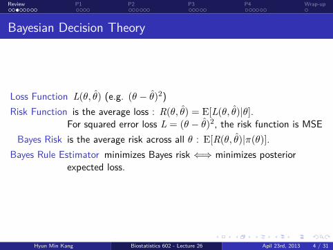
Loss Function L(θ, θ) (e.g. (θ − θ)2)
Risk Function is the average loss : R(θ, θ) = E[L(θ, θ)|θ].For squared error loss L = (θ − θ)2, the risk function is MSE
Bayes Risk is the average risk across all θ : E[R(θ, θ)|π(θ)].Bayes Rule Estimator minimizes Bayes risk ⇐⇒ minimizes posterior
expected loss.
Hyun Min Kang Biostatistics 602 - Lecture 26 Apil 23rd, 2013 4 / 31
..........
.....
......
.....
.....
.....
......
.....
.....
.....
......
.....
.....
.....
......
.....
......
.....
.....
.
. . . . . . . .Review
. . . .P1
. . . . . .P2
. . . . .P3
. . . . . .P4
.Wrap-up
Bayesian Decision Theory
Loss Function L(θ, θ) (e.g. (θ − θ)2)Risk Function is the average loss : R(θ, θ) = E[L(θ, θ)|θ].
For squared error loss L = (θ − θ)2, the risk function is MSEBayes Risk is the average risk across all θ : E[R(θ, θ)|π(θ)].
Bayes Rule Estimator minimizes Bayes risk ⇐⇒ minimizes posteriorexpected loss.
Hyun Min Kang Biostatistics 602 - Lecture 26 Apil 23rd, 2013 4 / 31
..........
.....
......
.....
.....
.....
......
.....
.....
.....
......
.....
.....
.....
......
.....
......
.....
.....
.
. . . . . . . .Review
. . . .P1
. . . . . .P2
. . . . .P3
. . . . . .P4
.Wrap-up
Bayesian Decision Theory
Loss Function L(θ, θ) (e.g. (θ − θ)2)Risk Function is the average loss : R(θ, θ) = E[L(θ, θ)|θ].
For squared error loss L = (θ − θ)2, the risk function is MSE
Bayes Risk is the average risk across all θ : E[R(θ, θ)|π(θ)].Bayes Rule Estimator minimizes Bayes risk ⇐⇒ minimizes posterior
expected loss.
Hyun Min Kang Biostatistics 602 - Lecture 26 Apil 23rd, 2013 4 / 31
..........
.....
......
.....
.....
.....
......
.....
.....
.....
......
.....
.....
.....
......
.....
......
.....
.....
.
. . . . . . . .Review
. . . .P1
. . . . . .P2
. . . . .P3
. . . . . .P4
.Wrap-up
Bayesian Decision Theory
Loss Function L(θ, θ) (e.g. (θ − θ)2)Risk Function is the average loss : R(θ, θ) = E[L(θ, θ)|θ].
For squared error loss L = (θ − θ)2, the risk function is MSEBayes Risk is the average risk across all θ : E[R(θ, θ)|π(θ)].
Bayes Rule Estimator minimizes Bayes risk ⇐⇒ minimizes posteriorexpected loss.
Hyun Min Kang Biostatistics 602 - Lecture 26 Apil 23rd, 2013 4 / 31
..........
.....
......
.....
.....
.....
......
.....
.....
.....
......
.....
.....
.....
......
.....
......
.....
.....
.
. . . . . . . .Review
. . . .P1
. . . . . .P2
. . . . .P3
. . . . . .P4
.Wrap-up
Bayesian Decision Theory
Loss Function L(θ, θ) (e.g. (θ − θ)2)Risk Function is the average loss : R(θ, θ) = E[L(θ, θ)|θ].
For squared error loss L = (θ − θ)2, the risk function is MSEBayes Risk is the average risk across all θ : E[R(θ, θ)|π(θ)].
Bayes Rule Estimator minimizes Bayes risk ⇐⇒ minimizes posteriorexpected loss.
Hyun Min Kang Biostatistics 602 - Lecture 26 Apil 23rd, 2013 4 / 31

..........
.....
......
.....
.....
.....
......
.....
.....
.....
......
.....
.....
.....
......
.....
......
.....
.....
.
. . . . . . . .Review
. . . .P1
. . . . . .P2
. . . . .P3
. . . . . .P4
.Wrap-up
Asymptotics
Consistency Using law of large numbers, show variance and biasconverges to zero, for any continuous mapping function τ
Asymptotic Normality Using central limit theorem, Slutsky Theorem, andDelta Method
Asymptotic Relative Efficiency ARE(Vn,Wn) = σ2W/σ2
V.Asymptotically Efficient ARE with CR-bound of unbiased estimator of
τ(θ) is 1.Asymptotic Efficiency of MLE Theorem 10.1.12 MLE is always
asymptotically efficient under regularity condition.
Hyun Min Kang Biostatistics 602 - Lecture 26 Apil 23rd, 2013 5 / 31

..........
.....
......
.....
.....
.....
......
.....
.....
.....
......
.....
.....
.....
......
.....
......
.....
.....
.
. . . . . . . .Review
. . . .P1
. . . . . .P2
. . . . .P3
. . . . . .P4
.Wrap-up
Asymptotics
Consistency Using law of large numbers, show variance and biasconverges to zero, for any continuous mapping function τ
Asymptotic Normality Using central limit theorem, Slutsky Theorem, andDelta Method
Asymptotic Relative Efficiency ARE(Vn,Wn) = σ2W/σ2
V.
Asymptotically Efficient ARE with CR-bound of unbiased estimator ofτ(θ) is 1.
Asymptotic Efficiency of MLE Theorem 10.1.12 MLE is alwaysasymptotically efficient under regularity condition.
Hyun Min Kang Biostatistics 602 - Lecture 26 Apil 23rd, 2013 5 / 31

..........
.....
......
.....
.....
.....
......
.....
.....
.....
......
.....
.....
.....
......
.....
......
.....
.....
.
. . . . . . . .Review
. . . .P1
. . . . . .P2
. . . . .P3
. . . . . .P4
.Wrap-up
Asymptotics
Consistency Using law of large numbers, show variance and biasconverges to zero, for any continuous mapping function τ
Asymptotic Normality Using central limit theorem, Slutsky Theorem, andDelta Method
Asymptotic Relative Efficiency ARE(Vn,Wn) = σ2W/σ2
V.Asymptotically Efficient ARE with CR-bound of unbiased estimator of
τ(θ) is 1.
Asymptotic Efficiency of MLE Theorem 10.1.12 MLE is alwaysasymptotically efficient under regularity condition.
Hyun Min Kang Biostatistics 602 - Lecture 26 Apil 23rd, 2013 5 / 31

..........
.....
......
.....
.....
.....
......
.....
.....
.....
......
.....
.....
.....
......
.....
......
.....
.....
.
. . . . . . . .Review
. . . .P1
. . . . . .P2
. . . . .P3
. . . . . .P4
.Wrap-up
Asymptotics
Consistency Using law of large numbers, show variance and biasconverges to zero, for any continuous mapping function τ
Asymptotic Normality Using central limit theorem, Slutsky Theorem, andDelta Method
Asymptotic Relative Efficiency ARE(Vn,Wn) = σ2W/σ2
V.Asymptotically Efficient ARE with CR-bound of unbiased estimator of
τ(θ) is 1.Asymptotic Efficiency of MLE Theorem 10.1.12 MLE is always
asymptotically efficient under regularity condition.
Hyun Min Kang Biostatistics 602 - Lecture 26 Apil 23rd, 2013 5 / 31
..........
.....
......
.....
.....
.....
......
.....
.....
.....
......
.....
.....
.....
......
.....
......
.....
.....
.
. . . . . . . .Review
. . . .P1
. . . . . .P2
. . . . .P3
. . . . . .P4
.Wrap-up
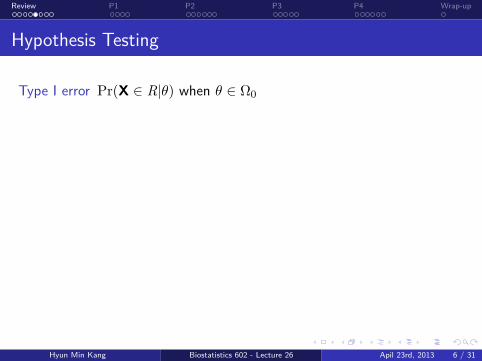
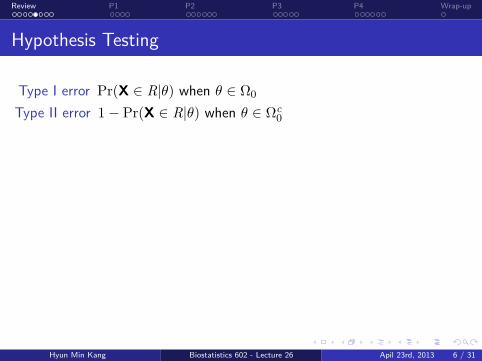
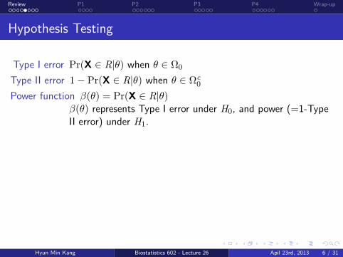
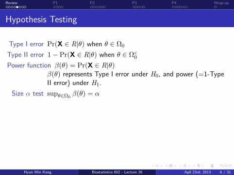
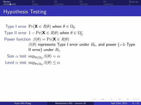
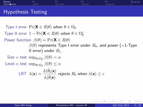
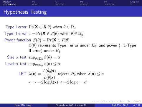
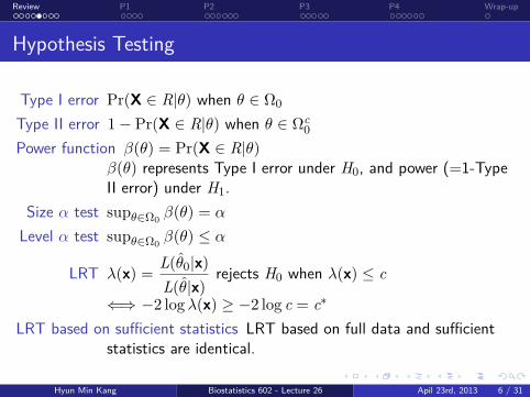
Hypothesis Testing
Type I error Pr(X ∈ R|θ) when θ ∈ Ω0
Type II error 1− Pr(X ∈ R|θ) when θ ∈ Ωc0
Power function β(θ) = Pr(X ∈ R|θ)β(θ) represents Type I error under H0, and power (=1-TypeII error) under H1.
Size α test supθ∈Ω0β(θ) = α
Level α test supθ∈Ω0β(θ) ≤ α
LRT λ(x) = L(θ0|x)L(θ|x)
rejects H0 when λ(x) ≤ c
⇐⇒ −2 logλ(x) ≥ −2 log c = c∗
LRT based on sufficient statistics LRT based on full data and sufficientstatistics are identical.
Hyun Min Kang Biostatistics 602 - Lecture 26 Apil 23rd, 2013 6 / 31
..........
.....
......
.....
.....
.....
......
.....
.....
.....
......
.....
.....
.....
......
.....
......
.....
.....
.
. . . . . . . .Review
. . . .P1
. . . . . .P2
. . . . .P3
. . . . . .P4
.Wrap-up
Hypothesis Testing
Type I error Pr(X ∈ R|θ) when θ ∈ Ω0
Type II error 1− Pr(X ∈ R|θ) when θ ∈ Ωc0
Power function β(θ) = Pr(X ∈ R|θ)β(θ) represents Type I error under H0, and power (=1-TypeII error) under H1.
Size α test supθ∈Ω0β(θ) = α
Level α test supθ∈Ω0β(θ) ≤ α
LRT λ(x) = L(θ0|x)L(θ|x)
rejects H0 when λ(x) ≤ c
⇐⇒ −2 logλ(x) ≥ −2 log c = c∗
LRT based on sufficient statistics LRT based on full data and sufficientstatistics are identical.
Hyun Min Kang Biostatistics 602 - Lecture 26 Apil 23rd, 2013 6 / 31

..........
.....
......
.....
.....
.....
......
.....
.....
.....
......
.....
.....
.....
......
.....
......
.....
.....
.
. . . . . . . .Review
. . . .P1
. . . . . .P2
. . . . .P3
. . . . . .P4
.Wrap-up
Hypothesis Testing
Type I error Pr(X ∈ R|θ) when θ ∈ Ω0
Type II error 1− Pr(X ∈ R|θ) when θ ∈ Ωc0
Power function β(θ) = Pr(X ∈ R|θ)
β(θ) represents Type I error under H0, and power (=1-TypeII error) under H1.
Size α test supθ∈Ω0β(θ) = α
Level α test supθ∈Ω0β(θ) ≤ α
LRT λ(x) = L(θ0|x)L(θ|x)
rejects H0 when λ(x) ≤ c
⇐⇒ −2 logλ(x) ≥ −2 log c = c∗
LRT based on sufficient statistics LRT based on full data and sufficientstatistics are identical.
Hyun Min Kang Biostatistics 602 - Lecture 26 Apil 23rd, 2013 6 / 31
..........
.....
......
.....
.....
.....
......
.....
.....
.....
......
.....
.....
.....
......
.....
......
.....
.....
.
. . . . . . . .Review
. . . .P1
. . . . . .P2
. . . . .P3
. . . . . .P4
.Wrap-up
Hypothesis Testing
Type I error Pr(X ∈ R|θ) when θ ∈ Ω0
Type II error 1− Pr(X ∈ R|θ) when θ ∈ Ωc0
Power function β(θ) = Pr(X ∈ R|θ)β(θ) represents Type I error under H0, and power (=1-TypeII error) under H1.
Size α test supθ∈Ω0β(θ) = α
Level α test supθ∈Ω0β(θ) ≤ α
LRT λ(x) = L(θ0|x)L(θ|x)
rejects H0 when λ(x) ≤ c
⇐⇒ −2 logλ(x) ≥ −2 log c = c∗
LRT based on sufficient statistics LRT based on full data and sufficientstatistics are identical.
Hyun Min Kang Biostatistics 602 - Lecture 26 Apil 23rd, 2013 6 / 31

..........
.....
......
.....
.....
.....
......
.....
.....
.....
......
.....
.....
.....
......
.....
......
.....
.....
.
. . . . . . . .Review
. . . .P1
. . . . . .P2
. . . . .P3
. . . . . .P4
.Wrap-up
UMP
Unbiased Test β(θ1) ≥ β(θ0) for every θ1 ∈ Ωc0 and θ0 ∈ Ω0.
UMP Test β(θ) ≥ β′(θ) for every θ ∈ Ωc0 and β′(θ) of every other test
with a class of test C.UMP level α Test UMP test in the class of all the level α test. (smallest
Type II error given the upper bound of Type I error)Neyman-Pearson For H0 : θ = θ0 vs. H1 : θ = θ1, a test with rejection
region f(x|θ1)/f(x|θ0) > k is a UMP level α test for its size.MLR g(t|θ2)/g(t|θ1) is an increasing function of t for every
θ2 > θ1.Karlin-Rabin If T is sufficient and has MLR, then test rejecting
R = T : T > t0 or R = T : T < t0 is an UMP level αtest for one-sided composite hypothesis.
Hyun Min Kang Biostatistics 602 - Lecture 26 Apil 23rd, 2013 7 / 31

..........
.....
......
.....
.....
.....
......
.....
.....
.....
......
.....
.....
.....
......
.....
......
.....
.....
.
. . . . . . . .Review
. . . .P1
. . . . . .P2
. . . . .P3
. . . . . .P4
.Wrap-up
UMP
Unbiased Test β(θ1) ≥ β(θ0) for every θ1 ∈ Ωc0 and θ0 ∈ Ω0.
UMP Test β(θ) ≥ β′(θ) for every θ ∈ Ωc0 and β′(θ) of every other test
with a class of test C.
UMP level α Test UMP test in the class of all the level α test. (smallestType II error given the upper bound of Type I error)
Neyman-Pearson For H0 : θ = θ0 vs. H1 : θ = θ1, a test with rejectionregion f(x|θ1)/f(x|θ0) > k is a UMP level α test for its size.
MLR g(t|θ2)/g(t|θ1) is an increasing function of t for everyθ2 > θ1.
Karlin-Rabin If T is sufficient and has MLR, then test rejectingR = T : T > t0 or R = T : T < t0 is an UMP level αtest for one-sided composite hypothesis.
Hyun Min Kang Biostatistics 602 - Lecture 26 Apil 23rd, 2013 7 / 31

..........
.....
......
.....
.....
.....
......
.....
.....
.....
......
.....
.....
.....
......
.....
......
.....
.....
.
. . . . . . . .Review
. . . .P1
. . . . . .P2
. . . . .P3
. . . . . .P4
.Wrap-up
UMP
Unbiased Test β(θ1) ≥ β(θ0) for every θ1 ∈ Ωc0 and θ0 ∈ Ω0.
UMP Test β(θ) ≥ β′(θ) for every θ ∈ Ωc0 and β′(θ) of every other test
with a class of test C.UMP level α Test UMP test in the class of all the level α test. (smallest
Type II error given the upper bound of Type I error)
Neyman-Pearson For H0 : θ = θ0 vs. H1 : θ = θ1, a test with rejectionregion f(x|θ1)/f(x|θ0) > k is a UMP level α test for its size.
MLR g(t|θ2)/g(t|θ1) is an increasing function of t for everyθ2 > θ1.
Karlin-Rabin If T is sufficient and has MLR, then test rejectingR = T : T > t0 or R = T : T < t0 is an UMP level αtest for one-sided composite hypothesis.
Hyun Min Kang Biostatistics 602 - Lecture 26 Apil 23rd, 2013 7 / 31

..........
.....
......
.....
.....
.....
......
.....
.....
.....
......
.....
.....
.....
......
.....
......
.....
.....
.
. . . . . . . .Review
. . . .P1
. . . . . .P2
. . . . .P3
. . . . . .P4
.Wrap-up
UMP
Unbiased Test β(θ1) ≥ β(θ0) for every θ1 ∈ Ωc0 and θ0 ∈ Ω0.
UMP Test β(θ) ≥ β′(θ) for every θ ∈ Ωc0 and β′(θ) of every other test
with a class of test C.UMP level α Test UMP test in the class of all the level α test. (smallest
Type II error given the upper bound of Type I error)Neyman-Pearson For H0 : θ = θ0 vs. H1 : θ = θ1, a test with rejection
region f(x|θ1)/f(x|θ0) > k is a UMP level α test for its size.
MLR g(t|θ2)/g(t|θ1) is an increasing function of t for everyθ2 > θ1.
Karlin-Rabin If T is sufficient and has MLR, then test rejectingR = T : T > t0 or R = T : T < t0 is an UMP level αtest for one-sided composite hypothesis.
Hyun Min Kang Biostatistics 602 - Lecture 26 Apil 23rd, 2013 7 / 31

..........
.....
......
.....
.....
.....
......
.....
.....
.....
......
.....
.....
.....
......
.....
......
.....
.....
.
. . . . . . . .Review
. . . .P1
. . . . . .P2
. . . . .P3
. . . . . .P4
.Wrap-up
UMP
Unbiased Test β(θ1) ≥ β(θ0) for every θ1 ∈ Ωc0 and θ0 ∈ Ω0.
UMP Test β(θ) ≥ β′(θ) for every θ ∈ Ωc0 and β′(θ) of every other test
with a class of test C.UMP level α Test UMP test in the class of all the level α test. (smallest
Type II error given the upper bound of Type I error)Neyman-Pearson For H0 : θ = θ0 vs. H1 : θ = θ1, a test with rejection
region f(x|θ1)/f(x|θ0) > k is a UMP level α test for its size.MLR g(t|θ2)/g(t|θ1) is an increasing function of t for every
θ2 > θ1.
Karlin-Rabin If T is sufficient and has MLR, then test rejectingR = T : T > t0 or R = T : T < t0 is an UMP level αtest for one-sided composite hypothesis.
Hyun Min Kang Biostatistics 602 - Lecture 26 Apil 23rd, 2013 7 / 31

..........
.....
......
.....
.....
.....
......
.....
.....
.....
......
.....
.....
.....
......
.....
......
.....
.....
.
. . . . . . . .Review
. . . .P1
. . . . . .P2
. . . . .P3
. . . . . .P4
.Wrap-up
UMP
Unbiased Test β(θ1) ≥ β(θ0) for every θ1 ∈ Ωc0 and θ0 ∈ Ω0.
UMP Test β(θ) ≥ β′(θ) for every θ ∈ Ωc0 and β′(θ) of every other test
with a class of test C.UMP level α Test UMP test in the class of all the level α test. (smallest
Type II error given the upper bound of Type I error)Neyman-Pearson For H0 : θ = θ0 vs. H1 : θ = θ1, a test with rejection
region f(x|θ1)/f(x|θ0) > k is a UMP level α test for its size.MLR g(t|θ2)/g(t|θ1) is an increasing function of t for every
θ2 > θ1.Karlin-Rabin If T is sufficient and has MLR, then test rejecting
R = T : T > t0 or R = T : T < t0 is an UMP level αtest for one-sided composite hypothesis.
Hyun Min Kang Biostatistics 602 - Lecture 26 Apil 23rd, 2013 7 / 31
..........
.....
......
.....
.....
.....
......
.....
.....
.....
......
.....
.....
.....
......
.....
......
.....
.....
.
. . . . . . . .Review
. . . .P1
. . . . . .P2
. . . . .P3
. . . . . .P4
.Wrap-up
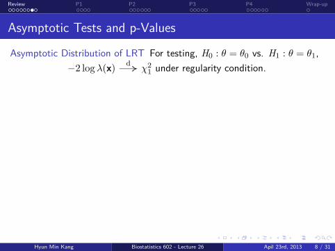
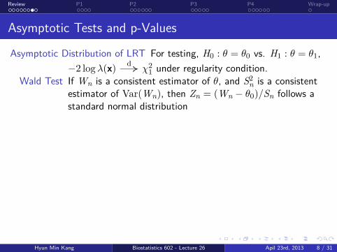
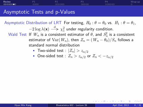
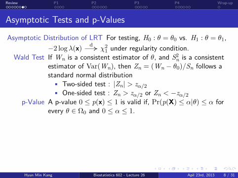
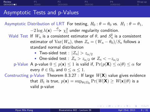
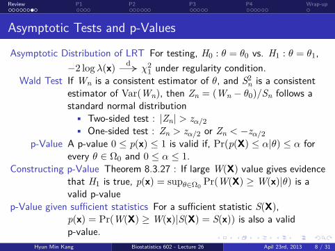
Asymptotic Tests and p-Values
Asymptotic Distribution of LRT For testing, H0 : θ = θ0 vs. H1 : θ = θ1,−2 logλ(x) d→ χ2
1 under regularity condition.
Wald Test If Wn is a consistent estimator of θ, and S2n is a consistent
estimator of Var(Wn), then Zn = (Wn − θ0)/Sn follows astandard normal distribution
• Two-sided test : |Zn| > zα/2• One-sided test : Zn > zα/2 or Zn < −zα/2
p-Value A p-value 0 ≤ p(x) ≤ 1 is valid if, Pr(p(X) ≤ α|θ) ≤ α forevery θ ∈ Ω0 and 0 ≤ α ≤ 1.
Constructing p-Value Theorem 8.3.27 : If large W(X) value gives evidencethat H1 is true, p(x) = supθ∈Ω0
Pr(W(X) ≥ W(x)|θ) is avalid p-value
p-Value given sufficient statistics For a sufficient statistic S(X),p(x) = Pr(W(X) ≥ W(x)|S(X) = S(x)) is also a validp-value.
Hyun Min Kang Biostatistics 602 - Lecture 26 Apil 23rd, 2013 8 / 31
..........
.....
......
.....
.....
.....
......
.....
.....
.....
......
.....
.....
.....
......
.....
......
.....
.....
.
. . . . . . . .Review
. . . .P1
. . . . . .P2
. . . . .P3
. . . . . .P4
.Wrap-up
Asymptotic Tests and p-Values
Asymptotic Distribution of LRT For testing, H0 : θ = θ0 vs. H1 : θ = θ1,−2 logλ(x) d→ χ2
1 under regularity condition.Wald Test If Wn is a consistent estimator of θ, and S2
n is a consistentestimator of Var(Wn), then Zn = (Wn − θ0)/Sn follows astandard normal distribution
• Two-sided test : |Zn| > zα/2• One-sided test : Zn > zα/2 or Zn < −zα/2
p-Value A p-value 0 ≤ p(x) ≤ 1 is valid if, Pr(p(X) ≤ α|θ) ≤ α forevery θ ∈ Ω0 and 0 ≤ α ≤ 1.
Constructing p-Value Theorem 8.3.27 : If large W(X) value gives evidencethat H1 is true, p(x) = supθ∈Ω0
Pr(W(X) ≥ W(x)|θ) is avalid p-value
p-Value given sufficient statistics For a sufficient statistic S(X),p(x) = Pr(W(X) ≥ W(x)|S(X) = S(x)) is also a validp-value.
Hyun Min Kang Biostatistics 602 - Lecture 26 Apil 23rd, 2013 8 / 31

..........
.....
......
.....
.....
.....
......
.....
.....
.....
......
.....
.....
.....
......
.....
......
.....
.....
.
. . . . . . . .Review
. . . .P1
. . . . . .P2
. . . . .P3
. . . . . .P4
.Wrap-up
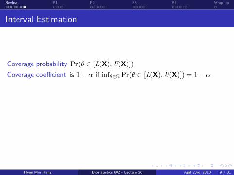
Interval Estimation
Coverage probability Pr(θ ∈ [L(X),U(X)])
Coverage coefficient is 1− α if infθ∈Ω Pr(θ ∈ [L(X),U(X)]) = 1− α
Confidence interval [L(X),U(X)]) is 1− α ifinfθ∈Ω Pr(θ ∈ [L(X),U(X)]) = 1− α
Inverting a level α test If A(θ0) is the acceptance region of a level α test,then C(X) = θ : X ∈ A(θ) is a 1− α confidence set (orinterval).
Hyun Min Kang Biostatistics 602 - Lecture 26 Apil 23rd, 2013 9 / 31
..........
.....
......
.....
.....
.....
......
.....
.....
.....
......
.....
.....
.....
......
.....
......
.....
.....
.
. . . . . . . .Review
. . . .P1
. . . . . .P2
. . . . .P3
. . . . . .P4
.Wrap-up
Interval Estimation
Coverage probability Pr(θ ∈ [L(X),U(X)])
Coverage coefficient is 1− α if infθ∈Ω Pr(θ ∈ [L(X),U(X)]) = 1− α
Confidence interval [L(X),U(X)]) is 1− α ifinfθ∈Ω Pr(θ ∈ [L(X),U(X)]) = 1− α
Inverting a level α test If A(θ0) is the acceptance region of a level α test,then C(X) = θ : X ∈ A(θ) is a 1− α confidence set (orinterval).
Hyun Min Kang Biostatistics 602 - Lecture 26 Apil 23rd, 2013 9 / 31
..........
.....
......
.....
.....
.....
......
.....
.....
.....
......
.....
.....
.....
......
.....
......
.....
.....
.
. . . . . . . .Review
. . . .P1
. . . . . .P2
. . . . .P3
. . . . . .P4
.Wrap-up
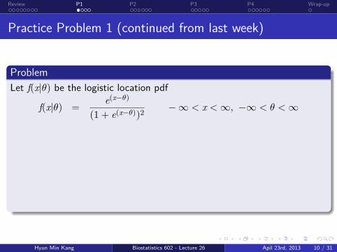
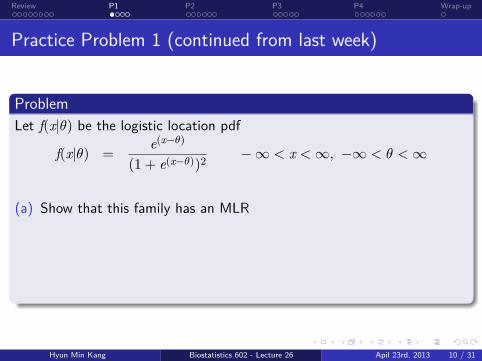
Practice Problem 1 (continued from last week)
.Problem..
......
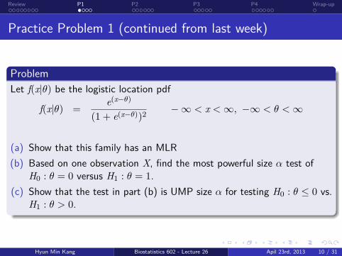
Let f(x|θ) be the logistic location pdf
f(x|θ) =e(x−θ)
(1 + e(x−θ))2−∞ < x < ∞, −∞ < θ < ∞
(a) Show that this family has an MLR(b) Based on one observation X, find the most powerful size α test of
H0 : θ = 0 versus H1 : θ = 1.(c) Show that the test in part (b) is UMP size α for testing H0 : θ ≤ 0 vs.
H1 : θ > 0.
Hyun Min Kang Biostatistics 602 - Lecture 26 Apil 23rd, 2013 10 / 31
..........
.....
......
.....
.....
.....
......
.....
.....
.....
......
.....
.....
.....
......
.....
......
.....
.....
.
. . . . . . . .Review
. . . .P1
. . . . . .P2
. . . . .P3
. . . . . .P4
.Wrap-up
Practice Problem 1 (continued from last week)
.Problem..
......
Let f(x|θ) be the logistic location pdf
f(x|θ) =e(x−θ)
(1 + e(x−θ))2−∞ < x < ∞, −∞ < θ < ∞
(a) Show that this family has an MLR
(b) Based on one observation X, find the most powerful size α test ofH0 : θ = 0 versus H1 : θ = 1.
(c) Show that the test in part (b) is UMP size α for testing H0 : θ ≤ 0 vs.H1 : θ > 0.
Hyun Min Kang Biostatistics 602 - Lecture 26 Apil 23rd, 2013 10 / 31

..........
.....
......
.....
.....
.....
......
.....
.....
.....
......
.....
.....
.....
......
.....
......
.....
.....
.
. . . . . . . .Review
. . . .P1
. . . . . .P2
. . . . .P3
. . . . . .P4
.Wrap-up
Practice Problem 1 (continued from last week)
.Problem..
......
Let f(x|θ) be the logistic location pdf
f(x|θ) =e(x−θ)
(1 + e(x−θ))2−∞ < x < ∞, −∞ < θ < ∞
(a) Show that this family has an MLR(b) Based on one observation X, find the most powerful size α test of
H0 : θ = 0 versus H1 : θ = 1.
(c) Show that the test in part (b) is UMP size α for testing H0 : θ ≤ 0 vs.H1 : θ > 0.
Hyun Min Kang Biostatistics 602 - Lecture 26 Apil 23rd, 2013 10 / 31
..........
.....
......
.....
.....
.....
......
.....
.....
.....
......
.....
.....
.....
......
.....
......
.....
.....
.
. . . . . . . .Review
. . . .P1
. . . . . .P2
. . . . .P3
. . . . . .P4
.Wrap-up
Practice Problem 1 (continued from last week)
.Problem..
......
Let f(x|θ) be the logistic location pdf
f(x|θ) =e(x−θ)
(1 + e(x−θ))2−∞ < x < ∞, −∞ < θ < ∞
(a) Show that this family has an MLR(b) Based on one observation X, find the most powerful size α test of
H0 : θ = 0 versus H1 : θ = 1.(c) Show that the test in part (b) is UMP size α for testing H0 : θ ≤ 0 vs.
H1 : θ > 0.
Hyun Min Kang Biostatistics 602 - Lecture 26 Apil 23rd, 2013 10 / 31

..........
.....
......
.....
.....
.....
......
.....
.....
.....
......
.....
.....
.....
......
.....
......
.....
.....
.
. . . . . . . .Review
. . . .P1
. . . . . .P2
. . . . .P3
. . . . . .P4
.Wrap-up
Solution for (a)For θ1 < θ2,
f(x|θ2)f(x|θ1)
=
e(x−θ2)
(1+e(x−θ2))2
e(x−θ1)
(1+e(x−θ1))2
= e(θ1−θ2)
(1 + e(x−θ1)
1 + e(x−θ2)
)2
Let r(x) = (1 + ex−θ1)/(1 + ex−θ2)
r′(x) =e(x−θ1)(1 + e(x−θ2))− (1 + e(x−θ1))e(x−θ2)
(1 + e(x−θ2))2
=e(x−θ1) − e(x−θ2)
(1 + e(x−θ2))2> 0 (∵ x − θ1 > x − θ2)
Therefore, the family of X has an MLR.
Hyun Min Kang Biostatistics 602 - Lecture 26 Apil 23rd, 2013 11 / 31

..........
.....
......
.....
.....
.....
......
.....
.....
.....
......
.....
.....
.....
......
.....
......
.....
.....
.
. . . . . . . .Review
. . . .P1
. . . . . .P2
. . . . .P3
. . . . . .P4
.Wrap-up
Solution for (a)For θ1 < θ2,
f(x|θ2)f(x|θ1)
=
e(x−θ2)
(1+e(x−θ2))2
e(x−θ1)
(1+e(x−θ1))2
= e(θ1−θ2)
(1 + e(x−θ1)
1 + e(x−θ2)
)2
Let r(x) = (1 + ex−θ1)/(1 + ex−θ2)
r′(x) =e(x−θ1)(1 + e(x−θ2))− (1 + e(x−θ1))e(x−θ2)
(1 + e(x−θ2))2
=e(x−θ1) − e(x−θ2)
(1 + e(x−θ2))2> 0 (∵ x − θ1 > x − θ2)
Therefore, the family of X has an MLR.Hyun Min Kang Biostatistics 602 - Lecture 26 Apil 23rd, 2013 11 / 31

..........
.....
......
.....
.....
.....
......
.....
.....
.....
......
.....
.....
.....
......
.....
......
.....
.....
.
. . . . . . . .Review
. . . .P1
. . . . . .P2
. . . . .P3
. . . . . .P4
.Wrap-up
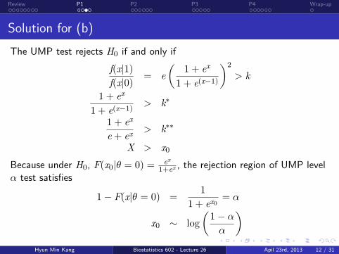
Solution for (b)The UMP test rejects H0 if and only if
f(x|1)f(x|0) = e
(1 + ex
1 + e(x−1)
)2
> k
1 + ex
1 + e(x−1)> k∗
1 + ex
e + ex > k∗∗
X > x0Because under H0, F(x0|θ = 0) = ex
1+ex , the rejection region of UMP levelα test satisfies
1− F(x|θ = 0) =1
1 + ex0 = α
x0 ∼ log(1− α
α
)
Hyun Min Kang Biostatistics 602 - Lecture 26 Apil 23rd, 2013 12 / 31

..........
.....
......
.....
.....
.....
......
.....
.....
.....
......
.....
.....
.....
......
.....
......
.....
.....
.
. . . . . . . .Review
. . . .P1
. . . . . .P2
. . . . .P3
. . . . . .P4
.Wrap-up
Solution for (b)The UMP test rejects H0 if and only if
f(x|1)f(x|0) = e
(1 + ex
1 + e(x−1)
)2
> k
1 + ex
1 + e(x−1)> k∗
1 + ex
e + ex > k∗∗
X > x0
Because under H0, F(x0|θ = 0) = ex
1+ex , the rejection region of UMP levelα test satisfies
1− F(x|θ = 0) =1
1 + ex0 = α
x0 ∼ log(1− α
α
)
Hyun Min Kang Biostatistics 602 - Lecture 26 Apil 23rd, 2013 12 / 31
..........
.....
......
.....
.....
.....
......
.....
.....
.....
......
.....
.....
.....
......
.....
......
.....
.....
.
. . . . . . . .Review
. . . .P1
. . . . . .P2
. . . . .P3
. . . . . .P4
.Wrap-up
Solution for (b)The UMP test rejects H0 if and only if
f(x|1)f(x|0) = e
(1 + ex
1 + e(x−1)
)2
> k
1 + ex
1 + e(x−1)> k∗
1 + ex
e + ex > k∗∗
X > x0Because under H0, F(x0|θ = 0) = ex
1+ex , the rejection region of UMP levelα test satisfies
1− F(x|θ = 0) =1
1 + ex0 = α
x0 ∼ log(1− α
α
)Hyun Min Kang Biostatistics 602 - Lecture 26 Apil 23rd, 2013 12 / 31

..........
.....
......
.....
.....
.....
......
.....
.....
.....
......
.....
.....
.....
......
.....
......
.....
.....
.
. . . . . . . .Review
. . . .P1
. . . . . .P2
. . . . .P3
. . . . . .P4
.Wrap-up
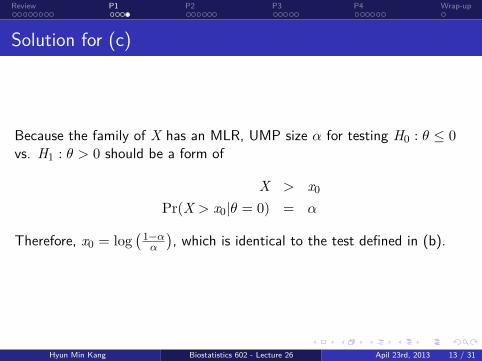
Solution for (c)
Because the family of X has an MLR, UMP size α for testing H0 : θ ≤ 0vs. H1 : θ > 0 should be a form of
X > x0Pr(X > x0|θ = 0) = α
Therefore, x0 = log(1−αα
), which is identical to the test defined in (b).
Hyun Min Kang Biostatistics 602 - Lecture 26 Apil 23rd, 2013 13 / 31
..........
.....
......
.....
.....
.....
......
.....
.....
.....
......
.....
.....
.....
......
.....
......
.....
.....
.
. . . . . . . .Review
. . . .P1
. . . . . .P2
. . . . .P3
. . . . . .P4
.Wrap-up
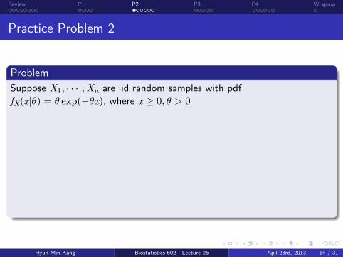
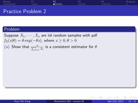
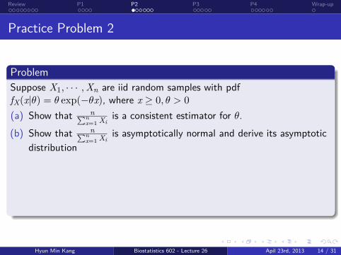
Practice Problem 2
.Problem..
......
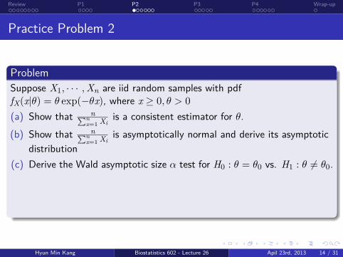
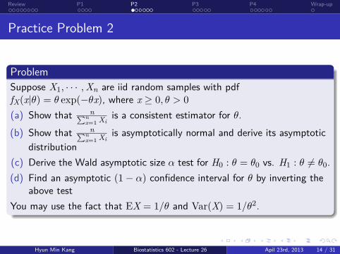
Suppose X1, · · · ,Xn are iid random samples with pdffX(x|θ) = θ exp(−θx), where x ≥ 0, θ > 0
(a) Show that n∑nx=1 Xi
is a consistent estimator for θ.(b) Show that n∑n
x=1 Xiis asymptotically normal and derive its asymptotic
distribution(c) Derive the Wald asymptotic size α test for H0 : θ = θ0 vs. H1 : θ = θ0.(d) Find an asymptotic (1− α) confidence interval for θ by inverting the
above testYou may use the fact that EX = 1/θ and Var(X) = 1/θ2.
Hyun Min Kang Biostatistics 602 - Lecture 26 Apil 23rd, 2013 14 / 31
..........
.....
......
.....
.....
.....
......
.....
.....
.....
......
.....
.....
.....
......
.....
......
.....
.....
.
. . . . . . . .Review
. . . .P1
. . . . . .P2
. . . . .P3
. . . . . .P4
.Wrap-up
Practice Problem 2
.Problem..
......
Suppose X1, · · · ,Xn are iid random samples with pdffX(x|θ) = θ exp(−θx), where x ≥ 0, θ > 0
(a) Show that n∑nx=1 Xi
is a consistent estimator for θ.
(b) Show that n∑nx=1 Xi
is asymptotically normal and derive its asymptoticdistribution
(c) Derive the Wald asymptotic size α test for H0 : θ = θ0 vs. H1 : θ = θ0.(d) Find an asymptotic (1− α) confidence interval for θ by inverting the
above testYou may use the fact that EX = 1/θ and Var(X) = 1/θ2.
Hyun Min Kang Biostatistics 602 - Lecture 26 Apil 23rd, 2013 14 / 31
..........
.....
......
.....
.....
.....
......
.....
.....
.....
......
.....
.....
.....
......
.....
......
.....
.....
.
. . . . . . . .Review
. . . .P1
. . . . . .P2
. . . . .P3
. . . . . .P4
.Wrap-up
Practice Problem 2
.Problem..
......
Suppose X1, · · · ,Xn are iid random samples with pdffX(x|θ) = θ exp(−θx), where x ≥ 0, θ > 0
(a) Show that n∑nx=1 Xi
is a consistent estimator for θ.(b) Show that n∑n
x=1 Xiis asymptotically normal and derive its asymptotic
distribution
(c) Derive the Wald asymptotic size α test for H0 : θ = θ0 vs. H1 : θ = θ0.(d) Find an asymptotic (1− α) confidence interval for θ by inverting the
above testYou may use the fact that EX = 1/θ and Var(X) = 1/θ2.
Hyun Min Kang Biostatistics 602 - Lecture 26 Apil 23rd, 2013 14 / 31
..........
.....
......
.....
.....
.....
......
.....
.....
.....
......
.....
.....
.....
......
.....
......
.....
.....
.
. . . . . . . .Review
. . . .P1
. . . . . .P2
. . . . .P3
. . . . . .P4
.Wrap-up
Practice Problem 2
.Problem..
......
Suppose X1, · · · ,Xn are iid random samples with pdffX(x|θ) = θ exp(−θx), where x ≥ 0, θ > 0
(a) Show that n∑nx=1 Xi
is a consistent estimator for θ.(b) Show that n∑n
x=1 Xiis asymptotically normal and derive its asymptotic
distribution(c) Derive the Wald asymptotic size α test for H0 : θ = θ0 vs. H1 : θ = θ0.
(d) Find an asymptotic (1− α) confidence interval for θ by inverting theabove test
You may use the fact that EX = 1/θ and Var(X) = 1/θ2.
Hyun Min Kang Biostatistics 602 - Lecture 26 Apil 23rd, 2013 14 / 31
..........
.....
......
.....
.....
.....
......
.....
.....
.....
......
.....
.....
.....
......
.....
......
.....
.....
.
. . . . . . . .Review
. . . .P1
. . . . . .P2
. . . . .P3
. . . . . .P4
.Wrap-up
Practice Problem 2
.Problem..
......
Suppose X1, · · · ,Xn are iid random samples with pdffX(x|θ) = θ exp(−θx), where x ≥ 0, θ > 0
(a) Show that n∑nx=1 Xi
is a consistent estimator for θ.(b) Show that n∑n
x=1 Xiis asymptotically normal and derive its asymptotic
distribution(c) Derive the Wald asymptotic size α test for H0 : θ = θ0 vs. H1 : θ = θ0.(d) Find an asymptotic (1− α) confidence interval for θ by inverting the
above testYou may use the fact that EX = 1/θ and Var(X) = 1/θ2.
Hyun Min Kang Biostatistics 602 - Lecture 26 Apil 23rd, 2013 14 / 31

..........
.....
......
.....
.....
.....
......
.....
.....
.....
......
.....
.....
.....
......
.....
......
.....
.....
.
. . . . . . . .Review
. . . .P1
. . . . . .P2
. . . . .P3
. . . . . .P4
.Wrap-up
Solution (a) - Consistency
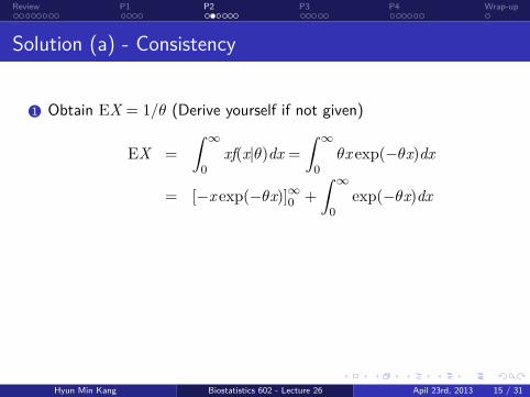
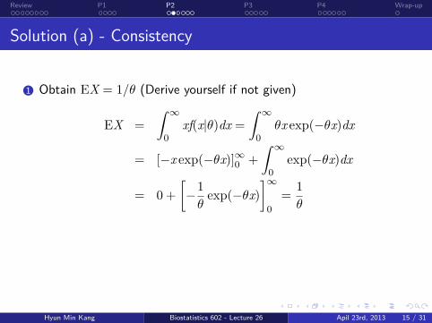
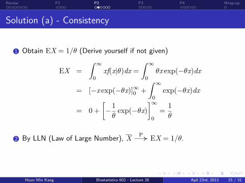
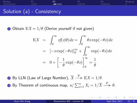
..1 Obtain EX = 1/θ (Derive yourself if not given)
EX =
∫ ∞
0xf(x|θ)dx =
∫ ∞
0θx exp(−θx)dx
= [−x exp(−θx)]∞0 +
∫ ∞
0exp(−θx)dx
= 0 +
[−1
θexp(−θx)
]∞0
=1
θ
..2 By LLN (Law of Large Number), X P→ EX = 1/θ.
..3 By Theorem of continuous map, n/∑n
i=1 Xi = 1/X P→ θ.
Hyun Min Kang Biostatistics 602 - Lecture 26 Apil 23rd, 2013 15 / 31
..........
.....
......
.....
.....
.....
......
.....
.....
.....
......
.....
.....
.....
......
.....
......
.....
.....
.
. . . . . . . .Review
. . . .P1
. . . . . .P2
. . . . .P3
. . . . . .P4
.Wrap-up
Solution (a) - Consistency
..1 Obtain EX = 1/θ (Derive yourself if not given)
EX =
∫ ∞
0xf(x|θ)dx =
∫ ∞
0θx exp(−θx)dx
= [−x exp(−θx)]∞0 +
∫ ∞
0exp(−θx)dx
= 0 +
[−1
θexp(−θx)
]∞0
=1
θ
..2 By LLN (Law of Large Number), X P→ EX = 1/θ.
..3 By Theorem of continuous map, n/∑n
i=1 Xi = 1/X P→ θ.
Hyun Min Kang Biostatistics 602 - Lecture 26 Apil 23rd, 2013 15 / 31

..........
.....
......
.....
.....
.....
......
.....
.....
.....
......
.....
.....
.....
......
.....
......
.....
.....
.
. . . . . . . .Review
. . . .P1
. . . . . .P2
. . . . .P3
. . . . . .P4
.Wrap-up
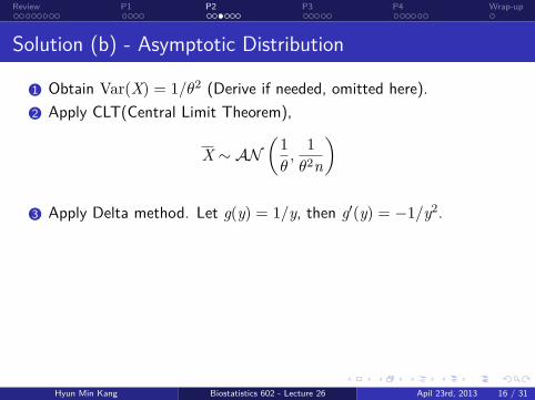
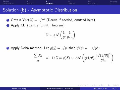
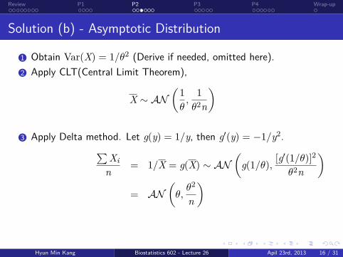
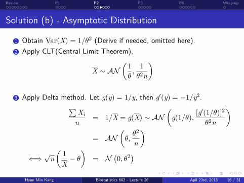
Solution (b) - Asymptotic Distribution
..1 Obtain Var(X) = 1/θ2 (Derive if needed, omitted here).
..2 Apply CLT(Central Limit Theorem),
X ∼ AN(1
θ,
1
θ2n
)
..3 Apply Delta method. Let g(y) = 1/y, then g′(y) = −1/y2.∑Xi
n = 1/X = g(X) ∼ AN(
g(1/θ), [g′(1/θ)]2
θ2n
)= AN
(θ,
θ2
n
)⇐⇒
√n(1
X− θ
)= N
(0, θ2
)
Hyun Min Kang Biostatistics 602 - Lecture 26 Apil 23rd, 2013 16 / 31

..........
.....
......
.....
.....
.....
......
.....
.....
.....
......
.....
.....
.....
......
.....
......
.....
.....
.
. . . . . . . .Review
. . . .P1
. . . . . .P2
. . . . .P3
. . . . . .P4
.Wrap-up
Solution (b) - Asymptotic Distribution
..1 Obtain Var(X) = 1/θ2 (Derive if needed, omitted here).
..2 Apply CLT(Central Limit Theorem),
X ∼ AN(1
θ,
1
θ2n
)
..3 Apply Delta method. Let g(y) = 1/y, then g′(y) = −1/y2.∑Xi
n = 1/X = g(X) ∼ AN(
g(1/θ), [g′(1/θ)]2
θ2n
)= AN
(θ,
θ2
n
)⇐⇒
√n(1
X− θ
)= N
(0, θ2
)
Hyun Min Kang Biostatistics 602 - Lecture 26 Apil 23rd, 2013 16 / 31
..........
.....
......
.....
.....
.....
......
.....
.....
.....
......
.....
.....
.....
......
.....
......
.....
.....
.
. . . . . . . .Review
. . . .P1
. . . . . .P2
. . . . .P3
. . . . . .P4
.Wrap-up
Solution (b) - Asymptotic Distribution
..1 Obtain Var(X) = 1/θ2 (Derive if needed, omitted here).
..2 Apply CLT(Central Limit Theorem),
X ∼ AN(1
θ,
1
θ2n
)
..3 Apply Delta method. Let g(y) = 1/y, then g′(y) = −1/y2.
∑Xi
n = 1/X = g(X) ∼ AN(
g(1/θ), [g′(1/θ)]2
θ2n
)= AN
(θ,
θ2
n
)⇐⇒
√n(1
X− θ
)= N
(0, θ2
)
Hyun Min Kang Biostatistics 602 - Lecture 26 Apil 23rd, 2013 16 / 31
..........
.....
......
.....
.....
.....
......
.....
.....
.....
......
.....
.....
.....
......
.....
......
.....
.....
.
. . . . . . . .Review
. . . .P1
. . . . . .P2
. . . . .P3
. . . . . .P4
.Wrap-up
Solution (b) - Asymptotic Distribution
..1 Obtain Var(X) = 1/θ2 (Derive if needed, omitted here).
..2 Apply CLT(Central Limit Theorem),
X ∼ AN(1
θ,
1
θ2n
)
..3 Apply Delta method. Let g(y) = 1/y, then g′(y) = −1/y2.∑Xi
n = 1/X = g(X) ∼ AN(
g(1/θ), [g′(1/θ)]2
θ2n
)
= AN(θ,
θ2
n
)⇐⇒
√n(1
X− θ
)= N
(0, θ2
)
Hyun Min Kang Biostatistics 602 - Lecture 26 Apil 23rd, 2013 16 / 31
..........
.....
......
.....
.....
.....
......
.....
.....
.....
......
.....
.....
.....
......
.....
......
.....
.....
.
. . . . . . . .Review
. . . .P1
. . . . . .P2
. . . . .P3
. . . . . .P4
.Wrap-up
Solution (b) - Asymptotic Distribution
..1 Obtain Var(X) = 1/θ2 (Derive if needed, omitted here).
..2 Apply CLT(Central Limit Theorem),
X ∼ AN(1
θ,
1
θ2n
)
..3 Apply Delta method. Let g(y) = 1/y, then g′(y) = −1/y2.∑Xi
n = 1/X = g(X) ∼ AN(
g(1/θ), [g′(1/θ)]2
θ2n
)= AN
(θ,
θ2
n
)
⇐⇒√
n(1
X− θ
)= N
(0, θ2
)
Hyun Min Kang Biostatistics 602 - Lecture 26 Apil 23rd, 2013 16 / 31
..........
.....
......
.....
.....
.....
......
.....
.....
.....
......
.....
.....
.....
......
.....
......
.....
.....
.
. . . . . . . .Review
. . . .P1
. . . . . .P2
. . . . .P3
. . . . . .P4
.Wrap-up
Solution (b) - Asymptotic Distribution
..1 Obtain Var(X) = 1/θ2 (Derive if needed, omitted here).
..2 Apply CLT(Central Limit Theorem),
X ∼ AN(1
θ,
1
θ2n
)
..3 Apply Delta method. Let g(y) = 1/y, then g′(y) = −1/y2.∑Xi
n = 1/X = g(X) ∼ AN(
g(1/θ), [g′(1/θ)]2
θ2n
)= AN
(θ,
θ2
n
)⇐⇒
√n(1
X− θ
)= N
(0, θ2
)Hyun Min Kang Biostatistics 602 - Lecture 26 Apil 23rd, 2013 16 / 31

..........
.....
......
.....
.....
.....
......
.....
.....
.....
......
.....
.....
.....
......
.....
......
.....
.....
.
. . . . . . . .Review
. . . .P1
. . . . . .P2
. . . . .P3
. . . . . .P4
.Wrap-up
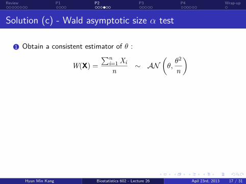
Solution (c) - Wald asymptotic size α test
..1 Obtain a consistent estimator of θ :
W(X) =
∑ni=1 Xin ∼ AN
(θ,
θ2
n
)..2 Obtain a constant estimator of Var(W)
1
n − 1
n∑i=1
(Xi − X)2P→ Var(X) =
1
θ2(CLT)
n − 1∑ni=1(Xi − X)2
P→ θ2 (Continuous Map Theorem).
S2 =n∑n
i=1(Xi − X)2P→ θ2 (Slutsky’s Theorem).
Hyun Min Kang Biostatistics 602 - Lecture 26 Apil 23rd, 2013 17 / 31
..........
.....
......
.....
.....
.....
......
.....
.....
.....
......
.....
.....
.....
......
.....
......
.....
.....
.
. . . . . . . .Review
. . . .P1
. . . . . .P2
. . . . .P3
. . . . . .P4
.Wrap-up
Solution (c) - Wald asymptotic size α test
..1 Obtain a consistent estimator of θ :
W(X) =
∑ni=1 Xin ∼ AN
(θ,
θ2
n
)
..2 Obtain a constant estimator of Var(W)
1
n − 1
n∑i=1
(Xi − X)2P→ Var(X) =
1
θ2(CLT)
n − 1∑ni=1(Xi − X)2
P→ θ2 (Continuous Map Theorem).
S2 =n∑n
i=1(Xi − X)2P→ θ2 (Slutsky’s Theorem).
Hyun Min Kang Biostatistics 602 - Lecture 26 Apil 23rd, 2013 17 / 31
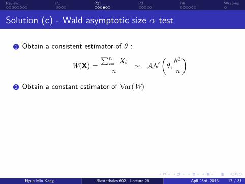
..........
.....
......
.....
.....
.....
......
.....
.....
.....
......
.....
.....
.....
......
.....
......
.....
.....
.
. . . . . . . .Review
. . . .P1
. . . . . .P2
. . . . .P3
. . . . . .P4
.Wrap-up
Solution (c) - Wald asymptotic size α test
..1 Obtain a consistent estimator of θ :
W(X) =
∑ni=1 Xin ∼ AN
(θ,
θ2
n
)..2 Obtain a constant estimator of Var(W)
1
n − 1
n∑i=1
(Xi − X)2P→ Var(X) =
1
θ2(CLT)
n − 1∑ni=1(Xi − X)2
P→ θ2 (Continuous Map Theorem).
S2 =n∑n
i=1(Xi − X)2P→ θ2 (Slutsky’s Theorem).
Hyun Min Kang Biostatistics 602 - Lecture 26 Apil 23rd, 2013 17 / 31
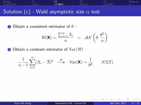
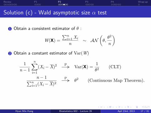
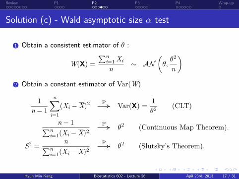

..........
.....
......
.....
.....
.....
......
.....
.....
.....
......
.....
.....
.....
......
.....
......
.....
.....
.
. . . . . . . .Review
. . . .P1
. . . . . .P2
. . . . .P3
. . . . . .P4
.Wrap-up
Solution (c) - Wald Asymptotic size α test (cont’d)
..3 Construct a two-sided asymptotic size α Wald test, whose rejectionregion is
|Z(X)| =
∣∣∣∣W(X)− θ0S/
√n
∣∣∣∣=
∣∣∣∣∣∣n∑n
i=1 Xi− θ0
1√∑ni=1(Xi−X)2
∣∣∣∣∣∣=
∣∣∣∣ 1X − θ0
∣∣∣∣√√√√ n∑
i=1
(Xi − X)2 ≥ zα/2
Hyun Min Kang Biostatistics 602 - Lecture 26 Apil 23rd, 2013 18 / 31
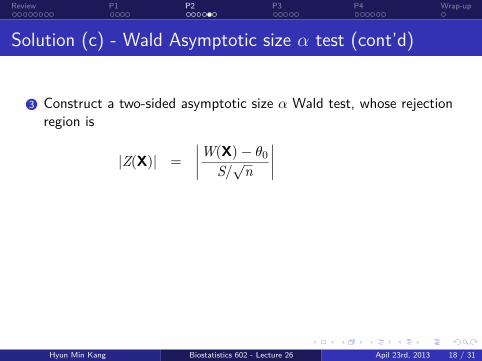
..........
.....
......
.....
.....
.....
......
.....
.....
.....
......
.....
.....
.....
......
.....
......
.....
.....
.
. . . . . . . .Review
. . . .P1
. . . . . .P2
. . . . .P3
. . . . . .P4
.Wrap-up
Solution (c) - Wald Asymptotic size α test (cont’d)
..3 Construct a two-sided asymptotic size α Wald test, whose rejectionregion is
|Z(X)| =
∣∣∣∣W(X)− θ0S/
√n
∣∣∣∣
=
∣∣∣∣∣∣n∑n
i=1 Xi− θ0
1√∑ni=1(Xi−X)2
∣∣∣∣∣∣=
∣∣∣∣ 1X − θ0
∣∣∣∣√√√√ n∑
i=1
(Xi − X)2 ≥ zα/2
Hyun Min Kang Biostatistics 602 - Lecture 26 Apil 23rd, 2013 18 / 31
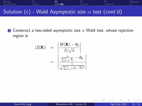
..........
.....
......
.....
.....
.....
......
.....
.....
.....
......
.....
.....
.....
......
.....
......
.....
.....
.
. . . . . . . .Review
. . . .P1
. . . . . .P2
. . . . .P3
. . . . . .P4
.Wrap-up
Solution (c) - Wald Asymptotic size α test (cont’d)
..3 Construct a two-sided asymptotic size α Wald test, whose rejectionregion is
|Z(X)| =
∣∣∣∣W(X)− θ0S/
√n
∣∣∣∣=
∣∣∣∣∣∣n∑n
i=1 Xi− θ0
1√∑ni=1(Xi−X)2
∣∣∣∣∣∣
=
∣∣∣∣ 1X − θ0
∣∣∣∣√√√√ n∑
i=1
(Xi − X)2 ≥ zα/2
Hyun Min Kang Biostatistics 602 - Lecture 26 Apil 23rd, 2013 18 / 31

..........
.....
......
.....
.....
.....
......
.....
.....
.....
......
.....
.....
.....
......
.....
......
.....
.....
.
. . . . . . . .Review
. . . .P1
. . . . . .P2
. . . . .P3
. . . . . .P4
.Wrap-up
Solution (c) - Wald Asymptotic size α test (cont’d)
..3 Construct a two-sided asymptotic size α Wald test, whose rejectionregion is
|Z(X)| =
∣∣∣∣W(X)− θ0S/
√n
∣∣∣∣=
∣∣∣∣∣∣n∑n
i=1 Xi− θ0
1√∑ni=1(Xi−X)2
∣∣∣∣∣∣=
∣∣∣∣ 1X − θ0
∣∣∣∣√√√√ n∑
i=1
(Xi − X)2 ≥ zα/2
Hyun Min Kang Biostatistics 602 - Lecture 26 Apil 23rd, 2013 18 / 31

..........
.....
......
.....
.....
.....
......
.....
.....
.....
......
.....
.....
.....
......
.....
......
.....
.....
.
. . . . . . . .Review
. . . .P1
. . . . . .P2
. . . . .P3
. . . . . .P4
.Wrap-up
Solution (d) - Asymptotic 1− α confidence intervalThe acceptance region is
A =
x :
∣∣∣∣1x − θ0
∣∣∣∣√√√√ n∑
i=1
(xi − x)2 ≤ zα/2
By inverting the acceptance region, the confidence interval is
C(X) =
θ :
∣∣∣∣ 1X − θ
∣∣∣∣√√√√ n∑
i=1
(Xi − X)2 ≤ zα/2
which is equivalent to
C(X) =
θ ∈
1
X−
zα/2√∑ni=1(Xi − X)2
,1
X+
zα/2√∑ni=1(Xi − X)2
Hyun Min Kang Biostatistics 602 - Lecture 26 Apil 23rd, 2013 19 / 31

..........
.....
......
.....
.....
.....
......
.....
.....
.....
......
.....
.....
.....
......
.....
......
.....
.....
.
. . . . . . . .Review
. . . .P1
. . . . . .P2
. . . . .P3
. . . . . .P4
.Wrap-up
Practice Problem 3
.Problem..
......
The independent random variables X1, · · · ,Xn have the following pdf
f(x|θ, β) =βxβ−1
θβ0 < x < θ, β > 0
..1 Find the MLEs of β and θ
..2 When β is a known constant β0, construct a LRT testing H0 : θ ≥ θ0vs. H1 : θ < θ0.
..3 When β is a known constant β0, find the upper confidence limit for θwith confidence coefficient 1− α.
Hyun Min Kang Biostatistics 602 - Lecture 26 Apil 23rd, 2013 20 / 31
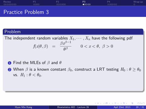
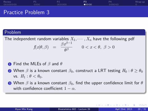

..........
.....
......
.....
.....
.....
......
.....
.....
.....
......
.....
.....
.....
......
.....
......
.....
.....
.
. . . . . . . .Review
. . . .P1
. . . . . .P2
. . . . .P3
. . . . . .P4
.Wrap-up
(a) - MLE
L(θ, β|x) =βn (
∏ni=1 xi)
β−1
θnβ I(x(n) ≤ θ)
Because L is a decreasing function of θ and positive only when θ ≥ x(n)θ = x(n)
l(θ, β|x) = n logβ + (β − 1)∑
log xi − nβ log θ∂l∂β
=nβ+∑
log xi − n log θ = 0
β =n
n log θ −∑
log xi
=n
nx(n) −∑
log xi
Hyun Min Kang Biostatistics 602 - Lecture 26 Apil 23rd, 2013 21 / 31

..........
.....
......
.....
.....
.....
......
.....
.....
.....
......
.....
.....
.....
......
.....
......
.....
.....
.
. . . . . . . .Review
. . . .P1
. . . . . .P2
. . . . .P3
. . . . . .P4
.Wrap-up
(a) - MLE
L(θ, β|x) =βn (
∏ni=1 xi)
β−1
θnβ I(x(n) ≤ θ)
Because L is a decreasing function of θ and positive only when θ ≥ x(n)
θ = x(n)l(θ, β|x) = n logβ + (β − 1)
∑log xi − nβ log θ
∂l∂β
=nβ+∑
log xi − n log θ = 0
β =n
n log θ −∑
log xi
=n
nx(n) −∑
log xi
Hyun Min Kang Biostatistics 602 - Lecture 26 Apil 23rd, 2013 21 / 31

..........
.....
......
.....
.....
.....
......
.....
.....
.....
......
.....
.....
.....
......
.....
......
.....
.....
.
. . . . . . . .Review
. . . .P1
. . . . . .P2
. . . . .P3
. . . . . .P4
.Wrap-up
(a) - MLE
L(θ, β|x) =βn (
∏ni=1 xi)
β−1
θnβ I(x(n) ≤ θ)
Because L is a decreasing function of θ and positive only when θ ≥ x(n)θ = x(n)
l(θ, β|x) = n logβ + (β − 1)∑
log xi − nβ log θ∂l∂β
=nβ+∑
log xi − n log θ = 0
β =n
n log θ −∑
log xi
=n
nx(n) −∑
log xi
Hyun Min Kang Biostatistics 602 - Lecture 26 Apil 23rd, 2013 21 / 31

..........
.....
......
.....
.....
.....
......
.....
.....
.....
......
.....
.....
.....
......
.....
......
.....
.....
.
. . . . . . . .Review
. . . .P1
. . . . . .P2
. . . . .P3
. . . . . .P4
.Wrap-up
(a) - MLE
L(θ, β|x) =βn (
∏ni=1 xi)
β−1
θnβ I(x(n) ≤ θ)
Because L is a decreasing function of θ and positive only when θ ≥ x(n)θ = x(n)
l(θ, β|x) = n logβ + (β − 1)∑
log xi − nβ log θ
∂l∂β
=nβ+∑
log xi − n log θ = 0
β =n
n log θ −∑
log xi
=n
nx(n) −∑
log xi
Hyun Min Kang Biostatistics 602 - Lecture 26 Apil 23rd, 2013 21 / 31
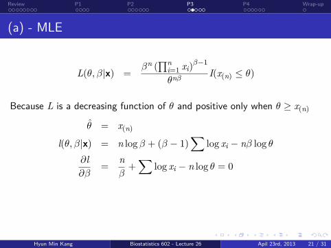
..........
.....
......
.....
.....
.....
......
.....
.....
.....
......
.....
.....
.....
......
.....
......
.....
.....
.
. . . . . . . .Review
. . . .P1
. . . . . .P2
. . . . .P3
. . . . . .P4
.Wrap-up
(a) - MLE
L(θ, β|x) =βn (
∏ni=1 xi)
β−1
θnβ I(x(n) ≤ θ)
Because L is a decreasing function of θ and positive only when θ ≥ x(n)θ = x(n)
l(θ, β|x) = n logβ + (β − 1)∑
log xi − nβ log θ∂l∂β
=nβ+∑
log xi − n log θ = 0
β =n
n log θ −∑
log xi
=n
nx(n) −∑
log xi
Hyun Min Kang Biostatistics 602 - Lecture 26 Apil 23rd, 2013 21 / 31
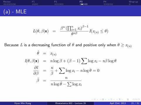
..........
.....
......
.....
.....
.....
......
.....
.....
.....
......
.....
.....
.....
......
.....
......
.....
.....
.
. . . . . . . .Review
. . . .P1
. . . . . .P2
. . . . .P3
. . . . . .P4
.Wrap-up
(a) - MLE
L(θ, β|x) =βn (
∏ni=1 xi)
β−1
θnβ I(x(n) ≤ θ)
Because L is a decreasing function of θ and positive only when θ ≥ x(n)θ = x(n)
l(θ, β|x) = n logβ + (β − 1)∑
log xi − nβ log θ∂l∂β
=nβ+∑
log xi − n log θ = 0
β =n
n log θ −∑
log xi
=n
nx(n) −∑
log xi
Hyun Min Kang Biostatistics 602 - Lecture 26 Apil 23rd, 2013 21 / 31
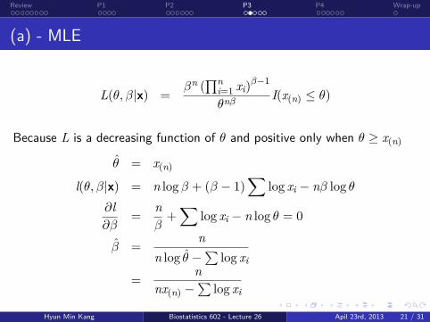
..........
.....
......
.....
.....
.....
......
.....
.....
.....
......
.....
.....
.....
......
.....
......
.....
.....
.
. . . . . . . .Review
. . . .P1
. . . . . .P2
. . . . .P3
. . . . . .P4
.Wrap-up
(a) - MLE
L(θ, β|x) =βn (
∏ni=1 xi)
β−1
θnβ I(x(n) ≤ θ)
Because L is a decreasing function of θ and positive only when θ ≥ x(n)θ = x(n)
l(θ, β|x) = n logβ + (β − 1)∑
log xi − nβ log θ∂l∂β
=nβ+∑
log xi − n log θ = 0
β =n
n log θ −∑
log xi
=n
nx(n) −∑
log xi
Hyun Min Kang Biostatistics 602 - Lecture 26 Apil 23rd, 2013 21 / 31
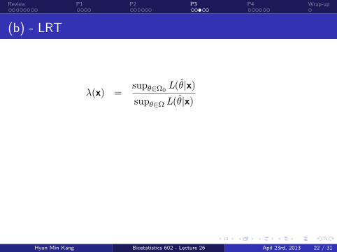
..........
.....
......
.....
.....
.....
......
.....
.....
.....
......
.....
.....
.....
......
.....
......
.....
.....
.
. . . . . . . .Review
. . . .P1
. . . . . .P2
. . . . .P3
. . . . . .P4
.Wrap-up
(b) - LRT
λ(x) =supθ∈Ω0
L(θ|x)supθ∈Ω L(θ|x)
=
1 θ0 < x(n)L(θ0|x)
L(x(n)|x) θ0 ≥ x(n)
=
1 θ0 < x(n)(x(n))
nβ0
θnβ00
θ0 ≥ x(n)≤ c
x(n)θ0
≤ c∗
Hyun Min Kang Biostatistics 602 - Lecture 26 Apil 23rd, 2013 22 / 31
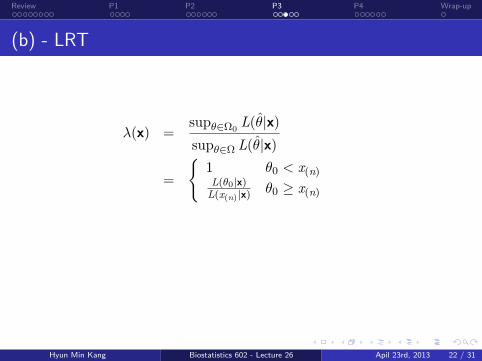
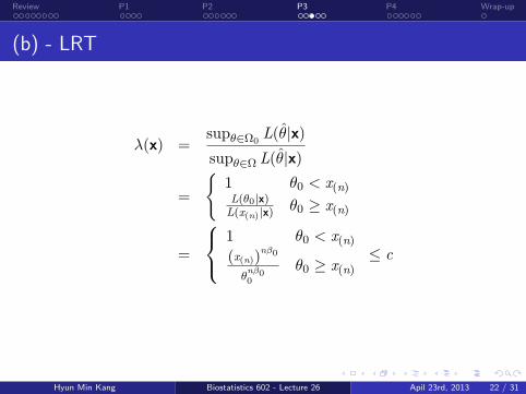
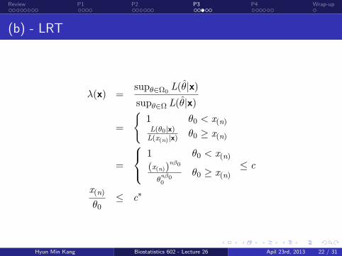
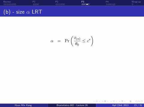
..........
.....
......
.....
.....
.....
......
.....
.....
.....
......
.....
.....
.....
......
.....
......
.....
.....
.
. . . . . . . .Review
. . . .P1
. . . . . .P2
. . . . .P3
. . . . . .P4
.Wrap-up
(b) - size α LRT
α = Pr(x(n)
θ0≤ c∗
)
= (c∗)nβ0
c∗ = α1
nβ0
Therefore, the rejection region for size α LRT is is
R =
x : x(n) ≤ θ0α1
nβ0
Hyun Min Kang Biostatistics 602 - Lecture 26 Apil 23rd, 2013 23 / 31
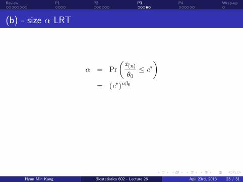
..........
.....
......
.....
.....
.....
......
.....
.....
.....
......
.....
.....
.....
......
.....
......
.....
.....
.
. . . . . . . .Review
. . . .P1
. . . . . .P2
. . . . .P3
. . . . . .P4
.Wrap-up
(b) - size α LRT
α = Pr(x(n)
θ0≤ c∗
)= (c∗)nβ0
c∗ = α1
nβ0
Therefore, the rejection region for size α LRT is is
R =
x : x(n) ≤ θ0α1
nβ0
Hyun Min Kang Biostatistics 602 - Lecture 26 Apil 23rd, 2013 23 / 31
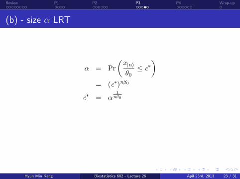
..........
.....
......
.....
.....
.....
......
.....
.....
.....
......
.....
.....
.....
......
.....
......
.....
.....
.
. . . . . . . .Review
. . . .P1
. . . . . .P2
. . . . .P3
. . . . . .P4
.Wrap-up
(b) - size α LRT
α = Pr(x(n)
θ0≤ c∗
)= (c∗)nβ0
c∗ = α1
nβ0
Therefore, the rejection region for size α LRT is is
R =
x : x(n) ≤ θ0α1
nβ0
Hyun Min Kang Biostatistics 602 - Lecture 26 Apil 23rd, 2013 23 / 31
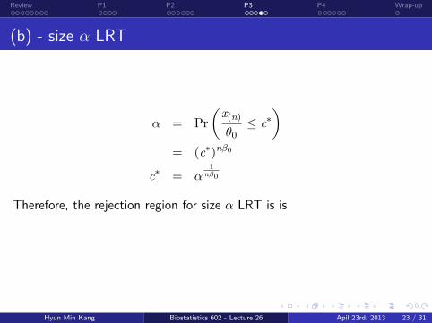
..........
.....
......
.....
.....
.....
......
.....
.....
.....
......
.....
.....
.....
......
.....
......
.....
.....
.
. . . . . . . .Review
. . . .P1
. . . . . .P2
. . . . .P3
. . . . . .P4
.Wrap-up
(b) - size α LRT
α = Pr(x(n)
θ0≤ c∗
)= (c∗)nβ0
c∗ = α1
nβ0
Therefore, the rejection region for size α LRT is is
R =
x : x(n) ≤ θ0α1
nβ0
Hyun Min Kang Biostatistics 602 - Lecture 26 Apil 23rd, 2013 23 / 31
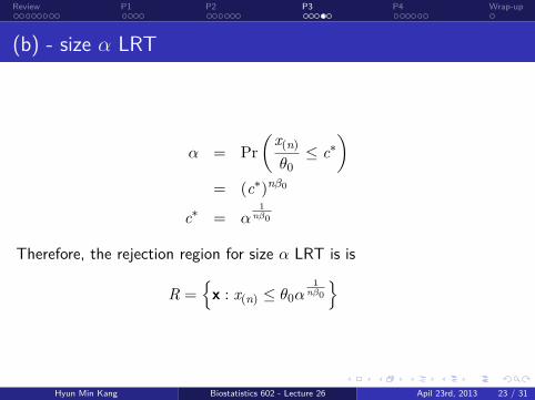
..........
.....
......
.....
.....
.....
......
.....
.....
.....
......
.....
.....
.....
......
.....
......
.....
.....
.
. . . . . . . .Review
. . . .P1
. . . . . .P2
. . . . .P3
. . . . . .P4
.Wrap-up
(b) - size α LRT
α = Pr(x(n)
θ0≤ c∗
)= (c∗)nβ0
c∗ = α1
nβ0
Therefore, the rejection region for size α LRT is is
R =
x : x(n) ≤ θ0α1
nβ0
Hyun Min Kang Biostatistics 602 - Lecture 26 Apil 23rd, 2013 23 / 31

..........
.....
......
.....
.....
.....
......
.....
.....
.....
......
.....
.....
.....
......
.....
......
.....
.....
.
. . . . . . . .Review
. . . .P1
. . . . . .P2
. . . . .P3
. . . . . .P4
.Wrap-up
(c) - Upper 1− α confidence limit
The acceptance region of size α LRT is
A(θ0) =
x : x(n) > θ0α1
nβ0
By inserting the acceptance region, the 1− α confidence interval becomes
C(X) =θ : X(n) > θα
1nβ0
=
θ : θ < X(n)α
− 1nβ0
Therefore, the upper 1− α confidence limit is X(n)α− 1
nβ0 .
Hyun Min Kang Biostatistics 602 - Lecture 26 Apil 23rd, 2013 24 / 31
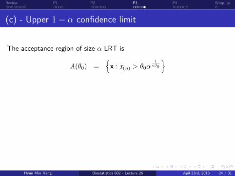
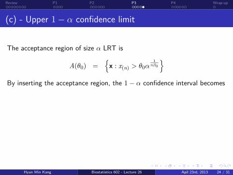
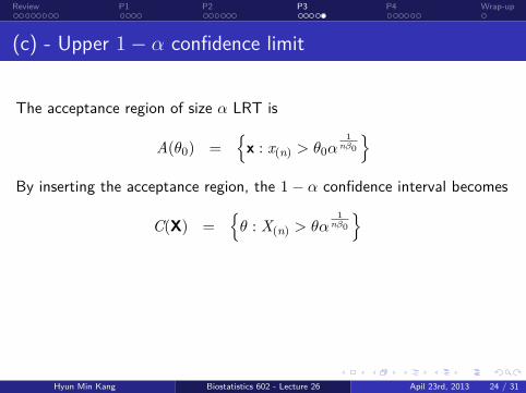
..........
.....
......
.....
.....
.....
......
.....
.....
.....
......
.....
.....
.....
......
.....
......
.....
.....
.
. . . . . . . .Review
. . . .P1
. . . . . .P2
. . . . .P3
. . . . . .P4
.Wrap-up
(c) - Upper 1− α confidence limit
The acceptance region of size α LRT is
A(θ0) =
x : x(n) > θ0α1
nβ0
By inserting the acceptance region, the 1− α confidence interval becomes
C(X) =θ : X(n) > θα
1nβ0
=θ : θ < X(n)α
− 1nβ0
Therefore, the upper 1− α confidence limit is X(n)α− 1
nβ0 .
Hyun Min Kang Biostatistics 602 - Lecture 26 Apil 23rd, 2013 24 / 31
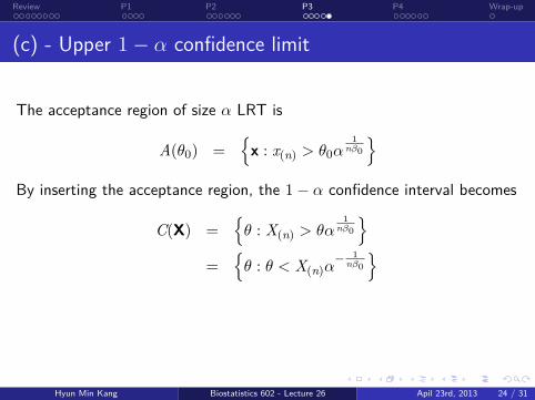
..........
.....
......
.....
.....
.....
......
.....
.....
.....
......
.....
.....
.....
......
.....
......
.....
.....
.
. . . . . . . .Review
. . . .P1
. . . . . .P2
. . . . .P3
. . . . . .P4
.Wrap-up
(c) - Upper 1− α confidence limit
The acceptance region of size α LRT is
A(θ0) =
x : x(n) > θ0α1
nβ0
By inserting the acceptance region, the 1− α confidence interval becomes
C(X) =θ : X(n) > θα
1nβ0
=
θ : θ < X(n)α
− 1nβ0
Therefore, the upper 1− α confidence limit is X(n)α− 1
nβ0 .
Hyun Min Kang Biostatistics 602 - Lecture 26 Apil 23rd, 2013 24 / 31
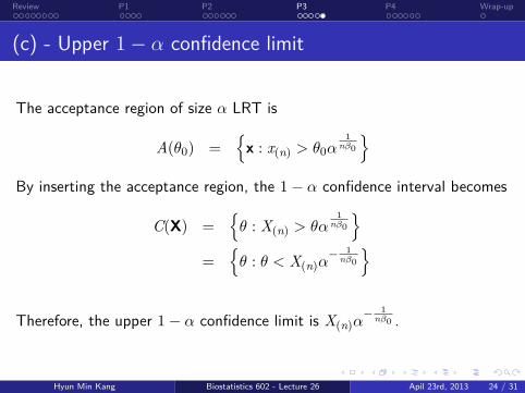
..........
.....
......
.....
.....
.....
......
.....
.....
.....
......
.....
.....
.....
......
.....
......
.....
.....
.
. . . . . . . .Review
. . . .P1
. . . . . .P2
. . . . .P3
. . . . . .P4
.Wrap-up
(c) - Upper 1− α confidence limit
The acceptance region of size α LRT is
A(θ0) =
x : x(n) > θ0α1
nβ0
By inserting the acceptance region, the 1− α confidence interval becomes
C(X) =θ : X(n) > θα
1nβ0
=
θ : θ < X(n)α
− 1nβ0
Therefore, the upper 1− α confidence limit is X(n)α− 1
nβ0 .
Hyun Min Kang Biostatistics 602 - Lecture 26 Apil 23rd, 2013 24 / 31

..........
.....
......
.....
.....
.....
......
.....
.....
.....
......
.....
.....
.....
......
.....
......
.....
.....
.
. . . . . . . .Review
. . . .P1
. . . . . .P2
. . . . .P3
. . . . . .P4
.Wrap-up
Practice Problem 4
.Problem..
......
A random sample X1, · · · ,Xn is drawn from a population N (θ, θ) whereθ > 0.
(a) Find the θ, the MLE of θ(b) Find the asymptotic distribution of θ.(c) Compute ARE(θ,X). Determine whether θ is asymptotically more
efficient than X or not.You may use the following fact: Var(X2) = 4θ3 + 2θ2.
Hyun Min Kang Biostatistics 602 - Lecture 26 Apil 23rd, 2013 25 / 31
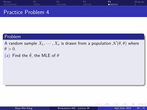
..........
.....
......
.....
.....
.....
......
.....
.....
.....
......
.....
.....
.....
......
.....
......
.....
.....
.
. . . . . . . .Review
. . . .P1
. . . . . .P2
. . . . .P3
. . . . . .P4
.Wrap-up
Practice Problem 4
.Problem..
......
A random sample X1, · · · ,Xn is drawn from a population N (θ, θ) whereθ > 0.(a) Find the θ, the MLE of θ
(b) Find the asymptotic distribution of θ.(c) Compute ARE(θ,X). Determine whether θ is asymptotically more
efficient than X or not.You may use the following fact: Var(X2) = 4θ3 + 2θ2.
Hyun Min Kang Biostatistics 602 - Lecture 26 Apil 23rd, 2013 25 / 31
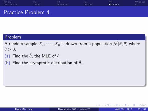
..........
.....
......
.....
.....
.....
......
.....
.....
.....
......
.....
.....
.....
......
.....
......
.....
.....
.
. . . . . . . .Review
. . . .P1
. . . . . .P2
. . . . .P3
. . . . . .P4
.Wrap-up
Practice Problem 4
.Problem..
......
A random sample X1, · · · ,Xn is drawn from a population N (θ, θ) whereθ > 0.(a) Find the θ, the MLE of θ(b) Find the asymptotic distribution of θ.
(c) Compute ARE(θ,X). Determine whether θ is asymptotically moreefficient than X or not.
You may use the following fact: Var(X2) = 4θ3 + 2θ2.
Hyun Min Kang Biostatistics 602 - Lecture 26 Apil 23rd, 2013 25 / 31
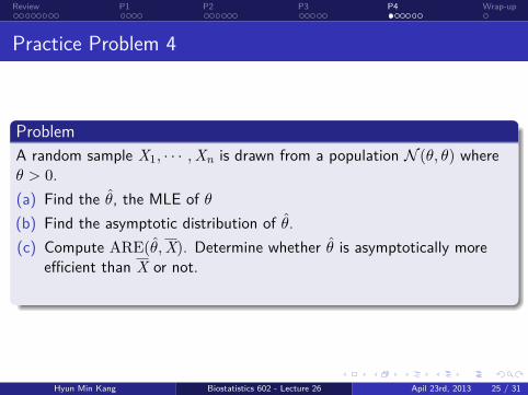
..........
.....
......
.....
.....
.....
......
.....
.....
.....
......
.....
.....
.....
......
.....
......
.....
.....
.
. . . . . . . .Review
. . . .P1
. . . . . .P2
. . . . .P3
. . . . . .P4
.Wrap-up
Practice Problem 4
.Problem..
......
A random sample X1, · · · ,Xn is drawn from a population N (θ, θ) whereθ > 0.(a) Find the θ, the MLE of θ(b) Find the asymptotic distribution of θ.(c) Compute ARE(θ,X). Determine whether θ is asymptotically more
efficient than X or not.
You may use the following fact: Var(X2) = 4θ3 + 2θ2.
Hyun Min Kang Biostatistics 602 - Lecture 26 Apil 23rd, 2013 25 / 31
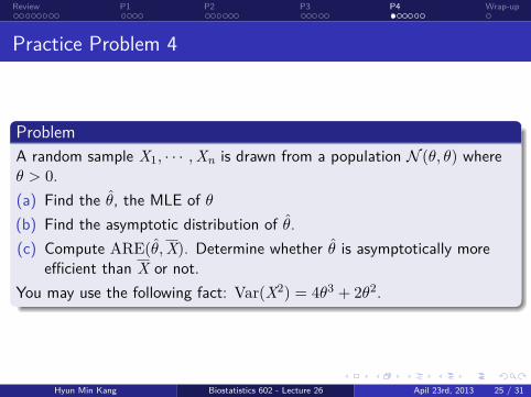
..........
.....
......
.....
.....
.....
......
.....
.....
.....
......
.....
.....
.....
......
.....
......
.....
.....
.
. . . . . . . .Review
. . . .P1
. . . . . .P2
. . . . .P3
. . . . . .P4
.Wrap-up
Practice Problem 4
.Problem..
......
A random sample X1, · · · ,Xn is drawn from a population N (θ, θ) whereθ > 0.(a) Find the θ, the MLE of θ(b) Find the asymptotic distribution of θ.(c) Compute ARE(θ,X). Determine whether θ is asymptotically more
efficient than X or not.You may use the following fact: Var(X2) = 4θ3 + 2θ2.
Hyun Min Kang Biostatistics 602 - Lecture 26 Apil 23rd, 2013 25 / 31

..........
.....
......
.....
.....
.....
......
.....
.....
.....
......
.....
.....
.....
......
.....
......
.....
.....
.
. . . . . . . .Review
. . . .P1
. . . . . .P2
. . . . .P3
. . . . . .P4
.Wrap-up
(a) - MLE of θ
L(θ|x) = (2πθ)n/2 exp[−∑n
i=1(xi − θ)2
2θ
]
l(θ|x) =n2
log(2π) + n2
log θ −∑n
i=1(xi − θ)2
2θ
=n2
log(2π) + n2
log θ −∑
x2i2θ
+∑
xi −nθ2
l′(θ|x) =n2θ
+
∑x2i
2θ2− n
2=
nθ −∑
x2i − nθ22θ2
= 0
nθ2 + nθ −∑
x2i = 0
θ =−1 +
√1 + 4
∑x2i /n
21
n∑
x2i = θ2 + θ
Hyun Min Kang Biostatistics 602 - Lecture 26 Apil 23rd, 2013 26 / 31

..........
.....
......
.....
.....
.....
......
.....
.....
.....
......
.....
.....
.....
......
.....
......
.....
.....
.
. . . . . . . .Review
. . . .P1
. . . . . .P2
. . . . .P3
. . . . . .P4
.Wrap-up
(a) - MLE of θ
L(θ|x) = (2πθ)n/2 exp[−∑n
i=1(xi − θ)2
2θ
]l(θ|x) =
n2
log(2π) + n2
log θ −∑n
i=1(xi − θ)2
2θ
=n2
log(2π) + n2
log θ −∑
x2i2θ
+∑
xi −nθ2
l′(θ|x) =n2θ
+
∑x2i
2θ2− n
2=
nθ −∑
x2i − nθ22θ2
= 0
nθ2 + nθ −∑
x2i = 0
θ =−1 +
√1 + 4
∑x2i /n
21
n∑
x2i = θ2 + θ
Hyun Min Kang Biostatistics 602 - Lecture 26 Apil 23rd, 2013 26 / 31
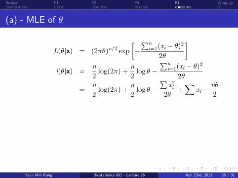
..........
.....
......
.....
.....
.....
......
.....
.....
.....
......
.....
.....
.....
......
.....
......
.....
.....
.
. . . . . . . .Review
. . . .P1
. . . . . .P2
. . . . .P3
. . . . . .P4
.Wrap-up
(a) - MLE of θ
L(θ|x) = (2πθ)n/2 exp[−∑n
i=1(xi − θ)2
2θ
]l(θ|x) =
n2
log(2π) + n2
log θ −∑n
i=1(xi − θ)2
2θ
=n2
log(2π) + n2
log θ −∑
x2i2θ
+∑
xi −nθ2
l′(θ|x) =n2θ
+
∑x2i
2θ2− n
2=
nθ −∑
x2i − nθ22θ2
= 0
nθ2 + nθ −∑
x2i = 0
θ =−1 +
√1 + 4
∑x2i /n
21
n∑
x2i = θ2 + θ
Hyun Min Kang Biostatistics 602 - Lecture 26 Apil 23rd, 2013 26 / 31
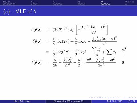
..........
.....
......
.....
.....
.....
......
.....
.....
.....
......
.....
.....
.....
......
.....
......
.....
.....
.
. . . . . . . .Review
. . . .P1
. . . . . .P2
. . . . .P3
. . . . . .P4
.Wrap-up
(a) - MLE of θ
L(θ|x) = (2πθ)n/2 exp[−∑n
i=1(xi − θ)2
2θ
]l(θ|x) =
n2
log(2π) + n2
log θ −∑n
i=1(xi − θ)2
2θ
=n2
log(2π) + n2
log θ −∑
x2i2θ
+∑
xi −nθ2
l′(θ|x) =n2θ
+
∑x2i
2θ2− n
2=
nθ −∑
x2i − nθ22θ2
= 0
nθ2 + nθ −∑
x2i = 0
θ =−1 +
√1 + 4
∑x2i /n
21
n∑
x2i = θ2 + θ
Hyun Min Kang Biostatistics 602 - Lecture 26 Apil 23rd, 2013 26 / 31
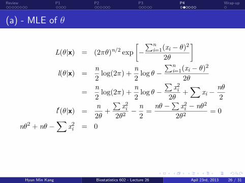
..........
.....
......
.....
.....
.....
......
.....
.....
.....
......
.....
.....
.....
......
.....
......
.....
.....
.
. . . . . . . .Review
. . . .P1
. . . . . .P2
. . . . .P3
. . . . . .P4
.Wrap-up
(a) - MLE of θ
L(θ|x) = (2πθ)n/2 exp[−∑n
i=1(xi − θ)2
2θ
]l(θ|x) =
n2
log(2π) + n2
log θ −∑n
i=1(xi − θ)2
2θ
=n2
log(2π) + n2
log θ −∑
x2i2θ
+∑
xi −nθ2
l′(θ|x) =n2θ
+
∑x2i
2θ2− n
2=
nθ −∑
x2i − nθ22θ2
= 0
nθ2 + nθ −∑
x2i = 0
θ =−1 +
√1 + 4
∑x2i /n
2
1
n∑
x2i = θ2 + θ
Hyun Min Kang Biostatistics 602 - Lecture 26 Apil 23rd, 2013 26 / 31

..........
.....
......
.....
.....
.....
......
.....
.....
.....
......
.....
.....
.....
......
.....
......
.....
.....
.
. . . . . . . .Review
. . . .P1
. . . . . .P2
. . . . .P3
. . . . . .P4
.Wrap-up
(a) - MLE of θ
L(θ|x) = (2πθ)n/2 exp[−∑n
i=1(xi − θ)2
2θ
]l(θ|x) =
n2
log(2π) + n2
log θ −∑n
i=1(xi − θ)2
2θ
=n2
log(2π) + n2
log θ −∑
x2i2θ
+∑
xi −nθ2
l′(θ|x) =n2θ
+
∑x2i
2θ2− n
2=
nθ −∑
x2i − nθ22θ2
= 0
nθ2 + nθ −∑
x2i = 0
θ =−1 +
√1 + 4
∑x2i /n
21
n∑
x2i = θ2 + θ
Hyun Min Kang Biostatistics 602 - Lecture 26 Apil 23rd, 2013 26 / 31
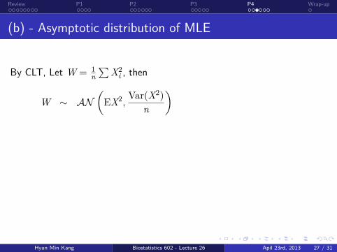
..........
.....
......
.....
.....
.....
......
.....
.....
.....
......
.....
.....
.....
......
.....
......
.....
.....
.
. . . . . . . .Review
. . . .P1
. . . . . .P2
. . . . .P3
. . . . . .P4
.Wrap-up
(b) - Asymptotic distribution of MLE
By CLT, Let W = 1n∑
X2i , then
W ∼ AN(
EX2,Var(X2)
n
)
= AN(θ + θ2,
4θ3 + 2θ2
n
)The asymptotic distribution of MLE θ
θ ∼ AN(θ,
σ2(θ)
n
)for some function σ2(θ) and we would like to find σ2(θ) using theasymptotic distribution of W.
Hyun Min Kang Biostatistics 602 - Lecture 26 Apil 23rd, 2013 27 / 31
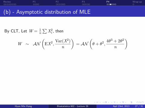
..........
.....
......
.....
.....
.....
......
.....
.....
.....
......
.....
.....
.....
......
.....
......
.....
.....
.
. . . . . . . .Review
. . . .P1
. . . . . .P2
. . . . .P3
. . . . . .P4
.Wrap-up
(b) - Asymptotic distribution of MLE
By CLT, Let W = 1n∑
X2i , then
W ∼ AN(
EX2,Var(X2)
n
)= AN
(θ + θ2,
4θ3 + 2θ2
n
)
The asymptotic distribution of MLE θ
θ ∼ AN(θ,
σ2(θ)
n
)for some function σ2(θ) and we would like to find σ2(θ) using theasymptotic distribution of W.
Hyun Min Kang Biostatistics 602 - Lecture 26 Apil 23rd, 2013 27 / 31
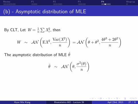
..........
.....
......
.....
.....
.....
......
.....
.....
.....
......
.....
.....
.....
......
.....
......
.....
.....
.
. . . . . . . .Review
. . . .P1
. . . . . .P2
. . . . .P3
. . . . . .P4
.Wrap-up
(b) - Asymptotic distribution of MLE
By CLT, Let W = 1n∑
X2i , then
W ∼ AN(
EX2,Var(X2)
n
)= AN
(θ + θ2,
4θ3 + 2θ2
n
)The asymptotic distribution of MLE θ
θ ∼ AN(θ,
σ2(θ)
n
)
for some function σ2(θ) and we would like to find σ2(θ) using theasymptotic distribution of W.
Hyun Min Kang Biostatistics 602 - Lecture 26 Apil 23rd, 2013 27 / 31
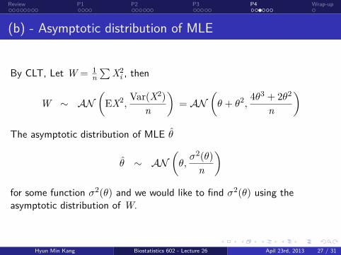
..........
.....
......
.....
.....
.....
......
.....
.....
.....
......
.....
.....
.....
......
.....
......
.....
.....
.
. . . . . . . .Review
. . . .P1
. . . . . .P2
. . . . .P3
. . . . . .P4
.Wrap-up
(b) - Asymptotic distribution of MLE
By CLT, Let W = 1n∑
X2i , then
W ∼ AN(
EX2,Var(X2)
n
)= AN
(θ + θ2,
4θ3 + 2θ2
n
)The asymptotic distribution of MLE θ
θ ∼ AN(θ,
σ2(θ)
n
)for some function σ2(θ) and we would like to find σ2(θ) using theasymptotic distribution of W.
Hyun Min Kang Biostatistics 602 - Lecture 26 Apil 23rd, 2013 27 / 31

..........
.....
......
.....
.....
.....
......
.....
.....
.....
......
.....
.....
.....
......
.....
......
.....
.....
.
. . . . . . . .Review
. . . .P1
. . . . . .P2
. . . . .P3
. . . . . .P4
.Wrap-up
(b) - Asymptotic distribution of MLE (cont’d)
Let g(y) = y2 + y, then g′(y) = (2y + 1) and g(θ) = W. Then by theDelta Method, the asymptotic distribution of W can be written as
W = g(θ) ∼ AN(
g(θ), g′(θ)σ2(θ)
n
)= AN
(θ2 + θ,
(2θ + 1)2σ2(θ)
n
)= AN
(θ2 + θ,
4θ3 + 2θ2
n
)σ2(θ) =
4θ3 + 2θ2
(2θ + 1)2=
2θ2(2θ + 1)
(2θ + 1)2=
2θ2
2θ + 1
Hyun Min Kang Biostatistics 602 - Lecture 26 Apil 23rd, 2013 28 / 31
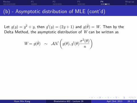
..........
.....
......
.....
.....
.....
......
.....
.....
.....
......
.....
.....
.....
......
.....
......
.....
.....
.
. . . . . . . .Review
. . . .P1
. . . . . .P2
. . . . .P3
. . . . . .P4
.Wrap-up
(b) - Asymptotic distribution of MLE (cont’d)
Let g(y) = y2 + y, then g′(y) = (2y + 1) and g(θ) = W. Then by theDelta Method, the asymptotic distribution of W can be written as
W = g(θ) ∼ AN(
g(θ), g′(θ)σ2(θ)
n
)
= AN(θ2 + θ,
(2θ + 1)2σ2(θ)
n
)= AN
(θ2 + θ,
4θ3 + 2θ2
n
)σ2(θ) =
4θ3 + 2θ2
(2θ + 1)2=
2θ2(2θ + 1)
(2θ + 1)2=
2θ2
2θ + 1
Hyun Min Kang Biostatistics 602 - Lecture 26 Apil 23rd, 2013 28 / 31
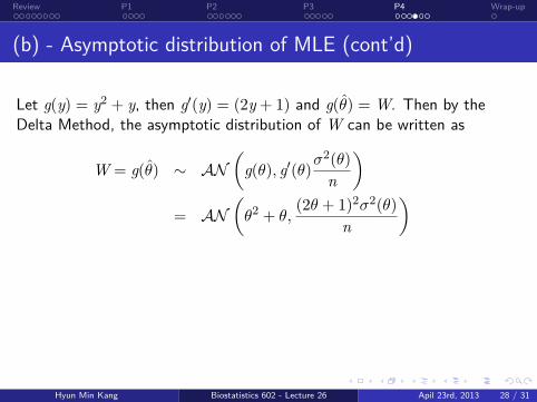
..........
.....
......
.....
.....
.....
......
.....
.....
.....
......
.....
.....
.....
......
.....
......
.....
.....
.
. . . . . . . .Review
. . . .P1
. . . . . .P2
. . . . .P3
. . . . . .P4
.Wrap-up
(b) - Asymptotic distribution of MLE (cont’d)
Let g(y) = y2 + y, then g′(y) = (2y + 1) and g(θ) = W. Then by theDelta Method, the asymptotic distribution of W can be written as
W = g(θ) ∼ AN(
g(θ), g′(θ)σ2(θ)
n
)= AN
(θ2 + θ,
(2θ + 1)2σ2(θ)
n
)
= AN(θ2 + θ,
4θ3 + 2θ2
n
)σ2(θ) =
4θ3 + 2θ2
(2θ + 1)2=
2θ2(2θ + 1)
(2θ + 1)2=
2θ2
2θ + 1
Hyun Min Kang Biostatistics 602 - Lecture 26 Apil 23rd, 2013 28 / 31
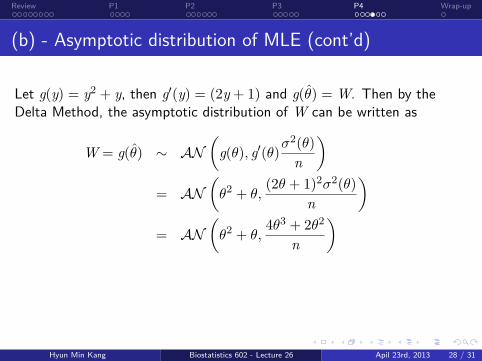
..........
.....
......
.....
.....
.....
......
.....
.....
.....
......
.....
.....
.....
......
.....
......
.....
.....
.
. . . . . . . .Review
. . . .P1
. . . . . .P2
. . . . .P3
. . . . . .P4
.Wrap-up
(b) - Asymptotic distribution of MLE (cont’d)
Let g(y) = y2 + y, then g′(y) = (2y + 1) and g(θ) = W. Then by theDelta Method, the asymptotic distribution of W can be written as
W = g(θ) ∼ AN(
g(θ), g′(θ)σ2(θ)
n
)= AN
(θ2 + θ,
(2θ + 1)2σ2(θ)
n
)= AN
(θ2 + θ,
4θ3 + 2θ2
n
)
σ2(θ) =4θ3 + 2θ2
(2θ + 1)2=
2θ2(2θ + 1)
(2θ + 1)2=
2θ2
2θ + 1
Hyun Min Kang Biostatistics 602 - Lecture 26 Apil 23rd, 2013 28 / 31
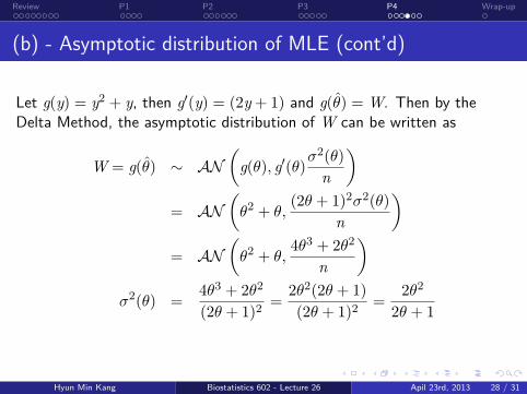
..........
.....
......
.....
.....
.....
......
.....
.....
.....
......
.....
.....
.....
......
.....
......
.....
.....
.
. . . . . . . .Review
. . . .P1
. . . . . .P2
. . . . .P3
. . . . . .P4
.Wrap-up
(b) - Asymptotic distribution of MLE (cont’d)
Let g(y) = y2 + y, then g′(y) = (2y + 1) and g(θ) = W. Then by theDelta Method, the asymptotic distribution of W can be written as
W = g(θ) ∼ AN(
g(θ), g′(θ)σ2(θ)
n
)= AN
(θ2 + θ,
(2θ + 1)2σ2(θ)
n
)= AN
(θ2 + θ,
4θ3 + 2θ2
n
)σ2(θ) =
4θ3 + 2θ2
(2θ + 1)2=
2θ2(2θ + 1)
(2θ + 1)2=
2θ2
2θ + 1
Hyun Min Kang Biostatistics 602 - Lecture 26 Apil 23rd, 2013 28 / 31
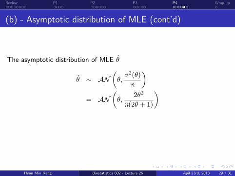
..........
.....
......
.....
.....
.....
......
.....
.....
.....
......
.....
.....
.....
......
.....
......
.....
.....
.
. . . . . . . .Review
. . . .P1
. . . . . .P2
. . . . .P3
. . . . . .P4
.Wrap-up
(b) - Asymptotic distribution of MLE (cont’d)
The asymptotic distribution of MLE θ
θ ∼ AN(θ,
σ2(θ)
n
)= AN
(θ,
2θ2
n(2θ + 1)
)
Note that you cannot use CR-bound for the asymptotic variance of MLEbecause the regularity condition does not hold (open set criteria).
Hyun Min Kang Biostatistics 602 - Lecture 26 Apil 23rd, 2013 29 / 31
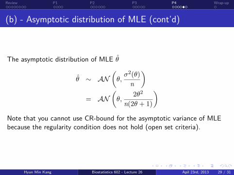
..........
.....
......
.....
.....
.....
......
.....
.....
.....
......
.....
.....
.....
......
.....
......
.....
.....
.
. . . . . . . .Review
. . . .P1
. . . . . .P2
. . . . .P3
. . . . . .P4
.Wrap-up
(b) - Asymptotic distribution of MLE (cont’d)
The asymptotic distribution of MLE θ
θ ∼ AN(θ,
σ2(θ)
n
)= AN
(θ,
2θ2
n(2θ + 1)
)Note that you cannot use CR-bound for the asymptotic variance of MLEbecause the regularity condition does not hold (open set criteria).
Hyun Min Kang Biostatistics 602 - Lecture 26 Apil 23rd, 2013 29 / 31

..........
.....
......
.....
.....
.....
......
.....
.....
.....
......
.....
.....
.....
......
.....
......
.....
.....
.
. . . . . . . .Review
. . . .P1
. . . . . .P2
. . . . .P3
. . . . . .P4
.Wrap-up
(c) - ARE of MLE compared to X
By CLT, the asymptotic distribution of X is
X ∼ AN(θ,
θ
n
)
Then, ARE(θ,X) is
ARE(θ,X) =θ2θ2
2θ+1
=2θ + 1
2θ= 1 +
1
2θ> 1
Therefore, θ is more efficient estimator than X.
Hyun Min Kang Biostatistics 602 - Lecture 26 Apil 23rd, 2013 30 / 31
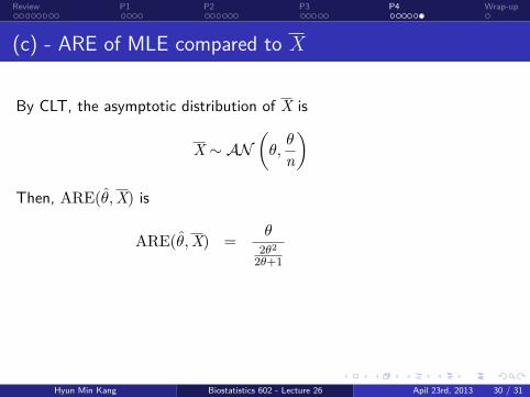
..........
.....
......
.....
.....
.....
......
.....
.....
.....
......
.....
.....
.....
......
.....
......
.....
.....
.
. . . . . . . .Review
. . . .P1
. . . . . .P2
. . . . .P3
. . . . . .P4
.Wrap-up
(c) - ARE of MLE compared to X
By CLT, the asymptotic distribution of X is
X ∼ AN(θ,
θ
n
)Then, ARE(θ,X) is
ARE(θ,X) =θ2θ2
2θ+1
=2θ + 1
2θ= 1 +
1
2θ> 1
Therefore, θ is more efficient estimator than X.
Hyun Min Kang Biostatistics 602 - Lecture 26 Apil 23rd, 2013 30 / 31
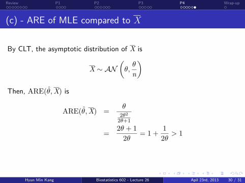
..........
.....
......
.....
.....
.....
......
.....
.....
.....
......
.....
.....
.....
......
.....
......
.....
.....
.
. . . . . . . .Review
. . . .P1
. . . . . .P2
. . . . .P3
. . . . . .P4
.Wrap-up
(c) - ARE of MLE compared to X
By CLT, the asymptotic distribution of X is
X ∼ AN(θ,
θ
n
)Then, ARE(θ,X) is
ARE(θ,X) =θ2θ2
2θ+1
=2θ + 1
2θ= 1 +
1
2θ> 1
Therefore, θ is more efficient estimator than X.
Hyun Min Kang Biostatistics 602 - Lecture 26 Apil 23rd, 2013 30 / 31
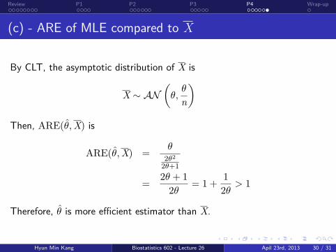
..........
.....
......
.....
.....
.....
......
.....
.....
.....
......
.....
.....
.....
......
.....
......
.....
.....
.
. . . . . . . .Review
. . . .P1
. . . . . .P2
. . . . .P3
. . . . . .P4
.Wrap-up
(c) - ARE of MLE compared to X
By CLT, the asymptotic distribution of X is
X ∼ AN(θ,
θ
n
)Then, ARE(θ,X) is
ARE(θ,X) =θ2θ2
2θ+1
=2θ + 1
2θ= 1 +
1
2θ> 1
Therefore, θ is more efficient estimator than X.
Hyun Min Kang Biostatistics 602 - Lecture 26 Apil 23rd, 2013 30 / 31

..........
.....
......
.....
.....
.....
......
.....
.....
.....
......
.....
.....
.....
......
.....
......
.....
.....
.
. . . . . . . .Review
. . . .P1
. . . . . .P2
. . . . .P3
. . . . . .P4
.Wrap-up
Wrapping Up
..1 Many thanks for your attentions and feedbacks.
..2 Please complete your teaching evaluations, which will be very helpfulfor further improvement in the next year.
..3 Final exam will be Thursday April 25th, 4:00-6:00pm.
..4 The last office hour will be held Wednesday April 24th, 4:00-5:00pm.
..5 The grade will be posted during the weekend.
..6 Don’t forget the materials we have learned, because they are the keytopics for your candidacy exam.
Hyun Min Kang Biostatistics 602 - Lecture 26 Apil 23rd, 2013 31 / 31