Bisection method in multiple dimensions

7/27/2019 Bisection method in multiple dimensions

http://slidepdf.com/reader/full/bisection-method-in-multiple-dimensions 1/6

Ŕ periodica polytechnica

Mechanical Engineering

56 / 2 (2012) 81 –86

doi: 10.3311 / pp.me.2012-2.01

web: http: // www.pp.bme.hu / me

c Periodica Polytechnica 2012

RESEARCH ARTICLE

Bisection method in higher dimensions

and the efficiency number

Dániel Bachrathy / Gábor Stépán

Received 2012-06-30

Abstract

Several engineering applications need a robust method to find

all the roots of a set of nonlinear equations automatically. The

proposed method guarantees monotonous convergence, and it

can determine whole submanifolds of the roots if the number of unknowns is larger than the number of equations. The critical

steps of the multidimensional bisection method are described

and possible solutions are proposed. An e fficient computational

scheme is introduced. The e fficiency of the method is charac-

terized by the box-counting fractal dimension of the evaluated

points. The multidimensional bisection method is much more ef-

ficient than the brute force method. The proposed method can

also be used to determine the fractal dimension of the submani-

fold of the solutions with satisfactory accuracy.

Keywords

Bisection method · multi dimension · system of non-linear

equations · multiple roots · e fficiency number

Acknowledgement

This work is connected to the scientific program of the “De-

velopment of quality-oriented and harmonized R+ D+ I strat-

egy and functional model at BME” project. This project is

supported by the New Széchenyi Plan (Project ID: TÁMOP-

4.2.1 / B-09 / 1 / KMR-2010-0002). The research leading to these

results has received funding from the European Union’s Seventh

Framework Programme (FP7 / 2007-2013) under grant agree-

ment n◦ 260073.

Dániel Bachrathy

HAS-BUTE Research Group on Dynamics of Machines and Vehicles, H-1111

Budapest, M ˝ uegyetem rkp. 5, Hungary

e-mail: [email protected]

Gábor StépánDepartment of Applied Mechanics, BME, H-1111 Budapest, M˝ uegyetem rkp.

5, Hungary

e-mail: [email protected]

1 Introduction

The bisection method – or the so-called interval halving

method – is one of the simplest root-finding algorithms which

is used to find zeros of continuous non-linear functions. This

method is very robust and it always tends to the solution if thesigns of the function values are diff erent at the borders of the

chosen initial interval. Unfortunately, it has only linear conver-

gence, more precisely, it doubles the accuracy with each itera-

tion, which is relatively slow. Hence, it is usually used to find

only a proper initial value for alternative root finding methods

which have better rate of convergence (e.g.: Newton’s method).

A big advantage of the bisection method is, however, that it can

be applied for non-diff erentiable continuous functions, too.

Geometrically, root-finding algorithms of f ( x) = 0 find one

intersection point of the graph of the function and the axis of the

independent variable. In many applications, this 1-dimensional

intersection problem must be extended to higher dimensions,

e.g.: intersections of surfaces in a 3D space (volume), which

can be described as a system on non-linear equations. In higher

dimensions, the existence of multiple solutions become very im-

portant, since the intersections of two surfaces can create mul-

tiple intersection lines. In this study, we give a description and

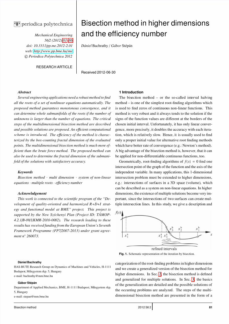
Fig. 1. Schematic representation of the iteration by bisection.

categorization of the root-finding problems in higher dimensions

and we create a generalized version of the bisection method for

higher dimensions. In Sec. 2, the bisection method is defined

and generalized for multiple solutions. In Sec. 3, the basics

of the generalization are detailed and the possible solutions of

the occurring problems are analyzed. The steps of the multi-

dimensional bisection method are presented in the form of a

Bisection method 812012 56 2

http://www.pp.bme.hu/me








flowchart (Fig. 4). Some hints for the numerical method are

given in Sec. 4. The computational efficiency of the method is

analyzed for diff erent problems in Sec. 5, based on numerical

results.

2 Bisection method

The bisection method is used to find the root of a nonlinear

real valued scalar function f ( x) = 0 ( f : R → R). The methodis initialized with the limits of an interval [ xa, xb], where the

function is defined (see Fig. 1). The signs of f ( xa) and f ( xb)

must be diff erent. In this case xa and xb are bracketing at least

one root, since, by the Intermediate Value Theorem, the function

f must have at least one zero in the interval ( xa, xb). At the

beginning of the iteration, the midpoint of the interval xc = ( xa+

xb)/2 is computed and f ( xc) is evaluated. If the sign of f ( xc) is

the same as the sign of f ( xa), then xc is set as a new value of

xa, otherwise, xc is set as a new value of xb and the iteration is

repeated. If xc happens to be a root of f (i.e., f ( xc) = 0) than the

iteration is completed in finite number of steps. In this process,

the length of the interval is reduced by 50% in each step, leading

to a strictly monotone linear convergence. The drawback of this

process is that it can find only one intersection point. In the next

subsection, a generalized version of this method is described,

which is able to find numerous roots.

2.1 Numerous solutions

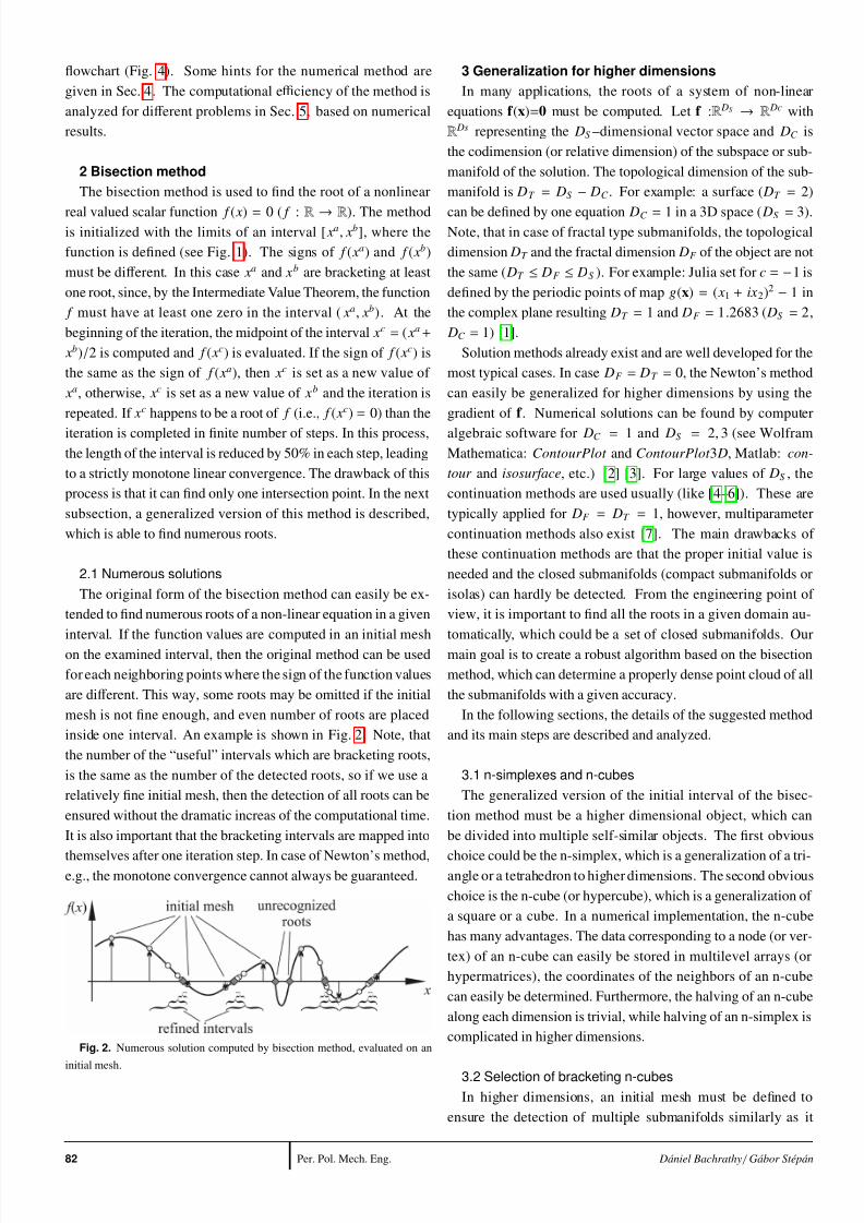
The original form of the bisection method can easily be ex-

tended to find numerous roots of a non-linear equation in a given

interval. If the function values are computed in an initial mesh

on the examined interval, then the original method can be used

for each neighboring points where the sign of the function values

are diff erent. This way, some roots may be omitted if the initial

mesh is not fine enough, and even number of roots are placed

inside one interval. An example is shown in Fig. 2. Note, that

the number of the “useful” intervals which are bracketing roots,

is the same as the number of the detected roots, so if we use a

relatively fine initial mesh, then the detection of all roots can be

ensured without the dramatic increas of the computational time.

It is also important that the bracketing intervals are mapped into

themselves after one iteration step. In case of Newton’s method,e.g., the monotone convergence cannot always be guaranteed.

Fig. 2. Numerous solution computed by bisection method, evaluated on an

initial mesh.

3 Generalization for higher dimensions

In many applications, the roots of a system of non-linear

equations f (x)=0 must be computed. Let f :R DS → R Dc with

R Ds representing the DS –dimensional vector space and DC is

the codimension (or relative dimension) of the subspace or sub-

manifold of the solution. The topological dimension of the sub-

manifold is DT = DS − DC . For example: a surface ( DT = 2)

can be defined by one equation DC = 1 in a 3D space ( DS = 3).Note, that in case of fractal type submanifolds, the topological

dimension DT and the fractal dimension DF of the object are not

the same ( DT ≤ DF ≤ DS ). For example: Julia set for c = −1 is

defined by the periodic points of map g(x) = ( x1 + ix2)2 − 1 in

the complex plane resulting DT = 1 and DF = 1.2683 ( DS = 2,

DC = 1) [1].

Solution methods already exist and are well developed for the

most typical cases. In case DF = DT = 0, the Newton’s method

can easily be generalized for higher dimensions by using the

gradient of f . Numerical solutions can be found by computer

algebraic software for DC = 1 and DS = 2, 3 (see Wolfram

Mathematica: ContourPlot and ContourPlot 3 D, Matlab: con-

tour and isosurface, etc.) [2] [3]. For large values of DS , the

continuation methods are used usually (like [4–6]). These are

typically applied for DF = DT = 1, however, multiparameter

continuation methods also exist [7]. The main drawbacks of

these continuation methods are that the proper initial value is

needed and the closed submanifolds (compact submanifolds or

isolas) can hardly be detected. From the engineering point of

view, it is important to find all the roots in a given domain au-

tomatically, which could be a set of closed submanifolds. Our

main goal is to create a robust algorithm based on the bisection

method, which can determine a properly dense point cloud of all

the submanifolds with a given accuracy.

In the following sections, the details of the suggested method

and its main steps are described and analyzed.

3.1 n-simplexes and n-cubes

The generalized version of the initial interval of the bisec-

tion method must be a higher dimensional object, which can

be divided into multiple self-similar objects. The first obvious

choice could be the n-simplex, which is a generalization of a tri-angle or a tetrahedron to higher dimensions. The second obvious

choice is the n-cube (or hypercube), which is a generalization of

a square or a cube. In a numerical implementation, the n-cube

has many advantages. The data corresponding to a node (or ver-

tex) of an n-cube can easily be stored in multilevel arrays (or

hypermatrices), the coordinates of the neighbors of an n-cube

can easily be determined. Furthermore, the halving of an n-cube

along each dimension is trivial, while halving of an n-simplex is

complicated in higher dimensions.

3.2 Selection of bracketing n-cubes

In higher dimensions, an initial mesh must be defined to

ensure the detection of multiple submanifolds similarly as it

Per. Pol. Mech. Eng.82 Dániel Bachrathy / Gábor Stépán



was shown in Sec. 2.1. First, two limit value xa j and xb

j and

the size of the mesh N j must be defined for each dimension

( j ∈ {1, 2,... DS }). The edge length of the initialized n-cube in

the jth dimension is ∆ x j = ( xb j − xa

j )/( N j −1). In the next step, the

function value must be computed in all the DS

j=1N j points. Be-

fore the refinement, the bracketing n-cubes which contain parts

of the submanifold must be selected from all the initialized n-

cubes. This step also has to be modified in case DC > 1 accord-ing to the given problem.

Safe selection

If the sign of f k is diff erent at any two nodes of an n-cube for

all k = 1, 2,... DC , then it is possible, that the n-cube brackets

a part of a submanifold. Unfortunately, this is just a necessary

condition, however, this condition can be used to define the n-

cube as a bracketing one. In this case, non-bracketing n-cubes

will be also selected and refined. This does not lead to computa-

tional error if further analysis or iteration is applied, because for

smaller refined n-cubes, the apparent bracketing will disappear.

The only minor problem is that the unnecessary selections will

increase the computational time.

Secant based selection

A more precise selection of the bracketing n-cubes is based

on the secant method. In this case, the submanifold inside the n-

cube is to be found by linear interpolations. The iteration starts

with connecting all the nodes with positive f 1 values to all the

nodes with negative f 1 values, then the roots of f 1 along these

lines are linearly approximated by the secant method. Then, f

is linearly interpolated in these points. The iteration is repeated

for f 2, f 3,...and f DC . If in any stage of the iteration, the sign of

f k are the same in all interpolated points, then the next step of

the iteration is impossible, which means that the current n-cube

is non-bracketing. If an exact 0 is found, then it is a bracketing

n-cube.

Fitting hyper-planes

Another possible solution is to fit a hyper-plane to the func-

tion values of the nodes at the current n-cube. The normal vec-

tors of the hyper-plane can be computed as well as the closestpoint of the hyper-plane to the center of the n-cube. If this point

is “close enough” to the n-cube then it can be selected as a brack-

eting cube, since it will be a bracketing n-cube indeed, with high

probability.

An advantage of the selection methods presented in this sub-

section is that the additional evaluation of f is unnecessary.

Other types of selection methods could be created if we com-

pute f at additional points.

The appropriate method of the selection depends on the given

problem. The safe selection is very fast, but the computational

time increases if the codimension-1 surfaces ( f j( x) = 0) are al-

most parallel at the intersection points. However, it is still ad-

vised to use it if the evaluation of f is fast enough. In this case

the selection of the bracketing n-cubes can be the bottleneck of

the computation. Otherwise, if the evaluation of f is slow, then

the selection based on the secant method or the fitting of hyper-

plane give better performance. Based on our experiments, if

DS < 4 then the secant based selection is faster than fitting a

hyper-plane. Still, these two methods give poor results if the

curvatures of the surfaces are relatively large compared to the

size of the n-cube. These two methods could possibly mark abracketing n-cube as a non-bracketing one which could lead to

the loss of some parts of the submanifold.

If DT ≥ 1, the missing parts of the submanifold can be found

by using some kind of continuation method at the very end of

the iteration.

3.3 Continuation – neighboring n-cubes

At the end of the iterations all the neighbors of the bracketing

n-cubes must be examined. If additional bracketing n-cubes are

found then a missing part of the submanifold is detected. These

tests should be repeated till all the neighboring n-cubes of the

bracketing n-cubes are non-bracketing. In this case, the whole

submanifold is found in the selected region. This method is sim-

ilar to a multiparameter continuation method, because if a small

part of the submanifold is detected, then it is extended during

the iterations until it is closed into itself (in case of an isola) or

until the boundary of the selected range is reached.

This continuation method is very efficient, because the evalu-

ation of f is carried out only along the submanifold.

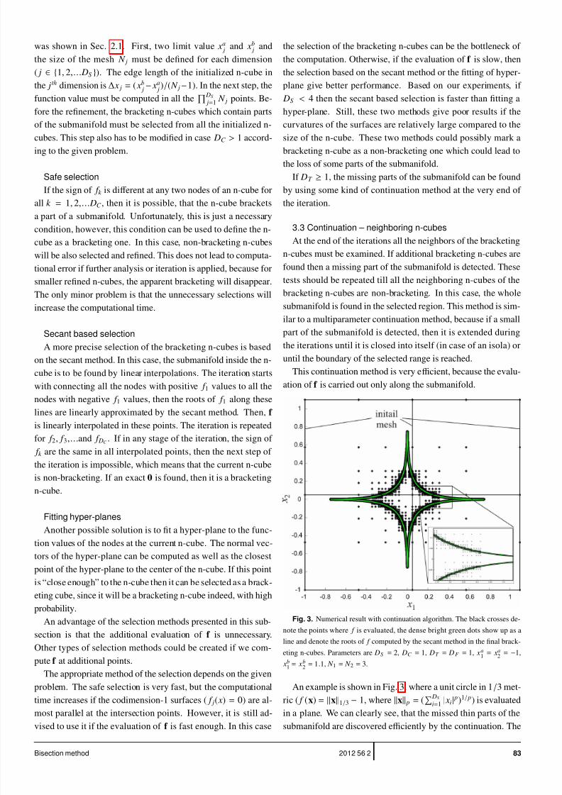
Fig. 3. Numerical result with continuation algorithm. The black crosses de-

note the points where f is evaluated, the dense bright green dots show up as a

line and denote the roots of f computed by the secant method in the final brack-

eting n-cubes. Parameters are DS = 2, DC = 1, DT = DF = 1, xa1= xa

2= −1,

xb1= xb

2= 1.1, N 1 = N 2 = 3.

An example is shown in Fig. 3, where a unit circle in 1/3 met-

ric ( f (x) = x1/3 − 1, where x p = (

DS i=1

| xi| p)1/ p) is evaluated

in a plane. We can clearly see, that the missed thin parts of the

submanifold are discovered efficiently by the continuation. The




examination of the neighbouring cubes is not necesseary in all

cases since it slightly increases the computational time.

The final step of the method is the interpolation of the roots

inside the bracketing n-cubes, which can be done by the secant

method, the hyper-plane fitting or other more advanced meth-

ods. Now, all the necessary steps of the proposed algorithm are

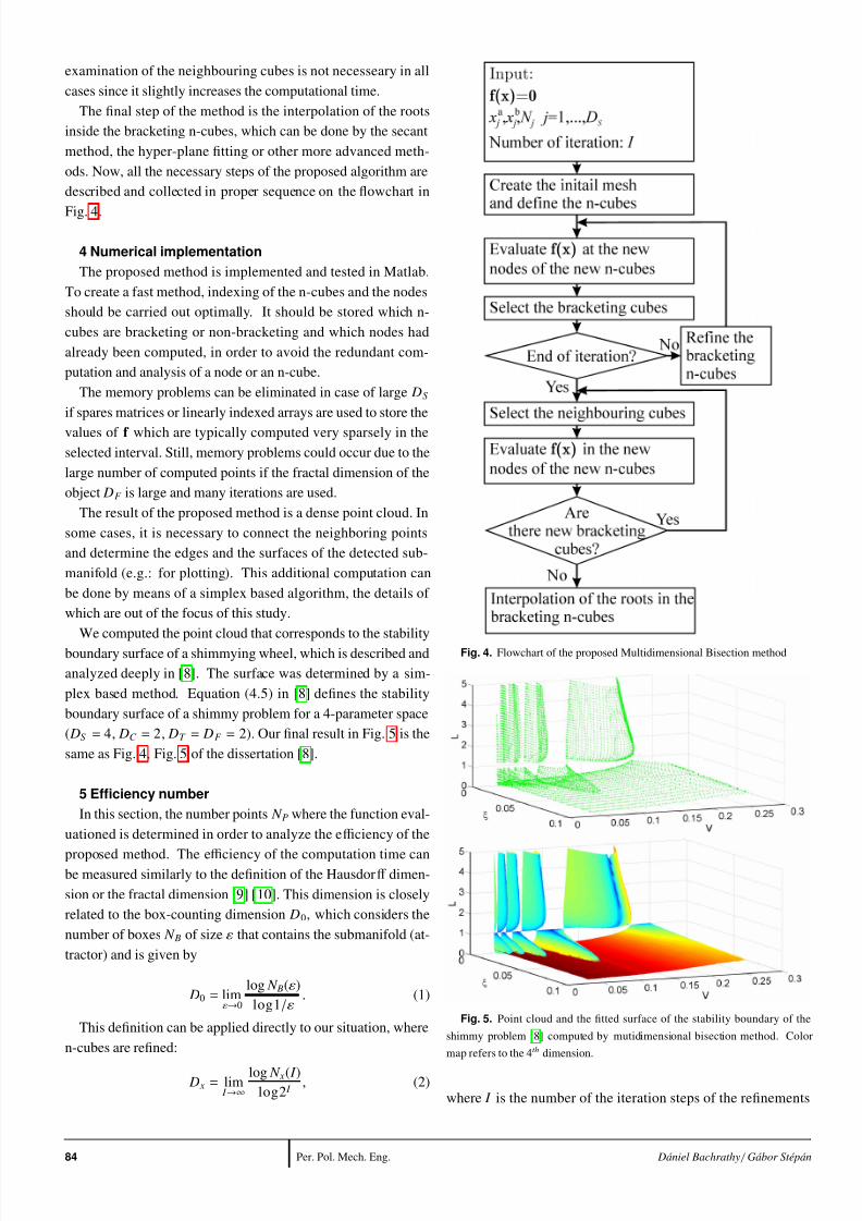
described and collected in proper sequence on the flowchart in

Fig. 4.

4 Numerical implementation

The proposed method is implemented and tested in Matlab.

To create a fast method, indexing of the n-cubes and the nodes

should be carried out optimally. It should be stored which n-

cubes are bracketing or non-bracketing and which nodes had

already been computed, in order to avoid the redundant com-

putation and analysis of a node or an n-cube.

The memory problems can be eliminated in case of large DS

if spares matrices or linearly indexed arrays are used to store the

values of f which are typically computed very sparsely in the

selected interval. Still, memory problems could occur due to the

large number of computed points if the fractal dimension of the

object DF is large and many iterations are used.

The result of the proposed method is a dense point cloud. In

some cases, it is necessary to connect the neighboring points

and determine the edges and the surfaces of the detected sub-

manifold (e.g.: for plotting). This additional computation can

be done by means of a simplex based algorithm, the details of

which are out of the focus of this study.

We computed the point cloud that corresponds to the stability

boundary surface of a shimmying wheel, which is described and

analyzed deeply in [8]. The surface was determined by a sim-

plex based method. Equation (4.5) in [8] defines the stability

boundary surface of a shimmy problem for a 4-parameter space

( DS = 4, DC = 2, DT = DF = 2). Our final result in Fig. 5 is the

same as Fig. 4, Fig. 5 of the dissertation [8].

5 Efficiency number

In this section, the number points N P where the function eval-

uationed is determined in order to analyze the efficiency of the

proposed method. The efficiency of the computation time canbe measured similarly to the definition of the Hausdorff dimen-

sion or the fractal dimension [9] [10]. This dimension is closely

related to the box-counting dimension D0, which considers the

number of boxes N B of size ε that contains the submanifold (at-

tractor) and is given by

D0 = limε→0

log N B(ε)

log1/ε. (1)

This definition can be applied directly to our situation, where

n-cubes are refined:

D x = lim I →∞

log N x( I )log2 I

, (2)

Fig. 4. Flowchart of the proposed Multidimensional Bisection method

Fig. 5. Point cloud and the fitted surface of the stability boundary of the

shimmy problem [8] computed by mutidimensional bisection method. Color

map refers to the 4th dimension.

where I is the number of the iteration steps of the refinements




of the n-cubes. If we substitute N x with the number of brack-

eting cubes then the fractal dimension of the submanifold DF

is determined, but if the number of function evaluation N P is

substituted, then we get the fractal dimension of the evaluated

points DP. This number shows, how dense the evaluated points

are in the space. We define the efficiency number E of the com-

putation method as follows.

E =1

DP − DF . (3)

First, look at the so-called “brute force method”, where the

function is evaluated at all points in the final mesh for which N Pis given by

N P =

DS

j=1

N j − 1

2 I + 1

≈2 I DS

DS

j=1

N j. (4)

It is clear, that for the brute force method, the fractal dimension

of the evaluated points DP tends rapidly to the dimension of

the whole vectorspace DS , which leads to a small value of the

efficiency number E = 1/( DS − DF ). Note, that E = 1/ DC in

case of non-fractal type manifolds.

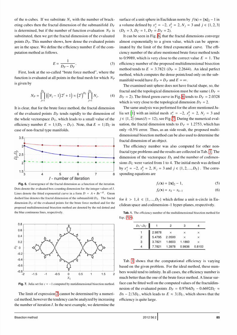
Fig. 6. Convergence of the fractal dimension as a function of the iteration.

Dots denote the evaluated box-counting dimension for the integer values of I .

Lines denote the fitted exponential curve in a form D = A + Be−λ I . Green

dashed line denotes the fractal dimension of the submanifold DS . The fractal

dimension DP of the evaluated points for the brute force method and for the

proposed multidimensional bisection method are denoted by the red dotted and

the blue continuous lines, respectively.

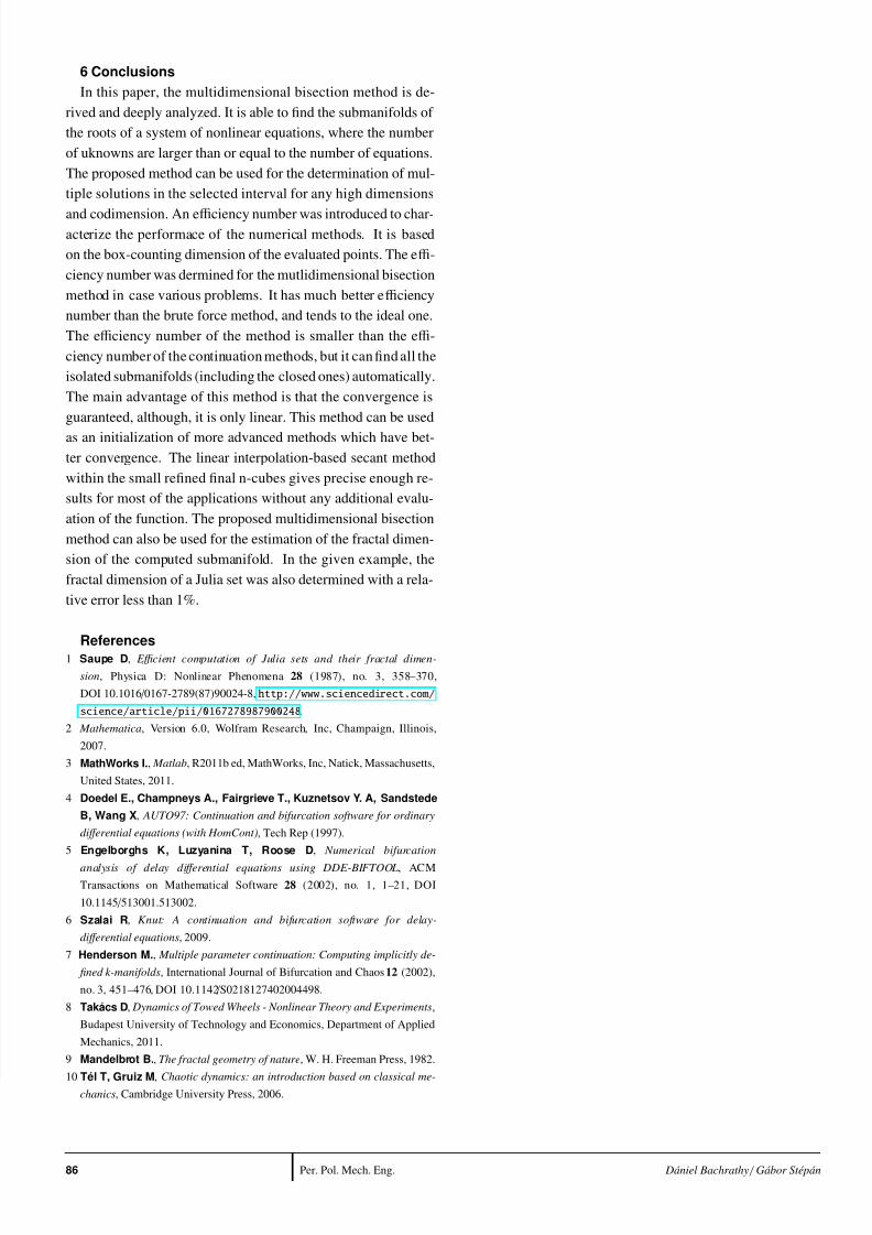
Fig. 7. Julia set for c = −1 computed by mutidimensional bisection method.

The limit of expression 2 cannot be determined by a numeri-cal method, however the tendency can be analyzed by increasing

the number of iteration I . In the next example, we determine the

surface of a unit sphere in Euclidean norm by f (x) = x2 − 1 in

a volume defined by xa j = −2, xb

j = 2, N j = 3 and j ∈ {1, 2, 3}

( DS = 3, DC = 1, DT = DF = 2).

It can be seen in Fig. 6, that the fractal dimensions converge

almost exponentially to a given value, which can be approx-

imated by the limit of the fitted exponential curve. The effi-

ciency number of the afore mentioned brute force method tends

to 0.9989, which is very close to the correct value E = 1. Theefficiency number of the proposed multidimensional bisection

method tends to E = 3.7821 ( DP = 2.2644). An ideal perfect

method, which computes the dense pointcloud only on the sub-

manifold would have DP = DF and E = ∞.

The examined unit sphere does not have fractal shape, so, the

fractal and the topological dimension must be the same ( DT =

DF = 2). The fitted green curve in Fig. 6 tends to DF = 2.0328

which is very close to the topological dimension DT = 2.

The same analysis was performed for the afore mentioned Ju-

lia set [1] with an initial mesh xa j = −2, xb

j = 2, N j = 3 and

j ∈ {1, 2} (max( I ) = 12), see Fig. 7. During the numerical eval-

uation, the fractal dimension tends to DF = 1.2753, which has

only ~0.5% error. Thus, as an side result, the proposed multi-

dimensional bisection method can be also used to determine the

fractal dimension of an object.

The efficiency number was also computed for other non-

fractal type problems and the results are collected in Tab. 1. The

dimension of the vectorspace DS and the number of codimen-

sions DC were varied from 1 to 4. The initial mesh was defined

by xa j = −2, xb

j = 2, N j = 3 and j ∈ {1, 2, ..., DS } . The corre-

sponding equations are

f 1(x) = x2 − 1, (5)

f k (x) = xk − xk −1 (6)

for k > 1, k ∈ {1, ..., DC } which define a unit n-circle in Eu-

clidean space and codimension–1 hyper-planes, respectively.

Tab. 1. The efficiency number of the multidimensional bisection method for

Eqs. (5, 6).

DS DC 1 2 3 4

1 2.9878 × × ×

2 5.4795 2.0500 × ×

3 3.7821 1.6603 1.1860 ×

4 7.7821 1.3978 0.9936 0.8103

Tab. 1 shows that the computational efficiency is varying

based on the given problem. For the ideal method, these num-

bers would tend to infinity. In all cases, the efficiency number is

much better than the one of the brute force method. A linear sur-

face can be fitted well on the computed values of the fractaldim-

nesion of the evaluated points DP = 0.9764 DS − 0.6692 DC ≈

Ds − 2/3 DC , which leads to E ≈ 3/ DC , which shows that theefficiency is quite large.




6 Conclusions

In this paper, the multidimensional bisection method is de-

rived and deeply analyzed. It is able to find the submanifolds of

the roots of a system of nonlinear equations, where the number

of uknowns are larger than or equal to the number of equations.

The proposed method can be used for the determination of mul-

tiple solutions in the selected interval for any high dimensions

and codimension. An efficiency number was introduced to char-acterize the performace of the numerical methods. It is based

on the box-counting dimension of the evaluated points. The effi-

ciency number was dermined for the mutlidimensional bisection

method in case various problems. It has much better efficiency

number than the brute force method, and tends to the ideal one.

The efficiency number of the method is smaller than the effi-

ciency number of the continuation methods, but it can find all the

isolated submanifolds (including the closed ones) automatically.

The main advantage of this method is that the convergence is

guaranteed, although, it is only linear. This method can be used

as an initialization of more advanced methods which have bet-

ter convergence. The linear interpolation-based secant method

within the small refined final n-cubes gives precise enough re-

sults for most of the applications without any additional evalu-

ation of the function. The proposed multidimensional bisection

method can also be used for the estimation of the fractal dimen-

sion of the computed submanifold. In the given example, the

fractal dimension of a Julia set was also determined with a rela-

tive error less than 1%.

References

1 Saupe D, E fficient computation of Julia sets and their fractal dimen-

sion, Physica D: Nonlinear Phenomena 28 (1987), no. 3, 358–370,

DOI 10.1016 / 0167-2789(87)90024-8, http://www.sciencedirect.com/

science/article/pii/0167278987900248.

2 Mathematica, Version 6.0, Wolfram Research, Inc, Champaign, Illinois,

2007.

3 MathWorks I., Matlab, R2011b ed, MathWorks, Inc, Natick, Massachusetts,

United States, 2011.

4 Doedel E., Champneys A., Fairgrieve T., Kuznetsov Y. A, Sandstede

B, Wang X, AUTO97: Continuation and bifurcation software for ordinary

di ff erential equations (with HomCont), Tech Rep (1997).

5 Engelborghs K, Luzyanina T, Roose D, Numerical bifurcation

analysis of delay di ff erential equations using DDE-BIFTOOL, ACM

Transactions on Mathematical Software 28 (2002), no. 1, 1–21, DOI

10.1145 / 513001.513002.

6 Szalai R, Knut: A continuation and bifurcation software for delay-

di ff erential equations, 2009.

7 Henderson M., Multiple parameter continuation: Computing implicitly de-

fined k-manifolds, International Journal of Bifurcation and Chaos 12 (2002),

no. 3, 451–476, DOI 10.1142 / S0218127402004498.

8 Takács D, Dynamics of Towed Wheels - Nonlinear Theory and Experiments,

Budapest University of Technology and Economics, Department of Applied

Mechanics, 2011.

9 Mandelbrot B., The fractal geometry of nature, W. H. Freeman Press, 1982.

10 Tél T, Gruiz M, Chaotic dynamics: an introduction based on classical me-chanics, Cambridge University Press, 2006.


http://www.sciencedirect.com/science/article/pii/0167278987900248





Documents

Bisection method in multiple dimensions