Bisectored Unit Disk Graphs

John NolanMathematical Institute, 24-29 St Giles’, University of Oxford, OX1 3LB, United Kingdom

Unit disk graphs form a natural model for cellular radiochannel assignment problems under the assumption ofequally powerful, omnidirectional transmitters locatedon a uniform, flat plane. Here, we introduce and givemotivation for an extension of this model, namely, sec-torization at transmitter sites. We define and analyzeproperties of one case of sectorization, bisectored unitdisk graphs, in particular, investigating properties con-cerning their chromatic number. Finally, we providesome experimental evidence to draw comparisons be-tween graphs of this model and other classes of graphs.© 2004 Wiley Periodicals, Inc.

Keywords: channel assignment; frequency assignment; unitdisk graphs; colorings

1. INTRODUCTION

A unit disk graph (UDG) is the intersection graph of a setof unit disks on the Euclidean plane. Imagine that we havea network N of equally powerful ratio transmitters on theplane, and for each transmitter, we can, in some way,represent its cellular broadcast range with a unit disk. LetG(N) be the corresponding UDG of these disks. Assumethat the available radio spectrum for these transmitters is afinite set � of k :� ��� distinct frequencies, from whicheach transmitter must use precisely one. Our only restrictionis that whenever two transmitters are close to each other,that is, their disks intersect, they must broadcast on differentfrequencies (this is a co-channel restraint). Then, it is clearthat there exists a valid assignment of frequencies from � toall the transmitters of N if and only if the graph G(N) isk-colorable. We are particularly interested in keeping thevalue of k low, as the effects of spectrum regulation andmarket forces mean that any extra spectrum is always dif-ficult to acquire.

This example demonstrates one application of the color-

ing of intersection graphs. Among the models with relatedconstructions are the classes of disk graphs (a more generaland difficult-to-handle model where individual disk sizescan vary) and sphere-of-influence graphs.* However wewill only consider an extension to the UDG model here.

In reality, the UDG model makes several restrictiveassumptions. One of these is that there is only a singletransmitter at each site. This paper explores properties of amodel where each site has two aligned transmitters, pavingthe way toward more realistic models of cellular networks.The broadcast range at each site is partitioned into twoequal-sized sectors, each served by its own transmitter.

1.1. Preliminaries

Suppose that G is a graph. We denote the vertex set of Gby V(G) and the edge set by E(G). If u, v � V(G), we usethe shorthand u � v to mean that u is adjacent to v. We willonly consider simple, finite graphs in this paper. The neigh-borhood of a vertex v, denoted N(v), is the set of vertices inG that are adjacent to v, while the degree of v, d(v), isequal to the number of edges incident to v (i.e., �N(v)� for allthe graphs that we consider). We use �(G) for the maxi-mum degree over all vertices in G, and �(G), for theminimum degree. The complement of G, denoted G� , is thegraph obtained by taking V(G� ) � V(G) and placing an edgebetween vertices u and v in G� if and only if u � v in G.

H is a subgraph of G if H is a graph with V(H) � V(G)and E(H) � E(G). Define �*(G) :� max �(H) over allsubgraphs H of G. Suppose that S � V(G): Then, the graphinduced by S is the graph H with V(H) � S, and for all u,v � S, u � v in H if and only if u � v in G. A clique isa set of pairwise adjacent vertices (the graph consisting onlyof a clique on n vertices, called a complete graph, is denotedby Kn). The null graph Nn is defined as K� n. The clique sizeof G, �(G), is the size of the largest clique that is asubgraph of G. G is k-colorable if one can assign a color to

Received December 2002; accepted October 2003Correspondence to: J. Nolan; e-mail: nolan@maths.ox.ac.ukContract grant sponsors: Engineering and Physical Sciences ResearchCouncil; Radiocommunications Agency; and Smith Institute for IndustrialMathematics and System Engineering

© 2004 Wiley Periodicals, Inc.

* Given a set of n points on the plane, center a disk at each point with theradius equal to the distance between the point and its nearest neighbor. Theresulting intersection graph is a sphere-of-influence graph (SIG). Althoughthese graphs intuitively seem to model a type of coverage network, the factthat dense networks and large cliques are prohibited makes them undesir-able for our purposes—see [10] for more information about SIGs.

NETWORKS, Vol. 43(3), 141–152 2004

each vertex of G using k colors, so that no two adjacentvertices have the same color. A k-coloring is such an as-signment to a k-colorable graph. The chromatic number,�(G), is the minimum k for which a k-coloring exists.

An independent set I � V(G) is a set of vertices suchthat the induced subgraph on I has no edges. A graph G isbipartite if there exist disjoint independent sets A and Bsuch that A � B � V(G). The complete bipartite graph,Ki, j, is a graph with this property such that �A� � i, �B� �j and there is an edge between each vertex of A and eachvertex of B.

A circuit, Cn (for n � 2), is the connected graph with nvertices and n edges, with each vertex having degree 2.Graph G is perfect if, for every induced subgraph H of G,�(H) � �(H) (see [7] for more information about this classof graphs). An orientation of G is an assignment of adirection to every edge of G, so if a � b, then either a 3b or b 3 a (for all pairs of vertices a, b). G is acomparability graph if there exists an orientation on theedges of G such that if u 3 v and v 3 w then (u � w and)u 3 w, that is, a transitive orientation. A co-comparabilitygraph is the complement of a comparability graph.

We say that a graph G is a unit disk graph if there existsa function f : V(G) 3 �2 such that @u, v � V(G), u � vN d( f(u), f(v)) � h, where d represents the usual Euclid-ean distance and h is a positive constant. Sometimes, wewill talk about a unit disk graph being given with itsrepresentation: This means that such a function f (and avalue h) is explicitly provided. We will use G* to denote agraph that comes with this information (we will sometimesabuse notation to allow G* to refer to the graph or therepresentation). Note that the initial choice of h is arbitrary,in the sense that it will always define the same class ofgraphs, because distances in the representation can bescaled. In fact, we will use the value h � � � 1, whosevalue will be explained later.

If u and v are vertices, we use the notation d(u, v) tomean the Euclidean distance between the sites of u and vwhen a representation is available. Similarly, ux and uy willrefer to the x- and y-coordinates of the location of u in therepresentation. We also use a few terms from complexitytheory in this paper—rather than give precise definitionshere, the reader is referred to [4].

1.2. Background on Unit Disk Graphs

Finding the chromatic number of unit disk graphs is anNP-Hard problem (see [3, 5]). This is true even if the graphis supplied with its representation. On the other hand, [3]also shows that the clique number of a UDG can always becalculated in polynomial time (in fact, this can be done evenwithout the representation [14]).

This imbalance raises the question of whether the chro-matic number can in some way be bounded by a multiple ofthe clique number. We know that this is not the case forgraphs in general (e.g., [12]). It turns out to be straightfor-ward to show that � � 6� � 6 for UDGs, using a bound on

� (see, e.g., [5]). This stronger result that � � 3� � 2 wasfirst shown in [13], using a lexicographical ordering of thevertices before applying the greedy algorithm. This is stillthe best-known bound. In fact, a coloring satisfying thisbound can be found in fast time without a representation ofthe UDG, the same result that we use in Corollary 2.

After we have defined bisectored unit disk graphs(BUDGs), we will be explicit in stating whether or not aBUDG is given with its representation. This is because [2]shows that recognizing a graph as a UDG is an NP-Hardproblem, and it is very likely that this is true also forBUDGs.

2. MODELING ACCEPTABLE SIGNALRECEPTION IN A COVERAGE NETWORK

We will step back from UDGs for the moment to brieflydiscuss when it is necessary for two transmitters to broad-cast on different frequencies in a network. This will allow usto define reuse distances for the model—(maximum) dis-tances below which two vertices on the plane must beadjacent, from which we can define our bisectored unit diskgraph model.

Let X be a transmitter. We will assume throughout thateach transmitter broadcasts at just one frequency (although,in reality, this may represent a block of frequencies) anddifferent transmitters always broadcast different signals (al-though they may broadcast at the same frequency). Let � bethe set of all points on �2 for which we need acceptablereception of the signal broadcast from X (we say that � isthe coverage area of X). Let Y be another transmitter on theplane with coverage area �—this transmitter is a potentialsource of interference to X. One way to guarantee nointerference in our cochannel restraint model would be toforce X and Y to broadcast on different frequencies. How-ever, to use the frequency spectrum efficiently, we want toenforce this only where absolutely necessary: There may bemany transmitters and assigning each their own frequencywill not be feasible.

We will assume throughout this paper that the terrain onthe plane is homogeneous and that transmitters are equallypowerful. Hence, differences in the strengths of receivedsignals depend only on the distances to the transmitters.However, we will permit transmitters to be directed: Theycan broadcast a full signal in some angular directions and nosignal in others. So, for x � �2, let dY( x) denote theEuclidean distance between x and transmitter Y, with theexception that if Y is a directional antenna and x does not liein its angular broadcast sector then we will take dY( x) � �.Similarly, define dX( x) for transmitter X. Then, we will saya point x � � can receive an acceptable signal from Xwhen Y uses the same frequency if and only if

�dY x

dX x��

� .

Here, the constant represents the signal technology: It will

142 NETWORKS—2004

take a low value for voice applications, but a much highervalue for data transmissions (where errors are far morecrucial). As an example, typical GSM networks use a valueof between 9 and 14 decibels. The other constant, �,represents the propagation environment. Propagation in freespace would give � a value of two, but more practical forapplications is a value of around four, reaching as high assix for heavily built up areas.

We call the ratio dY( x)/dX( x) the interference-to-signaldistance ratio at x. In what follows, we will let � :� 1/�.(For example, a network where is 14 dB and � is 4 wouldgive � a value of 2.239.) Define the relationship � (ontransmitters) to mean “potentially interferes with”, that is,must broadcast on different frequencies. Then, we have

X � Y N � x � � such that dYx � � dXx or y � � such that dXy � �dYy. (1)

For bisectored unit disk graphs, we will define the coverageareas to be the set of points lying inside the angular sectorof broadcast and within radius 1 of the source transmitter.

3. DEFINITION OF SECTORED UNIT DISKGRAPHS

First, we fix � :� 1/� to be a constant such that � � �2(this is for technical reasons). The following definitions areimplicitly dependent on this value of �.

A k-sectored unit disk graph is defined to be a graph Gthat can be represented (using a suitable choice of variables)as follows: Let p1, . . . , pn be n distinct points (representingsites) on �2. For each point, let Di denote the disk of radiusone centered at pi and let �i � [0, 2 ). Divide each diskDi into k equally sized sectors: Let Si, j refer to the sector ofDi over the angle [�i � 2 ( j � 1)/k, �i � 2 j/k] at pi

(measured from some global reference angle), for 1 � i� n and 1 � j � k. Notice that the sectors at each site aredisjoint except for the radial lines that form their bound-aries. Associate a vertex vi, j with each sector Si, j: Theseform the vertex set of G and represent the different trans-mitters. For each i, we set the vertices vi,1, . . . , vi,k to bepairwise adjacent, so the transmitters at the same site areforced to use different frequencies. Now regard each vertexvi, j to be a directional antenna, located at pi, broadcastingonly in the direction of the angle range of Si, j and withcoverage area equal to Si, j. Then, for any pair of transmit-

ters at different sites, we determine if the vertices areadjacent using (1).

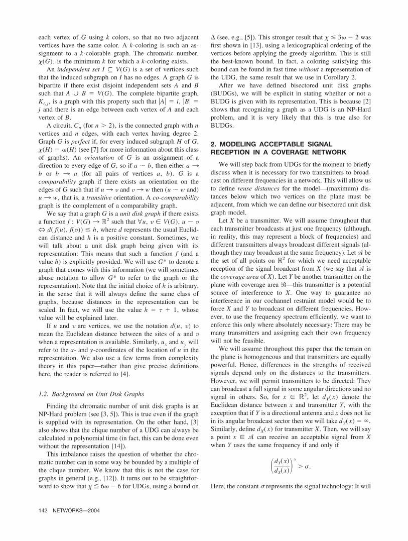
Our first definition of a bisectored unit disk graph (orBUDG) is as a two-sectored unit disk graph for which �i

� �1 for all i. Without loss of generality, we take �1 to bethe angle of the (horizontal) x-axis and refer to the twoopposite facing classes of sectors as north and south. Figure1 demonstrates this idea. Note that each vertex is effectivelya transmitter, so we will use the two terms interchangeablydepending on the context.

We now explore the reuse distances a little further todefine BUDGs more explicitly. Our method of calculatingreuse distances follows directly from (1): Suppose that Xand Y are transmitters whose sites lie distance r apart withfixed angles � between them (we use the acute angle fromthe sectors’ boundary). Given the respective coverage areas� and � of the two transmitters, we find a point in � � �which has lowest interference-to-signal distance ratio. So, ifthis critical point can receive an acceptable signal when Xand Y use the same frequency, then all points in bothcoverage areas can.

Assume, without loss of generality, that the critical pointis a � �. Then, the reuse distance is given by solving

dYa � �dXa in r. (2)

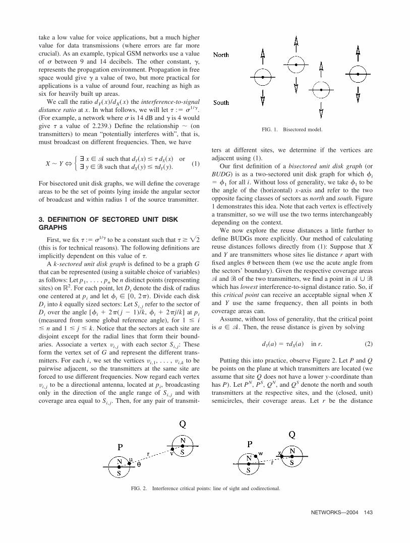
Putting this into practice, observe Figure 2. Let P and Qbe points on the plane at which transmitters are located (weassume that site Q does not have a lower y-coordinate thanhas P). Let PN, PS, QN, and QS denote the north and southtransmitters at the respective sites, and the (closed, unit)semicircles, their coverage areas. Let r be the distance

FIG. 1. Bisectored model.

FIG. 2. Interference critical points: line of sight and codirectional.

NETWORKS—2004 143

between P and Q, and �, the (acute) angle between themfrom the sectors’ boundary. For now, we assume that thecoverage areas of the different sites do not intersect eachother.

By definition, we have PN � PS and QN � QS and it isclear, provided that � � 0, that PS � QN. Now, weidentify the critical points for the remaining cases. Forthe pair PN, QS (line of sight), it is straightforward to seethat it is u (or, equivalently, v) that is both furthest fromits source transmitter and closest to the interfering trans-mitter. On the other hand, for PN, QN (a codirectionalpair), we have two candidates for the critical point: x orw. However, it turns out that x is critical for all � and �� 1. So, using R to denote the reuse distance obtained bysolving Eq. (2) in r gives

RPN, QN � RPS, QS :� ��2 � sin2� � cos �,

RPN, QS :� � � 1.

The exception is when � � 0, which, by virtue of allsectors being closed, leads to all four intersite transmitterpairs having reuse distance � � 1. Observe that R(PN, QS)� R(PN, QN) always, with equality only at this particularangle.

Finally, by insisting that � � �2, these reuse distancesare guaranteed to correctly determine adjacency even whenthe two coverage areas do intersect. Converting this infor-mation into Cartesian coordinates gives us the desired ex-plicit definition.

3.1. Definition of Bisectored Unit Disk Graph

First, fix � :� 1/� � �2. A bisectored unit disk graphrepresentation on n sites is a set ( x1, y1), ( x2, y2), . . . ,( xn, yn) of distinct points in �2 with associated vertices v1

N,v2

N, . . . , vnN and v1

S, v2S, . . . , vn

S such that

1. viN � vi

S,2. vi

N � vjS N dy � 0 and dx

2 � dy2 � (� � 1)2,

3. viN � vj

N and viS � vj

S N (�dx� � 1)2 � dy2 � �2,

4. Vertices are nonadjacent otherwise,

for all distinct i and j with 1 � i, j � n, where dx :� xj

� xi and dy :� yj � yi. A graph is a bisectored unit diskgraph if it has such a representation.

3.2. Sectorization Transformation

We define a transformation � which provides a simplemodel of a switch from a network with omnidirectionalantennas (UDGs) to a network where each site has twodirectional antennas (BUDGs). The main assumptions arethat the same transmitter sites are used, the total transmittingpower at each site is the same (the sites are now split into

north and south transmitters, but the power density is thesame as before in all directions), and the boundaries of thedirected antennas are aligned with each other.

When using omnidirectional transmitters, interference isdefined by the line of sight reuse distance, � � 1. So, a UDGmay be viewed as a model of a cellular omnidirectionaltransmitter network with each transmitter having range h/(�� 1) (recall that h is the arbitrary fixed distance belowwhich two vertices are adjacent in a UDG)—so, by ourchoice of h :� � � 1, the range become of unit length, thesame as those of BUDGs.

We define � � �(G*, �) to act on a representation ofa UDG (i.e., a set of n points in the plane and a constant h� � � 1) and return a bisectored unit disk graph with itsrepresentation. Here, � � [0, 2 ) represents the orientationof all the sector borders with respect to the UDG represen-tation. So � takes the locations of the vertices of G*, rotatesthem by � about the origin, and uses these and the value �to create the representation of a BUDG following the pre-vious definition. In fact, we will assume that � � 0 since allit represents is a simple rotation in the representation, so wewill talk about � operating on just a representation of aUDG.

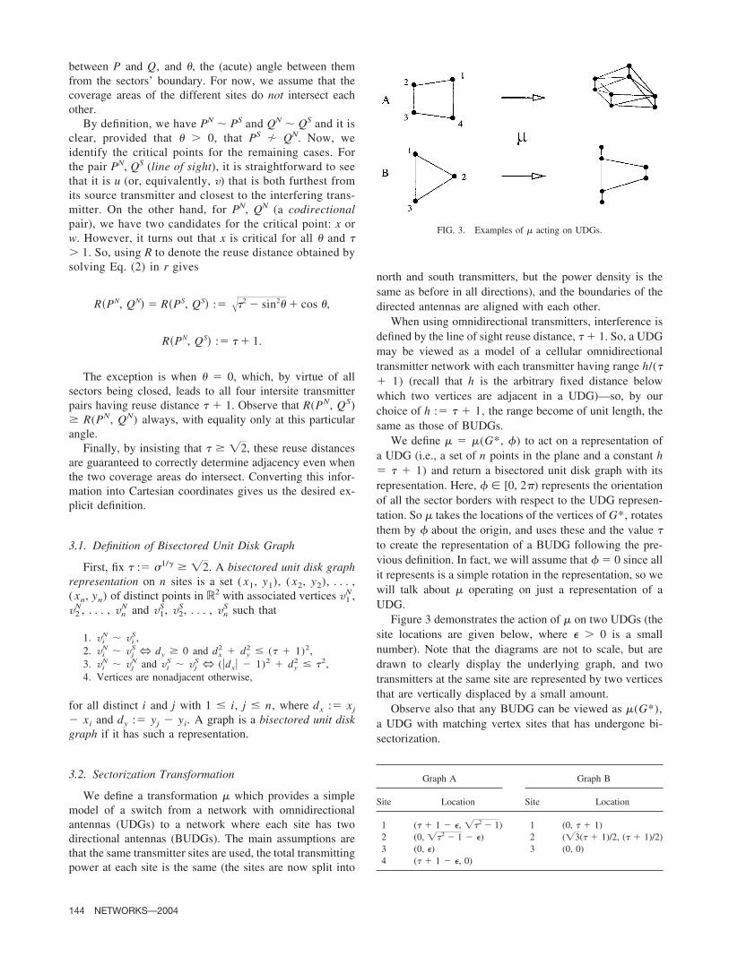
Figure 3 demonstrates the action of � on two UDGs (thesite locations are given below, where � � 0 is a smallnumber). Note that the diagrams are not to scale, but aredrawn to clearly display the underlying graph, and twotransmitters at the same site are represented by two verticesthat are vertically displaced by a small amount.

Observe also that any BUDG can be viewed as �(G*),a UDG with matching vertex sites that has undergone bi-sectorization.

Graph A Graph B

Site Location Site Location

1 (� � 1 � �, ��2 � 1) 1 (0, � � 1)2 (0, ��2 � 1 � �) 2 (�3(� � 1)/2, (� � 1)/2)3 (0, �) 3 (0, 0)4 (� � 1 � �, 0)

FIG. 3. Examples of � acting on UDGs.

144 NETWORKS—2004

3.3. Motivation

We are transforming a network with one (original) trans-mitter at each site into a network with two directionaltransmitters at each site. Since each transmitter has a limitedcapacity on its channel, if demand is sufficient, then bisec-torization could potentially double the number of users ofthe network, a significant improvement. This is done with-out the expensive procurement of new transmitter sites.

Recall that the chromatic number, �, represents the few-est number of channels necessary to guarantee acceptableinterference levels everywhere. Because the reuse distancesin �(G*) are no greater than that used in G*, we can“double up” any coloring of G* into a coloring of �(G*)using two disjoint color sets in the natural way. So, usingdouble the number of available channels in the new, bisec-tored network will always be sufficient [i.e., �(�(G*))� 2�(G*)]. However, we hope to be able to use as few aspossible, so that bisectorization significantly improves thecapacity-to-channel ratio of the network.

4. ELEMENTARY PROPERTIES OF BUDGs

Here, we discuss classification of BUDGs, some elemen-tary properties that we can tell about �(G*) given a UDGG*, and the maximum degree of a vertex in a BUDG.Although the definition of a BUDG is dependent on thevalue �, all these results hold for any � � �2 unlessotherwise stated.

4.1. Classification of BUDGs

It is not clear if BUDGs belong to any well-known classof graphs. They are certainly not perfect in general: The firstexample in Figure 3 is a BUDG that contains a copy of C5

as an induced subgraph. Like UDGs, BUDGs are not closedunder any edge operation (addition, deletion, contraction) orunder taking complements.

It is obvious that not all UDGs are BUDGs, for example,take any UDG which has isolated vertices or that has an oddnumber of vertices. Even excluding these simple counter-examples, the graph C4 is a UDG but not a BUDG (Fig. 4shows all possible BUDGs on two sites, i.e., four vertices).We now show the converse: that the class of BUDGs is notcontained in the class of UDGs. The first lemma is a resultthat was observed in [1, 8].

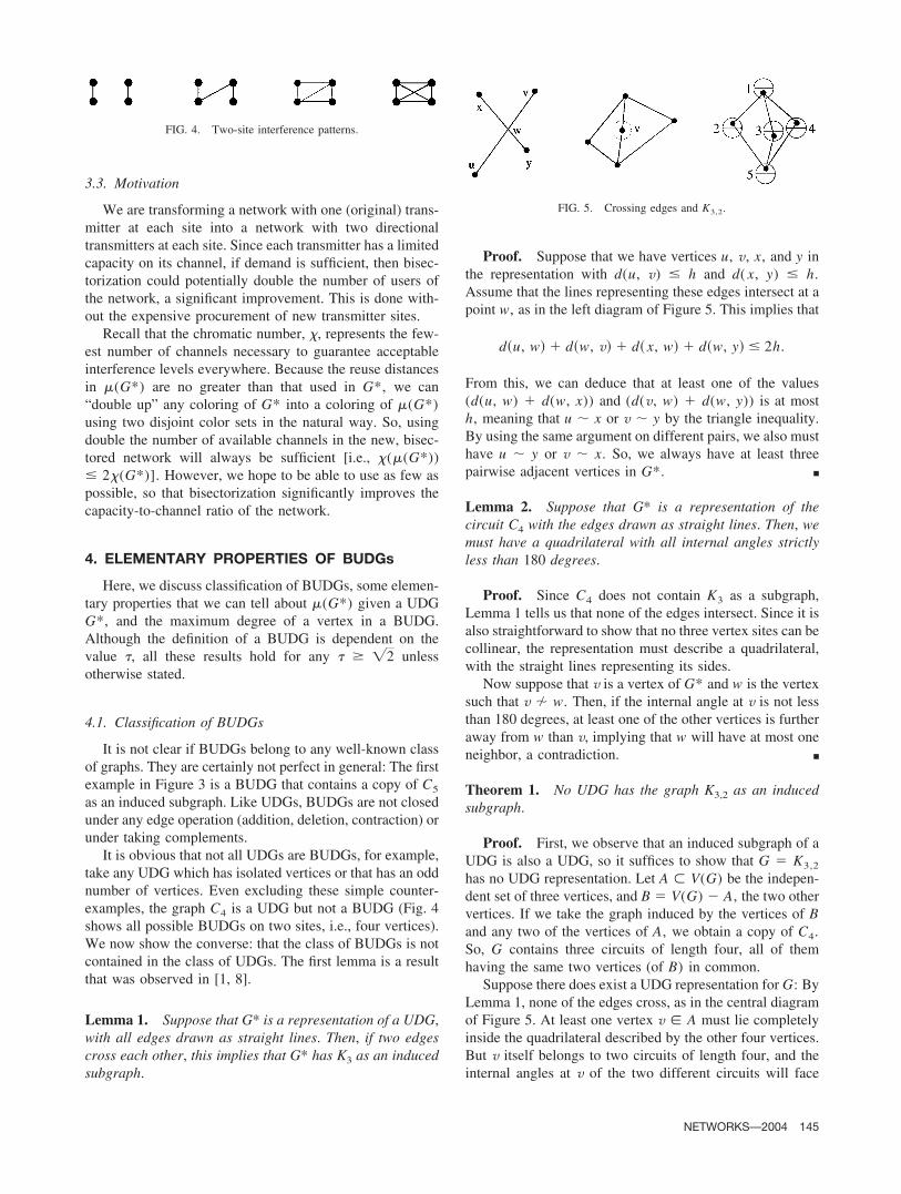
Lemma 1. Suppose that G* is a representation of a UDG,with all edges drawn as straight lines. Then, if two edgescross each other, this implies that G* has K3 as an inducedsubgraph.

Proof. Suppose that we have vertices u, v, x, and y inthe representation with d(u, v) � h and d( x, y) � h.Assume that the lines representing these edges intersect at apoint w, as in the left diagram of Figure 5. This implies that

du, w � dw, v � d x, w � dw, y � 2h.

From this, we can deduce that at least one of the values(d(u, w) � d(w, x)) and (d(v, w) � d(w, y)) is at mosth, meaning that u � x or v � y by the triangle inequality.By using the same argument on different pairs, we also musthave u � y or v � x. So, we always have at least threepairwise adjacent vertices in G*. ■

Lemma 2. Suppose that G* is a representation of thecircuit C4 with the edges drawn as straight lines. Then, wemust have a quadrilateral with all internal angles strictlyless than 180 degrees.

Proof. Since C4 does not contain K3 as a subgraph,Lemma 1 tells us that none of the edges intersect. Since it isalso straightforward to show that no three vertex sites can becollinear, the representation must describe a quadrilateral,with the straight lines representing its sides.

Now suppose that v is a vertex of G* and w is the vertexsuch that v � w. Then, if the internal angle at v is not lessthan 180 degrees, at least one of the other vertices is furtheraway from w than v, implying that w will have at most oneneighbor, a contradiction. ■

Theorem 1. No UDG has the graph K3,2 as an inducedsubgraph.

Proof. First, we observe that an induced subgraph of aUDG is also a UDG, so it suffices to show that G � K3,2

has no UDG representation. Let A � V(G) be the indepen-dent set of three vertices, and B � V(G) � A, the two othervertices. If we take the graph induced by the vertices of Band any two of the vertices of A, we obtain a copy of C4.So, G contains three circuits of length four, all of themhaving the same two vertices (of B) in common.

Suppose there does exist a UDG representation for G: ByLemma 1, none of the edges cross, as in the central diagramof Figure 5. At least one vertex v � A must lie completelyinside the quadrilateral described by the other four vertices.But v itself belongs to two circuits of length four, and theinternal angles at v of the two different circuits will face

FIG. 4. Two-site interference patterns.

FIG. 5. Crossing edges and K3,2.

NETWORKS—2004 145

different directions and yet must add up to 360 degrees.However, this contradicts the fact from Lemma 2 that allinternal angles must be less than 180 degrees. ■

Corollary 1. There exist BUDGs that are not UDGs.

Let � � min(�, �3(� � 1)/2) and � �� �, where � and� are small positive numbers. Consider the BUDG createdby having transmitter sites at the following points:

Site Location

1 (0, � � �)2 (�((� � 1)/2) � �, 0)3 (1, ��)4 (((� � 1)/2) � �, 0)5 (0, �(3�2/4) � (�/2) � 1/4)(1/2) � �)

Then, by taking the induced graph of the north-facingvertices at sites 2, 4, and 5 and the south facing vertices atsites 1 and 3, it can be shown that K3,2 is the inducedsubgraph, as shown in the final diagram of Figure 5. ■

4.2. Clique Number

The clique number itself provides a natural lower boundon the chromatic number of a graph and will be used lateralso to help construct upper bounds on the chromatic num-ber. The value �(�(G*)) may be higher or lower than�(G*), depending on G* (Fig. 3 demonstrates both thesecases). For any G*, we always have

��G* � 2�G*. (3)

To see this, let U � V(�(G*)) be the vertices of a maxi-mum clique in the bisectored graph. We know from thedefinition that the sites of any two vertices in U must bewithin distance � � 1. Now consider ��1(U): defined to bethe vertices of G* that correspond to the sites of the trans-mitters in U—there must be at least �(�(G*))/ 2 of them,and since they are all within distance � � 1, they form aclique in G*. The result follows.

(3) is tight, as we can define Gk to be the UDG whosevertices lie at the points (1/k, 0), (2/k, 0), . . . (k/k, 0).Then, �(Gk) � k, and because the angle � between allvertex sites in �(Gk) is zero, all pairs of vertices areadjacent in �(Gk), and so �(�(Gk)) � 2k.

Let us suppose that the angle � 0 for any pair ofvertices—in other words, different transmitter sites havedistinct y-coordinates in �(G*) (and, therefore, in G*). LetU � V(�(G*)) be the vertices of a clique, as before. Then,at most one site can contain two vertices (transmitters) of U;otherwise, there would be a nonadjacent pair (as with PS,QN in Fig. 2). So, after considering ��1(U), we have

��G* � �G* � 1. (4)

In some ways, this model with sites always having distincty-coordinates is more realistic, so this result implies that �is likely to force at most a small increase in the cliquenumber.

Often, the nature of real cellular networks is such that acoloring of the maximum clique of a graph can be extendedto the whole graph with no or few additional colors (e.g., see[6]). This implies that the chromatic number is usually closeor equal to the clique number. Equation (4) therefore sug-gests that we will not need much extra spectrum followingbisectorization.

4.3. Chromatic Number

The chromatic number can also go up or down as a resultof �. Figure 3(B) shows an instance where �(G*) � 3 but�(�(G*)) � 2. As mentioned before, for any G*, wealways have �(�(G*)) � 2�(G*). However, in contrast tothe clique number, Figure 3(A) shows a construction prov-ing that this bound is tight which does not use zero-degreeangles between sites [here, we have �(G*) � 2 and�(�(G*)) � 4]. However, it is unknown whether thisbound is tight in general. Our main bounds concerning thechromatic number are discussed in the next section.

4.4. Maximum Degree

It is straightforward to see that the maximum degree of abisectored graph, �(�(G*)), can be bounded by �(�(G*))� 2�(G*) � 1, but we aim to find a bound of the form�(�(G*)) � c � �(�(G*)), where c is a constant. Al-though � is not directly useful to us, the methods describedhere will be used later for bounds on the chromatic number.

Let G* be a representation of a unit disk graph, and letp � ( px, py) be an arbitrary point on the plane. Define Dp

to be the closed disk of radius (� � 1)/2 with center at pointp.

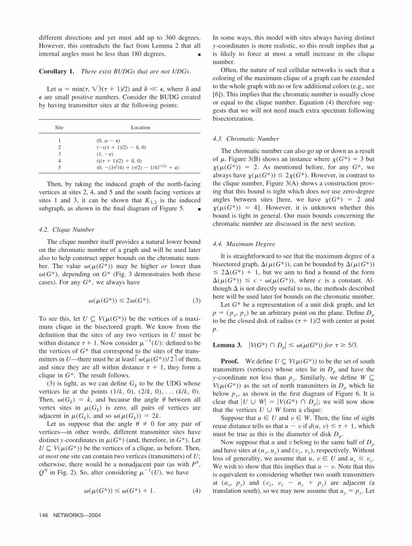
Lemma 3. �V(G*) � Dp� � �(�(G*)) for � � 5/3.

Proof. We define U � V(�(G*)) to be the set of southtransmitters (vertices) whose sites lie in Dp and have they-coordinate not less than py. Similarly, we define W �V(�(G*)) as the set of north transmitters in Dp which liebelow py, as shown in the first diagram of Figure 6. It isclear that �U � W� � �V(G*) � Dp�; we will now showthat the vertices U � W form a clique:

Suppose that u � U and v � W. Then, the line of sightreuse distance tells us that u � v if d(u, v) � � � 1, whichmust be true as this is the diameter of disk Dp.

Now suppose that u and v belong to the same half of Dp

and have sites at (ux, uy) and (vx, vy), respectively. Withoutloss of generality, we assume that u, v � U and uy � vy.We wish to show that this implies that u � v. Note that thisis equivalent to considering whether two south transmittersat (ux, py) and (vx, vy � uy � py) are adjacent (atranslation south), so we may now assume that uy � py. Let

146 NETWORKS—2004

X :� {(ux � 1, py), (ux � 1, py)}. These points lie in thebroadcast area of and at distance 1 from transmitter u. Theyalso lie in the angular range of v, so if we can show that d(v,x) � � for an x � X then the two transmitters are adjacent.Define dX(v) :� minx�Xd(v, x). There are two cases toconsider:

1. There is an x � X such that d( x, p) � [(� � 1)/ 2] �1. Then, it follows by the triangle inequality that d(v, x)� d(v, p) � d( p, x) � ((� � 1)/ 2) � (((� � 1)/ 2)� 1) � �, as required.

2. Otherwise, we have ux � 1 � px � ((� � 1)/ 2) � 1and ux � 1 � px � ((� � 1)/ 2) � 1. Rearranginggives px � ((3 � �)/ 2) � ux � px � ((3 � �)/ 2),implying that both � � 3 and px � 1 � ux � px � 1in this case. If vx � ux � 1 or vx � ux � 1, then,clearly, dX(v) � d(v, p) � ((� � 1)/ 2) � �.

Finally, we assume that ux � 1 � vx � ux � 1. Then,dX(v) is maximized when ux � px and v � ( px, py � ((�� 1)/ 2)). So, dx(v)2 � ((� � 1)/ 2)2 � 12 � �2 for� � 5/3. ■

Theorem 2. �(�(G*)) � 11�(�(G*)) � 1 for � � 5/3.

Proof. Without loss of generality, let u represent anorth sector in �(G*). Let �u be a closed disk of radius �� 1 centered at the site of u. Then, all vertices adjacent tou must have sites lying in �u: We now find an upper boundfor this value.

We partition �u into areas A1, . . . , A7. First, let A1 tobe the closed disk of radius (� � 1)/2 at u. We then dividethe rest of �u into six equally sized segments, A2, . . . , A7,as demonstrated in the center diagram of Figure 6. Theangle ranges of these six sectors (from the reference angleshown in the same diagram) are [0, /3], ( /3, 2 /3), [2 /3, ], ( , 4 /3), [4 /3, 5 /3], and (5 /3, 0), respectively(deliberately chosen so that all points in A5, A6, and A7

have lower y-coordinate than p).Let D1, . . . , D7 be closed disks of radius (� � 1)/2

centered at the points p1, . . . , p7 as given in the tablebelow and shown in the last diagram of Figure 6:

Point Location

p1: (0, 0)

p2: (3

4(� � 1), �3

4(� � 1))

p3: (0, �3

2(� � 1))

p4: (� 3

4(� � 1), �3

4(� � 1))

p5: (� 3

4(� � 1), � �3

4(� � 1))

p6: (0, � �3

2(� � 1))

p7: (3

4(� � 1), � �3

4(� � 1))

This gives us Ai � Di, for 1 � i � 7. By Lemma 3,each Ai contains at most � � �(�(G*)) transmitter sites.In A5, A6, and A7, no south transmitters are adjacent to u,so each contribute at most � neighbors to u. In A2, A3, andA4, each site may contribute up to two neighbors (both thenorth and the south transmitters) to u. In A1 also, each sitemay contribute two except for the site of u itself, whichprovides exactly one neighbor. Hence,

��G* � 3� � 3 � 2� � 2� � 1 � 11� � 1. ■

5. COLORING BUDGs

Colorings of BUDGs are the most important feature fromour perspective, as they coincide with channel assignmentswith acceptable interference levels everywhere. We will dis-cuss some upper bounds on the chromatic number and mentioncorresponding approximation and coloring algorithms whereappropriate. For clarity, we will use the notation B* � �(G*)to represent a BUDG with its representation.

First, we mention that determining 3-colorability is anNP-complete problem for BUDGs† with � � 2, implyingthat finding � is NP-Hard for such graphs. This provides ourmotivation for finding approximations to the chromaticnumber. Two straightforward bounds are

† The fact that determining 3-colorability for BUDGs is NP-Hard can beproved using a transformation from the problem of 3-colorability for generalgraphs. The proof runs similar to that described in [5] for UDGs, although theconstruction is a little more involved and does not work if � � 2.

FIG. 6. Constructions for Lemma 3 and Theorem 2.

NETWORKS—2004 147

1. �(B*) � 6�(G*) � 4. This follows from Peeters’result for UDGs and the observation that �(B*)� 2�(G*). Finding such a coloring is possible in poly-nomial time simply by finding the corresponding UDGcoloring and applying it to the north and south transmit-ters separately using disjoint color sets.

2. �(B*) � 11�(B*), which follows directly from Theo-rem 2.

However, in a way similar to the derivation of Peeters’result, a lexicographical ordering can be used to reduce thelatter bound further.

Let � be an ordering v1, v2, . . . , vn on the vertices ofB*. Define the preneighborhood of a vertex vi (with respectto �) and the degree of � to be

��vi :� Nvi � �vj� j � i�,

�� :� max1�i�n

���vi�,

respectively. Consider applying the greedy coloring algo-rithm to the vertices: We take them in ascending order,assigning each one the lowest color (using � as the colorset) that is not used by any of its preneighbors. In the worstcase, all a vertex’s preneighbors will have different colors,so it follows that

�B* � �� � 1 � �B* � 1, for all �. (5)

Theorem 3. �(B*) � 7�(B*) � 1 for � � 5/3.

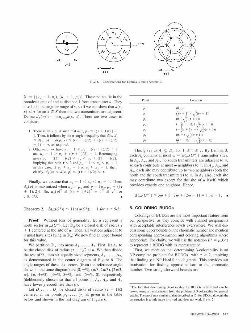
Proof. We will use the lexicographical ordering �defined as follows: For u and v two distinct vertices of B*,

u � v N �uy � �3ux � vy � �3vx, oruy � �3ux � vy � �3vx and uy � vy, orux � vx, uy � vy and u is a south vertex.

We now bound ��. Suppose, first, that v is a north trans-mitter, as in the first diagram of Figure 7. Then, followingthe area definitions of Figure 6, areas A2, A3, and A7 will

contain no preneighbors of v by virtue of the ordering. ByLemma 3, the remaining areas contain at most �(B*) trans-mitter sites each. So, A4 contributes at most 2�(B*) neigh-bors, while A5 and A6 contribute at most �(B*), due to thefact that their south transmitters will be nonadjacent to v.Finally, A1 may also contribute up to 2�(B*), but we canexclude v itself. Hence,

���v� � 6�B* � 1.

Now, take v to be a south transmitter. The analysis issimilar, but note that it is area A4 that contributes at most�(B*) neighbors, while A5 and A6 can provide at mostdouble this amount. For A1, we can exclude v and itscorresponding north transmitter as potential preneighbors.So,

���v� � 7�B* � 2,

which gives us an upper bound on ��, and, therefore, theresult by (5). ■

Corollary 2. Let B be a bisectored unit disk graph for �� 5/3 without its representation. Then, B can be coloredwith at most 7�(B) � 1 colors in O(�V(B)�2) time.

Proof. It was shown in [9] how we can find a mini-mum-degree ordering (known as the smallest-last ordering)of the vertices for any graph G in time O(�V(G) � E(G)�).Since the degree of this ordering must be at most ��, thebound on the number of colors follows from Theorem 3. Itfollows that this ordering can be found and the greedycoloring algorithm applied in time O(�V(B)� � �E(B)�)� O(�V(B)� � ��(B)�) � O(�V(B)2�). ■

A different approach to the problem is to consider divid-ing the graph up into subgraphs whose chromatic numbercan be solved easily. Recall that a co-comparability graph isperfect and an optimum coloring can be found in polyno-mial time using, for example, Mohring’s algorithm [11].

FIG. 7. Potential preneighbors of north and south transmitters under �.

148 NETWORKS—2004

The technique of dividing UDGs into “strips” that areco-comparable graphs is well known (see, e.g., [1, 5, 8]).

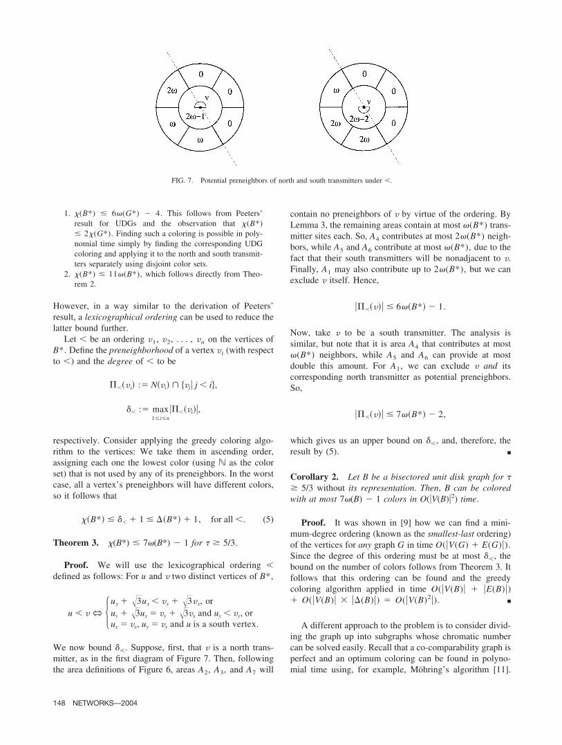
We define a t-strip BUDG to be BUDG which has arepresentation B* such that, for all u, v � B*, �vx � ux� �t. The first diagram in Figure 8 demonstrates this.

Lemma 4. Let B* be a �2� � 1-strip BUDG. Then, B* isa co-comparability graph.

Proof. We will define an orientation on nonadjacentvertex pairs according to the y-coordinates of their vertexsites: For all u and v in V(B*), we say that u � v if andonly if u � v and uy � vy. (Note that, due to the width ofB*, it is not possible for vertices with the same y-coordinateto be nonadjacent.) We will show that � is transitive and,hence, prove co-comparability.

So, let us assume that u, v, and w are vertices in B*, withu � v and v � w. Define x :� �2� � 1, the maximumhorizontal distance between sites, and let h1 :� vy � uy, h2

:� wy � vy, and h :� h1 � h2 � wy � uy. Weautomatically have wy � uy: We must prove that nonadja-cency holds. Since each vertex can represent a north or asouth transmitter, there are (excluding symmetries) fourcases to consider, the first three of which are shown inFigure 8:

1. u and w are north, v is south.For u and v to be nonadjacent, we need the distance

between their sites to be greater than � � 1. Hence, h12 �

(� � 1)2 � x2 � �2, from which we have h � �,implying that u � w.

2. u and v are north, w is south.Following the same argument, the distance between v

and w must be greater than � � 1; hence, h2 � �.However, here, we need h � � � 1 to prove that u � w,so we must show h1 � 1.

For u and v to be nonadjacent, it must be true that thedistance from site u to the corner of the semicircle of therange of v closest to u is greater than �. So, we must haveh1

2 � �2 � ( x � 1)2, from which

h12 � �2 � 2� � 2�2� � 1 � 2 � 1, @� � �2.

3. u, v and w are all north.As with h1 from the previous case, here both h1

2 and

h22 are greater than �2 � ( x � 1)2, so h2 � 4�2 � 4( x

� 1)2. Expanding gives

h2 � 4�2 � 8� � 8�2� � 1 � 8 � �2 @� � �2.

This gives us h � � and, therefore, u � w.4. u is south and w is north.

Then, since wy � uy, we know immediately that u �w as the two vertices represent sectors that face oppositedirections. ■

Remark. The direction of the strips is important. If thestrips ran parallel to the sector borders, instead of perpen-dicular to them (i.e., the criterion was �vy � uy� � t), thenonly strip BUDGs of width zero would necessarily beco-comparability graphs.

Theorem 4. Let B* be a BUDG. Then,

�B* � � � � 1

�2� � 1� 1� � �B*.

Proof. Let t � �2� � 1 and u be a transmitter sitewith lowest horizontal coordinate. We define Sk (k � � �{0}) to be the t-strip BUDG obtained by taking the inducedsubgraph of the vertices lying in the horizontal range [ux

� kt, ux � (k � 1)t) in the representation of B*.Each Sk is perfect (a consequence of Lemma 4) and,

hence, colorable with at most �(Sk) � �(B*) colors.Consider �k � �n���{0} Sk�in, for i a fixed integer and0 � k � i: If i is large enough, then two sites in �k thatbelong to different strips will always be at least distance �� 1 apart, so a coloring of �k will always be extendable toa coloring of B*. This happens when i � (� � 1)/t � 1.So, using disjoint color sets to color each �k gives us acomplete coloring of B* using the required number ofcolors. ■

Combining this result with Mohring’s algorithm allowsus to find a coloring in polynomial time which has a rela-tively good bound when � is low and works for all � � �2.However, we do require the representation of the BUDG inorder to implement this algorithm.

FIG. 8. A t-strip BUDG and the three cases of Lemma 4.

NETWORKS—2004 149

6. EXPERIMENTAL RESULTS

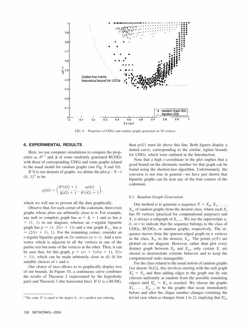
Here, we use computer simulations to compare the prop-erties �, �* ‡ and � of some randomly generated BUDGswith those of corresponding UDGs and some graphs relatedto the usual model for random graphs (see Fig. 9 and 10).

If � is our domain of graphs, we define the plot p : � 3(0, 1]2 to be

pG � ��*G � 1

�G � 1,

�G

�*G � 1� ,

which we will use to present all the data graphically.Observe that, for each corner of the codomain, there exist

graphs whose plots are arbitrarily close to it. For example,any null or complete graph has � � � � 1 and so has p� (1, 1) in our diagram, whereas an r-regular bipartitegraph has p � (1, 2/(r � 1)) and a star graph K1,r has p� (2/(r � 1), 1). For the remaining corner, consider anr-regular bipartite graph on 2n vertices (n � r). Add a newvertex which is adjacent to all the vertices in one of thepartite sets but none of the vertices in the other. Then, it canbe seen that, for this graph, p � ((r � 1)/(n � 1), 2/(r� 1)), which can be made arbitrarily close to (0, 0) forsuitable choices of r and n.

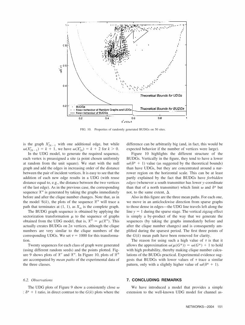
Our choice of axes allows us to graphically display twoof our bounds. In Figure 10, a continuous curve combinesthe results of Theorem 2 (represented by the hyperbolicpart) and Theorem 3 (the horizontal line): If G is a BUDG,

then p(G) must lie above this line. Both figures display adotted curve, corresponding to the similar, tighter boundsfor UDGs, which were outlined in the Introduction.

Note that a high y-coordinate in the plot implies that agood bound on the chromatic number for that graph can befound using the shortest-last algorithm. Unfortunately, theconverse is not true in general—we have just shown thatbipartite graphs can lie near any of the four corners of thecodomain.

6.1. Random Graph Generation

Our method is to generate a sequence � � X0, X1, . . . ,Xm of random graphs from the desired class, where each Xi

has 50 vertices (practical for computational purposes) andXi is always a subgraph of Xi�1. We use the superscripts u,b, or r to indicate that the sequence belongs to the class ofUDGs, BUDGs, or random graphs, respectively. The se-quence moves from the sparsest-edged graph on n verticesin the class, X0, to the densest, Xm. The points p(�) areplotted on our diagram. However, rather than plot everydistinct graph between X0 and Xm, only certain Xi arechosen to demonstrate extreme behavior and to keep thecomputational tasks manageable.

For the class related to the usual notion of random graphs[we denote �(k)], this involves starting with the null graphX0

r � Nn and then adding edges to the graph one by one(chosen uniformly at random from the possible remainingedges) until Xm

r � Kn is reached. We choose the graphsX1

r , . . . , Xm�1r to be the graphs that occur immediately

before and after the clique number changes (omitting thetrivial case when � changes from 1 to 2), implying that X2k

r‡ The value �* is equal to the degree �� of a smallest last ordering.

FIG. 9. Properties of UDGs and random graphs generated on 50 vertices.

150 NETWORKS—2004

is the graph X2k�1r with one additional edge, but while

�(X2k�1r ) � k � 1, we have �(X2k

r ) � k � 2 for k � 0.In the UDG model, to generate the required sequence,

each vertex is preassigned a site (a point chosen uniformlyat random from the unit square). We start with the nullgraph and add the edges in increasing order of the distancebetween the pair of incident vertices. It is easy to see that theaddition of each new edge results in a UDG (with reusedistance equal to, e.g., the distance between the two verticesof the last edge). As in the previous case, the correspondingsequence �u is generated by taking the graphs immediatelybefore and after the clique number changes. Note that, as inthe model �(k), the plots of the sequence �u will trace apath that terminates at (1, 1), as Xm is the complete graph.

The BUDG graph sequence is obtained by applying thesectorization transformation � to the sequence of graphsobtained from the UDG model, that is, �b � �(�u). Thisactually creates BUDGs on 2n vertices, although the cliquenumbers are very similar to the clique numbers of thecorresponding UDGs. We set � � 1000 for this transforma-tion.

Twenty sequences for each class of graph were generated(using different random seeds) and the points plotted. Fig-ure 9 shows plots of �r and �u. In Figure 10, plots of �b

are accompanied by mean paths of the experimental data ofthe three classes.

6.2. Observations

The UDG plots of Figure 9 show a consistently close �: �* � 1 ratio, in direct contrast to the G(k) plots where the

difference can be arbitrarily big (and, in fact, this would beexpected behavior if the number of vertices were large).

Figure 10 highlights the different structure of theBUDGs. Vertically in the figure, they tend to have a lower�/(�* � 1) value (as suggested by the theoretical bounds)than have UDGs, but they are concentrated around a nar-rower region on the horizontal scale. This can be at leastpartly explained by the fact that BUDGs have forbiddenedges (whenever a south transmitter has lower y-coordinatethan that of a north transmitter) which limit � and �* butnot, to the same extent, �.

Also in this figure are the three mean paths. For each one,we move in an anticlockwise direction from sparse graphsto those dense in edges—the UDG line travels left along theline y � 1 during the sparse stage. The vertical zigzag effectis simply a by-product of the way that we generate thesequences (by taking the graphs immediately before andafter the clique number changes) and is consequently am-plified during the sparsest period. The first three points ofthe G(k) mean path have been removed for clarity.

The reason for using such a high value of � is that itallows the approximation �(�(G*)) � �(G*) � 1 to holdwith high probability, thereby making clique number calcu-lations of the BUDGs practical. Experimental evidence sug-gests that BUDGs with lower values of � trace a similarpattern, only with a slightly higher value of �/(�* � 1).

7. CONCLUDING REMARKS

We have introduced a model that provides a simpleextension to the well-known UDG model for channel as-

FIG. 10. Properties of randomly generated BUDGs on 50 sites.

NETWORKS—2004 151

signment, to allow for the phenomenon of cell sectorization.We focused on the chromatic number, which equals thesmallest amount of spectrum necessary for a satisfactoryservice. Theorems 3 and 4 provide upper bounds in terms ofthe clique number and can be loosely regarded as measuresof the relative difficulty in finding a good solution forBUDGs.

We do not claim that the bounds on � and �* for BUDGsare tight: Rather, they are in some ways intuitive boundsthat give a reasonable approximation. Tight bounds arelikely to depend explicitly on �.

A further unknown is whether the clique number ofBUDGs can be calculated in polynomial time. Many of theresults concerning BUDGs mirror similar results concerningUDGs, so the expected answer is yes. A final, more general,question is whether there are any qualitative differences toobserve if the restriction on aligning the sectors is removedand/or we consider k-sectored unit disk graphs where k� 2.

REFERENCES

[1] H. Breu, Algorithmic aspects of constrained unit diskgraphs, Ph.D. Thesis, University of British Columbia, 1996.

[2] H. Breu and D.G. Kirkpatrick, Unit disk graph recognitionis NP-hard, Comput Geom Theory Appl 9(1–2) (1998),3–24.

[3] B.N. Clark, C.J. Colbourn, and D.S. Johnson, Unit diskgraphs, Discr Math 86 (1990), 165–177.

[4] M.R. Garey and D.S. Johnson, Computers and intractability,W.H. Freeman, New York, 1979.

[5] A. Graf, M. Stumpf, and G. Weissenfels, On coloring unitdisk graphs, Algorithmica 20 (1998), 288–293.

[6] S. Hurley, D.H. Smith, and S.U. Thiel, FASoft: A systemfor discrete channel frequency assignment, Radio Sci 32(1997), 1921–1939.

[7] L. Lovasz, “Perfect graphs,” Selected topics in graph the-ory, L.W. Beineke and R.J. Wilson (Editors), AcademicPress, New York, 1983, Vol. 2, Chapter 3.

[8] E. Malesinska, S. Piskorz, and G. Weissenfels, On thechromatic number of disk graphs, Networks 32 (1998),13–22.

[9] D.W. Matula and L.L. Beck, Smallest-last ordering andclustering and graph coloring algorithms, J Assoc ComputMachin 30 (1983), 417–427.

[10] T.S. Michael and T. Quint, Sphere of influence graphs: Asurvey, Congress Num 105 (1994), 153–160.

[11] R.H. Mohring, “Algorithmic aspects of comparabilitygraphs and interval graphs,” Graphs and orders, I. Rival(Editor), D. Reidel, Boston, 1985, pp. 41–101.

[12] J. Mycielski, Sur le coloriage des graphs, Colloq Math 3(1955), 161–162.

[13] R. Peeters, On coloring j-unit sphere graphs, Department ofEconomics, Tilburg University, Netherlands, 1991.

[14] V. Raghavan and J. Spinrad, Robust algorithms for re-stricted domains, Proc 12th Annual ACM–SIAM Symp onDiscrete Algorithms, ACM Press, Washington, DC, 2001,pp. 460–467.

152 NETWORKS—2004