Embed Size (px)
Citation preview
bivariate EDA and regression analysis
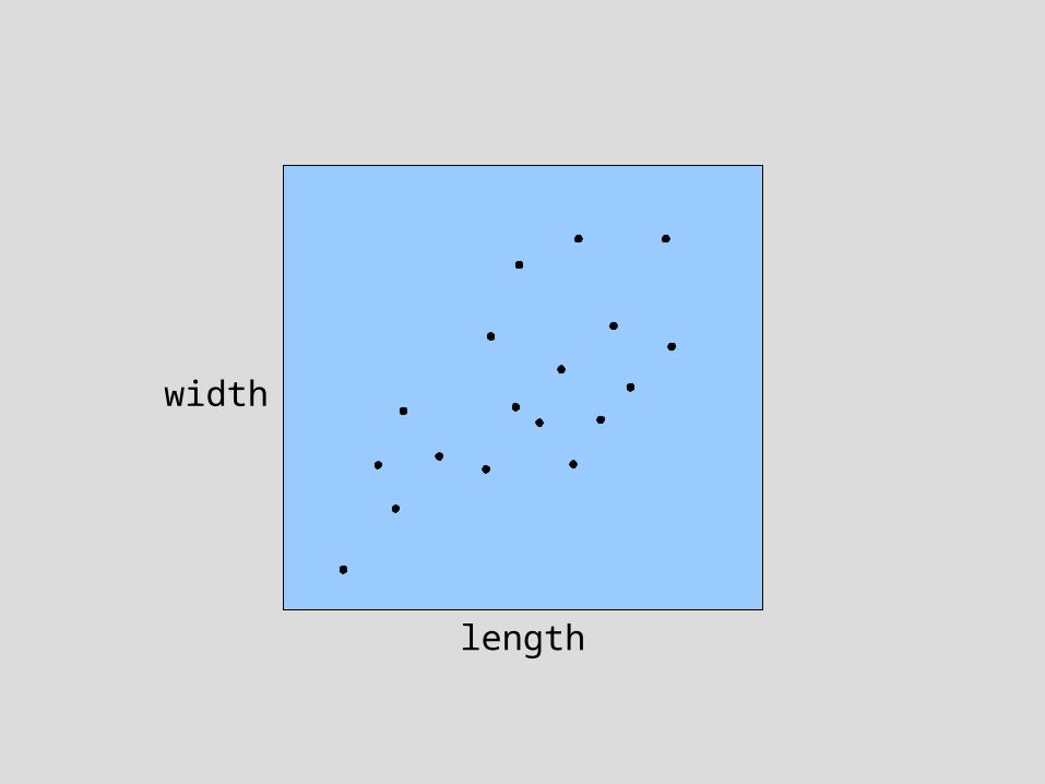
length
width
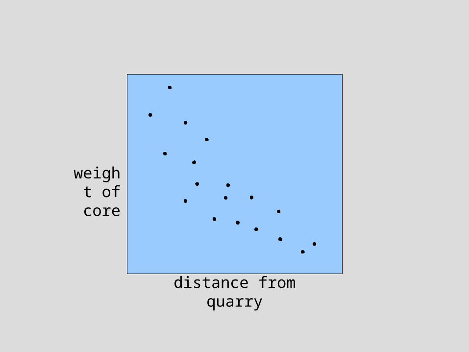
distance from quarry
weight of core
-4 -3 -2 -1 0 1 2 3 4 5AG_C1_1
-5
-4
-3
-2
-1
0
1
2
3
AG
_C1_
2
-4 -3 -2 -1 0 1 2 3 4 5AG_C1_1
-5
-4
-3
-2
-1
0
1
2
3
AG
_C
1_
2
-4 -3 -2 -1 0 1 2 3 4 5AG_C1_1
-5
-4
-3
-2
-1
0
1
2
3
AG
_C1_
2
AG_C1_2
AG
_C1_
1
AG_C2_2 AG_C3_2 AG_C4_2
AG
_C1_1
AG
_C2_
1A
G_C
2_1A
G_C
3_1
AG
_C3_1
AG_C1_2
AG
_C4_
1
AG_C2_2 AG_C3_2 AG_C4_2
AG
_C4_1
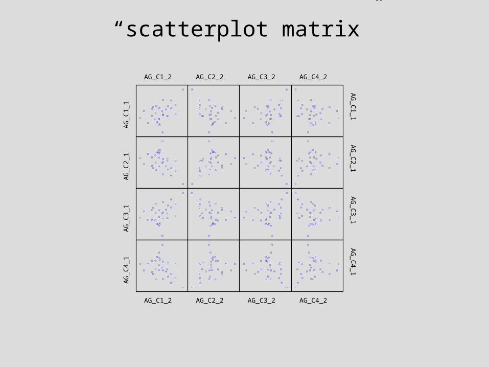
“scatterplot matrix”

AG_C1_1
AG
_C
1_
1
AG_C2_1 AG_C3_1 AG_C4_1 AG_C1_2 AG_C2_2 AG_C3_2 AG_C4_2
AG
_C
1_
1
AG
_C
2_
1 AG
_C
2_
1
AG
_C
3_
1 AG
_C
3_
1
AG
_C
4_
1 AG
_C
4_
1
AG
_C
1_
2 AG
_C
1_
2
AG
_C
2_
2 AG
_C
2_
2
AG
_C
3_
2 AG
_C
3_
2
AG_C1_1
AG
_C
4_
2
AG_C2_1 AG_C3_1 AG_C4_1 AG_C1_2 AG_C2_2 AG_C3_2 AG_C4_2
AG
_C
4_
2
-4 -3 -2 -1 0 1 2 3 4 5AG_C1_1
-10
-5
0
5
10
AG
_C2_
1
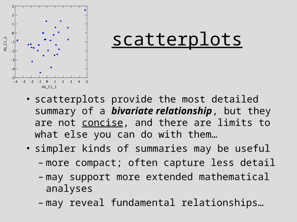
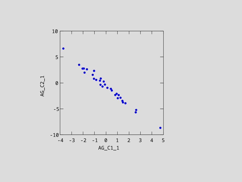
scatterplots
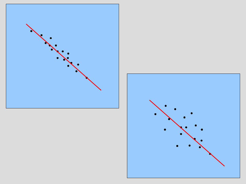
• scatterplots provide the most detailed summary of a bivariate relationship, but they are not concise, and there are limits to what else you can do with them…
• simpler kinds of summaries may be useful– more compact; often capture less detail– may support more extended mathematical analyses– may reveal fundamental relationships…
-4 -3 -2 -1 0 1 2 3 4 5AG_C1_1
-5
-4
-3
-2
-1
0
1
2
3A
G_
C1
_2
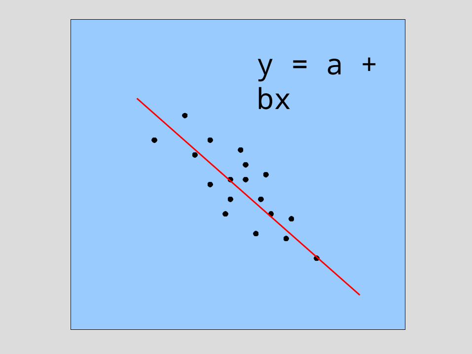
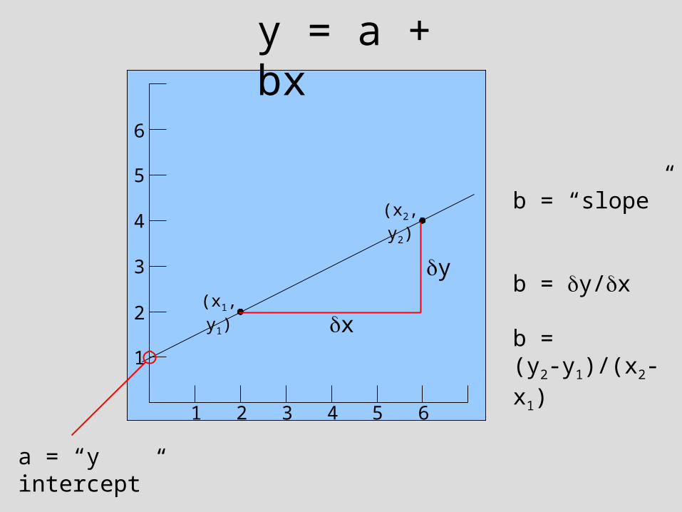
y = a + bx
y = a + bx
1 2 3 4 5 6
1
2
3
4
5
6
a = “y intercept”
y
x
(x2,y2)
(x1,y1)
b = “slope”
b = y/x
b = (y2-y1)/(x2-x1)
y = a + bx
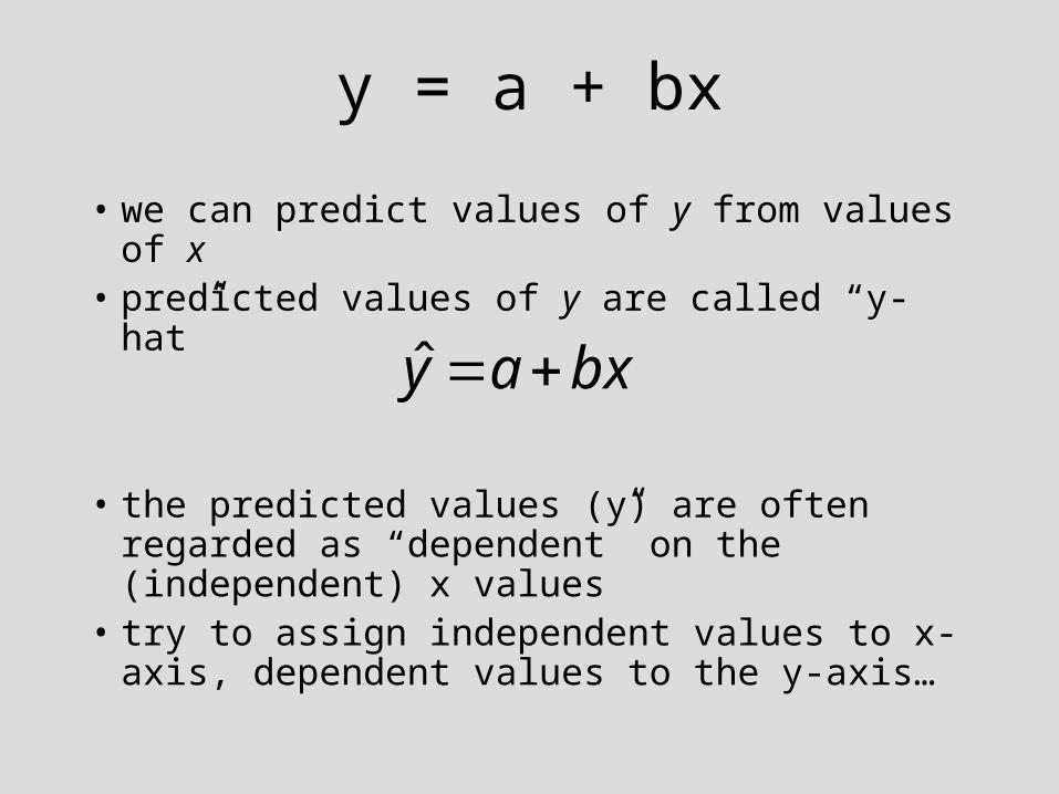
• we can predict values of y from values of x• predicted values of y are called “y-hat”
• the predicted values (y) are often regarded as “dependent” on the (independent) x values
• try to assign independent values to x-axis, dependent values to the y-axis…
bxay ˆ
y = a + bx
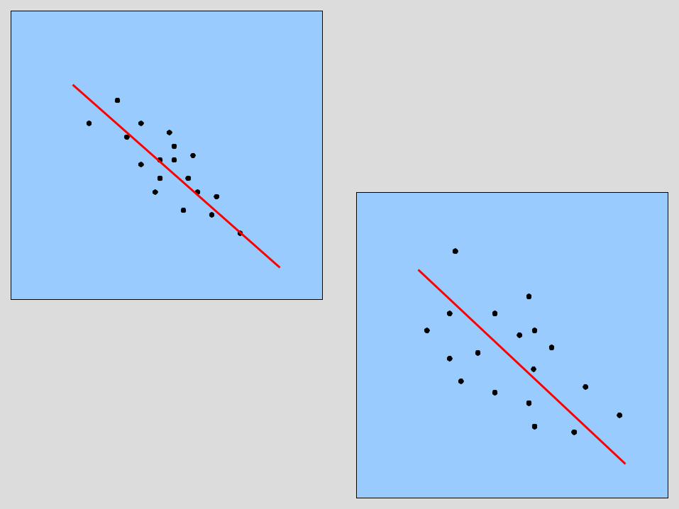
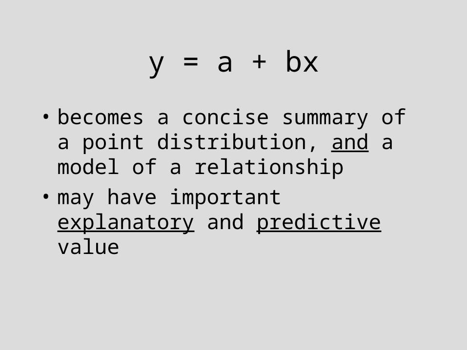
• becomes a concise summary of a point distribution, and a model of a relationship
• may have important explanatory and predictive value
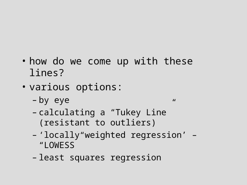
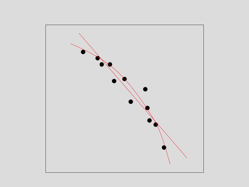
• how do we come up with these lines?
• various options:– by eye– calculating a “Tukey Line” (resistant to
outliers)– ‘locally weighted regression’ – “LOWESS”– least squares regression
linear regression
• linear regression and correlation analysis are generally concerned with fitting lines to real data
• least squares regression is one of the main tools
• attempts to minimize deviation of observed points from the regression line
• maximizes its potential for prediction
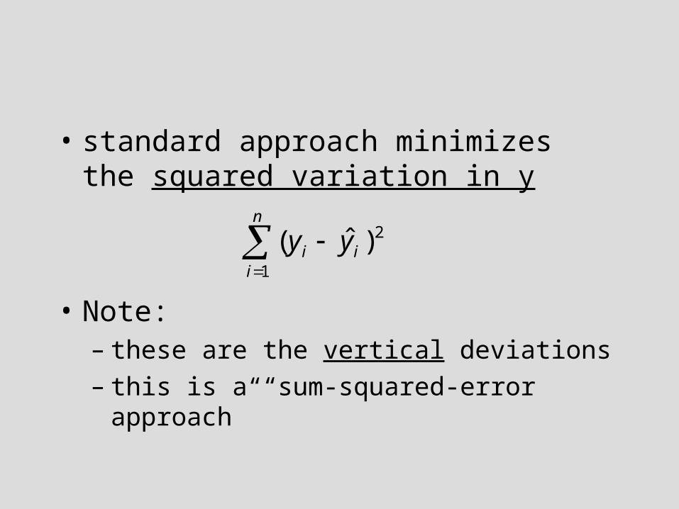
• standard approach minimizes the squared variation in y
• Note:– these are the vertical deviations– this is a “sum-squared-error approach”
n
iii yy
1
2)ˆ(
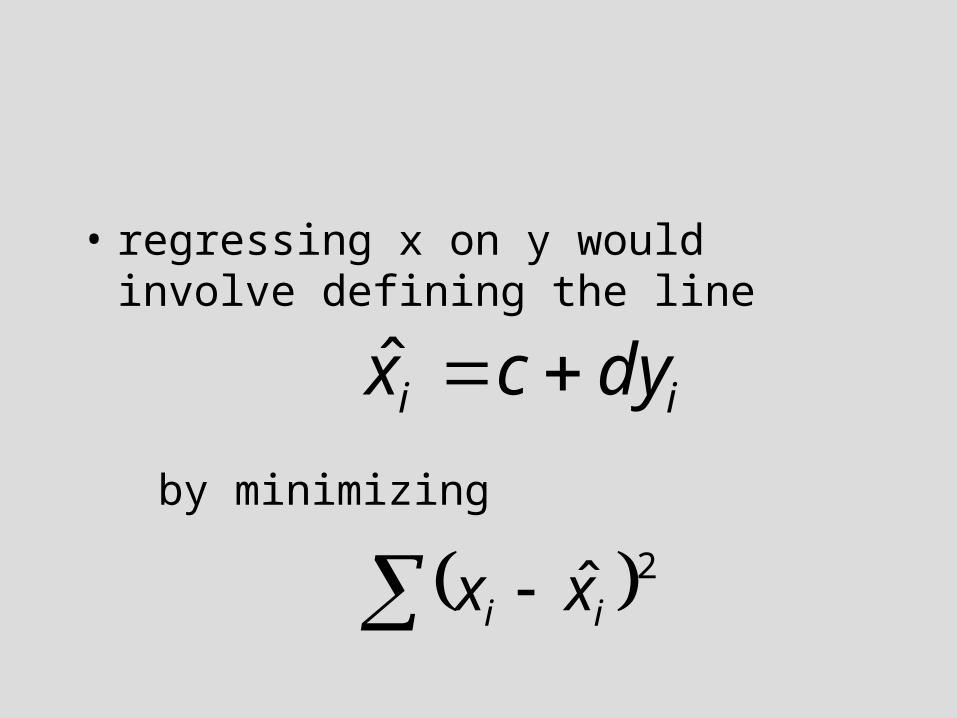
• regressing x on y would involve defining the line
by minimizing
ii dycx ˆ
2ˆii xx
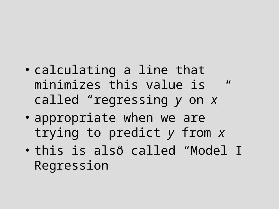
• calculating a line that minimizes this value is called “regressing y on x”
• appropriate when we are trying to predict y from x
• this is also called “Model I Regression”
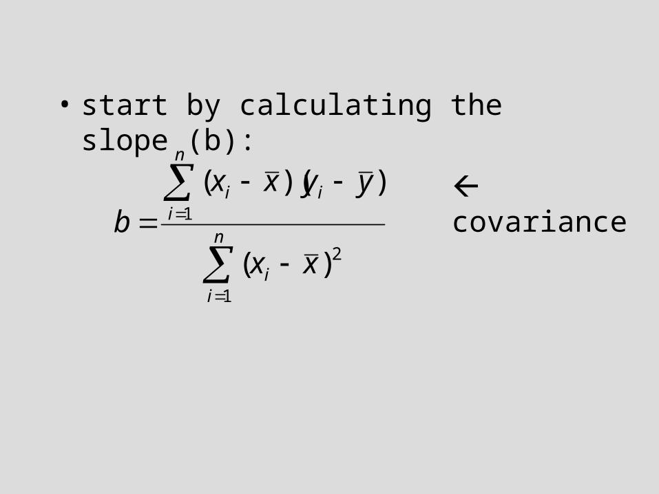
• start by calculating the slope (b):
n
ii
n
iii
xx
yyxxb
1
2
1
)(
))(( covariance
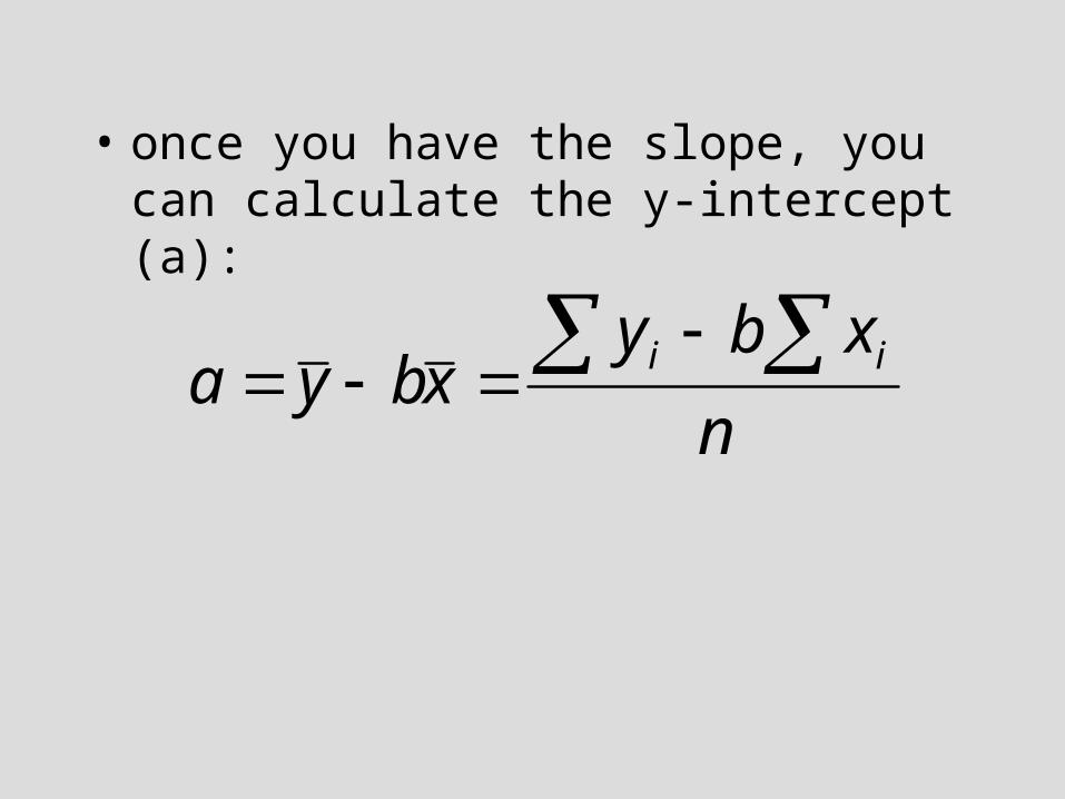
• once you have the slope, you can calculate the y-intercept (a):
n
xbyxbya ii
regression “pathologies”
• things to avoid in regression analysis
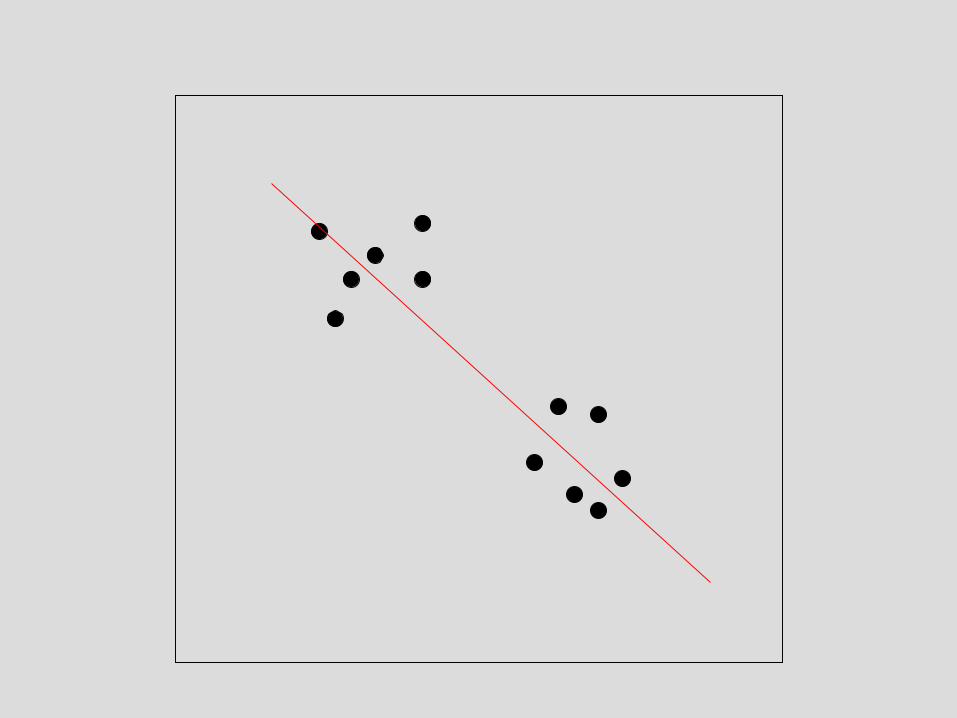
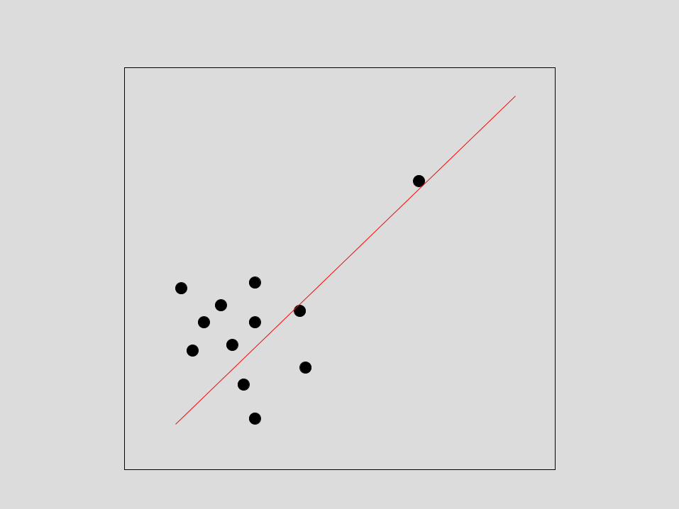
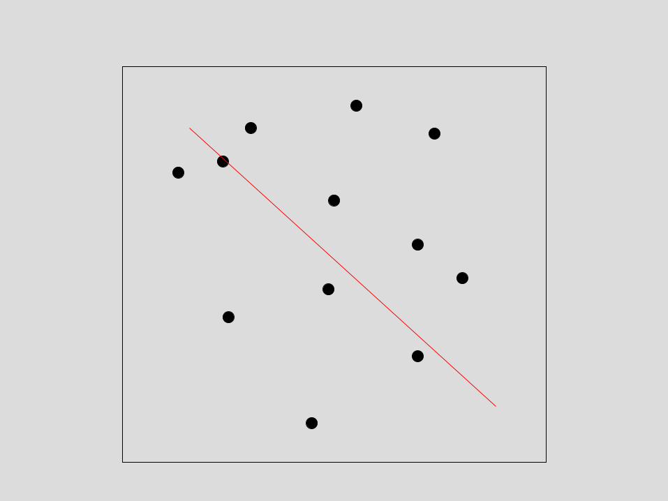
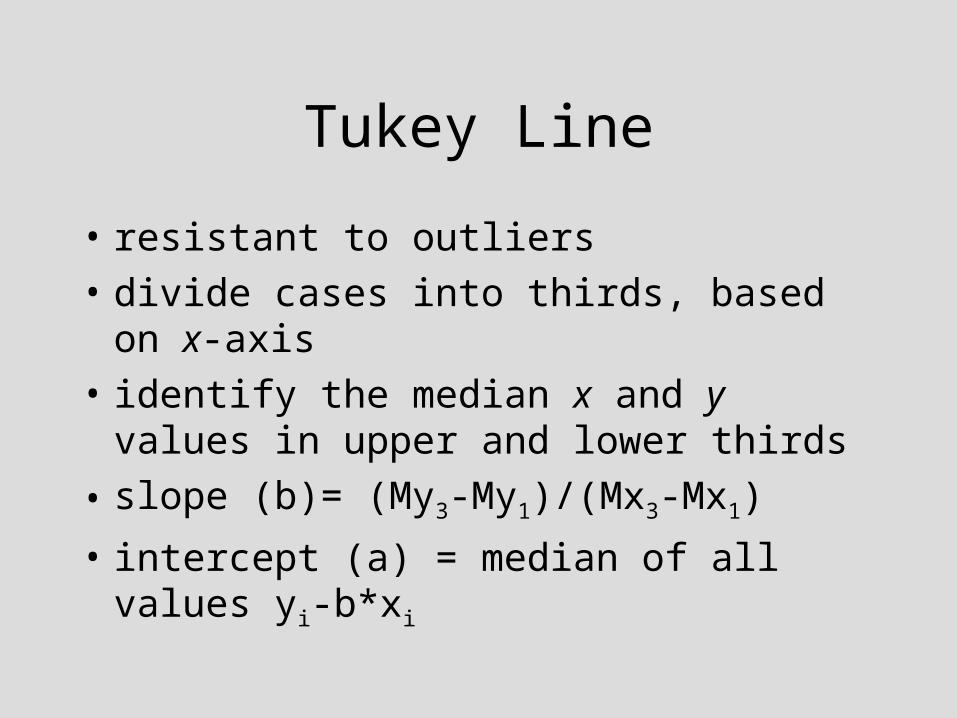
Tukey Line
• resistant to outliers
• divide cases into thirds, based on x-axis
• identify the median x and y values in upper and lower thirds
• slope (b)= (My3-My1)/(Mx3-Mx1)
• intercept (a) = median of all values yi-b*xi
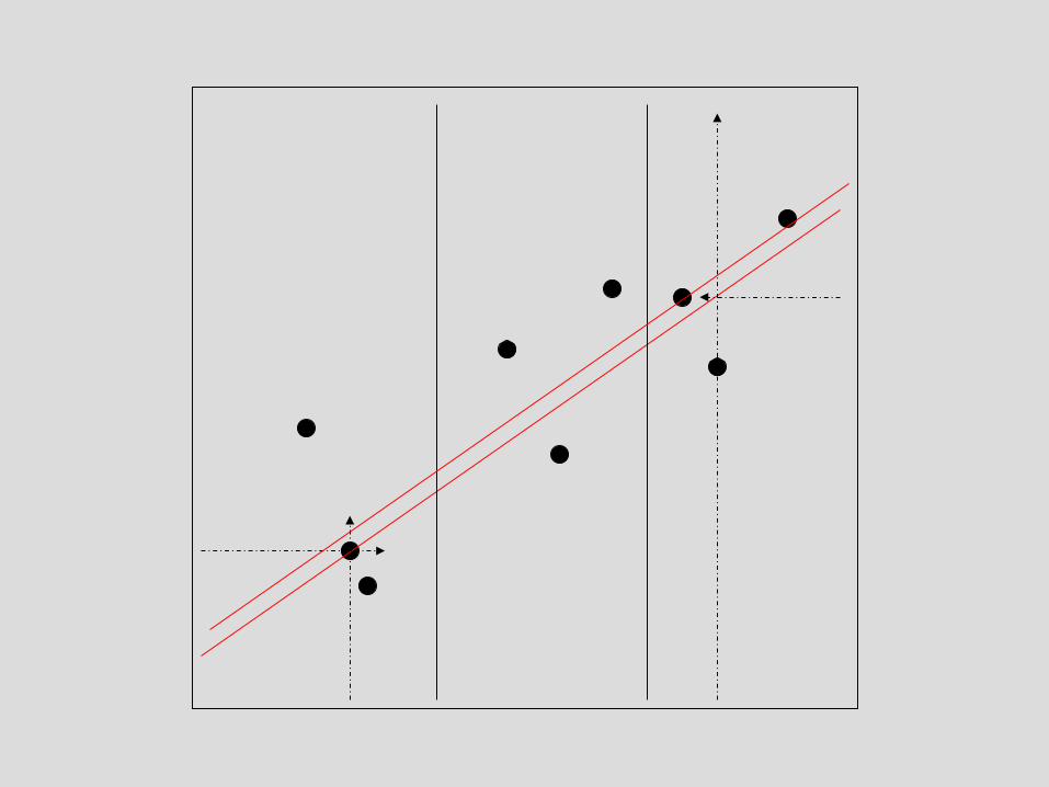
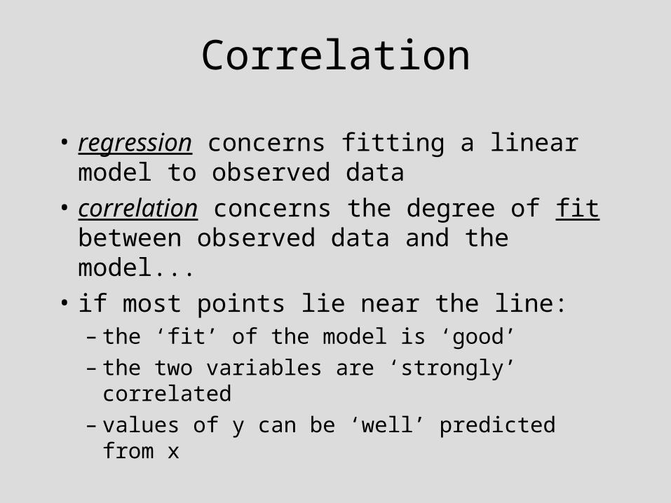
Correlation
• regression concerns fitting a linear model to observed data
• correlation concerns the degree of fit between observed data and the model...
• if most points lie near the line:– the ‘fit’ of the model is ‘good’– the two variables are ‘strongly’ correlated– values of y can be ‘well’ predicted from x
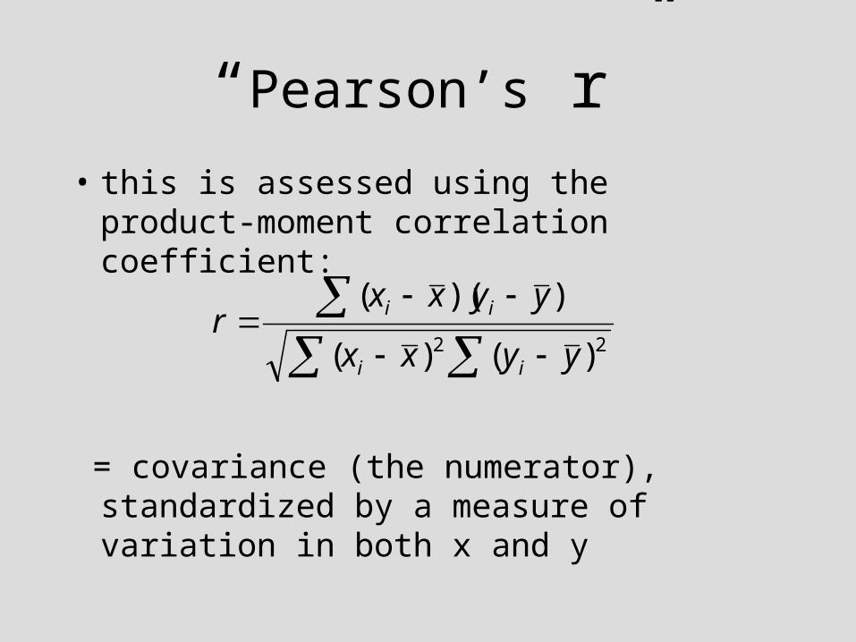
“Pearson’s r”
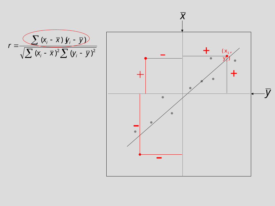
• this is assessed using the product-moment correlation coefficient:
= covariance (the numerator), standardized by a measure of variation in both x and y
22 )()(
))((
yyxx
yyxxr
ii
ii
y
x
22 )()(
))((
yyxx
yyxxr
ii
ii
+
+
-
-
(xi,yi)
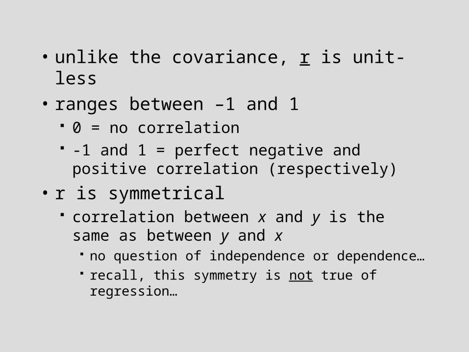
• unlike the covariance, r is unit-less
• ranges between –1 and 1 0 = no correlation -1 and 1 = perfect negative and positive
correlation (respectively)
• r is symmetrical correlation between x and y is the same as
between y and x no question of independence or dependence… recall, this symmetry is not true of regression…
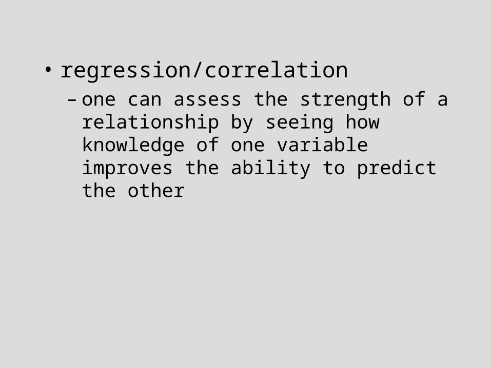
• regression/correlation– one can assess the strength of a relationship by
seeing how knowledge of one variable improves the ability to predict the other
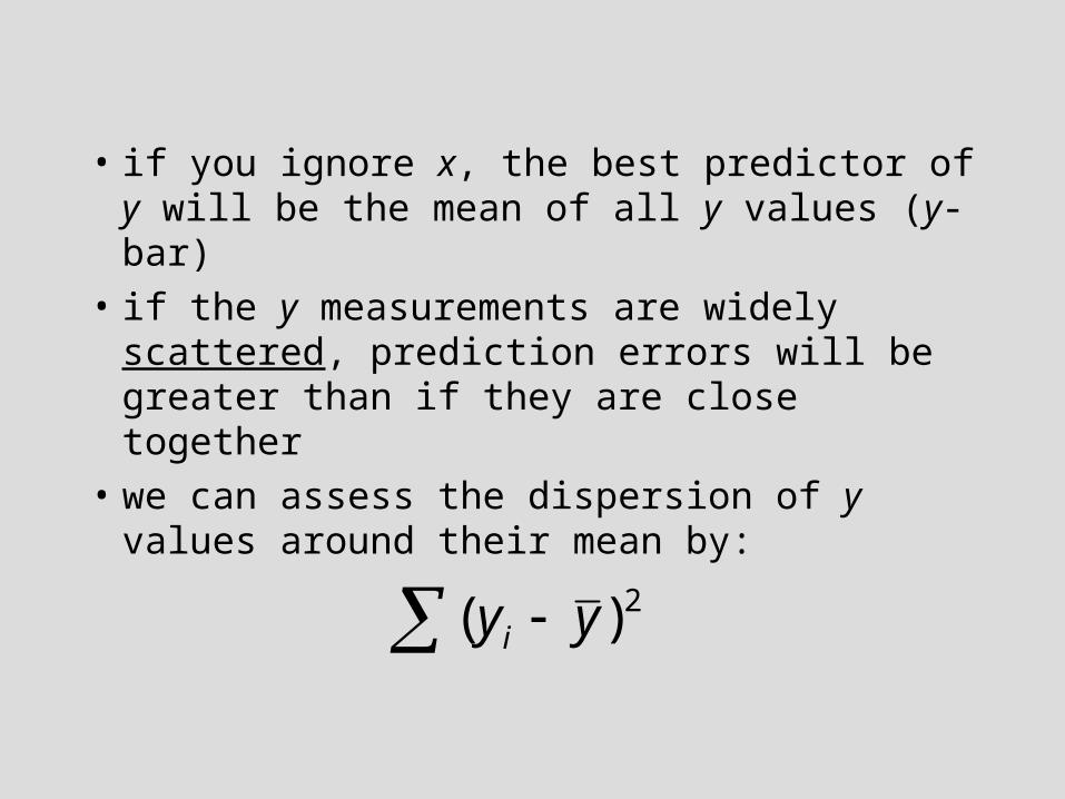
• if you ignore x, the best predictor of y will be the mean of all y values (y-bar)
• if the y measurements are widely scattered, prediction errors will be greater than if they are close together
• we can assess the dispersion of y values around their mean by:
2)( yyi

y
iy
2)( yyi
2)ˆ( ii yy
2)ˆ( ii yy
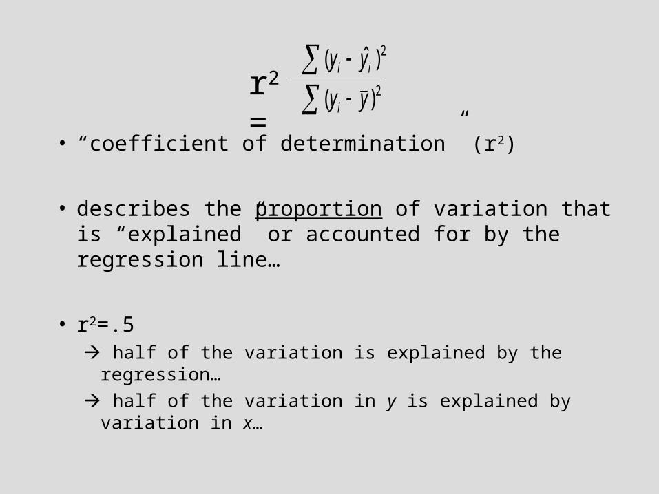
2)( yyir2=
• “coefficient of determination” (r2)
• describes the proportion of variation that is “explained” or accounted for by the regression line…
• r2=.5 half of the variation is explained by the regression…
half of the variation in y is explained by variation in x…

y
iy
correlation and percentages
• much of what we want to learn about association between variables can be learned from counts– ex: are high counts of bone needles associated
with high counts of end scrapers?
• sometimes, similar questions are posed of percent-standardized data– ex: are high proportions of decorated pottery
associated with high proportions of copper bells?
caution…
• these are different questions and have different implications for formal regression
• percents will show at least some level of correlation even if the underlying counts do not…– ‘spurious’ correlation (negative)– “closed-sum” effect
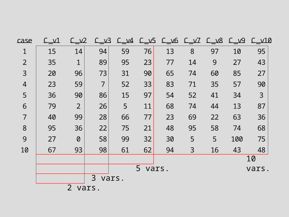
case C_v1 C_v2 C_v3 C_v4 C_v5 C_v6 C_v7 C_v8 C_v9 C_v10
1 15 14 94 59 76 13 8 97 10 95
2 35 1 89 95 23 77 14 9 27 43
3 20 96 73 31 90 65 74 60 85 27
4 23 59 7 52 33 83 71 35 57 90
5 36 90 86 15 97 54 52 41 34 3
6 79 2 26 5 11 68 74 44 13 87
7 40 99 28 66 77 23 69 22 63 36
8 95 36 22 75 21 48 95 58 74 68
9 27 0 58 99 32 30 5 5 100 75
10 67 93 98 61 62 94 3 16 43 48
10 vars.5 vars.
3 vars.2 vars.
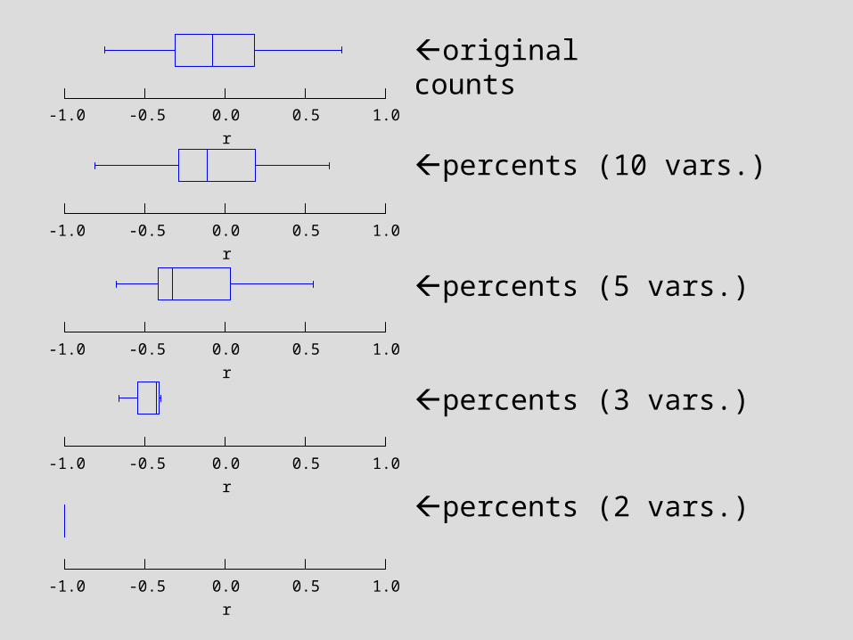
-1.0 -0.5 0.0 0.5 1.0r
original counts
-1.0 -0.5 0.0 0.5 1.0r
percents (10 vars.)
-1.0 -0.5 0.0 0.5 1.0r
percents (5 vars.)
-1.0 -0.5 0.0 0.5 1.0r
percents (3 vars.)
-1.0 -0.5 0.0 0.5 1.0r
percents (2 vars.)
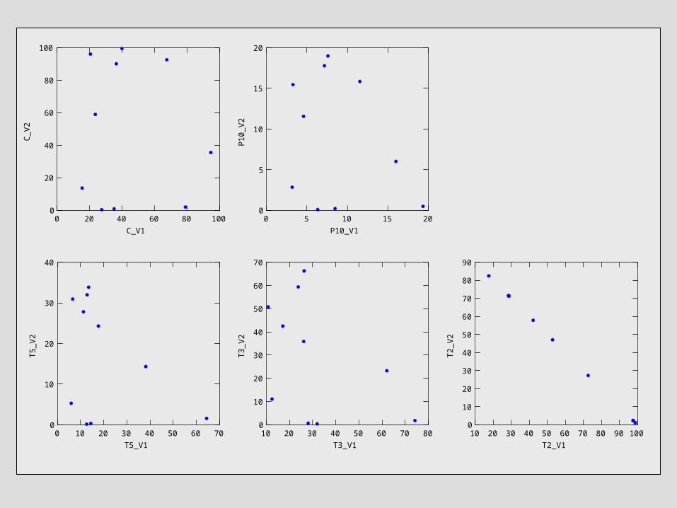
0 20 40 60 80 100C_V1
0
20
40
60
80
100
C_
V2
0 5 10 15 20P10_V1
0
5
10
15
20
P10
_V2
0 10 20 30 40 50 60 70T5_V1
0
10
20
30
40
T5_
V2
10 20 30 40 50 60 70 80T3_V1
0
10
20
30
40
50
60
70
T3_
V2
10 20 30 40 50 60 70 80 90 100T2_V1
0
10
20
30
40
50
60
70
80
90
T2_
V2
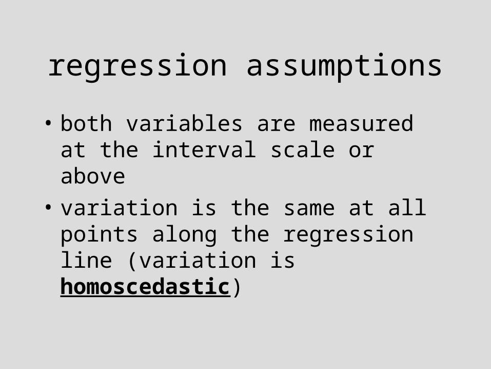
regression assumptions
• both variables are measured at the interval scale or above
• variation is the same at all points along the regression line (variation is homoscedastic)
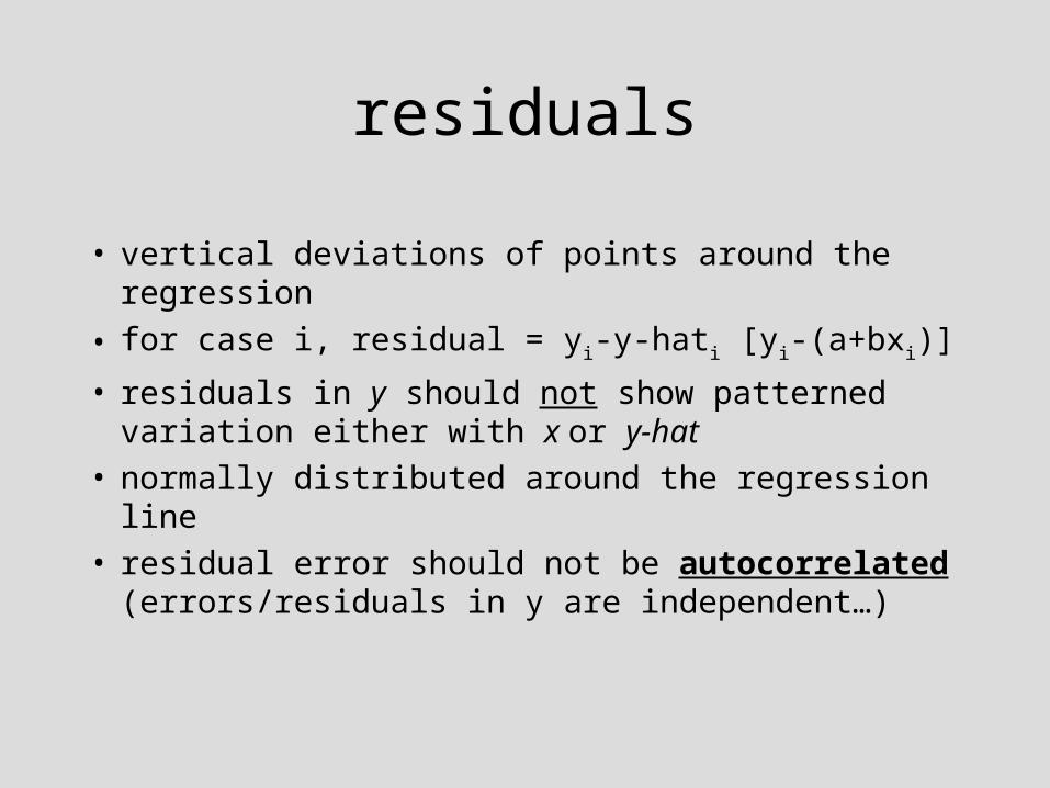
residuals
• vertical deviations of points around the regression
• for case i, residual = yi-y-hati [yi-(a+bxi)]
• residuals in y should not show patterned variation either with x or y-hat
• normally distributed around the regression line• residual error should not be autocorrelated
(errors/residuals in y are independent…)
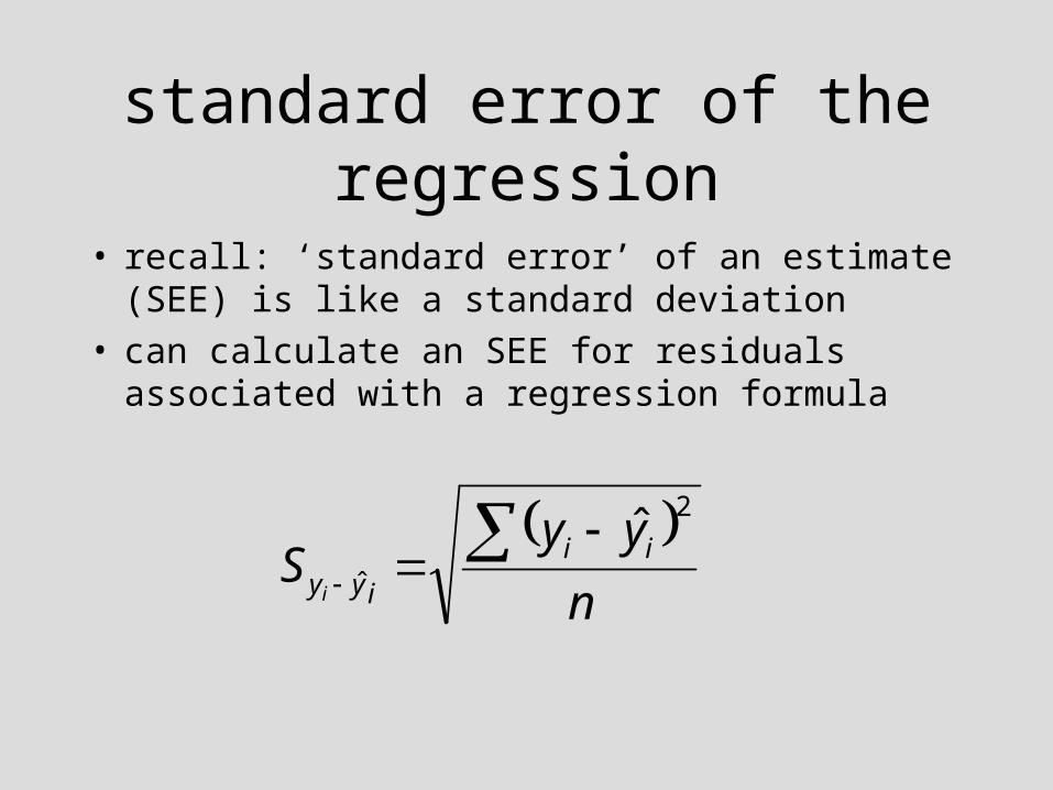
standard error of the regression
• recall: ‘standard error’ of an estimate (SEE) is like a standard deviation
• can calculate an SEE for residuals associated with a regression formula
n
yyS ii
iyyi
2
ˆ
ˆ
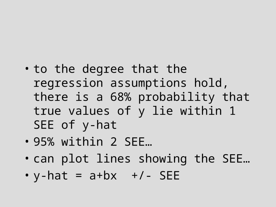
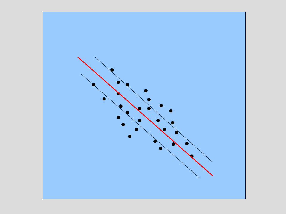
• to the degree that the regression assumptions hold, there is a 68% probability that true values of y lie within 1 SEE of y-hat
• 95% within 2 SEE…
• can plot lines showing the SEE…
• y-hat = a+bx +/- SEE
data transformations and regression
• read Shennan, Chapter 9 (esp. pp. 151-173)
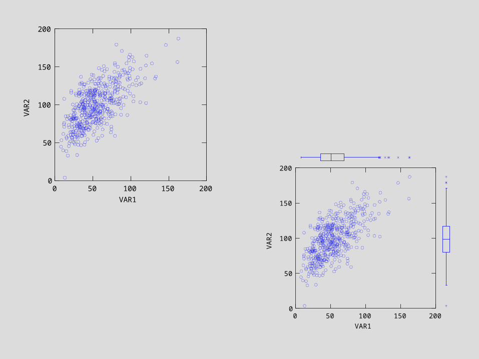
0 50 100 150 200VAR1
0
50
100
150
200
VA
R2
0 50 100 150 200VAR1
0
50
100
150
200V
AR
2
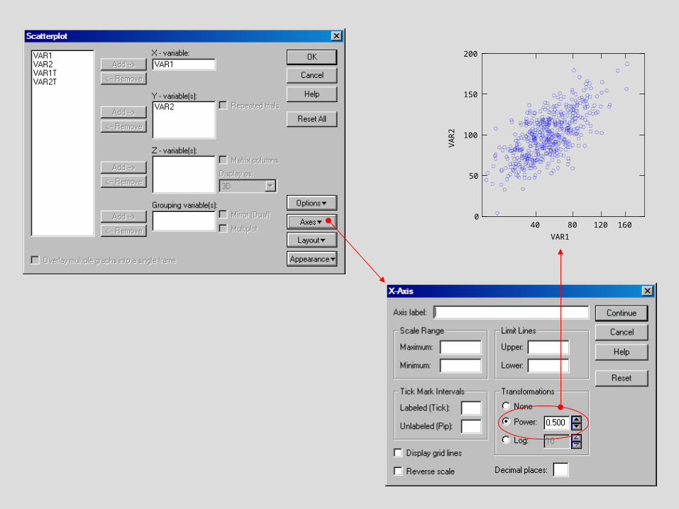
40 80 120 160VAR1
0
50
100
150
200
VA
R2
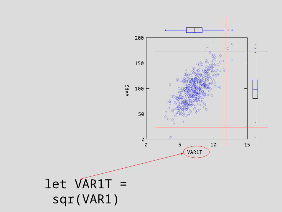
0 5 10 15VAR1T
0
50
100
150
200
VA
R2
let VAR1T = sqr(VAR1)
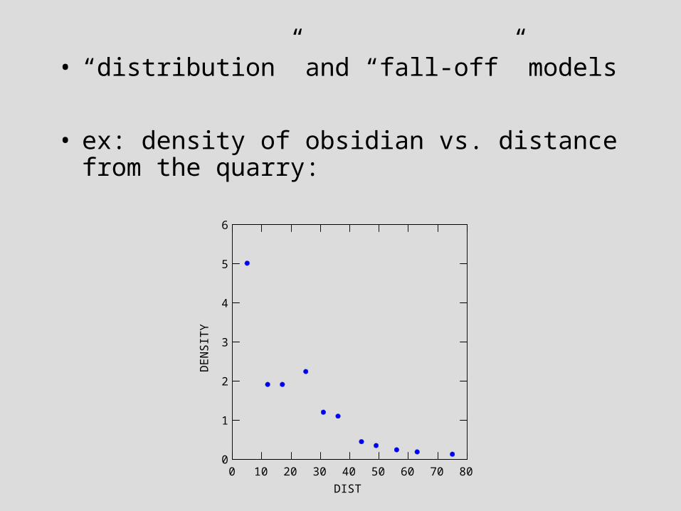
• “distribution” and “fall-off” models
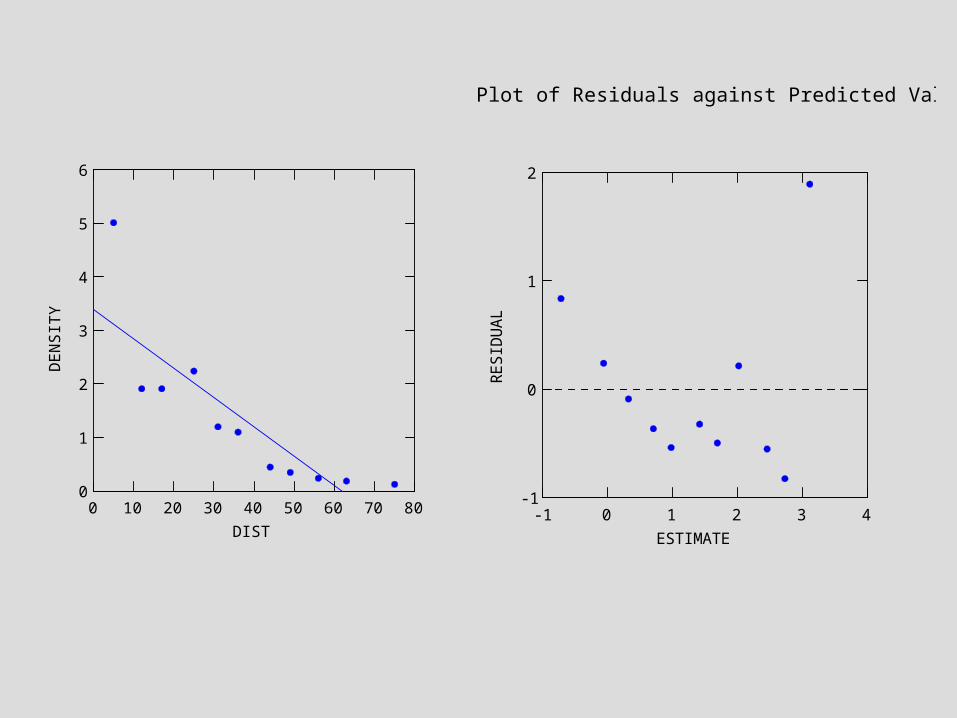
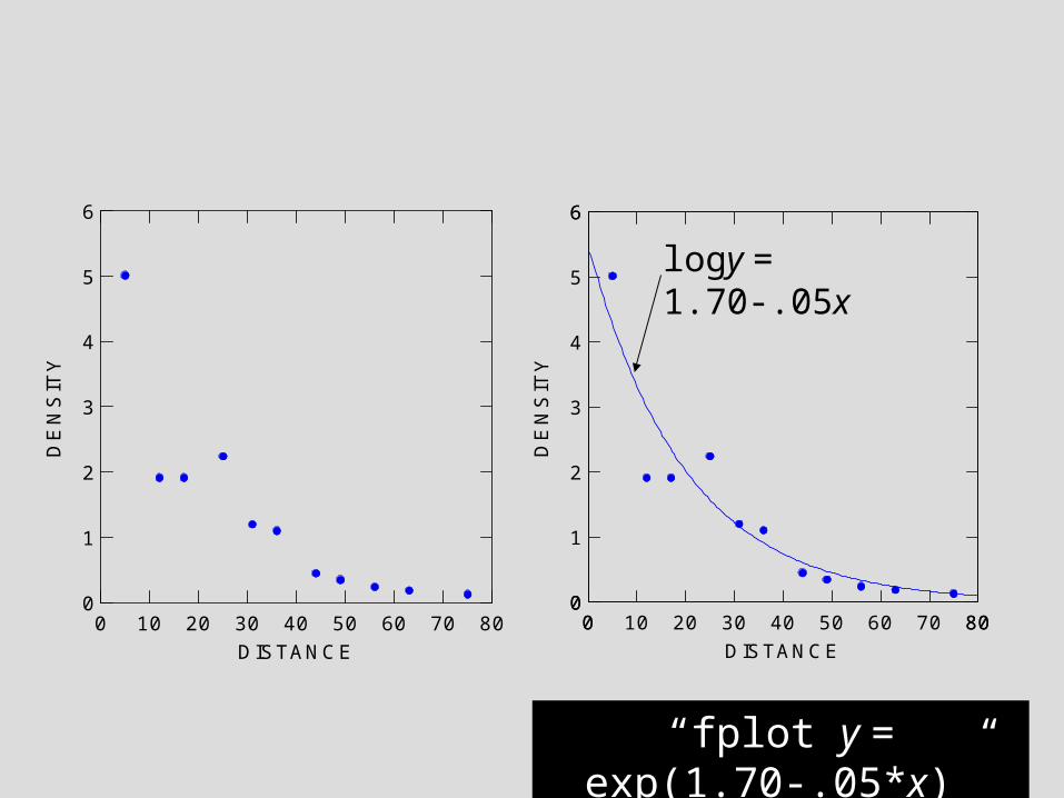
• ex: density of obsidian vs. distance from the quarry:
0 10 20 30 40 50 60 70 80DIST
0
1
2
3
4
5
6
DE
NS
ITY
0 10 20 30 40 50 60 70 80DIST
0
1
2
3
4
5
6
DE
NS
ITY
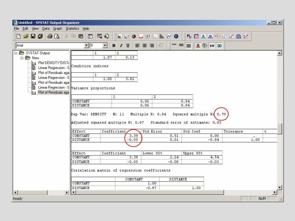
Plot of Residuals against Predicted Values
-1 0 1 2 3 4ESTIMATE
-1
0
1
2
RE
SID
UA
L
0 10 20 30 40 50 60 70 80DIST
1
2
3456
DE
NS
ITY
0 10 20 30 40 50 60 70 80DIST
-3
-2
-1
0
1
2
LG
_D
EN
S
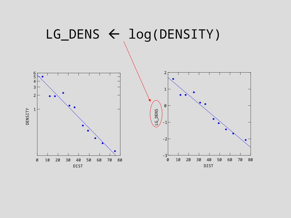
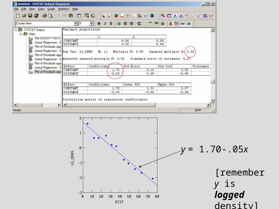
LG_DENS log(DENSITY)
0 10 20 30 40 50 60 70 80DIST
-3
-2
-1
0
1
2
LG
_D
EN
S y = 1.70-.05x
[remember y is logged density]
0 10 20 30 40 50 60 70 80DISTANCE
0
1
2
3
4
5
6
DE
NS
ITY
0 800
6
0 10 20 30 40 50 60 70 80DISTANCE
0
1
2
3
4
5
6
DE
NS
ITY
logy = 1.70-.05x
“fplot y = exp(1.70-.05*x)”
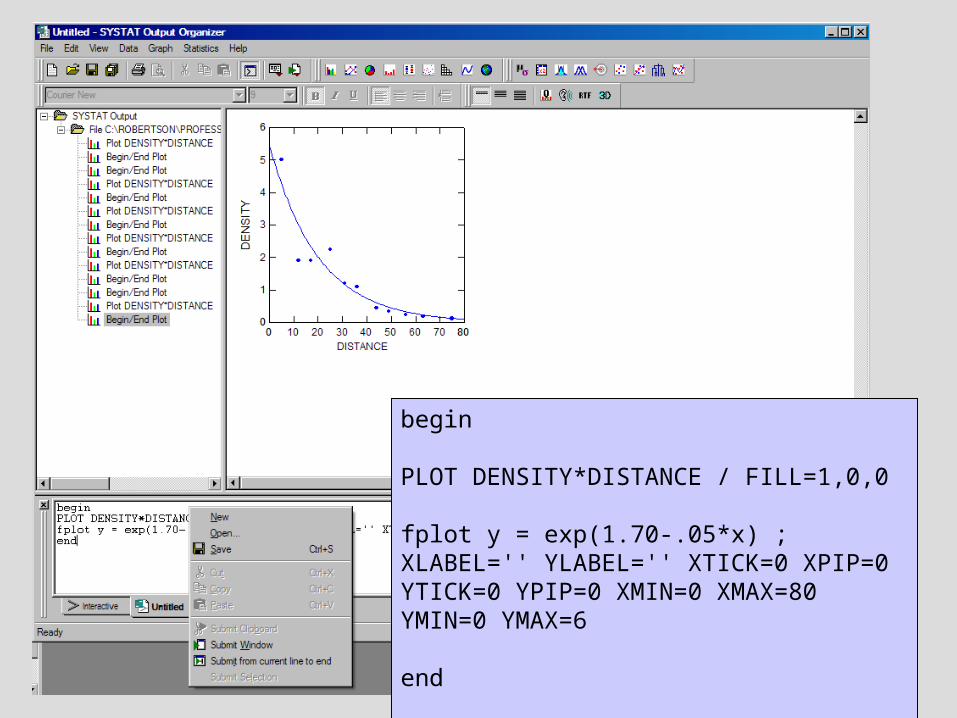
begin
PLOT DENSITY*DISTANCE / FILL=1,0,0
fplot y = exp(1.70-.05*x) ; XLABEL='' YLABEL='' XTICK=0 XPIP=0 YTICK=0 YPIP=0 XMIN=0 XMAX=80 YMIN=0 YMAX=6 end
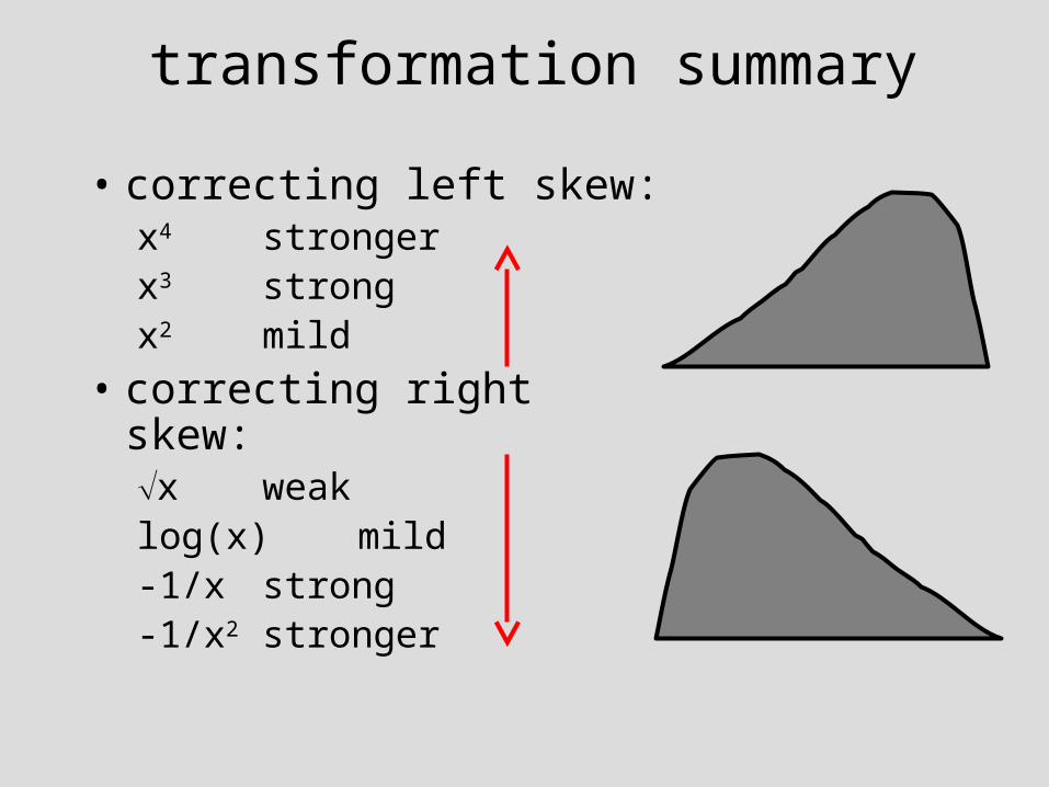
transformation summary
• correcting left skew:x4 strongerx3 strongx2 mild
• correcting right skew:x weaklog(x) mild-1/x strong-1/x2 stronger