MNRAS 000, 1–15 (2020) Preprint 17 June 2021 Compiled using MNRAS LATEX style file v3.0

Black Holes and WIMPs: All or Nothing or Something Else

Bernard Carr,1, 2? Florian Kuhnel,3† and Luca Visinelli4, 5‡1School of Physics and Astronomy, Queen Mary University of London, Mile End Road, London E1 4NS, UK2Research Center for the Early Universe, University of Tokyo, Tokyo 113-0033, Japan3Arnold Sommerfeld Center, Ludwig-Maximilians-Universitat, Theresienstraße 37, 80333 Munchen, Germany4Gravitation Astroparticle Physics Amsterdam (GRAPPA),

Institute for Theoretical Physics Amsterdam and Delta Institute for Theoretical Physics,University of Amsterdam, Science Park 904, 1098 XH Amsterdam, The Netherlands5INFN, Laboratori Nazionali di Frascati, C.P. 13, 100044 Frascati, Italy

Accepted XXX. Received YYY; in original form ZZZ

ABSTRACT

We consider constraints on primordial black holes (PBHs) in the mass range (10−18–1015)M if the dark matter

(DM) comprises weakly interacting massive particles (WIMPs) which form halos around them and generate γ-rays by

annihilations. We first study the formation of the halos and find that their density profile prior to WIMP annihilations

evolves to a characteristic power-law form. Because of the wide range of PBH masses considered, our analysis forges an

interesting link between previous approaches to this problem. We then consider the effect of the WIMP annihilations

on the halo profile and the associated generation of γ-rays. The observed extragalactic γ-ray background implies

that the PBH DM fraction is fPBH . 2× 10−9 (mχ/TeV)1.1 in the mass range 2× 10−12M (mχ/TeV)−3.2 . M .5× 1012M (mχ/TeV)1.1, where mχ and M are the WIMP and PBH masses, respectively. This limit is independent

of M and therefore applies for any PBH mass function. For M . 2 × 10−12M (mχ/TeV)−3.2, the constraint on

fPBH is a decreasing function of M and PBHs could still make a significant DM contribution at very low masses.

We also consider constraints on WIMPs if the DM is mostly PBHs. If the merging black holes recently discovered

by LIGO/Virgo are of primordial origin, this would rule out the standard WIMP DM scenario. More generally, the

WIMP DM fraction cannot exceed 10−4 for M > 10−9M and mχ > 10 GeV. There is a region of parameter space,

with M . 10−11M and mχ . 100 GeV, in which WIMPs and PBHs can both provide some but not all of the DM,

so that one requires a third DM candidate.

Key words: black hole physics – dark matter – early Universe

1 INTRODUCTION

The recent discovery of intermediate-mass black-hole mergersby the LIGO/Virgo collaboration (Abbott et al. 2020a) hasled to speculation that the dark matter (DM) might consistof black holes rather than a more conventional candidate,such as a weakly interacting massive particle (WIMP). Thisis due to the of the LIGO/Virgo black holes being producedthrough stellar collapse or multi-stage mergers. Although theLIGO/Virgo black holes might not be numerous enough toexplain all the DM, they would need to provide at least 1% ofit, which suggests the possibility of a hybrid model, in whichthe DM is some mixture of WIMPs and black holes.

If black holes provide more than 20% of the dark mat-ter, the success of the cosmological nucleosynthesis sce-nario (Wagoner et al. 1967) implies they could not derivefrom baryons and would therefore need to be primordial

? E-mail: B.J.Carr@qmul.ac.uk† E-mail: kuhnel@kth.se‡ E-mail: luca.visinelli@sjtu.edu.cn; “Fellini” Marie Curie fellow

in origin. The suggestion that the DM could be primordialblack holes (PBHs) dates back to the 1970s (Carr & Hawk-ing 1974; Chapline 1975) but has intensified over the pastthree decades, partly due to the failure to find either exper-imental or astronomical evidence for WIMPs. If PBHs havemonochromatic mass function, there are only a few mass win-dows in which they could provide all the DM but the situationis more complicated in the realistic case in which they havean extended mass function (Kuhnel et al. 2016; Carr et al.2016b; Kuhnel & Freese 2017; Carr et al. 2017). For exam-ple, one would expect the mass at which the density peaksto be less than the mass at which the LIGO/Virgo eventspeak, since the gravitational wave signal is stronger for moremassive PBHs. In particular, it has been pointed out thatthe thermal history of the Universe may naturally generatea bumpy PBH mass function, which could explain the DM,the LIGO/Virgo events and various other cosmological co-nundra (Carr et al. 2021). For a recent comprehensive reviewof these issues, see Carr & Kuhnel (2020).

Whether or not the black holes are primordial — and theanalysis of this paper will cover both cases — there is a seri-

© 2020 The Authors

arX

iv:2

011.

0193

0v4

[as

tro-

ph.C

O]

16

Jun

2021

2 B. Carr et al.

ous objection to hybrid models in which most of the DMcomprises WIMPs. This is because they would inevitablyclump in halos around the black holes, generating enhancedannihilations and γ-ray emission. As first studied by Macket al. (2007); Ricotti (2007); Ricotti et al. (2008); Ricotti &Gould (2009); Lacki & Beacom (2010) and, more recently,by Eroshenko (2016); Boucenna et al. (2018); Adamek et al.(2019); Bertone et al. (2019); Eroshenko (2020); Cai et al.(2020), this implies very stringent constraints on hybrid sce-narios, leading to the conclusion that one cannot have anappreciable amount of DM in both components.1 If nearly allthe DM is WIMPs, the fraction in black holes must be tiny;but if nearly all the DM is PBHs, the fraction in WIMPsmust be tiny.

However, this problem has only been investigated fora rather restricted combination of black hole and WIMPmasses, so the previous analysis needs to be extended to see ifthis conclusion applies more generally. For example, Adameket al. (2019) focus on the PBH mass range around 1M inwhich the WIMP velocity distribution can be neglected butallow a range of WIMP masses (10 GeV to 1 TeV); Eroshenko(2016) focuses on the subsolar PBH mass range where the ve-locity distribution must be included but assume a particularWIMP mass (70 GeV). Kadota & Silk (2021) discuss the an-nihilation of sub-GeV dark matter around PBHs. The presentanalysis uses a combination of numerical and analytical tech-niques to amalgamate these three approaches and elucidatesthe connection between them.

We must also distinguish between the Galactic and extra-galactic γ-ray backgrounds associated with WIMP annihila-tions, the constraint associated with latter being stronger forall PBH and WIMP masses. There has also been a study ofthe annihilation signal from the halo of WIMPs around thesupermassive black hole in the Galactic centre (Hooper &Goodenough 2011) and we stress that Ultracompact Miniha-los may be associated with WIMP annihilations, even if theydo not contain a central black hole (Scott & Sivertsson 2009;Josan & Green 2010; Bringmann et al. 2012). However, wedo not consider these cases here.

In a recent paper (Carr et al. 2020a), we have studiedstupendously large black holes (SLABs) in the mass range1011–1018 M. Such enormous objects might conceivably re-side in galactic nuclei, since there is already evidence for blackholes of up to 7×1010 M (Shemmer et al. 2004) in that con-text. However, our considerations were mainly motivated bythe apparent lack of constraints on PBHs in this mass range.Although SLABs are obviously too large to provide the DMin galactic halos, they might still have a large cosmologi-cal density. We found that the accretion constraints in thismass range are beset with astrophysical uncertainties, so theWIMP annihilation limit is the cleanest, at least if WIMPsprovide most of the DM. The strongest limit then comes fromthe extragalactic γ-ray background and the constraint on theDM fraction is independent of the black hole mass.

At the other extreme, it is interesting to consider the pos-sibility of stupendously small black holes, since there is stilla window in the sub-planetary (asteroid to lunar) mass range(10−16–10−10 M or 1017–1023 g) where PBHs could provide

1 The title of our paper is inspired by Lacki & Beacom (2010),who also considered constraints on the WIMP parameters.

the DM. Since these are much smaller 1M, they are nec-essarily primordial, so there is no longer the ambiguity asso-ciated with SLABs. The WIMP-annihilation constraints be-come weaker for lighter black holes, so we need to determinewhether a scenario in which both WIMPs and sub-planetaryPBHs have an appreciable density is necessarily excluded. Ifthe sum of their contributions were less than 100%, one wouldbe forced to a scenario which involves a third DM candidate.

To fill the gap in the previous literature, the purposeof this paper is to study the interplay between the DMcandidates over the PBH mass range 10−18 to 1015 Mand the WIMP mass range 10 GeV–1 TeV. Section 2 dis-cusses the thermal production of WIMPs. Section 3 deter-mines the structure of the resulting DM halos. Section 4derives the the Galactic and extragalactic γ-ray flux fromWIMP annihilations in these halos. Section 5 discusses theimplications of the recent LIGO/Virgo gravitational-waveevents are due to merging PBHs. Section 6 concludes witha discussion of future prospects. Throughout this paperwe choose units with c = kB = 1. The code used toproduce the results for this work is publicly available atgithub.com/lucavisinelli/WIMPdistributionPBH.

2 THERMAL PRODUCTION OF WIMPS

In the following, we assume that WIMPs are their own an-tiparticles and that Maxwell-Boltzmann statistics suffices indescribing the distribution of the particles. At temperaturesmuch higher than the WIMP mass mχ, the production ofWIMPs in the primordial plasma of the early Universe pro-ceeds through particle-antiparticle collisions, with rate

Γann = 〈σv〉th neq . (1)

Here, σ is the WIMP annihilation cross section, v is theWIMP relative velocity, angle brackets denote an averageover the WIMP thermal distribution (th), and n is the WIMPnumber density, with the value neq for chemical equilibrium.In more detail, the yield Y ≡ n/s in terms of the entropydensity s, evolves as (Lee & Weinberg 1977; Steigman 1979)

dY

dx=

1

3H

ds

dx〈σv〉th

(Y 2 − Y 2

eq

), (2)

where Yeq ≡ neq/s and the independent variable x ≡ mχ/Tis inversely proportional to the plasma temperature T . Thisequation assumes the conservation of entropy in a comovingvolume throughout its range of applicability. It can be solvednumerically with the initial condition Y = Yeq at x ≈ 1 toobtain the present yield Y0 and the WIMP relic density,

Ωχ h2 =

mχ s0 Y0 h2

ρcrit, (3)

where s0 is the entropy density at present time, h ≡H0/

(100 km s−1 Mpc−1

)and ρcrit = 3H2

0/(8πG) is thepresent value of the critical density.

The annihilation rate governs the Boltzmann equation thattracks the WIMP number density. At a temperature TF ≈mχ/20, the annihilation rate falls below the cosmic expansionrate, so the WIMPs cease to be produced and chemicallydecouple. For T . TF, the number of WIMPs in a comovingvolume remains approximately constant until the present.

The computation of Y0 strongly depends on the value of〈σv〉th. If we can neglect co-annihilation (Griest & Seckel

MNRAS 000, 1–15 (2020)

Black Holes and WIMPs: All or Nothing or Something Else 3

1991) and Sommerfeld enhancement (Arkani-Hamed et al.2009), we obtain (Gondolo & Gelmini 1991)

〈σv〉th =

∫ +∞4m2

χds(s− 4m2

χ

)√s K1(

√s /T )σ(s)

8m4χ T [K2(mχ/T )]2

, (4)

where s is the center-of-mass energy squared and Kν is themodified Bessel function of the second kind of order ν. If theproduct σv varies slowly with v, it can be approximated as

σv ' a+ b v2 , (5)

with constants a and b, so that 〈σv〉th = a + 3 b T/(2mχ).At lowest order in the non-relativistic expansion, 〈σannv〉th isthen independent of the WIMP velocity distribution and thesame throughout the history of the Universe.

Near resonances and thresholds where σv varies rapidlywith v, such an expansion is no longer valid, and Eq. (4) hasto be implemented more carefully. Co-annihilation can behandled in realistic models with numerical packages (Bring-mann et al. 2018; Belanger et al. 2018). In the following,we assume that chemical decoupling occurs in the radiation-dominated period of the standard model. However, onecan also consider production in non-standard cosmologicalscenarios (Gelmini & Gondolo 2006; Acharya et al. 2009;Visinelli 2018).

Following the methods outlined by Steigman et al. (2012)and Baum et al. (2017), we compute the expression for 〈σv〉ththat produces a WIMP fraction fχ = Ωχ/ΩDM through ther-mal freeze-out (Lee & Weinberg 1977; Hut 1977; Sato &Kobayashi 1977). To lowest order in T/mχ, a numerical fitgives

〈σv〉th = 〈σv〉DM f−1.0χ , (6)

where 〈σv〉DM = 2.5×10−26 cm3 s−1. This expression is validover a wide range of WIMP densities and masses above10 GeV. The only deviation from the 〈σv〉th ∝ f−1

χ behaviouris due to the changes in the relativistic degrees of freedomwith temperature.

At temperatures below TF, the relativistic plasma andWIMPs continue to exchange energy and momentum evenif the comoving number of WIMPs is fixed at the value neq.This applies as long as the Hubble rate is higher than theWIMP scattering rate (Bernstein et al. 1985), after which theWIMPs also decouple kinetically. Kinetic decoupling (KD)occurs at the temperature (Bringmann & Hofmann 2007;Visinelli & Gondolo 2015)

TKD =mχ

Γ(3/4)

(gmχ

MPl

)1/4

∼ 10 MeV( mχ

100 GeV

)5/4

, (7)

where g ≈ 10.9 for temperatures in the range 0.1–10 MeVand Γ(3/4) ≈ 1.225. The corresponding Hubble rate and timeare HKD and tKD = 1/(2HKD), respectively. Since the KDtemperature is much smaller than the WIMP mass, and sinceWIMPs are in thermal equilibrium with the plasma down toTKD due to scatterings off SM particles, we assume they havea Boltzmann velocity distribution.

3 STRUCTURE OF DARK-MATTER HALOS

PBHs form during the radiation-dominated epoch from thecollapse of mildly non-linear perturbations. It is well known

that the presence of a black hole can lead to a spike in the dis-tribution of the surrounding WIMPs. Indeed, non-relativisticWIMPs produced after freeze-out can already be gravitation-ally bound to PBHs at their formation (Ricotti et al. 2008;Lacki & Beacom 2010; Saito & Shirai 2011; Xu et al. 2020).Thereafter more WIMPs will be gravitationally attracted tothem, leading to the formation of halos whose profile dependson the WIMP velocity distribution. However, as discussed be-low, the spike distribution will be flattened sufficiently closeto the black hole by either DM scattering off plasma prior toKD or DM annihilation.

3.1 Halo formation before matter-radiation equality

A WIMP at a distance r from a PBH of mass M experiences agravitational attraction ∼ GM/r2 and a cosmic deceleration∼ H2r. The turn-around of the WIMP orbit occurs wherethese two terms are comparable at a radius ∼ (GM/H2)1/3

with H = 1/(2 t) during radiation-domination. Indeed, adetailed numerical solution for the WIMP equation of mo-tion shows that the turn-around radius is well approximatedby (Adamek et al. 2019)

rta(t) ≈ 1.0(rS t

2)1/3 , (8)

where rS = 2GM . Since a PBH has around the cosmologi-cal horizon size ∼ t at formation, the radius rta necessarilyexceeds rS thereafter and it is always smaller than the cos-mological horizon. The mass within rta remains comparableto the PBH mass until the time of matter-radiation equality,teq. Indeed, rta can be regarded as the radius of influence ofthe black hole, in the sense that it contains the same massas the black hole (Eroshenko 2016). However, the mass inWIMPs is only some fraction of this before teq.

Let us first consider the effect of PBHs which form beforetKD. From Eq. (7), these must be lighter than

MKD ∼ 103( mχ

100 GeV

)−5/2

M , (9)

which covers most of the mass range in which PBHs are usu-ally invoked. Few WIMPs are captured by the PBH prior toKD since they are tightly coupled to the primordial plasma(mainly radiation) and there is very little accretion of radia-tion before teq (Carr & Hawking 1974). However, a PBH thathas already formed at KD would be surrounded by a halo ofWIMPs up to the radius rta(tKD) with a uniform density pro-file corresponding to the background WIMP density at thatepoch, ρKD.

After tKD the halo radius will grow but the density will fallbeyond rta(tKD). Since the halo density at radius r is close tothe background WIMP density (∝ a−3) when this is the turn-around radius, the density profile is ρ(r) ∝ t−3/2 ∝ r−9/4

using Eq. (8). The WIMP halo therefore steadily grows untilteq, at which point the profile has the spike form (Adameket al. 2019)

ρχ, spike(r) = fχρeq

2

(rta(teq)

r

)9/4

[rta(tKD) < r < rta(teq)]

= fχρeq

2

(M

M

)3/4 ( rr

)9/4[r < r(M/M)1/3] ,

(10)

MNRAS 000, 1–15 (2020)

4 B. Carr et al.

where r ≡(2GM t

2eq

)1/3 ≈ 0.0193 pc is the turn-around ra-dius at teq for a solar-mass PBH and the energy density thenis ρeq = 3H2

eq m2Pl/(8π). The factor fχ ensures the WIMP

density profile scales with the WIMP fraction and the massin the WIMP halo at this stage is fχ times the PBH mass.

For PBHs which form before KD, there is also a constantdensity core within rta(tKD), so for M < MKD we can expressthe overall density profile at teq as

ρi(r) =ρχ, spike(r) ρKD

ρχ, spike(r) + ρKD. (11)

This expression reduces to ρχ, spike(r) for r rta(tKD) andρKD for r rta(tKD), with the transition occurring whereρχ, spike(r) ≈ ρKD. This is similar to taking the halo profile tobe ρi(r) = min[ρχ, spike, ρKD], as assumed by Adamek et al.(2019). We have used the form in Eq. (11) because it gives asmoother transition between the two expressions. For PBHslarger than MKD, which form after tKD, there is no constant-density core region and so Eq. (11) is inapplicable. Instead,one applies Eq. (10) over the range rS < r < rta(teq).

We refer to the expression given by Eq. (11) as the “initial”density profile. However, it is not initial in the sense that itapplies at a particular time: the density at a given value of rwithin the halo is constant and it is only the halo radius whichchanges. It is initial in the sense that it neglects two physicaleffects which modify the profile. The relationship betweenthese effects is rather obscure in previous literature, so wenow clarify this. We present the full analysis in Appendix Abut here summarise the qualitative conclusions.

The first effect is that the WIMPs are expected to havea Maxwellian velocity distribution and the low-velocity oneswill be captured by the black hole before those with the av-erage velocity σ. This problem was studied by Eroshenko(2016), who showed that Eq. (11) is replaced with a morecomplicated expression, Eq. (A1),which also depends on theWIMP velocity distribution. Starting from ρi, this yields anew distribution ρi and turns the r−9/4 profile into an r−3/2

profile at small r. However, a central core with constant den-sity ρKD is retained since the density can never exceed this.

The second effect is that the above treatment does nottake into account the orbital motion of WIMPs bound tothe PBH (i.e. it neglects their kinetic energy). This problemwas studied by Adamek et al. (2019) and concerns the meanvelocity σ rather than the low-velocity tail. (Here σ appliesat the moment of turn-around and not after virialisation.)Since the WIMP velocity decreases as a−1, the kinetic andpotential energies for WIMPs binding at a distance r fromthe PBH at the time t are

EK = kB TKD

(tKD

t

), Ep =

GMmχ

r=mχrS

2 r, (12)

where the first expression also specifies the velocity dispersionσ. Using Eq. (8) to express t in terms of r then implies thatthe ratio of the two energies is

EK

Ep=

2kB TKD

mχ

tKD√rS r

, (13)

so the kinetic term is important out to a radius

rK ≈t2KD

rS

(2kB TKD

mχ

)2

(14)

≈(mχ

MPl

)−9/2R2

Pl

rS≈ 10

( mχ

TeV

)−9/2(M

M

)−1

cm .

Outside this radius, we recover the spike solution of Eq. (10)except that the density must be multiplied by a concentrationparameter αE ≈ 1.53, as shown by Eq. (A23). We note that

rta(teq) ≈ (rS t2eq)1/3 ≈ 109 (M/M)1/3 cm , (15)

and this exceeds rK provided M < 1012 M(mχ/TeV)−27/4.Thus one expects the r−9/4 profile to develop well before thematter-dominated era.

These two effects are linked because the low-velocity tailis only important if σ is sufficiently large. For example, therecould be no such tail if σ = 0. Indeed, as shown in the Ap-pendix, both effects produce an r−3/2 tail within the radiusrK. Finally, as we show in the Appendix, a profile with ar−3/4 distribution develops at the core. The overall densityprofile is therefore

ρχ, spike(r) =

fχ ρKD

(rCr

)3/4, for r ≤ rC ,

fχρeq

2

(MM

)3/2 ( rr

)3/2for rC < r ≤ rK ,

fχρeq

2

(MM

)3/4 ( rr

)9/4for r > rK .

(16)

Here rC is the intersect of the first two lines, given by

rC ≈ rS

(mχ

TKD

)≈ 109

(M

M

)( mχ

TeV

)−1/4

cm (17)

and

r = GMteq

tKD

mχ

TKD= 1.1× 1026 cm (mχ/TeV)2.25 , (18)

and the intersect of the second two lines is the radius rK givenby Eq. (14).

At KD, Eq. (13) implies that the kinetic term can be ne-glected for (Adamek et al. 2019),

M &MK ≈ 10−5 M (mχ/TeV)−17/8 . (19)

This is also the condition rK exceeds rC, ensuring that theintermediate r−3/2 region exists. Adamek et al. were mainlyinterested in solar-mass PBHs, so only needed to confirm thatcondition (19) is well satisfied. In this paper, we consider amuch wider range of masses, including those for which theWIMP kinetic energy is important. Note that MK is muchless than MKD for mχ < 1 TeV. They also discuss the effect ofprimordial power spectrum on the halo profile but concludethat this is not important.

3.2 Halo formation after matter-radiation equality

Although Eq. (8) no longer applies after teq, because the massof the WIMP halo exceeds the mass of the black hole, thehalo continues to grow. Indeed, self-similar secondary infalland virialisation should give a DM spike with the same radialdependence as Eq. (10). This is confirmed by the numericalcalculations in Adamek et al. (2019) and can be understoodas follows. Since the black hole represents an initial overden-sity M/M for a region of mass M and density fluctuationsgrow as (1+z)−1 during the matter-dominated era, the massgravitationally bound by the PBH grows as

M(z) = M

(1 + zeq

1 + z

)(20)

after teq. Since Eq. (20) implies that the radius of the shellbinding at redshift z is r ∝ (M/ρ)1/3 ∝ (1 + z)−4/3 ∝ ρ−4/9,

MNRAS 000, 1–15 (2020)

Black Holes and WIMPs: All or Nothing or Something Else 5

this gives the same profile as Eq. (10) but it now extendsbeyond the radius rta(teq).

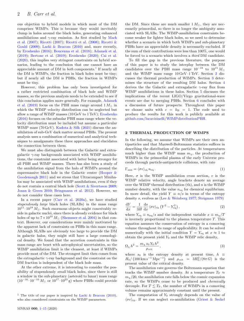
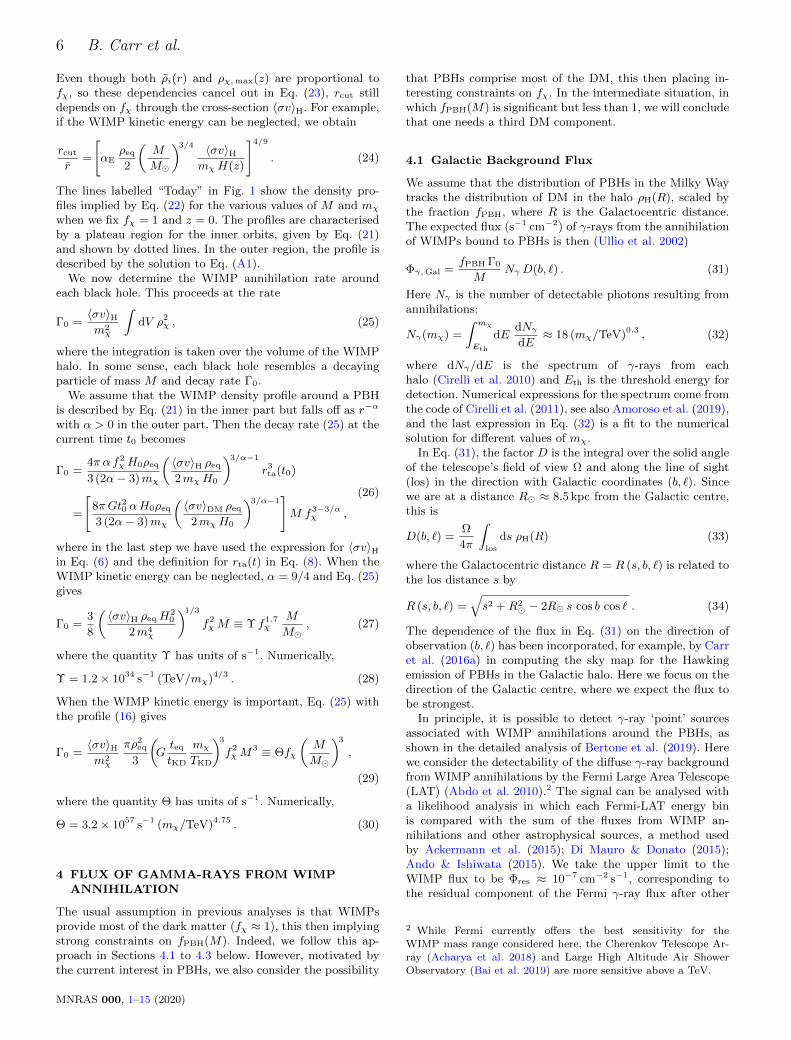
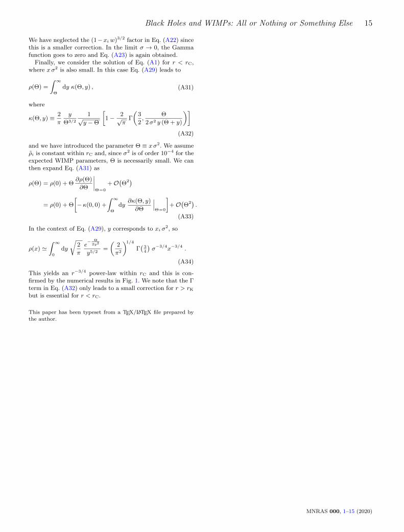
So long as one neglects the effects of WIMP annihilations,the density profiles for different values of M and mχ are asindicated by the solid lines in Fig. 1. These have been calcu-lated numerically from Eq. (A1) but their qualitative form isas anticipated above. We have set mχ = 10 GeV (magenta),mχ = 100 GeV (orange) and mχ = 1 TeV (green), this cov-ering the most plausible range of values. The upper panelshows the profiles for M = 10−12 M and M = 10−6 M,where one sees the transition from the constant-density re-gion to the r−3/2 region and then the r−9/4 region. The lowerpanel shows the profiles for M = 1M and M = 106 M. Inthis case, there is no r−3/2 region because M > MK but thereis still a constant-density region for M < MKD. The profilesare inapplicable inside the Schwarzschild radius but this isonly relevant for the lower figure.

The formation of WIMP halos around PBHs due to adia-batic accretion at late times has also been studied by Gon-dolo & Silk (1999). If the WIMPs initially have a cusp profilescaling as r−γ , the presence of the black hole leads to a spikeprofile scaling as r−γsp , where γsp = (9 − 2γ)/(4 − γ). Thisresult was first derived in Quinlan et al. (1995) and can alsobe derived from our Eq. (A1). The DM distribution aroundthe black hole is therefore steeper than in the surroundingcusp (γsp > γ) providing γ < 3, as expected in most DMmodels, and the usual result (γsp = 9/4) is obtained for aconstant density profile (γ = 0).

This analysis no longer applies after the epoch of galaxyformation, which we take to be z? ∼ 10, since the local den-sity is no longer the background cosmological density. As-trophysical processes - in particular, tidal stripping - couldmodify the WIMP halos around BHs within galaxies. Whena star passes near a BH, it deposits energy into the halo,which could remove part of it (Green & Goodwin 2007). Thismechanism has been invoked for self-gravitating halos madeof WIMPs (Schneider et al. 2010) or axions (Tinyakov et al.2016; Kavanagh et al. 2020) and it has recently been appliedto WIMP halos around BHs (Hertzberg et al. 2020). Part ofthe halo could also be removed by the interaction amongstPBH-halo systems, particularly in high-density regions suchas galactic centres or PBH clusters.

3.3 Effect of WIMP Annihilations

The WIMP population inside the halo is consumed by self-annihilation (Berezinsky et al. 1992). In order to estimatethe density of WIMPs in the core of the distribution, wecompare the inverse of the age of the halo thalo with theself-annihilation rate Γann = nχ 〈σv〉H. Here 〈σv〉H is thevelocity-weighted cross-section in the halo, where the WIMPsare assumed to have a Boltzmann velocity distribution withdispersion vrms. Setting their density to be ρχ = mχ nχ, themaximum WIMP concentration at redshift z is

ρχ,max(z) = fχmχH(z)

〈σv〉H, (21)

where we have assumed thalo teq and thalo ∼ 1/H(z), whereH(z) is the Hubble rate at redshift z. Equation (21) extendsthe result of previous literature (Ullio et al. 2002; Scott &Sivertsson 2009; Josan & Green 2010) to an arbitrary redshiftand WIMP fraction. For the Taylor expansion in Eq. (5), the

-

-

-

-

-

-

-

-

-

-

-

-

-

-

-

-

-

-

-

-

-

-

-

-

Figure 1. Density profile of WIMPs bound to a PBH of mass

M = 10−12M or M = 10−6 M (top panel) and M = 1M orM = 106 M (bottom panel) for fχ ' 1. We set mχ = 10 GeV(magenta), mχ = 100 GeV (orange) and mχ = 1 TeV (green). The

density profiles before WIMP annihilations, ρi(r), are shown by thesolid lines and derived from Eq. (A1). The density profiles after

annihilations, ρχ(r), are shown by the dotted lines and labelled“Today”. The plateau in the WIMP distribution is described byEq. (21) but does not apply for r < rS (i.e. to the left of the verticaldashed lines in the lower diagram).

velocity-averaged cross-section leads to 〈σv〉H = a+ 3 b v2rms,

so it generally differs from the thermal average 〈σv〉th whenhigher-order terms in the expansion are taken into account.In the following, we neglect these terms in the expansion ofEq. (5) and set 〈σv〉H = 〈σv〉th.

The WIMP profile is then

ρχ =ρi(r) ρχ,max(z)

ρi(r) + ρχ,max(z), (22)

with the plateau in Eq. (21) extending to the radius rcut,which from Eq. (A1) is defined implicitly by

ρi(rcut) ≈ ρχ,max(z) . (23)

MNRAS 000, 1–15 (2020)

6 B. Carr et al.

Even though both ρi(r) and ρχ,max(z) are proportional tofχ, so these dependencies cancel out in Eq. (23), rcut stilldepends on fχ through the cross-section 〈σv〉H. For example,if the WIMP kinetic energy can be neglected, we obtain

rcut

r=

[αE

ρeq

2

(M

M

)3/4 〈σv〉HmχH(z)

]4/9

. (24)

The lines labelled “Today” in Fig. 1 show the density pro-files implied by Eq. (22) for the various values of M and mχ

when we fix fχ = 1 and z = 0. The profiles are characterisedby a plateau region for the inner orbits, given by Eq. (21)and shown by dotted lines. In the outer region, the profile isdescribed by the solution to Eq. (A1).

We now determine the WIMP annihilation rate aroundeach black hole. This proceeds at the rate

Γ0 =〈σv〉Hm2χ

∫dV ρ2

χ , (25)

where the integration is taken over the volume of the WIMPhalo. In some sense, each black hole resembles a decayingparticle of mass M and decay rate Γ0.

We assume that the WIMP density profile around a PBHis described by Eq. (21) in the inner part but falls off as r−α

with α > 0 in the outer part. Then the decay rate (25) at thecurrent time t0 becomes

Γ0 =4π α f2

χH0ρeq

3 (2α− 3)mχ

(〈σv〉H ρeq

2mχH0

)3/α−1

r3ta(t0)

=

[8πGt20 αH0ρeq

3 (2α− 3)mχ

(〈σv〉DM ρeq

2mχH0

)3/α−1]M f3−3/α

χ ,

(26)

where in the last step we have used the expression for 〈σv〉Hin Eq. (6) and the definition for rta(t) in Eq. (8). When theWIMP kinetic energy can be neglected, α = 9/4 and Eq. (25)gives

Γ0 =3

8

(〈σv〉H ρeq H

20

2m4χ

)1/3

f2χM ≡ Υ f1.7

χM

M, (27)

where the quantity Υ has units of s−1. Numerically,

Υ = 1.2× 1034 s−1 (TeV/mχ)4/3 . (28)

When the WIMP kinetic energy is important, Eq. (25) withthe profile (16) gives

Γ0 =〈σv〉Hm2χ

πρ2eq

3

(Gteq

tKD

mχ

TKD

)3

f2χM

3 ≡ Θfχ

(M

M

)3

,

(29)

where the quantity Θ has units of s−1. Numerically,

Θ = 3.2× 1057 s−1 (mχ/TeV)4.75 . (30)

4 FLUX OF GAMMA-RAYS FROM WIMPANNIHILATION

The usual assumption in previous analyses is that WIMPsprovide most of the dark matter (fχ ≈ 1), this then implyingstrong constraints on fPBH(M). Indeed, we follow this ap-proach in Sections 4.1 to 4.3 below. However, motivated bythe current interest in PBHs, we also consider the possibility

that PBHs comprise most of the DM, this then placing in-teresting constraints on fχ. In the intermediate situation, inwhich fPBH(M) is significant but less than 1, we will concludethat one needs a third DM component.

4.1 Galactic Background Flux

We assume that the distribution of PBHs in the Milky Waytracks the distribution of DM in the halo ρH(R), scaled bythe fraction fPBH, where R is the Galactocentric distance.The expected flux (s−1 cm−2) of γ-rays from the annihilationof WIMPs bound to PBHs is then (Ullio et al. 2002)

Φγ,Gal =fPBH Γ0

MNγ D(b, `) . (31)

Here Nγ is the number of detectable photons resulting fromannihilations:

Nγ(mχ) =

∫ mχ

Eth

dEdNγdE

≈ 18 (mχ/TeV)0.3 , (32)

where dNγ/dE is the spectrum of γ-rays from eachhalo (Cirelli et al. 2010) and Eth is the threshold energy fordetection. Numerical expressions for the spectrum come fromthe code of Cirelli et al. (2011), see also Amoroso et al. (2019),and the last expression in Eq. (32) is a fit to the numericalsolution for different values of mχ.

In Eq. (31), the factor D is the integral over the solid angleof the telescope’s field of view Ω and along the line of sight(los) in the direction with Galactic coordinates (b, `). Sincewe are at a distance R ≈ 8.5 kpc from the Galactic centre,this is

D(b, `) =Ω

4π

∫los

ds ρH(R) (33)

where the Galactocentric distance R = R (s, b, `) is related tothe los distance s by

R (s, b, `) =√s2 +R2

− 2R s cos b cos ` . (34)

The dependence of the flux in Eq. (31) on the direction ofobservation (b, `) has been incorporated, for example, by Carret al. (2016a) in computing the sky map for the Hawkingemission of PBHs in the Galactic halo. Here we focus on thedirection of the Galactic centre, where we expect the flux tobe strongest.

In principle, it is possible to detect γ-ray ‘point’ sourcesassociated with WIMP annihilations around the PBHs, asshown in the detailed analysis of Bertone et al. (2019). Herewe consider the detectability of the diffuse γ-ray backgroundfrom WIMP annihilations by the Fermi Large Area Telescope(LAT) (Abdo et al. 2010).2 The signal can be analysed witha likelihood analysis in which each Fermi-LAT energy binis compared with the sum of the fluxes from WIMP an-nihilations and other astrophysical sources, a method usedby Ackermann et al. (2015); Di Mauro & Donato (2015);Ando & Ishiwata (2015). We take the upper limit to theWIMP flux to be Φres ≈ 10−7 cm−2 s−1, corresponding tothe residual component of the Fermi γ-ray flux after other

2 While Fermi currently offers the best sensitivity for theWIMP mass range considered here, the Cherenkov Telescope Ar-

ray (Acharya et al. 2018) and Large High Altitude Air Shower

Observatory (Bai et al. 2019) are more sensitive above a TeV.

MNRAS 000, 1–15 (2020)

Black Holes and WIMPs: All or Nothing or Something Else 7

mχ (TeV) fGalPBH fGal

χ fegPBH feg

χ

10−2 8× 10−10 3× 10−6 2× 10−11 2× 10−7

10−1 8× 10−9 2× 10−5 2× 10−10 1× 10−6

100 8× 10−8 5× 10−5 2× 10−9 5× 10−6

101 9× 10−7 2× 10−4 3× 10−8 2× 10−5

Table 1. Bounds from the Galactic (Gal) and extragalactic (eg)γ-ray flux on fPBH when the DM is mainly WIMPs and on fχwhen it is mainly PBHs for different WIMP masses. See main text

for additional discussion.

astrophysical sources are subtracted. This is about one orderof magnitude larger than the Fermi point-source sensitivity,ΦFermi = 6× 10−9 cm−2 s−1.

The condition Φγ, gal ≤ Φres yields

fPBH .ΦresM

D(b, `) Γ0Nγ(35)

≈

8.7× 10−8( mχ

TeV

)1.0(M &M∗)

3.3× 10−11( mχ

TeV

)−5.07(

10−10 MM

)2(M .M∗)

,

where M∗ is the intersect of the last two expressions,

M∗ ≈ 2× 10−12 M (mχ/TeV)−3.0 . (36)

The first expression applies when the WIMP kinetic energycan be neglected and is derived analytically from Eq. (27).The second condition includes the effect of the WIMP ki-netic energy and comes from the result given in Eq. (29).Note that M∗ is considerably less than the mass (19) wherekinetic energy can be completely neglected. This is becausethe transition is only gradual and M∗ just corresponds to theintersect of the asymptotic expressions.

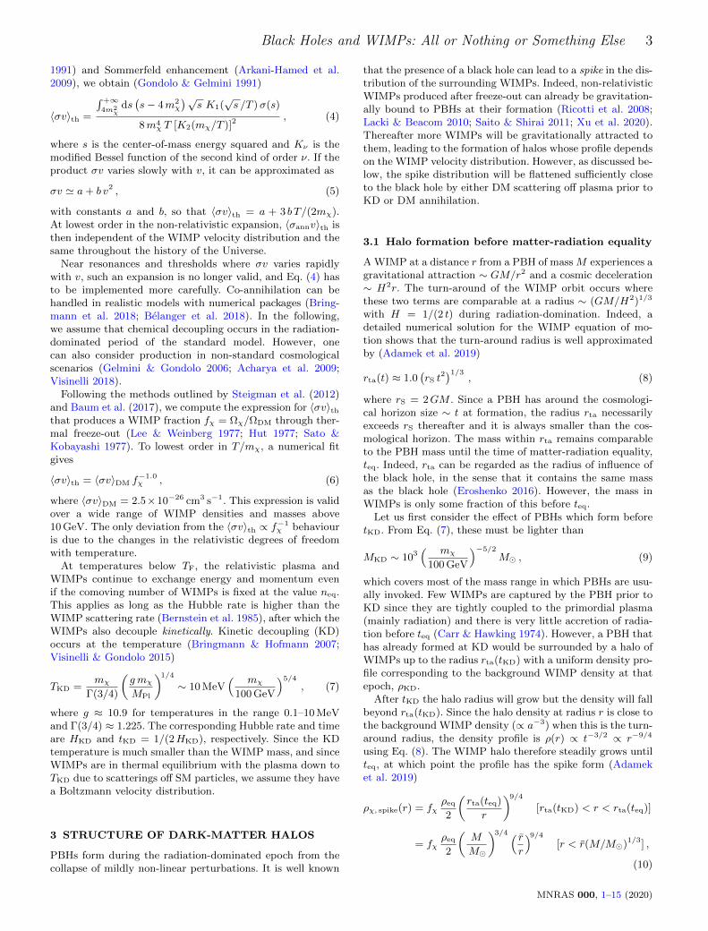
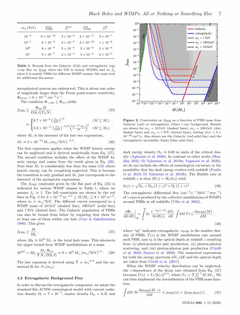
The fPBH constraint given by the flat part of Eq. (35) isindicated for various WIMP masses in Table 1, where weassume fχ ≈ 1. The full constraints are shown by the redlines in Fig. 2 for 2 × 10−12m−3.2 . M/M . 8 × 104m1.0,where m ≡ mχ/TeV. The different curves correspond to aWIMP mass of 10 GeV (dashed line), 100 GeV (solid line)and 1 TeV (dotted line). The Galactic population of PBHscan also be bound from below by requiring that there beat least one of them within our halo (Carr & Sakellariadou1999). This gives

fPBH &M

ME, (37)

where ME ≈ 1012 M is the total halo mass. This intersectsthe upper bound from WIMP annihilations at a mass

Mgal = MEMΦres

ΥNγ D(b, `)≈ 8× 104 M (mχ/TeV)1.0 . (38)

The last exponent is derived using Υ ∝ m−4/3χ and the nu-

merical fit for Nγ(mχ).

4.2 Extragalactic Background Flux

In order to discuss the extragalactic component, we adopt thestandard flat ΛCDM cosmological model with current radia-tion density Ωr = 7 × 10−5, matter density Ωm = 0.31 and

GRB

IL(extragalactic)

IL(Galactic)

--- - - -

-

-

-

-

-

-

-

-

-

-

-

-

Figure 2. Constraints on fPBH as a function of PBH mass from

Galactic (red) or extragalactic (blue) γ-ray background. Results

are shown for mχ = 10 GeV (dashed lines), mχ = 100 GeV (dot-dashed lines) and mχ = 1 TeV (dotted lines), setting 〈σv〉 = 3 ×10−26 cm3/s. Also shown are the Galactic (red solid line) and theextragalactic incredulity limits (blue solid line).

dark energy density ΩΛ ≈ 0.69 in units of the critical den-sity (Aghanim et al. 2020). In contrast to other works (Han-dley 2021; Di Valentino et al. 2019a; Vagnozzi et al. 2020),we do not include the effects of cosmological curvature or thepossibility that the dark energy evolves with redshift (Poulinet al. 2019; Di Valentino et al. 2019b). The Hubble rate atredshift z is then H(z) = H0 h(z) with

h(z) =√

ΩΛ + Ωm (1 + z)3 + Ωr (1 + z)4 . (39)

The extragalactic differential flux (cm−2 s−1 MeV−1 ster−1)of γ-rays is produced by the collective annihilations of WIMPsaround PBHs at all redshifts (Ullio et al. 2002),

dΦγdE dΩ

∣∣∣∣eg

=

∞∫0

dze−τE(z, E)

8πH(z)

dNγdE

∫dM Γ(z)

dnPBH(M)

dM,

(40)

where “eg” indicates extragalactic, nPBH is the number den-sity of PBHs, Γ(z) is the WIMP annihilation rate aroundeach PBH, and τE is the optical depth at redshift z resultingfrom (i) photon-matter pair production, (ii) photon-photonscattering, and (iii) photon-photon pair production (Cirelliet al. 2010; Slatyer et al. 2009). The numerical expressionsfor both the energy spectrum dNγ/dE and the optical depthare taken from Cirelli et al. (2011).

When the WIMP velocity distribution can be neglected,the z-dependence of the decay rate obtained from Eq. (27)becomes Γ(z) = Γ0 [h(z)]2/3, where Γ0 = Υ f1.7

χ M/M. Wecan then implement the normalisation of the PBH mass func-tion,∫

dM MdnPBH(M, z)

dM≡ ρPBH(z) = fPBH ρDM(z) , (41)

MNRAS 000, 1–15 (2020)

8 B. Carr et al.

to integrate over the mass dependence in Eq. (40). Integratingover the energy and angular dependences leads to an expres-sion for the flux

Φγ, eg =fPBH ρDM

2H0MΥ f1.7

χ Nγ(mχ) , (42)

where ρDM is the present dark matter density and Nγ is thenumber of photons produced:

Nγ(mχ) ≡∫ ∞z?

dz

∫ mχ

Eth

dEdNγdE

e−τE(z, E)

[h(z)]1/3. (43)

Here the lower limit in the redshift integral corresponds to theepoch of galaxy formation. We assume z? ∼ 10 but changingit from 10 to 15 only leads to a 5% decrease in the value ofNγ(mχ), which is much smaller than the uncertainty fromother sources.

The analysis becomes more complicated after z?. In par-ticular, if the PBHs are small enough to be inside galaxies,then the growth of the WIMP halos is no longer determinedby the background cosmological WIMP density. The halosmay also be modified or even disrupted by various dynam-ical effects. We assume z? ∼ 10 but changing it from 10 to15 only leads to a 5% decrease in the value of Nγ(mχ), in-dependent of the WIMP mass, which is much smaller thanthe uncertainty from other sources. Of course, if the PBHsare too large to be inside galaxies, then the epoch of galaxyformation is irrelevant.

Comparing the integrated flux with the Fermi sensitivityΦres yields

fPBH .2M H0 Φres

ρDM Γ0 Nγ(mχ)(44)

≈

2× 10−9 (mχ/TeV)1.1 (M &M∗)

1.1× 10−12( mχ

TeV

)−5.0(

M10−10 M

)−2

(M .M∗),

where M∗ is given by Eq. (36). The numerical bounds forthe flat part of this constraint are shown in Table 1. The fullconstraint is shown by the blue curves in Fig. 2 for a WIMPmass of 10 GeV (dashed line), 100 GeV (solid line) and 1 TeV(dotted line). We note that the extragalactic bound intersectsthe cosmological incredulity limit (37) at a mass

Meg =2H0MΦresME

αE ρDM Υ Nγ(mχ)≈ 5× 1012 M (mχ/TeV)1.1 , (45)

where we have used our fit for Nγ(mχ) and set ME ≈ρDM/H

30 ≈ 3× 1021 M.

4.3 Combined Results

We now comment on the fPBH constraints shown in Fig. 2,these applying only if WIMPs provide most of the DM.

(1) The grey region at the top left of Fig. 2, labelled “GRB”,gives the current constraint on fPBH from the soft γ-raybackground generated by PBH evaporations (Carr et al.2010, 2020b; Coogan et al. 2020). It is interesting thatWIMP annihilations also give an “effective” black hole decaylimit (Adamek et al. 2019), so both limits can be interpretedas being due to decays.

(2) The extragalactic bound is always more stringent thanthe Galactic one, the ratio being

fegPBH

fgalPBH

∼ H0 r

(Nγ(mχ)

Nγ(mχ)

)(ρH(r)

ρDM

)∼ O

(10−2) . (46)

Our argument cannot place a bound on the PBH fractionabove the mass given by Eq. (37) with ME = 1012 M(red solid line) in the Galactic case or by Eq. (46) withME = 3× 1021 M (blue solid line) in the extragalactic case.Black holes above these bounds are not expected to populatethe Galaxy or the Universe.

(3) We have included the effect of the WIMPs’ initial ve-locity distribution in computing their density profiles. Thisis important below the PBH mass indicated by Eq. (19),which corresponds to the sloping curves in Fig. 2. In thiscase, Eq. (A1) gives the halo profile, whereas the profilebefore contraction is given by Eq. (11) in the higher massrange. The WIMP profile at redshift z is then computed fromEq. (22). We note that the sloping parts of the curves in Fig. 2have been derived by Eroshenko (2016) and the flat partsby Adamek et al. (2019). However, this is the first analysisto cover the full PBH mass range.

4.4 Constraints on the WIMP population

We now extend the above analysis to the case in whichWIMPs do not provide most of the DM. The abundanceof thermally-produced WIMPs is set at the onset of theirchemical decoupling from the plasma, as discussed in Sec. 2.With the thermal freeze-out mechanism, the WIMP abun-dance is determined by properties such as the WIMP massand its interactions within the SM. Although there are cur-rently no bounds on fχ in the mass range mχ & 1 GeV, thisparameter affects the detection of γ-rays from WIMP anni-hilations (Duda et al. 2002; Baum et al. 2017).

We first modify the above analysis to place a bound onWIMPs if fPBH + fχ = 1 but with PBHs providing most ofthe DM. Since the extragalactic flux (42) is still bound by thesensitivity Φres, we can proceed as in Sec. 4.2 but consideringthe solution with fχ fPBH. The decay rate is given byEq. (26) and this leads to the extragalactic bound

fχ .

(2MH0 Φres

ρDM Γ0 Nγ(mχ)

)0.6

(47)

when the WIMP kinetic energy can be neglected. For differentvalues of the WIMP mass, this gives the bounds shown in thefifth column of Table 1. A numerical fit in this case gives fχ .5.5×10−5 (mχ/TeV)0.6 and 5×10−6 (mχ/TeV)0.7 for the forthe Galactic and extragalactic components, respectively.

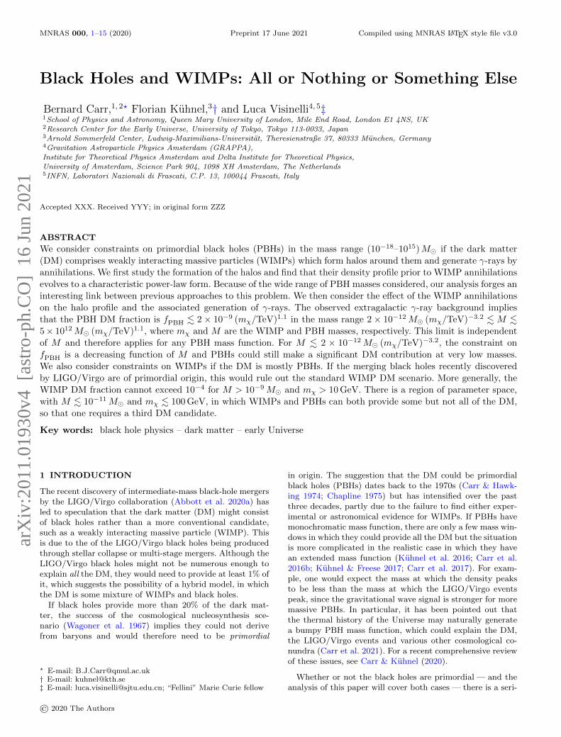
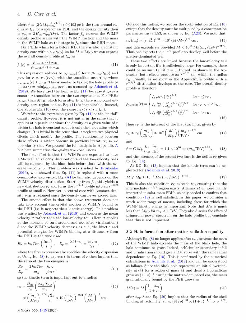
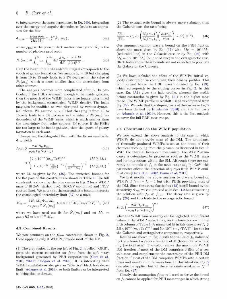
Results are shown in Fig. 3 with the values of fχ indicatedby the coloured scale as a function of M (horizontal axis) andmχ (vertical axis). The colour shows the maximum WIMPDM fraction if most of the DM comprises PBHs of a cer-tain mass and complements the constraints of the PBH DMfraction if most of the DM comprises WIMPs with a certainmass and annihilation cross-section. In this situation, Fig. 2can also be applied but all the constraints weaken as f−1.7

χ

from Eq. (27).Clearly, the assumption fPBH ≈ 1 used to derive the bound

on fχ cannot be applied for PBH mass ranges in which strong

MNRAS 000, 1–15 (2020)

Black Holes and WIMPs: All or Nothing or Something Else 9

Figure 3. The density plot shows the fraction of WIMPs fχ(colour bar) as a function of the PBH mass M (horizontal axis)

and of the WIMP mass mχ (vertical axis). We fixed fPBH+fχ = 1.

constraints on fPBH can already be placed by other argu-ments. Indeed, there are only a few mass ranges in which onecould have fPBH ≈ 1. For example, this is still possible in therange 10−15–10−10 M. In this case, depending on the valueof mχ, the WIMP abundance could vary widely and even beclose to 1. However, if PBHs in the mass range 1–10M pro-vide most of the DM, as argued by Carr et al. (2021), thenone would require fχ . 10−5 for all the WIMP masses con-sidered. One could also consider a model with an extendedPBH mass function, with a massive population attracting theWIMP halos and a lighter population providing most of theDM. This would still be compatible with the WIMP con-straint since the limit on fPBH(M) is weaker below the massM∗, given by Eq. (36), and independent of M above this.

The important point is that even a small value of fPBH

may imply a strong upper limit on fχ. For example, ifMPBH & 10−11 M and mχ . 100 GeV, both the WIMP andPBH fractions are O(10%). Since neither WIMPs nor PBHscan provide all the DM in this situation, this motivates usto consider situations in which fPBH + fχ 1, requiringthe existence of a third DM candidate (i.e. the “somethingelse” of our title). Particles which are not produced throughthe mechanisms discussed above or which avoid annihilationinclude axion-like particles (Abbott & Sikivie 1983; Dine &Fischler 1983; Preskill et al. 1983), sterile neutrinos (Dodel-son & Widrow 1994; Shi & Fuller 1999), ultra-light or “fuzzy”DM (Hu et al. 2000; Schive et al. 2014). Other forms of MA-CHOs could also serve this purpose.

5 IS SOMETHING ELSE IMPLIED BY PBHDETECTIONS?

We now briefly review several observational hints that PBHsmay exist. Each of these observations implies a lower limiton fPBH(M) for some value of M and the above argumentthen implies an upper limit on fχ well below 1. As indicatedabove, this suggests the existence of a third DM component.

LIGO/Virgo Results — The recent discovery of intermediatemass black hole mergers by the LIGO/Virgo collabora-tion (Abbott et al. 2020a) might be the first direct detectionof PBHs. It is unclear that these gravitational-wave eventsare primordial in origin, although it has been claimed thatat least some fraction must be (Franciolini et al. 2021).However, if they are, the PBH DM fraction must be largerthan 10−3. There might even be evidence for sub-solarcandidates, which could only be primordial (Phukon et al.2021).

Planetary-Mass Microlenses — Using data from the five-yearOGLE survey of 2622 microlensing events in the Galacticbulge (Mroz et al. 2017), Niikura et al. (2019) found sixultra-short ones attributable to planetary-mass objectsbetween 10−6 and 10−4 M. These would contribute O(1%)of the dark matter.

Pulsar Timing — Recently, NANOGrav has detected astochastic signal in the time residuals from their 12.5 yearpulsar-timing array data (Arzoumanian et al. 2020). Severalgroups (Kohri & Terada 2021; De Luca et al. 2021; Vaskonen& Veermae 2021; Domenech & Pi 2020; Bhattacharya et al.2020) have attributed this to a stochastic background ofgravitational waves from planetary-mass PBHs, this beingconsistent with the short timescale microlensing eventsfound in OGLE data.

Quasar Microlensing — The detection of 24 microlensedquasars by Mediavilla et al. (2017) would allow up to 25% ofgalactic halos to be PBHs in the mass range 0.05 to 0.45M.The microlensing could also be explained by interveningstars, but in several cases the stellar region of the lensinggalaxy is not aligned with the quasar, which suggests apopulation of subsolar objects with fPBH > 0.01. A relatedclaim was previously made by Hawkins (2006).

Cosmic Infrared/X-ray Backgrounds — Kashlinsky et al.(2005) and Kashlinsky (2016) have suggested that the spa-tial coherence of the X-ray and infrared source-subtractedbackgrounds could be explained by a significant density ofPBHs larger than O(1)M, the Poisson fluctuations in theirnumber density then producing halos earlier than usual. Insuch halos, a few stars form and emit infrared radiation,while the PBHs emit X-rays due to accretion.

Ultra-Faint Dwarf Galaxies — The non-detection of galaxiessmaller than 10–20 parsecs, despite their magnitude beingabove the detection limit, suggests compact halo objectsin the solar-mass range. Moreover, rapid accretion in thedensest PBH halos could explain the observed extremeUltra-Faint Dwarf Galaxies mass-to-light ratios (Clesse &Garcıa-Bellido 2018). Recent N -body simulations (Boldriniet al. 2020) support this suggestion if PBHs in the massrange 25–100M provide at least 1% of the dark matter.

If confirmed, any of these claimed signatures would ruleout the thermal WIMP model considered here from provid-ing a significant fraction of the DM. However, our analysishas disregarded the possibility that WIMP halos could bedynamically disrupted if PBHs provide most of the DM, asdiscussed by Hertzberg et al. (2020), and this might modifyour conclusion.

MNRAS 000, 1–15 (2020)

10 B. Carr et al.

6 DISCUSSIONS AND OUTLOOK

In this work, we have examined the bounds on the WIMPand PBH DM fractions from WIMP annihilations aroundPBHs with masses from 10−18 to 1015 M. Our results aresummarised in Fig. 2 for the case fPBH . fχ and in Fig. 3for the case fχ . fPBH.

We have first studied the effects of DM annihilation whenthe dominant DM component is WIMPs from thermal freeze-out. For PBHs larger than a planetary mass, the expressionfor the extragalactic γ-ray flux in Eq. (40) is independentof M , so the effect of the PBH mass function is unimpor-tant and the maximally-allowed PBH DM fraction is fPBH .2 × 10−9 (mχ/TeV)1.1 for M . 5 × 1012 M (mχ/TeV)1.1.However, the limit on fPBH is a decreasing function of massfor small M , so one could have a significant density of bothWIMPs and PBHs for M in the asteroid mass range.

We also studied the effects of DM annihilations whenthe dominant DM component is PBHs. This is particularlyrelevant for the merging intermediate-mass black holes re-cently discovered by the LIGO/Virgo collaboration (Abbottet al. 2020b,c). In particular, the collaboration has reporteda gravitational-wave signal consistent with a black hole bi-nary with component masses of 85+21

−14 M and 66+17−18 M.

It is hard to form black holes from stellar evolution in thisrange (Belczynski et al. 2016; Spera & Mapelli 2017), so thiscould indicate that the components were of primordial ori-gin. The LIGO/Virgo black holes may not provide all theDM but they must provide at least 1% of it. However, Fig. 3shows that even this would rule out the standard WIMP DMscenario, so this may require a third DM component (the‘something else’ of our title).

Alternatively, the PBHs could have an extended mass func-tion, so that fPBH = 1 even if the LIGO/Virgo black holeshave a much smaller density. In this case, the LIGO/Virgodiscovery signals a paradigm shift from microscopic to macro-scopic DM. If the PBH mass spectrum is dictated by thethermal history of the Universe, this could solve several othercosmic conundra (Carr et al. 2021).

Our limits are weakened if part of the Galactic and ex-tragalactic backgrounds is generated by some other source.For example, part of the extragalactic background can be at-tributed to TeV blazars (Abdo et al. 2009; Neronov & Vovk2010; Ghisellini et al. 2017) and part of the Galactic back-ground might come from to DM subhalos (Calore et al. 2017)or evaporating PBHs (Ackermann et al. 2018). Also super-radiant spinning BHs could interact with accreting gas togenerate another sort of BH γ-ray halo (Caputo et al. 2021).Inverse Compton scattering in the accretion disk around aBH produces photons in the keV but not γ-ray range (Sun-yaev & Truemper 1979).

Astrophysical processes could modify the WIMP halosaround BHs within galaxies. In particular, tidal strippingcould modify the halos in this case. When a star passes neara BH, it deposits energy into the halo, which could removepart of it (Green & Goodwin 2007). This mechanism has beeninvoked for self-gravitating halos made of WIMPs (Schnei-der et al. 2010) or axions (Tinyakov et al. 2016; Kavanaghet al. 2020) and it has recently been applied to WIMP ha-los around BHs (Hertzberg et al. 2020). Of course, part ofthe halo could also be removed by the interaction amongstPBH-halo systems, particularly in high-density regions such

as in the galactic centres or in PBH clusters. We leave thisfor future work.

For an individual BH, the maximum distance where γ-raysfrom DM annihilation can be detected is (Carr et al. 2020a)

dL =

√ΓNγ(mχ)

2 ΦFermi≈ 1.4 kpc

(M

M

)0.5 ( mχ

TeV

)0.82

, (48)

where we used Eqs. (27, 28) at the last step. PBHs of sub-solar mass would mostly be visible within 2 kpc of the SolarSystem, where WIMP halos should not be subject to tidalstripping. However, the assessment of this effect is very de-pendent on fPBH, M , and the orbital radius. Future MonteCarlo numerical simulations could be used to estimate theBH population in the Galaxy as a function of orbital radiusand in the Universe as a function of redshift.

Our analysis can be improved by dropping some of theassumptions made. (i) We have assumed the WIMP cross-section does not change during the evolution of the Universebut this is not true if a light mediator leads to a Sommerfeldenhancement of the WIMP annihilation (Arkani-Hamed et al.2009). (ii) The cross-section has been fixed to the value re-quired at freeze-out with standard cosmology but its valuemight vary considerably in non-standard cosmologies [e.g.with an early period of matter dominance or some other ex-otic equation of state (Gelmini & Gondolo 2008)]. (iii) Wehave assumed s-channel annihilation but the expected signalfrom annihilations must be reconsidered if the WIMP veloc-ity distribution plays a role in the computation of 〈σv〉 (e.g.if corrections of order (v/c)2 are to be taken into account).Thus our analysis does not cover other important particleDM candidates, such as the sterile neutrino (Boyarsky et al.2019) or the QCD axion (Di Luzio et al. 2020). If exotic par-ticles do form gravitationally bound structures around blackholes, they would provide a powerful cosmological test dueto their unique imprints.

Note added: Just before submission of this revised versionof our paper, a preprint by Boudaud et al. (2021) appearedwith a similar analysis of the radial profile of the WIMPdistribution to that presented below. This work was doneindependently but our Eq. (10) shows the same three power-law regimes as Boudaud et al. Although there was a mistakethe Appendix of the earlier version of our paper, this doesnot affect our constraints on the mass of the PBHs or WIMPssince the initial profile is erased by annihilations.

ACKNOWLEDGEMENTS

We thank Bradley Kavanagh and the referee for helpfulcomments. F.K. acknowledges hospitality and support fromthe Delta Institute for Theoretical Physics. L.V. acknowl-edges support from the NWO Physics Vrij Programme“The Hidden Universe of Weakly Interacting Particles”with project number 680.92.18.03 (NWO Vrije Programma),which is (partly) financed by the Dutch Research Coun-cil (NWO), as well as support from the European Union’sHorizon 2020 research and innovation programme under theMarie Sk lodowska-Curie grant agreement No. 754496 (H2020-MSCA-COFUND-2016 FELLINI).

MNRAS 000, 1–15 (2020)

Black Holes and WIMPs: All or Nothing or Something Else 11

DATA AVAILABILITY

No new data were generated or analysed in support of thisresearch.

REFERENCES

Abbott L. F., Sikivie P., 1983, Phys. Lett., B120, 133

Abbott R., et al., 2020a, Phys. Rev. Lett., 125, 101102

Abbott R., et al., 2020b, Phys. Rev. Lett., 125, 101102

Abbott R., et al., 2020c, Astrophys. J., 900, L13

Abdo A. A., et al., 2009, ApJ, 707, 1310

Abdo A. A., et al., 2010, Phys. Rev. Lett., 104, 101101

Acharya B. S., Kane G., Watson S., Kumar P., 2009, Phys. Rev.

D, 80, 083529

Acharya B., et al., 2018, Science with the Cherenkov Telescope

Array. WSP (arXiv:1709.07997), doi:10.1142/10986

Ackermann M., et al., 2015, JCAP, 09, 008

Ackermann M., et al., 2018, Astrophys. J., 857, 49

Adamek J., Byrnes C. T., Gosenca M., Hotchkiss S., 2019, Phys.

Rev., D100, 023506

Aghanim N., et al., 2020, Astron. Astrophys., 641, A6

Amoroso S., Caron S., Jueid A., Ruiz de Austri R., Skands P.,

2019, JCAP, 05, 007

Ando S., Ishiwata K., 2015, JCAP, 05, 024

Arkani-Hamed N., Finkbeiner D. P., Slatyer T. R., Weiner N.,

2009, Phys. Rev. D, 79, 015014

Arzoumanian Z., et al., 2020, Astrophys. J. Lett., 905, L34

Bai X., et al., 2019, arXiv e-prints, p. arXiv:1905.02773

Baum S., Visinelli L., Freese K., Stengel P., 2017, Phys. Rev. D,95, 043007

Belanger G., Boudjema F., Goudelis A., Pukhov A., Zaldivar B.,

2018, Comput. Phys. Commun., 231, 173

Belczynski K., et al., 2016, Astron. Astrophys., 594, A97

Berezinsky V., Gurevich A., Zybin K., 1992, Phys. Lett. B, 294,

221

Bernstein J., Brown L. S., Feinberg G., 1985, Phys. Rev. D, 32,3261

Bertone G., Coogan A. M., Gaggero D., Kavanagh B. J., Weniger

C., 2019, Phys. Rev. D, 100, 123013

Bhattacharya S., Mohanty S., Parashari P., 2020, arXiv e-prints,

p. arXiv:2010.05071

Boldrini P., Miki Y., Wagner A. Y., Mohayaee R., Silk J., ArbeyA., 2020, Mon. Not. Roy. Astron. Soc., 492, 5218

Boucenna S. M., Kuhnel F., Ohlsson T., Visinelli L., 2018, JCAP,

1807, 003

Boudaud M., Lacroix T., Stref M., Lavalle J., Salati P., 2021, arXive-prints, p. arXiv:2106.07480

Boyarsky A., Drewes M., Lasserre T., Mertens S., Ruchayskiy O.,2019, Prog. Part. Nucl. Phys., 104, 1

Bringmann T., Hofmann S., 2007, JCAP, 04, 016

Bringmann T., Scott P., Akrami Y., 2012, Phys. Rev. D, 85, 125027

Bringmann T., Edsjo J., Gondolo P., Ullio P., Bergstrom L., 2018,

JCAP, 07, 033

Cai R.-G., Yang X.-Y., Zhou Y.-F., 2020, arXiv e-prints, p.arXiv:2007.11804

Calore F., De Romeri V., Di Mauro M., Donato F., Marinacci F.,

2017, Phys. Rev. D, 96, 063009

Caputo A., Witte S. J., Blas D., Pani P., 2021, arXiv e-prints, p.

arXiv:2102.11280

Carr B. J., Hawking S., 1974, Mon. Not. Roy. Astron. Soc., 168,399

Carr B., Kuhnel F., 2020, Annual Review of Nuclear and Particle

Science, 70, 355

Carr B. J., Sakellariadou M., 1999, Astrophys. J., 516, 195

Carr B. J., Kohri K., Sendouda Y., Yokoyama J., 2010, Phys. Rev.,

D81, 104019

Carr B., Kohri K., Sendouda Y., Yokoyama J., 2016a, Phys. Rev.

D, 94, 044029

Carr B., Kuhnel F., Sandstad M., 2016b, Phys. Rev. D, 94, 083504

Carr B., Raidal M., Tenkanen T., Vaskonen V., Veermae H., 2017,Phys. Rev. D, 96, 023514

Carr B., Kuhnel F., Visinelli L., 2020a, Mon. Not. Roy. Astron.Soc.

Carr B., Kohri K., Sendouda Y., Yokoyama J., 2020b, arXiv e-prints, p. arXiv:2002.12778

Carr B., Clesse S., Garcia-Bellido J., Kuhnel F., 2021, Phys. DarkUniv., 31, 100755

Chapline G., 1975, Nature (London), 253, 251

Cirelli M., Panci P., Serpico P. D., 2010, Nucl. Phys., B840, 284

Cirelli M., et al., 2011, JCAP, 1103, 051

Clesse S., Garcıa-Bellido J., 2018, Phys. Dark Univ., 22, 137

Coogan A., Morrison L., Profumo S., 2020, arXiv e-prints, p.arXiv:2010.04797

De Luca V., Franciolini G., Riotto A., 2021, Phys. Rev. Lett., 126,041303

Di Luzio L., Giannotti M., Nardi E., Visinelli L., 2020, Phys. Rept.,870, 1

Di Mauro M., Donato F., 2015, Phys. Rev. D, 91, 123001

Di Valentino E., Melchiorri A., Silk J., 2019a, Nat. Astron., 4, 196

Di Valentino E., Ferreira R. Z., Visinelli L., Danielsson U., 2019b,Phys. Dark Univ., 26, 100385

Dine M., Fischler W., 1983, Phys. Lett., B120, 137

Dodelson S., Widrow L. M., 1994, Phys. Rev. Lett., 72, 17

Domenech G., Pi S., 2020, arXiv e-prints, p. arXiv:2010.03976

Duda G., Gelmini G., Gondolo P., 2002, Phys. Lett. B, 529, 187

Eroshenko Yu. N., 2016, Astron. Lett., 42, 347

Eroshenko Y., 2020, Int. J. Mod. Phys. A, 35, 2040046

Franciolini G., et al., 2021, arXiv e-prints, p. arXiv:2105.03349

Gelmini G. B., Gondolo P., 2006, Phys. Rev. D, 74, 023510

Gelmini G. B., Gondolo P., 2008, JCAP, 10, 002

Ghisellini G., Righi C., Costamante L., Tavecchio F., 2017, Mon.

Not. Roy. Astron. Soc., 469, 255

Gondolo P., Gelmini G., 1991, Nucl. Phys. B, 360, 145

Gondolo P., Silk J., 1999, Phys. Rev. Lett., 83, 1719

Green A. M., Goodwin S. P., 2007, Mon. Not. Roy. Astron. Soc.,

375, 1111

Griest K., Seckel D., 1991, Phys. Rev. D, 43, 3191

Handley W., 2021, Phys. Rev. D, 103, L041301

Hawkins M. R. S., 2006, Astron. Astrophys.

Hertzberg M. P., Schiappacasse E. D., Yanagida T. T., 2020, Phys.Lett. B, 807, 135566

Hooper D., Goodenough L., 2011, Phys. Lett. B, 697, 412

Hu W., Barkana R., Gruzinov A., 2000, Phys. Rev. Lett., 85, 1158

Hut P., 1977, Phys. Lett. B, 69, 85

Josan A. S., Green A. M., 2010, Phys. Rev., D82, 083527

Kadota K., Silk J., 2021, Phys. Rev. D, 103, 043530

Kashlinsky A., 2016, Astrophys.˜J., 823, L25

Kashlinsky A., Arendt R. G., Mather J., Moseley S. H., 2005,

Nature, 438, 45

Kavanagh B. J., Edwards T. D. P., Visinelli L., Weniger C., 2020,

arXiv e-prints, p. arXiv:2011.05377

Kohri K., Terada T., 2021, Phys. Lett. B, 813, 136040

Kuhnel F., Freese K., 2017, Phys. Rev. D, 95, 083508

Kuhnel F., Rampf C., Sandstad M., 2016, Eur. Phys. J. C, 76, 93

Lacki B. C., Beacom J. F., 2010, Astrophys. J., 720, L67

Lee B. W., Weinberg S., 1977, Phys. Rev. Lett., 39, 165

Mack K. J., Ostriker J. P., Ricotti M., 2007, Astrophys. J., 665,1277

Mediavilla E., Jimenez-Vicente J., Munoz J. A., Vives-Arias H.,

Calderon-Infante J., 2017, Astrophys. J., 836, L18

Mroz P., et al., 2017, Nature, 548, 183

Neronov A., Vovk I., 2010, Science, 328, 73

Niikura H., Takada M., Yokoyama S., Sumi T., Masaki S., 2019,

Phys. Rev., D99, 083503

MNRAS 000, 1–15 (2020)

12 B. Carr et al.

Peebles P. J. E., 1972, Gen.˜Relativ.˜Gravit., 3, 63

Phukon K. S., et al., 2021, arXiv e-prints, p. arXiv:2105.11449

Poulin V., Smith T., Karwal T., Kamionkowski M., 2019, Phys.

Rev. Lett., 122, 221301

Preskill J., Wise M. B., Wilczek F., 1983, Phys. Lett., B120, 127

Quinlan G. D., Hernquist L., Sigurdsson S., 1995, Astrophys.˜J.,

440, 554

Ricotti M., 2007, Astrophys. J., 662, 53

Ricotti M., Gould A., 2009, Astrophys. J., 707, 979

Ricotti M., Ostriker J. P., Mack K. J., 2008, Astrophys. J., 680,829

Saito R., Shirai S., 2011, Phys. Lett. B, 697, 95

Sato K., Kobayashi M., 1977, Prog. Theor. Phys., 58, 1775

Schive H.-Y., Chiueh T., Broadhurst T., 2014, Nature Phys., 10,

496

Schneider A., Krauss L., Moore B., 2010, Phys. Rev. D, 82, 063525

Scott P., Sivertsson S., 2009, Phys. Rev. Lett., 103, 211301

Shemmer O., Netzer H., Maiolino R., Oliva E., Croom S., Corbett

E., di Fabrizio L., 2004, Astrophys. J., 614, 547

Shi X.-D., Fuller G. M., 1999, Phys. Rev. Lett., 82, 2832

Slatyer T. R., Padmanabhan N., Finkbeiner D. P., 2009, Phys.

Rev., D80, 043526

Spera M., Mapelli M., 2017, Mon. Not. Roy. Astron. Soc., 470,

4739

Steigman G., 1979, Ann. Rev. Nucl. Part. Sci., 29, 313

Steigman G., Dasgupta B., Beacom J. F., 2012, Phys. Rev. D, 86,023506

Sunyaev R. A., Truemper J., 1979, Nature, 279, 506

Tinyakov P., Tkachev I., Zioutas K., 2016, JCAP, 01, 035

Ullio P., Zhao H., Kamionkowski M., 2001, Phys. Rev. D, 64,

043504

Ullio P., Bergstrom L., Edsjo J., Lacey C. G., 2002, Phys. Rev.,D66, 123502

Vagnozzi S., Di Valentino E., Gariazzo S., Melchiorri A., Mena O.,

Silk J., 2020, arXiv e-prints, p. arXiv:2010.02230

Vaskonen V., Veermae H., 2021, Phys. Rev. Lett., 126, 051303

Visinelli L., 2018, Symmetry, 10, 546

Visinelli L., Gondolo P., 2015, Phys. Rev. D, 91, 083526

Wagoner R. V., Fowler W. A., Hoyle F., 1967, Astrophys. J., 148,

3

Xu Z., Gong X., Zhang S.-N., 2020, Phys. Rev. D, 101, 024029

APPENDIX A: ACCRETION PRIORMATTER-RADIATION EQUALITY

In this Appendix, we analyse the form of the WIMP halo ex-pected to form around a PBH, with special emphasis on thecentral region. This problem has been analysed before but indifferent contexts, so it is interesting to clarify the relation-ship between these previous studies. Since the initial profilein the central region is ultimately hidden by the effects ofWIMP annihilations, these considerations have little impacton the constraints on the PBH and WIMP masses, so thisdiscussion is relegated to the Appendix.

There are two situations, depending on whether theWIMP’s kinetic energy is larger or smaller than the potentialenergy associated with the gravitational field of the PBH atturn-around (Adamek et al. 2019). Equation (8) for rta ne-glects the kinetic energy and only applies outside the radiusrK given by Eq. (14). This leads to an r−9/4 density profile.Within rK the kinetic energy dominates and this tends toprevent the formation of a bound halo. However, the WIMPdistribution still contains a low-velocity tail and this leadsto an r−3/2 profile in the central regions (Eroshenko 2016),

this being the key signature of the central black hole. An-other difference is that after turn-around the WIMPs tendto move inwards in the first situation and outwards in thesecond, leading to an increase and decrease in the velocitydispersion, respectively. The analysis of these two situationsis somewhat different, as we now describe.

The gravitational field of a PBH leads to a concentra-tion in the distribution of surrounding WIMPs (Ullio et al.2001). Assuming phase-space conservation, the WIMP den-sity around the PBH is (Eroshenko 2016)

ρ(r) =2

r2

∫d3vi f(vi)

∫ +∞

1

dri r2iρi(ri)

τorb

(dt

dr

), (A1)

where r is the current distance of the WIMP from the PBH,ri is its distance at turn-around, ρi(ri) is the WIMP densityprofile if one neglects kinetic energy, and vi is the WIMP ve-locity (assuming it is bound to the PBH). The velocity distri-bution function f(vi) is normalised so that ∫ d3vi f(vi) = 1.We assume this has the form

f(v) =1

(2πσ2)3/2exp

(− v2

2σ2

), (A2)

where the velocity dispersion σ is assumed to be isotropic.We normalise radii to rS = 2GM by setting

x ≡ r/rS , xi ≡ ri/rS . (A3)

Although the halo is continually growing, the density at fixedri is constant, so we can take the ‘initial’ halo profile ρi(ri)to be the profile at teq, as given by Eq. (11).

From energy conservation, the orbital period and radialspeed are

τorb = π rS z3/2 , (A4a)

dt

dr=

[1

x− 1

z−(xi vi

x

)2 (1− y2)]−1/2

, (A4b)

where

vi = |vi| , z ≡ xi/(1− xi v2i ) , y = cos θ (A5)

and θ is the angle between vi and ri, so that the angular mo-mentum is l = mχ rivi sin θ. We can then write integral (A1)as (Boucenna et al. 2018)

ρ(x) =4

x

∫dvi vif(vi)

∫dxi

xi ρi(xi)

z3/2

∫dy√

y2 + y2m

, (A6)

where

y2m ≡

(x

xi vi

)2(1

x− 1

z

)− 1 ≡ ζ2

m − 1 (A7)

with ζm ≥ 1. The range of y-integration is 1 ≥ |y| ≥ 0 andperforming this integral gives

ρ(x) =4

x

∫dvivif(vi)

∫dxi

xi ρi(xi)

z3/2ln

(ζm + 1

ζm − 1

). (A8)

As discussed later, care is required if ζm = 1 within the rangeof integration since the logarithmic term then diverges.

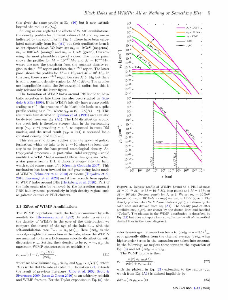
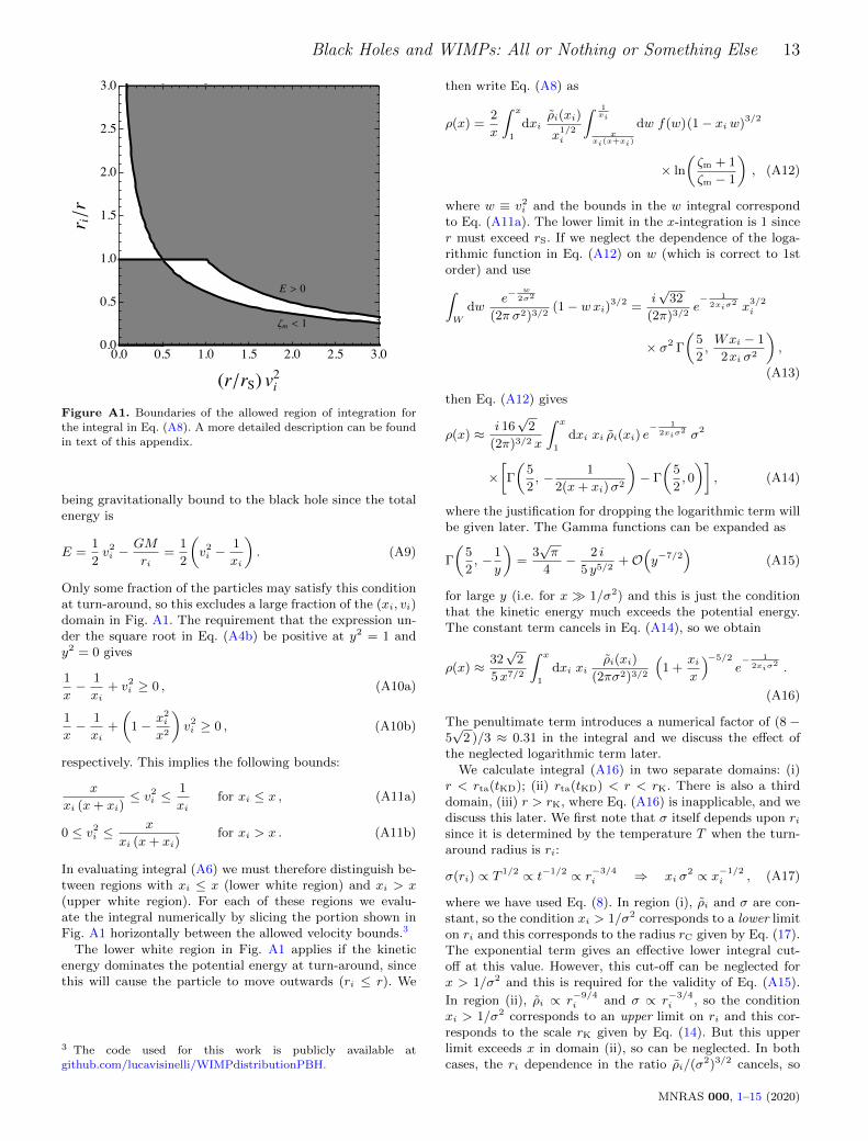
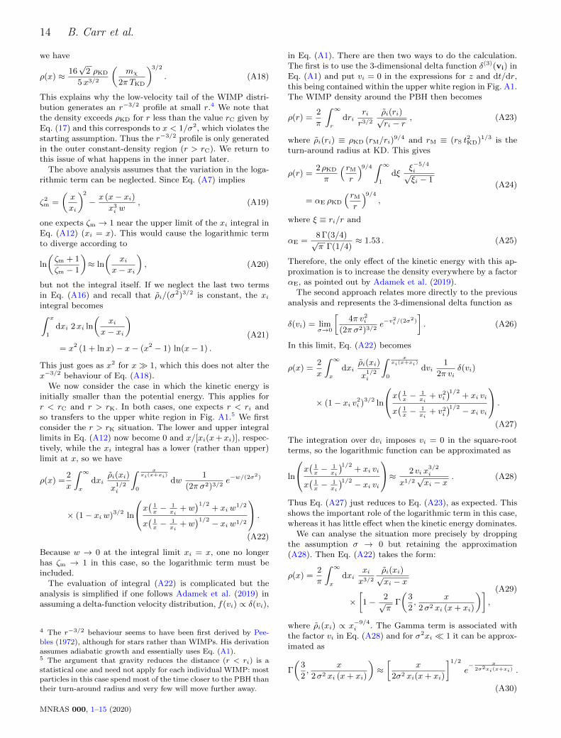
The region of (xi, vi) integration is indicated in Fig. A1. Foreach value of xi we first integrate over vi, where the velocityrange is derived as follows. Demanding that z in Eq. (A4a) bepositive yields v2

i < 1/xi and this is equivalent to the particle

MNRAS 000, 1–15 (2020)

Black Holes and WIMPs: All or Nothing or Something Else 13

Figure A1. Boundaries of the allowed region of integration forthe integral in Eq. (A8). A more detailed description can be found

in text of this appendix.

being gravitationally bound to the black hole since the totalenergy is

E =1

2v2i −

GM

ri=

1

2

(v2i −

1

xi

). (A9)

Only some fraction of the particles may satisfy this conditionat turn-around, so this excludes a large fraction of the (xi, vi)domain in Fig. A1. The requirement that the expression un-der the square root in Eq. (A4b) be positive at y2 = 1 andy2 = 0 gives

1

x− 1

xi+ v2

i ≥ 0 , (A10a)

1

x− 1

xi+

(1− x2

i

x2

)v2i ≥ 0 , (A10b)

respectively. This implies the following bounds:

x

xi (x+ xi)≤ v2

i ≤1

xifor xi ≤ x , (A11a)

0 ≤ v2i ≤

x

xi (x+ xi)for xi > x . (A11b)

In evaluating integral (A6) we must therefore distinguish be-tween regions with xi ≤ x (lower white region) and xi > x(upper white region). For each of these regions we evalu-ate the integral numerically by slicing the portion shown inFig. A1 horizontally between the allowed velocity bounds.3

The lower white region in Fig. A1 applies if the kineticenergy dominates the potential energy at turn-around, sincethis will cause the particle to move outwards (ri ≤ r). We

3 The code used for this work is publicly available at

github.com/lucavisinelli/WIMPdistributionPBH.

then write Eq. (A8) as

ρ(x) =2

x

∫ x

1

dxiρi(xi)

x1/2i

∫ 1xi

xxi(x+xi)

dw f(w)(1− xiw)3/2

× ln

(ζm + 1

ζm − 1

), (A12)

where w ≡ v2i and the bounds in the w integral correspond

to Eq. (A11a). The lower limit in the x-integration is 1 sincer must exceed rS. If we neglect the dependence of the loga-rithmic function in Eq. (A12) on w (which is correct to 1storder) and use∫W

dwe− w

2σ2

(2π σ2)3/2(1− wxi)3/2 =

i√

32

(2π)3/2e− 1

2xiσ2 x

3/2i

× σ2 Γ

(5

2,Wxi − 1

2xi σ2

),

(A13)

then Eq. (A12) gives

ρ(x) ≈ i 16√

2

(2π)3/2 x

∫ x

1

dxi xi ρi(xi) e− 1

2xiσ2 σ2

×[Γ

(5

2, − 1

2(x+ xi)σ2

)− Γ

(5

2, 0

)], (A14)

where the justification for dropping the logarithmic term willbe given later. The Gamma functions can be expanded as

Γ

(5

2, −1

y

)=

3√π

4− 2 i

5 y5/2+O

(y−7/2

)(A15)

for large y (i.e. for x 1/σ2) and this is just the conditionthat the kinetic energy much exceeds the potential energy.The constant term cancels in Eq. (A14), so we obtain

ρ(x) ≈ 32√

2

5x7/2

∫ x

1

dxi xiρi(xi)

(2πσ2)3/2

(1 +

xix

)−5/2

e− 1

2xiσ2 .

(A16)

The penultimate term introduces a numerical factor of (8 −5√

2 )/3 ≈ 0.31 in the integral and we discuss the effect ofthe neglected logarithmic term later.

We calculate integral (A16) in two separate domains: (i)r < rta(tKD); (ii) rta(tKD) < r < rK. There is also a thirddomain, (iii) r > rK, where Eq. (A16) is inapplicable, and wediscuss this later. We first note that σ itself depends upon risince it is determined by the temperature T when the turn-around radius is ri:

σ(ri) ∝ T 1/2 ∝ t−1/2 ∝ r−3/4i ⇒ xi σ

2 ∝ x−1/2i , (A17)

where we have used Eq. (8). In region (i), ρi and σ are con-stant, so the condition xi > 1/σ2 corresponds to a lower limiton ri and this corresponds to the radius rC given by Eq. (17).The exponential term gives an effective lower integral cut-off at this value. However, this cut-off can be neglected forx > 1/σ2 and this is required for the validity of Eq. (A15).

In region (ii), ρi ∝ r−9/4i and σ ∝ r

−3/4i , so the condition

xi > 1/σ2 corresponds to an upper limit on ri and this cor-responds to the scale rK given by Eq. (14). But this upperlimit exceeds x in domain (ii), so can be neglected. In bothcases, the ri dependence in the ratio ρi/(σ

2)3/2 cancels, so

MNRAS 000, 1–15 (2020)

14 B. Carr et al.

we have

ρ(x) ≈ 16√

2 ρKD

5x3/2

(mχ

2π TKD

)3/2

. (A18)

This explains why the low-velocity tail of the WIMP distri-bution generates an r−3/2 profile at small r.4 We note thatthe density exceeds ρKD for r less than the value rC given byEq. (17) and this corresponds to x < 1/σ2, which violates thestarting assumption. Thus the r−3/2 profile is only generatedin the outer constant-density region (r > rC). We return tothis issue of what happens in the inner part later.

The above analysis assumes that the variation in the loga-rithmic term can be neglected. Since Eq. (A7) implies

ζ2m =

(x

xi

)2

− x (x− xi)x3i w

, (A19)

one expects ζm → 1 near the upper limit of the xi integral inEq. (A12) (xi = x). This would cause the logarithmic termto diverge according to

ln

(ζm + 1

ζm − 1

)≈ ln

(xi

x− xi

), (A20)

but not the integral itself. If we neglect the last two termsin Eq. (A16) and recall that ρi/(σ

2)3/2 is constant, the xiintegral becomes∫ x

1

dxi 2xi ln

(xi

x− xi

)= x2 (1 + lnx)− x− (x2 − 1) ln(x− 1) .

(A21)

This just goes as x2 for x 1, which this does not alter thex−3/2 behaviour of Eq. (A18).

We now consider the case in which the kinetic energy isinitially smaller than the potential energy. This applies forr < rC and r > rK. In both cases, one expects r < ri andso transfers to the upper white region in Fig. A1.5 We firstconsider the r > rK situation. The lower and upper integrallimits in Eq. (A12) now become 0 and x/[xi(x+xi)], respec-tively, while the xi integral has a lower (rather than upper)limit at x, so we have

ρ(x) =2

x

∫ ∞x

dxiρi(xi)

x1/2i

∫ xxi(x+xi)

0

dw1

(2π σ2)3/2e−w/(2σ

2)

× (1− xiw)3/2 ln

x( 1x− 1

xi+ w

)1/2+ xiw

1/2

x(

1x− 1

xi+ w

)1/2 − xiw1/2

.

(A22)

Because w → 0 at the integral limit xi = x, one no longerhas ζm → 1 in this case, so the logarithmic term must beincluded.

The evaluation of integral (A22) is complicated but theanalysis is simplified if one follows Adamek et al. (2019) inassuming a delta-function velocity distribution, f(vi) ∝ δ(vi),

4 The r−3/2 behaviour seems to have been first derived by Pee-bles (1972), although for stars rather than WIMPs. His derivationassumes adiabatic growth and essentially uses Eq. (A1).5 The argument that gravity reduces the distance (r < ri) is a

statistical one and need not apply for each individual WIMP: mostparticles in this case spend most of the time closer to the PBH than

their turn-around radius and very few will move further away.

in Eq. (A1). There are then two ways to do the calculation.The first is to use the 3-dimensional delta function δ(3)(vi) inEq. (A1) and put vi = 0 in the expressions for z and dt/dr,this being contained within the upper white region in Fig. A1.The WIMP density around the PBH then becomes

ρ(r) =2

π

∫ ∞r

dririr3/2

ρi(ri)√ri − r

, (A23)

where ρi(ri) ≡ ρKD (rM/ri)9/4 and rM ≡ (rS t

2KD)1/3 is the

turn-around radius at KD. This gives

ρ(r) =2ρKD

π

(rM

r

)9/4 ∫ ∞1

dξξ−5/4i√ξi − 1

= αE ρKD

(rM

r

)9/4,

(A24)

where ξ ≡ ri/r and

αE =8 Γ(3/4)√π Γ(1/4)

≈ 1.53 . (A25)

Therefore, the only effect of the kinetic energy with this ap-proximation is to increase the density everywhere by a factorαE, as pointed out by Adamek et al. (2019).

The second approach relates more directly to the previousanalysis and represents the 3-dimensional delta function as

δ(vi) = limσ→0

[4π v2

i

(2π σ2)3/2e−v

2i /(2σ

2)

]. (A26)

In this limit, Eq. (A22) becomes

ρ(x) =2

x

∫ ∞x

dxiρi(xi)

x1/2i

∫ xxi(x+xi)

0

dvi1

2π viδ(vi)

× (1− xi v2i )3/2 ln

x( 1x− 1

xi+ v2

i

)1/2+ xi vi

x(

1x− 1

xi+ v2

i

)1/2 − xi vi .

(A27)

The integration over dvi imposes vi = 0 in the square-rootterms, so the logarithmic function can be approximated as

ln

x( 1x− 1

xi

)1/2+ xi vi

x(

1x− 1

xi

)1/2 − xi vi≈ 2 vi x

3/2i

x1/2√xi − x

. (A28)

Thus Eq. (A27) just reduces to Eq. (A23), as expected. Thisshows the important role of the logarithmic term in this case,whereas it has little effect when the kinetic energy dominates.

We can analyse the situation more precisely by droppingthe assumption σ → 0 but retaining the approximation(A28). Then Eq. (A22) takes the form:

ρ(x) =2

π

∫ ∞x

dxixix3/2

ρi(xi)√xi − x

×[1− 2√

πΓ

(3

2,

x

2σ2 xi (x+ xi)

)],

(A29)

where ρi(xi) ∝ x−9/4i . The Gamma term is associated with

the factor vi in Eq. (A28) and for σ2xi 1 it can be approx-imated as

Γ

(3

2,

x

2σ2 xi (x+ xi)

)≈[

x

2σ2 xi(x+ xi)

]1/2

e− x

2σ2xi(x+xi) .

(A30)

MNRAS 000, 1–15 (2020)

Black Holes and WIMPs: All or Nothing or Something Else 15

We have neglected the (1−xiw)3/2 factor in Eq. (A22) sincethis is a smaller correction. In the limit σ → 0, the Gammafunction goes to zero and Eq. (A23) is again obtained.

Finally, we consider the solution of Eq. (A1) for r < rC,where xσ2 is also small. In this case Eq. (A29) leads to

ρ(Θ) =

∫ ∞Θ

dy κ(Θ, y) , (A31)

where

κ(Θ, y) ≡ 2

π

y

Θ3/2

1√y −Θ

[1− 2√

πΓ

(3

2,

Θ

2σ2 y (Θ + y)

)](A32)

and we have introduced the parameter Θ ≡ xσ2. We assumeρi is constant within rC and, since σ2 is of order 10−4 for theexpected WIMP parameters, Θ is necessarily small. We canthen expand Eq. (A31) as

ρ(Θ) = ρ(0) + Θ∂ρ(Θ)

∂Θ

∣∣∣∣Θ=0

+O(Θ2)

= ρ(0) + Θ

[−κ(0, 0) +

∫ ∞Θ

dy∂κ(Θ, y)

∂Θ

∣∣∣Θ=0

]+O

(Θ2) .

(A33)

In the context of Eq. (A29), y corresponds to xi σ2, so

ρ(x) '∫ ∞

0

dy

√2

π

e− Θ

2y2

y5/2=

(2

π2

)1/4

Γ(

34

)σ−3/4x−3/4 .

(A34)

This yields an r−3/4 power-law within rC and this is con-firmed by the numerical results in Fig. 1. We note that the Γterm in Eq. (A32) only leads to a small correction for r > rK

but is essential for r < rC.

This paper has been typeset from a TEX/LATEX file prepared by

the author.

MNRAS 000, 1–15 (2020)