Embed Size (px)
Citation preview
Molecular Ecology (2001)
10
, 127–147
© 2001 Blackwell Science Ltd
Blackwell Science, Ltd
Tripartite genetic subdivisions in the ornate shrew (
Sorex ornatus
)
JESUS E . MALDONADO,*‡ CARLES VILÀ† and ROBERT K. WAYNE**
Department of Organismic Biology, Ecology and Evolution, University of California, Los Angeles, CA 90095–1606, USA,
†
Department of Evolutionary Biology, Uppsala University, S-752 36 Uppsala, Sweden
Abstract
We examined cytochrome
b
sequence variation in 251 ornate shrews (
Sorex ornatus
)from 20 localities distributed throughout their geographical range. Additionally, vagrant(
S. vagrans
) and montane (
S. monticolus
) shrews from four localities were used asoutgroups. We found 24 haplotypes in ornate shrews from California (USA) and BajaCalifornia (Mexico) that differed by 1–31 substitutions in 392 bp of mitochondrial DNA(mtDNA) sequence. In a subset of individuals, we sequenced 699 bp of cytochrome
b
tobetter resolve the phylogeographic relationships of populations. The ornate shrew isphylogeographically structured into three haplotype clades representing southern, centraland northern localities. Analysis of allozyme variation reveals a similar pattern of variation.Several other small California vertebrates have a similar tripartite pattern of genetic sub-division. We suggest that topographic barriers and expansion and contraction of wetlandhabitats in the central valley during Pleistocene glacial cycles account for these patterns ofgenetic variation. Remarkably, the northern ornate shrew clade is phylogenetically clus-tered with another species of shrew suggesting that it may be a unique lowland formof the vagrant shrew that evolved in parallel to their southern California counterparts.
Keywords
: allozymes, conservation, cytochrome
b
, mitochondrial DNA, phylogeography, Soricidae
Received 12 May 2000; revision received 4 September 2000; accepted 4 September 2000
Introduction
The ornate shrew (
Sorex ornatus
) is a rare species restrictedto coastal marshes and riparian communities of California,from 39
°
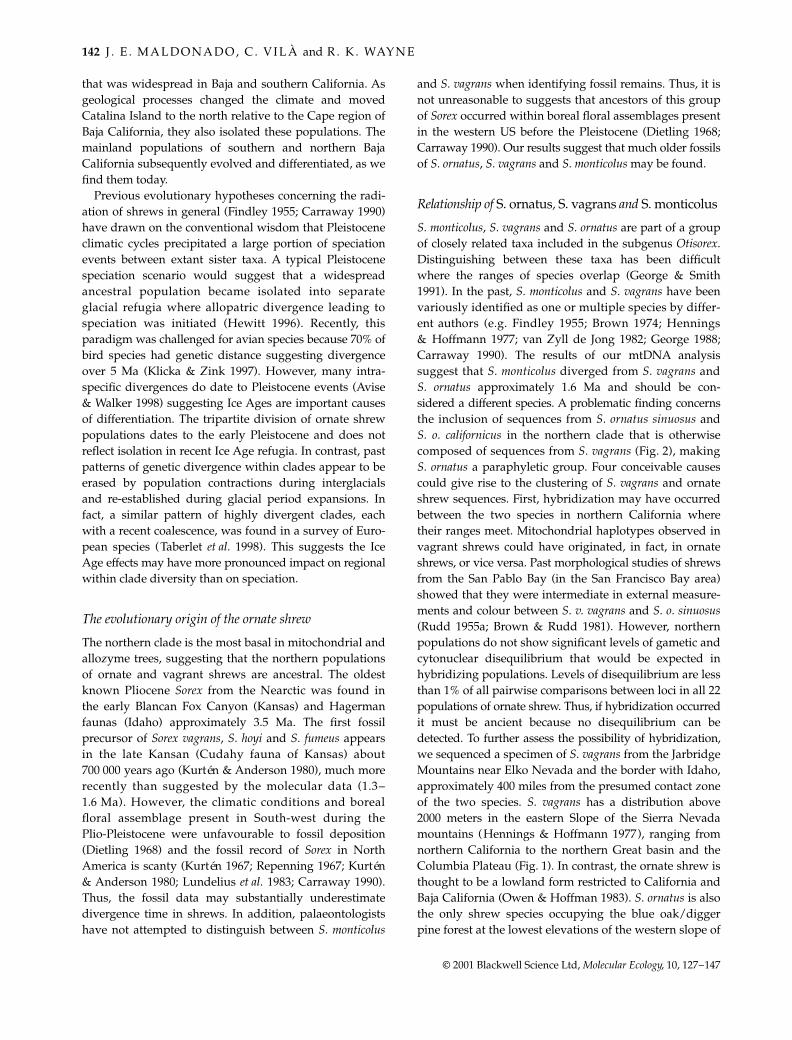
N latitude southward discontinuously to the tipof Baja California (Mexico). Nine subspecies are currentlyrecognized; two of them historically had wide distribu-tions while the other seven are found in small patchesalong coastal marshes, some inland valleys, and montanemeadows. A relictual population exists in the Sierra de laLaguna at the tip of Baja California, as well as an insularpopulation on Santa Catalina Island (Fig. 1; Owen &Hoffmann 1983).
The presence of physical and ecological barriers betweenpopulations may lead to their genetic isolation. Over time,
the phylogeny of DNA sequences from isolated popula-tions will become reciprocally monophyletic such that aphylogenetic tree of these sequences will show divisionscorresponding to the location of topographic barriers (Avise1992). Due to their small size, semifossorial habits and highdegree of habitat specialization, populations of ornate shrewsare predicted to be highly isolated. Ornate shrews arelimited to patchily distributed palustrine or salt marshhabitats (Owen & Hoffman 1983). These habitats haveincreasingly discontinuous distributions towards southernCalifornia and Baja California. In addition, the shrew’shigh basal metabolic rates require them to feed often astheir energy stores are continuously threatened by exhaus-tion (McNab 1991), further restricting long distance dis-persal. Ornate shrews rarely live more than 12–16 monthsand populations cycle annually. Summer populations arecomposed of old adults and young of the year; by autumnmost old adults have died and populations consist mainlyof young of the year that replace the parents (Rudd 1953;Newman 1976). These ecological and physiological char-acteristics put severe constraints on the ability of ornate
Correspondence: Jesus E. Maldonado. ‡Present address: Depart-ment of Conservation Biology, Molecular Genetics Laboratory,National Zoological Park, 3001 Connecticut Avenue NW,Washington, DC 20008–2598, USA. Fax: 202 6734686; E-mail:[email protected].
MEC1178.fm Page 127 Friday, December 8, 2000 3:38 PM

128
J . E . M A L D O N A D O , C . V I L À and R . K . WAY N E
© 2001 Blackwell Science Ltd,
Molecular Ecology
, 10, 127–147
shrews to occupy inhospitable habitats over long periodsof time and decrease their need for long distance dispersal.Consequently, genetic variation in the ornate shrew isexpected to be geographically partitioned.
The systematics of ornate shrews and related forms hasbeen poorly studied. Subspecies definitions in the ornateshrew often are based on the body size and pelage coloura-tion of only one or two specimens (e.g. Owen & Hoffmann1983). However, ornate shrews show a great degree ofvariation in size and pelage colouration and some popu-lations exhibit different degrees of melanism (i.e.
S. o.sinuosus, S. o. salarius
and
S. o. relictus
) so subspeciesdefinitions may not be reliable. Further, size and pelagecolouration have been shown to be an ecophenotypically
plastic character in small mammals (Patton & Brylski1987). More recently, a morphometric study of 560 ornateshrew skulls from throughout the species’ range showedlow levels of geographical differentiation and no clear-cutdifferentiation between populations or subspecies wasobserved (J. E. Maldonado
et al
. in preparation).In this paper, we measure genetic variation within and
between populations of ornate shrews using mitochon-drial DNA (mtDNA) sequences and allozyme electro-phoresis. We quantified variation in cytochrome
b,
knownto have moderate rates of evolution, over a wide range ofmammalian taxa with relatively recent divergence times(Irwin
et al
. 1991; Smith & Patton 1993; Baker
et al
. 1994;Mouchaty
et al
. 1995). We complement the mtDNA datawith a survey of nuclear encoded protein variation in 30putative loci. We find a genetic uniformity within shrewpopulations that contrasts with remarkably high levelsof divergence in mitochondrial sequence and allozymesbetween populations. Shrew populations are clusteredinto three distinct geographically defined clades that aresimilar to those found in other taxa and suggest commoncauses of genetic divergence in California vertebrates.
Materials and methods
Sample localities
Sampling sites in California and Baja California includetopographically and ecologically diverse locales, includingcoastal marshes, enclosed basins and valleys, and mountainranges (Fig. 1). The type localities of six of seven restrictedrange subspecies [
Sorex ornatus sinuosus, S. o. salarius,S. o. relictus, S. o. salicornicus
(three localities),
S. o. willetti
,
S. o. lagunae
] were sampled (Fig. 1 and Table 1). For
S. o.juncensis,
the habitat in the type locality was highly degradedand the subspecies could be extinct (Maldonado 1999).Instead, two neighbouring populations of
S. o. ornatus
were sampled (populations 18 and 19 in Fig. 1). Threepopulations from the northern widely distributed subspecies(
S. o. californicus
) and eight populations from the mostwidely distributed southern subspecies (
S. o. ornatus
)were also sampled. Finally, samples collected in northernCalifornia, around Shasta Lake (population 1 in Fig. 1),outside the range recognized for
S. ornatus
, were included.This population was identified as
S. ornatus
by its externalmorphology, and was different from
S. vagrans
living athigher altitudes in the same area. Two other shrew speciesfrom the genus
Sorex
that live in California, the montaneshrew,
S. monticolus,
and the vagrant shrew,
S. vagrans,
were also sampled. These species were previously deter-mined to be closely related to ornate shrews based onmorphological (Findley 1955; Junge & Hoffmann 1981;Carraway 1990) and allozyme studies (George 1988) andoccur at higher elevations (Williams 1991). The only
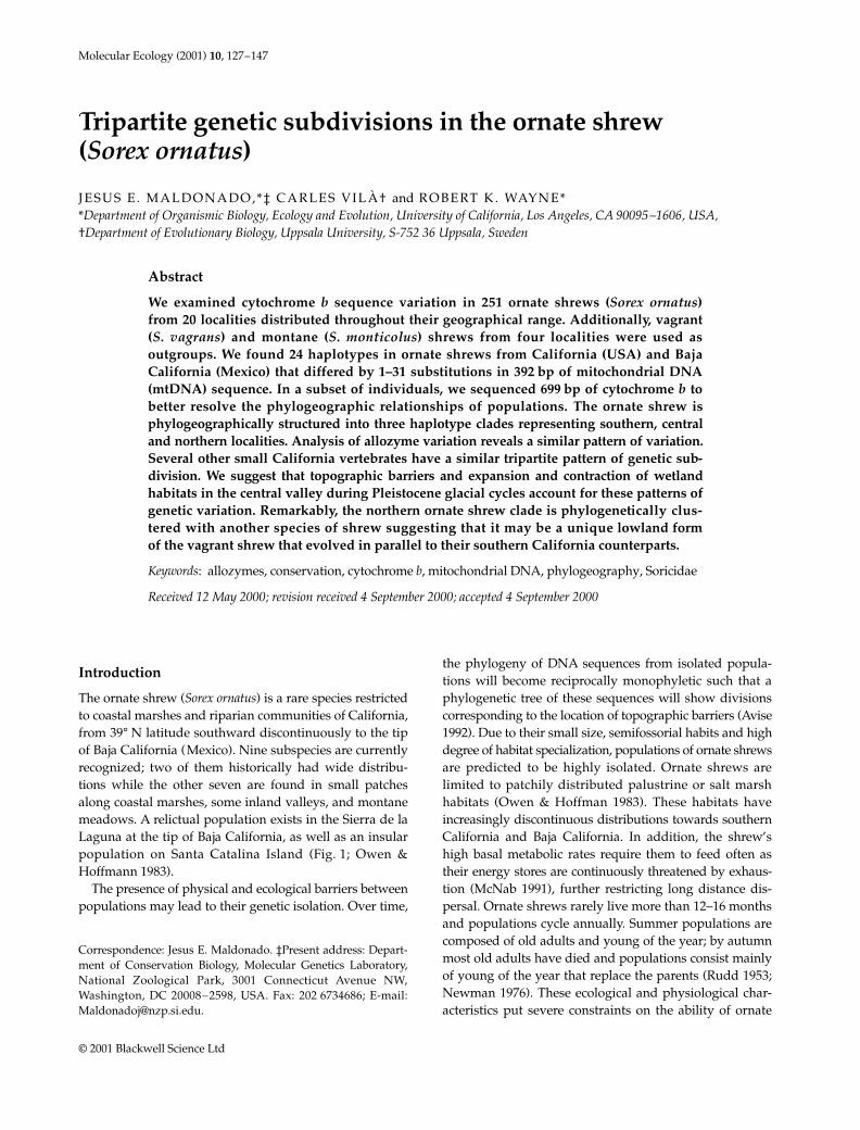
Fig. 1 Location of the 24 sampled shrew populations in theSouth-western US and North-western Mexico (Table 1). Circlesindicate sampling localities for Sorex ornatus, squares aresampling localities for S. vagrans and/or S. monticolus. Thedistribution of the nine subspecies of ornate shrew (S. ornatus)are indicated (adapted from Owen & Hoffman 1983). Thedistribution of S. vagrans in Nevada and California (adaptedfrom Hall 1981) is also shown. Genetic discontinuities areindicated by transverse thick lines (see text).
MEC1178.fm Page 128 Friday, December 8, 2000 3:38 PM

G E N E T I C S U B D I V I S I O N I N O R N AT E S H R E W S
129
© 2001 Blackwell Science Ltd,
Molecular Ecology
, 10, 127–147
localities where vagrant and ornate shrews have beenfound together are in the Sierra Nevada and in marshesaround the San Francisco Bay area. Samples from montaneshrews from two different localities and vagrant shrewsfrom four different localities, including areas of sympatry,were included in the study (see Table 1 and Fig. 1) andwere used as outgroups in the phylogenetic analysis.
DNA extraction, polymerase chain reaction amplification and sequencing
Tissue samples (50 mg or 100
µ
L) were transferred to1.7 mL eppendorf tubes containing 500
µ
L of 1
×
TNEpH 8.0. Genomic DNA was isolated by proteinase Kdigestion, followed by extraction with phenol/chloroform/isoamyl alcohol, precipitated with ethanol and resuspendedin TE pH 8.0 to yield a final concentration of about 1
µ
g/
µ
L(Sambrook
et al
. 1989). Four universal primers (H15149,Kocher
et al
. 1989; L14724, Meyer & Wilson 1990; H15915and L15513, Irwin
et al
. 1991) were used to amplify 425 bpand 402 bp of the mitochondrial cytochrome
b
gene. Each
polymerase chain reaction (PCR) reaction mixture containedapproximately 100 ng of genomic DNA, 25 pmoles ofeach primer and 1 m
m
dNTP mix in a reaction bufferincluding 50 m
m
KCl, 2.5 m
m
MgCl
2
, 10 m
m
Tris-HCl(pH 8.8), and 2.5 U of
Taq
DNA polymerase in a totalvolume of 50
µ
L. Forty cycles of amplification were run ina programmable Perkin-Elmer Cetus DNA thermal cyclermodel 480 as follows: denaturation at 94
°
C for 45 s,annealing at 60
°
C for 30 s, and extension at 72
°
C for 45 s.The double-stranded products were separated in a 2%Nusieve (FMC Corporation, Rockland, MD) agarose gelin TAE buffer and stained with ethidium bromide. Theappropriate band was excised, then purified using aGeneclean Kit (BIO 101).
Direct sequencing of double-stranded DNA wascarried out using modifications of DMSO-based pro-tocols (Green
et al
. 1989; Winship 1989) and a SequenaseVersion 2.0 kit (US Biochemicals) labelling nucleotideswith
35
S. The sequencing reaction products were separatedby electrophoresis in a 6% polyacrylamide gel for 3 h at55 W in a Stratagene Base Ace Sequencing apparatus. The
Table 1 Subspecies, sampling locality and sample size used in the mtDNA and allozyme analyses for Sorex ornatus, S. vagrans andS. monticolus. Locality codes correspond to localities in Fig. 1
Local.code Subspecies Locality County State
mtDNA(n)
Allozyme(n)
Ornate shrews1 Sorex ornatus (unamed) Dye Creek Ranch Tehema California 7 —2 S. o. sinuosus Grizzly Island Solano California 8 83 S. o. californicus Rush Ranch Solano California 6 84 S. o. californicus El Portal, Sierra Nevada Mariposa California 9 95 S. o. californicus Los Banos Wildlife Area Merced California 14 146 S. o. salarius Mouth of the Salinas River Monterey California 16 167 S. o. relictus Kern Lake Preserve Kern California 17 108 S. o. salicornicus Point Mugu Ventura California 3 —9 S. o. salicornicus Rancho Palos Verdes Los Angeles California 3 3
10 S. o. salicornicus Bolsa Chica State Beach Orange California 1 —11 S. o. willetti Catalina Island Los Angeles California 3 —12 S. o. ornatus Kern River, Sierra Nevada Kern California 14 —13 S. o. ornatus Vandenburg Air Force Base Santa Barbara California 13 1214 S. o. ornatus Bluff lake, San Bernardino Mts. San Bernardino California 15 1015 S. o. ornatus James Reserve, San Jacinto Mts. Riverside California 3 —16 S. o. ornatus Camp Pendleton U.S.M.C. San Diego California 12 —17 S. o. ornatus Torrey Pines State Reserve San Diego California 36 —18 S. o. ornatus Mouth of El Rosario River — Baja California 5 519 S. o. ornatus San Pedro Mts. — Baja California 10 —20 S. o. lagunae Sierra de la Laguna Mts. — Baja California 11 11
Wandering shrews21 S. v. vagrans Bodega Bay Sonoma California 21 1322 S. v. vagrans Sweetwater Mts. Mono California 2 —23 S. v. vagrans Shasta Mt. Shasta California 2 —24 S. v. vagrans Jarbridge Mts. Elko Nevada 1 —
Montane Shrews22 S. m. monticolus Sweetwater Mts Mono California 1 —23 S. m. monticolus Shasta Mt Shasta California 1 —
MEC1178.fm Page 129 Friday, December 8, 2000 3:38 PM
130
J . E . M A L D O N A D O , C . V I L À and R . K . WAY N E
© 2001 Blackwell Science Ltd,
Molecular Ecology
, 10, 127–147
gels were then dried and exposed to autoradiographicfilm (Kodak Biomax) for 1–3 days. Sequence films werescored on an IBI gel reader, and entered into the MacVectorcomputer program (IBI-Kodak). Sequences of bothstrands were obtained for 392 bp within the left domainof the cytochrome
b
. An additional 307 bp fragment(amplified with the primers L15513 and H15915) wassequenced from both strands of the right domain of thecytochrome
b
for representative taxa from each cladeto provide better support for putative groupings of shrewhaplotypes. Sequences were aligned first by eye, then byusing Clustal V (Higgins & Sharp 1989), and recheckedby eye. Sequence data have been submitted to GenBank(accession numbers: AF300652–AF300699).
After we sequenced a representative sample of 1–5individuals from each locality for the 392 bp segment ofcytochrome
b
, we typed the additional samples from eachpopulation by single-stranded conformation polymorph-ism analysis (SSCP, Lessa & Applebaum 1993; Girman1996). SSCP is a very sensitive method for detectingmutations in short DNA segments and was utilized toscreen shrew samples from each population to determinethe number of different haplotypes. However, becauseSSCP is most sensitive if fragments are less than 300 bp,an internal primer was designed at position L14841 (Kocher
et al
. 1989) and used in conjunction with the universalprimer H15149. These primers amplify a 308-bp fragment,including the most variable area determined from thesequencing of the entire 392 bp fragment. Primers wereend-labelled with [
γ
32
P]-ATP in a 25-
µ
L polynucleotidekinase reaction. The end-labelled primers were thenincluded in a PCR reaction identical to that above and theproducts were run in a nondenaturing gel. Haplotypestandards representing each cytochrome
b
region sequencefound in the initial survey were included on every gel.We typed a total of 232 individuals. New haplotypesidentified using SSCP analyses were sequenced as explainedabove.
Sequence analysis
The cytochrome
b
sequence data from the two regionstotalled 699 bp and were analysed using three phylogeneticmethods: maximum parsimony, maximum likelihood,and neighbour-joining. To determine the most parsimonioustree, we used unweighted maximum parsimony with thebranch-and-bound option of
paup
version 3.1.1 (Swofford1993). Confidence in estimated relationships was deter-mined using 1000 bootstrap pseudoreplicates (Felsenstein1985). Maximum-likelihood trees were constructed usingthe
phylip
program version 3.2 (Felsenstein 1989). For theseanalyses we used the empirically determined frequenciesof nucleotides and an average transition/transversionratio determined by pairwise comparisons of all taxa.
Finally, the genetic distance between haplotypes wasestimated by the Kimura 2-parameter model (Kimura1981) and used to calculate a neighbour-joining tree (Saitou& Nei 1987).
We used
amova
(analysis of molecular variance) todeduce the significance of geographical divisions amonglocal and regional population groupings (Excoffier
et al
.1992).
amova
is a hierarchical approach analogous toanalysis of variance (
anova
) in which haplotype distancescompared at various hierarchical levels are used as
F
-statistic analogs, designated as
φ
statistics. Gene flowwithin and among regions was approximated as
N
F
m
F
,the number of female migrants between population pergeneration, and was estimated using the expression
F
ST
= 1/(1 + 2
N
F
m
F
) where
N
F
is the female effective popu-lation size and
m
F
is the female migration rate (Slatkin1987, 1993; Baker
et al
. 1994). We used pairwise estimatesof
φ
ST
as surrogates for
F
ST
among regional groupings ofpopulations (e.g. Stanley
et al
. 1996). Following Slatkin(1993), we assessed differentiation by distance by plottingpairwise genetic distance values against geographicaldistance. The significance of the association betweenthe two distance matrices was determined with a Mantelpermutation test (Mantel 1967). A significant associationbetween genetic distance and geographical distanceindicates genetic structuring in populations and suggeststhat dispersal of individuals is limited (Slatkin 1993).We used the Arlequin 1.1 (Schneider
et al
. 1997) programto perform
amova
as well as Fisher’s exact test of popula-tion differentiation as described in Raymond & Rousset(1995). The
dna
sp program (version 2.93, Rozas & Rozas1997) was used to calculate the likelihood ratio test oflinkage disequilibrium (Hill & Robertson 1968) and Tajima’stest of selective neutrality (Tajima 1989).
Allozyme electrophoresis
A subset of the samples used for mtDNA analysis wasanalysed for allozyme variation (Table 1). Only populationsfor which we could obtain permits to sample more thanfive animals and extract heart, liver and kidney sampleswere studied. Extracted samples were stored at –70
°
Cuntil processed. Tissue preparation, horizontal starch-gelelectrophoresis, and biochemical stain procedures modifiedfrom techniques described by Selander
et al
. (1971) andGeorge (1988) were used to type samples (Appendix 1).Thirty presumptive loci were scored (George 1988; Collins& George 1990). Allelic frequencies, direct-count estimatesof mean heterozygosity (
H
), and percentage of polymorphicloci (P) were calculated for each population using
biosys
-1(Swofford & Selander 1981). Each locus was tested todetermine conformance with Hardy–Weinberg expecta-tions. Cluster analyses were performed using Rogers’distance (Rogers 1972) and the Wagner procedure (Farris
MEC1178.fm Page 130 Friday, December 8, 2000 3:38 PM
G E N E T I C S U B D I V I S I O N I N O R N AT E S H R E W S
131
© 2001 Blackwell Science Ltd,
Molecular Ecology
, 10, 127–147
1970). Wright’s
F
ST
was calculated and used to estimatethe number of migrants among populations using theexpression, for diploid data,
FST = 1/(1 + 4Nm) (Wright1969, 1978). Finally, we tested for gametic disequilibriumbetween all pairs of allozyme loci and between allozymeloci and mitochondrial haplotypes using a likelihoodratio test with an empirical distribution of disequilibriumvalues determined by permutation (Slatkin & Excoffier1996). The Arlequin program version 1.1 was used forthese calculations.
To assess the likelihood of finding one of the observedgenotypes in each population or clade grouping we usedan assignment test (Paetkau et al. 1995; Waser & Strobeck1998). This approach calculates the likelihood of findingan individual genotype in a defined population groupingand assigns it to the population with the highest likeli-hood. The degree of differentiation between regions canbe characterized by the percentage of correct assignments(Paetkau et al. 1995). Finally, the proportion of sharedalleles between pairs of individuals was used to build adistance matrix. We used the distance dij = −ln(Pij), wherePij is the proportion of shared alleles between individualsi and j. This distance matrix was calculated using theprogram microsat (http://human.stanford.edu/microsat)and was used to construct a neighbour-joining tree ofindividuals.
Results
Sequence variation
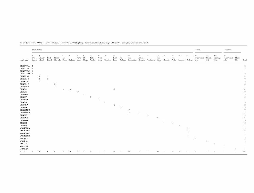
We found 24 different haplotypes in ornate shrews. Exceptfor three population groupings (Grizzly Island with RushRanch; James Reserve with San Bernardino, Los Banoswith Salinas and Kern River), all populations had uniquehaplotypes (Table 2). In addition, the Sorex vagrans samplesthat were obtained from four different localities (BodegaBay, Sweetwater Mountains, Mount Shasta, and JarbridgeMountains) had seven different haplotypes and twoS. monticolus from different localities (Sweetwater Mountainsand Mount Shasta) had different haplotypes.
The cytochrome b gene of ornate shrews is one of themost polymorphic in mammals (Irwin et al. 1991; Smith& Patton 1993; Lara et al. 1996; Lessa & Cook 1998). Inornate shrews, we found 36 variable sites in the 392 bpcytochrome b fragment, 33 of which were transitions andthree were transversions. Sixty-two positions varied acrossthe 392 bp cytochrome b fragment in comparisons of ornateshrews to S. vagrans and S. monticolus. Fifty-seven of thesewere phylogenetically informative, 50 were transitionsand seven were transversions. A total of 99 substitutionswere observed over all pairwise comparisons; 14 occurredat first codon positions, seven at second positions, and 78at third positions. Additionally, we sequenced 307 bp from
the left domain of the cytochrome b gene sequenced in 16shrews, including representatives of ornate shrews fromeach sequence clade defined in preliminary trees basedon shorter sequences (Fig. 2a). In the combined 699 bpfragment, 109 variable sites were observed that distin-guished sequences of the ornate, vagrant and montaneshrews, 69 of which were phylogenetically informative.Of 139 substitutions observed in pairwise comparisons ofsequences, 126 were transitions and 13 were transversions.Consequently, the transition to transversion ratio was 10.3.Twenty-three changes occurred at first codon positions,seven at second positions, and 109 at third positions.
Considering the complete 699 bp sequence, the meandivergence between the montane shrew sequence andtwo vagrant shrew sequences was 9.5% (9.5–9.6%) andbetween the montane shrew and 12 ornate shrew haplo-types it was 9.9% (SD = 0.6; range: 9.0–10.8%, n = 12). Thedivergence between vagrant and ornate shrew haplotypeswas 5.3% (SD = 1.8, range: 1.2–7.3, n = 24), significantlylower than the divergence observed between montaneand ornate shrews (Mann–Whitney’s U = 288, P < 0.001).The range of the divergence observed between vagrantand ornate shrew haplotypes is almost identical to thatobserved between ornate sequences (range: 0.3–7.2%),however, the mean divergence is lower between ornatesequences (3.0%, SD = 2.0, U = 341, P < 0.001). Consequently,montane shrews have cytochrome b sequences highlydivergent from those in ornate and vagrant shrews, whereasthe latter two species are genetically similar.
Phylogeography of haplotypes
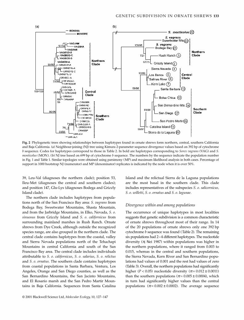
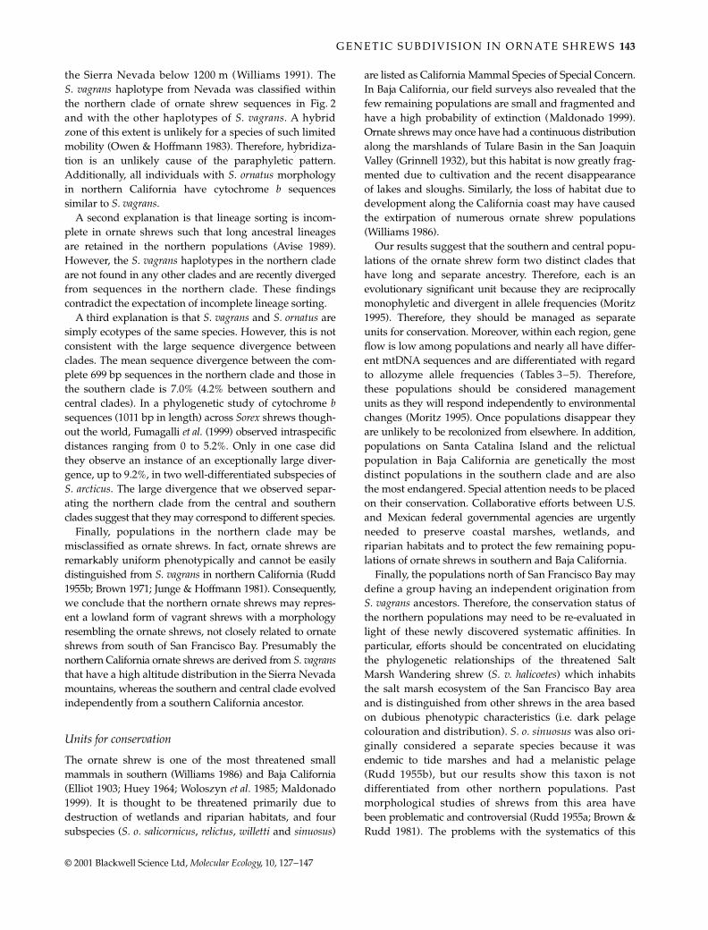
We found three distinct geographical clades in phylo-genetic trees based on the 392 bp fragment in all samplesand 699 bp sequences based on a reduced subset of 16individuals (Fig. 2). These clades generally were supportedin more than 80%, and 90%, of bootstrapped trees basedon short and long sequences, respectively (Fig. 2). Withineach clade, the topology varies among tree buildingmethods, few nodes were supported in more than 50%of the bootstrap iterations and no support was evidentfor the subspecies that are distributed in several of thesampled populations (see, for example, the lack of supportfor a common origin of haplotypes ORNPTM, ORNSPVand ORNBCH, the haplotypes observed in populationsattributed to S. o. salicornicus). However, in the northernclade, S. vagrans from higher elevations (Mount Shasta,Sweetwater Mountains and Jarbridge Mountains) formeda well-supported group (94% and 97% bootstrap valuesin the parsimony and neighbour-joining trees, respectively).Comparison of the 232 amino acids translated from thecomplete 699 bp sequence between the three ornatus cladesshows that four amino acid changes were unambiguous:position 16, Asn-Ser (diagnoses the central clade); position
MEC1178.fm Page 131 Friday, December 8, 2000 3:38 PM
132J. E
. MA
LD
ON
AD
O, C
. VIL
À and
R. K
. WA
YN
E
© 2001 B
lackwell Science L
td, M
olecular Ecology, 10, 127–147
Table 2 Sorex ornatus (ORN), S. vagrans (VAG) and S. monticolus (MON) haplotype distribution at the 24 sampling localities in California, Baja California and Nevada
Sorex ornatus S. mont. S. vagrans
Haplotype
1Dye Creek
2 Grizzly Island
3 Rush Ranch
4 Sierra Nevada
5 Los Banos
6
Salinas
7 Kern Lake
8 Pt Mugu
9 Palos Verdes
10 Bolsa Chica
11
Catalina
12 Kern River
13 Sta Barbara
14 San Bernardino
15 James Reserve
16
Pendleton
17 San Diego
18
Rosario
19 San Pedro
20
Laguna
21
Bodega
22 Sweetwater Mts.
23 Shasta Mt.
24 Jarbridge Mts.
22 Sweetwater Mts.
23 Shasta Mt. Total
ORNDYE-A 2 2ORNDYE-B 2 2ORNDYE-C 1 1ORNDYE-D 2 2ORNSGI-A 3 1 4ORNSGI-B 4 3 7ORNSGI-C 1 2 3ORNSIN-A 8 8ORNSIN-B 1 1ORNSAL 14 16 12 42ORNSKL 17 17ORNPTM 3 3ORNSPV 3 3ORNBCH 1 1ORNSCI 3 3ORNKRP 2 2ORNSBR 13 13ORNSBM-B 7 7ORNSBM-A 8 3 11ORNPEN 12 12ORNSND 36 36ORNROS 5 5ORNSSP 10 10ORNSLA 11 11VAGBOD-A 12 12VAGBOD-B 7 7VAGBOD-C 1 1VAGBOD-D 1 1VAGSWE 2 2VAGSHA 2 2VAGJAM 1 1MONSWE 1 1MONSHA 1 1TOTAL 7 8 6 9 14 16 17 3 3 1 3 14 13 15 3 12 36 5 10 11 21 2 2 1 1 1 234
ME
C1178.fm
Page 132 F
riday, Decem
ber 8, 2000 3:38 PM
G E N E T I C S U B D I V I S I O N I N O R N AT E S H R E W S 133
© 2001 Blackwell Science Ltd, Molecular Ecology, 10, 127–147
39, Leu-Val (diagnoses the northern clade); position 53,Ileu-Met (diagnoses the central and southern clades);and position 147, Glu-Lys (diagnoses Bodega and GrizzlyIsland clade).
The northern clade includes haplotypes from popula-tions north of the San Francisco Bay area: S. vagrans fromBodega Bay, Sweetwater Mountains, Shasta Mountain,and from the Jarbridge Mountains, in Elko, Nevada, S. o.sinuosus from Grizzly Island and S. o. californicus fromsurrounding mainland marshes in Rush Ranch. Ornateshrews from Dye Creek, although outside the recognizedspecies range, are also grouped in the northern clade. Thecentral clade contains haplotypes from the coastal, valleyand Sierra Nevada populations north of the TehachapiMountains in central California and south of the SanFrancisco Bay area. The central clade includes individualsattributable to S. o. californicus, S. o. salarius, S. o. relictusand S. o. ornatus. The southern clade contains haplotypesfrom coastal populations in Santa Barbara, Ventura, LosAngeles, Orange and San Diego counties, as well as theSan Bernardino Mountains, the San Jacinto Mountains,and El Rosario marsh and the San Pedro Martir Moun-tains in Baja California. Sequences from Santa Catalina
Island and the relictual Sierra de la Laguna populationsare the most basal in the southern clade. This cladeincludes representatives of the subspecies S. o. salicornicus,S. o. willetti, S. o. ornatus and S. o. lagunae.
Divergence within and among populations
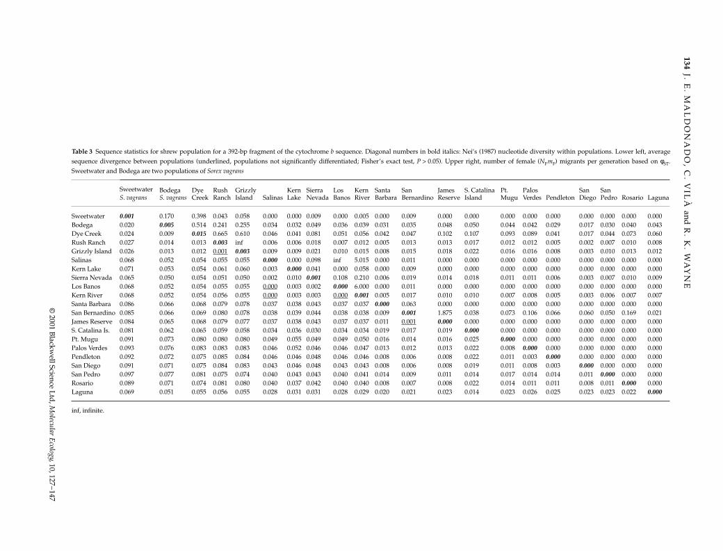
The occurrence of unique haplotypes in most localitiessuggests that genetic subdivision is a common characteristicof ornate shrews throughout most of their range. In 14of the 20 populations of ornate shrews only one 392 bpcytochrome b sequence was found (Table 2). The remainingsix populations had 2–4 different haplotypes. The nucleotidediversity (π, Νei 1987) within populations was higher inthe northern populations, where it ranged from 0.003 to0.015, whereas in the central and southern populations,the Sierra Nevada, Kern River and San Bernardino popu-lations had values of 0.001 and the rest had values of zero(Table 3). Overall, the northern populations had significantlyhigher (P < 0.05) nucleotide diversity (π = 0.012 ± 0.0011)than the southern populations (π = 0.005 ± 0.0004), whichin turn had significantly higher values than the centralpopulations (π = 0.002 ± 0.0002). The average sequence
Fig. 2 Phylogenetic trees showing relationships between haplotypes found in ornate shrews form northern, central, southern Californiaand Baja California. (a) Neighbour-joining (NJ) tree using Kimura 2-parameter sequence divergence values based on 392 bp of cytochromeb sequence. Codes for haplotypes correspond to those in Table 2. In bold are haplotypes corresponding to Sorex vagrans (VAG) and S.monticolus (MON). (b) NJ tree based on 699 bp of cytochrome b sequence. The numbers by the sequence indicate the population numberin Fig. 1 and Table 1. Similar topologies were obtained using parsimony (MP) and maximum likelihood analysis in both cases. Percentage ofsupport in 1000 bootstrap NJ (numerator) and MP (denominator) replicates is indicated by the node when it is over 50%.
MEC1178.fm Page 133 Friday, December 8, 2000 3:38 PM
134J. E
. MA
LD
ON
AD
O, C
. VIL
À and
R. K
. WA
YN
E
© 2001 B
lackwell Science L
td, M
olecular Ecology, 10, 127–147
Table 3 Sequence statistics for shrew population for a 392-bp fragment of the cytochrome b sequence. Diagonal numbers in bold italics: Nei’s (1987) nucleotide diversity within populations. Lower left, averagesequence divergence between populations (underlined, populations not significantly differentiated; Fisher’s exact test, P > 0.05). Upper right, number of female (NFmF) migrants per generation based on φST.Sweetwater and Bodega are two populations of Sorex vagrans
Sweetwater S. vagrans
Bodega S. vagrans
Dye Creek
Rush Ranch
Grizzly Island Salinas
Kern Lake
Sierra Nevada
Los Banos
Kern River
Santa Barbara
San Bernardino
James Reserve
S. Catalina Island
Pt. Mugu
Palos Verdes Pendleton
San Diego
San Pedro Rosario Laguna
Sweetwater 0.001 0.170 0.398 0.043 0.058 0.000 0.000 0.009 0.000 0.005 0.000 0.009 0.000 0.000 0.000 0.000 0.000 0.000 0.000 0.000 0.000Bodega 0.020 0.005 0.514 0.241 0.255 0.034 0.032 0.049 0.036 0.039 0.031 0.035 0.048 0.050 0.044 0.042 0.029 0.017 0.030 0.040 0.043Dye Creek 0.024 0.009 0.015 0.665 0.610 0.046 0.041 0.081 0.051 0.056 0.042 0.047 0.102 0.107 0.093 0.089 0.041 0.017 0.044 0.073 0.060Rush Ranch 0.027 0.014 0.013 0.003 inf 0.006 0.006 0.018 0.007 0.012 0.005 0.013 0.013 0.017 0.012 0.012 0.005 0.002 0.007 0.010 0.008Grizzly Island 0.026 0.013 0.012 0.001 0.003 0.009 0.009 0.021 0.010 0.015 0.008 0.015 0.018 0.022 0.016 0.016 0.008 0.003 0.010 0.013 0.012Salinas 0.068 0.052 0.054 0.055 0.055 0.000 0.000 0.098 inf 5.015 0.000 0.011 0.000 0.000 0.000 0.000 0.000 0.000 0.000 0.000 0.000Kern Lake 0.071 0.053 0.054 0.061 0.060 0.003 0.000 0.041 0.000 0.058 0.000 0.009 0.000 0.000 0.000 0.000 0.000 0.000 0.000 0.000 0.000Sierra Nevada 0.065 0.050 0.054 0.051 0.050 0.002 0.010 0.001 0.108 0.210 0.006 0.019 0.014 0.018 0.011 0.011 0.006 0.003 0.007 0.010 0.009Los Banos 0.068 0.052 0.054 0.055 0.055 0.000 0.003 0.002 0.000 6.000 0.000 0.011 0.000 0.000 0.000 0.000 0.000 0.000 0.000 0.000 0.000Kern River 0.068 0.052 0.054 0.056 0.055 0.000 0.003 0.003 0.000 0.001 0.005 0.017 0.010 0.010 0.007 0.008 0.005 0.003 0.006 0.007 0.007Santa Barbara 0.086 0.066 0.068 0.079 0.078 0.037 0.038 0.043 0.037 0.037 0.000 0.063 0.000 0.000 0.000 0.000 0.000 0.000 0.000 0.000 0.000San Bernardino 0.085 0.066 0.069 0.080 0.078 0.038 0.039 0.044 0.038 0.038 0.009 0.001 1.875 0.038 0.073 0.106 0.066 0.060 0.050 0.169 0.021James Reserve 0.084 0.065 0.068 0.079 0.077 0.037 0.038 0.043 0.037 0.037 0.011 0.001 0.000 0.000 0.000 0.000 0.000 0.000 0.000 0.000 0.000S. Catalina Is. 0.081 0.062 0.065 0.059 0.058 0.034 0.036 0.030 0.034 0.034 0.019 0.017 0.019 0.000 0.000 0.000 0.000 0.000 0.000 0.000 0.000Pt. Mugu 0.091 0.073 0.080 0.080 0.080 0.049 0.055 0.049 0.049 0.050 0.016 0.014 0.016 0.025 0.000 0.000 0.000 0.000 0.000 0.000 0.000Palos Verdes 0.093 0.076 0.083 0.083 0.083 0.046 0.052 0.046 0.046 0.047 0.013 0.012 0.013 0.022 0.008 0.000 0.000 0.000 0.000 0.000 0.000Pendleton 0.092 0.072 0.075 0.085 0.084 0.046 0.046 0.048 0.046 0.046 0.008 0.006 0.008 0.022 0.011 0.003 0.000 0.000 0.000 0.000 0.000San Diego 0.091 0.071 0.075 0.084 0.083 0.043 0.046 0.048 0.043 0.043 0.008 0.006 0.008 0.019 0.011 0.008 0.003 0.000 0.000 0.000 0.000San Pedro 0.097 0.077 0.081 0.075 0.074 0.040 0.043 0.043 0.040 0.041 0.014 0.009 0.011 0.014 0.017 0.014 0.014 0.011 0.000 0.000 0.000Rosario 0.089 0.071 0.074 0.081 0.080 0.040 0.037 0.042 0.040 0.040 0.008 0.007 0.008 0.022 0.014 0.011 0.011 0.008 0.011 0.000 0.000Laguna 0.069 0.051 0.055 0.056 0.055 0.028 0.031 0.031 0.028 0.029 0.020 0.021 0.023 0.014 0.023 0.026 0.025 0.023 0.023 0.022 0.000
inf, infinite.
ME
C1178.fm
Page 134 F
riday, Decem
ber 8, 2000 3:38 PM
G E N E T I C S U B D I V I S I O N I N O R N AT E S H R E W S 135
© 2001 Blackwell Science Ltd, Molecular Ecology, 10, 127–147
divergence between different populations of S. ornatusranged from 0.1% to 8.5% (Table 3). The maximum is alarge value compared with that found in other mammalspecies (Taberlet et al. 1998). Average sequence divergencebetween regions ranged from 4.11% ± 0.90 (southern vs.central) to 7.59 ± 0.15 (northern vs. southern).
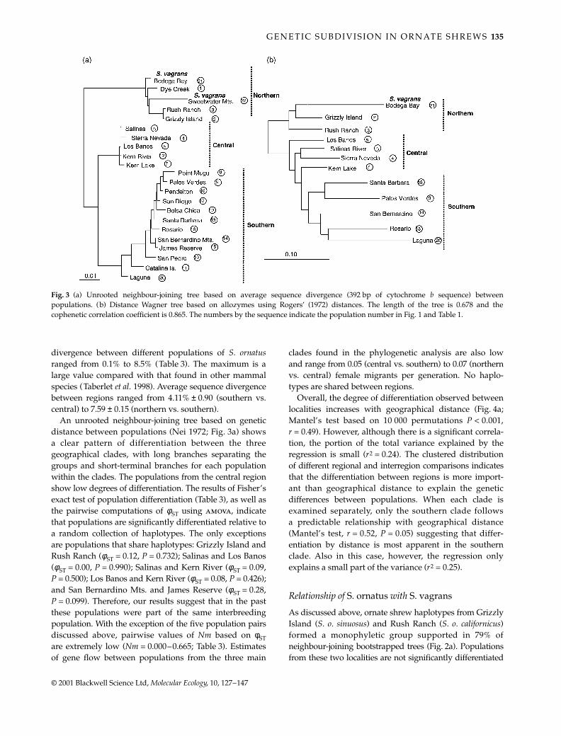
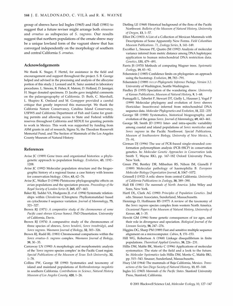
An unrooted neighbour-joining tree based on geneticdistance between populations (Nei 1972; Fig. 3a) showsa clear pattern of differentiation between the threegeographical clades, with long branches separating thegroups and short-terminal branches for each populationwithin the clades. The populations from the central regionshow low degrees of differentiation. The results of Fisher’sexact test of population differentiation (Table 3), as well asthe pairwise computations of φST using amova, indicatethat populations are significantly differentiated relative toa random collection of haplotypes. The only exceptionsare populations that share haplotypes: Grizzly Island andRush Ranch (φST = 0.12, P = 0.732); Salinas and Los Banos(φST = 0.00, P = 0.990); Salinas and Kern River (φST = 0.09,P = 0.500); Los Banos and Kern River (φST = 0.08, P = 0.426);and San Bernardino Mts. and James Reserve (φST = 0.28,P = 0.099). Therefore, our results suggest that in the pastthese populations were part of the same interbreedingpopulation. With the exception of the five population pairsdiscussed above, pairwise values of Nm based on φSTare extremely low (Nm = 0.000–0.665; Table 3). Estimatesof gene flow between populations from the three main
clades found in the phylogenetic analysis are also lowand range from 0.05 (central vs. southern) to 0.07 (northernvs. central) female migrants per generation. No haplo-types are shared between regions.
Overall, the degree of differentiation observed betweenlocalities increases with geographical distance (Fig. 4a;Mantel’s test based on 10 000 permutations P < 0.001,r = 0.49). However, although there is a significant correla-tion, the portion of the total variance explained by theregression is small (r2 = 0.24). The clustered distributionof different regional and interregion comparisons indicatesthat the differentiation between regions is more import-ant than geographical distance to explain the geneticdifferences between populations. When each clade isexamined separately, only the southern clade followsa predictable relationship with geographical distance(Mantel’s test, r = 0.52, P = 0.05) suggesting that differ-entiation by distance is most apparent in the southernclade. Also in this case, however, the regression onlyexplains a small part of the variance (r2 = 0.25).
Relationship of S. ornatus with S. vagrans
As discussed above, ornate shrew haplotypes from GrizzlyIsland (S. o. sinuosus) and Rush Ranch (S. o. californicus)formed a monophyletic group supported in 79% ofneighbour-joining bootstrapped trees (Fig. 2a). Populationsfrom these two localities are not significantly differentiated
Fig. 3 (a) Unrooted neighbour-joining tree based on average sequence divergence (392 bp of cytochrome b sequence) betweenpopulations. (b) Distance Wagner tree based on allozymes using Rogers’ (1972) distances. The length of the tree is 0.678 and thecophenetic correlation coefficient is 0.865. The numbers by the sequence indicate the population number in Fig. 1 and Table 1.
MEC1178.fm Page 135 Friday, December 8, 2000 3:38 PM

136 J . E . M A L D O N A D O , C . V I L À and R . K . WAY N E
© 2001 Blackwell Science Ltd, Molecular Ecology, 10, 127–147
(Table 3) and have all haplotypes in common, implyingthat they are part of the same interbreeding population.Ornate shrew haplotypes from Grizzly Island, Rush Ranchand Dye Creek localities are grouped with those attributableto S. vagrans from Bodega Bay, Sweetwater Mountains,Mt. Shasta, and Jarbridge Mountains (Elko Co., Nevada)to form the northern clade of haplotypes (Fig. 2, Fig. 3).S. vagrans haplotypes from higher elevations formed amonophyletic group, which was supported in 94% and97% of bootstrapped trees in maximum parsimony andneighbour-joining trees (Fig. 2), and differed by 2 (0.6%)
to 4 (1.2%) substitutions from each other and 6 (1.5%) to11 (3.6%) from haplotypes in the other populations in thenorthern clade. Consequently, the ornate shrew fromnorthern California is a paraphyletic group that includeshaplotypes from a related species.
Divergence time inferred from sequence data
The cytochrome b sequence data can be used to estimatedivergence time of the three major ornate shrew cladeswhen corrected for ancestral polymorphism within species(Nei 1987; Avise & Walker 1998; but see Hillis et al. 1996).The net sequence divergence between southern and centralclades is 4.2%, and assuming a mutation rate of 2% permillion years (Myr) (Wilson et al. 1985; the divergencerate would thus be about 4% per Myr if the sequences arefar from saturation), the two clades diverged about 1.1million years ago (Ma). Similarly, the southern and northernclades have a net sequence divergence of 4.9%, whichimplies a divergence time of approximately 1.2 Ma. Thenet sequence divergence between S. monticolus and theingroup species is 6.5%, implying a divergence time of 1.6Myr. Saturation was not evident in saturation plots ofgenetic distances vs. number of substitutions, and Tajima’stest of selective neutrality (Kimura 1983) showed no signi-ficant rate differences (P > 0.10) among and within clades.Finally, the mean divergence between sequences withinclades is 1.7%, 0.6% and 1.3% for northern, central andsouthern clades, respectively. These values correspond todivergence times of 0.425, 0.150 and 0.325 Ma. The lowermean divergence in the central clade suggests a morerecent radiation of haplotypes.
Allozymic variation
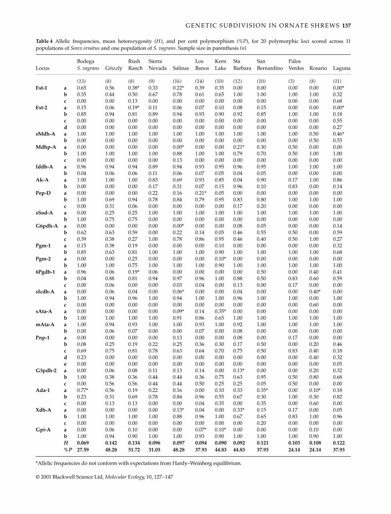
Of the 30 loci examined, 10 were fixed for a single alleleand 20 were polyallelic in at least one population (Appendix1). Mean heterozygosity (H) within populations rangedfrom 0.069 to 0.142 (Table 4) (mean across all samples,0.105) and falls within the values reported for soricids(Tolliver et al. 1985). On average, heterozygosity wassignificantly higher in northern populations (0.115 ± 0.040)than in central populations (0.094 ± 0.003) (Chi-squaretest; P < 0.05), but did not differ significantly from thesouthern populations (0.109 ± 0.01). Polymorphism withinpopulations varied from 24.14 to 51.72% and was highestin northern populations (mean 42.53 ± 13.05) and lowestin the southern populations (mean 33.79 ± 9.25), althoughnot statistically significant (Chi-square test; P = 0.59).Overall, no linkage disequilibrium was detected (maximum-likelihood ratio test with Bonferroni correction for multiplecomparisons, P > 0.05).
Geographic patterns of variation are evident for a fewloci. For example, the Est-2 allele ‘a’ occurs at high
Fig. 4 Scatterplots showing the relationship between geographicaldistance and genetic distance between populations. (a) Resultsbased on genetic distances (Nei 1972) derived from mtDNA ana-lysis of 22 populations. Regression statistics: y = –0.039 + 0.013(x),r2 = 0.24. (b) Results based on genetic distances (Rogers 1972)derived from allozyme analysis of 11 populations. Regressionstatistics: y = –0.023 + 0.026(x), r2 = 0.44.
MEC1178.fm Page 136 Friday, December 8, 2000 3:38 PM
G E N E T I C S U B D I V I S I O N I N O R N AT E S H R E W S 137
© 2001 Blackwell Science Ltd, Molecular Ecology, 10, 127–147
Table 4 Allelic frequencies, mean heterozygosity (H ), and per cent polymorphism (%P), for 20 polymorphic loci scored across 11populations of Sorex ornatus and one population of S. vagrans. Sample size in parenthesis (n)
LocusBodega S. vagrans Grizzly
Rush Ranch
Sierra Nevada Salinas
Los Banos
Kern Lake
Sta Barbara
San Bernardino
Palos Verdes Rosario Laguna
(13) (8) (8) (9) (16) (14) (10) (12) (10) (3) (8) (11)Est-1 a 0.65 0.56 0.38* 0.33 0.22* 0.39 0.35 0.00 0.00 0.00 0.00 0.00*
b 0.35 0.44 0.50 0.67 0.78 0.61 0.65 1.00 1.00 1.00 1.00 0.32c 0.00 0.00 0.13 0.00 0.00 0.00 0.00 0.00 0.00 0.00 0.00 0.68
Est-2 a 0.15 0.06 0.19* 0.11 0.06 0.07 0.10 0.08 0.15 0.00 0.00 0.00*b 0.85 0.94 0.81 0.89 0.94 0.93 0.90 0.92 0.85 1.00 1.00 0.18c 0.00 0.00 0.00 0.00 0.00 0.00 0.00 0.00 0.00 0.00 0.00 0.55d 0.00 0.00 0.00 0.00 0.00 0.00 0.00 0.00 0.00 0.00 0.00 0.27
sMdh-A a 1.00 1.00 1.00 1.00 1.00 1.00 1.00 1.00 1.00 1.00 0.50 0.46*b 0.00 0.00 0.00 0.00 0.00 0.00 0.00 0.00 0.00 0.00 0.50 0.55
Mdhp-A a 0.00 0.00 0.00 0.00 0.00* 0.00 0.00 0.21* 0.30 0.50 0.00 0.00b 1.00 1.00 1.00 1.00 0.88 1.00 1.00 0.79 0.70 0.50 1.00 1.00c 0.00 0.00 0.00 0.00 0.13 0.00 0.00 0.00 0.00 0.00 0.00 0.00
Iddh-A a 0.96 0.94 0.94 0.89 0.94 0.93 0.95 0.96 0.95 1.00 1.00 1.00b 0.04 0.06 0.06 0.11 0.06 0.07 0.05 0.04 0.05 0.00 0.00 0.00
Ak-A a 1.00 1.00 1.00 0.83 0.69 0.93 0.85 0.04 0.90 0.17 1.00 0.86b 0.00 0.00 0.00 0.17 0.31 0.07 0.15 0.96 0.10 0.83 0.00 0.14
Pep-D a 0.00 0.00 0.00 0.22 0.16 0.21* 0.05 0.00 0.00 0.00 0.00 0.00b 1.00 0.69 0.94 0.78 0.84 0.79 0.95 0.83 0.80 1.00 1.00 1.00c 0.00 0.31 0.06 0.00 0.00 0.00 0.00 0.17 0.20 0.00 0.00 0.00
sSod-A a 0.00 0.25 0.25 1.00 1.00 1.00 1.00 1.00 1.00 1.00 1.00 1.00b 1.00 0.75 0.75 0.00 0.00 0.00 0.00 0.00 0.00 0.00 0.00 0.00
G6pdh-A a 0.00 0.00 0.00 0.00 0.00* 0.00 0.00 0.08 0.05 0.00 0.00 0.14b 0.62 0.63 0.59 0.00 0.22 0.14 0.05 0.46 0.55 0.50 0.00 0.59c 0.39 0.38 0.27 1.00 0.78 0.86 0.95 0.46 0.40 0.50 1.00 0.27
Pgm-1 a 0.15 0.38 0.19 0.00 0.00 0.00 0.10 0.00 0.00 0.00 0.00 0.32b 0.85 0.63 0.81 1.00 1.00 1.00 0.90 1.00 1.00 1.00 1.00 0.68
Pgm-2 a 0.00 0.00 0.25 0.00 0.00 0.00 0.10* 0.00 0.00 0.00 0.00 0.00b 1.00 1.00 0.75 1.00 1.00 1.00 0.90 1.00 1.00 1.00 1.00 1.00
6Pgdh-1 a 0.96 0.06 0.19* 0.06 0.00 0.00 0.00 0.00 0.50 0.00 0.40 0.41b 0.04 0.88 0.81 0.94 0.97 0.96 1.00 0.88 0.50 0.83 0.60 0.59c 0.00 0.06 0.00 0.00 0.03 0.04 0.00 0.13 0.00 0.17 0.00 0.00
sIcdh-A a 0.00 0.06 0.04 0.00 0.06* 0.00 0.00 0.04 0.00 0.00 0.40* 0.00b 1.00 0.94 0.96 1.00 0.94 1.00 1.00 0.96 1.00 1.00 0.00 1.00c 0.00 0.00 0.00 0.00 0.00 0.00 0.00 0.00 0.00 0.00 0.60 0.00
sAta-A a 0.00 0.00 0.00 0.00 0.09* 0.14 0.35* 0.00 0.00 0.00 0.00 0.00b 1.00 1.00 1.00 1.00 0.91 0.86 0.65 1.00 1.00 1.00 1.00 1.00
mAta-A a 1.00 0.94 0.93 1.00 1.00 0.93 1.00 0.92 1.00 1.00 1.00 1.00b 0.00 0.06 0.07 0.00 0.00 0.07 0.00 0.08 0.00 0.00 0.00 0.00
Pnp-1 a 0.00 0.00 0.00 0.00 0.13 0.00 0.00 0.08 0.00 0.17 0.00 0.00b 0.08 0.25 0.19 0.22 0.25 0.36 0.30 0.17 0.50 0.00 0.20 0.46c 0.69 0.75 0.81 0.78 0.63 0.64 0.70 0.75 0.50 0.83 0.40 0.18d 0.23 0.00 0.00 0.00 0.00 0.00 0.00 0.00 0.00 0.00 0.40 0.32e 0.00 0.00 0.00 0.00 0.00 0.00 0.00 0.00 0.00 0.00 0.00 0.05
G3pdh-2 a 0.00 0.06 0.08 0.11 0.13 0.14 0.00 0.13* 0.00 0.00 0.20 0.32b 1.00 0.38 0.36 0.44 0.44 0.36 0.75 0.63 0.95 0.50 0.80 0.68c 0.00 0.56 0.56 0.44 0.44 0.50 0.25 0.25 0.05 0.50 0.00 0.00
Ada-1 a 0.77* 0.56 0.19 0.22 0.16 0.00 0.10 0.33 0.35* 0.00 0.10* 0.18b 0.23 0.31 0.69 0.78 0.84 0.96 0.55 0.67 0.30 1.00 0.30 0.82c 0.00 0.13 0.13 0.00 0.00 0.04 0.35 0.00 0.35 0.00 0.60 0.00
Xdh-A a 0.00 0.00 0.00 0.00 0.13* 0.04 0.00 0.33* 0.15 0.17 0.00 0.05b 1.00 1.00 1.00 1.00 0.88 0.96 1.00 0.67 0.65 0.83 1.00 0.96c 0.00 0.00 0.00 0.00 0.00 0.00 0.00 0.00 0.20 0.00 0.00 0.00
Gpi-A a 0.00 0.06 0.10 0.00 0.00 0.07* 0.10* 0.00 0.00 0.00 0.10 0.00b 1.00 0.94 0.90 1.00 1.00 0.93 0.90 1.00 1.00 1.00 0.90 1.00H 0.069 0.142 0.134 0.096 0.097 0.094 0.090 0.092 0.121 0.103 0.108 0.122%P 27.59 48.28 51.72 31.03 48.28 37.93 44.83 44.83 37.93 24.14 24.14 37.93
*Allelic frequencies do not conform with expectations from Hardy–Weinberg equilibrium.
MEC1178.fm Page 137 Friday, December 8, 2000 3:38 PM
138 J . E . M A L D O N A D O , C . V I L À and R . K . WAY N E
© 2001 Blackwell Science Ltd, Molecular Ecology, 10, 127–147
frequencies in northern populations, is rare in centralpopulations and is absent from southern populations.Allele ‘b’ for sSod-A occurs at high frequencies in northernpopulations and is absent in central and southern popula-tions. For Pep-D, allele ‘a’ occurs at low frequencies onlyin central populations. Unique alleles were detected infour populations: in Laguna, Est-2 alleles ‘c’ and ‘d’, andPnp-1 allele ‘e’; in Rosario, sIcdh-A allele ‘c’; in Salinas,Mdhp-A allele ‘c’; and in San Bernardino, Xdh-A allele ‘c’.In the latter two populations, the unique alleles were rare(Table 4).
The Wagner method tree (Fig. 3b) has a topology similarto that of upgma and neighbour-joining trees (not shown).There is a strong north to south pattern of clusteringsimilar to that found with the mitochondrial sequencedata. The Wagner method tree shows a northern clusterthat includes populations from Bodega, Grizzly Islandand Rush Ranch and a southern cluster which includesthe populations from southern California and BajaCalifornia. The central populations from Salinas, LosBanos, Sierra Nevada and Kern Lake are sister to thesouthern clade. Some of the highest genetic divergencevalues are found in comparisons with the Laguna andRosario populations as both have unusual allele frequen-cies at four loci (Est-1, Est-2, sMdh-A and Pnp-1; Table 4).
Population differentiation using allozymes
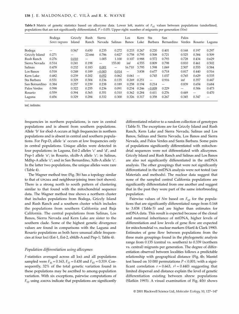
F-statistics averaged across all loci and all populationssampled were FIS = 0.163, FIT = 0.430 and FST = 0.319. Con-sequently, 32% of the total genetic variation found inthese populations may be ascribed to among-populationvariation. With six exceptions, pairwise computations ofFST using amova indicate that populations are significantly
differentiated relative to a random collection of genotypes(Table 5). The exceptions are for Grizzly Island and RushRanch, Kern Lake and Sierra Nevada, Salinas and LosBanos, Salinas and Sierra Nevada, Los Banos and SierraNevada, and Palos Verdes and Santa Barbara. Some pairsof populations significantly differentiated with mitochon-drial sequences were not differentiated with allozymes.Grizzly Island and Rush Ranch and Salinas and Los Banosare also not significantly differentiated in the mtDNAanalysis. The other groupings that were not significantlydifferentiated in the mtDNA analysis were not tested (seeMaterials and methods). The nuclear data suggest thatnone of the sampled central California populations aresignificantly differentiated from one another and suggestthat in the past they were part of the same interbreedingpopulation.
Pairwise values of Nm based on FST for the popula-tions that are significantly differentiated range from 0.168to 3.838 (Table 5) and are higher than estimates formtDNA data. This result is expected because of the clonaland maternal inheritance of mtDNA, higher levels ofdifferentiation and low levels of gene flow are expectedfor mitochondrial vs. nuclear markers (Hartl & Clark 1990).Estimates of gene flow between populations from thethree main groupings found in the phylogenetic analysisrange from 0.135 (central vs. southern) to 0.339 (northernvs. central) migrants per generation. The degree of differ-entiation observed between localities follows a predictablerelationship with geographical distance (Fig. 4b; Manteltest based on 10 000 permutations P < 0.001; with a signi-ficant correlation r = 0.663, r2 = 0.440) suggesting thatlimited dispersal and distance explain the level of geneticdifferentiation existing between shrew populations(Slatkin 1993). A visual examination of Fig. 4(b) shows
Table 5 Matrix of genetic statistics based on allozyme data. Lower left, matrix of FST values between populations (underlined,populations that are not significantly differentiated, P > 0.05). Upper right: number of migrants per generation (Nm)
Bodega Sorex vagrans
Grizzly Island
Rush Ranch
Sierra Nevada Salinas
Los Banos
Kern Lake
Sta Barbara
San Bernardino
Palos Verdes Rosario Laguna
Bodega — 0.567 0.650 0.235 0.272 0.233 0.267 0.220 0.401 0.168 0.197 0.297Grizzly Island 0.271 — 22.666 0.786 0.827 0.758 0.795 0.508 0.721 0.525 0.384 0.509Rush Ranch 0.276 0.010 — 1.005 1.100 0.107 0.988 0.572 0.793 0.728 0.434 0.629Sierra Nevada 0.514 0.241 0.198 — 155.00 inf 4.555 0.809 0.798 0.810 0.461 0.502Salinas 0.478 0.232 0.183 0.001 — 16.710 3.795 1.598 1.069 2.507 0.555 0.584Los Banos 0.518 0.248 0.189 –0.003 0.014 — 3.838 0.677 0.718 0.817 0.440 0.516Kern Lake 0.482 0.239 0.202 0.052 0.062 0.061 — 0.745 1.037 0.765 0.629 0.535Sta Barbara 0.531 0.329 0.304 0.236 0.135 0.269 0.251 — 0.916 inf 0.357 0.447San Bernardino 0.384 0.257 0.239 0.238 0.189 0.258 0.194 0.214 — 0.839 0.654 0.684Palos Verdes 0.598 0.322 0.255 0.236 0.091 0.234 0.246 –0.009 0.229 — 0.306 0.473Rosario 0.559 0.394 0.365 0.351 0.310 0.362 0.284 0.411 0.276 0.449 — 0.470Laguna 0.456 0.329 0.284 0.332 0.300 0.326 0.317 0.358 0.267 0.345 0.347 —
inf, infinite.
MEC1178.fm Page 138 Friday, December 8, 2000 3:38 PM
G E N E T I C S U B D I V I S I O N I N O R N AT E S H R E W S 139
© 2001 Blackwell Science Ltd, Molecular Ecology, 10, 127–147
that the overall trend towards increased genetic distancewith geographical distance is only clear for populationsseparated by less than 750–1000 km. After this point noobvious trend is observed. As with the mtDNA data, wheneach clade is examined separately, only the southerngroup follows a predictable relationship with geographicaldistance (r = 0.778; Mantel’s test P = 0.05). However, thesmall sample size of the central and northern populationslimits the statistical power of permutation tests (Mantel1967). Finally, Roger’s genetic distance between popula-tions based on allozyme data is significantly correlatedwith the corresponding complete cytochrome b sequencedivergence values (Mantel’s test, 10 000 permutations,r = 0.566, P = 0.004).
An assignment test shows that 93% (27/29) of thenorthern shrews are correctly identified as belongingto the northern populations. Two individuals fromGrizzly Island and Rush Ranch are incorrectly assigned tothe southern region. A total of 92% (45/49) of the shrewsfrom the central valley are correctly assigned, and fourindividuals are misassigned (one from Sierra Nevadaand three from Salinas) to the southern populations.Finally, only 83% (34/41) of shrews from the southernpopulations are correctly identified, one individual fromSan Bernardino is assigned to the northern group ofpopulations and six (five from Santa Barbara and onefrom Palos Verdes) are assigned to the central group. Noshrew was wrongly cross-assigned between northern andcentral populations.
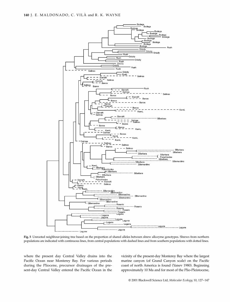
A tree of individuals based on allele sharing distanceshows that in general the three population clades are welldifferentiated (Fig. 5). However, central and southernindividuals are mixed in a portion of the tree. Someindividuals from the central region, especially from SantaBarbara and Palos Verdes (northernmost of the southernpopulations) are very similar to individuals from the cen-tral populations. Overall, shrews from southern populationsform a less cohesive group, and several groups of shrewsfrom different populations are apparent (for example,shrews from Laguna, Rosario and San Bernardino, Fig. 5).
Divergence time inferred from allozyme data
Utilizing a protein molecular clock (Nei 1971; Sarich 1977;Wright 1983) and accounting for the combination of ‘fast’and ‘slow’ evolving loci (Sarich 1977), a genetic distanceunit of one (D = 1), is approximately equivalent to 20.5million years (George 1988). Thus, using the average geneticdistances from allozyme data (D = 0.046) we estimatecentral and southern populations diverged 950 000 yearsago and northern and southern + central populations(D = 0.073) diverged 1.5 Ma. These values are similar toestimates of 1.1 and 1.2 million years, respectively, basedon cytochrome b sequence divergence values.
Discussion
Three well-defined geographical population groupingswere discovered in trees based on mtDNA sequences andallozymes. Several populations from different groupingswere genetically divergent but geographically in closeproximity. The clearest example occurs in the centralpopulations where the Salinas population is approximately300 km away from the Kern River and the Los Banospopulations but the average Nei’s allozyme genetic distancebetween Salinas and the latter two populations is only0.009 and 0.002, respectively, and they share the samecytochrome b haplotypes. In contrast, the distance betweenSalinas and Grizzly Island, and Rush Ranch is at least150 km less, but their average allozyme distance andsequence divergence values are more than 10 timeshigher (0.059 and 0.054, respectively). Similarly, the SanBernardino Mountains and Santa Barbara populations are268 km apart and have a Nei’s allozyme genetic distanceof 0.098 and sequence divergence of 0.009, whereas theKern Lake and Santa Barbara populations are separatedby only a third of the distance (95 km) but have a Nei’sdistance value of 0.130, one and a half times higher andsequence divergence of 0.038, four times higher.
The divergence in mitochondrial sequence and allozymefrequencies suggests that the populations were fragmentedbeginning in the early Pleistocene, approximately 1.2–1.5Ma. However, no striking geographical barriers presentlyseparate the populations comprising the three clades:geographical barriers among populations within each cladeare no less important than those between populationsfrom different clades. Consequently, the divergence amongclades likely reflects past topographic or climatic barriersthat existed in California during the Pleistocene. Specific-ally, Quaternary cold periods that occurred 5–10 timesthroughout this period may have periodically isolatedshrews. During these periods, wetland habitat availableto shrews was more limited and fragmented (see below).As suggested by low rates of gene flow, shrews are poordispersers and the imprint of past events may be longretained in present day populations.
Plio-Pleistocene history of California
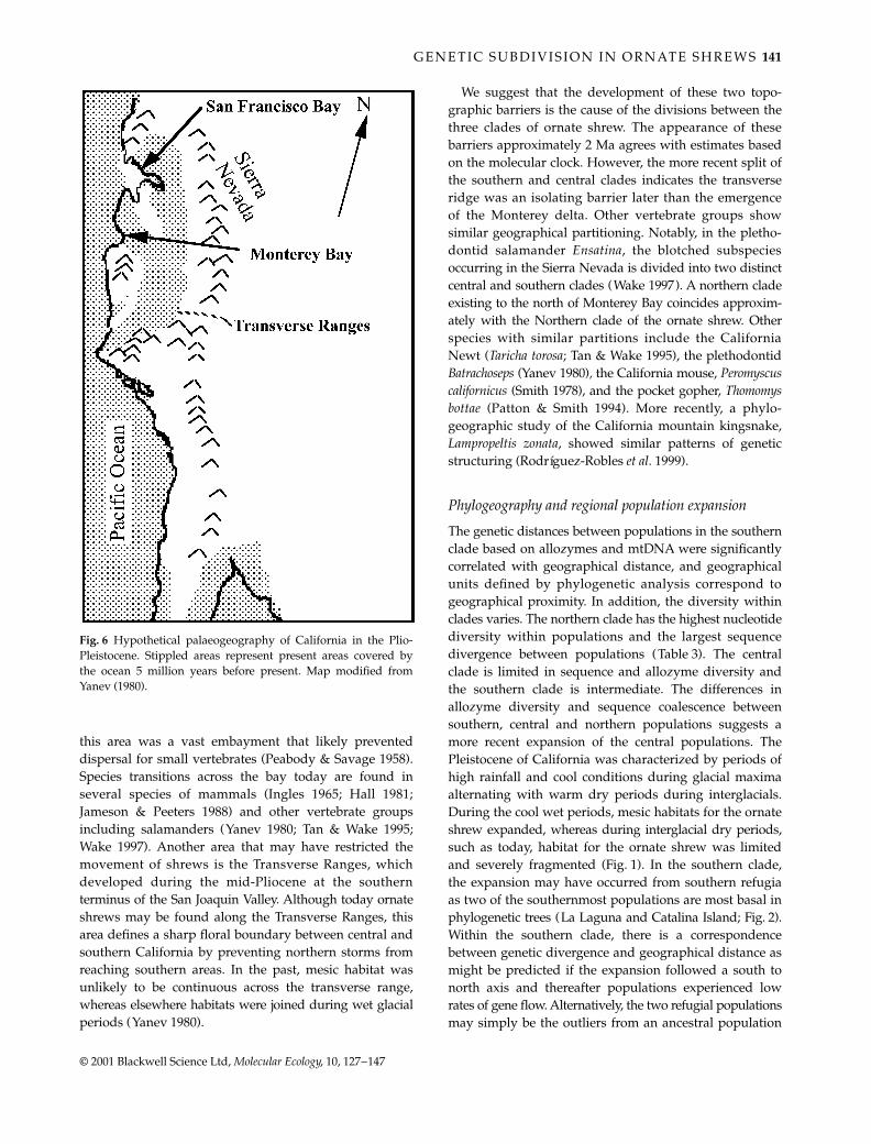
Approximately 5 Ma the orogeny of the Sierra Nevadaand Coast Ranges was initiated and large areas in centraland southern California were covered by sea (Wahrhaftig& Birman 1965). Throughout much of the period thatfollowed, the San Joaquin Valley was a wide seaway ratherthan the present-day continental river valley (Fig. 6). Mesichabitats suitable for shrews were restricted to the marginof this seaway. Two significant barriers to dispersal emergedacross the central valley during the Plio-Pleistocene (Fig. 6).The most profound barrier likely developed at the point
MEC1178.fm Page 139 Friday, December 8, 2000 3:38 PM
140 J . E . M A L D O N A D O , C . V I L À and R . K . WAY N E
© 2001 Blackwell Science Ltd, Molecular Ecology, 10, 127–147
where the present day Central Valley drains into thePacific Ocean near Monterey Bay. For various periodsduring the Pliocene, precursor drainages of the pre-sent-day Central Valley entered the Pacific Ocean in the
vicinity of the present-day Monterey Bay where the largestmarine canyon (of Grand Canyon scale) on the Pacificcoast of north America is found (Yanev 1980). Beginningapproximately 10 Ma and for most of the Plio-Pleistocene,
Fig. 5 Unrooted neighbour-joining tree based on the proportion of shared alleles between shrew allozyme genotypes. Shrews from northernpopulations are indicated with continuous lines, from central populations with dashed lines and from southern populations with dotted lines.
MEC1178.fm Page 140 Friday, December 8, 2000 3:38 PM
G E N E T I C S U B D I V I S I O N I N O R N AT E S H R E W S 141
© 2001 Blackwell Science Ltd, Molecular Ecology, 10, 127–147
this area was a vast embayment that likely preventeddispersal for small vertebrates (Peabody & Savage 1958).Species transitions across the bay today are found inseveral species of mammals (Ingles 1965; Hall 1981;Jameson & Peeters 1988) and other vertebrate groupsincluding salamanders (Yanev 1980; Tan & Wake 1995;Wake 1997). Another area that may have restricted themovement of shrews is the Transverse Ranges, whichdeveloped during the mid-Pliocene at the southernterminus of the San Joaquin Valley. Although today ornateshrews may be found along the Transverse Ranges, thisarea defines a sharp floral boundary between central andsouthern California by preventing northern storms fromreaching southern areas. In the past, mesic habitat wasunlikely to be continuous across the transverse range,whereas elsewhere habitats were joined during wet glacialperiods (Yanev 1980).
We suggest that the development of these two topo-graphic barriers is the cause of the divisions between thethree clades of ornate shrew. The appearance of thesebarriers approximately 2 Ma agrees with estimates basedon the molecular clock. However, the more recent split ofthe southern and central clades indicates the transverseridge was an isolating barrier later than the emergenceof the Monterey delta. Other vertebrate groups showsimilar geographical partitioning. Notably, in the pletho-dontid salamander Ensatina, the blotched subspeciesoccurring in the Sierra Nevada is divided into two distinctcentral and southern clades (Wake 1997). A northern cladeexisting to the north of Monterey Bay coincides approxim-ately with the Northern clade of the ornate shrew. Otherspecies with similar partitions include the CaliforniaNewt (Taricha torosa; Tan & Wake 1995), the plethodontidBatrachoseps (Yanev 1980), the California mouse, Peromyscuscalifornicus (Smith 1978), and the pocket gopher, Thomomysbottae (Patton & Smith 1994). More recently, a phylo-geographic study of the California mountain kingsnake,Lampropeltis zonata, showed similar patterns of geneticstructuring (Rodríguez-Robles et al. 1999).
Phylogeography and regional population expansion
The genetic distances between populations in the southernclade based on allozymes and mtDNA were significantlycorrelated with geographical distance, and geographicalunits defined by phylogenetic analysis correspond togeographical proximity. In addition, the diversity withinclades varies. The northern clade has the highest nucleotidediversity within populations and the largest sequencedivergence between populations (Table 3). The centralclade is limited in sequence and allozyme diversity andthe southern clade is intermediate. The differences inallozyme diversity and sequence coalescence betweensouthern, central and northern populations suggests amore recent expansion of the central populations. ThePleistocene of California was characterized by periods ofhigh rainfall and cool conditions during glacial maximaalternating with warm dry periods during interglacials.During the cool wet periods, mesic habitats for the ornateshrew expanded, whereas during interglacial dry periods,such as today, habitat for the ornate shrew was limitedand severely fragmented (Fig. 1). In the southern clade,the expansion may have occurred from southern refugiaas two of the southernmost populations are most basal inphylogenetic trees (La Laguna and Catalina Island; Fig. 2).Within the southern clade, there is a correspondencebetween genetic divergence and geographical distance asmight be predicted if the expansion followed a south tonorth axis and thereafter populations experienced lowrates of gene flow. Alternatively, the two refugial populationsmay simply be the outliers from an ancestral population
Fig. 6 Hypothetical palaeogeography of California in the Plio-Pleistocene. Stippled areas represent present areas covered bythe ocean 5 million years before present. Map modified fromYanev (1980).
MEC1178.fm Page 141 Friday, December 8, 2000 3:38 PM
142 J . E . M A L D O N A D O , C . V I L À and R . K . WAY N E
© 2001 Blackwell Science Ltd, Molecular Ecology, 10, 127–147
that was widespread in Baja and southern California. Asgeological processes changed the climate and movedCatalina Island to the north relative to the Cape region ofBaja California, they also isolated these populations. Themainland populations of southern and northern BajaCalifornia subsequently evolved and differentiated, as wefind them today.
Previous evolutionary hypotheses concerning the radi-ation of shrews in general (Findley 1955; Carraway 1990)have drawn on the conventional wisdom that Pleistoceneclimatic cycles precipitated a large portion of speciationevents between extant sister taxa. A typical Pleistocenespeciation scenario would suggest that a widespreadancestral population became isolated into separateglacial refugia where allopatric divergence leading tospeciation was initiated (Hewitt 1996). Recently, thisparadigm was challenged for avian species because 70% ofbird species had genetic distance suggesting divergenceover 5 Ma (Klicka & Zink 1997). However, many intra-specific divergences do date to Pleistocene events (Avise& Walker 1998) suggesting Ice Ages are important causesof differentiation. The tripartite division of ornate shrewpopulations dates to the early Pleistocene and does notreflect isolation in recent Ice Age refugia. In contrast, pastpatterns of genetic divergence within clades appear to beerased by population contractions during interglacialsand re-established during glacial period expansions. Infact, a similar pattern of highly divergent clades, eachwith a recent coalescence, was found in a survey of Euro-pean species (Taberlet et al. 1998). This suggests the IceAge effects may have more pronounced impact on regionalwithin clade diversity than on speciation.
The evolutionary origin of the ornate shrew
The northern clade is the most basal in mitochondrial andallozyme trees, suggesting that the northern populationsof ornate and vagrant shrews are ancestral. The oldestknown Pliocene Sorex from the Nearctic was found inthe early Blancan Fox Canyon (Kansas) and Hagermanfaunas (Idaho) approximately 3.5 Ma. The first fossilprecursor of Sorex vagrans, S. hoyi and S. fumeus appearsin the late Kansan (Cudahy fauna of Kansas) about700 000 years ago (Kurtén & Anderson 1980), much morerecently than suggested by the molecular data (1.3–1.6 Ma). However, the climatic conditions and borealfloral assemblage present in South-west during thePlio-Pleistocene were unfavourable to fossil deposition(Dietling 1968) and the fossil record of Sorex in NorthAmerica is scanty (Kurtén 1967; Repenning 1967; Kurtén& Anderson 1980; Lundelius et al. 1983; Carraway 1990).Thus, the fossil data may substantially underestimatedivergence time in shrews. In addition, palaeontologistshave not attempted to distinguish between S. monticolus
and S. vagrans when identifying fossil remains. Thus, it isnot unreasonable to suggests that ancestors of this groupof Sorex occurred within boreal floral assemblages presentin the western US before the Pleistocene (Dietling 1968;Carraway 1990). Our results suggest that much older fossilsof S. ornatus, S. vagrans and S. monticolus may be found.
Relationship of S. ornatus, S. vagrans and S. monticolus
S. monticolus, S. vagrans and S. ornatus are part of a groupof closely related taxa included in the subgenus Otisorex.Distinguishing between these taxa has been difficultwhere the ranges of species overlap (George & Smith1991). In the past, S. monticolus and S. vagrans have beenvariously identified as one or multiple species by differ-ent authors (e.g. Findley 1955; Brown 1974; Hennings& Hoffmann 1977; van Zyll de Jong 1982; George 1988;Carraway 1990). The results of our mtDNA analysissuggest that S. monticolus diverged from S. vagrans andS. ornatus approximately 1.6 Ma and should be con-sidered a different species. A problematic finding concernsthe inclusion of sequences from S. ornatus sinuosus andS. o. californicus in the northern clade that is otherwisecomposed of sequences from S. vagrans (Fig. 2), makingS. ornatus a paraphyletic group. Four conceivable causescould give rise to the clustering of S. vagrans and ornateshrew sequences. First, hybridization may have occurredbetween the two species in northern California wheretheir ranges meet. Mitochondrial haplotypes observed invagrant shrews could have originated, in fact, in ornateshrews, or vice versa. Past morphological studies of shrewsfrom the San Pablo Bay (in the San Francisco Bay area)showed that they were intermediate in external measure-ments and colour between S. v. vagrans and S. o. sinuosus(Rudd 1955a; Brown & Rudd 1981). However, northernpopulations do not show significant levels of gametic andcytonuclear disequilibrium that would be expected inhybridizing populations. Levels of disequilibrium are lessthan 1% of all pairwise comparisons between loci in all 22populations of ornate shrew. Thus, if hybridization occurredit must be ancient because no disequilibrium can bedetected. To further assess the possibility of hybridization,we sequenced a specimen of S. vagrans from the JarbridgeMountains near Elko Nevada and the border with Idaho,approximately 400 miles from the presumed contact zoneof the two species. S. vagrans has a distribution above2000 meters in the eastern Slope of the Sierra Nevadamountains (Hennings & Hoffmann 1977), ranging fromnorthern California to the northern Great basin and theColumbia Plateau (Fig. 1). In contrast, the ornate shrew isthought to be a lowland form restricted to California andBaja California (Owen & Hoffman 1983). S. ornatus is alsothe only shrew species occupying the blue oak/diggerpine forest at the lowest elevations of the western slope of
MEC1178.fm Page 142 Friday, December 8, 2000 3:38 PM
G E N E T I C S U B D I V I S I O N I N O R N AT E S H R E W S 143
© 2001 Blackwell Science Ltd, Molecular Ecology, 10, 127–147
the Sierra Nevada below 1200 m (Williams 1991). TheS. vagrans haplotype from Nevada was classified withinthe northern clade of ornate shrew sequences in Fig. 2and with the other haplotypes of S. vagrans. A hybridzone of this extent is unlikely for a species of such limitedmobility (Owen & Hoffmann 1983). Therefore, hybridiza-tion is an unlikely cause of the paraphyletic pattern.Additionally, all individuals with S. ornatus morphologyin northern California have cytochrome b sequencessimilar to S. vagrans.
A second explanation is that lineage sorting is incom-plete in ornate shrews such that long ancestral lineagesare retained in the northern populations (Avise 1989).However, the S. vagrans haplotypes in the northern cladeare not found in any other clades and are recently divergedfrom sequences in the northern clade. These findingscontradict the expectation of incomplete lineage sorting.
A third explanation is that S. vagrans and S. ornatus aresimply ecotypes of the same species. However, this is notconsistent with the large sequence divergence betweenclades. The mean sequence divergence between the com-plete 699 bp sequences in the northern clade and those inthe southern clade is 7.0% (4.2% between southern andcentral clades). In a phylogenetic study of cytochrome bsequences (1011 bp in length) across Sorex shrews though-out the world, Fumagalli et al. (1999) observed intraspecificdistances ranging from 0 to 5.2%. Only in one case didthey observe an instance of an exceptionally large diver-gence, up to 9.2%, in two well-differentiated subspecies ofS. arcticus. The large divergence that we observed separ-ating the northern clade from the central and southernclades suggest that they may correspond to different species.
Finally, populations in the northern clade may bemisclassified as ornate shrews. In fact, ornate shrews areremarkably uniform phenotypically and cannot be easilydistinguished from S. vagrans in northern California (Rudd1955b; Brown 1971; Junge & Hoffmann 1981). Consequently,we conclude that the northern ornate shrews may repres-ent a lowland form of vagrant shrews with a morphologyresembling the ornate shrews, not closely related to ornateshrews from south of San Francisco Bay. Presumably thenorthern California ornate shrews are derived from S. vagransthat have a high altitude distribution in the Sierra Nevadamountains, whereas the southern and central clade evolvedindependently from a southern California ancestor.
Units for conservation
The ornate shrew is one of the most threatened smallmammals in southern (Williams 1986) and Baja California(Elliot 1903; Huey 1964; Woloszyn et al. 1985; Maldonado1999). It is thought to be threatened primarily due todestruction of wetlands and riparian habitats, and foursubspecies (S. o. salicornicus, relictus, willetti and sinuosus)
are listed as California Mammal Species of Special Concern.In Baja California, our field surveys also revealed that thefew remaining populations are small and fragmented andhave a high probability of extinction (Maldonado 1999).Ornate shrews may once have had a continuous distributionalong the marshlands of Tulare Basin in the San JoaquinValley (Grinnell 1932), but this habitat is now greatly frag-mented due to cultivation and the recent disappearanceof lakes and sloughs. Similarly, the loss of habitat due todevelopment along the California coast may have causedthe extirpation of numerous ornate shrew populations(Williams 1986).
Our results suggest that the southern and central popu-lations of the ornate shrew form two distinct clades thathave long and separate ancestry. Therefore, each is anevolutionary significant unit because they are reciprocallymonophyletic and divergent in allele frequencies (Moritz1995). Therefore, they should be managed as separateunits for conservation. Moreover, within each region, geneflow is low among populations and nearly all have differ-ent mtDNA sequences and are differentiated with regardto allozyme allele frequencies (Tables 3–5). Therefore,these populations should be considered managementunits as they will respond independently to environmentalchanges (Moritz 1995). Once populations disappear theyare unlikely to be recolonized from elsewhere. In addition,populations on Santa Catalina Island and the relictualpopulation in Baja California are genetically the mostdistinct populations in the southern clade and are alsothe most endangered. Special attention needs to be placedon their conservation. Collaborative efforts between U.S.and Mexican federal governmental agencies are urgentlyneeded to preserve coastal marshes, wetlands, andriparian habitats and to protect the few remaining popu-lations of ornate shrews in southern and Baja California.
Finally, the populations north of San Francisco Bay maydefine a group having an independent origination fromS. vagrans ancestors. Therefore, the conservation status ofthe northern populations may need to be re-evaluated inlight of these newly discovered systematic affinities. Inparticular, efforts should be concentrated on elucidatingthe phylogenetic relationships of the threatened SaltMarsh Wandering shrew (S. v. halicoetes) which inhabitsthe salt marsh ecosystem of the San Francisco Bay areaand is distinguished from other shrews in the area basedon dubious phenotypic characteristics (i.e. dark pelagecolouration and distribution). S. o. sinuosus was also ori-ginally considered a separate species because it wasendemic to tide marshes and had a melanistic pelage(Rudd 1955b), but our results show this taxon is notdifferentiated from other northern populations. Pastmorphological studies of shrews from this area havebeen problematic and controversial (Rudd 1955a; Brown &Rudd 1981). The problems with the systematics of this
MEC1178.fm Page 143 Friday, December 8, 2000 3:38 PM
144 J . E . M A L D O N A D O , C . V I L À and R . K . WAY N E
© 2001 Blackwell Science Ltd, Molecular Ecology, 10, 127–147
group of shrews have led Ingles (1965) and Hall (1981) tosuggest that a future reviser might arrange both sinuosusand ornatus as subspecies of S. vagrans. Our resultssuggest that northern populations of the ornate shrew maybe a unique lowland form of the vagrant shrew that hasconverged independently on the morphology of southernand central California S. ornatus.
Acknowledgements
We thank K. Stager, F. Hertel, for assistance in the field andencouragement and support throughout the project. S. B. Georgehelped and advised in the processing and analysis of the allozymeportion of this study. J. Leonard and K. Sainz assisted in laboratoryprocedures. L. Simons, R. Fisher, R. Matoni, D. Holland, D. Janniger,H. Stager donated specimens. D. Jacobs gave insightful commentson the palaeogeography of California. D. Buth, C. Marshall,L. Shapiro K. Omland and M. Gompper provided a carefulcritique that greatly improved this manuscript. We thank theCalifornia Nature Conservancy, Catalina Island Conservancy,USFWS and California Department of Fish and Game for grant-ing permits and allowing access to State and Federal wildlifereserves throughout California and SEDUE for granting permitsto work in Mexico. This work was supported by funding fromASM grants in aid of research, Sigma Xi, the Theodore RooseveltMemorial Fund, and The Section of Mammals of the Los AngelesCounty Museum of Natural History.
References
Avise JC (1989) Gene trees and organismal histories: a phylo-genetic approach to population biology. Evolution, 43, 1192–1208.
Avise JC (1992) Molecular population structure and the biogeo-graphic history of a regional fauna: a case history with lessonsfor conservation biology. Oikos, 63, 62–76.
Avise JC, Walker D (1998) Pleistocene phylogeographic effects onavian populations and the speciation process. Proceedings of theRoyal Society of London Series B, 265, 457–463.
Baker RJ, Taddei VA, Hudgeons JL et al. (1994) Systematic relation-ships within Chiroderma (Chiroptera: Phyllostomatidae) basedon cytochrome b sequence variation. Journal of Mammalogy, 75,321–327.
Brown RJ (1971) A comparative study of the chromosomes of somePacific coast shrews (Genus Sorex). PhD Dissertation. Universityof California, Davis.
Brown RJ (1974) A comparative study of the chromosomes ofthree species of shrews, Sorex bendirii, Sorex trowbridgii, andSorex vagrans. Wasmann Journal of Biology, 32, 303–326.
Brown RJ, Rudd RL (1981) Chromosomal comparisons within theSorex ornatus–S. vagrans complex. Wasmann Journal of Biology,39, 30–35.
Carraway LN (1990) A morphologic and morphometric analysisof the ‘Sorex vagrans species complex’ in the Pacific Coast region.Special Publications of the Museum of Texas Tech University, 32,1–78.
Collins PW, George SB (1990) Systematics and taxonomy ofisland and mainland populations of Reithrodontomys megalotisin southern California. Contributions in Science, Natural HistoryMuseum of Los Angeles County, 420, 1–26.
Dietling LE (1968) Historical background of the flora of the PacificNorthwest. Bulletin of the Museum of Natural History, Universityof Oregon, 13, 1–57.
Elliot DG (1903) A List of a Collection of Mexican Mammals withDescriptions of Some Apparently New Forms. Field ColumbianMuseum Publications. 71, Zoology Series, 3, 141–149.
Excoffier L, Smouse PE, Quatro JM (1992) Analysis of molecularvariance inferred from metric distance among DNA haplotypes:application to human mitochondrial DNA restriction data.Genetics, 131, 479–491.
Farris JS (1970) Methods of computing Wagner trees. SystematicZoology, 19, 83–92.
Felsenstein J (1985) Confidence limits on phylogenies: an approachusing the bootstrap. Evolution, 39, 783–791.
Felsenstein J (1989) PHYLIP-Phylogenetic Inference Package, Version 3.2.University of Washington, Seattle Washington.
Findley JS (1955) Speciation of the wandering shrew. Universityof Kansas Publications, Museum of Natural History, 9, 1–68.
Fumagalli L, Taberlet P, Stewart DT, Gielly L, Hausser J, Vogel P(1999) Molecular phylogeny and evolution of Sorex shrews(Soricidae: Insectivora) inferred from mitochondrial DNAsequence data. Molecular Phylogenetics and Evolution, 11, 222–235.
George SB (1988) Systematics, historical biogeography, andevolution of the genus Sorex. Journal of Mammalogy, 69, 443–461.
George SB, Smith JD (1991) Inter- and intra-specific variabilityamong coastal and island populations of Sorex monticolus andSorex vagrans in the Pacific Northwest. Special Publications,Museum of Southwestern Biology, University of New Mexico, 1,75–91.
Girman DJ (1996) The use of PCR-based single-stranded con-formation polymorphism analysis (PCR–SSCP) in conservationgenetics. In: Molecular Genetic Approaches in Conservation (edsSmith T, Wayne RK), pp. 167–182 Oxford University Press,New York.
Green PM, Bentley DR, Mibashan RS, Nilson IM, Gianelli F(1989) Molecular pathology of haemophilia B. EuropeanMolecular Biology Organization Journal, 8, 1067–1072.
Grinnell J (1932) A relic shrew from central California. Universityof California Publications in Zoology, 38, 389–390.
Hall ER (1981) The mammals of North America. John Wiley andSons, New York.
Hartl DL, Clark AG (1990) Principles of Population Genetics. 2ndedn. Sinauer Associates, Sunderland, Massachusetts.
Hennings D, Hoffmann RS (1977) A review of the taxonomy ofthe Sorex vagrans species complex from western North America.Occasional Papers of the Museum of Natural History, University ofKansas, 68, 1–35.
Hewitt GM (1996) Some genetic consequences of ice ages, andtheir role in divergence and speciation. Biological Journal of theLinnean Society, 58, 247–276.
Higgins DG, Sharp PM (1989) Fast and sensitive multiple sequencealignment on a microcomputer. Cabios, 5, 151–153.
Hill WG, Robertson A (1968) Linkage disequilibrium in finitepopulations. Theoretical Applied Genetics, 38, 226–231.
Hillis DM, Mable BK, Moritz C (1996) Applications of molecularsystematics: The state of the field and a look to the future.In: Molecular Systematics (eds Hillis DM, Moritz C, Mable BK),pp. 515–543. Sinauer, Sunderland, Massachusetts.
Huey LM (1964) The mammals of Baja California, Mexico. Trans-actions of the San Diego Society of Natural History, 13, 85–168.
Ingles LG (1965) Mammals of the Pacific States. Stanford UniversityPress, Stanford, California.
MEC1178.fm Page 144 Friday, December 8, 2000 3:38 PM
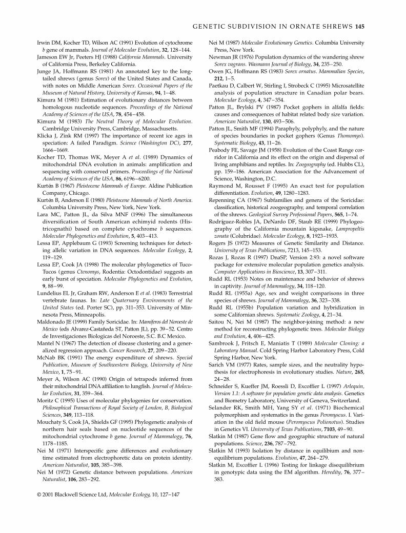
G E N E T I C S U B D I V I S I O N I N O R N AT E S H R E W S 145
© 2001 Blackwell Science Ltd, Molecular Ecology, 10, 127–147
Irwin DM, Kocher TD, Wilson AC (1991) Evolution of cytochromeb gene of mammals. Journal of Molecular Evolution, 32, 128–144.
Jameson EW Jr, Peeters HJ (1988) California Mammals. Universityof California Press, Berkeley California.
Junge JA, Hoffmann RS (1981) An annotated key to the long-tailed shrews (genus Sorex) of the United States and Canada,with notes on Middle American Sorex. Occasional Papers of theMuseum of Natural History, University of Kansas, 94, 1–48.
Kimura M (1981) Estimation of evolutionary distances betweenhomologous nucleotide sequences. Proceedings of the NationalAcademy of Sciences of the USA, 78, 454–458.
Kimura M (1983) The Neutral Theory of Molecular Evolution.Cambridge University Press, Cambridge, Massachusetts.
Klicka J, Zink RM (1997) The importance of recent ice ages inspeciation: A failed Paradigm. Science (Washington DC), 277,1666–1669.
Kocher TD, Thomas WK, Meyer A et al. (1989) Dynamics ofmitochondrial DNA evolution in animals: amplification andsequencing with conserved primers. Proceedings of the NationalAcademy of Sciences of the USA, 86, 6196–6200.
Kurtén B (1967) Pleistocene Mammals of Europe. Aldine PublicationCompany, Chicago.
Kurtén B, Anderson E (1980) Pleistocene Mammals of North America.Columbia University Press, New York, New York.
Lara MC, Patton JL, da Silva MNF (1996) The simultaneousdiversification of South American echimyid rodents (His-tricognathi) based on complete cytochrome b sequences.Molecular Phylogenetics and Evolution, 5, 403–413.
Lessa EP, Applebaum G (1993) Screening techniques for detect-ing allelic variation in DNA sequences. Molecular Ecology, 2,119–129.
Lessa EP, Cook JA (1998) The molecular phylogenetics of Tuco-Tucos (genus Ctenomys, Rodentia: Octodontidae) suggests anearly burst of speciation. Molecular Phylogenetics and Evolution,9, 88–99.
Lundelius EL Jr, Graham RW, Anderson E et al. (1983) Terrestrialvertebrate faunas. In: Late Quaternary Environments of theUnited States (ed. Porter SC), pp. 311–353. University of Min-nesota Press, Minneapolis.
Maldonado JE (1999) Family Soricidae. In: Mamiferos del Noroeste deMexico (eds Alvarez-Castañeda ST, Patton JL), pp. 39–52. Centrode Investigaciones Biologicas del Noroeste, S.C. B.C Mexico.
Mantel N (1967) The detection of disease clustering and a gener-alized regression approach. Cancer Research, 27, 209–220.
McNab BK (1991) The energy expenditure of shrews. SpecialPublication, Museum of Southwestern Biology, University of NewMexico, 1, 75–91.
Meyer A, Wilson AC (1990) Origin of tetrapods inferred fromtheir mitochondrial DNA affiliation to lungfish. Journal of Molecu-lar Evolution, 31, 359–364.
Moritz C (1995) Uses of molecular phylogenies for conservation.Philosophical Transactions of Royal Society of London, B, BiologicalSciences, 349, 113–118.
Mouchaty S, Cook JA, Shields GF (1995) Phylogenetic analysis ofnorthern hair seals based on nucleotide sequences of themitochondrial cytochrome b gene. Journal of Mammalogy, 76,1178–1185.
Nei M (1971) Interspecific gene differences and evolutionarytime estimated from electrophoretic data on protein identity.American Naturalist, 105, 385–398.
Nei M (1972) Genetic distance between populations. AmericanNaturalist, 106, 283–292.
Nei M (1987) Molecular Evolutionary Genetics. Columbia UniversityPress, New York.
Newman JR (1976) Population dynamics of the wandering shrewSorex vagrans. Wasmann Journal of Biology, 34, 235–250.
Owen JG, Hoffmann RS (1983) Sorex ornatus. Mammalian Species,212, 1–5.
Paetkau D, Calbert W, Stirling I, Strobeck C (1995) Microsatelliteanalysis of population structure in Canadian polar bears.Molecular Ecology, 4, 347–354.
Patton JL, Brylski PV (1987) Pocket gophers in alfalfa fields:causes and consequences of habitat related body size variation.American Naturalist, 130, 493–506.
Patton JL, Smith MF (1994) Paraphyly, polyphyly, and the natureof species boundaries in pocket gophers (Genus Thomomys).Systematic Biology, 43, 11–26.
Peabody FE, Savage JM (1958) Evolution of the Coast Range cor-ridor in California and its effect on the origin and dispersal ofliving amphibians and reptiles. In: Zoogeography (ed. Hubbs CL),pp. 159–186. American Association for the Advancement ofScience, Washington, D.C.
Raymond M, Rousset F (1995) An exact test for populationdifferentiation. Evolution, 49, 1280–1283.
Repenning CA (1967) Subfamilies and genera of the Soricidae:classification, historical zoogeography, and temporal correlationof the shrews. Geological Survey Professional Papers, 565, 1–74.
Rodríguez-Robles JA, DeNardo DF, Staub RE (1999) Phylogeo-graphy of the California mountain kigsnake, Lampropeltiszonata (Colubridae). Molecular Ecology, 8, 1923–1935.
Rogers JS (1972) Measures of Genetic Similarity and Distance.University of Texas Publications, 7213, 145–153.
Rozas J, Rozas R (1997) DnaSP, Version 2.93: a novel softwarepackage for extensive molecular population genetics analysis.Computer Applications in Bioscience, 13, 307–311.
Rudd RL (1953) Notes on maintenance and behavior of shrewsin captivity. Journal of Mammalogy, 34, 118–120.
Rudd RL (1955a) Age, sex and weight comparisons in threespecies of shrews. Journal of Mammalogy, 36, 323–338.
Rudd RL (1955b) Population variation and hybridization insome Californian shrews. Systematic Zoology, 4, 21–34.
Saitou N, Nei M (1987) The neighbor-joining method: a newmethod for reconstructing phylogenetic trees. Molecular Biologyand Evolution, 4, 406–425.
Sambrook J, Fritsch E, Maniatis T (1989) Molecular Cloning: aLaboratory Manual. Cold Spring Harbor Laboratory Press, ColdSpring Harbor, New York.
Sarich VM (1977) Rates, sample sizes, and the neutrality hypo-thesis for electrophoresis in evolutionary studies. Nature, 265,24–28.
Schneider S, Kueffer JM, Roessli D, Excoffier L (1997) Arlequin,Version 1.1: A software for population genetic data analysis. Geneticsand Biometry Laboratory, University of Geneva, Switzerland.
Selander RK, Smith MH, Yang SY et al. (1971) Biochemicalpolymorphism and systematics in the genus Peromyscus. I. Vari-ation in the old field mouse (Peromyscus Polionotus). Studiesin Genetics VI. University of Texas Publications, 7103, 49–90.
Slatkin M (1987) Gene flow and geographic structure of naturalpopulations. Science, 236, 787–792.
Slatkin M (1993) Isolation by distance in equilibium and non-equilibrium populations. Evolution, 47, 264–279.
Slatkin M, Excoffier L (1996) Testing for linkage disequilibriumin genotypic data using the EM algorithm. Heredity, 76, 377–383.
MEC1178.fm Page 145 Friday, December 8, 2000 3:38 PM
146 J . E . M A L D O N A D O , C . V I L À and R . K . WAY N E
© 2001 Blackwell Science Ltd, Molecular Ecology, 10, 127–147
Smith MF (1978) Geographic variation in genic and morpholo-gical characters in Peromyscus californicus. Journal of Mammalogy,60, 705–722.
Smith MF, Patton JL (1993) The diversification of South Americanmurid rodents: Evidence from mitochondrial DNA sequencedata for the akodontine tribe. Biological Journal of the LinneanSociety, 50, 149–177.
Stanley HF, Casey S, Carnahan JM, Goodman S, Harwood J,Wayne RK (1996) Worldwide patterns of mitochondrial DNAdifferentiation in the harbor seal (Phoca vitulina). MolecularBiology and Evolution, 13, 368–382.
Swofford DL (1993) Phylogenetic Analysis Using Parsimony (PAUP),Version 3.1.1. Illinois Natural History Survey, Champaign, Illinois.
Swofford DL, Selander RB (1981) biosys-1: a fortran program forthe comprehensive analysis of electrophoretic data in popula-tion genetics and systematics. Journal of Heredity, 72, 281–283.
Taberlet PL, Fumagalli L, Wust-Saucy AG, Cousson JF (1998)Comparative phylogeography and post glacial colonizationroutes in Europe. Molecular Ecology, 7, 453–464.
Tajima F (1989) Statistical method for testing the neutral mutationhypothesis by DNA polymorphism. Genetics, 123, 585–595.
Tan A-M, Wake DB (1995) mtDNA phylogeography of theCalifornia Newt, Taricha torosa (Caudata, Salamandridae).Molecular Phylogenetics and Evolution, 4, 383–394.
Tolliver DK, Smith MH, Leftwich RH (1985) Genetic variabilityin Insectivora. Journal of Mammalogy, 66, 405–410.
Wahrhaftig C, Birman JH (1965) The Quaternary of the Pacificmountain system in California. In: The Quaternary of the UnitedStates (eds Wright HE Jr, Frey DG), pp. 299–331. PrincetonUniversity Press, Princeton, New Jersey.
Wake DB (1997) Incipient species formation in salamanders ofthe Ensatina complex. Proceedings of the National Academy ofSciences of the USA, 94, 7761–7767.
Waser PM, Strobeck C (1998) Genetic signatures of interpopula-tion dispersal. TREE, 13, 43–44.
Williams DF (1986) Mammalian species of special concern inCalifornia. Wildlife Management Division Administrative Report86–1 ( June, 1986).
Williams DF (1991) Habitats of shrews (Genus Sorex) in forestcommunities of the western Sierra Nevada, California. SpecialPublications, Museum of Southwestern Biology, University of NewMexico, 1, 1–14.
Wilson AC, Cann RL, Carr SM et al. (1985) Mitochondrial DNAand two perspectives on evolutionary genetics. Biological Journalof the Linnean Society, 26, 375–400.
Winship PR (1989) An improved method for directly sequencingPCR amplified material using DMSO. Nucleic Acid Research, 17,1266.
Woloszyn D, Guemez JC, Woloszyn BW (1985) New LocalityRecord of La Laguna Mountain Shrew, Sorex ornatus lagunaeNelson et Goldman, 1909, in Cape Region of Baja California,Mexico. Acta Theriologica, 30, 157–167.
Wright S (1969) Evolution and the Genetics of Populations. 2. TheTheory of Gene Frequencies. University of Chicago Press, Chicago,Illinois.
Wright S (1978) Evolution and the Genetics of Populations. 4.Variability Within and Among Natural Populations. University ofChicago Press, Chicago, Illinois.
Wright JW (1983) The evolution and biogeography of the lizardsof the Galapagos Archipielago: Evolutionary genetics ofPhyllodactylus and Tropidurus populations. In: Patterns ofEvolution in Galapagos Organisms (eds Bowman RI, Berson M,Levition A), pp. 123–155. American Association for theAdvancement of Science, Pacific Division, San Francisco.
Yanev KP (1980) Biogeography and distribution of three parapatricsalamander species in coastal and borderland California. In: TheCalifornia Islands: Proceedings of a Multidisciplinary Symposium(ed. Power DM), pp. 531–549, Santa Barbara Museum of NaturalHistory, Santa Barbara, California.
van Zyll de Jong CG (1982) An additional morphological characteruseful in distinguishing two similar shrews, Sorex monticolusand Sorex vagrans. Canadian Field Naturalist, 96, 349–350.
This study is part of the PhD research of Jesús Maldonado,who was directed by Dr Robert K. Wayne. Jesús Maldonado isinterested in a variety of questions in evolutionary biology thatcan be answered with molecular tools. His primary interests arethe evolutionary genetics and conservation biology of mammals.Carles Vilà works on the population and conservation geneticsof mammals. Most of the laboratory analyses and all the dataanalyses were done in the Conservation Genetics laboratory ofDr Robert K. Wayne at UCLA.
MEC1178.fm Page 146 Friday, December 8, 2000 3:38 PM
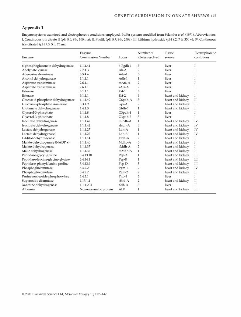
G E N E T I C S U B D I V I S I O N I N O R N AT E S H R E W S 147
© 2001 Blackwell Science Ltd, Molecular Ecology, 10, 127–147
Appendix 1
Enzyme systems examined and electrophoretic conditions employed. Buffer systems modified from Selander et al. (1971). Abbreviations:I, Continuous tris citrate II (pH 8.0; 8 h, 100 ma); II, Poulik (pH 8.7; 6 h, 250v); III, Lithium hydroxide (pH 8.2; 7 h, 350 v); IV, Continuoustris-citrate I (pH 7.5; 5 h, 75 ma)
EnzymeEnzyme Commission Number Locus
Number of alleles resolved
Tissue source
Electrophoretic conditions
6-phosphogluconate dehydrogenase 1.1.1.44 6-Pgdh-1 3 liver IAdelynate kynase 2.7.4.3 Ak-A 2 liver IAdenosine deaminase 3.5.4.4 Ada-1 3 liver IAlcohol dehydrogenase 1.1.1.1 Adh-1 1 liver IAspartate transaminase 2.6.1.1 mAta-A 2 liver IAspartate transaminase 2.6.1.1 sAta-A 2 liver IEsterase 3.1.1.1 Est-1 3 liver IEsterase 3.1.1.1 Est-2 4 heart and kidney IGlucose-6-phosphate dehydrogenase 1.1.1.49 G6pdh-A 3 heart and kidney IIGlucose-6-phosphate isomerase 5.3.1.9 Gpi-A 2 heart and kidney IIIGlutamate dehydrogenase 1.4.1.3 Gtdh-1 1 heart and kidney IIGlycerol-3-phosphate 1.1.1.8 G3pdh-1 1 liver IGlycerol-3-phosphate 1.1.1.8 G3pdh-2 3 liver IIsocitrate dehydrogenase 1.1.1.42 mIcdh-A 1 heart and kidney IVIsocitrate dehydrogenase 1.1.1.42 sIcdh-A 3 heart and kidney IVLactate dehydrogenase 1.1.1.27 Ldh-A 1 heart and kidney IVLactate dehydrogenase 1.1.1.27 Ldh-B 1 heart and kidney IVL-Iditol dehydrogenase 1.1.1.14 Iddh-A 2 heart and kidney IMalate dehydrogenase (NADP +) 1.1.1.40 Mdhp-A 3 heart and kidney IMalate dehydrogenase 1.1.1.37 sMdh-A 2 heart and kidney IMalic dehydrogenase 1.1.1.37 mMdh-A 1 heart and kidney IPeptidase-glycyl-glycine 3.4.13.18 Pep-A 1 heart and kidney IIIPeptidase-leucine-glycine-glycine 3.4.14.1 Pep-B 1 heart and kidney IIIPeptidase-phenylalanine-proline 3.4.13.9 Pep-D 3 heart and kidney IIIPhosphoglucomutase 5.4.2.2 Pgm-1 2 heart and kidney IVPhosphoglucomutase 5.4.2.2 Pgm-2 2 heart and kidney IIPurine nucleoside phosphorylase 2.4.2.1 Pnp-1 5 liver ISuperoxide dismutase 1.15.1.1 sSod-A 2 heart and kidney IIXanthine dehydrogenase 1.1.1.204 Xdh-A 3 liver IIAlbumin Non-enzymatic protein ALB 1 heart and kidney III
MEC1178.fm Page 147 Friday, December 8, 2000 3:38 PM