Embed Size (px)
Citation preview
ISS
N 0
249-
6399
ISR
N IN
RIA
/RR
--47
81--
FR
+E
NG
ap por t de r ech er ch e
THÈME 1
INSTITUT NATIONAL DE RECHERCHE EN INFORMATIQUE ET EN AUTOMATIQUE
Blind Channel Estimation for DS-CDMA
Xenofon G. Doukopoulos and George V. Moustakides
N° 4781
March 2003

Unité de recherche INRIA RennesIRISA, Campus universitaire de Beaulieu, 35042 Rennes Cedex (France)
Téléphone : +33 2 99 84 71 00 — Télécopie : +33 2 99 84 71 71
Blind Channel Estimation for DS-CDMA
Xenofon G. Doukopoulos and George V. Moustakides
Thème 1 — Réseaux et systèmes
Rapport de recherche n° 4781 — March 2003 — 20 pages
Abstract: The problem of channel estimation in code-division multiple-access systemsis considered. Using only the spreading code of the user of interest, a technique is pro-posed to identify the impulse response of the multipath channel from the received datasequence. While existing blind methods suffer from high computational complexity (due tolarge SVDs) and sensitivity to accurate knowledge of the noise subspace rank, the proposedmethod overcomes both problems. By employing a computationally simple matrix powerthat requires no a-priori knowledge of the noise subspace rank, we obtain efficient estimatesof the noise subspace. The impulse response is then directly identified through a small sized(order of the channel) SVD or a least squares optimization. Both approaches (SVD and leastsquares) are also extended to accommodate for synchronization with respect to the user ofinterest. Extensive simulations demonstrate robustness of the proposed scheme and perfor-mance comparable to existing SVD techniques but at a lower computational cost.
Key-words: Channel estimation, CDMA.
Estimation Aveugle de Canal pour le DS-CDMA
Résumé : Nous traitons le problème de l’estimation de canal pour le système CDMA (CodeDivision Multiple Access). En utilisant uniquement la signature de l’utilisateur d’intérêt,nous proposons une technique pour identifier la réponse impulsionelle d’un canal à trajetsmultiples à partir de la séquence des données reçues. Alors que les méthodes aveuglesexistantes sont d’une grande complexité (à cause des grandes SVD) et nécessitent uneconnaissance exacte du rang du sous-espace bruit, la méthode proposée surmonte ces deuxproblèmes. Nous employons une puissanse de matrice simple à calculer qui n’exige aucuneconnaissance a-priori du rang du sous-espace bruit et on obtient des estimations efficaces dusous-espace bruit. La réponse impulsionelle est alors directement identifiée par une SVDde petit taille (de l’ordre du canal) ou bien par un problème aux moindres carrés. Les deuxtechniques sont également généralisées pour soutenir une synchronization avec l’utilisateurd’intérêt. Des simulations multiples démontrent la robustesse de la méthode proposée etune performance comparable aux techniques SVD qui existent déjà, mais avec un coût decalcul moindre.
Mots-clés : estimation de canal, CDMA.

Blind Channel Estimation for DS-CDMA i
Contents
1 Introduction. 1
2 Signal Model. 2
3 The Power Method. 4
4 Key Results. 64.1 Identifiability. . . . . . . . . . . . . . . . . . . . . . . . . . . . . . . . . . 74.2 Two Optimization Problems. . . . . . . . . . . . . . . . . . . . . . . . . . 9
5 Channel Estimation Method and Synchronization. 115.1 Synchronization. . . . . . . . . . . . . . . . . . . . . . . . . . . . . . . . 12
6 Simulations - Discussion. 156.1 Spreading Codes of Length 16. . . . . . . . . . . . . . . . . . . . . . . . . 156.2 Spreading Codes of Length 128. . . . . . . . . . . . . . . . . . . . . . . . 17
7 Conclusion. 19
RR n° 4781

Blind Channel Estimation for DS-CDMA 1
1 Introduction.
Code-division multiple-access (CDMA) implemented with direct-sequence (DS) spreadspectrum constitutes one of the most important emerging technologies in wireless commu-nications. It is well known that CDMA has been selected as the base for the 3-rd generationmobile telephone systems.
In a CDMA system users are capable of simultaneously transmitting in time, while oc-cupying the same frequency band, by using a unique signature waveform assigned to eachone of them. However, this important advantage does not come for free since it consti-tutes, at the same time, the main source of performance degradation. Indeed for every user,all other users play the role of (multiuser) interference. Several multiuser detectors havealready been proposed in the literature and extensively analyzed (for details see [7]). Allsuch detectors, in order to be practically implementable, require at least knowledge of thesignature waveform of the user of interest. Assuming availability of this information, is infact quite reasonable.
At the receiver end (the mobile unit), whenever CDMA signals propagate through amultipath environment, the effective signature signals are no longer the signature wave-forms but rather the convolution of these signals with the channel impulse response. Thiscombined waveform is also known as composite signature. Clearly, if we like to apply thedetection structures of [7] introduced for the non-dispersive channel we need to know (orefficiently estimate) the channel impulse response. Furthermore, it is only natural to expressa strong interest towards blind estimation methods, since this class of techniques does notrequire transmission of any training sequences.
Blind channel estimation methods for CDMA are considered in [8] and [4]. Both articlespropose the recovery of the channel impulse response through a two-step procedure. Thefirst step involves a large SVD in order to obtain a base for the noise subspace of the receivedsignal, and the second consists in applying either a small SVD [8] or a QR-decomposition[4] of the size of the channel in order to obtain the final impulse response estimate. Theemployment of large SVDs (i.e. first step) in real time applications, essentially limits theuse of these methods to small spreading codes. We should also mention that both approachesare very sensitive to the correct knowledge of the noise subspace rank. This parameter isnot constant since it changes with the number of users accessing the CDMA channel. Itturns out that even the slightest erroneous rank estimate can lead to drastic performancedegradation.
An alternative approach is proposed in [6], where blind receivers are obtained through amax/min constrained optimization. Using the theoretical developments of this work, LMSand RLS blind adaptations are introduced in [9]. An extension of this work, using higherorder cumulants, is reported in [10]. However, the corresponding implementation suffers
RR n° 4781
2 Doukopoulos and Moustakides
from slow convergence even in the short code case while its success relies on the Gaussiannoise assumption, and in particular the fact that higher order cumulants of Gaussian randomvariables are zero.
The idea we propose in this work overcomes all drawbacks reported above for the al-ready existing schemes. Although our method follows the main lines of [8, 4], (involvingtwo steps) it is characterized by an essential difference. We replace the first large SVD stepby the computation of a matrix power. Despite the fact that, in theory, the power methodattains the performance of SVD only in the limit (as the power tends to infinity), in practicewe do not need to go beyond the third power. Furthermore this approach does not requireknowledge of the noise subspace rank thus its robustness, with respect to this parameter,is guaranteed. For the second step, we may proceed either with a small sized SVD [8], ora QR decomposition [4], or finally a simple least squares (LS) approach (proposed here).As far as the latter approach is concerned, it should be mentioned that it also lends itselfto the development of an efficient scheme for resolving the timing synchronization prob-lem. Extensive simulations demonstrate rapid convergence of our method and performancewhich is comparable to [8, 4] but with a significantly lower computational cost. As far asthe method of [6] is concerned, we should mention that the coincides with a special caseour SVD version. However in [6] no convincing explanation is provided as to why thisidea might be successful. We believe that with the setup introduced here this will becomesufficiently clear and, furthermore, with our extended version we will be able to obtainsignificant performance gains.
The rest of the paper is organized as follows. In Section II, we introduce a generalsignal model for the multipath CDMA system. In Section III we present a version of thepower method suitable for the channel estimation problem which is analyzed in SectionIV. The realistic case scenario and synchronization issues are treated in Section V. SectionVI contains a number of simulation comparisons between the proposed and the existingmethods, and finally Section VII concludes our article.
2 Signal Model.
Consider a K-user DS-CDMA system with identical chip waveforms and signaling antipo-dally through a multipath channel in the presence of additive white noise (AWN), not neces-sarily Gaussian. Although CDMA systems are continuous in time, they can be adequatelymodeled by an equivalent discrete time system [7]. Specifically, no information is lost if welimit ourselves to the output of a chip matched filter applied to the received analog signaland sampled at the chip rate [7].
INRIA
Blind Channel Estimation for DS-CDMA 3
Let N be the processing gain of the code and L the length of the channel impulse re-sponse. Let si = [si(0)si(1) · · · si(N−1)]t be the length N normalized signature waveform ofUser-i (i.e. ‖si‖ = 1), and denote by si(n) the infinite sequence generated by zero paddingthe signature si from both ends towards infinity. The transmitted signal due to User-i isgiven by
zi(n) = ai
∞
∑k=−∞
si(n− kN− τi)bi(k), i = 1, . . . ,K, (1)
where ai is the amplitude of User-i; bi(n) the corresponding bit sequence; and τi its initialdelay that can take any value in the set {0, . . . ,N − 1}. When zi(n) propagates through amultipath AWN channel with impulse response fi = [ fi(0) · · · fi(L−1)]t , then the receivedsignal y(n) can be written as
y(n) =K
∑i=1
zi(n)? fi(n)+σw(n)
=K
∑i=1
∞
∑k=−∞
ai si(n− kN− τi)bi(k)+σw(n), (2)
where ? denotes convolution; si(n) = si(n)? fi(n) is the convolution between the sequencesi(n) and the channel impulse response fi (i.e. the composite signature of User-i zero-paddedfrom both ends); and w(n) is a unit variance i.i.d. noise sequence with σ2 denoting the powerof the AWN.
Even though the model given in (2) fully describes the uplink (mobile to base station)scenario of a multipath CDMA system, it can be used for the downlink case (base stationto mobile) as well. Indeed in downlink, users are completely synchronized, therefore τ1 =· · ·= τK = τ, and they propagate through the same multipath channel, thus f1 = · · ·= fK = f.It is the latter case we are going to consider here, we should however note that, with almostno modifications, our methodology can be applied for the uplink case as well, in order toestimate the different channels one-by-one.
Without loss of generality, throughout this article, we will assume that the user of in-terest is User-1. At this point we will also assume that the initial delay τ is known andtherefore we have exact synchronization with the user of interest. This assumption is notrestrictive since it will be relaxed in Section V. For the presentation of our method it is moreconvenient to express the received signal in blocks of data. In particular we are interested inblocks of size mN + L− 1, where m is a positive integer. Consequently let us consider theblock
rm(n) = [y(nN) · · ·y((n−m)N−L+2)]t (3)
RR n° 4781
4 Doukopoulos and Moustakides
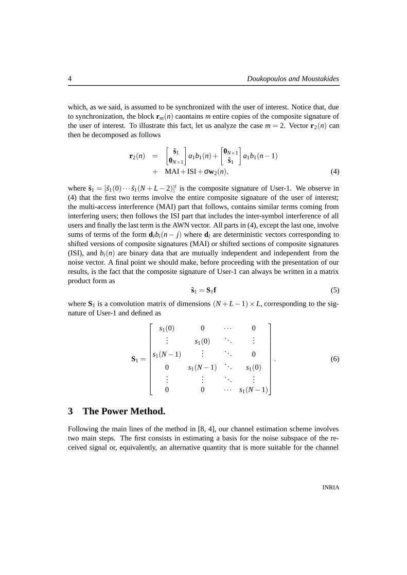
which, as we said, is assumed to be synchronized with the user of interest. Notice that, dueto synchronization, the block rm(n) caontains m entire copies of the composite signature ofthe user of interest. To illustrate this fact, let us analyze the case m = 2. Vector r2(n) canthen be decomposed as follows
r2(n) =
[s1
0N×1
]
a1b1(n)+
[0N×1
s1
]
a1b1(n−1)
+ MAI+ ISI+σw2(n), (4)
where s1 = [s1(0) · · · s1(N + L− 2)]t is the composite signature of User-1. We observe in(4) that the first two terms involve the entire composite signature of the user of interest;the multi-access interference (MAI) part that follows, contains similar terms coming frominterfering users; then follows the ISI part that includes the inter-symbol interference of allusers and finally the last term is the AWN vector. All parts in (4), except the last one, involvesums of terms of the form dlbi(n− j) where dl are deterministic vectors corresponding toshifted versions of composite signatures (MAI) or shifted sections of composite signatures(ISI), and bi(n) are binary data that are mutually independent and independent from thenoise vector. A final point we should make, before proceeding with the presentation of ourresults, is the fact that the composite signature of User-1 can always be written in a matrixproduct form as
s1 = S1f (5)
where S1 is a convolution matrix of dimensions (N + L− 1)×L, corresponding to the sig-nature of User-1 and defined as
S1 =
s1(0) 0 · · · 0... s1(0)
. . ....
s1(N −1)...
. . . 0
0 s1(N −1). . . s1(0)
......
. . ....
0 0 · · · s1(N −1)
. (6)
3 The Power Method.
Following the main lines of the method in [8, 4], our channel estimation scheme involvestwo main steps. The first consists in estimating a basis for the noise subspace of the re-ceived signal or, equivalently, an alternative quantity that is more suitable for the channel
INRIA
Blind Channel Estimation for DS-CDMA 5
estimation problem. The second step, once the information regarding the noise subspace isavailable, consists in estimating the final channel impulse response.
Let us first consider the autocorrelation matrix Rrm of the received data vector rm(n)defined in (3), then
Rrm
4= E{rm(n)rt
m(n)} = Q+σ2I (7)
where I is the identity matrix and Q a square matrix of dimension (mN +L−1) having theform
Q = ∑l
dldtl , (8)
with dl the deterministic vectors contributing to rm(n) defined in (4).Consider now the SVD of the matrix Q
Q = [Us Un]
[Λs 00 0
]
[Us Un]t ; (9)
this leads to the following SVD of the autocorrelation matrix Rrm
Rrm = [Us Un]
[Λs +σ2I 0
0 σ2I
]
[Us Un]t . (10)
where Λs is a diagonal matrix containing the singular values of Q and [Us Un] an orthonor-mal matrix with Us, Un being orthonormal bases for the signal and noise subspace respec-tively. We can see that the singular values of Rrm corresponding to the noise subspace areall equal to σ2 and are the smallest ones since the elements of Λs are positive. Using thedecomposition in (10) we can now state the next lemma which constitutes the main ideathat our method is based on.
Lemma 1 Let Rrm be the autocorrelation matrix defined in (7) and consider the SVD in(10), then we have the following limit
limk→∞
(σ2R−1
rm
)k= UnUt
n. (11)
Proof of Lemma 1:Let λ1 ≥ λ2 ≥ . . . ≥ λd > 0 be the diagonal elements of the matrix Λs, then we can write
(σ2R−1
rm
)k= [Us Un]
[(Λs+σ2I
σ2
)−k0
0 I
]
[Us Un]t . (12)
RR n° 4781
6 Doukopoulos and Moustakides
From the above equality we can see that the only term in the right hand side that depends
on the power k is the matrix(
Λs+σ2Iσ2
)−k. Since Λs+σ2I
σ2 is diagonal with elements of the formλi+σ2
σ2 > 1, for i = 1, . . . ,d, we may deduce that
limk→∞
(Λs +σ2I
σ2
)−k
= 0. (13)
Finally, combining (12) and (13) we can easily verify the validity of (11).
Lemma 1 is a variant of the power method [1] used in numerical analysis for estimatingthe subspace corresponding to the maximum singular value. Since σ2 is the smallest singu-lar value of Rrm , by considering the inverse matrix R−1
rmin the lemma, the noise subspace Un
is mapped to 1/σ2 which becomes the largest singular value of the inverse matrix. Our in-tention is to use the power R−k
rmfor approximating the product UnUt
n. Since, as we can see in(13), the speed of convergence is exponential with the slowest component being of the form(σ2/(λd +σ2))k, we can clearly deduce that the power method is more efficient in high SNRcases. In other words we expect in high SNR to approximate more efficiently the desiredproduct with smaller powers; a fact that will also become apparent in our simulations.
4 Key Results.
Channel estimation methods that use SVD of the autocorrelation matrix Rrm are based onthe following key idea. Since from SVD the matrix [Us Un] is orthonormal we have thatUt
nUs = 0. This suggests that for any vector s belonging to the signal subspace we also have
Utns = 0. (14)
In particular this is true for all vectors dl contributing to the matrix Q defined in (8). Wehave now the following lemma which is a straightforward consequence of (14).
Lemma 2 Let f denote the channel impulse response that we like to estimate; if F i, i =1, . . . , l, are matrices such that all vectors Fif belong to the signal subspace then
(UtnF)f = 0, where F = F1 + · · ·+Fl. (15)
From (15) it is clear that if we had available the exact noise subspace basis Un and amatrix F then we could recover f as a vector belonging to the null space of the matrix Ut
nF.
INRIA
Blind Channel Estimation for DS-CDMA 7
4.1 Identifiability.
In this subsection, we will briefly consider the problem of consistency of the channel im-pulse response estimates through (15). We must stress that identifiability issues are in gen-eral complicated; for a more rigorous analysis one can consult [3]. Here we would liketo adopt a rather simplistic approach that provides a better insight of the problem and alsoleads to necessary conditions.
Consider the autocorrelation matrix Rrm of dimensions (mN + L− 1)× (mN + L− 1)and the corresponding SVD of (10). Let us denote by rs, rn the signal and noise subspaceranks respectively, then the matrix Ut
nF in (15) is of dimensions rn ×L. If Un is the exactnoise subspace and F is a matrix such that Ff belongs to the signal subspace then we canconclude that, due to (15), the column rank of Ut
nF can, at most, be equal to L−1. In orderfor (15) to have a unique solution (modulo a multiplicative constant-ambiguity) the columnrank of Ut
nF must be exactly equal to L−1. Since the column rank of a matrix is equal to itsrow rank (and also equal to the rank of the matrix) we conclude that in order to have a rowrank equal to L−1 a necessary condition is to have at least L−1 rows, that is, rn ≥ L−1.Since rs + rn = mN +L−1 this yields the following necessary condition
rs ≤ mN. (16)
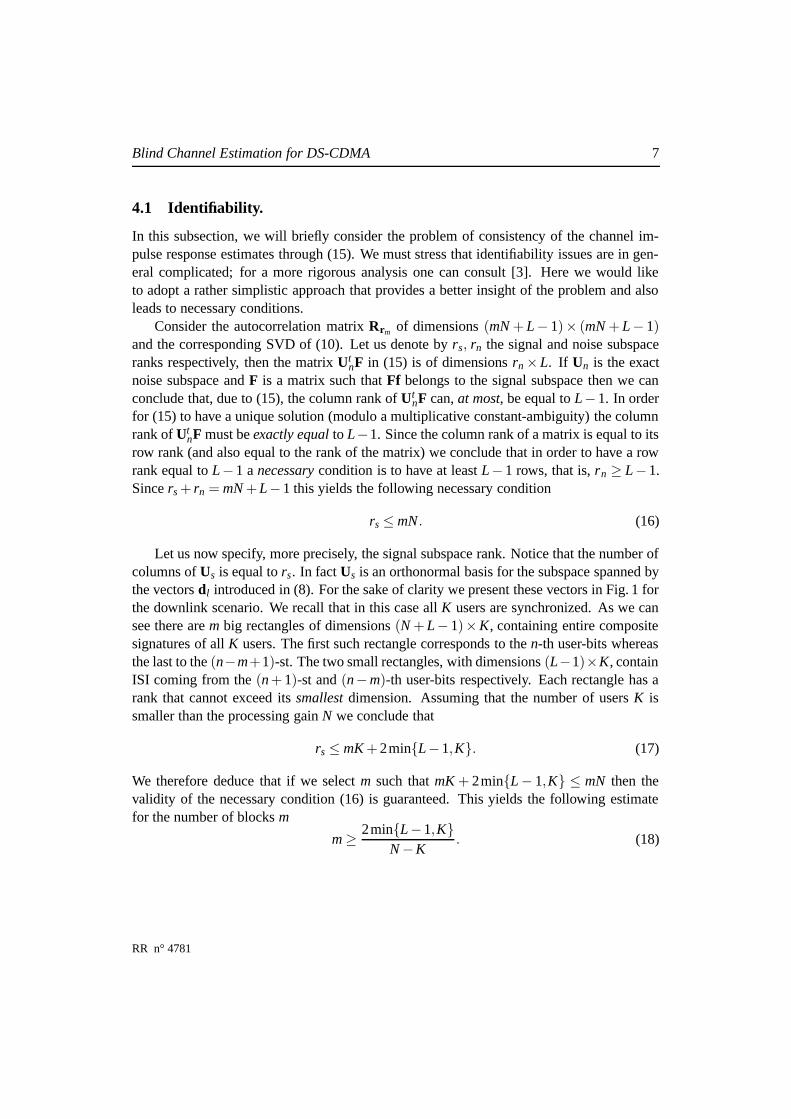
Let us now specify, more precisely, the signal subspace rank. Notice that the number ofcolumns of Us is equal to rs. In fact Us is an orthonormal basis for the subspace spanned bythe vectors dl introduced in (8). For the sake of clarity we present these vectors in Fig. 1 forthe downlink scenario. We recall that in this case all K users are synchronized. As we cansee there are m big rectangles of dimensions (N + L− 1)×K, containing entire compositesignatures of all K users. The first such rectangle corresponds to the n-th user-bits whereasthe last to the (n−m+1)-st. The two small rectangles, with dimensions (L−1)×K, containISI coming from the (n + 1)-st and (n−m)-th user-bits respectively. Each rectangle has arank that cannot exceed its smallest dimension. Assuming that the number of users K issmaller than the processing gain N we conclude that
rs ≤ mK +2min{L−1,K}. (17)
We therefore deduce that if we select m such that mK + 2min{L− 1,K} ≤ mN then thevalidity of the necessary condition (16) is guaranteed. This yields the following estimatefor the number of blocks m
m ≥2min{L−1,K}
N −K. (18)
RR n° 4781
8 Doukopoulos and Moustakides
(L−1)×K
(N +L−1)×K
(N +L−1)×K
••
•
(N +L−1)×K
(L−1)×K
Figure 1: Representation of the vectors composing the signal subspace.
Equivalently, for a given number of blocks m, we can obtain an upper bound for the maxi-mum load of the system
K ≤ N −2min
{N
m+2,
L−1m
}
. (19)
If we like to follow the same analysis for the uplink scenario then, due to lack of syn-chronization, relation (17) becomes rs ≤ (m+2)K, yielding
m ≥2K
N−Kor K ≤
mm+2
N (20)
as a possible estimate for m (for given K) or an upper bound for K (for given m). As wasstated before, a more rigorous analysis can be found in [3], addressing also the identifiabilityproblem in the case where for L we know only an upper bound. We must stress that thebounds introduced in (18) and (19) are by no means strict and must therefore be used withcaution. We recall that they simply ensure validity of the necessary condition (16) and are
INRIA
Blind Channel Estimation for DS-CDMA 9
thus not sufficient for identifiability. In numerous simulations, however, they turned out tobe very accurate. Unfortunately we were not able to prove their sufficiency.
4.2 Two Optimization Problems.
Let us now see how we can use Equ. (15) in combination with the power method introducedin Section III in order to solve the channel estimation problem. We first observe that any fsatisfying (15) also satisfies the following equation
ft FtUnUtnFf = 0. (21)
Furthermore, if for any vector h of length L, we define the nonnegative measure
V (h) = htFtUnUtnFh, (22)
then Equ. (21) suggests the following two optimization problems for recovering the channelimpulse response f.
The first method consists in solving the minimization problem
f = argminh
V (h); subject to ‖h‖ = 1. (23)
Thus f is being estimated as the singular vector corresponding to the smallest singular valueof the matrix FtUt
nUnF. We should note that the SVD problem suggested by (23) is only ofsize L (channel length).
The second method relies on a constrained least squares (LS) minimization. Morespecifically let
hi = arg minh
V (h); subject to htei = 1, (24)
where ei, i = 1, . . . ,M, are pre-specified vectors. The final candidate vector is the one thatis closest to the SVD solution, that is, f = hio/‖hio‖, where io is given by
io = argmini
V (hi)/‖hi‖2. (25)
In the ideal case when we have exact knowledge of the noise subspace, due to (21), theoptimum value V (f) of the criterion V (h) in both, SVD and LS approaches, becomes ex-actly zero. Moreover, for LS a single vector ei would suffice to exactly determine f. Whenhowever only estimates of the noise subspace are available, then the minimum value of thecriterion is positive and for LS we need to use more than one vectors ei in order to efficientlyapproximate the performance of the SVD solution (23). Finally we should note that the es-timates f that we obtain with both methods differ from the true f by a multiplicative constant
RR n° 4781
10 Doukopoulos and Moustakides
(multiplicative constant ambiguity). In fact if we assume (without loss of generality) thatthe norm of f is unity, then in the estimate f we have only a sign ambiguity.
Notice now that in both optimizations (23) and (24), it is the product UnUtn that appears
as part of the function V (h). As we have seen in Lemma 1 this quantity can be approxi-mated, to any degree, by the corresponding matrix power
UnUn = σ2kR−krm
(26)
yielding the following approximation for the measure V (h) defined in (22)
V (h) = σ2khtFtR−krm
Fh. (27)
Using V (h), the two optimization problems become
f = arg minh
V (h) = argminh
htFtR−krm
Fh; subject to ‖h‖ = 1, (28)
corresponding to the SVD version of (23); and
hi = argminh
V (h) = argminh
htFtR−krm
Fh; subject to htei = 1, (29)
with f = hio/‖hio‖ and io satisfying
io = arg mini
V (hi)/‖hi‖2 = arg min
iht
iFtR−k
rmFhi/‖hi‖
2, (30)
for the LS version of (24). If in particular in the LS problem we select ei = [0 · · ·010 · · ·0]t ,for i = 1, . . . ,L, with the unity being in the i-th position then (29) yields
hi =(Ft R−k
rmF)−1ei
eti(FtR−k
rm F)−1ei, (31)
and the final channel estimate becomes f = hio/‖hio‖, where
io = argmini
1
eti(Ft R−k
rm F)−1ei
= argmaxi
eti(F
tR−krm
F)−1ei (32)
It is more convenient to view the solution of the LS problem as first computing the inversematrix (Ft R−k
rmF)−1, then selecting its largest diagonal element whose position identifies io;
the final channel estimate is then the io-th row (or column) of (FtR−krm
F)−1 normalized tounit norm.
INRIA
Blind Channel Estimation for DS-CDMA 11
Notice that although for the approximation of the product UnUtn through Lemma 1 we
need σ2, this quantity plays absolutely no role in the estimation of f through (28) or (29).Another interesting point is the fact that for this approximation no knowledge of the noisesubspace rank is necessary. This should be compared to the large SVD applied to Rrm in[8, 4] where for the determination of Un, the knowledge of this parameter (or a reliableestimate) is indispensable.
5 Channel Estimation Method and Synchronization.
In this section we probe further into our problem by exploiting the special structure of thedl-vectors introduced in (8) that correspond to the user of interest. For the application of thetwo estimation schemes (SVD and LS) presented in the previous section, we need to have aknown matrix F such that Ff belongs to the signal subspace. It turns out that such a matrixis easy to obtain. For illustration let us again consider the case m = 2. From (4) we havethat the two vectors [st
1 01×N ]t and [01×N st1]
t belong to the signal subspace and, using (5),they can be written under the form Fif, i = 1,2, where
F1 =
[S1
0N×L
]
, F2 =
[0N×L
S1
]
. (33)
Since we assume that the signature of the user of interest is known, we conclude that bothmatrices Fi, i = 1,2 are known as well and so is their sum F = F1 +F2. This property canbe generalized to the m-block case in a straightforward manner and we can write
F =m−1
∑l=0
0lN×L
S1
0(m−1−l)N×L
. (34)
Matrix F turns out to have a simple structure. In particular, it is a convolution matrix as in(6), but of dimensions (mN + L− 1)×L, where the first column contains the signature s1
repeated m times, i.e. it is of the form [
m times︷ ︸︸ ︷
st1 · · · st
1 01×L−1]t .
Since we have available a known F matrix we can now proceed to the computation ofthe autocorrelation matrix. We can approximate Rrm by using the sample autocorrelationmatrix of the received data vector, namely
Rrm =1T
T
∑n=1
rm(n)rtm(n). (35)
RR n° 4781
12 Doukopoulos and Moustakides
Thus we have now available all necessary parameters in order to solve the two optimizationproblems in (28) and (32).
Remark: A subtle and very important remark regarding Lemma 1 concerns the employ-ment of possible values for the power k. Notice that the limit in (11) is correct, i.e. we obtainthe product UnUt
n, only when the singular values corresponding to the noise subspace areexactly equal. Unfortunately, with the approximation in (35) this is rarely the case. Thisobservation leads to a twofold deduction. First, considering that the number of bits T isconstant, the employment of continuously increasing powers k does not necessarily lead toimproved performance. This is because the corresponding limit (11) instead of being thedesired product will become just the rank-one matrix uut where u is the singular vectorcorresponding to the smallest singular value of Rrm . On the other hand, for any two con-stant powers, as the number of bits T grows, eventually the larger power will prevail. In thesimulations section we will have the opportunity to confirm these observations.
Our proposed versions are clearly blind since they require only the received data se-quence rm(n) and knowledge of the signature s1 of the user of interest. We should alsonote that computing the product UnUt
n with the power method can be computationally veryefficient and even lead to on-line adaptive implementations. Although this is not a subjectthat we would like to raise here, since it is still under investigation, we can easily see that byadapting the inverse of the sample autocorrelation matrix Rrm using RLS, we immediatelygain an order of magnitude in computations as compared to applying directly SVD at eachstep. This is true because, as we shall see in the simulations, in order for our versions tomatch the performance of SVD we do not need to use powers beyond k = 3.
As was previously indicated, in [8, 4], where the matrix Un is estimated instead, thereis also the need to reliably identify the rank of the noise subspace. Such estimates are per-formed with the help of Akaike’s information criterion or the minimum description lengthcriterion (for details see [8]). Unfortunately, it turns out that, the schemes in [8, 4] tend to bevery sensitive with respect to the exact knowledge of the noise subspace rank. In particular,they can exhibit considerable performance degradation even when the corresponding esti-mate is slightly erroneous, as we will have the chance to find out in the next section. Finallywe should note that the method proposed in [6] coincides with our SVD version with thespecial selection k = 1. Although this specific choice provides efficient channel estimatesin high SNR, for medium to low SNR cases, significant performance gains can be obtainedby employing higher powers.
5.1 Synchronization.
Up to this point we assumed that the receiver, more precisely the data blocks rm(n), weresynchronized with the user of interest. Now we are going to relax this assumption and
INRIA
Blind Channel Estimation for DS-CDMA 13
propose a simple and efficient means for synchronization. We recall that the initial delay τof User-1 can take any value in the set {0, . . . ,N −1}.
Following the idea introduced in [4], we observe that when the second order statisticsare available (ideal case) and the block rm(n) is synchronized with the user of interestedthen, in both approaches (SVD and LS), the optimum value of the measure V (h) is equalto zero. When on the other hand the data block is not synchronized, the optimum value ofthe measure cannot attain this lower limit since Equ. (15) is no longer valid. In other wordsthe optimum value of V (h), as a function of the data block timing, is minimized when thedata block rm(n) is synchronized with the user of interest. This is exactly the property weare going to use to perform synchronization. In other words we propose to solve either theSVD or the LS minimization problem for all N possible timing values of the data block. Wecan then select as the estimate of the initial delay the one with the smallest optimum V (h)value.
A notable characteristic of the N minimizations involved in the synchronization problemis the fact that the (sample) autocorrelation matrices for consecutive delay values have asignificant overlap. By exploiting this property we will now present an efficient method forcomputing certain matrices entering in the two optimization problems. Let us denote byrm(n,τ) the following vector of length mN +L−1
rm(n,τ) = [y(nN − τ) · · ·y((n−m)N−L+2− τ)]t , (36)
where we have introduced a delay parameter τ. We can now, similarly to (35), define thecorresponding sample autocorrelation matrix as follows
Rτ =1T
T
∑n=1
rm(n,τ)rtm(n,τ), (37)
where for the sake of simplicity, we have not included the index rm in the definition in(37). One may easily observe that between the two matrices Rτ, Rτ+1 for any 0 ≤ τ ≤ N−2there is a square overlap of dimensions mN + L− 2. This is shown more clearly from thefollowing relation
Dτ =
[Rτ aτat
τ bτ+mN+L
]
=
[bτ bt
τbτ Rτ+1
]
, (38)
RR n° 4781
14 Doukopoulos and Moustakides
where
bν =1T
T
∑n=1
y2(nN −ν), (39)
aτ =1T
T
∑n=1
rm(n,τ)y((n−m)N −L+1− τ), (40)
bτ =1T
T
∑n=1
rm(n,τ+1)y(nN − τ). (41)
Using the Schur inverse complement [2] one can compute the matrix R−1τ+1, from R−1
τwith a rank-two modification. We first compute D−1
τ as follows
D−1τ =
[R−1
τ 00t 0
]
+1p1
[y1
][yt 1
], (42)
where
p1 = bτ+mN+L −atτR−1
τ aτ, (43)
y = −R−1τ aτ. (44)
Then, based on (38), we can obtain R−1τ+1 from D−1
τ from the relation
[0 0t
0 R−1τ+1
]
= D−1τ −
1p2
[1x
][1 xt], (45)
where
p2 =b2
τ
bτ +[0 bt
τ]
D−1τ
[0bτ
] , (46)
[0x
]
= −
(
p2
bτ
)
D−1τ
[0bτ
]
. (47)
Computing R−1τ+1 from the R−1
τ requires O((mN +L−1)2) operations while computingthe inverse directly has complexity O((mN + L− 1)3); thus gaining an order of magnitudein operations.
INRIA
Blind Channel Estimation for DS-CDMA 15
6 Simulations - Discussion.
In this section, we perform several simulations to demonstrate the satisfactory performanceof the blind channel estimation schemes developed in the previous section. We focus on thedownlink scenario, and consider various cases according to the size of the processing gain.More specifically, we examine the performance of our algorithms for signature waveformsof length N = 16 and N = 128 under diverse signaling conditions. Since the methods de-veloped in [8, 4] present very similar performances we will compare our schemes only to[8]. Furthermore, regarding the estimation scheme of [6], we recall that it coincides withour SVD, k = 1 version. We first proceed with spreading codes of N = 16 and then continueto the N = 128 case.
6.1 Spreading Codes of Length 16.
Randomly generated sequences of length N = 16 are used as spreading codes. Once gen-erated, the codes are kept constant for the whole simulation set. We use the length L = 3channel of [5] (known to be a “difficult case” due to the deep null in its frequency response).The number of blocks that are processed together is m = 3. This selection, according to (19),allows the load of the system to go up to 14 users. For our simulations we select K = 10users. User-1 is assumed to be the user of interest having unit power. All other users areassumed to have the same power level, which is 20 db higher than User-1.
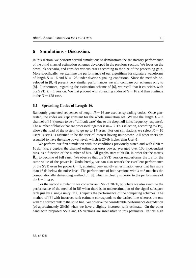
We perform our first simulation with the conditions previously stated and with SNR =10 db. Fig. 2 depicts the channel estimation error power, averaged over 100 independentruns, as a function of the number of bits. All graphs start at bit 50, in order for the matrixRr3 to become of full rank. We observe that the SVD version outperforms the LS for thesame value of the power k. Undoubtedly, we can also remark the excellent performanceof the SVD even for power k = 1, attaining very rapidly an estimation error that lies morethan 15 db below the noise level. The performance of both versions with k = 3 matches thecomputationally demanding method of [8], which is clearly superior to the performance ofthe k = 1 case.
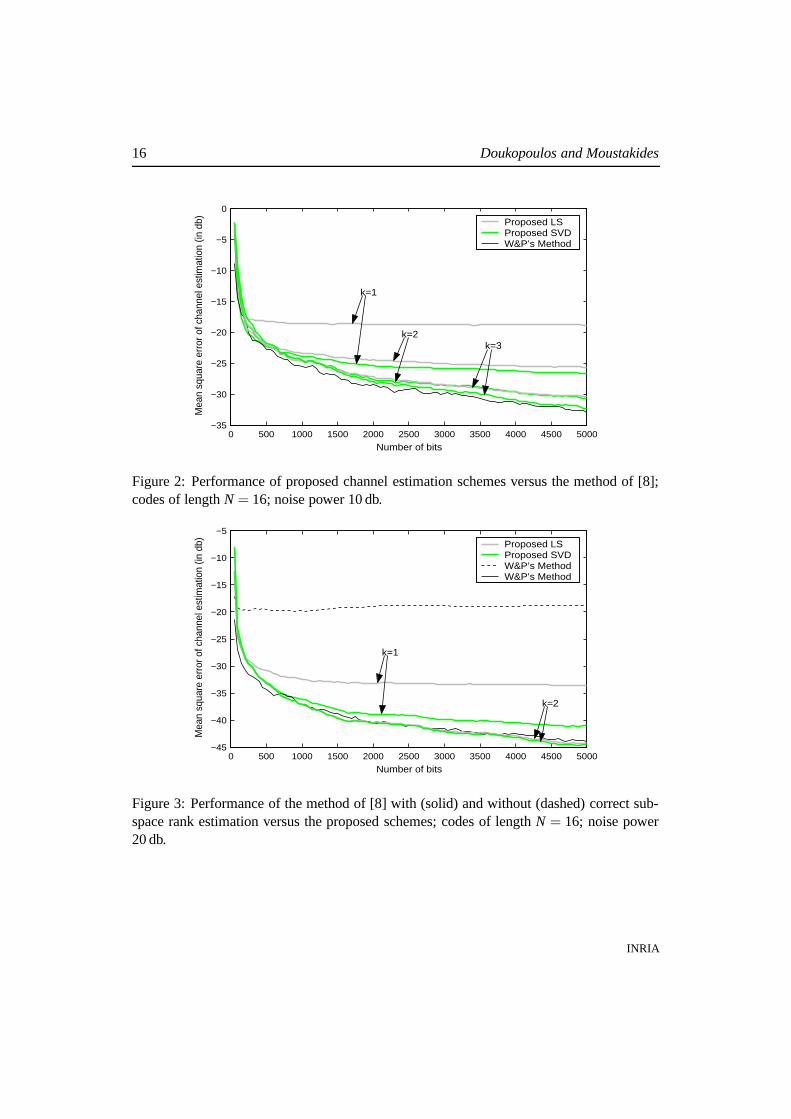
For the second simulation we consider an SNR of 20 db, only here we also examine theperformance of the method in [8] when there is an underestimation of the signal subspacerank just by a single unity. Fig. 3 depicts the performance of the competing schemes. Themethod of [8] with incorrect rank estimate corresponds to the dashed line whereas the onewith the correct rank to the solid line. We observe the considerable performance degradation(of approximately 25 db) when we have a slightly incorrect rank estimate. On the otherhand both proposed SVD and LS versions are insensitive to this parameter. In this high
RR n° 4781
16 Doukopoulos and Moustakides
0 500 1000 1500 2000 2500 3000 3500 4000 4500 5000−35
−30
−25
−20
−15
−10
−5
0
Number of bits
Mea
n sq
uare
err
or o
f cha
nnel
est
imat
ion
(in d
b) Proposed LSProposed SVDW&P’s Method
k=1
k=2 k=3
Figure 2: Performance of proposed channel estimation schemes versus the method of [8];codes of length N = 16; noise power 10 db.
0 500 1000 1500 2000 2500 3000 3500 4000 4500 5000−45
−40
−35
−30
−25
−20
−15
−10
−5
Number of bits
Mea
n sq
uare
err
or o
f cha
nnel
est
imat
ion
(in d
b) Proposed LSProposed SVDW&P’s MethodW&P’s Method
k=1
k=2
Figure 3: Performance of the method of [8] with (solid) and without (dashed) correct sub-space rank estimation versus the proposed schemes; codes of length N = 16; noise power20 db.
INRIA
Blind Channel Estimation for DS-CDMA 17
SNR environment, we can also see that their performance is maximized with k = 2. Again,all graphs are the result of an average of 100 independent runs.
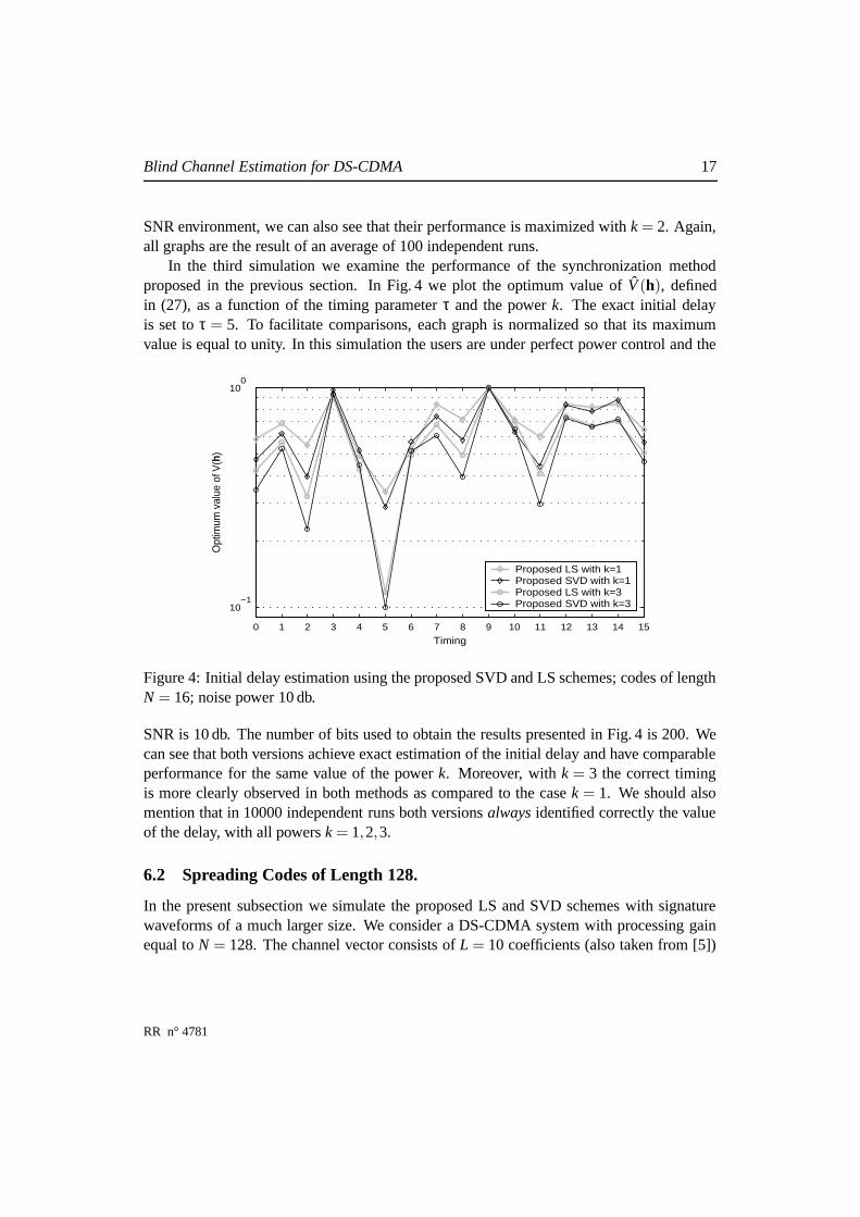
In the third simulation we examine the performance of the synchronization methodproposed in the previous section. In Fig. 4 we plot the optimum value of V (h), definedin (27), as a function of the timing parameter τ and the power k. The exact initial delayis set to τ = 5. To facilitate comparisons, each graph is normalized so that its maximumvalue is equal to unity. In this simulation the users are under perfect power control and the
0 1 2 3 4 5 6 7 8 9 10 11 12 13 14 15
10−1
100
Timing
Opt
imum
val
ue o
f V(h
)
Proposed LS with k=1Proposed SVD with k=1Proposed LS with k=3Proposed SVD with k=3
Figure 4: Initial delay estimation using the proposed SVD and LS schemes; codes of lengthN = 16; noise power 10 db.
SNR is 10 db. The number of bits used to obtain the results presented in Fig. 4 is 200. Wecan see that both versions achieve exact estimation of the initial delay and have comparableperformance for the same value of the power k. Moreover, with k = 3 the correct timingis more clearly observed in both methods as compared to the case k = 1. We should alsomention that in 10000 independent runs both versions always identified correctly the valueof the delay, with all powers k = 1,2,3.
6.2 Spreading Codes of Length 128.
In the present subsection we simulate the proposed LS and SVD schemes with signaturewaveforms of a much larger size. We consider a DS-CDMA system with processing gainequal to N = 128. The channel vector consists of L = 10 coefficients (also taken from [5])
RR n° 4781
18 Doukopoulos and Moustakides
and the number of blocks processed together is, as before, m = 3. The load upper boundfrom (19) becomes 121 users. The total number of users considered here is K = 80, with 29of them having the same power as User-1; 30 users being 10 db stronger; and the remaining20 being 20 db stronger than the user of interest. Again all graphs are the average of 100independent runs.
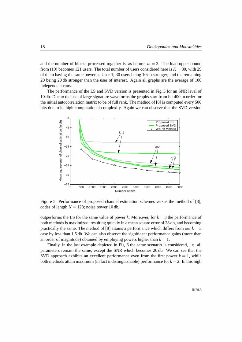
The performance of the LS and SVD version is presented in Fig. 5 for an SNR level of10 db. Due to the use of large signature waveforms the graphs start from bit 400 in order forthe initial autocorrelation matrix to be of full rank. The method of [8] is computed every 500bits due to its high computational complexity. Again we can observe that the SVD version
0 500 1000 1500 2000 2500 3000 3500 4000 4500 5000−35
−30
−25
−20
−15
−10
−5
0
Number of bits
Mea
n sq
uare
err
or o
f cha
nnel
est
imat
ion
(in d
b) Proposed LSProposed SVDW&P’s Method
k=1
k=2
k=3
Figure 5: Performance of proposed channel estimation schemes versus the method of [8];codes of length N = 128; noise power 10 db.
outperforms the LS for the same value of power k. Moreover, for k = 3 the performance ofboth methods is maximized, resulting quickly in a mean square error of 28 db, and becomingpractically the same. The method of [8] attains a performance which differs from our k = 3case by less than 1.5 db. We can also observe the significant performance gains (more thanan order of magnitude) obtained by employing powers higher than k = 1.
Finally, in the last example depicted in Fig. 6 the same scenario is considered, i.e. allparameters remain the same, except the SNR which becomes 20 db. We can see that theSVD approach exhibits an excellent performance even from the first power k = 1, whileboth methods attain maximum (in fact indistinguishable) performance for k = 2. In this high
INRIA
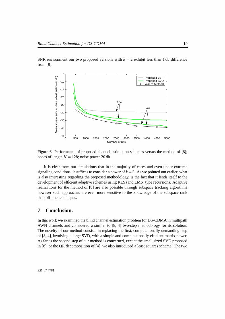
Blind Channel Estimation for DS-CDMA 19
SNR environment our two proposed versions with k = 2 exhibit less than 1 db differencefrom [8].
0 500 1000 1500 2000 2500 3000 3500 4000 4500 5000−45
−40
−35
−30
−25
−20
−15
−10
−5
Number of bits
Mea
n sq
uare
err
or o
f cha
nnel
est
imat
ion
(in d
b) Proposed LSProposed SVDW&P’s Method
k=1
k=2
Figure 6: Performance of proposed channel estimation schemes versus the method of [8];codes of length N = 128; noise power 20 db.
It is clear from our simulations that in the majority of cases and even under extremesignaling conditions, it suffices to consider a power of k = 3. As we pointed out earlier, whatis also interesting regarding the proposed methodology, is the fact that it lends itself to thedevelopment of efficient adaptive schemes using RLS (and LMS) type recursions. Adaptiverealizations for the method of [8] are also possible through subspace tracking algorithmshowever such approaches are even more sensitive to the knowledge of the subspace rankthan off line techniques.
7 Conclusion.
In this work we examined the blind channel estimation problem for DS-CDMA in multipathAWN channels and considered a similar to [8, 4] two-step methodology for its solution.The novelty of our method consists in replacing the first, computationally demanding stepof [8, 4], involving a large SVD, with a simple and computationally efficient matrix power.As far as the second step of our method is concerned, except the small sized SVD proposedin [8], or the QR decomposition of [4], we also introduced a least squares scheme. The two
RR n° 4781
20 Doukopoulos and Moustakides
versions (LS and SVD) were tested under diverse signaling conditions and always comparedvery favorably to the methods of [8, 4] but at a significantly lower computational cost.Unlike however the latter methods, our approach does not require any a-priori knowledge orestimates of the signal subspace rank, since it is completely independent of this parameter.As far as the approach in [6] is concerned, we should mention that it coincides with ourSVD version with k = 1. Here however, by employing higher powers of k, we can obtainsuperior performance especially in medium to low SNR environments.
Finally, both proposed versions were also extended in order to allow for synchronizationwith the user of interest. In particular by exploiting the special structural characteristics ofthe synchronization problem, we developed an efficient scheme that reduces the complexityof the most computationally demanding part, by an order of magnitude.
References
[1] G.H. Golub and C.F. Van Loan, Matrix Computations, 2nd edn, The John Hopkins University Press,1990.
[2] T. Kailath. Linear Systems, Prentice Hall, 1980.
[3] P. Loubaton and E. Moulines, ”On blind multiuser forward link channel estimation by the subspacemethod: Identifiability results,” IEEE Trans. on Signal Processing, vol. 48, pp. 2366-2376, Aug. 2000.
[4] Z. Pi and U. Mitra, “On blind timing acquisition and channel estimation for wideband multiuser DS-CDMA systems,” special issue on multiuser detection, Journal of VLSI Signal Processing, vol. 30, pp.127-142, 2002.
[5] J.G. Proakis, Digital Communications, 4-th Edition, McGraw-Hill, New York, 2001.
[6] M.K. Tsatsanis and Z. Xu, “Performance Analysis of minimum variance CDMA receivers,” IEEE Trans.on Signal Processing, vol. 46, pp. 3014-3022, Nov. 1998.
[7] S. Verdú, Multiuser Detection, Cambridge University Press, New York, 1998.
[8] X. Wang and H.V. Poor, “Blind equalization and multiuser detection in dispersive CDMA channels,”IEEE Trans. on Communications, vol. 46, pp. 91-103, Jan. 1998.
[9] Z. Xu and M.K. Tsatsanis, “Blind adaptive algrithms for minimum variance CDMA receivers,” IEEETrans. on Communications, vol. 49, pp. 180-194, Jan. 2001.
[10] Z. Xu and P. Liu “Kurtosis based maximization/minimization approach to blind equalization forDS/CDMA systems in unknown multipath,” IEEE ICASSP2002, Orlando, vol. III, pp. 2585-2588, 2002.
INRIA

Unité de recherche INRIA RennesIRISA, Campus universitaire de Beaulieu - 35042 Rennes Cedex (France)
Unité de recherche INRIA Lorraine : LORIA, Technopôle de Nancy-Brabois - Campus scientifique615, rue du Jardin Botanique - BP 101 - 54602 Villers-lès-Nancy Cedex (France)
Unité de recherche INRIA Rhône-Alpes : 655, avenue de l’Europe - 38330 Montbonnot-St-Martin (France)Unité de recherche INRIA Rocquencourt : Domaine de Voluceau - Rocquencourt - BP 105 - 78153 Le Chesnay Cedex (France)
Unité de recherche INRIA Sophia Antipolis : 2004, route des Lucioles - BP 93 - 06902 Sophia Antipolis Cedex (France)
ÉditeurINRIA - Domaine de Voluceau - Rocquencourt, BP 105 - 78153 Le Chesnay Cedex (France)
http://www.inria.frISSN 0249-6399