SIAM J. APPLIED DYNAMICAL SYSTEMS c© 2005 Society for Industrial and Applied MathematicsVol. 4, No. 1, pp. 159–186

Blinking Rolls: Chaotic Advection in a Three-Dimensional Flow with an Invariant∗

P. Mullowney†, K. Julien†, and J. D. Meiss†

Abstract. We study a simple, nonautonomous, three-dimensional, incompressible flow corresponding to sequen-tially active two-dimensional rolls with distinct axes. A feature of the model is that an analytical mapis obtained. We show that when the roll axes are orthogonal, motion is confined to two-dimensionaltopological spheres. The dynamics on each surface ranges from nearly regular to largely chaotic.We study the transport and mixing on each surface and their dependence upon parameters in thesystem.

Key words. chaotic advection, transport, mixing, volume-preserving mappings

AMS subject classifications. 76F25, 37B55, 70K55, 37D45

DOI. 10.1137/040606727

1. Introduction. Fluid mixing corresponds to the transport of passive scalars by kine-matic advection and their subsequent diffusive homogenization. Such phenomena are funda-mentally important in many physical systems and engineering applications [36] and occur ata variety of scales ranging from the very small (micrometer scale) to the very large (plan-etary scales and beyond). For instance, mixing in microchannels can be used to efficientlyhomogenize reagents in chemical reactions even when the flow is laminar [41]. Understandingtransport for planetary scale flows is critical for climate modeling and pollution dispersionin atmospheric science [8] and eddy dynamics in oceanography [23]. Transport and mixingare also important in granular flows [33], population biology [32, 39], and reaction-diffusionsystems [35].

The mixing of tracer particles in a fluid flow is due to a combination of stirring and diffu-sion. In an efficient mixing process, stirring rapidly transports tracer elements by kinematicadvection throughout the domain. The associated stretching and folding of material lines andsurfaces ultimately trigger diffusive processes that homogenize the tracers into a blended mix-ture. Originally, it was assumed that mixing was most important in the context of turbulentflows where both processes are evident. However, as is now well known, effective mixing alsooccurs in laminar flows [2].

In three dimensions, these problems are especially challenging from a theoretical stand-point. One of the earliest advances came with the work on the Arnold–Beltrami–Childress(ABC) flow [13], an exact solution to the Euler equations. It was found that efficient stir-ring in three-dimensional incompressible flows can occur even for laminar and autonomous

∗Received by the editors April 14, 2004; accepted for publication (in revised form) by M. Golubitsky July 18,2004; published electronically February 22, 2005.

http://www.siam.org/journals/siads/4-1/60672.html†Department of Applied Mathematics, University of Colorado, Boulder, CO 80309-0526 (paul.mullowney@

colorado.edu, julien@colorado.edu, jdm@colorado.edu). The first author was supported by NSF VIGRE grant DMS-9810751. The second author was supported by an NSF grant OCE-0137347. The third author was supported inpart by NSF grant DMS-0202032.

159

160 P. MULLOWNEY, K. JULIEN, AND J. D. MEISS

Eulerian velocity fields. Although the ABC flow is probably not physically observable, thecrucial idea is that mixing can occur even in the simplest of flows in three dimensions [36].In the two-dimensional case, transport can also be achieved in laminar, time-dependent flows.One of the seminal models was developed by Aref, who coined the term “chaotic advection”[1]. His flow, called the “blinking vortex,” is specifically designed to yield nonintegrable La-grangian trajectories. This model can be interpreted as an idealized mixing protocol wherepassive tracers are successively captured by the velocity fields of vortical stirrers that are theanalogues of turbulent eddies with finite lifetimes.

In sections 2 and 3, we generalize the blinking vortex model and construct a physicallymotivated, yet mathematically simple, system with three-dimensional mixing. Our model,which we call “blinking rolls,” replaces Aref’s alternatively active vortices with alternativelyactive arrays of rolls aligned in different directions.

Though our mixing protocol is idealized, there is experimental evidence for the existenceof similar flows. One such example is observed in Rayleigh–Benard convection experimentsfor a binary mixture in a square cell with insulating sides. When the vertical temperaturedifference exceeds a threshold value, an instability leads to a sequence of temporally alter-nating, orthogonal convection rolls whose axes are parallel to the square boundaries [34]. Itis observed that “the transition from one set of rolls to the other is very fast, followed by arelatively long period of domination by one of the rolls . . . the system lies most of the timein the roll patterns.” Another example of roll-switching is the Kuppers–Lortz instability forrotating convection in a pure fluid [28, 9, 43, 22, 42]. Rotation causes an instability thatresults in switching of the roll axes by roughly 60◦. Theoretical and experimental studieshave shown that the rolls switch with a characteristic frequency proportional to the relativetemperature difference above threshold.

When the switching occurs much faster than the roll turnover time, it can be idealized asinstantaneous. In this case, the flow can be viewed as a composition of maps correspondingto the action of each individual roll. For the incompressible case, this gives a compositionof volume-preserving maps. Transport in volume-preserving maps was studied in pioneeringwork on a discretized ABC system [37, 15, 12, 11]. The onset of transport is closely related tothe destruction of heteroclinic connections for codimension-one manifolds [38, 29]; a Melnikovmethod was developed to study the bifurcations in manifold crossings in [30, 31].

It is generally difficult to find models for three-dimensional flows that both are math-ematically accessible and have effective transport. However, there is a small but growinglink between mixing in experimental, three-dimensional flows and theoretical modeling basedon chaotic advection. Shinbrot and his collaborators have studied the transient behavior ofweakly buoyant tracers in a laminar flow within a cylindrical batch stirring device using atraveling wave map with a buoyancy term [40]. In a similar though less symmetric device,a close link was found between the invariant regions of the flow visualized with a sheet laserand fluorescent dyes and the corresponding island chains of the Poincare sections of a model[18, 19]. These examples reflect the growing evidence that mixing in three-dimensional flowscan be effectively modeled via chaotic advection [36, 2]. This is crucial because it allows one totreat the flow as a low-dimensional dynamical system and thus bring to bear the geometricaland qualitative tools of dynamical systems theory.

In this paper, we present a theoretical and computational analysis for the blinking roll

BLINKING ROLLS 161

model. In section 2 the flow for a single roll is constructed and the equations of motion aresolved to obtain an analytical time-t map. In section 3 the flow with roll-switching is modeledby composing several of these maps. For the case that the roll axes are orthogonal, thereis an invariant that constrains the motion to two-dimensional surfaces. In fact, we show insection 4 that the invariant persists regardless of the choice of stirring protocol. This systemhas a number of symmetries that simplify its analysis; see section 5. In section 6, we usenormal form expansions to understand behavior near a fixed point and near roll boundaries.Numerical results are given in section 7.

2. Blinking rolls. Aref’s blinking vortex flow corresponds to a two-dimensional, inviscid,incompressible fluid in a circular domain of radius a [1]. A point vortex moves inside thebounding contour according to a stirring protocol (x(t), y(t)). The equations for a passivescalar in such a fluid are Hamiltonian, and if the vortex position is constant in either a fixedor a steadily rotating coordinate system, then the flow is integrable. Otherwise, the flow istypically nonintegrable.

The blinking vortex corresponds to a stirring protocol with period T . For the first half ofthe period, a vortex resides at (b, 0), and for the remainder of the period a vortex resides at(−b, 0) for some b < a. For simplicity it is assumed that there is an instantaneous transitionbetween the flows associated with the finite-lifetime point vortices. This allows the equations ofmotion for each half period to be solved exactly, giving rise to the half period maps F1(x, y) andF2(x, y). The Lagrangian tracer dynamics is then governed by the full period map f = F2◦F1.

Two-dimensional transport can then be studied simply by iterating the map. The dynam-ics are governed by two dimensionless parameters µ = ΓT

2πa2 , representing the vortex strength,

and β = ba , its relative radial position. If β is held fixed, then, for small enough µ, chaotic

advection is localized and there is no global transport. As µ increases, the chaotic regionsgrow and the phase portrait becomes increasingly homogenized.

Here we will construct a three-dimensional model analogous to the blinking vortex system.The model consists of flows generated by a succession of two-dimensional “rolls” aligned indistinct directions that are applied for alternating time intervals. By “roll,” we mean thecirculating flow associated with a vortical tube where the vorticity vector and the tube axisare aligned. We do not consider drift along the roll axes. The flow is thus invariant along theroll axis and can be represented in terms of a stream function ψ with corresponding velocityfield

v = ∇ψ(x⊥, t) × e‖,(1)

where e‖ is the unit vector in the invariant direction. This generates motion in the x⊥-planenormal to e‖; if ψ is autonomous, this motion is also confined to a two-dimensional surfacedefined by ψ constant. Any critical point of the stream function, i.e., a point where ∇ψ = 0,corresponds to a stationary axis. Near such an axis the flow is rotational whenever the criticalpoint is an extrema; the circulation near such an axis corresponds to a roll.

We will primarily study the case of an array of trigonometric rolls; when they are alignedin the x direction the stream function is given by

ψ = A cos(y) cos(z).(2)

162 P. MULLOWNEY, K. JULIEN, AND J. D. MEISS

This gives the velocity field

(x, y, z) = ∇ψ(y, z) × ex = (0,−A cos(y) sin(z), A sin(y) cos(z)).(3)

For this case, the line (y, z) = (0, 0) is a roll axis (as are the axes (mπ, nπ) for m,n ∈ Z);nearby orbits lie on topological circles enclosing x-axis; see Figure 1. These circles limit ona square as y and z approach ±π

2 . The line (y, z) = (π2 ,π2 ) and its translations by (mπ, nπ)

correspond to saddle equilibria. Indeed the square cylinder boundary of the set {|y|, |z| ≤ π2 }

consists of the stable and unstable manifolds of the saddles, and it bounds the roll surroundingthe x-axis by heteroclinic connections. If A > 0, the direction of rotation for this roll is right-handed or positive. If we translate by π in a single direction, the direction of rotation becomesleft-handed or negative.

Figure 1. Flow of a two-dimensional roll, ψ1(y, z), with positive rotation about the x-axis.

A system of blinking rolls is obtained by alternatively switching between rolls alignedin different directions. A general mixing protocol can be implemented through a randomspecification of array lifetimes, amplitudes, and phases. However, for simplicity and as apreliminary investigation we restrict ourselves to roll arrays that are confined to a periodiclattice.

For example, consider three different roll arrays defined by stream functions ψi, i = 1, 2, 3,and axes ei aligned with the unit vectors of a Cartesian coordinate system. Each roll has acorresponding velocity field vi analogous to (3). Specifically, suppose that the roll ψ3 is activefor 0 ≤ t < T3, ψ2 for T3 ≤ t < T3 +T2, and ψ1 for T3 +T2 ≤ t < T3 +T2 +T1. We repeat thisprocess periodically, so that the velocity field is time-periodic with period T = T1 + T2 + T3.While any one roll array, say, ψi, is active, the motion is integrable, since ψi is constant andis confined to a plane of constant xi. However, as each roll array acts successively, one wouldexpect that the trajectories should explore a fully three-dimensional domain.

More generally, we could allow the array of rolls to have arbitrary, multiplicative time

BLINKING ROLLS 163

dependence, giving the general velocity field

v(x, t) = A(t)∇ψ1 × e1 + B(t)∇ψ2 × e2 + C(t)∇ψ3 × e3.(4)

When A(t), B(t), and C(t) are arbitrarily chosen, it is presumably impossible to solve explicitlyfor the flow. The blinking roll case corresponds to the choice of alternating step functionsfor A(t), B(t), and C(t); see Figure 2. If we fix the functions ψi, then this system has sixparameters, the times, T1, T2, and T3, and the amplitudes of the step functions A, B, and C.The amplitudes of the roll arrays are analogous to the eddy strength Γ in Aref’s model.

C

T3

tT TT T1 12 23

A

BC(t) C(t)

A(t) A(t)

B(t) B(t)

T

Figure 2. Step functions A(t), B(t), and C(t).

Since only one roll array is active at any given time, if we can obtain an explicit solutionfor the flow of ψi, then we can construct an explicit time-t map during the period that onearray is active. We denote the time-Ti map for the stream function ψi by Fi:

Fi(x, y, z) = ΦTi(x, y, z) ,d

dtΦt = vi(Φt) , Φ0 = id.(5)

Here, the index i of Fi denotes the axis of rotation and the fixed direction under the map aswell as the time of activation Ti. The blinking roll map is the composition of these maps:

(x′, y′, z′) = F1 ◦ F2 ◦ F3(x, y, z) .(6)

Our next task is to obtain the explicit solutions for the flow in the case of (2).

3. Blinking roll map. In this section we construct the three-dimensional map for thevelocity field (4) with rolls defined by (2) and amplitudes given by Figure 2. We begin bysolving for the flow of a single roll to obtain an explicit time-t map. Composition of the mapsfor each ψi gives the full three-dimensional map (6).

The solution of the differential equations (3) can be easily obtained by noting that trajec-tories must satisfy dy

v2= dz

v3. The equations can be easily integrated in terms of Jacobi elliptic

164 P. MULLOWNEY, K. JULIEN, AND J. D. MEISS

functions [10] to obtain the flow

Φt

⎛⎝ x

yz

⎞⎠ =

⎛⎝ x

sin−1(ksn(At−M(y, z), k))sin−1(ksn(At + N(y, z), k))

⎞⎠ ,(7)

where the elliptic function modulus is

k =√

1 − cos2(y) cos2(z) .(8)

The functions M(y, z) and N(y, z) are defined by setting t = 0 to get the initial condition,e.g., sin y = −ksn(M,k) and sin(z) = ksn(N, k). Though solving for M and N appears torequire inversion of the elliptic functions, a much simplified expression that does not requirethis can be obtained by expanding sn using the sum formula [10]

sn(α + β) =sn(α)cn(β)dn(β) + sn(β)cn(α)dn(α)

1 − k2sn2(α)sn2(β).

Note that the time t and amplitude A occur only in the combination At in (7). Thusif we rescale time by setting T = At, then we can eliminate the amplitude or roll strengthparameter. As we would like to consider the possibility that A < 0, giving negative rollrotation, we allow T to be negative. With this convention, the scaling is completely general.After scaling and simplification, the flow becomes

ΦT

⎛⎝ x

yz

⎞⎠ =

⎛⎜⎜⎝

x

sin−1(

sin(y)cn(T )dn(T )−sn(T ) sin(z) cos2(y)

1−sin2(y)sn2(T )

)sin−1

(sin(z)cn(T )dn(T )+sn(T ) sin(y) cos2(z)

1−sin2(z)sn2(T )

)⎞⎟⎟⎠ .(9)

Equation (9) depends explicitly on the initial condition, and the modulus is still given by (8).Since typical numerical algorithms for Jacobi elliptic functions give sn, dn, and cn simultane-ously [16], having all three in the expression (9) has no additional numerical cost.

Since the amplitude has been scaled out, sgn(T ) controls the direction of rotation of ΦT ,which of course satisfies the flow property Φ−T = Φ−1

T . Since cn and dn are even and sn isodd, the only term that is affected by the switch in rotation direction is the second term inthe numerator of each fraction in (9). By setting T = T1, we get the time-T1 map (5)

F1(x, y, z) = ΦT1(x, y, z)

from (9).To obtain a three-dimensional map for blinking rolls, we consider the velocity field (4)

with A(t), B(t), and C(t) alternating, periodic step functions defined as in Figure 2 and allthree of the stream functions of analogous form to (2). All of the amplitudes can be removedby rescaling time; therefore, without loss of generality, we can set A = B = C = 1, leavingonly the three parameters T1, T2, and T3. Of course, the signs of these parameters representthe direction of rotation of the rolls. The maps F2 and F3 in (6) are obtained easily from (9)by permuting the variables appropriately.

BLINKING ROLLS 165

4. Existence of an invariant. Our numerical investigations for blinking orthogonal rollarrays indicate that three-dimensional mixing does not occur (see section 7). Indeed, theseinvestigations led to the discovery that the flow has an invariant for this case. This wasunexpected since invariants are not common for volume-preserving flows and mappings thathave no apparent symmetries (though some special examples have been constructed in [20]).As we see here, the flow of (4) does have a symmetry, although it is not immediately obvious.

Indeed, there is an invariant for the case of three rolls if we choose the stream functionsto have the separable forms

ψ1 = g(y)h(z), ψ2 = f(x)h(z), ψ3 = f(x)g(y).(10)

In this case it is easy to see that for arbitrary amplitude functions A(t), B(t), and C(t) (i.e.,arbitrary stirring protocol), the function

J = f(x)g(y)h(z)(11)

is an invariant for the flow. To see this in a pedestrian way, one need only show that

dJ

dt= ∇J(x) · v(x, t) = 0,(12)

as is easy to demonstrate using (4).More generally, if ∇J �= 0, then (12) implies that there exists a vector field E(x, t) such

that [7]

v(x, t) = ∇J × E(x, t).(13)

This flow is volume-preserving providing

∇ · v = −∇J · (∇× E(x, t)) = 0.

One solution of this is E = ∇ϕ(x, t).1 If ϕ were time-independent, then it would also bean invariant, and the flow would be integrable. However, if the velocity depends upon time,there need not be a second invariant (as we will see in section 7). For example, the fieldE = (Ex(x, t), Ey(y, t), Ez(z, t)) is curl-free, and the resulting velocity field is a superpositionof the roll-like terms vi = Exi(xi, t)∇J × ei. The velocity of (4) with the separable streamfunctions (10) is obtained by choosing a suitable J of the form (11) and

E =

(A(t)

f(x),B(t)

g(y),C(t)

h(z)

).

When written in this way, the invariance of J is rather obvious from (13).For cosine rolls, we choose f = g = h = cos, and the invariant is

J = cos(x) cos(y) cos(z).(14)

The invariant surfaces, shown in Figure 3, are nested topological spheres centered at the originthat become cube-like near the boundary given by x = ±π

2 , y = ±π2 , or z = ±π

2 . Since thereis an invariant, the trajectories are confined to these surfaces, and there will be no three-dimensional mixing. However, the flow still exhibits considerable complexity as we will see insection 7.

1 More generally, E need not be curl-free—its curl must only be tangent to the surfaces of constant J .

166 P. MULLOWNEY, K. JULIEN, AND J. D. MEISS

Figure 3. Three level sets of the invariant (14). The gaps in the outer surface are used to illustrate theconcentric structure of the level sets.

5. Symmetries. The trigonometric roll (3) is periodic with period 2π and is odd undertranslation by π in y or z. This implies that the fundamental cube for the three-dimensionalflow (4) is divided into eight cells with alternating rotation directions; the case that all Ti > 0is shown in Figure 4. The ± signs in the figure indicate the directions of right- (left-) handedrotation for each roll, respectively.

The flows in the eight cells are equivalent, as we can see by considering symmetries of thevector field. A map R is a symmetry of a vector field v if DR−1 ◦ v ◦R = v. It is easy to seethat the velocity for trigonometric rolls has the four symmetries

R(x, y, z) = (−x,−y,−z), P1(x, y, z) = (x + π,−y,−z),

P2(x, y, z) = (−x, y + π,−z), P3(x, y, z) = (−x,−y, z + π),(15)

corresponding to a reflection through the origin (R), and translations of xi by π with areflection through a perpendicular plane (Pi). There are also symmetries from 2π translations.The group of symmetries generated by (15) is Abelian and has sixteen elements. Taking intoaccount the 2π periodicity, this group of symmetries maps the flow in the cell |x|, |y|, |z| < π

2onto the other seven cells.

Note that there are two possible structures—one corresponding to the choice of all positivetimes Ti as shown in Figure 4, and the other to all negative times, created by flipping thesigns of each roll. There does not seem to be any way to map (+ + +) onto (−−−). To seethis, let t → −t. Then, in order for the velocity field (4) to remain unchanged under timereversal transformations, the functions A(t), B(t), and C(t) must be odd. This contradictsthe definitions given in section 2. Thus there are two signed cases that should be consideredto obtain all possible behaviors.

A numerical study of the behavior depending upon all three parameters is tedious. In

BLINKING ROLLS 167

x

y

z

+

+

Figure 4. Fundamental cube ( −π2< x, y, z < 3π

2) showing the topology of the cosine rolls on the respective

faces when Ti > 0. The + sign stands for a right-handed rotation and the − for a left-handed rotation. Notethat for a general mixing protocol, the roll arrays can be simultaneously active, although a time-t map cannotbe constructed in this case.

section 7 we will primarily study a two-roll map

Fij = Fi ◦ Fj(16)

for some choice of i and j. We will now show that, without loss of generality, we can restrictconsideration to a single choice of the indices i, j, say, i = 1 and j = 3, and to the case thatT1 > T3 > 0. We do this by exploiting some of the obvious symmetries of (16).

It is trivial to show conjugacies between (16) and three other maps: F−1i ◦F−1

j , Fi ◦F−1j ,

and F−1i ◦ Fj . This is accomplished by defining Si and Hi (for i = 1, 2, 3) as

S1(x, y, z) = (x,−z, y), H1(x, y, z) = (−x, y, z),

plus cyclic permutations. Here the map Si is a positive rotation by π2 about the ith axis,

and Hi is a reflection about the plane perpendicular to the ith axis. Thus H2i = id and

Hi ◦Hj = Hj ◦Hi. A simple calculation then shows that

Si ◦ Fi ◦ S−1i = Fi, Hi ◦ Fi ◦Hi = Fi.

Applying the ith rotation to the jth map gives

S−11 ◦ F2 ◦ S1 = S2 ◦ F1 ◦ S−1

2 = F−13 ,

S1 ◦ F2 ◦ S−11 = S−1

2 ◦ F1 ◦ S2 = F3,

168 P. MULLOWNEY, K. JULIEN, AND J. D. MEISS

and all cyclic permutations. Similarly, for the reflection,

H1 ◦ F2 ◦H1 = F−12 , H1 ◦ F3 ◦H1 = F−1

3 ,

and all cyclic permutations. Using these, we obtain

Hk ◦ Fi ◦ Fj ◦Hk =

⎧⎨⎩

F−1i ◦ Fj if k = j �= i,

Fi ◦ F−1j if k = i �= j,

F−1i ◦ F−1

j if k �= i and k �= j.

(17)

From this we conclude that once a particular i and j are picked, the direction of rotation foreach component is irrelevant because the maps are all conjugate to one another.

We next show that maps with different choices of i and j are conjugate. As the axes canbe mapped onto each other by rotations, we consider

S−1k ◦ Fi(Ti) ◦ Fj(Tj) ◦ Sk for i �= j,

which switches one or both axes of rotation depending upon the choice of k. Here we haveexplicitly put in the parameter T , since it will be important below. First, for the case k = i,

S−1i ◦ Fi(Ti) ◦ Fj(Tj) ◦ Si =

{Fi(Ti) ◦ Fi−2(Tj) if j = i− 1,

Fi(Ti) ◦ F−1i+2(Tj) if j = i + 1,

where the indices are understood modulus 3. Next, if k = j, then

S−1j ◦ Fi(Ti) ◦ Fj(Tj) ◦ Sj =

{Fj−2(Ti) ◦ Fj(Tj) if i = j − 1,

F−1j+2(Ti) ◦ Fj(Tj) if i = j + 1.

Combining these relations with (17) shows that maps with all possible choices of differentaxes and different rotation directions are conjugate to one another. The critical point is thatthe first roll must be active for time Tj , and the second roll must be active for Ti as statedoriginally in (16).

Finally, for the case when k �= j �= i, we find

S−1k ◦ Fi(Ti) ◦ Fj(Tj) ◦ Sk =

{F−1j (Ti) ◦ Fi(Tj) if k = j + 1,

Fj(Ti) ◦ F−1i (Tj) if k = j − 1

∼= F−1j (Ti) ◦ F−1

i (Tj) by (17)

= (Fi(Tj) ◦ Fj(Ti))−1.

Thus Fij is conjugate to its inverse with time parameters swapped. Since orbits are mappedto orbits under inversion (and the maps are bijections), the phase portrait of the dynamics ofthe map Fi(Ti) ◦ Fj(Tj) will appear conjugate to that of Fi(Tj) ◦ Fi(Ti).

In conclusion, for the two-roll map (16) the direction of rotation is irrelevant so that onlypositive times need to be considered. Moreover, the choice of particular axes of rotation isirrelevant (so long as they are different). Finally, only the case Ti > Tj need be studied,because the original map is conjugate to its inverse with time parameters swapped.

BLINKING ROLLS 169

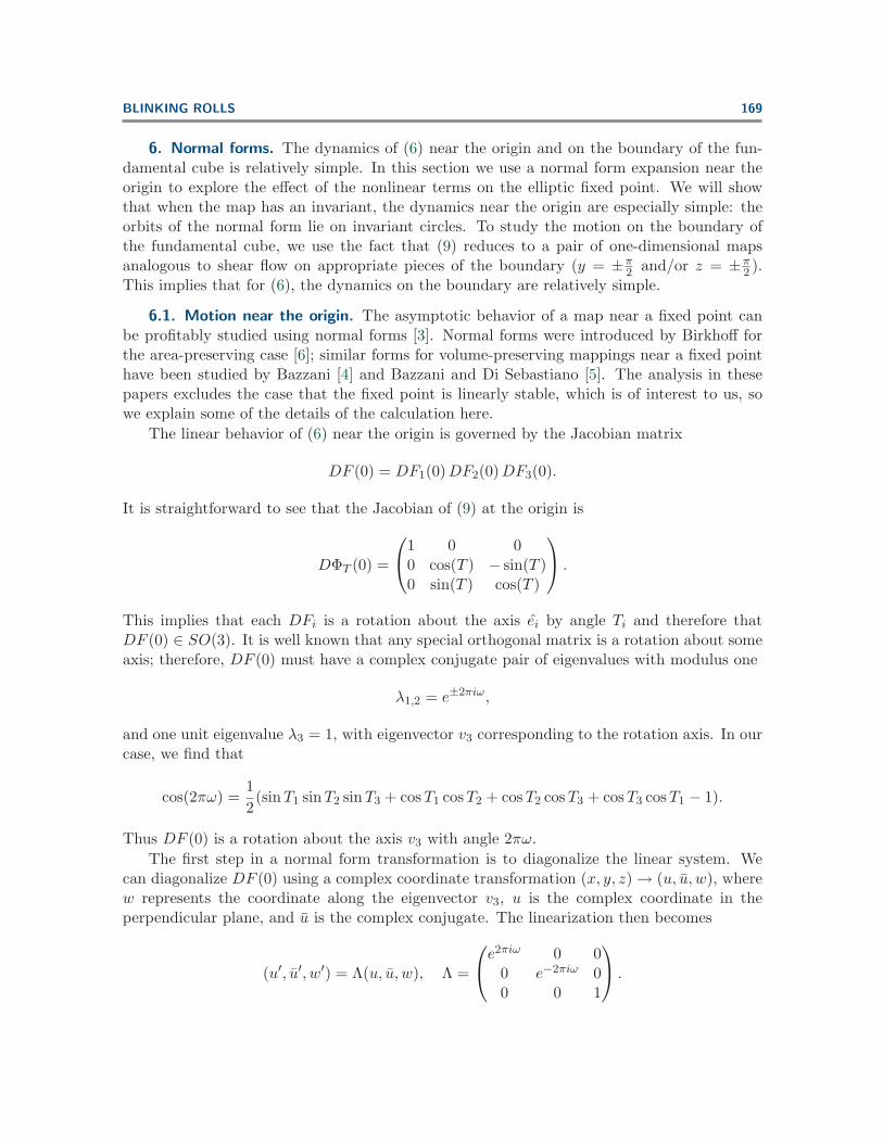
6. Normal forms. The dynamics of (6) near the origin and on the boundary of the fun-damental cube is relatively simple. In this section we use a normal form expansion near theorigin to explore the effect of the nonlinear terms on the elliptic fixed point. We will showthat when the map has an invariant, the dynamics near the origin are especially simple: theorbits of the normal form lie on invariant circles. To study the motion on the boundary ofthe fundamental cube, we use the fact that (9) reduces to a pair of one-dimensional mapsanalogous to shear flow on appropriate pieces of the boundary (y = ±π

2 and/or z = ±π2 ).

This implies that for (6), the dynamics on the boundary are relatively simple.

6.1. Motion near the origin. The asymptotic behavior of a map near a fixed point canbe profitably studied using normal forms [3]. Normal forms were introduced by Birkhoff forthe area-preserving case [6]; similar forms for volume-preserving mappings near a fixed pointhave been studied by Bazzani [4] and Bazzani and Di Sebastiano [5]. The analysis in thesepapers excludes the case that the fixed point is linearly stable, which is of interest to us, sowe explain some of the details of the calculation here.

The linear behavior of (6) near the origin is governed by the Jacobian matrix

DF (0) = DF1(0)DF2(0)DF3(0).

It is straightforward to see that the Jacobian of (9) at the origin is

DΦT (0) =

⎛⎝1 0 0

0 cos(T ) − sin(T )0 sin(T ) cos(T )

⎞⎠ .

This implies that each DFi is a rotation about the axis ei by angle Ti and therefore thatDF (0) ∈ SO(3). It is well known that any special orthogonal matrix is a rotation about someaxis; therefore, DF (0) must have a complex conjugate pair of eigenvalues with modulus one

λ1,2 = e±2πiω,

and one unit eigenvalue λ3 = 1, with eigenvector v3 corresponding to the rotation axis. In ourcase, we find that

cos(2πω) =1

2(sinT1 sinT2 sinT3 + cosT1 cosT2 + cosT2 cosT3 + cosT3 cosT1 − 1).

Thus DF (0) is a rotation about the axis v3 with angle 2πω.

The first step in a normal form transformation is to diagonalize the linear system. Wecan diagonalize DF (0) using a complex coordinate transformation (x, y, z) → (u, u, w), wherew represents the coordinate along the eigenvector v3, u is the complex coordinate in theperpendicular plane, and u is the complex conjugate. The linearization then becomes

(u′, u′, w′) = Λ(u, u, w), Λ =

⎛⎝e2πiω 0 0

0 e−2πiω 00 0 1

⎞⎠ .

170 P. MULLOWNEY, K. JULIEN, AND J. D. MEISS

We denote the map in the new coordinates u = (u, u, w) by F , so that DF(0) = Λ. ExpandF in a power series expansion of the form

F(u) = Λ(u + F (k)(u) + F (k+1)(u) + · · · ),

where F (k) is a term that is homogeneous of degree k > 1 in the variables u, i.e.,

F (k) =∑

m+n+p=k

am,n,pum unwp ,(18)

with m,n, p ∈ Z+, and complex coefficients am,n,p. Since the original map is real, u is thecomplex conjugate of u, and thus am,n,p = an,m.p.

The normal form for F is a “simpler” map G that is conjugate to F ,

G(h(u)) = h(F(u)),(19)

by a near identity transformation h. As usual we expand the conjugacy h and the new mapin power series and at each order use h to remove as many terms in G as possible. At orderk all terms in F (k) can be removed except those that are “resonant,” i.e., those terms in theqth component of (18) for which the integers satisfy

λm1 λn

2λp3 = e2πi(m−n)ω = λq.(20)

For each ω, we denote the solutions of (20) by R, and the normal form becomes

G = Λ(u + F (k)R (u) + · · · ),

where F (k)R denotes those terms in (18) for which m,n, p are in R.

When ω is irrational, (20) shows that resonances occur when

m = n + 1 for q = 1,m = n− 1 for q = 2,m = n for q = 3.

Since we can eliminate the nonresonant terms to all orders, the normal form becomes

u′ = e2πiωu

⎛⎝1 +

∑n,p≥0

α2n,p|u|2nwp

⎞⎠ ,

w′ = w

⎛⎝1 +

∑n,p≥0

β2n,p−1|u|2nwp−1

⎞⎠ ,(21)

where βn,p is real and α0,0 = β0,0 = 0, since the corrections must be nonlinear. As is truefor general normal form theory, (21) commutes with the group generated by Λ [14]; since weassumed ω is irrational, it commutes with arbitrary rotations about the w-axis. Note that theseries (21) is not guaranteed to converge, even in some neighborhood of the origin, and thusmust be viewed only in an asymptotic sense.

BLINKING ROLLS 171

As demonstrated in section 5, the map (6) has reflection symmetry through the origin. Inthis case, the normal form will exhibit the same symmetry, and therefore all even order termsdrop out of the expansion so that

α2n,2p+1 = β2n,2p+1 = 0.

In addition, if F is volume-preserving, then we can choose h so that it also preserves volume,and therefore the normal form will as well:

du′ ∧ du′ ∧ dw′ = du ∧ du ∧ dw.

This places restrictions on the coefficients of (21). To cubic order, we find

β2,0 = −4Re(α2,0), β0,2 = −2

3Re(α0,2).(22)

Now, we can analyze basic phenomena of the normal form. Letting u = ρe2πiθ, we canrewrite (21) to obtain the real map

ρ′ = ρ

(1 − 1

4β2,0ρ

2 − 3

2β0,2w

2 + O(3)

),

θ′ = θ + ω + Im(α2,0)ρ2 + Im(α0,2)w

2 + O(3),

w′ = w(1 + β2,0ρ2 + β0,2w

2 + O(3)).

Thus the origin is a nonhyperbolic fixed point. To all orders, the w-axis (ρ = 0) and theequatorial plane w = 0 are invariant. The plane w = 0 is locally an (un)stable manifold of theorigin when β2,0 > 0 (< 0), and the w-axis is locally (un)stable when β0,2 < 0 (> 0). There

are additional unstable manifolds along the lines ρ = sw when s2 = −2β0,2

β2,0> 0, and these are

(un)stable manifolds when β0,2 > 0(< 0). An example is shown in Figure 5.

ρ

w

θ

Figure 5. Dynamics of the normal form in the (ρ,w)-plane for β2,0 > 0 and β0,2 < 0.

Note that when there is an invariant whose surfaces are topological spheres about theorigin (as is the case for (6)), none of the invariant axes can be attracting or repelling. Thusthe only normal form that corresponds to this case is one in which every resonant coefficienthas real part zero. Thus the normal form for (6) with irrational ω fixes ρ and w, and everyorbit near the origin lies on an invariant circle. As we will see, this corresponds well with thenumerical observations of the dynamics of (6) in section 7.

172 P. MULLOWNEY, K. JULIEN, AND J. D. MEISS

6.2. Motion on the boundary cube. The single roll flow (9) preserves the boundaries ofthe fundamental cube; the surfaces where x, y, or z are ±π

2 . Recall from section 2 that theline (y, z) = (π2 ,

π2 ) and its translations by (mπ, nπ) consist of saddle equilibria of ΦT . The

four faces corresponding to the set {(y, z) : |y| = π2 or |z| = π

2 } correspond to their stable andunstable manifolds.

On these faces, the velocity field (3) has only one component, and its flow simplifies sincethere the modulus k → 1, and sn(T, 1) = tanh(T ), and cn(T, 1) = dn(T, 1) = sech(T ). In thiscase (9) becomes

ΦT (x, y, z) =

⎧⎪⎪⎨⎪⎪⎩

(x, y, sin−1

(cosh(T ) sin(z)±sinh(T )cosh(T )±sin(z) sinh(T )

))if y = ±π

2 ,

(x, sin−1

(cosh(T ) sin(y)∓sinh(T )cosh(T )∓sin(y) sinh(T )

), z)

if z = ±π2 .

(23)

This formula for T = T1 gives the boundary map corresponding to F1; we denote it as B1.The maps B2 and B3 are obtained from (23) by permuting the variables appropriately.

It is convenient to use a spherical projection to display the dynamics of the system.Letting (θ, η) denote the longitude and colatitude, respectively, we can project the cube ontothe sphere. Then the dynamics can be displayed on the rectangle −π < θ ≤ π, 0 ≤ η ≤ π. Forexample, in Figure 6 we show F1 and F3 in this projection. In this figure, the twelve edges ofthe cube project to the red curves. The faces x = ±π

2 are pierced in the center by the points(θ, η) = (0, π2 ) and (θ, η) = (π, π2 ), respectively. The faces defined by z = ±π

2 correspond tothose with η near 0 and π. The remaining panels define y = ±π

2 .

η

θ

0

1

2

3

-3 -1 1 3

x = π/2

y=π/

2

y =

–π/

2

x =– π/2

z = π/2

z =– π/2

η

θ

0

1

2

3

-3 -1 1 3

Figure 6. Maps on the boundary cube projected onto the spherical angles (θ, η). Invariant curves of F1 areshown in the left panel and those of F3 are shown in the right. Note that the two figures are equivalent undera positive rotation by π

2about the y-axis.

Now consider the two-roll composition

F1 ◦ F3.

Since the cube is an invariant surface for each map, it is still invariant. The eight vertices,v±±± = (±π/2,±π/2,±π/2), are saddle fixed-points. These points are represented by the

BLINKING ROLLS 173

intersections of the red curves in Figure 6. The edges of the cube now comprise parts of thestable or unstable manifolds of the saddle fixed-points.

On the two faces defined by y = ±π2 , the boundary behavior is given by B1 ◦B3 because

both of the moduli of the corresponding flows are one. Figure 6 shows simple dynamics onthis face corresponding to shear flows. The face y = π

2 is a branch of the stable manifold ofthe saddle v−++ (shown as a blue dot in Figure 6). Similarly, the boundary face y = −π

2is a branch of the stable manifold of v+−−. The Jacobian at the vertices is easily evaluatedby linearizing the flow at a saddle equilibrium to obtain DF1 = diag(1, es1T1 , e−s1T1), wheres1 = sgn(yz), and DF3 = diag(es3T3 , e−s3T3 , 1), where s3 = sgn(xy). Thus at the vertex v−++

DF1 ◦DF3 = diag(e−T3 , eT1+T3 , e−T1).(24)

On the four remaining faces, the dynamics is determined by either F1 ◦B3 or B1 ◦F3, andeven these simplified maps can have complicated behavior. Here we will discuss the existenceof fixed points. For example consider F1 ◦B3 on the face x = π/2. In the simplest case, whenT3 = 0, the dynamics is simply the sheared rotation defined by the single roll. The rotationnumber of F1 is

ω =T1

4K(k),

where K is the complete elliptic integral, and k is the modulus (8). Since K(0) = π2 , ω starts

at T12π at (π2 , 0, 0) and decreases to zero at the edges; therefore, there will be fixed points at

the center of the face and on any streamline for which ω is an integer. If we restrict ourattention to 0 < T1 < 2π, there is exactly one elliptic fixed point on the face—the point(π2 , 0, 0). Moreover, the implicit function theorem implies that this fixed point persists for T3

nonzero, since the elliptic fixed points have eigenvalues not equal to 1.Because B3 is applied before F1 and we are considering only rolls with positive rotation,

all fixed points reside on the y < 0 half of the face x = π2 . Since the streamlines of F1 are

symmetric about the plane y = 0, and B3 changes y only, any fixed point must occur on a liney = −c such that B3(−c, z) = (c, z), and correspondingly, we must have F1(c, z) = (−c, z).The points (±c, z) reside on the same streamline of F1, and therefore there must be a T1 suchthat F1(c, z) = (−c, z) (up to 4K periodicity) because the curves are continuous, closed loops.

Indeed, for large enough values of T1 there can be multiple fixed points on this face. Tosee this, consider the vertical line segments l± = {(y = ±c, z)}; see Figure 7. For each c, thereexists a T3 such that B3(l−) = l+. The image of l+ under F1 can be quite complex. As shownin the figure, if T1 < T3, F1(l+) does not intersect l−, and there are no fixed points on theface. For T1 = T3 , F1(l+) (the red curve) intersects l− at z = π

2 . When T1 is slightly greaterthan T3, we have at most one fixed point because there is only one intersection; however, ifT1 >> T3 (the cyan curve), there can be many fixed points. If there is one intersection, thenthis point is actually a fixed point, as symmetry implies that F1(c, z) = (−c, z). However, ifF1(l+) intersects l− in several places, not all intersections need have the same z coordinateafter iteration. When there exist more than three such intersections, then some of them canbe candidates for additional fixed points.

One can understand fixed points on the other faces by a similar argument.

174 P. MULLOWNEY, K. JULIEN, AND J. D. MEISS

-1 0 1

-1

0

1

T1

<T3

T1 =T3

T1 >T3 T1 >T3>

l+ l-

Figure 7. Fixed points of F1 ◦ B3 at x = π2. Here l+ = B3(l−) and the colored curves are images of l+

under F1.

7. Numerical explorations. In this section we will explore some of the dynamics (6). Forsimplicity, we set T2 = 0 so that the second roll is not active, giving the system

F = F1 ◦ F3.(25)

As we showed in section 5, it is sufficient to consider to T1 > T3 > 0.First we discuss the techniques that we will use to visualize the orbits of (25). We

take advantage of the fact that orbits are constrained to surfaces of constant J(x, y, z) =cos(x) cos(y) cos(z), and that for each 0 < J ≤ 1 these surfaces are convex, topologicalspheres; recall Figure 3. Therefore, as we did in section 6.2 for the maps on the boundary, wecan use spherical coordinates to obtain a two-dimensional projection of the dynamics. Letting(θ, η) be the spherical angles, any point (x, y, z) corresponds to a point (J, θ, η), and since Jis invariant, we can view the dynamics in the angle plane. The coordinate transformation isthus

(J, θ, η) = V (x, y, z) =

(cos(x) cos(y) cos(z), tan−1

(yx

), tan−1

(√x2 + y2

z

)),(26)

which has the Jacobian

det(DV ) = Jx tanx + y tan y + z tan z√

x2 + y2(x2 + y2 + z2).(27)

To visualize the dynamics on the (θ, η)-plane for a given invariant value, we will iterate a gridof initial conditions. For each (θ, η), we first determine the radius, r, using the Newton methodon J(r sin η cos θ, r sin η sin θ, r cos η), and then transform to Cartesian coordinates to obtainthe initial point for (25). For subsequent iterates, we can simply project out the spherical

BLINKING ROLLS 175

radius and plot (θ, η) along the orbit. To view the dynamics in the entire cube, we choose agrid in J (from 1 to 0) and concatenate the figures to create the animations 60672 01.avi and60672 02.avi. The animations reveal a system rich in complex, chaotic behavior.

Recall that when a map has an invariant, fixed points generically come in one-parameterfamilies labeled by the invariant value [20]. Suppose that O = {xt, t = 0, . . . , n − 1} is aperiodic orbit of period n. Differentiating the equation J(Fn(x)) = J(x) at the point x0 gives

(DFn(x0))T · ∇J(x0) = ∇J(x0).(28)

Thus when ∇J(x0) �= 0 (as is true on all invariant surfaces except the origin and the funda-mental cube), this vector is a left eigenvector of the Jacobian with unit multiplier. Since Fis volume-preserving, this implies that the multipliers of O are (1, λ, 1

λ). When λ �= 1, theimplicit function theorem can be used to show there is a curve of fixed points of Fn parame-terized by J through x0. When λ �= ±1, the periodic orbit is elliptic on the invariant surface ifλ is on the unit circle and hyperbolic when λ is real. The orbit generically undergoes q-tuplingbifurcations when λ passes through the value e2πiω with ω = p/q rational. These bifurcationscorrespond to the creation of new periodic orbits of period nq; these new orbits are also foundin one-parameter families parameterized by J .

To compute some of the low period orbits we use Broyden’s method [16]. For the fixedpoints, we allowed the initial guess for Broyden’s method to range over the entire invariantsurface, so that we had a good chance of finding all of them. However, to limit the complexityof the figures, we decided only to search for periodic points born at the q-tupling bifurcationsof the fixed points. An analytic expression for the Jacobian can be computed to determinethe stability of the periodic points.

The analysis of fixed and periodic points gives us the ability to understand the fine struc-ture of the system. It also illuminates any barriers to global transport on each invariant. Forinstance, the existence of large islands surrounding stable periodic points inhibits the trans-port of passive scalars. On the other hand, the existence of hyperbolic periodic points shouldaid transport due to the likelihood of homoclinic and heteroclinic tangles in their manifolds.

One measure of the degree of chaos in a system are its Lyapunov exponents. Since F isvolume-preserving, the sum of its three exponents must be zero, and because the orbits arerestricted to two-dimensional surfaces, one of the exponents must be exactly equal to zero.This implies that the remaining two exponents are equal in magnitude and opposite in sign.We use the iterative QR method to compute the exponents [21]. Along an orbit O, define

Q(n+1) R(n+1) = DF (xn)Q(n) R(n),

where Q(0) = R(0) = id. As usual Q is orthogonal and R is upper triangular. To computethe exponents, we require that Rii > 0; it is not hard to show that one can modify the QRmethod so that this is the case. Moreover, since F is orientation-preserving and det(R) > 0,then Q ∈ SO(3). Thus we can represent Q with three angles, θi (for example, Euler angles orrotations about three orthogonal axes). Since

R(n+1) (R(n))−1 = (Q(n+1))T DF (xn)Q(n)

176 P. MULLOWNEY, K. JULIEN, AND J. D. MEISS

is upper triangular, this requirement can be manipulated to provide a formula for updatingthe angles θi iteratively. After n steps, the ith Lyapunov exponent is approximately

λ(n)i =

lnR(n)ii

n.

They can be computed iteratively using

λ(n)i =

1

n

((n− 1)λ

(n−1)i + ln((Q(n))T DF (xn)Q(n−1))ii

).

We compute the exponents on a (θ, η) grid of initial conditions on each invariant surface.In order to resolve islands from the chaotic sea, a very fine grid is used and a large number ofiterations are performed to get reasonable accuracy in the exponent. For all animations, Fig-ures 11, 12, 15, and 16, 15000 iterations were performed on an 81×51 grid of initial conditionson each invariant surface.2 We measure accuracy by averaging the standard deviation, 〈σ〉,of the final 1000 iterates over a given invariant via (29). As expected the accuracy dependsstrongly on the behavior in the phase plane. For the example given in section 7.1, we find〈σ〉 = .0001 when J = .1 and 〈σ〉 = .0115 when J = .8. Between these values, an increasingtrend is noted as the behavior evolves from regular to increasingly chaotic. For Figures 14and 17, 15000 iterations were also performed on slightly smaller grids of size 81 × 41.

As an average measure of chaos on the invariant surface we compute the surface averageof the positive Lyapunov exponent. The average of any function on a surface is approximatedby

〈f〉 =1

A

nθ,nη∑i,j

f(xij)|∇J(xij)|∆θ∆η

|det(DV (xij)|.(29)

Here |∇J |/|det(DV )| is the surface area element with the Jacobian (27), A, the surface area,is determined so that 〈1〉 = 1, and xij is the ijth point on the surface grid with spacing ∆θand ∆η.

We expect the Lyapunov exponents will be very small near the origin, since the normalform analysis in section 6.1 indicates that orbits near the origin lie on invariant circles. Simi-larly the Lyapunov exponents near the boundary cube will tend toward those on the boundaryfaces. Recall that two of the boundary faces, y = ±π

2 , correspond to branches of the stablemanifold of vertices. From (24), the Lyapunov exponents on these faces are (−T3,−T1). How-ever, on the four remaining faces, the dynamics are quite complex. We will see that the effectof the uniform faces is to decrease the Lyapunov exponents near the boundary.

7.1. Example 1: T1 + T3 = 12. We begin by exploring some of the dynamics of (25)for the case T1 = 7, T3 = 5. Recall that near the origin, the map is approximately a rotationabout the axis v3, where v3 is the eigenvector of DF (0) with eigenvalue one. In Figure 8 weshow a projection of the dynamics onto the (θ, η)-plane for J near one; since J = 1 at theorigin, the portrait shown in the figure corresponds to a small sphere near the origin. Most

2 For the animations, Figures 12 and 16, 399 invariant values were used. The generation of the Lyapunovdata took approximately two weeks to run on a Pentium 4 processor.

BLINKING ROLLS 177

of the orbits lie on invariant circles, as suggested by the normal form analysis in section 6.1.The apparent change in topology of the circles in the figure is due only to nonalignment ofthe spherical projection with the rotation axis. Note that the reflection symmetry throughthe origin implies that the northern and southern hemispheres have conjugate dynamics.

Figure 8. Projection of the dynamics of (25) onto the (θ, η)-plane for T1 = 7, T3 = 5, on the invariantsurface J = 0.973962.

There is a curve of fixed points tangent to the v3-axis at the origin; this gives rise to a pairof fixed points on each invariant surface, and for these parameter values there are no otherfixed points. We focus on the fixed point in the northern hemisphere—by symmetry the otherfixed point has the same behavior. In Figure 9, we plot the multipliers (1, λ, λ−1) of this fixedpoint as a function of J . Note that J = 1 at the top of the figure, corresponding to the originin phase space, and J decreases to 0 at the base of the figure, corresponding to the boundingcube. Several q-tupling bifurcations are labeled in the figure.

The phase space near several of these bifurcations is shown in Figure 10. In this figurethe four panels on the left show the tripling bifurcation near J ≈ .61 (corresponding to thesquares in Figure 9). As is usual for area-preserving maps, there is a saddle-center bifurcationcreating a pair of period-three orbits before the rotation number of the fixed point reaches13 . In the interval J ∼= .628 to J ∼= .623, there is a bubble creating and destroying two newunstable period-three orbits in a pair of subcritical pitchfork bifurcations. As the rotationnumber approaches 1

3 , the saddle then collides with the fixed point at the tripling and laterreappears on the opposite side. The bifurcation sequence is completed as the saddle-centerpair experiences a subcritical saddle-center bifurcation thus annihilating the pair just afterJ = .5508278.

The four panels on the right show a sequence of period-two bifurcations near J ≈ .45(corresponding to the small bubble of instability in Figure 9). The first doubling is supercrit-ical, resulting in the creation of a stable period-two orbit (the fixed point becomes unstable).Subsequently at J ≈ .448465, the unstable fixed point undergoes a subcritical doubling event,

178 P. MULLOWNEY, K. JULIEN, AND J. D. MEISS

Figure 9. Multipliers of the fixed point of (25) as a function of J for T1 = 7 and T3 = 5. Doubling, tripling,and quadrupling bifurcations are noted.

thus spawning an unstable period-two orbit. At J ≈ .448222, the unstable period-two orbitcreated from the previous split undergoes a pitchfork bifurcation, thus creating a pair of un-stable period-two orbits and a stable period-two orbit. When the sequence finishes, we havea stable fixed point, two stable period-two orbits, and two unstable period-two orbits. Thereis a final supercritical doubling of the fixed point near J = 0.27, and for all smaller values ofJ , the fixed points are unstable.

In the QuickTime file 60672 01.avi, we present an animation of the dynamics and maximalLyapunov exponent for these parameter values. The movie consists of 399 frames starting atJ = .999 and decreasing to J = 0.002504. For the dynamics panel, each initial condition on thegrid of 14×14 points is iterated 1000 times.3 Also shown in the movie are panels that displaythe position of the fixed point in space, and its multipliers in the complex plane. A snapshot ofthe animation is shown in Figure 11. The computations show a clear correspondence betweenthe existence of island structures and small Lyapunov exponents. Outside of the islands,the Lyapunov exponent is nearly constant; however, there are several intervals of J whereinvariant circles far from the fixed points reappear (they are mostly destroyed for J < 0.75),and this causes a local reduction in the chaos. In general, as J decreases, the dynamicsbecome more chaotic; though as J nears zero the influence of the boundary dynamics appearsin the animation by a concentration of chaotic motion near the edges of the cube and thereappearance of islands that correspond to stable fixed points on the boundary.

In Figure 12 we show the scaled surface average of the largest Lyapunov exponent, 〈λ〉T

(where T = T1 +T3), as a function of J using (29). Prominent bifurcations and characteristics

3 Note the movie does not quite start and end at J = 1 and 0. J = 1 corresponds to the lone fixed pointat the origin; thus we omitted this frame. For J = 0, the Lyapunov code exhibited extreme sensitivity whichcould not be resolved easily. In addition, close to bifurcation points, stability classification of fixed points isalso numerically sensitive.

BLINKING ROLLS 179

Figure 10. Tripling and doubling bifurcations of a fixed point for T1 = 7, T3 = 5. The fixed point isshown as the blue circle, the green diamond and purple square correspond to stable and unstable period-threeorbits, and the red diamond and yellow square are stable and unstable period-two orbits. The four panels atthe left correspond to the following: (a) J = 0.625940, just after the first subcritical pitchfork bifurcation. (Forresolution in our figures, the full phase plane is not shown. Hence one stable period-three point is omitted. Twoadditional unstable period-three points are shown (bottom left, bottom right) which are part of another unstableperiod-three orbit.) (b) J = 0.618429, just before tripling bifurcation. (c) J = 0.600902. (d) J = 0.578368 afterthe tripling. The right panels correspond to (e) J = 0.465699 and (f) J = 0.450677, just before and after thefirst supercritical doubling, and (c) J = 0.445669 and (d) J = 0.428143, after the second subcritical doublingand pitchfork bifurcations.

Figure 11. Phase plane and the Lyapunov exponent for J = 0.262895. Points in the phase plane (upperpanel) correspond to periodic orbits; colors are the same as in Figure 10. The bottom panel shows the largestLyapunov exponent for a grid of initial conditions. Clicking on the above image displays the associated movie(60672 01.avi).

180 P. MULLOWNEY, K. JULIEN, AND J. D. MEISS

of the phase portrait are indicated on the figure. The scaled average Lyapunov exponentremains nearly zero as J decreases from 1, until near J = 0.8, when 〈λ〉

T suddenly begins toincrease. This suggests that the asymptotic validity of the normal form breaks down nearthis point and corresponds with the appearance of small zones of chaotic behavior. At thequadrupling and tripling bifurcations, 〈λ〉

T reaches local maxima, and two local minima are

associated with prominent period-two islands. The global maximum of 〈λ〉T occurs just inside

the boundary, after which a steep decrease occurs. As we saw in section 6.2, this is to beexpected because the Lyapunov exponents are negative on two of the six boundary faces.

T<λ>

0.04

0.03

0.02

0.01

J0.20.40.60.8

tripling

quadrupling

period 2 islands

doubling

few islands

islands near poles

Figure 12. Average scaled maximal Lyapunov exponent for T1 = 7, T3 = 5.

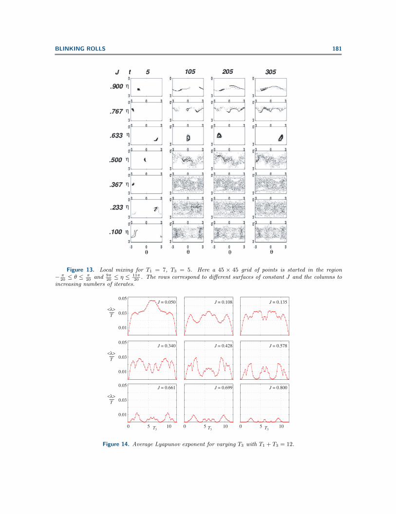
Though three-dimensional mixing is forbidden by the existence of the invariant, mixingdoes occur on the invariant surfaces. To visualize this, we start a group of points in a smallregion (see Figure 13) and view them at successive times. Results of these computationsreinforce the conclusion that limited transport occurs near the origin but that as J decreases,mixing occurs on increasing scales and more rapidly. This mixing, however, is not complete,as islands can be seen in the panels even with the smallest values of J .

To explore the dependence of the Lyapunov exponents on the choice of parameters, wenow fix T1 + T3 = 12 and vary the times in Figure 14. For each panel in the figure, 〈λ〉

T isplotted as a function of T3 for a fixed J . Note that each figure is symmetric about the pointT1 = T3, as predicted by the symmetry analysis in section 5. This figure shows that there isno choice of T3 such that 〈λ〉

T is maximized on every invariant surface; however, there are large

values of 〈λ〉T for most J when T3 ≈ 2 or 10. This case might be expected to have the largest

two-dimensional mixing on the surfaces of constant J .

The dynamics on the cubical boundary for this case are relatively uninteresting. Theadvection is so strong that the vast majority of iterates get pushed to the vertices or edges

BLINKING ROLLS 181

Figure 13. Local mixing for T1 = 7, T3 = 5. Here a 45 × 45 grid of points is started in the region− π

20≤ θ ≤ π

20and 9π

20≤ η ≤ 11π

20. The rows correspond to different surfaces of constant J and the columns to

increasing numbers of iterates.

0.01

0.03

0.05

0 5 10 0 5 10 0 5 10T3 T3 T3

J = 0.050 J = 0.108 J = 0.135

J = 0.340 J = 0.428 J = 0.578

J = 0.661 J = 0.699 J = 0.800

T<λ>

0.01

0.03

0.05

T<λ>

0.01

0.03

0.05

T<λ>

Figure 14. Average Lyapunov exponent for varying T3 with T1 + T3 = 12.

182 P. MULLOWNEY, K. JULIEN, AND J. D. MEISS

almost immediately.

7.2. Example 2: T1 + T3 = 6. In this section we fix the total time to T1 + T3 = 6, halfof the previous value. We will first consider the case T1 = 3.5 and T3 = 2.5 and see that thedynamics on the boundary has an influence that extends far into the interior of the cube.

We observe that for this case, as in section 7.1, there is a single curve of fixed pointsthat emanates from the origin. The fixed points also have a bubble of instability that beginswith a supercritical doubling near J ≈ 0.92. Two new pairs of period-two orbits are born insaddle-center bifurcations near the poles when J ≈ 0.8, and the new stable period-two orbitscollide with the fixed points in a subcritical doubling at J ≈ 0.77, completing the bubble.Unlike the previous case, the fixed points do not undergo another doubling bifurcation afterthey regain stability as J continues to decrease; instead they remain stable (apart from amomentary instability at several tripling bifurcations) to J = 0. These fixed points continueto those on the boundary faces x = ±π

2 .In Figure 15 we show two panels from the animation 60672 02.avi for this case. In the

left panel, where J = 0.282925, there are large period-three islands surrounding the fixedpoint—these were born in a saddle-center bifurcation at J ≈ 0.306. Islands from an earlierfive-tupling bifurcation are also prominent (one of these islands encloses the pole and is thushard to see in the projection). A band of regular behavior corresponding to invariant circlesseparates the surface into two invariant hemispheres; these have conjugate dynamics underthe reflection symmetry R in (15).

The right panel of Figure 15 shows the case J = 0.030045, close to the bounding cube.In this case there is an even larger band of meandering, invariant circles and a correspondingregion of the small Lyapunov exponents. The boundary dynamics (recall Figure 6) stronglyinfluences the dynamics on this surface. In the regions that correspond to the faces y = ±π

2 ,the dominant motion sweeps the trajectories across the face and helps give rise to the invariantcircles. Near the faces x = ±π

2 , the dynamics is predominantly chaotic, with the exception ofsmall elliptic islands around the sole fixed point on each face.

In Figure 16 we show the average Lyapunov exponent as a function of J . As in Figure12, 〈λ〉

T ≈ 0 for an initial interval near the origin; however, now 〈λ〉T increases more or less

monotonically, until J ≈ 0.22, when it plunges rapidly to a local a minima at J ≈ 0.14. Thisplunge occurs when the fixed points have multipliers that hover near the tripling point andseems to be associated with the creation of many modest size elliptic regions in the phasespace. Note that the overall magnitude of 〈λ〉

T is similar in this case to the previous one upuntil J ≈ .22.

Finally, we show 〈λ〉 as a function of T3 for T1 + T3 = 6 in Figure 17. Once again, there

seems to be no consistent choice of T1 and T3 such that 〈λ〉T is maximized over every invariant.

It is interesting to note, however, that near the origin, 〈λ〉T is maximized for equal times, in

contrast with the results in Figure 14. However, as before, the largest Lyapunov exponentson most surfaces seem to occur when the time parameters substantially differ, in this case forT3 = 1.5 or 4.5.

8. Conclusions. In 1984, Aref outlined a general, mathematically tractable stirring proto-col for passive tracers chaotically advected by point vortices with specified location, strength,and lifetime. We have presented a simple, three-dimensional, incompressible flow analogous

BLINKING ROLLS 183

Figure 15. Dynamics for T1 = 3.5, T3 = 2.5. The left panels correspond to J = 0.282925 and the right toJ = 0.030045. Clicking on the above images displays the associated movie (60672 02.avi).

0.01

0.02

J0.20.40.60.8

subcritical doubling

period 2saddle-center

doubling

subcritical tripling

T<λ>

0

Figure 16. Surface average of the maximal Lyapunov exponent as a function of J for T1 = 3.5, T3 = 2.5.

to Aref’s two-dimensional blinking vortex model. In its most general form our model consistsof a superposition of nonautonomous two-dimensional roll arrays. It simplifies considerably ifthe rolls act sequentially and are turned on and off instantaneously; for in this case, each two-dimensional flow lies on streamlines of the corresponding stream function. We have studied thecase of orthogonal roll arrays with identical aspect ratio in detail, where the two-dimensionalflow can be obtained analytically in terms of elliptic functions.

184 P. MULLOWNEY, K. JULIEN, AND J. D. MEISS

0.01

0 2 4 6T3

0 2 4 6T3

0 2 4 6T3

J = 0.030 J = 0.060 J = 0.140

J = 0.160 J = 0.220 J = 0.265

J = 0.320 J = 0.600 J = 0.806

0.03

0.01

0.03

0.01

0.03

T<λ>

T<λ>

T<λ>

Figure 17. Average Lyapunov exponent vs time, fixed invariants.

For this case there is an invariant J , (14), so that the motion is confined to topologicalspheres. As shown in section 4, the invariant is a product of the orthogonality of the rollsand exists under any stirring protocol. Nevertheless, the dynamics on each two-dimensionalsurface can exhibit all of the complexity of area-preserving mappings. We have shown that thedynamics near the intersection of the centers of the rolls lies on families of invariant circlesand can be described by an asymptotic normal form. The corresponding phase portraitsshow no chaos in this regime. The motion is constrained by the outermost boundary, whichfor our system is an invariant cube. Each face of the cube is invariant, and several of thefaces have simpler dynamics corresponding to laminar shear and/or laminar shear followed byrotation. The onset of chaos occurs suddenly some distance from the origin, and, as measuredby Lyapunov exponents, exhibits irregular growth as we continue to move away from theorigin that is associated with bifurcations of fixed points and low period orbits.

In order to achieve true three-dimensional mixing in systems composed of roll arrays, theinvariant must be broken. In [17], roll arrays of identical aspect ratio and axes given by e2

and e3 were positioned such that their respective intersections with the e1-axis were 90◦ out ofphase. Their investigations showed local and global three-dimensional mixing. Other possibleconstructions that may achieve three-dimensional mixing include (non)orthogonal roll arrayswith identical/different aspect ratios. In the case of nearly orthogonal alternating roll arrayswith identical aspect ratio, our preliminary investigations have shown that the invariant is infact destroyed by this kind of perturbation. Initial studies indicate that the mixing near theintersection of roll axes is strongly influenced by the former invariant surfaces. This case alsoallows for transport between adjacent rolls. This case is unusual in a perturbation sense, sincethe unperturbed flow is chaotic itself. In the idealized limit where we consider infinite rollarrays, studies of transport throughout the domain can be understood under the framework of

BLINKING ROLLS 185

anomalous diffusion theory [24, 27, 26, 25]. In a construction analogous to the Kuppers–Lortzphenomenon, roll arrays rotating by 60◦ also display three-dimensional mixing. We will reporton these topics in a future paper.

Acknowledgments. We would like to thank H. E. Lomelı and P. Boyland for helpfuldiscussions.

REFERENCES

[1] H. Aref, Stirring by chaotic advection, J. Fluid Mech., 143 (1984), pp. 1–21.[2] H. Aref, The development of chaotic advection, Phys. Fluids, 14 (2002), pp. 1315–1325.[3] D. Arrowsmith and C. Place, An Introduction to Dynamical Systems, Cambridge University Press,

Cambridge, UK, 1990.[4] A. Bazzani, Normal form theory for volume-preserving maps, Z. Angew. Math. Phys., 44 (1993), pp.

147–172.[5] A. Bazzani and A. Di Sebastiano, Perturbation theory for volume-preserving maps: Application to the

magnetic field lines in plasma physics., in Analysis and Modelling of Discrete Dynamical Systems,Adv. Discrete Math. Appl. 1, Gordon and Breach, Amsterdam, 1998, pp. 283–300.

[6] G. Birkhoff, Surface transformations and their dynamical applications, Acta Math., 43 (1920), pp.1–119.

[7] P. Boyland, personal communication, 2003.[8] M. Brown and K. Smith, Ocean stirring and chaotic low-order dynamics, Phys. Fluids, 3 (1991), pp.

1186–1192.[9] F. Busse and K. E. Heikes, Convection in a rotating layer—simple case of turbulence, Science, 208

(1980), pp. 173–175.[10] P. F. Byrd and M. D. Friedman, Handbook of Elliptic Integrals for Engineers and Physicists, Springer-

Verlag, New York, 1954.[11] J. Cartwright, M. Feingold, and O. Piro, Chaotic advection in three dimensional unsteady incom-

pressible laminar flow, J. Fluid Mech., 316 (1996), pp. 259–284.[12] J. H. E. Cartwright, M. O. Feingold, and O. Piro, Passive scalars and three-dimensional Liouvillian

maps, Phys. D, 76 (1994), pp. 22–33.[13] T. Dombre, U. Frisch, J. Greene, M. Henon, A. Mehr, and A. Soward, Chaotic streamlines in

the ABC flows, J. Fluid Mech., 167 (1986), pp. 353–391.[14] C. Elphick, E. Tirapegui, M. Brachet, P. Coullet, and G. Iooss, A simple global characterization

for normal forms of singular vector fields, Phys. D, 29 (1987), pp. 95–127.[15] M. Feingold, L. Kadanoff, and O. Piro, Passive scalars, three-dimensional volume-preserving maps,

and chaos, J. Statist. Phys., 50 (1988), pp. 529–565.[16] B. P. Flannery, W. H. Press, S. A. Teukolsky, and W. T. Vetterling, Numerical Recipes in C,

The Art of Scientific Computing, 2nd ed., Cambridge University Press, Cambridge, UK, 1992.[17] M. Fogleman, M. Fawcett, and T. Solomon, Lagrangian chaos and correlated Levy flights in a

non-Beltrami flow: Transient versus long-term transport, Phys. Rev. E (3), 63 (2001), pp. 1–4.[18] G. Fountain, F. Khakhar, and J. Ottino, Visualization of three-dimensional chaos, Science, 281

(1998), pp. 683–686.[19] G. O. Fountain, D. V. Khakhar, I. Mezic, and J. Ottino, Chaotic mixing in a bounded three-

dimensional flow, J. Fluid Mech., 417 (2000), pp. 265–301.[20] A. Gomez and J. Meiss, Volume-preserving maps with an invariant, Chaos, 12 (2002), pp. 289–299.[21] S. Habib, T. Janaki, G. Rangarajan, and R. D. Ryne, Computation of the Lyapunov spectrum for

continuous-time dynamical systems and discrete maps, Phys. Rev. E (3), 60 (1999), pp. 6614–6626.[22] Y. Hu, W. Pesch, G. Ahlers, and R. Ecke, Convection under rotation for Prandtl numbers near 1:

Kuppers-Lortz instability, Phys. Rev. E (3), 58 (1998), pp. 5821–5833.[23] C. Jones and S. Winkler, Invariant manifolds and Lagrangian dynamics in the ocean and atmosphere,

in Handbook of Dynamical Systems, Vol. 2, North–Holland, Amsterdam, 2002, pp. 55–92.

186 P. MULLOWNEY, K. JULIEN, AND J. D. MEISS

[24] J. Klafter, A. Blumen, and M. Shlesinger, Stochastic pathway to anomalous diffusion, Phys. Rev.A (3), 35 (1987), pp. 3081–3085.

[25] J. Klafter, M. Shlesinger, and G. Zumofen, Beyond Brownian motion, Physics Today, 49 (1996),pp. 33–39.

[26] J. Klafter, G. Zumofen, and M. Shlesinger, Anomalous diffusion and Levy statistics in intermittentchaotic systems, in Chaos: The Interplay between Stochastic and Deterministic Behavior, LectureNotes in Phys. 457, Springer-Verlag, Berlin, 1995, pp. 183–210.

[27] J. Klafter, G. Zumofen, M. Shlesinger, and A. Blumen, Scale invariance in anomalous diffusion,Philosophical Magazine B, 65 (1992), pp. 755–765.

[28] G. Kuppers and D. Lortz, Transition from laminar convection to thermal turbulence in a rotating fluidlayer, J. Fluid Mech., 35 (1969), pp. 609–620.

[29] H. Lomeli and J. Meiss, Quadratic volume-preserving maps, Nonlinearity, 11 (1998), pp. 557–574.[30] H. Lomeli and J. Meiss, Heteroclinic primary intersections and codimension one Melnikov method for

volume-preserving maps, Chaos, 10 (2000), pp. 109–121.[31] H. E. Lomeli and J. Meiss, Heteroclinic orbits between invariant circles in volume-preserving mappings,

Nonlinearity, 16 (2003), pp. 1573–1595.[32] C. Lopez, E. Hernandez-Garcia, O. Piro, A. Vulpiani, and E. Zambianchi, Population dynamics

advected by chaotic flows: A discrete-time map approach, Chaos, 11 (2001), pp. 397–403.[33] G. Metcalfe, T. Shinbrot, J. McCarthy, and J. M. Ottino, Avalanche mixing of granular solids,

Nature, 374 (1995), pp. 39–41.[34] E. Moses and V. Steinberg, Stationary convection in a binary mixture, Phys. Rev. A (3), 43 (1991),

pp. 707–722.[35] Z. Neufield, P. Haynes, and T. Tel, Chaotic mixing induced transitions in reaction-diffusion systems,

Chaos, 12 (2002), pp. 426–438.[36] J. Ottino, The Kinematics of Mixing: Stretching, Chaos, and Transport, Cambridge University Press,

Cambridge, UK, 1989.[37] O. Piro and M. Feingold, Diffusion in three-dimensional Liouvillian maps, Phys. Rev. Lett., 61 (1988),

pp. 1799–1802.[38] L. Rom-Kedar, V. Kadanoff, E. Ching, and C. Amick, The break-up of a heteroclinic connection in

a volume preserving mapping, Phys. D, 62 (1993), pp. 51–65.[39] I. Scheuring, G. Karolyi, Z. Toroczkai, T. Tel, and A. Pentek, Competing populations in flows

with chaotic mixing, Theoretical Populational Biology, 63 (2003), pp. 77–90.[40] T. Shinbrot, M. Alvarez, J. Zalc, and F. Muzzio, Attraction of minute particles to invariant regions

of volume preserving flows by transients, Phys. Rev. Lett., 86 (2001), pp. 1207–1210.[41] A. Stroock, S. Dertinger, A. Ajdari, I. Mezic, H. Stone, and G. Whitesides, Chaotic mixer for

microchannels, Science, 295 (2002), pp. 647–651.[42] R. Toral, M. San Miguel, and R. Gallego, Period stabilization in the Busse-Heikes model of the

Kuppers-Lortz instability, Phys. A, 280 (2000), pp. 315–336.[43] Y. Tu and M. Cross, Chaotic domain structure in rotating convection, Phys. Rev. Lett., 69 (1992), pp.

2515–2518.