Embed Size (px)
Citation preview
BlinkML: Efficient Maximum Likelihood Estimationwith Probabilistic Guarantees
Yongjoo Park, Jingyi Qing, Xiaoyang Shen, Barzan MozafariUniversity of Michigan, Ann Arbor
pyongjoo,jyqing,xyshen,[email protected]
ABSTRACT
The rising volume of datasets has made training machinelearning (ML) models a major computational cost in the en-terprise. Given the iterative nature of model and parametertuning, many analysts use a small sample of their entiredata during their initial stage of analysis to make quick deci-sions (e.g., what features or hyperparameters to use) and usethe entire dataset only in later stages (i.e., when they haveconverged to a specific model). This sampling, however, isperformed in an ad-hoc fashion. Most practitioners cannotprecisely capture the effect of sampling on the quality oftheir model, and eventually on their decision-making pro-cess during the tuning phase. Moreover, without systematicsupport for sampling operators, many optimizations andreuse opportunities are lost.In this paper, we introduce BlinkML, a system for fast,
quality-guaranteed ML training. BlinkML allows users tomake error-computation tradeoffs: instead of training amodelon their full data (i.e., full model), BlinkML can quickly trainan approximate model with quality guarantees using a sam-ple. The quality guarantees ensure that, with high probability,the approximate model makes the same predictions as thefull model. BlinkML currently supports any ML model thatrelies on maximum likelihood estimation (MLE), which in-cludes Generalized Linear Models (e.g., linear regression,logistic regression, max entropy classifier, Poisson regres-sion) as well as PPCA (Probabilistic Principal ComponentAnalysis). Our experiments show that BlinkML can speedup the training of large-scale ML tasks by 6.26×–629× whileguaranteeing the same predictions, with 95% probability, asthe full model.ACM Reference Format:
Yongjoo Park, Jingyi Qing, Xiaoyang Shen, Barzan Mozafari. 2019.BlinkML: Efficient Maximum Likelihood Estimation with Proba-bilistic Guarantees. In 2019 International Conference on Management
Permission to make digital or hard copies of all or part of this work for personal orclassroom use is granted without fee provided that copies are not made or distributedfor profit or commercial advantage and that copies bear this notice and the full cita-tion on the first page. Copyrights for components of this work owned by others thanthe author(s) must be honored. Abstracting with credit is permitted. To copy other-wise, or republish, to post on servers or to redistribute to lists, requires prior specificpermission and/or a fee. Request permissions from [email protected] ’19, June 30-July 5, 2019, Amsterdam, Netherlands
© 2019 Copyright held by the owner/author(s). Publication rights licensed to ACM.ACM ISBN 978-1-4503-5643-5/19/06. . . $15.00https://doi.org/10.1145/3299869.3300077
of Data (SIGMOD ’19), June 30-July 5, 2019, Amsterdam, Netherlands.
ACM, New York, NY, USA, Article 4, 18 pages. https://doi.org/10.1145/3299869.3300077
1 INTRODUCTION
While data management systems have been widely success-ful in supporting traditional OLAP-style analytics, they havenot been equally successful in attracting modern machinelearning (ML) workloads. To circumvent this, most analyticaldatabase vendors have added integration layers for popu-lar ML libraries in Python (e.g., Oracle’s cx_Oracle [4], SQLServer’s pymssql [9], and DB2’s ibm_db [10]) or R (e.g., Ora-cle’s RODM [11], SQL Server’s RevoScaleR [12], and DB2’sibmdbR [6]). These interfaces simply allowmachine learningalgorithms to run on the data in-situ.However, recent efforts have shown that data manage-
ment systems have much more to offer. For example, materi-alization and reuse opportunities [15, 16, 31, 93, 106], cost-based optimization of linear algebraic operators [24, 29, 48],array-based representations [59, 96], avoiding denormaliza-tion [64, 65, 89], lazy evaluation [109], declarative inter-faces [80, 95, 101], and query planning [63, 81, 94] are allreadily available (or at least familiar) database functional-ities that can deliver significant speedups for various MLworkloads.
One additional but key opportunity that has been largelyoverlooked is the sampling abstraction offered by nearly ev-ery database system. Sampling operators have been mostlyused for approximate query processing (AQP) [27, 32, 35,45, 54, 68, 73, 82, 84, 85]. However, applying the lessonslearned in the data management community regarding AQP,we could use a similar sampling abstraction to also speed upan important class of ML workloads.
Our Goal Given that (sub)sampling is already quite com-mon in early stages of ML workloads—such as feature selec-tion and hyper-parameter tuning—we propose a high-levelsystem abstraction for training ML models, with which an-alysts can explicitly request error-computation trade-offsfor several important classes of ML models. This involvessystematic support for (i) bounding the deviation of the ap-proximate model’s predictions from those of the full model
SIGMOD ’19, June 30-July 5, 2019, Amsterdam, Netherlands Yongjoo Park, Jingyi Qing, Xiaoyang Shen, Barzan Mozafari
given a sample size, and (ii) predicting the minimum sam-
ple size with which the trained model would meet a givenprediction error.
Challenges While estimating sampling error is awell-studiedproblem for SQL queries [14, 75], it is more involved for MLmodels. There are two types of approaches here: (i) those thatestimate the error before training the model (i.e., predictive),and (ii) those that estimate the error after a model is trained(i.e., descriptive). A well-known predictive technique is theso-called VC-dimension [74], which upper bounds the gener-alization error of amodel. However, given that VC-dimensionbounds are data-independent, they tend to be quite loose inpractice [103]. Overestimated error bounds would lead theanalysts to use the entire dataset even if similar results couldbe obtained from a small sample. 1
Common techniques for the descriptive approach includecross-validation [23] and Radamacher complexity [74]. Sincethese techniques are data-dependent, they provide tightererror estimates. However, they only bound the generaliza-tion error. While useful for evaluating the model’s qualityon future (i.e., unseen) data, the generalization error pro-vides little help in predicting how much the model qualitywould differ if the entire dataset were used instead of thecurrent sample. Furthermore, when choosing the minimumsample size needed to achieve a user-specified accuracy, thedescriptive approaches can be quite expensive: one wouldneed to train multiple models, each on a different samplesize, until a desirable error tolerance is met. Given that mostML models do not have an incremental training procedure(besides a warm start [28]), training multiple models to findan appropriate sample size might take longer overall thansimply training a model on the full dataset (see Section 5.4).
Our Approach BlinkML’s underlying statistical techniqueoffers tight error bounds for approximate models (Section 3),and does so without training multiple approximate models(Section 4).
BlinkML’s statistical techniques are based on the follow-ing observation: given a test example x , the model’s pre-diction is simply a functionm(x ;θ ), where θ is the modelparameter learned during the training phase. Therefore, ifwe could understand how θ would differ when trained on asample (instead of the entire dataset), we could also infer itsimpact on the model’s prediction, i.e.,m(x ;θ ).Specifically, let θN be the model parameter obtained if
one trains on the entire dataset (say, of size N ), and θn bethe model parameter obtained if one trains on a sample ofsize n. Obtaining θn is fast when n ≪ N ; however, θN isunknown unless we use the entire dataset. Our key idea is
1This is why VC-dimensions are sometimes used indirectly, as a comparative measureof quality [65].
to exploit the asymptotic distribution of θN − θn to analyt-ically (thus, efficiently) derive the conditional distributionof θN | θn , where θn is the random variable for θn , andθN represents our (limited) probabilistic knowledge of θN(Theorem 1 and Corollary 1). A specific model parameter θntrained on a specific sample (of size n) is an instance of θnThe asymptotic distribution of θN − θn is available for theML methods relying on maximum likelihood estimation.This indicates that, while we cannot determine the ex-
act value of θN without training the full model, we can useθN | θn to probabilistically bound the deviation of θN fromθn , and consequently, the deviation ofm(x ;θN ) fromm(x ;θn)(Section 3.3). Moreover, we can estimate the deviation ofm(x ;θN ) fromm(x ;θn) for any other sample size, say n, us-ing only the model trained on the initial sample of size n0(Section 4). In other words, without having to perform addi-tional training, we can efficiently search for the minimumsample size n, with which the approximate model,m(x ;θn)would be guaranteed, with probability 1 − δ , not to deviatefromm(x ;θN ) by more than ε .
Difference fromPreviousWork Existing sampling-basedtechniques are typically designed for a very specific typeof model, such as non-uniform sampling for linear regres-sion [17, 22, 34, 36–38, 41, 47], logistic regression [62, 100],clustering [42, 56], kernel matrices [49, 76], Gaussianmixturemodels [70], and point processes [67]. In contrast, BlinkMLexploits uniform random sampling for training a much widerclass of models, i.e., anyMLE-based model; thus, no samplingprobabilities need to be determined in advance. BlinkML’scontributions also include an efficient accuracy estimationfor the approximate model and an accurate minimum samplesize estimation for satisfying a user-requested accuracy. (SeeSections 6 and 7 for discussions.)
Contributions We make the following contributions:1. We introduce a system (called BlinkML) that offers error-
computation trade-offs for training any MLE-based MLmodel, including Generalized Linear Models (e.g., linearregression, logistic regression, max entropy classifier, Pois-son regression) and Probabilistic Principal ComponentAnalysis. (Section 2)
2. We formally study the sampling distribution of an ap-proximate model’s parameters, which we use to designan efficient algorithm that computes the probabilistic dif-ference between an approximate model and a full one,without having to train the latter. (Section 3)
3. We develop a technique that can analytically infer thequality of a new approximate model, only using a previousmodel and without having to train the new one. Thisability enables BlinkML to automatically and efficiently
BlinkML: Efficient Maximum Likelihood Estimation SIGMOD ’19, June 30-July 5, 2019, Amsterdam, Netherlands
TraditionalML
Library
Training Set
Exact Model
(after 2 hours)
Traditional
ML Library
BlinkML
Training Set,
Requested Accuracy (99%)
99% Accurate Model(after 2 mins)
BlinkML
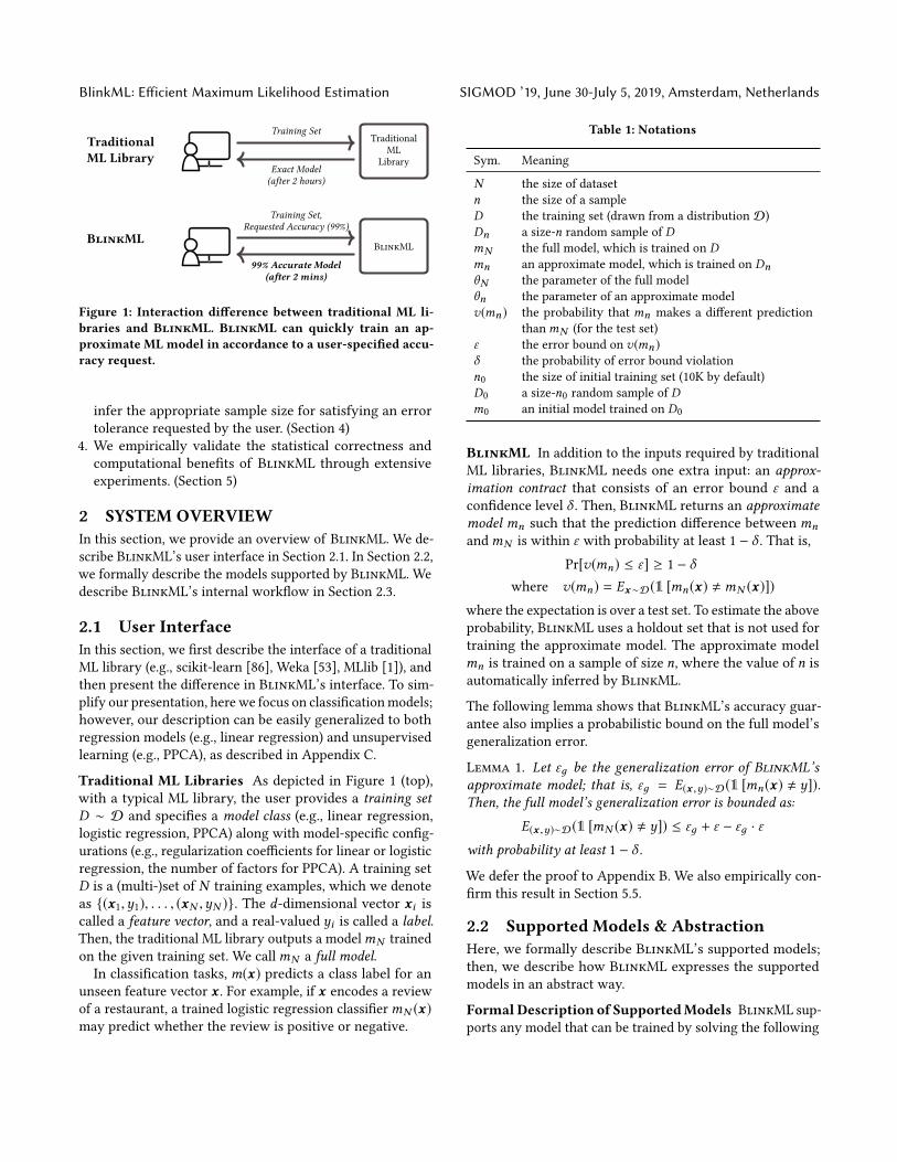
Figure 1: Interaction difference between traditional ML li-
braries and BlinkML. BlinkML can quickly train an ap-
proximate ML model in accordance to a user-specified accu-
racy request.
infer the appropriate sample size for satisfying an errortolerance requested by the user. (Section 4)
4. We empirically validate the statistical correctness andcomputational benefits of BlinkML through extensiveexperiments. (Section 5)
2 SYSTEM OVERVIEW
In this section, we provide an overview of BlinkML. We de-scribe BlinkML’s user interface in Section 2.1. In Section 2.2,we formally describe the models supported by BlinkML. Wedescribe BlinkML’s internal workflow in Section 2.3.
2.1 User Interface
In this section, we first describe the interface of a traditionalML library (e.g., scikit-learn [86], Weka [53], MLlib [1]), andthen present the difference in BlinkML’s interface. To sim-plify our presentation, here we focus on classificationmodels;however, our description can be easily generalized to bothregression models (e.g., linear regression) and unsupervisedlearning (e.g., PPCA), as described in Appendix C.
Traditional ML Libraries As depicted in Figure 1 (top),with a typical ML library, the user provides a training set
D ∼ D and specifies a model class (e.g., linear regression,logistic regression, PPCA) along with model-specific config-urations (e.g., regularization coefficients for linear or logisticregression, the number of factors for PPCA). A training setD is a (multi-)set of N training examples, which we denoteas (x1,y1), . . . , (xN ,yN ). The d-dimensional vector xi iscalled a feature vector, and a real-valued yi is called a label.Then, the traditional ML library outputs a modelmN trainedon the given training set. We callmN a full model.In classification tasks,m(x) predicts a class label for an
unseen feature vector x . For example, if x encodes a reviewof a restaurant, a trained logistic regression classifiermN (x)may predict whether the review is positive or negative.
Table 1: Notations
Sym. Meaning
N the size of datasetn the size of a sampleD the training set (drawn from a distribution D)Dn a size-n random sample of DmN the full model, which is trained on Dmn an approximate model, which is trained on DnθN the parameter of the full modelθn the parameter of an approximate modelv(mn ) the probability that mn makes a different prediction
thanmN (for the test set)ε the error bound on v(mn )
δ the probability of error bound violationn0 the size of initial training set (10K by default)D0 a size-n0 random sample of Dm0 an initial model trained on D0
BlinkML In addition to the inputs required by traditionalML libraries, BlinkML needs one extra input: an approx-
imation contract that consists of an error bound ε and aconfidence level δ . Then, BlinkML returns an approximate
model mn such that the prediction difference betweenmnandmN is within ε with probability at least 1 − δ . That is,
Pr[v(mn) ≤ ε] ≥ 1 − δ
where v(mn) = Ex∼D(1 [mn(x) ,mN (x)])
where the expectation is over a test set. To estimate the aboveprobability, BlinkML uses a holdout set that is not used fortraining the approximate model. The approximate modelmn is trained on a sample of size n, where the value of n isautomatically inferred by BlinkML.
The following lemma shows that BlinkML’s accuracy guar-antee also implies a probabilistic bound on the full model’sgeneralization error.
Lemma 1. Let εд be the generalization error of BlinkML’s
approximate model; that is, εд = E(x ,y)∼D(1 [mn(x) , y]).Then, the full model’s generalization error is bounded as:
E(x ,y)∼D(1 [mN (x) , y]) ≤ εд + ε − εд · ε
with probability at least 1 − δ .
We defer the proof to Appendix B. We also empirically con-firm this result in Section 5.5.
2.2 Supported Models & Abstraction
Here, we formally describe BlinkML’s supported models;then, we describe how BlinkML expresses the supportedmodels in an abstract way.
Formal Description of SupportedModels BlinkML sup-ports any model that can be trained by solving the following
SIGMOD ’19, June 30-July 5, 2019, Amsterdam, Netherlands Yongjoo Park, Jingyi Qing, Xiaoyang Shen, Barzan Mozafari
Model
Trainer
Model
Accuracy
Estimator
Sample
Size
Estimator
BlinkML Coordinator
Training
Set
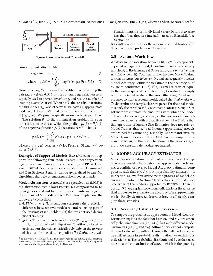
Figure 2: Architecture of BlinkML.
convex optimization problem:
arg minθ fn(θ ) (1)
where fn(θ ) =1n
n∑i=1
− log Pr(xi ,yi ; θ ) + R(θ ) (2)
Here, Pr(xi ,yi ; θ ) indicates the likelihood of observing thepair (xi , yi ) given θ , R(θ ) is the optional regularization termtypically used to prevent overfitting, and n is the number oftraining examples used. When n=N , this results in trainingthe full modelmN , and otherwise we have an approximatemodelmn . Different ML models use different expressions forPr(xi ,yi ; θ ). We provide specific examples in Appendix A.The solution θn to the minimization problem in Equa-
tion (1) is a value of θ at which the gradient дn(θ ) = ∇fn(θ )of the objective function fn(θ ) becomes zero.2 That is,
дn(θn) =
[1n
n∑i=1
q(θn ;xi ,yi )
]+ r (θn) = 0 (3)
where q(θ ;xi ,yi ) denotes −∇θ log Pr(xi ,yi ;θ ) and r (θ ) de-notes ∇θR(θ ).
Examples of Supported Models BlinkML currently sup-ports the following four model classes: linear regression,logistic regression, max entropy classifier, and PPCA. How-ever, BlinkML’s core technical contributions (Theorems 1and 2 in Sections 3 and 4) can be generalized to any MLalgorithms that rely on maximum likelihood estimation.
Model Abstraction A model class specification (MCS) isthe abstraction that allows BlinkML’s components to re-main generic and not tied to the specific internal logic ofthe supported ML models. Each MCS must implement thefollowing two methods:1. diff(m1, m2): This function computes the prediction
difference between two modelsm1 andm2, using part ofthe training set (i.e., holdout set) that was not used duringmodel training.
2. grads: This function returns a list of q(θ ;xi ,yi ) + r (θ ) fori = 1, . . . ,n, as defined in Equation (3). Although iterativeoptimization algorithms typically rely only on the averageof this list of values (i.e., the gradient ∇θ fn(θ )), the grads
2 In this work, we assume θn has fully converged to the optimal point, satisfyingEquation (3). The non-fully converged cases can be handled by simply adding smallerror terms to the diagonal elements of J in Theorem 1.
function must return individual values (without averag-ing them), as they are internally used by BlinkML (seeSection 3.4).
BlinkML already includes the necessary MCS definitions forthe currently supported model classes.
2.3 SystemWorkflow
We describe the workflow between BlinkML’s componentsdepicted in Figure 2. First, Coordinator obtains a size-n0sampleD0 of the training setD. We callD0 the initial trainingset (10K by default). Coordinator then invokes Model Trainerto train an initial modelm0 on D0, and subsequently invokesModel Accuracy Estimator to estimate the accuracy ε0 ofm0 (with confidence 1 − δ ). If ε0 is smaller than or equalto the user-requested error bound ε , Coordinator simplyreturns the initial model to the user. Otherwise, Coordinatorprepares to train a second model, called the final modelmn .To determine the sample size n required for the final modelto satisfy the error bound, Coordinator consults Sample SizeEstimator to estimate the smallest n with which the modeldifference betweenmn andmN (i.e., the unknown full model)would not exceed ε with probability at least 1 − δ . Note thatthis operation of Sample Size Estimator does not rely onModel Trainer; that is, no additional (approximate) modelsare trained for estimating n. Finally, Coordinator invokesModel Trainer (for a second time) to train on a sample of sizen and returnmn to the user. Therefore, in the worst case, atmost two approximate models are trained.
3 MODEL ACCURACY ESTIMATOR
Model Accuracy Estimator estimates the accuracy of an ap-proximate model. That is, given an approximate modelmnand a confidence level δ , Model Accuracy Estimator com-putes ε , such that v(mn) ≤ ε with probability at least 1 − δ .In Section 3.1, we first overview the process of Model Ac-curacy Estimator. In Section 3.2, we establish the statisticalproperties of the models supported by BlinkML. Then, inSection 3.3, we explain how BlinkML exploits these statis-tical properties to estimate the accuracy of an approximatemodel. Finally, Section 3.4 describes how to efficiently com-pute those statistics.
3.1 Accuracy Estimation Overview
To compute the probabilistic upper bound ε , Model AccuracyEstimator exploits the fact that bothmn andmN are essen-tially the same function (i.e.,m(x)) but with different modelparameters (i.e., θn and θN ). Although we cannot computethe exact value of θN without training the full modelmN , wecan still estimate its probability distribution (we explain thisin Section 3.2). The probability distribution of θN is then usedto estimate the distribution of v(mn), which is the quantity

BlinkML: Efficient Maximum Likelihood Estimation SIGMOD ’19, June 30-July 5, 2019, Amsterdam, Netherlands
θ
θN θn
д(θN )
д(θn )
α J
α H−1 JH−1
slope = H
Figure 3: The variances α H−1 JH−1of sampling-based model
parameters are obtained using two model/data-aware quan-
tities (i.e., α J and H ).
we aim to upper bound. The upper bound ε is determinedby simply finding the value that is larger than v(mn) for100 · (1 − δ )% of the holdout examples. (Section 3.3).
3.2 Model Parameter Distribution
In this section, we present how to probabilistically expressthe parameter θN of the (unknown) full model mN givenonly the parameter θn of an approximate modelmn . Let θnbe a random variable representing the distribution of theapproximate model’s parameters; θn is simply one instanceof θn . We also use θN to represent our (limited) knowledgeof θN . Then, our goal is to obtain the distribution of θn − θN ,and then use this distribution to estimate the predictiondifference betweenm(θn) andm(θN ).
Intuition Since θn is the value that satisfies Equation (3)for n training examples (instead of N ), we can obtain thedifference α J between дn(θn) and дN (θN ). In addition, wecan obtain the relationship H between дn(θn) − дN (θN ) andθn − θN using the Taylor expansion of дn(θ ). Then, we canfinally derive the difference between θn and θN .Figure 3 depicts this idea intuitively. In the figure, the
slopeH captures the surface of the gradient, and α J capturesthe variance of the gradient; α J decreases as n increases.Thus, if a model is more flexible (e.g., smaller regularizationcoefficients), the slope becomes more moderate (i.e., smallerelements in H ), which leads to a larger distance between θNand θn given the same α J . In other words, the approximatemodel will be less accurate given a fixed sample size. Below,we formally present this idea. To account for these differ-ences between models, BlinkML automatically adjusts itssample size n when it trains an approximate model to satisfythe requested error bound (Section 4).
Parameter Distribution The following theorem providesthe distribution of θn − θN (its proof is in Appendix B).
Theorem 1. Let J be the Jacobian of дn(θ ) − r (θ ) evaluated atθn , and let H be the Jacobian of дn(θ ) evaluated at θn . Then,
θn − θN → N(0, α H−1 JH−1), α =1n−
1N
as n → ∞ and N → ∞. N denotes a normal distribution,
which means that θn − θN asymptotically follows a multivari-
ate normal distribution with covariance matrix α H−1 JH−1.
Directly computing H and J requires Ω(d2) space where dis the number of features. This can be prohibitively expensivewhen d is large. To address this, these quantities are indi-rectly computed (as described in Section 3.4 and Section 4.3),reducing the computational cost to onlyO(d). Our empiricalstudy shows that BlinkML can scale up to datasets with amillion features (Section 5).
In Theorem 1, J is essentially the covariance matrix of gra-dients (computed on individual examples). Since BlinkMLuses uniform random sampling, estimating J is simpler; how-ever, even when non-uniform random sampling is used, Jcan still be estimated if we know the sampling probabilities.By assigning those sampling probabilities in a task-specificway, one could obtain higher accuracy, which we leave asfuture work.
The following corollary provides the conditional distribu-tion of θN | θn (proof in Appendix B).
Corollary 1. Without any a priori knowledge of θN ,
θN | θn → N(θn , α H−1 JH−1), α =1n−
1N
as n → ∞ and N → ∞.
The following section uses the conditional distributionθN | θn (in Corollary 1) to obtain an error bound on theapproximate model.
3.3 Error Bound on Approximate Model
In this section, we describe how Model Accuracy Estimatorestimates the accuracy of an approximate modelmn . Specifi-cally, we show how to estimate v(mn) without trainingmN .Let h(θN ) denote the probability density function of the
normal distribution with mean θn and covariance matrixαH−1 JH−1 (obtained in Corollary 1). Then, we aim to findthe error bound ε of an approximate model that holds withprobability at least 1 − δ . That is,
PrθN [v(mn) ≤ ε] ≥ 1 − δ where
PrθN [v(mn) ≤ ε] =
∫1 [v(mn ;θN ) ≤ ε] h(θN ) dθN , (4)
mn(x) =m(x ; θn), mN (x) =m(x ; θN | θn)
where the integration is over the domain of θN (∈ Rd );v(mn ;θN ) is the error ofmn when the full model’s parameter
SIGMOD ’19, June 30-July 5, 2019, Amsterdam, Netherlands Yongjoo Park, Jingyi Qing, Xiaoyang Shen, Barzan Mozafari
is θN ; and 1 [·] is the indicator function that returns 1 if itsargument is true and returns 0 otherwise. Since the above ex-pression involves the model’s (blackbox) prediction functionm(x), it cannot be analytically computed in general.
To compute Equation (4), BlinkML’s Model Accuracy Es-timator uses the empirical distribution of h(θN ) as follows.Let θN ,1, . . . ,θN ,k be i.i.d. samples drawn from h(θN ). Then,∫
1 [v(mn ;θN ) ≤ ε] h(θN ) dθN ≈1k
k∑i=1
1[v(mn ;θN ,i ) ≤ ε
](5)
To take into account the approximation error in Equation (5),BlinkML uses conservative estimates on ε as formally statedin the following lemma (see Appendix B for proof).
Lemma 2. If ε satisfies
1k
k∑i=1
1[v(mn ;θN ,i ) ≤ ε
]=
1 − δ
0.95+
√log 0.95
−2k
then Pr[v(mn) ≤ ε] ≥ 1 − δ .
The above lemma implies that by using a larger k (i.e., num-ber of sampled values), we can obtain a tighter ε . To obtaina large k , an efficient sampling algorithm is necessary. SinceθN follows a normal distribution, one can simply use an exist-ing library, such as numpy.random. However, BlinkML usesits own fast, custom sampler to avoid directly computing thecovariance matrix H−1 JH−1 (see Section 4.3).
3.4 Computing Necessary Statistics
We present three methods—(1) ClosedForm, (2) InverseG-radients, and (3) ObservedFisher—for computing H . GivenH , computing J is straightforward since J = H − Jr , whereJr is the Jacobian of r (θ ). BlinkML uses ObservedFisher bydefault since it achieves high memory-efficiency by avoidingthe direct computations of H .
Method 1: ClosedForm ClosedFormuses the analytic formof the Jacobian H (θ ) of дn(θ ), and sets θ = θn by the defi-nition of H . For instance, H (θ ) of L2-regularized logisticregression is expressed as follows:
H (θ ) =1nX⊤QX + βI
where X is an n-by-d matrix whose i-th row is xi , and Qis a d-by-d diagonal matrix whose i-th diagonal entry isσ (θ⊤xi )(1 − σ (θ⊤xi )), and β is the coefficient of L2 regular-ization. When H (θ ) is available, as in the case of logisticregression, ClosedForm is fast and exact.
However, inverting H is computationally expensive whend is large. Also, using ClosedForm is less straightforwardwhen obtaining analytic expression of H (θ ) is non-trivial.
Method 2: InverseGradients InverseGradients numeri-cally computes H by relying on the Taylor expansion ofдn(θ ): дn(θn + dθ ) ≈ дn(θn) + Hdθ . Since дn(θn) = 0, theTaylor expansion simplifies to:
дn(θn + dθ ) ≈ Hdθ
The values of дn(θn + dθ ) and дn(θn) are computed usingthe grads function provided by the MCS. The remainingquestion is what values of dθ to use for computing H . SinceH is a d-by-d matrix, BlinkML uses d number of linearlyindependent dθ to fully construct H . That is, let P be ϵI ,where ϵ is a small real number (10−6 by default). Also, letR be the d-by-d matrix whose i-th column is дn(θn + P ·,i )where P ·,i is the i-th column of P . Then, H ≈ RP−1.
Since InverseGradients only relies on the grads function,it is applicable to all supported models. Although InverseG-radients is accurate, it is still computationally inefficient forhigh-dimensional data, since the grads function must becalled d times. We study its runtime overhead in Section 5.6.
Method 3: ObservedFisher ObservedFisher numericallycomputes H by relying on the information matrix equal-ity [77].3 According to the information matrix equality, thecovariance matrixC ofq(θn ;xi ,yi ), for i = 1, . . . ,n, is asymp-totically identical to J (i.e., as n → ∞). In addition, given J ,we can simply obtain H as H = C + Jr . Our empirical studyin Section 5.6 shows that ObservedFisher is highly accuratefor n ≥ 5K .Instead of computing the d-by-d matrix C directly, Ob-
servedFisher takes a slightly different approach. That is,ObservedFisher computes factors U and Σ such that C =U Σ2U ⊤, where U is a d-by-n matrix, and Σ is an n-by-ndiagonal matrix. As described below, this factor-based ap-proach is significantly more efficient when d is large, henceallowing BlinkML to scale up to high-dimensional data.Specifically, let Q be the n-by-d matrix whose i-th row
is q(θn ;xi ,yi ). Then, ObservedFisher performs the singularvalue decomposition of Q⊤ to obtainU , Σ, and V such thatQ⊤ = U ΣV⊤. Then, the following relationship holds:
C = Q⊤Q = U Σ2U ⊤ (6)
As stated above, ObservedFisher never computes C; it onlystoresU and Σ, which are used directly for obtaining samplesfrom N(0,H−1 JH−1) (see Section 4.3). The cost of singularvalue decomposition is O(min(n2d,nd2)). When d ≥ n, thistime complexity becomes O(n2d) = O(d) for a fixed sam-ple size (n0 = 10K by default). Moreover, ObservedFisherrequires only a single call of the grads function. Section 5.6empirically studies the relationship between n and Observed-Fisher’s runtime.
3ObservedFisher is also inspired by Hessian-free optimizations [69, 72].
BlinkML: Efficient Maximum Likelihood Estimation SIGMOD ’19, June 30-July 5, 2019, Amsterdam, Netherlands
θ0
θnθN
θn
θNsample #1sample #2
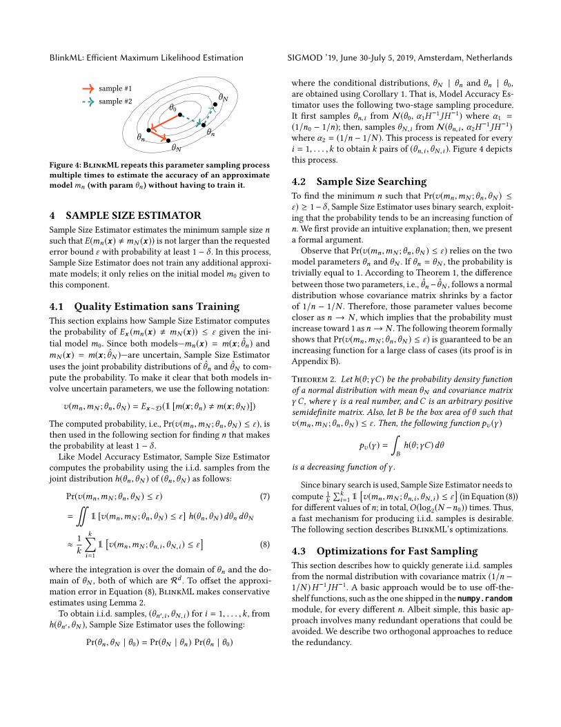
Figure 4: BlinkML repeats this parameter sampling process
multiple times to estimate the accuracy of an approximate
modelmn (with param θn ) without having to train it.
4 SAMPLE SIZE ESTIMATOR
Sample Size Estimator estimates the minimum sample size nsuch that E(mn(x) ,mN (x)) is not larger than the requestederror bound ε with probability at least 1 − δ . In this process,Sample Size Estimator does not train any additional approxi-mate models; it only relies on the initial modelm0 given tothis component.
4.1 Quality Estimation sans Training
This section explains how Sample Size Estimator computesthe probability of Ex (mn(x) , mN (x)) ≤ ε given the ini-tial model m0. Since both models—mn(x) = m(x ; θn) andmN (x) = m(x ; θN )—are uncertain, Sample Size Estimatoruses the joint probability distributions of θn and θN to com-pute the probability. To make it clear that both models in-volve uncertain parameters, we use the following notation:
v(mn ,mN ;θn ,θN ) = Ex∼D(1 [m(x ;θn) ,m(x ;θN )])
The computed probability, i.e., Pr(v(mn ,mN ;θn ,θN ) ≤ ε), isthen used in the following section for finding n that makesthe probability at least 1 − δ .Like Model Accuracy Estimator, Sample Size Estimator
computes the probability using the i.i.d. samples from thejoint distribution h(θn ,θN ) of (θn ,θN ) as follows:
Pr(v(mn ,mN ;θn ,θN ) ≤ ε) (7)
=
∬1 [v(mn ,mN ;θn ,θN ) ≤ ε] h(θn ,θN )dθn dθN
≈1k
k∑i=1
1[v(mn ,mN ;θn,i ,θN ,i ) ≤ ε
](8)
where the integration is over the domain of θn and the do-main of θN , both of which are Rd . To offset the approxi-mation error in Equation (8), BlinkML makes conservativeestimates using Lemma 2.To obtain i.i.d. samples, (θn′,i ,θN ,i ) for i = 1, . . . ,k , from
h(θn′,θN ), Sample Size Estimator uses the following:
Pr(θn ,θN | θ0) = Pr(θN | θn) Pr(θn | θ0)
where the conditional distributions, θN | θn and θn | θ0,are obtained using Corollary 1. That is, Model Accuracy Es-timator uses the following two-stage sampling procedure.It first samples θn,i from N(θ0, α1H
−1 JH−1) where α1 =
(1/n0 − 1/n); then, samples θN ,i from N(θn,i , α2H−1 JH−1)
where α2 = (1/n − 1/N ). This process is repeated for everyi = 1, . . . ,k to obtain k pairs of (θn,i ,θN ,i ). Figure 4 depictsthis process.
4.2 Sample Size Searching
To find the minimum n such that Pr(v(mn ,mN ;θn ,θN ) ≤
ε) ≥ 1−δ , Sample Size Estimator uses binary search, exploit-ing that the probability tends to be an increasing function ofn. We first provide an intuitive explanation; then, we presenta formal argument.Observe that Pr(v(mn ,mN ;θn ,θN ) ≤ ε) relies on the two
model parameters θn and θN . If θn = θN , the probability istrivially equal to 1. According to Theorem 1, the differencebetween those two parameters, i.e., θn−θN , follows a normaldistribution whose covariance matrix shrinks by a factorof 1/n − 1/N . Therefore, those parameter values becomecloser as n → N , which implies that the probability mustincrease toward 1 asn → N . The following theorem formallyshows that Pr(v(mn ,mN ;θn ,θN ) ≤ ε) is guaranteed to be anincreasing function for a large class of cases (its proof is inAppendix B).
Theorem 2. Let h(θ ;γC) be the probability density function
of a normal distribution with mean θN and covariance matrix
γ C , where γ is a real number, and C is an arbitrary positive
semidefinite matrix. Also, let B be the box area of θ such that
v(mn ,mN ;θn ,θN ) ≤ ε . Then, the following function pv (γ )
pv (γ ) =
∫Bh(θ ;γC)dθ
is a decreasing function of γ .
Since binary search is used, Sample Size Estimator needs tocompute 1
k∑k
i=1 1[v(mn ,mN ;θn,i ,θN ,i ) ≤ ε
](in Equation (8))
for different values of n; in total,O(log2(N −n0)) times. Thus,a fast mechanism for producing i.i.d. samples is desirable.The following section describes BlinkML’s optimizations.
4.3 Optimizations for Fast Sampling
This section describes how to quickly generate i.i.d. samplesfrom the normal distribution with covariance matrix (1/n −
1/N )H−1 JH−1. A basic approach would be to use off-the-shelf functions, such as the one shipped in the numpy.randommodule, for every different n. Albeit simple, this basic ap-proach involves many redundant operations that could beavoided. We describe two orthogonal approaches to reducethe redundancy.
SIGMOD ’19, June 30-July 5, 2019, Amsterdam, Netherlands Yongjoo Park, Jingyi Qing, Xiaoyang Shen, Barzan Mozafari
Sampling by Scaling We can avoid invoking a samplingfunction multiple times for differentn by exploiting the struc-tural similarity of the covariance matrices associated withdifferent n. Let θn ∼ N(0, (1/n − 1/N )H−1 JH−1), and letθ0 ∼ N(0, H−1 JH−1). Then, there exists the following rela-tionship:
θn =√
1/n − 1/N θ0.
This indicates that we can first draw i.i.d. samples fromthe unscaled distributionN(0,H−1 JH−1); then, we can scalethose sampled values by
√1/n − 1/N whenever the i.i.d. sam-
ples from N(0, (1/n − 1/N )H−1 JH−1) are needed.
AvoidingDirect Covariance Computation When r (θ ) =βθ in Equation (3) (i.e., no regularization or L2 regulariza-tion), Sample Size Estimator avoids the direct computationsof H−1 JH−1. Instead, it simply draws samples from the stan-dard normal distribution and applies an appropriate lineartransformation L to the sampled values (L is obtained shortly).This approach is used in conjunction with ObservedFisher,which is BlinkML’s default strategy for computing its nec-essary statistics (Section 3.4).Avoiding the direct computation of the covariances has
two benefits. First, we can completely avoid the Ω(d2) costof computing/storing H−1 JH−1. Second, sampling from thestandard normal distribution is much faster because no de-pendencies need to be enforced among sampled values.
We use the following relationship:
z ∼ N(0, I ) ⇒ L z ∼ N(0, L L⊤).
That is, if there exists L such that L L⊤ = H−1 JH−1, we canobtain the samples of θ0 by multiplying L to the samplesdrawn from the standard normal distribution.
Specifically, Sample Size Estimator performs the followingfor obtaining L. Observe from Equation (6) that J = U Σ2U ⊤.Since H = J + β , H = U (Σ2 + βI )U ⊤. Thus,
H−1 JH−1 = U (Σ2 + βI )−1U ⊤ U Σ2U ⊤ U (Σ2 + βI )−1U ⊤
⇒ H−1 JH−1 = (UΛ) (UΛ)⊤ = L L⊤
where Λ is a diagonal matrix whose i-th diagonal entry issi/(s
2i + β), where si is the i-th singular value of J contained
in Σ. Note that both U and Σ are already available as partof computing the necessary statistics in Section 3.4. Thus,computing L only involves a simple matrix multiplication.
5 EXPERIMENTS
Our experimental results show the following:1. BlinkML reduces training time by 84.04%–99.84% (i.e.,
6.26×–629×) when training 95% accurate models. and by7.20%–96.47% (i.e., 1.07×–28.31× faster) when training 99%accurate models. (Section 5.2)
Table 2: Datasets used in our experiments
Dataset # of Rows (N ) Dimension (d) Size
Gas 4,178,504 57 1.9 GBPower 2,075,259 114 1.8 GBCriteo 45,840,616 998,922 2.86 GBHIGGS 11,000,000 28 7.5 GBMNIST 8,000,000 784 47.5 GBYelp 5,261,667 100,000 487 MB
2. The actual accuracy of BlinkML’s approximate modelsis, in most cases, even higher than the requested accuracy.(Section 5.3)
3. BlinkML’s estimated minimum sample sizes are close tooptimal. (Section 5.4)
4. BlinkML is highly effective and accurate even for high-dimensional data, and its runtime overhead ismuch smallerthan the time needed for training a full model. (Section 5.5)
5. BlinkML’s default statistics computation method, Ob-servedFisher, is both accurate and efficient. (Section 5.6)
6. BlinkML offers significant benefits in hyperparameteroptimization compared to full model training. (Section 5.7)
7. BlinkML’s sample size estimation is adaptive to the prop-erties of models. (Section 5.8)
5.1 Experiment Setup
Here, we present our computational environment as well asthe different models and datasets used in our experiments.
Models We tested BlinkML with four different ML models:1. Linear Regression (Lin). Lin is the standard linear re-
gression model with L2 regularization coefficient β set as0.001. Different values of β are tested in Section 5.8.
2. Logistic Regression (LR). LR is the standard logistic re-gression (binary) classifier with L2-regularization coeffi-cient β set as 0.001.
3. Max Entropy Classifier (ME). ME is the standard maxentropy (multiclass) classifier with L2-regularization coef-ficient β set as 0.001.
4. PPCA. PPCA is the standard probabilistic principal com-ponent analysis model [99], with the number of factors qset as 10.
BlinkML is configured to use the BFGS optimization al-gorithm for low-dimensional datasets (d < 100) and touse a memory-efficient alternative, called L-BFGS, for high-dimensional datasets (d ≥ 100).
Datasets We used six real-world datasets. The key charac-teristics of these datasets are summarized in Table 2.Linear Regression:
1. Gas: This dataset contains chemical sensor readings ex-posed to gas mixtures at varying concentration levels [44].
BlinkML: Efficient Maximum Likelihood Estimation SIGMOD ’19, June 30-July 5, 2019, Amsterdam, Netherlands
0%20%40%60%80%100%
Speedup (left Y-axis) Time Saving (right Y-axis)80%
85%
90%
95%
96%
97%
98%
99%
100%
1×10×100×103×
104×
Requested Accuracy ((1 − ε ) × 100%)
(a) Lin, Gas
0%20%40%60%80%100%
80%
85%
90%
95%
96%
97%
98%
99%
100%
1×
10×
100×
103×
Requested Accuracy ((1 − ε ) × 100%)
(b) LR, Criteo
0%20%40%60%80%100%
80%
85%
90%
95%
96%
97%
98%
99%
100%
1×
10×
100×
103×
Requested Accuracy ((1 − ε ) × 100%)
(c) ME, MNIST
0%20%40%60%80%100%
90%
95%
99%
99.5%
99.9%
99.95%
99.99%
100%
1×
10×
100×
Requested Accuracy ((1 − ε ) × 100%)
(d) PPCA, MNIST
0%20%40%60%80%100%
80%
85%
90%
95%
96%
97%
98%
99%
100%
1×
10×
100×
103×
Requested Accuracy ((1 − ε ) × 100%)
(e) Lin, Power
0%20%40%60%80%100%
80%
85%
90%
95%
96%
97%
98%
99%
100%
1×10×100×103×
104×
Requested Accuracy ((1 − ε ) × 100%)
(f) LR, HIGGS
0%20%40%60%80%100%
80%
85%
90%
95%
96%
97%
98%
99%
100%
1×
10×
100×
Requested Accuracy ((1 − ε ) × 100%)
(g) ME, Yelp
0%20%40%60%80%100%
90%
95%
99%
99.5%
99.9%
99.95%
99.99%
100%
1×
10×
100×
Requested Accuracy ((1 − ε ) × 100%)
(h) PPCA, HIGGS
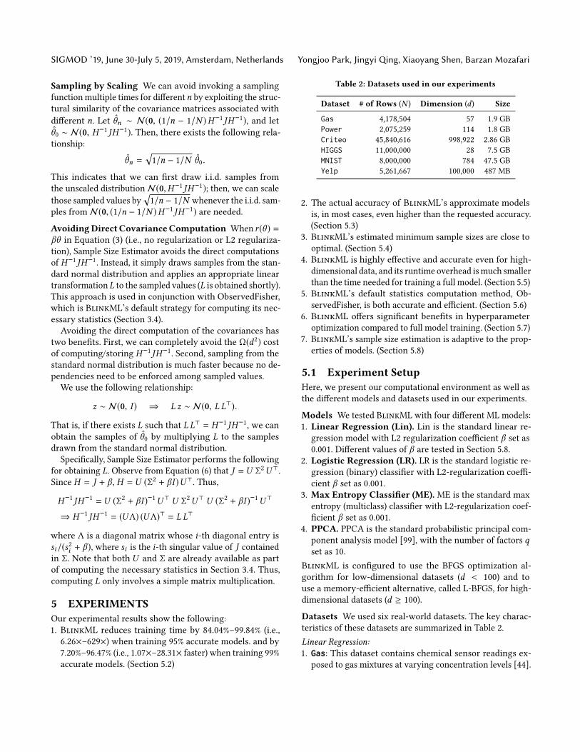
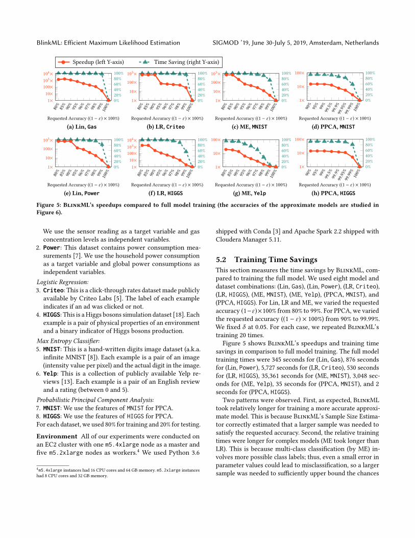
Figure 5: BlinkML’s speedups compared to full model training (the accuracies of the approximate models are studied in
Figure 6).
We use the sensor reading as a target variable and gasconcentration levels as independent variables.
2. Power: This dataset contains power consumption mea-surements [7]. We use the household power consumptionas a target variable and global power consumptions asindependent variables.
Logistic Regression:
3. Criteo: This is a click-through rates dataset made publiclyavailable by Criteo Labs [5]. The label of each exampleindicates if an ad was clicked or not.
4. HIGGS: This is a Higgs bosons simulation dataset [18]. Eachexample is a pair of physical properties of an environmentand a binary indicator of Higgs bosons production.
Max Entropy Classifier:
5. MNIST: This is a hand-written digits image dataset (a.k.a.infinite MNIST [8]). Each example is a pair of an image(intensity value per pixel) and the actual digit in the image.
6. Yelp: This is a collection of publicly available Yelp re-views [13]. Each example is a pair of an English reviewand a rating (between 0 and 5).
Probabilistic Principal Component Analysis:
7. MNIST: We use the features of MNIST for PPCA.8. HIGGS: We use the features of HIGGS for PPCA.For each dataset, we used 80% for training and 20% for testing.
Environment All of our experiments were conducted onan EC2 cluster with one m5.4xlarge node as a master andfive m5.2xlarge nodes as workers.4 We used Python 3.6
4m5.4xlarge instances had 16 CPU cores and 64 GB memory. m5.2xlarge instanceshad 8 CPU cores and 32 GB memory.
shipped with Conda [3] and Apache Spark 2.2 shipped withCloudera Manager 5.11.
5.2 Training Time Savings
This section measures the time savings by BlinkML, com-pared to training the full model. We used eight model anddataset combinations: (Lin, Gas), (Lin, Power), (LR, Criteo),(LR, HIGGS), (ME, MNIST), (ME, Yelp), (PPCA, MNIST), and(PPCA, HIGGS). For Lin, LR and ME, we varied the requestedaccuracy (1−ε)×100% from 80% to 99%. For PPCA, we variedthe requested accuracy ((1 − ε) × 100%) from 90% to 99.99%.We fixed δ at 0.05. For each case, we repeated BlinkML’straining 20 times.Figure 5 shows BlinkML’s speedups and training time
savings in comparison to full model training. The full modeltraining times were 345 seconds for (Lin, Gas), 876 secondsfor (Lin, Power), 5,727 seconds for (LR, Criteo), 530 secondsfor (LR, HIGGS), 35,361 seconds for (ME, MNIST), 3,048 sec-onds for (ME, Yelp), 35 seconds for (PPCA, MNIST), and 2seconds for (PPCA, HIGGS).
Two patterns were observed. First, as expected, BlinkMLtook relatively longer for training a more accurate approxi-mate model. This is because BlinkML’s Sample Size Estima-tor correctly estimated that a larger sample was needed tosatisfy the requested accuracy. Second, the relative trainingtimes were longer for complex models (ME took longer thanLR). This is because multi-class classification (by ME) in-volves more possible class labels; thus, even a small error inparameter values could lead to misclassification, so a largersample was needed to sufficiently upper bound the chances
SIGMOD ’19, June 30-July 5, 2019, Amsterdam, Netherlands Yongjoo Park, Jingyi Qing, Xiaoyang Shen, Barzan Mozafari
80%85%90%95%96%97%98%99%
85%90%95%100%
Requested Accuracy ((1 − ε ) × 100%)
ActualA
ccuracy
Actual Accuracy Mean Actual Accuracy 5th Percentile Requested Accuracy
(a) Lin, Gas
80%85%90%95%96%97%98%99%
85%90%95%100%
Requested Accuracy ((1 − ε ) × 100%)
ActualA
ccuracy
(b) LR, Criteo
80%85%90%95%96%97%98%99%
85%90%95%100%
Requested Accuracy ((1 − ε ) × 100%)
ActualA
ccuracy
(c) ME, MNIST
90% 95% 99%99.5%99.9
%99.9
5%99.9
9%95%96%97%98%99%100%
Requested Accuracy ((1 − ε ) × 100%)
ActualA
ccuracy
(d) PPCA, MNIST
80%85%90%95%96%97%98%99%
85%90%95%100%
Requested Accuracy ((1 − ε ) × 100%)
ActualA
ccuracy
(e) Lin, Power
80%85%90%95%96%97%98%99%
85%90%95%100%
Requested Accuracy ((1 − ε ) × 100%)
ActualA
ccuracy
(f) LR, HIGGS
80%85%90%95%96%97%98%99%
85%90%95%100%
Requested Accuracy ((1 − ε ) × 100%)
ActualA
ccuracy
(g) ME, Yelp
90% 95% 99%99.5%99.9
%99.9
5%99.9
9%95%96%97%98%99%100%
Requested Accuracy ((1 − ε ) × 100%)
ActualA
ccuracy
(h) PPCA, HIGGS
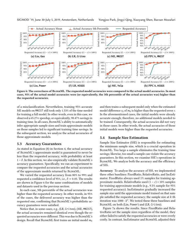
Figure 6: The correctness of BlinkML. The requestedmodel accuracies were compared to the actual model accuracies. Inmost
cases, 95% of the actual model accuracies were (or equivalently, the 5th percentile of the actual accuracies was) higher than
the requested accuracies.
of a misclassification. Nevertheless, training 95% accurateME models on MNIST still took only 1.53% of the time neededfor training a full model. In other words, even in this case, weobserved a 65.27× speedup, or equivalently, 98.47% savings intraining time. In all cases, BlinkML’s ability to automaticallyinfer appropriate sample sizes and train approximate modelson those samples led to significant training time savings. Inthe subsequent section, we analyze the actual accuracies ofthose approximate models.
5.3 Accuracy Guarantees
As stated in Equation (8) in Section 4, the actual accuracyof BlinkML’s approximate model is guaranteed to never beless than the requested accuracy, with probability at least1−δ . In this section, we also empirically validate BlinkML’saccuracy guarantees. Specifically, we ran an experiment tocompare the requested accuracies and the actual accuraciesof the approximate models returned by BlinkML.We varied the requested accuracy from 80% to 99% and
requested a confidence level of 95%, i.e., δ = 0.05. The resultsare shown in Figure 6 for the same combinations of modelsand datasets used in the previous section.In each case, 5th percentile of the actual accuracies was
higher than the requested accuracy. In other words, in 95%of the cases, the delivered accuracy was higher than therequested one, confirming that BlinkML’s probabilistic ac-curacy guarantees were satisfied.
Notice that, in some cases, e.g., (LR, Criteo), (ME, MNIST),the actual accuracies remained identical even though the re-quested accuracieswere different. Thiswas due toBlinkML’sdesign. Recall that BlinkML first trains an initial modelm0
and then trains a subsequent model only when the estimatedmodel difference ε0 ofm0 is higher than the requested error ε .In the aforementioned cases, the initial models were alreadyaccurate enough; therefore, no additional models needed tobe trained. Consequently, the actual accuracies did not varyin those cases. In other words, the actual accuracies of thoseinitial models were higher than the requested accuracies.
5.4 Sample Size Estimation
Sample Size Estimator (SSE) is responsible for estimatingthe minimum sample size, which is a crucial operation inBlinkML. Too large a sample eliminates the training timesavings; likewise, too small a sample can violate the accuracyguarantees. In this section, we examine SSE’s operations inBlinkML. We analyze both the accuracy and the efficiencyof SSS.
Accuracy To analyze the accuracy of SSS, we implementedthree other baselines: FixedRatio, RelativeRatio, and IncEsti-mator. FixedRatio always used 1% samples for training ap-proximate models. RelativeRatio used (1 − ε) ∗ 10% samplesfor training approximate models (e.g., 9.5% sample for 95%requested accuracy). IncEstimator gradually increased thesample size until the approximate model trained on that sam-ple satisfied the requested accuracy; the sample size at k-thiteration was 1000 · k2. We tested these three baselines andBlinkML on both (Lin, Power) and (LR, Criteo).Figure 7a shows the results. Since FixedRatio and Rela-
tiveRatio set the sample sizes regardless of the model, theyeither failed to satisfy the requested accuracies or were overlycostly. In contrast, IncEstimator and BlinkML adjusted their
BlinkML: Efficient Maximum Likelihood Estimation SIGMOD ’19, June 30-July 5, 2019, Amsterdam, Netherlands
80% 85% 90% 95% 96% 97% 98% 99%92%
94%
96%
98%
100%
Lin, Power
Requested Accuracy
ActualA
ccuracy
FixedRatio RelativeRatio IncEstimator BlinkML BlinkML’s pure training time
80% 85% 90% 95% 96% 97% 98% 99%92%
94%
96%
98%
100%
LR, Criteo
Requested Accuracy
ActualA
ccuracy
(a) Effectiveness of Sample Size Estimator
80% 85% 90% 95% 96% 97% 98% 99%1
10
100
1KLin, Power
Requested Accuracy
Runtim
e(sec)
80% 85% 90% 95% 96% 97% 98% 99%1
10
1001K
10K
LR, Criteo
Requested Accuracy
Runtim
e(sec)
(b) Efficiency of Sample Size Estimator
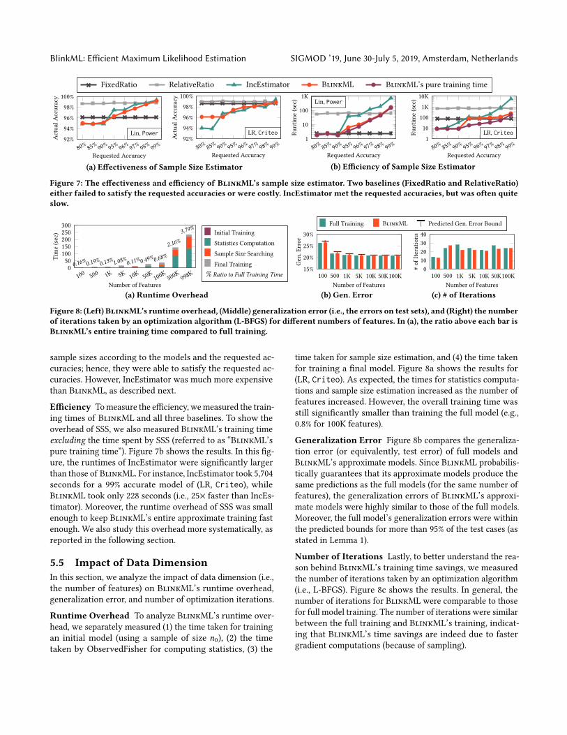
Figure 7: The effectiveness and efficiency of BlinkML’s sample size estimator. Two baselines (FixedRatio and RelativeRatio)
either failed to satisfy the requested accuracies or were costly. IncEstimator met the requested accuracies, but was often quite
slow.
100 500 1K 5K 10K 50K 100K500
K998
K0
50100150200250300
3.79%
2.16%
0.68%
0.49%
0.11%
1.08%
0.13%
0.19%
0.16%
Number of Features
Time(sec) Initial Training
Statistics ComputationSample Size SearchingFinal Training
% Ratio to Full Training Time
(a) Runtime Overhead
100 500 1K 5K 10K 50K100K15%
20%
25%
30%
Number of Features
Gen.E
rror
Full Training BlinkML Predicted Gen. Error Bound
(b) Gen. Error
100 500 1K 5K 10K 50K100K010203040
Number of Features
#of
Iteratio
ns
(c) # of Iterations
Figure 8: (Left)BlinkML’s runtime overhead, (Middle) generalization error (i.e., the errors on test sets), and (Right) the number
of iterations taken by an optimization algorithm (L-BFGS) for different numbers of features. In (a), the ratio above each bar is
BlinkML’s entire training time compared to full training.
sample sizes according to the models and the requested ac-curacies; hence, they were able to satisfy the requested ac-curacies. However, IncEstimator was much more expensivethan BlinkML, as described next.
Efficiency Tomeasure the efficiency, wemeasured the train-ing times of BlinkML and all three baselines. To show theoverhead of SSS, we also measured BlinkML’s training timeexcluding the time spent by SSS (referred to as “BlinkML’spure training time”). Figure 7b shows the results. In this fig-ure, the runtimes of IncEstimator were significantly largerthan those of BlinkML. For instance, IncEstimator took 5,704seconds for a 99% accurate model of (LR, Criteo), whileBlinkML took only 228 seconds (i.e., 25× faster than IncEs-timator). Moreover, the runtime overhead of SSS was smallenough to keep BlinkML’s entire approximate training fastenough. We also study this overhead more systematically, asreported in the following section.
5.5 Impact of Data Dimension
In this section, we analyze the impact of data dimension (i.e.,the number of features) on BlinkML’s runtime overhead,generalization error, and number of optimization iterations.
Runtime Overhead To analyze BlinkML’s runtime over-head, we separately measured (1) the time taken for trainingan initial model (using a sample of size n0), (2) the timetaken by ObservedFisher for computing statistics, (3) the
time taken for sample size estimation, and (4) the time takenfor training a final model. Figure 8a shows the results for(LR, Criteo). As expected, the times for statistics computa-tions and sample size estimation increased as the number offeatures increased. However, the overall training time wasstill significantly smaller than training the full model (e.g.,0.8% for 100K features).
Generalization Error Figure 8b compares the generaliza-tion error (or equivalently, test error) of full models andBlinkML’s approximate models. Since BlinkML probabilis-tically guarantees that its approximate models produce thesame predictions as the full models (for the same number offeatures), the generalization errors of BlinkML’s approxi-mate models were highly similar to those of the full models.Moreover, the full model’s generalization errors were withinthe predicted bounds for more than 95% of the test cases (asstated in Lemma 1).
Number of Iterations Lastly, to better understand the rea-son behind BlinkML’s training time savings, we measuredthe number of iterations taken by an optimization algorithm(i.e., L-BFGS). Figure 8c shows the results. In general, thenumber of iterations for BlinkML were comparable to thosefor full model training. The number of iterations were similarbetween the full training and BlinkML’s training, indicat-ing that BlinkML’s time savings are indeed due to fastergradient computations (because of sampling).
SIGMOD ’19, June 30-July 5, 2019, Amsterdam, Netherlands Yongjoo Park, Jingyi Qing, Xiaoyang Shen, Barzan Mozafari
100 500 1K 5K 10K 50K 100K0.5
1
1.5
2
Optimal Ratio
Sample Size
Est.Va
r/ActualV
ar
ClosedFormInverseGradientsObservedFisher
(a) Estimation Tightness vs. Sample Size
Model, Data Metric IG OF
LR, HIGGS Runtime (sec) 1.88 1.18Accuracy (∥ · ∥F ) 0.00332 0.0039
ME, MNIST Runtime (sec) 357.0 3.23Accuracy (∥ · ∥F ) 0.01298 0.00847
(b) InverseGradients (IG) vs. ObservedFisher (OF)
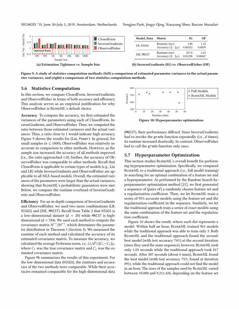
Figure 9: A study of statistics computationmethods: (left) a comparison of estimated parameter variances to the actual param-
eter variances, and (right) a comparison of two statistics computation methods.
5.6 Statistics Computation
In this section, we compare ClosedForm, InverseGradients,and ObservedFisher in terms of both accuracy and efficiency.This analysis serves as an empirical justification for whyObservedFisher is BlinkML’s default choice.
Accuracy To compare the accuracy, we first estimated thevariances of the parameters using each of ClosedForm, In-verseGradients, and ObservedFisher. Then, we computed theratio between those estimated variances and the actual vari-ances. Thus, a ratio close to 1 would indicate high accuracy.Figure 9 shows the results for (Lin, Power). In general, forsmall samples (n ≤ 1000), ObservedFisher was relatively in-accurate in comparison to other methods. However, as thesample size increased, the accuracy of all methods improved(i.e., the ratio approached 1.0); further, the accuracy of Ob-servedFisher was comparable to other methods. Recall thatClosedForm is applicable to certain types of models (e.g., Linand LR) while InverseGradients and ObservedFisher are ap-plicable to all MLE-based models. Overall, the estimated vari-ances of the parameters were larger than the actual variances,showing that BlinkML’s probabilistic guarantees were met.Below, we compare the runtime overhead of InverseGradi-ents and ObservedFisher.
Efficiency For an in-depth comparison of InverseGradientsand ObservedFisher, we used two more combinations (LR,HIGGS) and (ME, MNIST). Recall from Table 2 that HIGGS isa low-dimensional dataset (d = 28) while MNIST is high-dimensional (d = 784). We used each method to compute thecovariance matrix H−1 JH−1, which determines the parame-ter distribution in Theorem 1 (Section 3). We measured theruntime of each method and calculated the accuracy of itsestimated covariance matrix. To measure the accuracy, wecalculated the average Frobenius norm, i.e., (1/d2) ∥Ct−Ce ∥F ,where Ct was the true covariance matrix and Ce was the es-timated covariance matrix.Figure 9b summarizes the results of this experiment. For
the low-dimensional data (HIGGS), the runtimes and accura-cies of the two methods were comparable. While their accu-racies remained comparable for the high-dimensional data
0 10 20 30 40 50 6050%
60%
70%
80%
Runtime (min)
Accuracy
Full ModelsBlinkMLModels
Figure 10: Hyperparameter optimization
(MNIST), their performance differed. Since InverseGradientshad to invoke the grads function repeatedly (i.e., d times),its runtime increased drastically. In contrast, ObservedFisherhad to call the grads function only once.
5.7 Hyperparameter Optimization
This section studies BlinkML’s overall benefit for perform-ing hyperparameter optimization. Specifically, we comparedBlinkML to a traditional approach (i.e., full model training)in searching for an optimal combination of a feature set anda hyperparameter. As performed by the Random Search hy-perparameter optimization method [21], we first generateda sequence of (pairs of) a randomly chosen feature set anda regularization coefficient. Then, we let BlinkML train aseries of 95% accurate models using the feature set and theregularization coefficient in the sequence. Similarly, we letthe traditional approach train a series of exact models usingthe same combination of the feature set and the regulariza-tion coefficient.Figure 10 shows the result, where each dot represents a
model. Within half an hour, BlinkML trained 961 modelswhile the traditional approach was able to train only 3. BothBlinkML and the traditional approach found the second-best model (with test accuracy 74%) at the second iteration(since they used the same sequence); however, BlinkML tookonly 1.03 seconds while the traditional approach took 817seconds. After 387 seconds (about 6 mins), BlinkML foundthe best model (with test accuracy 75%; found at iteration#91), while the traditional approach could not find the modelin an hour. The sizes of the samples used by BlinkML variedbetween 10,000 and 9,211,426, depending on the feature set
BlinkML: Efficient Maximum Likelihood Estimation SIGMOD ’19, June 30-July 5, 2019, Amsterdam, Netherlands
010−
410−
310−
210−
1 10100K200K300K400K500K
Regularization Coefficient
Est.SampleSize
(a) Regularization
100 500 1K 5K 10K 50K100K
050K100K150K20K
Number of Params
Est.SampleSize
(b) Number of Params
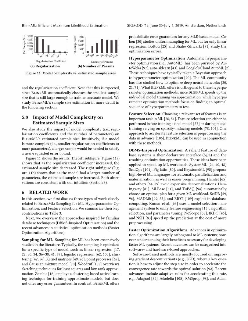
Figure 11: Model complexity vs. estimated sample sizes
and the regularization coefficient. Note that this is expected,since BlinkML automatically chooses the smallest samplesize that is still large enough to train an accurate model. Westudy BlinkML’s sample size estimation in more detail inthe following section.
5.8 Impact of Model Complexity on
Estimated Sample Sizes
We also study the impact of model complexity (i.e., regu-larization coefficients and the number of parameters) onBlinkML’s estimated sample size. Intuitively, if a modelis more complex (i.e., smaller regularization coefficients ormore parameters), a larger sample would be needed to satisfya user-requested error bound.
Figure 11 shows the results. The left subfigure (Figure 11a)shows that as the regularization coefficient increased, theestimated sample size decreased. The right subfigure (Fig-ure 11b) shows that as the model had a larger number ofparameters, the estimated sample size increased. Both obser-vations are consistent with our intuition (Section 3).
6 RELATEDWORK
In this section, we first discuss three types of work closelyrelated to BlinkML: Sampling for ML, Hyperparameter Op-timization, and Feature Selection. We summarize their keycontributions in Table 3.Next, we overview the approaches inspired by familiar
database techniques (DBMS-Inspired Optimization) and therecent advances in statistical optimization methods (FasterOptimization Algorithms).
Sampling for ML Sampling for ML has been extensivelystudied in the literature. Typically, the sampling is optimizedfor a specific type of model, such as linear regression [17,22, 30, 34, 36–38, 41, 47], logistic regression [62, 100], clus-tering [42, 56], Kernel matrices [49, 76], point processes [67],and Gaussian mixture model [70]. Woodruf [102] overviewssketching techniques for least squares and low rank approxi-mation. Zombie [16] employs a clustering-based active learn-ing technique for training approximate models, but doesnot offer any error guarantees. In contrast, BlinkML offers
probabilistic error guarantees for any MLE-based model. Co-hen [30] studies uniform sampling for ML, but for only linearregression. Bottou [25] and Shalev-Shwartz [91] study theoptimization errors.
Hyperparameter Optimization Automatic hyperparam-eter optimization (i.e., AutoML) has been pursued by Au-toWeka [97], auto-sklearn [43], andGoogle’s CloudAutoML [2].These techniques have typically taken a Bayesian approachto hyperparameter optimization [90]. The ML communityhas also studied how to optimize deep neural networks [20,21, 71]. What BlinkML offers is orthogonal to these hyperpa-rameter optimization methods, since BlinkML speeds up theindividual model training via approximation, while hyperpa-rameter optimization methods focus on finding an optimalsequence of hyperparameters to test.
Feature Selection Choosing a relevant set of features is animportant task in ML [26, 51]. Feature selection can either beperformed before training a final model [57] or during modeltraining relying on sparsity-inducing models [78, 104]. Oneapproach to accelerate feature selection is preprocessing thedata in advance [106]. BlinkML can be used in conjunctionwith these methods.
DBMS-Inspired Optimization A salient feature of data-base systems is their declarative interface (SQL) and theresulting optimization opportunities. These ideas have beenapplied to speed up ML workloads. SystemML [24, 40, 48]ScalOps [101], Pig latin [80], and KeystoneML [95] proposehigh-level ML languages for automatic parallelization andmaterialization, as well as easier programming. Hamlet [65]and others [64, 89] avoid expensive denormalizations. Hem-ingway [81], MLBase [61], and TuPAQ [94] automaticallychoose an optimal plan for a given ML workload. SciDB [59,96], MADLib [29, 55], and RIOT [109] exploit in-databasecomputing. Kumar et al. [63] uses a model selection man-agement system to unify feature engineering [15], algorithmselection, and parameter tuning. NoScope [58], tKDC [46],and NSH [83] speed up the prediction at the cost of morepreprocessing.
Faster Optimization Algorithms Advances in optimiza-tion algorithms are largely orthogonal to ML systems; how-ever, understanding their benefits is necessary for developingfaster ML systems. Recent advances can be categorized intosoftware- and hardware-based approaches.Software-based methods are mostly focused on improv-
ing gradient descent variants (e.g., SGD), where a key ques-tion is how to adjust the step size in order to accelerate theconvergence rate towards the optimal solution [92]. Recentadvances include adaptive rules for accelerating this rate,e.g., Adagrad [39], Adadelta [105], RMSprop [98], and Adam
SIGMOD ’19, June 30-July 5, 2019, Amsterdam, Netherlands Yongjoo Park, Jingyi Qing, Xiaoyang Shen, Barzan Mozafari
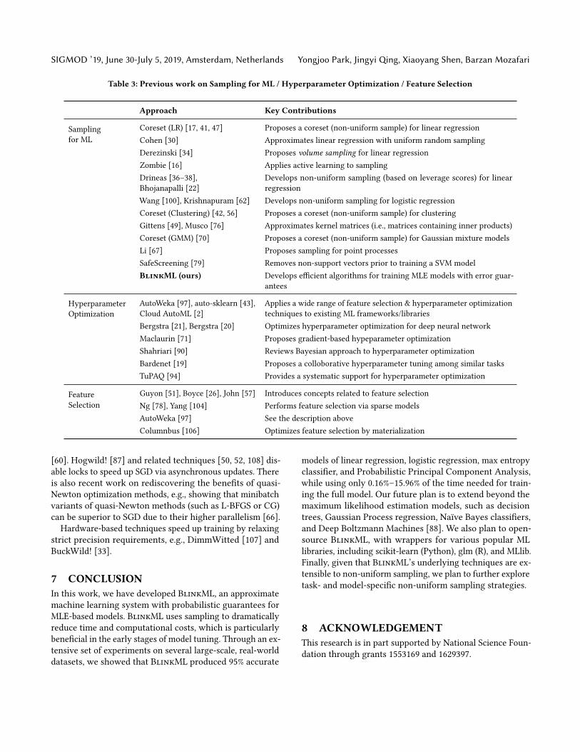
Table 3: Previous work on Sampling for ML / Hyperparameter Optimization / Feature Selection
Approach Key Contributions
Samplingfor ML
Coreset (LR) [17, 41, 47] Proposes a coreset (non-uniform sample) for linear regressionCohen [30] Approximates linear regression with uniform random samplingDerezinski [34] Proposes volume sampling for linear regressionZombie [16] Applies active learning to samplingDrineas [36–38],Bhojanapalli [22]
Develops non-uniform sampling (based on leverage scores) for linearregression
Wang [100], Krishnapuram [62] Develops non-uniform sampling for logistic regressionCoreset (Clustering) [42, 56] Proposes a coreset (non-uniform sample) for clusteringGittens [49], Musco [76] Approximates kernel matrices (i.e., matrices containing inner products)Coreset (GMM) [70] Proposes a coreset (non-uniform sample) for Gaussian mixture modelsLi [67] Proposes sampling for point processesSafeScreening [79] Removes non-support vectors prior to training a SVM modelBlinkML (ours) Develops efficient algorithms for training MLE models with error guar-
antees
HyperparameterOptimization
AutoWeka [97], auto-sklearn [43],Cloud AutoML [2]
Applies a wide range of feature selection & hyperparameter optimizationtechniques to existing ML frameworks/libraries
Bergstra [21], Bergstra [20] Optimizes hyperparameter optimization for deep neural networkMaclaurin [71] Proposes gradient-based hypeparameter optimizationShahriari [90] Reviews Bayesian approach to hyperparameter optimizationBardenet [19] Proposes a colloborative hyperparameter tuning among similar tasksTuPAQ [94] Provides a systematic support for hyperparameter optimization
FeatureSelection
Guyon [51], Boyce [26], John [57] Introduces concepts related to feature selectionNg [78], Yang [104] Performs feature selection via sparse modelsAutoWeka [97] See the description aboveColumnbus [106] Optimizes feature selection by materialization
[60]. Hogwild! [87] and related techniques [50, 52, 108] dis-able locks to speed up SGD via asynchronous updates. Thereis also recent work on rediscovering the benefits of quasi-Newton optimization methods, e.g., showing that minibatchvariants of quasi-Newton methods (such as L-BFGS or CG)can be superior to SGD due to their higher parallelism [66].
Hardware-based techniques speed up training by relaxingstrict precision requirements, e.g., DimmWitted [107] andBuckWild! [33].
7 CONCLUSION
In this work, we have developed BlinkML, an approximatemachine learning system with probabilistic guarantees forMLE-based models. BlinkML uses sampling to dramaticallyreduce time and computational costs, which is particularlybeneficial in the early stages of model tuning. Through an ex-tensive set of experiments on several large-scale, real-worlddatasets, we showed that BlinkML produced 95% accurate
models of linear regression, logistic regression, max entropyclassifier, and Probabilistic Principal Component Analysis,while using only 0.16%–15.96% of the time needed for train-ing the full model. Our future plan is to extend beyond themaximum likelihood estimation models, such as decisiontrees, Gaussian Process regression, Naïve Bayes classifiers,and Deep Boltzmann Machines [88]. We also plan to open-source BlinkML, with wrappers for various popular MLlibraries, including scikit-learn (Python), glm (R), and MLlib.Finally, given that BlinkML’s underlying techniques are ex-tensible to non-uniform sampling, we plan to further exploretask- and model-specific non-uniform sampling strategies.
8 ACKNOWLEDGEMENT
This research is in part supported by National Science Foun-dation through grants 1553169 and 1629397.
BlinkML: Efficient Maximum Likelihood Estimation SIGMOD ’19, June 30-July 5, 2019, Amsterdam, Netherlands
REFERENCES
[1] Apache spark’s scalable machine learning library. https://spark.apache.org/mllib/. Retrieved: July 18, 2018.
[2] Cloud automl. https://cloud.google.com/automl/. Retrieved: Oct 30, 2018.[3] Conda. https://conda.io/docs/index.html. Retrieved: July 18, 2018.[4] cx_oracle version 6.2. https://oracle.github.io/python-cx_Oracle/. Retrieved:
July 18, 2018.[5] Download kaggle display advertising challenge dataset. http://labs.criteo.com/
2014/02/download-kaggle-display-advertising-challenge-dataset/. Retrieved:Oct 30, 2018.
[6] ibmdbr: Ibm in-database analytics for r. https://cran.r-project.org/web/packages/ibmdbR/index.html. Retrieved: July 18, 2018.
[7] Individual household electric power consumption data set. https://archive.ics.uci.edu/ml/datasets/Individual+household+electric+power+consumption. Re-trieved: Oct 30, 2018.
[8] The infinite mnist dataset. http://leon.bottou.org/projects/infimnist. Retrieved:July 18, 2018.
[9] Python sql driver - pymssql. https://docs.microsoft.com/en-us/sql/connect/python/pymssql/python-sql-driver-pymssql. Retrieved: July 18, 2018.
[10] Python support for ibm db2 and ibm informix. https://github.com/ibmdb/python-ibmdb. Retrieved: July 18, 2018.
[11] R interface to oracle data mining. http://www.oracle.com/technetwork/database/options/odm/odm-r-integration-089013.html. Retrieved: July 18,2018.
[12] Revoscaler. https://docs.microsoft.com/en-us/sql/advanced-analytics/r/revoscaler-overview. Retrieved: July 18, 2018.
[13] Yelp dataset. https://www.kaggle.com/yelp-dataset/yelp-dataset. Retrieved:July 18, 2018.
[14] S. Agarwal, H. Milner, A. Kleiner, A. Talwalkar, M. Jordan, S. Madden, B. Moza-fari, and I. Stoica. Knowing when you’re wrong: Building fast and reliableapproximate query processing systems. In SIGMOD, 2014.
[15] M. R. Anderson, D. Antenucci, V. Bittorf, M. Burgess, M. J. Cafarella, A. Kumar,F. Niu, Y. Park, C. Ré, and C. Zhang. Brainwash: A data system for featureengineering. In CIDR, 2013.
[16] M. R. Anderson and M. Cafarella. Input selection for fast feature engineering.In ICDE, pages 577–588, 2016.
[17] O. Bachem, M. Lucic, and A. Krause. Practical coreset constructions for ma-chine learning. arXiv preprint arXiv:1703.06476, 2017.
[18] P. Baldi, P. Sadowski, and D. Whiteson. Searching for exotic particles in high-energy physics with deep learning. Nature communications, 2014.
[19] R. Bardenet, M. Brendel, B. Kégl, and M. Sebag. Collaborative hyperparametertuning. In ICML, 2013.
[20] J. Bergstra, D. Yamins, and D. D. Cox. Making a science of model search: Hy-perparameter optimization in hundreds of dimensions for vision architectures.2013.
[21] J. S. Bergstra, R. Bardenet, Y. Bengio, and B. Kégl. Algorithms for hyper-parameter optimization. In NIPS, 2011.
[22] S. Bhojanapalli, P. Jain, and S. Sanghavi. Tighter low-rank approximation viasampling the leveraged element. In SODA, 2015.
[23] C. M. Bishop. Pattern recognition and machine learning. 2006.[24] M. Boehm, M. W. Dusenberry, D. Eriksson, A. V. Evfimievski, F. M. Manshadi,
N. Pansare, B. Reinwald, F. R. Reiss, P. Sen, A. C. Surve, et al. Systemml: Declar-ative machine learning on spark. PVLDB, pages 1425–1436, 2016.
[25] L. Bottou and O. Bousquet. The tradeoffs of large scale learning. In NIPS, 2008.[26] D. Boyce, A. Farhi, and R. Weischedel. Optimal subset selection: Multiple regres-
sion, interdependence and optimal network algorithms. 2013.[27] K. Chakrabarti, M. N. Garofalakis, R. Rastogi, and K. Shim. Approximate query
processing using wavelets. In VLDB, September 2000.[28] B.-Y. Chu, C.-H. Ho, C.-H. Tsai, C.-Y. Lin, and C.-J. Lin. Warm start for param-
eter selection of linear classifiers. In KDD, 2015.[29] J. Cohen, B. Dolan, M. Dunlap, J. M. Hellerstein, and C.Welton. Mad skills: new
analysis practices for big data. PVLDB, pages 1481–1492, 2009.[30] M. B. Cohen, Y. T. Lee, C. Musco, C. Musco, R. Peng, and A. Sidford. Uniform
sampling for matrix approximation. In ITCS, 2015.[31] D. Crankshaw, X. Wang, G. Zhou, M. J. Franklin, J. E. Gonzalez, and I. Stoica.
Clipper: A low-latency online prediction serving system. In NSDI, pages 613–627, 2017.
[32] A. Crotty, A. Galakatos, E. Zgraggen, C. Binnig, and T. Kraska. Vizdom: Inter-active analytics through pen and touch. PVLDB, pages 2024–2027, 2015.
[33] C. De Sa, M. Feldman, C. Ré, and K. Olukotun. Understanding and optimizingasynchronous low-precision stochastic gradient descent. In Proceedings of the
44th Annual International Symposium on Computer Architecture, pages 561–574.ACM, 2017.
[34] M. Derezinski and M. K. Warmuth. Unbiased estimates for linear regressionvia volume sampling. In NIPS, 2017.
[35] A. Dobra, C. Jermaine, F. Rusu, and F. Xu. Turbo-charging estimate conver-gence in dbo. PVLDB, 2009.
[36] P. Drineas, M. Magdon-Ismail, M. W. Mahoney, and D. P. Woodruff. Fast ap-proximation of matrix coherence and statistical leverage. JMLR, 2012.
[37] P. Drineas, M. W. Mahoney, and S. Muthukrishnan. Sampling algorithms for l2 regression and applications. In SODA, 2006.
[38] P. Drineas, M. W. Mahoney, S. Muthukrishnan, and T. Sarlós. Faster leastsquares approximation. Numerische mathematik, 2011.
[39] J. Duchi, E. Hazan, and Y. Singer. Adaptive subgradient methods for onlinelearning and stochastic optimization. Journal of Machine Learning Research,12(Jul):2121–2159, 2011.
[40] A. Elgohary, M. Boehm, P. J. Haas, F. R. Reiss, and B. Reinwald. Compressedlinear algebra for large-scale machine learning. PVLDB, pages 960–971, 2016.
[41] D. Feldman and M. Langberg. A unified framework for approximating andclustering data. In STOC, 2011.
[42] D. Feldman, M. Schmidt, and C. Sohler. Turning big data into tiny data:Constant-size coresets for k-means, pca and projective clustering. In SODA,2013.
[43] M. Feurer, A. Klein, K. Eggensperger, J. Springenberg, M. Blum, and F. Hutter.Efficient and robust automated machine learning. In NIPS, 2015.
[44] J. Fonollosa, S. Sheik, R. Huerta, and S. Marco. Reservoir computing compen-sates slow response of chemosensor arrays exposed to fast varying gas concen-trations in continuous monitoring. Sensors and Actuators B: Chemical, 2015.
[45] A. Galakatos, A. Crotty, E. Zgraggen, C. Binnig, and T. Kraska. Revisiting reusefor approximate query processing. PVLDB, pages 1142–1153, 2017.
[46] E. Gan and P. Bailis. Scalable kernel density classification via threshold-basedpruning. In SIGMOD, pages 945–959, 2017.
[47] M. Ghashami and J. M. Phillips. Relative errors for deterministic low-rank ma-trix approximations. In SODA, 2014.
[48] A. Ghoting, R. Krishnamurthy, E. Pednault, B. Reinwald, V. Sindhwani,S. Tatikonda, Y. Tian, and S. Vaithyanathan. Systemml: Declarative machinelearning on mapreduce. In ICDE, pages 231–242, 2011.
[49] A. Gittens and M. W. Mahoney. Revisiting the nyström method for improvedlarge-scale machine learning. JMLR, 2016.
[50] J. E. Gonzalez, P. Bailis, M. I. Jordan, M. J. Franklin, J. M. Hellerstein, A. Gh-odsi, and I. Stoica. Asynchronous complex analytics in a distributed dataflowarchitecture. arXiv preprint arXiv:1510.07092, 2015.
[51] I. Guyon and A. Elisseeff. An introduction to variable and feature selection.The Journal of Machine Learning Research, 3:1157–1182, 2003.
[52] S. Hadjis, C. Zhang, I. Mitliagkas, D. Iter, and C. Ré. Omnivore: An optimizer formulti-device deep learning on cpus and gpus. arXiv preprint arXiv:1606.04487,2016.
[53] M. Hall, E. Frank, G. Holmes, B. Pfahringer, P. Reutemann, and I. H. Witten.The WEKA data mining software: an update. SIGKDD Explorations, 2009.
[54] W. He, Y. Park, I. Hanafi, J. Yatvitskiy, and B. Mozafari. Demonstration of ver-dictdb, the platform-independent aqp system. In SIGMOD, 2018.
[55] J. M. Hellerstein, C. Ré, F. Schoppmann, D. Z. Wang, E. Fratkin, A. Gorajek, K. S.Ng, C. Welton, X. Feng, K. Li, et al. The madlib analytics library: or mad skills,the sql. PVLDB, pages 1700–1711, 2012.
[56] R. Jaiswal, A. Kumar, and S. Sen. A simple d 2-sampling based ptas for k-meansand other clustering problems. 2014.
[57] G. H. John, R. Kohavi, and K. Pfleger. Irrelevant features and the subset selectionproblem. In Machine Learning Proceedings. 1994.
[58] D. Kang, J. Emmons, F. Abuzaid, P. Bailis, and M. Zaharia. Noscope: optimizingneural network queries over video at scale. PVLDB, pages 1586–1597, 2017.
[59] M. Kersten, Y. Zhang, M. Ivanova, and N. Nes. Sciql, a query language forscience applications. In Proceedings of the EDBT/ICDT 2011 Workshop on Array
Databases, pages 1–12, 2011.[60] D. Kingma and J. Ba. Adam: A method for stochastic optimization. arXiv
preprint arXiv:1412.6980, 2014.[61] T. Kraska, A. Talwalkar, J. C. Duchi, R. Griffith, M. J. Franklin, and M. I. Jordan.
Mlbase: A distributed machine-learning system. In CIDR, 2013.[62] B. Krishnapuram, L. Carin, M. A. Figueiredo, and A. J. Hartemink. Sparse multi-
nomial logistic regression: Fast algorithms and generalization bounds. TPAMI,2005.
[63] A. Kumar, R. McCann, J. Naughton, and J. M. Patel. Model selection manage-ment systems: The next frontier of advanced analytics. SIGMOD Record, pages17–22, 2016.
[64] A. Kumar, J. Naughton, and J. M. Patel. Learning generalized linear modelsover normalized data. In SIGMOD, pages 1969–1984, 2015.
[65] A. Kumar, J. Naughton, J. M. Patel, and X. Zhu. To join or not to join?: Thinkingtwice about joins before feature selection. In Proceedings of the 2016 Interna-
tional Conference on Management of Data, pages 19–34. ACM, 2016.[66] Q. V. Le, J. Ngiam, A. Coates, A. Lahiri, B. Prochnow, and A. Y. Ng. On opti-
mization methods for deep learning. In ICML, pages 265–272, 2011.[67] C. Li, S. Jegelka, and S. Sra. Efficient sampling for k-determinantal point pro-
cesses. arXiv preprint arXiv:1509.01618, 2015.[68] F. Li, B. Wu, K. Yi, and Z. Zhao. Wander join: Online aggregation via random
walks. In Proceedings of the 2016 International Conference on Management of
SIGMOD ’19, June 30-July 5, 2019, Amsterdam, Netherlands Yongjoo Park, Jingyi Qing, Xiaoyang Shen, Barzan Mozafari
Data, SIGMOD Conference 2016, San Francisco, CA, USA, June 26 - July 01, 2016,2016.
[69] C.-J. Lin, R. C. Weng, and S. S. Keerthi. Trust region newton method for logisticregression. JMLR, 2008.
[70] M. Lucic, M. Faulkner, A. Krause, and D. Feldman. Training gaussian mixturemodels at scale via coresets. JMLR, 2017.
[71] D. Maclaurin, D. Duvenaud, and R. Adams. Gradient-based hyperparameteroptimization through reversible learning. In ICML, 2015.
[72] J. Martens. Deep learning via hessian-free optimization. In ICML, 2010.[73] S. Melnik, A. Gubarev, J. J. Long, G. Romer, S. Shivakumar, M. Tolton, and T. Vas-
silakis. Dremel: interactive analysis of web-scale datasets. Commun. ACM, 54,2011.
[74] M. Mohri, A. Rostamizadeh, and A. Talwalkar. Foundations of machine learning.MIT press, 2012.
[75] B. Mozafari and N. Niu. A handbook for building an approximate query engine.IEEE Data Eng. Bull., 2015.
[76] C. Musco and C. Musco. Recursive sampling for the nystrom method. In NIPS,2017.
[77] W. K. Newey andD.McFadden. Large sample estimation and hypothesis testing.Handbook of econometrics, pages 2111–2245, 1994.
[78] A. Y. Ng. Feature selection, l 1 vs. l 2 regularization, and rotational invariance.In ICML, 2004.
[79] K. Ogawa, Y. Suzuki, and I. Takeuchi. Safe screening of non-support vectors inpathwise svm computation. In ICML, 2013.
[80] C. Olston, B. Reed, U. Srivastava, R. Kumar, and A. Tomkins. Pig latin: a not-so-foreign language for data processing. In SIGMOD, pages 1099–1110, 2008.
[81] X. Pan, S. Venkataraman, Z. Tai, and J. Gonzalez. Hemingway: modeling dis-tributed optimization algorithms. arXiv, 2017.
[82] N. Pansare, V. R. Borkar, C. Jermaine, and T. Condie. Online aggregation forlarge mapreduce jobs. PVLDB, 4, 2011.
[83] Y. Park, M. Cafarella, and B. Mozafari. Neighbor-sensitive hashing. PVLDB,2015.
[84] Y. Park, B. Mozafari, J. Sorenson, and J. Wang. Verdictdb: universalizing ap-proximate query processing. In SIGMOD, 2018.
[85] Y. Park, A. S. Tajik, M. Cafarella, and B. Mozafari. Database Learning: Towardsa database that becomes smarter every time. In SIGMOD, 2017.
[86] F. Pedregosa, G. Varoquaux, A. Gramfort, V. Michel, B. Thirion, O. Grisel,M. Blondel, P. Prettenhofer, R. Weiss, V. Dubourg, J. Vanderplas, A. Passos,D. Cournapeau, M. Brucher, M. Perrot, and E. Duchesnay. Scikit-learn: Ma-chine learning in Python. JMLR, 2011.
[87] B. Recht, C. Re, S. Wright, and F. Niu. Hogwild: A lock-free approach to paral-lelizing stochastic gradient descent. In NIPS, pages 693–701, 2011.
[88] R. Salakhutdinov and H. Larochelle. Efficient learning of deep boltzmann ma-chines. In AISTATS, 2010.
[89] M. Schleich, D. Olteanu, and R. Ciucanu. Learning linear regression modelsover factorized joins. In SIGMOD, pages 3–18, 2016.
[90] B. Shahriari, K. Swersky, Z. Wang, R. P. Adams, and N. De Freitas. Taking thehuman out of the loop: A review of bayesian optimization. Proceedings of theIEEE, 2016.
[91] S. Shalev-Shwartz and N. Srebro. Svm optimization: inverse dependence ontraining set size. In ICML, 2008.
[92] C. J. Shallue, J. Lee, J. Antognini, J. Sohl-Dickstein, R. Frostig, and G. E. Dahl.Measuring the effects of data parallelism on neural network training. 2018.
[93] J. Shin, S. Wu, F. Wang, C. De Sa, C. Zhang, and C. Ré. Incremental knowledgebase construction using deepdive. PVLDB, pages 1310–1321, 2015.
[94] E. R. Sparks, A. Talwalkar, D. Haas, M. J. Franklin, M. I. Jordan, and T. Kraska.Automating model search for large scale machine learning. In SoCC, pages368–380, 2015.
[95] E. R. Sparks, S. Venkataraman, T. Kaftan, M. J. Franklin, and B. Recht. Key-stoneML: Optimizing pipelines for large-scale advanced analytics. In ICDE,pages 535–546, 2017.
[96] M. Stonebraker, P. Brown, D. Zhang, and J. Becla. Scidb: A database manage-ment system for applications with complex analytics. Computing in Science &
Engineering, pages 54–62, 2013.[97] C. Thornton, F. Hutter, H. H. Hoos, and K. Leyton-Brown. Auto-weka: Com-
bined selection and hyperparameter optimization of classification algorithms.In KDD, 2013.
[98] T. Tieleman and G. Hinton. Lecture 6.5-rmsprop, coursera: Neural networksfor machine learning. University of Toronto, Tech. Rep, 2012.
[99] M. E. Tipping and C. M. Bishop. Probabilistic principal component analysis.Journal of the Royal Statistical Society: Series B (Statistical Methodology), 1999.
[100] H. Wang, R. Zhu, and P. Ma. Optimal subsampling for large sample logisticregression. JASA, 2018.
[101] M. Weimer, T. Condie, R. Ramakrishnan, et al. Machine learning in scalops, ahigher order cloud computing language. In BigLearn, pages 389–396, 2011.
[102] D. P. Woodruff et al. Sketching as a tool for numerical linear algebra. FnT-TCS,2014.
[103] E. Xing. Vc dimension and model complexity. https://www.cs.cmu.edu/~epxing/Class/10701/slides/lecture16-VC.pdf. Retrieved: July 18, 2018.
[104] A. Y. Yang, J. Wright, Y. Ma, and S. S. Sastry. Feature selection in face recogni-tion: A sparse representation perspective. TPAML, 2007.
[105] M. D. Zeiler. Adadelta: an adaptive learning rate method. arXiv preprint
arXiv:1212.5701, 2012.[106] C. Zhang, A. Kumar, and C. Ré. Materialization optimizations for feature selec-
tion workloads. In SIGMOD, pages 265–276, 2014.[107] C. Zhang and C. Ré. Dimmwitted: A study of main-memory statistical analytics.
Proceedings of the VLDB Endowment, 7(12):1283–1294, 2014.[108] S. Zhang, C. Zhang, Z. You, R. Zheng, and B. Xu. Asynchronous stochastic
gradient descent for dnn training. In Acoustics, Speech and Signal Processing
(ICASSP), 2013 IEEE International Conference on, pages 6660–6663. IEEE, 2013.[109] Y. Zhang, W. Zhang, and J. Yang. I/o-efficient statistical computing with riot.
In ICDE, pages 1157–1160, 2010.
A MODEL ABSTRACTION EXAMPLES
This section shows that BlinkML-supported ML models canbe cast into the abstract form in Equation (2). For illustration,we use logistic regression and PPCA.
Logistic Regression The objective function of logistic re-gression captures the difference between true class labelsand the predicted class labels. An optional regularizationterm may be placed to prevent a model from being overfit-ted to a training set. For instance, the objective function ofL2-regularized logistic regression is expressed as follows:
fn(θ ) = −
[1n
n∑i=1
ti logσ (θ⊤xi ) + (1 − ti ) logσ (1 − θ⊤xi )
]+β
2∥θ ∥2
where σ (y) = 1/(1 + exp(y)) is a sigmoid function, and β isthe coefficient that controls the strength of the regularizationpenalty. The observed class labels, i.e., ti for i = 1, . . . ,n, areeither 0 or 1. The above expression is minimized when θ is setto the value at which the gradient ∇fn(θ ) of fn(θ ) becomesa zero vector; that is,
∇fn(θ ) =
[1n
n∑i=1
(σ (θ⊤xi ) − ti )xi
]+ β θ = 0
It is straightforward to cast the above expression into Equa-tion (3). That is, q(θ ;xi , ti ) = (σ (θ⊤xi )− ti )xi and r (θ ) = β θ .
PPCA The objective function of PPCA captures the differ-ence between the covariance matrix S of the training set andthe covariance matrix C = ΘΘ⊤ + σ 2I reconstructed fromthe q number of extracted factors Θ, as follows:
fn(Θ) =12
(d log 2π + log |C | + tr(C−1S)
)where d is the dimension of feature vectors. Θ is a d-by-qmatrix in which each column represents a factor, and σ isa real-valued scalar that represents the noise in data notexplained by those factors. The optimal value for σ can beobtained once the values for Θ are determined. The value ofq, or the number of the factors to extract, is a user parameter.The above expression fn(Θ) is minimized when its gradient
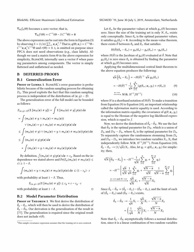
BlinkML: Efficient Maximum Likelihood Estimation SIGMOD ’19, June 30-July 5, 2019, Amsterdam, Netherlands
∇Θ fn(Θ) becomes a zero vector; that is,
∇Θ f (Θ) = C−1(Θ − S C−1Θ) = 0
The above expression can be cast into the form in Equation (3)by observing S = (1/n)
∑ni=1 xix
⊤i .
5 That is,q(Θ;xi ) = C−1Θ−C−1xix⊤
i C−1Θ and r (Θ) = 0. ti is omitted on purpose since
PPCA does not need observations (e.g., class labels). Al-though we used a matrix form Θ in the above expression forsimplicity, BlinkML internally uses a vector θ when pass-ing parameters among components. The vector is simplyflattened and unflattened as needed.
B DEFERRED PROOFS
B.1 Generalization Error
Proof of Lemma 1. BlinkML’s error guarantee is proba-bilistic because of the random sampling process for obtainingDn . This proof exploits the fact that this random samplingprocess is independent of the distribution of (x ,y) ∼ D.
The generalization error of the full model can be boundedas follows:
E(x ,y)∼D(1 [mN (x) , y]) =
∫1 [mN (x) , y] p(x)dx
=
∫(mn(x) , y ∧mn(x) =mN (x))
∨ (mn(x) = y ∧mn(x) ,mN (x))p(x)dx
≤
∫(mn(x) , y) ∨ (mn(x) = y ∧mn(x) ,mN (x))p(x)dx
≤
∫(mn(x) , y)p(x)dx
+
∫(mn(x) = y ∧mn(x) ,mN (x))p(x)dx
By definition,∫(mn(x) , y)p(x)dx = εд . Based on the in-
dependence we stated above and Pr(Ex (mn(x) ,mN (x)) ≤ε) ≥ 1 − δ ,∫
(mn(x) = y ∧mn(x) ,mN (x))p(x)dx ≤ (1 − εд) · ε
with probability at least 1 − δ . Thus,
E(x ,y)∼D(1 [mN (x) , y]) ≤ εд + ε − εд · ε
with probability at least 1 − δ .
B.2 Model Parameter Distribution
Proof of Theorem 1. We first derive the distribution ofθn −θ∞, which will then be used to derive the distribution ofθn − θN . Our derivation is the generalization of the result in[77]. The generalization is required since the original resultdoes not include r (θ ).
5This sample covariance expression assumes that the training set is zero-centered.
Let θ∞ be the parameter values at which д∞(θ ) becomeszero. Since the size of the training set is only N , θ∞ existsonly conceptually. Since θn is the optimal parameter values,it satisfies дn(θn) = 0. According to the mean-value theorem,there exists θ between θn and θ∞ that satisfies:
H (θ )(θn − θ∞) = дn(θn) − дn(θ∞) = −дn(θ∞)
where H (θ ) is the Jacobian of дn(θ ) evaluated at θ . Note thatдn(θn) is zero since θn is obtained by finding the parameterat which дn(θ ) becomes zero.Applying the multidimensional central limit theorem to
the above equation produces the following:√n
(θn − θ∞
)= −H (θ )−1 √n дn(θ∞)
= −H (θ )−1 1√n
n∑i=1
(q(θ∞;xi ,yi ) + r (θ∞)) (9)
n→∞−−−−→ N(0, H−1 JH−1) (10)
whereH is a shorthand notation ofH (θ ). Tomake a transitionfrom Equation (9) to Equation (10), an important relationshipcalled the information matrix equality is used. According tothe information matrix equality, the covariance of q(θ ;xi ,yi )is equal to the Hessian of the negative log-likelihood expres-sion, which is equal to J .
Now, we derive the distribution of θn − θN . We use the factthat θN is the optimal parameter for DN , which is a union ofDn and DN − Dn , where θn is the optimal parameter for Dn .To separately capture the randomness stemming from DnandDN −Dn , we introduce two random variablesX1,X2 thatindependently follow N(0, H−1 JH−1). From Equation (10),θn − θ∞ → (1/
√n)X1. Also, let qi = q(θ∞;xi ,yi ) for simplic-
ity; then,
√N
(θN − θ∞
)= −H−1 1
√N(
n∑i=1
qi +N−n∑i=1
qi )
= −H−1
[ √n
√N
1√n
n∑i=1
qi +
√N − n√N
1√N − n
N−n∑i=1
qi
]n→∞ and N→∞−−−−−−−−−−−−−→
√n
√NX1 +
√N − n√N
X2
Since θn − θN = (θn − θ∞) − (θN − θ∞), and the limit of eachof (θn − θ∞) and (θN − θ∞) exists,
θn − θN →1√nX1 −
√n
NX1 −
√N − n
NX2
=
(1√n−
√n
N
)X1 −
√N − n
NX2
Note that θn − θN asymptotically follows a normal distribu-tion, since it is a linear combination of two random variables
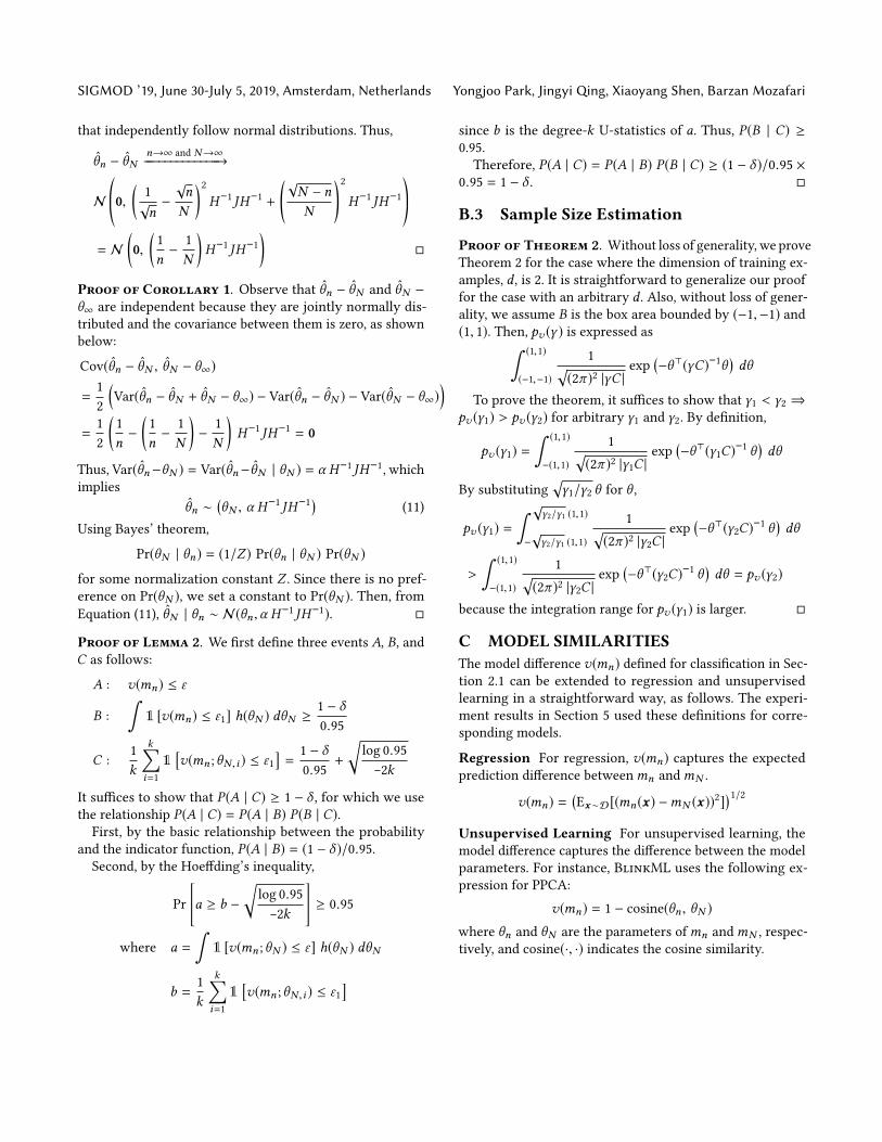
SIGMOD ’19, June 30-July 5, 2019, Amsterdam, Netherlands Yongjoo Park, Jingyi Qing, Xiaoyang Shen, Barzan Mozafari
that independently follow normal distributions. Thus,
θn − θNn→∞ and N→∞−−−−−−−−−−−−−→
N©«0,
(1√n−
√n
N
)2
H−1 JH−1 +
(√N − n
N
)2
H−1 JH−1ª®¬= N
(0,
(1n−
1N
)H−1 JH−1
)
Proof of Corollary 1. Observe that θn − θN and θN −
θ∞ are independent because they are jointly normally dis-tributed and the covariance between them is zero, as shownbelow:
Cov(θn − θN , θN − θ∞)
=12
(Var(θn − θN + θN − θ∞) − Var(θn − θN ) − Var(θN − θ∞)
)=
12
(1n−
(1n−
1N
)−
1N
)H−1 JH−1 = 0
Thus, Var(θn−θN ) = Var(θn−θN | θN ) = α H−1 JH−1, whichimplies
θn ∼(θN , α H−1 JH−1) (11)
Using Bayes’ theorem,
Pr(θN | θn) = (1/Z ) Pr(θn | θN ) Pr(θN )
for some normalization constant Z . Since there is no pref-erence on Pr(θN ), we set a constant to Pr(θN ). Then, fromEquation (11), θN | θn ∼ N(θn ,α H−1 JH−1).
Proof of Lemma 2. We first define three events A, B, andC as follows:
A : v(mn) ≤ ε
B :∫
1 [v(mn) ≤ ε1] h(θN ) dθN ≥1 − δ
0.95
C :1k
k∑i=1
1[v(mn ;θN ,i ) ≤ ε1
]=
1 − δ
0.95+
√log 0.95
−2k
It suffices to show that P(A | C) ≥ 1 − δ , for which we usethe relationship P(A | C) = P(A | B) P(B | C).First, by the basic relationship between the probability
and the indicator function, P(A | B) = (1 − δ )/0.95.Second, by the Hoeffding’s inequality,
Pr
[a ≥ b −
√log 0.95
−2k
]≥ 0.95
where a =
∫1 [v(mn ;θN ) ≤ ε] h(θN ) dθN
b =1k
k∑i=1
1[v(mn ;θN ,i ) ≤ ε1
]
since b is the degree-k U-statistics of a. Thus, P(B | C) ≥
0.95.Therefore, P(A | C) = P(A | B) P(B | C) ≥ (1 − δ )/0.95 ×
0.95 = 1 − δ .
B.3 Sample Size Estimation
Proof of Theorem 2. Without loss of generality, we proveTheorem 2 for the case where the dimension of training ex-amples, d , is 2. It is straightforward to generalize our prooffor the case with an arbitrary d . Also, without loss of gener-ality, we assume B is the box area bounded by (−1,−1) and(1, 1). Then, pv (γ ) is expressed as∫ (1,1)
(−1,−1)
1√(2π )2 |γC |
exp(−θ⊤(γC)−1θ
)dθ
To prove the theorem, it suffices to show that γ1 < γ2 ⇒
pv (γ1) > pv (γ2) for arbitrary γ1 and γ2. By definition,
pv (γ1) =
∫ (1,1)
−(1,1)
1√(2π )2 |γ1C |
exp(−θ⊤(γ1C)
−1 θ)dθ
By substituting√γ1/γ2 θ for θ ,
pv (γ1) =
∫ √γ2/γ1 (1,1)
−√γ2/γ1 (1,1)
1√(2π )2 |γ2C |
exp(−θ⊤(γ2C)
−1 θ)dθ
>
∫ (1,1)
−(1,1)
1√(2π )2 |γ2C |
exp(−θ⊤(γ2C)
−1 θ)dθ = pv (γ2)
because the integration range for pv (γ1) is larger.
C MODEL SIMILARITIES
The model difference v(mn) defined for classification in Sec-tion 2.1 can be extended to regression and unsupervisedlearning in a straightforward way, as follows. The experi-ment results in Section 5 used these definitions for corre-sponding models.
Regression For regression, v(mn) captures the expectedprediction difference betweenmn andmN .
v(mn) =(Ex∼D[(mn(x) −mN (x))
2])1/2
Unsupervised Learning For unsupervised learning, themodel difference captures the difference between the modelparameters. For instance, BlinkML uses the following ex-pression for PPCA:
v(mn) = 1 − cosine(θn , θN )where θn and θN are the parameters ofmn andmN , respec-tively, and cosine(·, ·) indicates the cosine similarity.