Embed Size (px)
Citation preview

Sains Malaysiana 45(6)(2016): 989–998
Block Backward Differentiation Formulas for Solving First Order Fuzzy Differential Equations under Generalized Differentiability
( Formula Blok Pembezaan Kebelakang bagi Menyelesaikan Persamaan Pembezaan Kabur Peringkat Pertama di bawah Kebolehbezaan Umum)
ISKANDAR SHAH MOHD ZAWAWI & ZARINA BIBI IBRAHIM*
ABSTRACT
In this paper, the fully implicit 2-point block backward differentiation formula and diagonally implicit 2-point block backward differentiation formula were developed under the interpretation of generalized differentiability concept for solving first order fuzzy differential equations. Some fuzzy initial value problems were tested in order to demonstrate the performance of the developed methods. The approximated solutions for both methods were in good agreement with the exact solutions. The numerical results showed that the diagonally implicit method outperforms the fully implicit method in term of accuracy.
Keywords: Block; diagonally; fuzzy; implicit
ABSTRAK
Dalam kertas ini, formula 2-titik blok pembezaan kebelakang tersirat penuh dan formula 2-titik blok pembezaan kebelakang tersirat pepenjuru dibangunkan di bawah konsep kebolehbezaan umum bagi menyelesaikan persamaan pembezaan kabur peringkat pertama. Beberapa masalah-masalah nilai awal kabur diuji untuk menunjukkan prestasi kaedah yang dibangunkan. Penyelesaian yang dianggarkan bagi kedua-dua kaedah adalah dalam persetujuan yang baik dengan penyelesaian tepat. Keputusan berangka menunjukkan kaedah tersirat pepenjuru mengatasi kaedah tersirat penuh dalam terma kejituan.
Kata kunci: Blok; kabur; pepenjuru; tersirat
INTRODUCTION
Differential equations with uncertainty plays serve as mathematical models in many fields such as science, physics, economics, psychology, defense and demography. This type of differential equations is called fuzzy differential equations (FDEs). There are different approaches to deal with FDEs. The first and most popular approach is using H-derivative or its generalization, the Hukuhara differentiability which is introduced by Puri and Ralescu (1983). However this approach suffers certain disadvantage that it leads to solutions with increasing support since the diameter of the solution is unbounded as time increases (Chalco-Cano & Roman-Flores 2008). In this direction, Bede and Gal (2005) introduced the generalized differentiability in order to resolve the above mentioned by enlarging the class of fuzzy valued function. In addition, Bede et al. (2007) stated that under certain appropriate conditions, FDEs is equivalent to a system of ordinary differential equations (ODEs) which can be solved by any suitable numerical method. The development of numerical methods for solving FDEs has been presented by many researchers (Abbasbandi & Allahviranloo 2002; Ahmad & Hasan 2007; Balooch Shahryari & Salahshour 2012; Shokri 2007).
This paper was organized as follows: In the next section, several definitions were presented. Next, the general form of FDEs was described. After that, we develop the fully implicit 2-point block backward differentiation formulas (FI2BBDF) and diagonally implicit 2-point block backward differentiation formulas (DI2BBDF) in fuzzy version under the interpretation of generalized differentiability concept. Subsequently, several fuzzy initial value problems (FIVPs) were solved and the results were analyzed. Finally, the numerical results were discussed and some conclusion.
PRELIMINARIES
The basic definitions of fuzzy numbers were given by Ghazanfari and Shakerami (2011)
Definition 2.1. A fuzzy number was a fuzzy set which satisfies:
y as upper semicontinuous; y(t) outside some interval [c,d]; and there were real numbers a,b:c ≤ a ≤ b ≤ d for which y(t) was monotonic increasing on [c,a], y(t) is monotonic decreasing on [b,d] and y(t) = 1, a , t ≤ b.

990
An equivalent parametric definition was also given as follows:
Definition 2.2. A fuzzy number y in parametric form is a pair y = which satisfies the following requirements:
is a bounded left continuous monotonic increasing function over [0,1];
is a bounded left continuous monotonic decreasing function over [0,1]; and
The definitions of trapezoidal fuzzy number and triangular fuzzy number were given by Khan et al. (2014) as follows:
Definition 2.3. Trapezoidal fuzzy number Let A = (a,b,c,d), a < b < c < d be a fuzzy set on R = (–∞, ∞), it was called a trapezoidal fuzzy number if its membership function was
(1)
Definition 2.4. Let B = (a,b,c), a < b < c be a fuzzy set on R = (–∞, ∞), it was called a triangular fuzzy number if its membership function was
(2)
We recall the definition of generalized differentiability which was introduced by Bede et al. (2007).
Definition 2.5. Let F:(a,b) →F and t0∈ (a,b). We say that F was generalized differentiable at t0, if there exists an element Fʹ(t0) ∈F, such that
Case 1: for all h>0 sufficiently small, , and the limits
or
Case 2: for all h>0 sufficiently small,
and the limits
Case 1 corresponds to the Hukuhara derivatives which was introduced by Puri and Ralescu (1983). A function that was generalized differentiable as in Cases 1 and 2 will be referred as (1)-differentiable or as (2)-differentiable, respectively. Then we have the following theorem.
Theorem 2.1. Let F:(a,b) →F where t0∈(a,b) and F was a fuzzy function and denote [Fʹ(t,r)] = [f (t,r), g(t,r)] for each r ∈ [0,1]. Then two cases were considered.
Case 1: If Y was differentiable in the first form (Case 1), then f (t, r) and g(t, r) were differentiable functions in the following form:
[Fʹ(t,r)] = [f ʹ(t,r), gʹ(t,r)].
Case 2: If Y was differentiable in the second form (Case 2), then f (t,r) and g(t,r) were differentiable functions in the following form:
[Fʹ(t,r)] = [gʹ(t,r), f ʹ(t,r)].
FUZZY DIFFERENTIAL EQUATIONS
We consider the following fuzzy initial value problem (FIVP)
yʹ(t) = F(t,y(t), y(t0) = y0, t ∈ [t0, T]. (3)
where F:[t0,T] × F →F was a fuzzy-valued function defined on [t0,T] with T > 0 and Y0 ∈ F. The solution of (3) was dependent of the choice of derivative based on Theorem 2.1. Let y(t,r) = [ (t,r), (t,r)] and F(t,y(t,r)) = [F(t, (t,r), (t,r), G(t, (t,r), (t,r))]. If y(t,r) was (1)-differentiable then yʹ(t,r) = [ ʹ(t,r), ʹ(t,r)]. We have
(4)
If y(t,r) was (2)-differentiable then yʹ(t,r) = [ ʹ(t,r), ʹ(t,r)]. We have
(5)
Definition 3.1. Let the solution of (3) be y(t,r) and its r-cut be y(t,r) = [ (t,r), (t,r)]. If (t,r) ≤ (t,r) where r ∈ [0,1] then y(t,r) was called strong solution otherwise y(t,r) was called weak solution. Refer to Mondal and Roy (2013).

991
BLOCK BACKWARD DIFFERENTIATION FORMULAS UNDER GENERALIZED DIFFERENTIABILITY
In this section, we review the formulation of fully implicit two point block backward differentiation formulas (FI2BBDF) in Ibrahim et al. (2011, 2008, 2007, 2003). Then the diagonally implicit block backward differentiation formulas (DI2BBDF) was derived based on the strategy in Zawawi et al. (2012). Both methods were extended in fuzzy version under the interpretation of generalized differentiability concept.
FULLY IMPLICIT
The FI2BBDF was derived using (tn–1, yn–1), (tn, yn), (tn+1, yn+1) and (tn+2, yn+2) as interpolating points. The approximated values, yn+1 and yn+2 were computed simultaneously in each block using two backvalues, tn and tn–1. Ibrahim et al. (2007) have shown the details of derivation using generating function technique. The following equations represent the formula of FI2BBDF.
(6)
To set the formula (6) in fuzzy version, let
be the exact solution and be the approximated solution of (3). We consider
(7)
Throughout this argument, the value of r was fixed for r ∈ (0,1]. Then the exact and approximated solution at tn were, respectively, denoted by
(8)
The grid points at which the solution was calculated were
If FI2BBDF is (1)-differentiable, we have
(9)
and
(10)
where F(tn+1, r) = (tn+1, (tn+1, r), (tn+1, r)), G(tn+1, r) = (tn+1, )(tn+1, r), (tn+1, r)), F(tn+2, r) = (tn+2, (tn+2, r),
(tn+2, r)), and G(tn+2, r) = (tn+2, )(tn+2, r), (tn+2, r)).
If FI2BBDF is (2)-differentiable, we have
(11)
and
(12)
where
and
DIAGONALLY IMPLICIT
The first point of DI2BBDF was derived using (tn–2, yn–2), (tn–1, yn–1), (tn, yn) and (tn+1, yn+1) which has one interpolating point less than the first point of FI2BBDF. For a fair comparison, the diagonally implicit formula must has one backvalue more than the fully implicit formula to ensure that both methods have the same order. Hence, the approximated values, yn+1 and yn+2 of DI2BBDF were computed simultaneously in each block using three backvalues, tn–2, tn–1 and tn. The method can be derived using Lagrange polynomial which was defined as follows:
(13)
992
where
for each j = 0, 1,…, k.
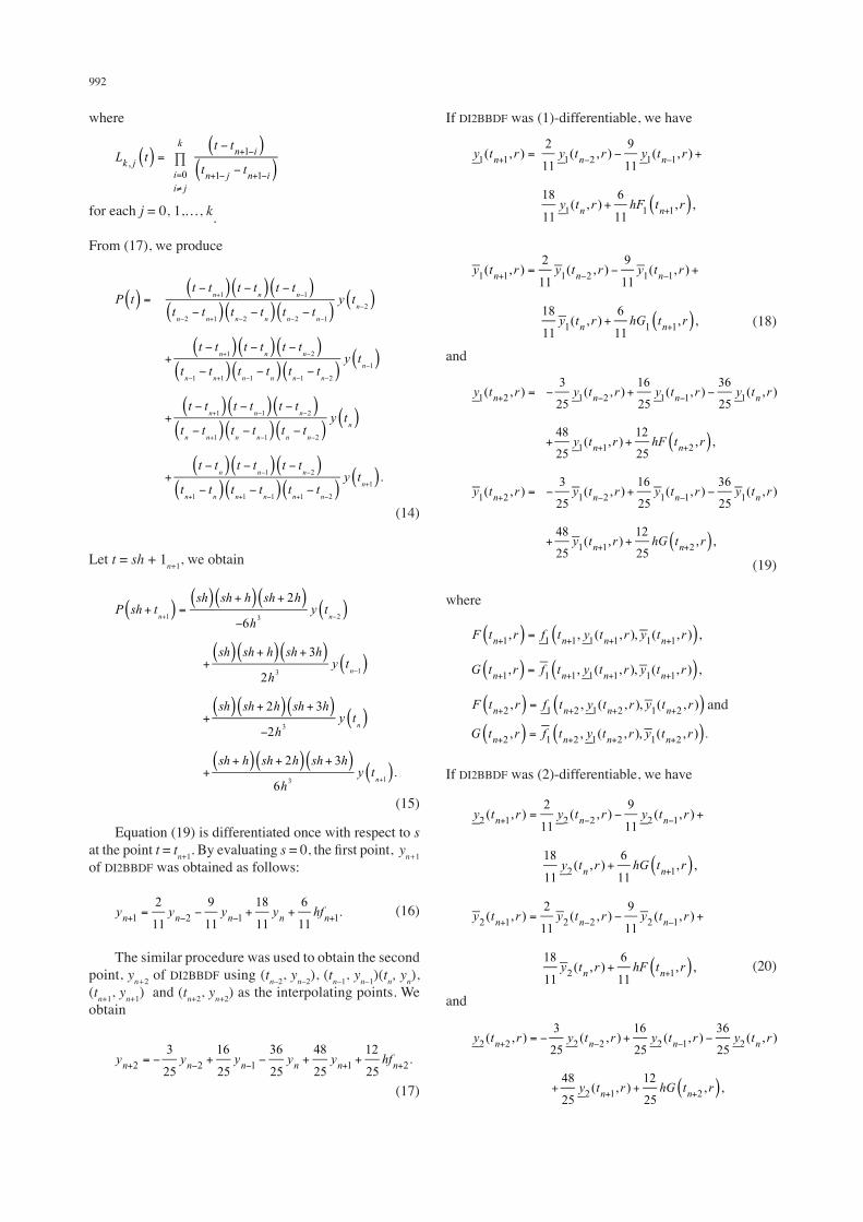
From (17), we produce
(14)
Let t = sh + 1n+1, we obtain
(15)
Equation (19) is differentiated once with respect to s at the point t = tn+1. By evaluating s = 0, the first point, yn+1 of DI2BBDF was obtained as follows:
(16)
The similar procedure was used to obtain the second point, yn+2 of DI2BBDF using (tn–2, yn–2), (tn–1, yn–1)(tn, yn), (tn+1, yn+1) and (tn+2, yn+2) as the interpolating points. We obtain
(17)
If DI2BBDF was (1)-differentiable, we have
(18)
and
(19)
where
and
If DI2BBDF was (2)-differentiable, we have
(20)
and

993
(21)
where
and
NUMERICAL EXPERIMENTS
In this section, two fuzzy initial value problems (FIVPs) were provided to test the effectiveness of FI2BBDF and DI2BBDF. All computations were carried out using C programming with step size 0.01 and the exact solutions of each test problems were determined using Maple software.Problem 1: Consider the FIVP (Balooch Shahryari & Salahshour 2012)
(22)
Let λ = 1 and I = [0,0.1]. Based on (4), (22) can be translated into a system of ODEs as follows:
where the (1)-differentiable solution at t = 0.1 is given by
Using the form of (5), we have the following system of ODEs:
where
was (2)-differentiable solution
Problem 2: Consider bank account problem (Mondal & Roy 2013)
(23)
The balance, y(t) of a bank account grows under continuous process given by yʹ(t) where c was the annual interest rate (c = 4%) and y(0, r) was the initial balance. Hence, (23) can be translated into a system of ODEs as follows:
where the (1)-differentiable solution at t = 0.1 was given by
Using the form of (5), we have the following system of ODEs:
where
was (2)-differentiable solution.
The numerical solutions of Problems 1 and 2 were shown in Tables 1 - 4 and Tables 5 – 8, respectively. In addition, the comparison of exact solutions and approximated solutions between FI2BBDF and DI2BBDF was illustrated in Figures 1 - 4. The notation and abbreviation used in the tables and figures take the following meaning:
r : Fuzzy numbers with bounded r-cut intervals
: Lower bounded approximated solution for Case 1
: Upper bounded approximated solution for Case 1
: Lower bounded exact solution for Case 1
: Upper bounded exact solution for Case 1
: Lower bounded approximated solution for Case 2
: Upper bounded approximated solution for Case 2
: Lower bounded exact solution for Case 2
: Upper bounded exact solution for Case 2
Error : or

994
TABLE 2. Numerical results of FI2BBDF for Problem 1 (Case 2)
r Error Error
0.0 -9.133647E-1 -9.139312E-1 5.664630E-4 9.133647E-1 9.139312E-1 5.664630E-40.1 -8.220283E-1 -8.225381E-1 5.098167E-4 8.220283E-1 8.225381E-1 5.098167E-40.2 -7.306918E-1 -7.311449E-1 4.531704E-4 7.306918E-1 7.311449E-1 4.531704E-40.3 -6.393553E-1 -6.397518E-1 3.965241E-4 6.393553E-1 6.397518E-1 3.965241E-40.4 -5.480188E-1 -5.483587E-1 3.398778E-4 5.480188E-1 5.483587E-1 3.398778E-40.5 -4.566824E-1 -4.569656E-1 2.832315E-4 4.566824E-1 4.569656E-1 2.832315E-40.6 -3.656366E-1 -3.655725E-1 2.265852E-4 3.653459E-1 3.655725E-1 2.265852E-40.7 -2.740094E-1 -2.741794E-1 1.699389E-4 2.740094E-1 2.741794E-1 1.699389E-40.8 -1.826729E-1 -1.827862E-1 1.132926E-4 1.826729E-1 1.827862E-1 1.132926E-40.9 -9.133647E-2 -9.139312E-2 5.664630E-5 9.133647E-2 9.139312E-2 5.664630E-51.0 0 0 0 0 0 0
TABLE 1. Numerical results of FI2BBDF for Problem 1 (Case 1)
r Y1 Error Error
0.0 -1.093521 -1.094174 6.536184E-4 1.093521 1.094174 6.536184E-40.1 -9.841686E-1 -9.847569E-1 5.882565E-4 9.841686E-1 9.847569E-1 5.882565E-40.2 -8.748165E-1 -8.753394E-1 5.228947E-4 8.748165E-1 8.753394E-1 5.228947E-40.3 -7.654645E-1 -7.659220E-1 4.575329E-4 7.654645E-1 7.659220E-1 4.575329E-40.4 -6.561124E-1 -6.565046E-1 3.921710E-4 6.561124E-1 6.565046E-1 3.921710E-40.5 -5.467603E-1 -5.470871E-1 3.268092E-4 5.467603E-1 5.470871E-1 3.268092E-40.6 -4.374083E-1 -4.376697E-1 2.614473E-4 4.374083E-1 4.376697E-1 2.614473E-40.7 -3.280562E-1 -3.282523E-1 1.960855E-4 3.280562E-1 3.282523E-1 1.960855E-40.8 -2.187041E-1 -2.188349E-1 1.307237E-4 2.187041E-1 2.188349E-1 1.307237E-40.9 -1.093521E-1 -1.094174E-1 6.536184E-5 1.093521E-1 1.094174E-1 6.536184E-51.0 0 0 0 0 0 0
TABLE 3. Numerical results of DI2BBDF for Problem 1 (Case 1)
r Y1 Error Error
0.0 -1.094353 -1.094174 1.784107E-4 1.094353 1.094174 1.784107E-40.1 -9.849174E-1 -9.847569E-1 1.605696E-4 9.849174E-1 9.847569E-1 1.605696E-40.2 -8.754822E-1 -8.753394E-1 1.427285E-4 8.754822E-1 8.753394E-1 1.427285E-40.3 -7.660469E-1 -7.659220E-1 1.248875E-4 7.660469E-1 7.659220E-1 1.248875E-40.4 -6.566116E-1 -6.565046E-1 1.070464E-4 6.566116E-1 6.565046E-1 1.070464E-40.5 -5.471763E-1 -5.470871E-1 8.920534E-5 5.471763E-1 5.470871E-1 8.920534E-50.6 -4.377411E-1 -4.376697E-1 7.136427E-5 4.377411E-1 4.376697E-1 7.136427E-50.7 -3.283058E-1 -3.282523E-1 5.352320E-5 3.283058E-1 3.282523E-1 5.352320E-50.8 -2.188705E-1 -2.188349E-1 3.568213E-5 2.188705E-1 2.188349E-1 3.568213E-50.9 -1.094353E-1 -1.094174E-1 1.784107E-5 1.094353E-1 1.094174E-1 1.784107E-51.0 0 0 0 0 0 0

995
TABLE 4. Numerical results of DI2BBDF for Problem 1 (Case 2)
r Error Error
0.0 -9.140915E-1 -9.139312E-1 1.603542E-4 9.140915E-1 9.139312E-1 1.603542E-40.1 -8.226824E-1 -8.225381E-1 1.443188E-4 8.226824E-1 8.225381E-1 1.443188E-40.2 -7.312732E-1 -7.311449E-1 1.282834E-4 7.312732E-1 7.311449E-1 1.282834E-40.3 -6.398641E-1 -6.397518E-1 1.122480E-4 6.398641E-1 6.397518E-1 1.122480E-40.4 -5.484549E-1 -5.483587E-1 9.621254E-5 5.484549E-1 5.483587E-1 9.621254E-50.5 -4.570458E-1 -4.569656E-1 8.017712E-5 4.570458E-1 4.569656E-1 8.017712E-50.6 -3.656366E-1 -3.655725E-1 6.414169E-5 3.656366E-1 3.655725E-1 6.414169E-50.7 -2.742275E-1 -2.741794E-1 4.810627E-5 2.742275E-1 2.741794E-1 4.810627E-50.8 -1.828183E-1 -1.827862E-1 3.207085E-5 1.828183E-1 1.827862E-1 3.207085E-50.9 -9.140915E-2 -9.139312E-2 1.603542E-5 9.140915E-2 9.139312E-2 1.603542E-51.0 0 0 0 0 0 0
TABLE 5. Numerical results of FI2BBDF for Problem 2 (Case 1)
r Y1 Error Error
0.0 9.539652E2 9.539662E2 9.278306E-4 1.103426E3 1.103427E3 1.073428E-30.1 9.601703E2 9.601712E2 9.338798E-4 1.090948E3 1.090950E3 1.061278E-30.2 9.663753E2 9.663762E2 9.399289E-4 1.078471E3 1.078472E3 1.049127E-30.3 9.725803E2 9.725813E2 9.459781E-4 1.065993E3 1.065994E3 1.036977E-30.4 9.787854E2 9.787863E2 9.520272E-4 1.053516E3 1.053517E3 1.024826E-30.5 9.849904E2 9.849914E2 9.580764E-4 1.041038E3 1.041039E3 1.012675E-30.6 9.911954E2 9.911964E2 9.641255E-4 1.028561E3 1.028562E3 1.000525E-30.7 9.974005E2 9.974014E2 9.701747E-4 1.016083E3 1.016084E3 9.883744E-40.8 1.003606E3 1.003606E3 9.762238E-4 1.003606E3 1.003606E3 9.762238E-40.9 1.009811E3 1.009812E3 9.822730E-4 9.911279E2 9.911289E2 9.640733E-41.0 1.016016E3 1.016017E3 9.883221E-4 9.786504E2 9.786513E2 9.519227E-4
TABLE 6. Numerical results of FI2BBDF for Problem 2 (Case 2)
r Error Error
0.0 9.534252E2 9.534262E2 9.274126E-4 1.103966E3 1.103967E3 1.073846E-30.1 9.596978E2 9.596987E2 9.335140E-4 1.091421E3 1.091422E3 1.061643E-30.2 9.659703E2 9.659712E2 9.396154E-4 1.078876E3 1.078877E3 1.049441E-30.3 9.722428E2 9.722438E2 9.457168E-4 1.066331E3 1.066332E3 1.037238E-30.4 9.785154E2 9.785163E2 9.518182E-4 1.053786E3 1.053787E3 1.025035E-30.5 9.847879E2 9.847889E2 9.579196E-4 1.041241E3 1.041242E3 1.012832E-30.6 9.910604E2 9.910614E2 9.640210E-4 1.028696E3 1.028697E3 1.000629E-30.7 9.973330E2 9.973339E2 9.701224E-4 1.016151E3 1.016152E3 9.884266E-40.8 1.003606E3 1.003606E3 9.762238E-4 1.003606E3 1.003606E3 9.762238E-40.9 1.009878E3 1.009879E3 9.823252E-4 9.910604E2 9.910614E2 9.640210E-41.0 1.016151E3 1.016152E3 9.884266E-4 9.785154E2 9.785163E2 9.518182E-4
996
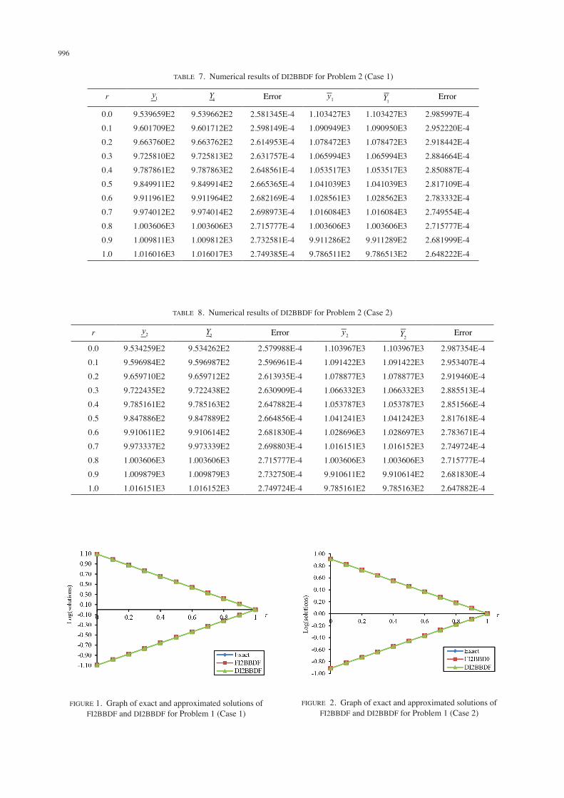
TABLE 8. Numerical results of DI2BBDF for Problem 2 (Case 2)
r Error Error
0.0 9.534259E2 9.534262E2 2.579988E-4 1.103967E3 1.103967E3 2.987354E-40.1 9.596984E2 9.596987E2 2.596961E-4 1.091422E3 1.091422E3 2.953407E-40.2 9.659710E2 9.659712E2 2.613935E-4 1.078877E3 1.078877E3 2.919460E-40.3 9.722435E2 9.722438E2 2.630909E-4 1.066332E3 1.066332E3 2.885513E-40.4 9.785161E2 9.785163E2 2.647882E-4 1.053787E3 1.053787E3 2.851566E-40.5 9.847886E2 9.847889E2 2.664856E-4 1.041241E3 1.041242E3 2.817618E-40.6 9.910611E2 9.910614E2 2.681830E-4 1.028696E3 1.028697E3 2.783671E-40.7 9.973337E2 9.973339E2 2.698803E-4 1.016151E3 1.016152E3 2.749724E-40.8 1.003606E3 1.003606E3 2.715777E-4 1.003606E3 1.003606E3 2.715777E-40.9 1.009879E3 1.009879E3 2.732750E-4 9.910611E2 9.910614E2 2.681830E-41.0 1.016151E3 1.016152E3 2.749724E-4 9.785161E2 9.785163E2 2.647882E-4
TABLE 7. Numerical results of DI2BBDF for Problem 2 (Case 1)
r Y1 Error Error
0.0 9.539659E2 9.539662E2 2.581345E-4 1.103427E3 1.103427E3 2.985997E-40.1 9.601709E2 9.601712E2 2.598149E-4 1.090949E3 1.090950E3 2.952220E-40.2 9.663760E2 9.663762E2 2.614953E-4 1.078472E3 1.078472E3 2.918442E-40.3 9.725810E2 9.725813E2 2.631757E-4 1.065994E3 1.065994E3 2.884664E-40.4 9.787861E2 9.787863E2 2.648561E-4 1.053517E3 1.053517E3 2.850887E-40.5 9.849911E2 9.849914E2 2.665365E-4 1.041039E3 1.041039E3 2.817109E-40.6 9.911961E2 9.911964E2 2.682169E-4 1.028561E3 1.028562E3 2.783332E-40.7 9.974012E2 9.974014E2 2.698973E-4 1.016084E3 1.016084E3 2.749554E-40.8 1.003606E3 1.003606E3 2.715777E-4 1.003606E3 1.003606E3 2.715777E-40.9 1.009811E3 1.009812E3 2.732581E-4 9.911286E2 9.911289E2 2.681999E-41.0 1.016016E3 1.016017E3 2.749385E-4 9.786511E2 9.786513E2 2.648222E-4
FIGURE 1. Graph of exact and approximated solutions of FI2BBDF and DI2BBDF for Problem 1 (Case 1)
FIGURE 2. Graph of exact and approximated solutions of FI2BBDF and DI2BBDF for Problem 1 (Case 2)

997
that both methods were suitable for solving FDEs. Future work is in progress on extending the DI2BBDF method for solving higher order FDEs.
REFERENCES
Abbasbandi, S. & Viranloo, T.A. 2002. Numerical solutions of fuzzy differential equations by Taylor method. Comp. Method in Applied Mathematics 2: 113-124.
Ahmad, M.Z. & Hasan, M K. 2011. A new fuzzy version of Euler’s method for solving differential equations with fuzzy initial values. Sains Malaysiana 40(6): 651-657.
Balooch Shahryari, M.R. & Salahshour, S. 2012. Improved predictor corrector method for solving fuzzy differential equations under generalized differentiability. Journal of Fuzzy Set Valued Analysis 2012: 1-16.
Bede, B., Bhaskar, T.G. & Lakshmikantham, V. 2007. Perspective of fuzzy initial value problems. Communications in Applied Analysis 11: 339-358.
Bede, B. & Gal, S.G. 2005. Generalizations of the differentiability of fuzzy-number-valued functions with applications to fuzzy differential equations. Fuzzy Sets and Systems 151: 581-599.
Chalco-Cano, Y. & Roman-Flores, H. 2008. On new solutions of fuzzy differential equations. Chaos, Solitons and Fractals 38: 112-119.
Ghazanfari, B. & Shakerami, A. 2012. Numerical solutions of fuzzy differential equations by extended Runge-Kutta-like formulae of order four. Fuzzy Sets and Systems 189(1): 74-91.
Ibrahim, Z.B., Suleiman, M.B. & Nasir, N.A.A.M. 2011. Convergence of the 2-point block backward differentiation formulas. Applied Mathematical Sciences 5(70): 3473-3480.
Ibrahim, Z.B., Suleiman, M.B. & Othman, K.I. 2008. Fixed coefficients block backward differentiation formulas for the numerical solution of stiff ordinary differential equations. European Journal of Scientific Research 21(3): 508-520.
Ibrahim, Z.B., Suleiman, M.B. & Othman, K.I. 2007. Implicit r-point block backward differentiation formula for solving first order stiff odes. Applied Mathematics and Computation 186: 558-565.
Ibrahim, Z.B., Johari, R. & Ismail, F. 2003. On the stability of block backward differentiation formulae. Matematika 19(2): 83-89.
Mondal, S.P. & Roy, T.K. 2013. First order linear homogeneous ordinary differential equation in fuzzy environment based on laplace transform. Journal of Fuzzy Set Valued Analysis 2013: 1-18.
DISCUSSION
From all tabulated results, it was apparent that the approximated solutions of both methods tend to the exact solutions. The approximated solutions showed that was an increasing function and was a decreasing function for r ∈ [0,1]. This was expected due to Definition 2.2. However, it should be noted that in Problem 1, the solution obtained for r = 1.0 was whereas in Problem 2, the solution obtained for r = 1.0 was
. This satisfies the Definition 3.1 where Problem 1 possesses strong solutions for r = [0,1] while Problem 2 possesses strong solutions for r = [0,0.8] and weak solutions for r ∈ [0.9,1]. Next, we were interested to discuss and compare the numerical results obtained by FI2BBDF and DI2BBDF in term of accuracy. Note that Tables 1 - 2 and Tables 5 - 6 show the exact and approximated solutions of FI2BBDF for solving Problems 1 and 2, respectively. Tables 3 - 4 and Tables 7 - 8 show the exact and approximated solutions of DI2BBDF for solving Problems 1 and 2, respectively. From Tables 1 - 8, it was obvious that the DI2BBDF was more accurate than FI2BBDF for both tested problems. This may due to the derivation of diagonally implicit method which involves less interpolating point. Furthermore, the accuracy of DI2BBDF for Case 2 (Table 4) was better than Case 1 (Table 3) when r ∈ [0.4,1]. However, the pattern of accuracy for Case 1 (Table 7) was almost similar to that in Case 2 (Table 8). This indicates the importance of generalized differentiability concept for numerical solution of fuzzy problems.
CONCLUSION
In this paper we present the numerical solution of FDEs using FI2BBDF and DI2BBDF under generalized differentiability concept. We have shown that the solution of FDEs was not unique since it has two types of differentiability to be considered. Therefore we can choose the solution which better reflects the behavior of any real system. From the numerical results, the DI2BBDF performs better than FI2BBDF in term of accuracy. Overall it can be concluded
FIGURE 3. Graph of exact and approximated solutions of FI2BBDF and DI2BBDF for Problem 2 (Case 1)
r
FIGURE 4. Graph of exact and approximated solutions of FI2BBDF and DI2BBDF for Problem 2 (Case 2)
r

998
Puri, M.L. & Ralescu, D. 1983. Differential for fuzzy function. J. Math. Anal. Appl. 91: 552-558.
Shokri, J. 2007. Numerical solution of fuzzy differential equations. Applied Mathematical Sciences 1: 2231-2246.
Zawawi, I.S.M., Ibrahim, Z.B., Ismail, F. & Majid, Z.A. 2012. Diagonally implicit block backward differentiation formulas for solving ordinary differential equations. International Journal of Mathematics and Mathematical Sciences Article ID 767328.
Iskandar Shah Mohd ZawawiDepartment of MathematicsFaculty of ScienceUniversiti Putra Malaysia43400 Serdang, Selangor Darul EhsanMalaysia
Zarina Bibi Ibrahim*Institute for Mathematical ResearchUniversiti Putra Malaysia43400 Serdang, Selangor Darul EhsanMalaysia
Corresponding author: [email protected]
Received: 7 April 2015Accepted: 5 January 2015