Block-proximal methods with spatiallyadapted acceleration

Tuomo Valkonen˚

September 30, 2016

We propose a class of primal–dual block-coordinate descent methodsbased on blockwise proximal steps. The methods can be executed eitherstochastically, randomly executing updates of each block of variables, orthe methods can be executed deterministically, featuring performance-improving blockwise adapted step lengths. Our work improves upon severalprevious stochastic primal–dual methods in that we do not require a full dualupdate in an accelerated method; both the primal and dual can be updatedstochastically in blocks. We moreover provide convergence rates withoutthe strong assumption of all functions being strongly convex or smooth:a mixed Op1N 2q ` Op1N q for an ergodic gap and individual stronglyconvex primal blocks. Within the context of deterministic methods, ourblockwise adapted methods provide improvements on our earlier work onsubspace accelerated methods. We test the proposed methods on variousimage processing problems.

1. Introduction

We want to eciently solve optimisation problems of the form

minx

Gpxq ` F pKxq, (1.1)

arising from the variational regularisation of image processing and inverse problems.We assume G : X Ñ R and F : Y Ñ R to be convex, proper, and lower semicontinuousfunctionals on Hilbert spaces X and Y , respectively, and K P LpX ;Y q to be a boundedlinear operator.

Several rst-order optimisation methods have been developed for (1.1), typically withboth G and F convex, and K linear, but recently also accepting a level of non-convexityand non-linearity [1–4]. Since at least one of G or F is typically non-smooth—popularregularisers for image processing are non-smooth, such as [5–7]—eective primal algo-rithms operating directly on the form (1.1), are typically a form of classical forward–backward splitting, occasionally going by the name of iterative soft-thresholding [8–10].

If G is separable, Gpx1, . . . ,xmq “řm

j“1G jpx jq, problem (1.1) becomes

minx

mÿ

j“1G jpx jq ` F pKxq. (1.2)

˚Department of Mathematical Sciences, University of Liverpool, United Kingdom.tuomo.valkonen@iki.fi

1

In big data optimisation, various forward–backward block-coordinate descent methodshave been developed for this type of problems, or an alternative dual formulation.At each step of the optimisation method, they only update a subset of the blocks x j ,randomly in parallel, see e.g. the review [11] and the original articles [12–22]. TypicallyF is assumed smooth. Often, in these methods, each of the functions G j is assumedstrongly convex. Besides parallelism, one advantage of these methods is them beingable to exploit the local blockwise factor of smoothness (Lipschitz gradient) of F andK . This can be better than the global factor, and helps to obtain improved convergencecompared to standard methods.

Unfortunately, primal-only and dual-only stochastic approaches are rarely applicableto imaging problems that do not satisfy the separability and smoothness requirementssimultaneously, at least not without additional Moreau–Yosida (aka. Huber, aka. Nes-terov) regularisation. Generally, even without the splitting of the problem of the intoblocks, primal-only or dual-only approaches, as discussed above, can be inecienton more complicated problems, as the steps of the algorithms become very expensiveoptimisation problems themselves. This diculty can often be circumvented throughprimal-dual approaches. If F is convex, and F˚ denotes the conjugate of F , the problem(1.1) can be written in the min-max form

minx

maxy

Gpxq ` xKx ,yy ´ F˚pxq, (1.3)

If G is also convex, a popular algorithm for (1.3) is the Chambolle–Pock method [23, 24],also classied as the Primal-Dual Hybrid Gradient Method (Modied) or PDHGM in [25].The method consists of alternating proximal steps on x and y , combined with an over-relaxation step that ensures convergence. The PDHGM is closely-related to the classicalAlternating Direction Method of Multipliers (ADMM, [26]). Both the PDHGM andADMM bear close relationship to Douglas–Rachford splitting [27, 28] and the splitBregman method [29, 30]. These relationships are discussed in detail in [25, 31].

While early work on block-coordinate descent methods concentrated on primal-onlyor dual-only algorithms, recently primal-dual algorithms based on the ADMM andthe PDHGM have been proposed [32–38]. Besides [32, 33, 38] that have restrictivesmoothness and strong convexity requirements, little is known about the convergencerates of these algorithms. Interestingly, a direct blockwise version of ADMM for (1.2) ishowever infeasible [39].

The convergence of the PDHGM can be accelerated from the basic rate Op1N q toOp1N 2q if G (equivalently F˚) is strongly convex [23]. However, saddle-point formula-tions (1.3) of important problems often lack strong convexity on the entire domain of G .These include any problem with higher-order TGV [6] or ICTV [7] regularisation, aswell as such simple problems as deblurring with any regularisation term. Motivatedby this, we recently showed in [3] that acceleration schemes can still produce con-vergence with a mixed rate, Op1N 2q with respect to initialisation, and Op1N q withrespect to “residual variables”, if G is only partially strongly convex. This means withx “ px1, . . . ,xmq for some block k and a factor γk ą 0 the condition

Gpx 1q ´Gpxq ě xz,x 1 ´ xy `γk2x 1k ´ xk

2, (1.4)

over all x 1 and subgradients z P BGpxq. This property can be compared to partialsmoothness on manifolds [40, 41], used to study the fast convergence of standardmethods to submanifolds [42].

Under the condition (1.4), the iterates tx iku8i“0 of the “partially accelerated” methods

proposed in [3] will convergence fast to an optimal solution pxk , while nothing is knownabout the convergence of non-strongly-convex blocks. In Section 2 of this work, we

2

improve this analysis to be able to deal with partial steps, technically non-invertiblestep-length operators. We also allow the steps to be chosen stochastically. Some ofthe abstract proofs that are relatively minor generalisations of those in [3], we haveleft to Appendix A. From this abstract analysis, we derive in Sections 3 and 4 bothstochastic and deterministic block-proximal primal-dual methods with the novelty ofhaving local or blockwise step lengths. These can either be adapted dynamically to theactual sequence of block updates taken by the method, or taken deterministically withthe goal of reducing communication in parallel implementations. As the most extremecase, which we consider in several of our image processing experiments in the nalSection 5, our methods can have pixelwise-adapted step lengths.

The stochastic variants of our methods do not require the entire dual variable to beupdated, it can also be randomised under light compatibility conditions on the primal anddual blocks. In the words of [38], our methods are “doubly-stochastic”. Our additionaladvances here are the convergence analysis—proving mixed Op1N 2q `Op1N q ratesof both the (squared) iterates and an ergodic gap—not being restricted to single-blockupdates, and not demanding strong convexity or smoothness from the entire problem,only individual blocks of interest.

2. A general method with non-invertible step operators

2.1. Background

To make the notation denite, we writeLpX ;Y q for the space of bounded linear operatorsbetween Hilbert spaces X and Y . The identity operator we denote by I . For T ,S PLpX ;X q, we use T ě S to mean that T ´ S is positive semidenite; in particular T ě 0means thatT is positive semidenite. Also for possibly non-self-adjointT , we introducethe inner product and norm-like notations

xx ,zyT :“ xTx ,zy, and xT :“b

xx ,xyT , (2.1)

the latter only dened for positive semi-denite T . We write T » T 1 if xx ,xyT 1´T “ 0for all x .

Denoting R :“ r´8,8s, we now let G : X Ñ R and F˚ : Y Ñ R be given convex,proper, lower semicontinuous functionalsG : X Ñ R and F˚ : Y Ñ R on Hilbert spacesX and Y . We also let K P LpX ;Y q be a bounded linear operator. We then wish to solvethe minimax problem

minxPX

maxyPY

Gpxq ` xKx ,yy ´ F˚pyq, (P)

assuming the existence of a solution pu “ ppx ,pyq satisfying the optimality conditions

´ K˚py P BGppxq, and Kpx P BF˚ppyq. (OC)

The primal-dual method of Chambolle and Pock [23] for (P) consists of iterating thesystem

x i`1 :“ pI ` τiBGq´1px i ´ τiK

˚y iq, (2.2a)x i`1 :“ ωipx

i`1 ´ x iq ` x i`1, (2.2b)y i`1 :“ pI ` σi`1BF

˚q´1py i ` σi`1Kxi`1q. (2.2c)

In the basic version of the algorithm, ωi “ 1, τi ” τ0, and σi ” σ0, assuming thatthe step length parameters satisfy τ0σ0K

2 ă 1. The method has Op1N q rate for theergodic duality gap. If G is strongly convex with factor γ , we may accelerate

ωi :“ 1a

1` 2γτi , τi`1 :“ τiωi , and σi`1 :“ σiωi , (2.3)

3

to achieveOp1N 2q convergence rates. To motivate our later choices, we observe that σ0is never needed if we equivalently parametrise the algorithm by δ “ 1´ K2τ0σ0 ą 0.

In [3], we extended the algorithm (2.2) & (2.3) to partially strongly convex problems.For suitable step length operators Ti P LpX ;X q and Σi P LpY ;Y q, as well as an over-relaxation parameter rωi ą 0, it consists of the iterations

x i`1 :“ pI `TiBGq´1px i ´TiK

˚y iq, (2.4a)x i`1 :“ rωipx

i`1 ´ x iq ` x i`1, (2.4b)y i`1 :“ pI ` Σi`1BF

˚q´1py i ` Σi`1Kxi`1q, (2.4c)

The diagonally preconditioned algorithm of [43] also ts into this form. For specicchoices of Ti , Σi , and rωi , and under additional conditions on G and F˚, we were able toobtain mixed Op1N 2q `Op1N q convergence rates of an ergodic duality gap, as wellas the squared distance of the primal iterates within a subspace on which G is stronglyconvex.

Let us momentarily assume that the operators Ti and Σi`1 are invertible. Following[3, 44], we may with the general variable splitting notation

u “ px ,yq,

write the system (2.4) as

0 P Hpui`1q `Mipui`1 ´ uiq, (PP0)

for the monotone operator

Hpuq :“ˆ

BGpxq ` K˚yBF˚pyq ´ Kx

˙

, (2.5)

and the preconditioning or step-length operator

Mi :“ˆ

T´1i ´K˚

´rωiK Σ´1i`1

˙

. (2.6)

With these operators, the optimality conditions (OC) can also be encoded as 0 P Hppuq.

Remark 2.1 (A word about the indexing). The reader may have noticed that the stepsof (2.2) and (2.4) involve Ti and Σi`1, with distinct indices. This is mainly to maintainin (2.3) the identity τiσi “ τi`1σi`1 from [23]. On the other hand the proximal pointformulation necessitates x-rst ordering of the steps (2.2) in contrast to the y-rst orderin [23]. Thus our y i`1 is their y i .

2.2. Non-invertible step length operators

What if Ti and Σi`1 are non-invertible? The algorithm (2.4) of course works, but howabout the proximal point version (PP0)? We want to use the form (PP0), because itgreatly eases the analysis of the method.

Dening

Wi`1 :“ˆ

Ti 00 Σi`1

˙

, and (for now) Li`1 “

ˆ

I ´TiK˚

´rωiΣi`1K I

˙

, (2.7)

the method (2.4) can also be written

Wi`1Hpui`1q ` Li`1pu

i`1 ´ uiq Q 0. (PP)

4

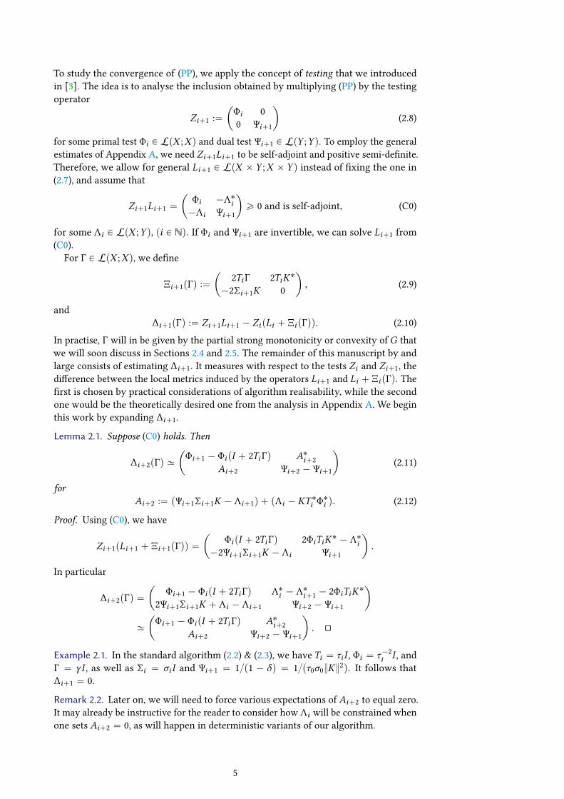
To study the convergence of (PP), we apply the concept of testing that we introducedin [3]. The idea is to analyse the inclusion obtained by multiplying (PP) by the testingoperator

Zi`1 :“ˆ

Φi 00 Ψi`1

˙

(2.8)

for some primal test Φi P LpX ;X q and dual test Ψi`1 P LpY ;Y q. To employ the generalestimates of Appendix A, we need Zi`1Li`1 to be self-adjoint and positive semi-denite.Therefore, we allow for general Li`1 P LpX ˆ Y ;X ˆ Y q instead of xing the one in(2.7), and assume that

Zi`1Li`1 “

ˆ

Φi ´Λ˚i´Λi Ψi`1

˙

ě 0 and is self-adjoint, (C0)

for some Λi P LpX ;Y q, pi P Nq. If Φi and Ψi`1 are invertible, we can solve Li`1 from(C0).

For Γ P LpX ;X q, we dene

Ξi`1pΓq :“ˆ

2TiΓ 2TiK˚´2Σi`1K 0

˙

, (2.9)

and∆i`1pΓq :“ Zi`1Li`1 ´ ZipLi ` ΞipΓqq. (2.10)

In practise, Γ will in be given by the partial strong monotonicity or convexity of G thatwe will soon discuss in Sections 2.4 and 2.5. The remainder of this manuscript by andlarge consists of estimating ∆i`1. It measures with respect to the tests Zi and Zi`1, thedierence between the local metrics induced by the operators Li`1 and Li ` ΞipΓq. Therst is chosen by practical considerations of algorithm realisability, while the secondone would be the theoretically desired one from the analysis in Appendix A. We beginthis work by expanding ∆i`1.

Lemma 2.1. Suppose (C0) holds. Then

∆i`2pΓq »

ˆ

Φi`1 ´ ΦipI ` 2TiΓq A˚i`2Ai`2 Ψi`2 ´ Ψi`1

˙

(2.11)

forAi`2 :“ pΨi`1Σi`1K ´ Λi`1q ` pΛi ´ KT ˚i Φ

˚i q. (2.12)

Proof. Using (C0), we have

Zi`1pLi`1 ` Ξi`1pΓqq “

ˆ

ΦipI ` 2TiΓq 2ΦiTiK˚ ´ Λ˚i

´2Ψi`1Σi`1K ´ Λi Ψi`1

˙

.

In particular

∆i`2pΓq “

ˆ

Φi`1 ´ ΦipI ` 2TiΓq Λ˚i ´ Λ˚i`1 ´ 2ΦiTiK˚

2Ψi`1Σi`1K ` Λi ´ Λi`1 Ψi`2 ´ Ψi`1

˙

»

ˆ

Φi`1 ´ ΦipI ` 2TiΓq A˚i`2Ai`2 Ψi`2 ´ Ψi`1

˙

.

Example 2.1. In the standard algorithm (2.2) & (2.3), we have Ti “ τi I , Φi “ τ´2i I , and

Γ “ γ I , as well as Σi “ σi I and Ψi`1 “ 1p1 ´ δq “ 1pτ0σ0K2q. It follows that

∆i`1 “ 0.

Remark 2.2. Later on, we will need to force various expectations of Ai`2 to equal zero.It may already be instructive for the reader to consider how Λi will be constrained whenone sets Ai`2 “ 0, as will happen in deterministic variants of our algorithm.

5

2.3. Stochastic variants

Just before commencing with the i:th iteration of (PP), let us choose Ti and Σi`1 ran-domly, only based on the information we have gathered beforehand. We denote thisinformation by Oi´1, including the specic random realisations of Ti´1 and Σi . Techni-cally Oi´1 is a σ -algebra, and satises Oi´1 Ă Oi . For details on the measure-theoreticapproach to probability, we refer the reader to [45], here we merely recall some basicconcepts.

Definition 2.1. We denote by pΩ,O,Pq the probability space consisting of the set Ωof possible realisation of a random experiment, by O a σ -algebra on Ω, and by P aprobability measure on pΩ,Oq. We denote the expectation corresponding to P by E,the conditional probability with respect to a sub-σ -algebra O1 Ă O by Pr ¨ |O1s, and theconditional expectation by Er ¨ |O1s.

We also use the next non-standard notation.

Definition 2.2. If O is a σ -algebra on the space Ω, we denote by RpO;V q the space ofV -valued random variables A, such that A : Ω Ñ V is O-measurable.

We frequently abuse notation, and use A as if it were a variable in V . For example,Ti P RpOi ;LpX ;X qq, but we generally think of Ti directly as an operator in LpX ;X q.Indeed, in our work, random variables and probability spaces only become apparentin the expectations E, and probabilities P, otherwise everything is happening in theunderlying space V . The spaces RpO;V q mainly serve to clarify the measurabilitywith respect to dierent σ -algebras Oi , that is, the algorithm iteration on which therealisation of a random variable is known.Oi thus includes all our knowledge prior to iteration i , with the interpretation that

the random realisations of Ti and Σi`1 are also known just before iteration i begins.Formally

Ti P RpOi ;LpX ;X qq, and Σi`1 P RpOi ;LpY ;Y qq.

Assuming that also Φi P RpOi ;LpX ;X qq and Ψi`1 P RpOi ;LpY ;Y qq, we deduce from(PP) that x i`1 P RpOi ;X q and y i`1 P RpOi ;Y q. We say that any variable, e.g., x i`1 P

RpOi ;X q, that can be computed from the information in Oi to be deterministic withrespect to Oi . Then in particular Erx i`1|Ok s “ x i`1 for all k ě i .

2.4. Basic estimates on the abstract proximal point iteration

To derive convergence rate estimates, we start by formulating abstract forms of partialstrong monotonicity. As a rst step, we take subsets of operators

T Ă LpX ;X q, and S Ă LpY ;Y q.

We then suppose that BG is partially strongly T -monotone, which we take to mean

xBGpx 1q ´ BGpxq, rT ˚px 1 ´ xqy ě x 1 ´ x2rT Γ, px ,x 1 P X ; rT P T q (G-PM)

for some linear operator 0 ď Γ P LpX ;X q. The operator rT P T acts as a testing operator.Similarly, we assume that BF˚ is S-monotone in the sense

xBF˚py 1q ´ BF˚pyq,rΣ˚py 1 ´ yqy ě 0, py ,y 1 P Y ; rΣ P Sq. (F˚-PM)

Example 2.2. Gpxq “ 12f ´ Ax2 satises (G-PM) with Γ “ A˚A and T “ LpX ;X q.

Indeed, we calculate x∇Gpx 1q ´ ∇Gpxq, rT ˚px 1 ´ xqy “ xA˚Apx 1 ´ xq, rT ˚px 1 ´ xqy “x 1 ´ x2

rT Γ.

6

Example 2.3. If F˚pyq “řn

`“1 F˚`py`q for y “ py1, . . . ,ynqwith each F˚

`convex, then F˚

satises (F˚-PM) with S “ třn

`“1 β`Q` | β` ě 0u for Q`y :“ y` . Indeed, the condition(F˚-PM) simply splits into separate monotonicity conditions for each BF˚

`, (` “ 1, . . . ,n).

The fundamental estimate that forms the basis of all our convergence results, is thefollowing. We note that the theorem does not yet prove convergence, but to do so wehave to estimate the “penalty sum” involving the operators ∆i`2, as well as the operatorZN`1LN`1. This is the content of the much of the rest of this paper. Moreover, toderive more meaningful “on average” results in the stochastic setting, we will take theexpectation of (2.13).

Theorem 2.1. Let us be given K P LpX ;Y q, and convex, proper, lower semicontinu-ous functionals G : X Ñ R and F˚ : Y Ñ R on Hilbert spaces X and Y , satisfy-ing (G-PM) and (F˚-PM) for some 0 ď Γ P LpX ;X q. Suppose the (random) operatorsTi ,Φi P RpOi ;LpX ;X qq and Σi`1,Ψi`1 P RpOi ;LpY ;Y qq satisfy ΦiTi P RpOi ;T q andΨi`1Σi`1 P RpOi ;Sq for each i P N. If, moreover, (C0) holds, then the iteratesui “ px i ,y iqof the proximal point iteration (PP) satisfy for all N ě 1 the estimate

uN ´ pu2ZN`1LN`1`

N´1ÿ

i“0ui`1 ´ ui2Zi`1Li`1

ď u0 ´ pu2Z0L0`

N´1ÿ

i“0ui`1 ´ pu2∆i`2pΓq

.

(2.13)

As the proof is a relatively straightforward improvement of [3, Theorem 2.1] tonon-invertible Ti and Σi , we relegate it to Appendix A.

2.5. Estimates on an ergodic duality gap

We may also prove the convergence of an ergodic duality gap. For this, the abstractmonotonicity assumptions (G-PM) and (F˚-PM) are not enough, and we need analogousconvexity formulations. We nd it most straightforward to formulate these conditionsdirectly in the stochastic setting. Namely we assume for all N ě 1 that wheneverrTi P RpOi ;T q and x i`1 P RpOi ;X q for each i “ 0, . . . ,N ´ 1, and that

řN´1i“0 ErrTi s “ I ,

then for some 0 ď Γ P LpX ;X q holds

G

˜

N´1ÿ

i“0ErrT ˚i x

i`1s

¸

´Gppxq ěN´1ÿ

i“0E

„

xBGpx i`1q, rT ˚i pxi`1 ´ pxqy `

12x i`1 ´ px2

rTi Γ

.

(G-EC)Analogously, we assume whenever rΣi`1 P RpOi ;Sq and y i`1 P RpOi ;Y q for eachi “ 0, . . . ,N ´ 1 with

řN´1i“0 ErrΣi`1s “ I that

F˚

˜

N´1ÿ

i“0ErrΣ˚i`1y

i`1s

¸

´ F˚ppyq ěN´1ÿ

i“0E”

xBF˚py i`1q,rΣ˚i`1pyi`1 ´ pyqy

ı

. (F˚-EC)

If everything is deterministic, (G-EC) and (F˚-EC) with N “ 1 imply (G-PM) and(F˚-PM).

Example 2.4. If rΣi`1 “ rσi`1I for some (random) scalar rσi`1, then it is easy to verify(F˚-EC) using Jensen’s inequality. We will generalise this example in Section 3.2.

Further, we assume for some ηi ą 0 that

ErT ˚i Φ˚i s “ ηi I , and ErΨi`1Σi`1s “ ηi I , pi ě 1q, (CG)

and for

ζN :“N´1ÿ

i“0ηi (2.14)

7

dene the ergodic sequences

rxN :“ ζ´1N E

«

N´1ÿ

i“0T ˚i Φ

˚i x

i`1

ff

, and ryN :“ ζ´1N E

«

N´1ÿ

i“0Σ˚i`1Ψ

˚i`1y

i`1

ff

. (2.15)

These sequences will eventually be generated through the application of (G-EC) and(F˚-EC) with rTi :“ ΦiTi and rΣi :“ ΨiΣi . Finally, we introduce the duality gap

Gpx ,yq :“`

Gpxq ` xpy ,Kxy ´ F ppyq˘

´`

Gppxq ` xy ,Kpxy ´ F˚pyq˘

. (2.16)

Then we have:

Theorem 2.2. Let us be given K P LpX ;Y q, and convex, proper, lower semicontinuousfunctionals G : X Ñ R and F˚ : Y Ñ R on Hilbert spaces X and Y , satisfying (G-PM),(F˚-PM), (G-EC) and (F˚-EC) for some 0 ď Γ P LpX ;X q. Suppose the (random) operatorsTi ,Φi P RpOi ;LpX ;X qq and Σi`1,Ψi`1 P RpOi ;LpY ;Y qq satisfy ΦiTi P RpOi ;T q andΨi`1Σi`1 P RpOi ;Sq for each i P N. If, moreover, (C0) and (CG) hold, then the iteratesui “ px i ,y iq of the proximal point iteration (PP) satisfy for all N ě 1 the estimate

E

«

xN ´ px2ZN`1LN`1`

N´1ÿ

i“0ui`1 ´ ui2Zi`1Li`1

ff

` ζNGprxN ,ryN q

ď u0 ´ pu2Z0L0`

N´1ÿ

i“0Erui`1 ´ pu2∆i`2pΓ2qs. (2.17)

Again, the proof is in Appendix A.

Remark 2.3. The dierence between ∆i`2pΓ2q and ∆i`2pΓq in (2.17) and (2.13) corre-sponds to the fact [23, 46] that in (2.2) we need slower ωi “ 1

?1` γτi compared to

(2.3), to get Op1N 2q convergence of the gap. The scheme (2.3) is only known to yieldconvergence of the iterates.

2.6. Estimates on another ergodic duality gap

The condition (CG) does not hold for the basic non-stochastic accelerated method (2.2)& (2.3), which would satisfy τiϕi “ ψσi for a suitable constant ψ and ϕi “ τ´2

i ; seeExample 2.1. We therefore assume for some ηi P R that

ErT ˚i Φ˚i s “ ηi I , and ErΨiΣi s “ ηi I , pi ě 1q, (CG˚)

and for

ζ ,N :“N´1ÿ

i“1ηi (2.18)

dene

rx ,N :“ ζ´1,NE

«

N´1ÿ

i“1T ˚i Φ

˚i x

i`1

ff

, and ry ,N :“ ζ´1,NE

«

N´1ÿ

i“1Σ˚i Ψ

˚i y

i

ff

. (2.19)

These variables give our new duality gap. Our original ergodic variables will howeverturn out to be the only possibility for doubly-stochastic methods. The convergenceresult is:

Theorem 2.3. In Theorem 2.2, let us assume Eq. (CG˚) in place of Eq. (CG). Then (2.17)holds with ζ ,NGprx ,N ,ry ,N q in place of ζNGprxN ,ryN q.

8

Once again, the proof is in Appendix A.

Remark 2.4. Technically, in Theorems 2.1 to 2.3, we do not need Ti , Φi , Σi`1, andΨi`1 deterministic with respect to Oi . It is sucient that Ti ,Φi P RpO;LpX ;X qq andΣi`1,Ψi`1 P RpO;LpY ;Y qq satisfy ΦiTi P RpO;T q and Ψi`1Σi`1 P RpO;Sq for eachi P N. For consistency, we have however made the stronger assumptions, which we willstart needing from now on.

2.7. Simplifications and summary so far

We assume the existence of some xed δ ą 0, and bounds bi`2prΓq dependent on ourchoice of rΓ P LpX ;X q such that

ErZi`2Li`2|Oi s ě

ˆ

δΦi`1 00 0

˙

, and (C1)

Erui`1 ´ pu2∆i`2prΓq

s ď Erui`1 ´ ui2Zi`1Li`1s ` bi`2prΓq, pi P Nq. (C2)

Then we obtain the following corollary.

Corollary 2.1. Let us be given K P LpX ;Y q, and convex, proper, lower semicontinuousfunctionals G : X Ñ R and F˚ : Y Ñ R on Hilbert spaces X and Y , satisfying (G-PM)and (F˚-PM) for some 0 ď Γ P LpX ;X q. Suppose (C0), (C1), and (C2) hold for somerandom operators Ti ,Φi P RpOi ;LpX ;X qq and Σi`1,Ψi`1 P RpOi ;LpY ;Y qq with ΦiTi PRpOi ;T q and Ψi`1Σi`1 P RpOi ;Sq for each i P N. Assuming one of the following casesto hold, let

rдN :“

$

’

&

’

%

0, rΓ “ Γ,

ζNGprxN ,ryN q, rΓ “ Γ2; (G-EC), (F˚-EC) and (CG) holdζ ,NGprx ,N ,ry ,N q, rΓ “ Γ2; (G-EC), (F˚-EC) and (CG˚) hold.

Then the iterates ui “ px i ,y iq of the proximal point iteration (PP) satisfy

δE“

xN ´ px2ΦN‰

` rдN ď u0 ´ pu2Z0L0

`

N´1ÿ

i“0bi`2pΓq (2.20)

Proof. We take the expectation of the estimate of Theorem 2.1, and directly use theestimates of Theorems 2.2 and 2.3. Then we use (C1) and (C2).

2.8. Interpreting the conditions

What do the conditions (C0), (C1) and (C2) mean? The condition (C1) is actually astronger version of the positivity in (C0). If Φi`1 is self-adjoint and positive denite,using (C0), for any δ P p0,1q we deduce

Zi`2Li`2 »

ˆ

Φi`1 ´Λ˚i`1´Λi`1 Ψi`2

˙

ě

ˆ

δΦi`1 00 Ψi`2 ´

11´δ Λi`1Φ

´1i`1Λ

˚i`1

˙

. (2.21)

Thus the positivity in (C0) is veried along with (C1) if for some δ P p0,1q holds

p1´ δqΨi`1 ě ΛiΦ´1i Λ˚i and Φi ą 0, pi P Nq. (C11)

Regarding (C2), we expand

ui`1 ´ pu2∆i`2prΓq

“ ui`1 ´ ui2∆i`2prΓq

` 2xui`1 ´ ui ,ui ´ puy∆i`2prΓq` ui ´ pu2

∆i`2prΓq.

(2.22)

9

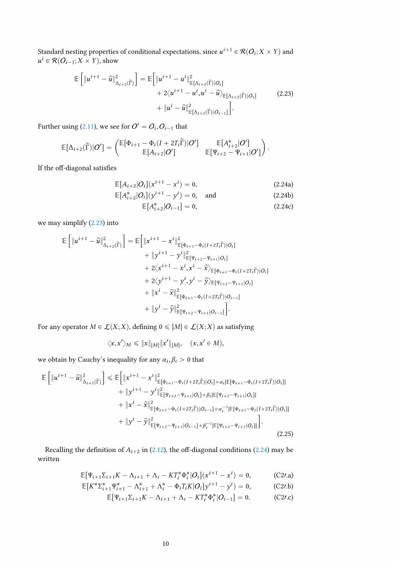
Standard nesting properties of conditional expectations, since ui`1 P RpOi ;X ˆ Y q andui P RpOi´1;X ˆ Y q, show

E”

ui`1 ´ pu2∆i`2prΓq

ı

“ E”

ui`1 ´ ui2Er∆i`2prΓq|Oi s

` 2xui`1 ´ ui ,ui ´ puyEr∆i`2prΓq|Oi s

` ui ´ pu2Er∆i`2prΓq|Oi´1s

ı

.

(2.23)

Further using (2.11), we see for O1 “ Oi ,Oi´1 that

Er∆i`2prΓq|O1s “

ˆ

ErΦi`1 ´ ΦipI ` 2TirΓq|O1s ErA˚i`2|O1s

ErAi`2|O1s ErΨi`2 ´ Ψi`1|O

1s

˙

.

If the o-diagonal satises

ErAi`2|Oi spxi`1 ´ x iq “ 0, (2.24a)

ErA˚i`2|Oi spyi`1 ´ y iq “ 0, and (2.24b)

ErA˚i`2|Oi´1s “ 0, (2.24c)

we may simplify (2.23) into

E”

ui`1 ´ pu2∆i`2prΓq

ı

“ E”

x i`1 ´ x i2ErΦi`1´Φi pI`2TirΓq|Oi s

` y i`1 ´ y i2ErΨi`2´Ψi`1|Oi s

` 2xx i`1 ´ x i ,x i ´ pxyErΦi`1´Φi pI`2TirΓq|Oi s

` 2xy i`1 ´ y i ,y i ´ pyyErΨi`2´Ψi`1|Oi s

` x i ´ px2ErΦi`1´Φi pI`2TirΓq|Oi´1s

` y i ´ py2ErΨi`2´Ψi`1|Oi´1s

ı

.

For any operator M P LpX ;X q, dening 0 ď ~M~ P LpX ;X q as satisfying

xx ,x 1yM ď x~M ~x1~M ~, px ,x 1 P Mq,

we obtain by Cauchy’s inequality for any αi ,βi ą 0 that

E”

ui`1 ´ pu2∆i`2prΓq

ı

ď E”

x i`1 ´ x i2ErΦi`1´Φi pI`2TirΓq|Oi s`αi ~ErΦi`1´Φi pI`2TirΓq|Oi s~

` y i`1 ´ y i2ErΨi`2´Ψi`1|Oi s`βi ~ErΨi`2´Ψi`1|Oi s~

` x i ´ px2ErΦi`1´Φi pI`2TirΓq|Oi´1s`α

´1i ~ErΦi`1´Φi pI`2TirΓq|Oi s~

` y i ´ py2ErΨi`2´Ψi`1|Oi´1s`β

´1i ~ErΨi`2´Ψi`1|Oi s~

ı

.

(2.25)

Recalling the denition of Ai`2 in (2.12), the o-diagonal conditions (2.24) may bewritten

ErΨi`1Σi`1K ´ Λi`1 ` Λi ´ KT ˚i Φ˚i |Oi spx

i`1 ´ x iq “ 0, (C21.a)ErK˚Σ˚i`1Ψ

˚i`1 ´ Λ˚i`1 ` Λ˚i ´ ΦiTiK |Oi sy

i`1 ´ y iq “ 0, (C21.b)ErΨi`1Σi`1K ´ Λi`1 ` Λi ´ KT ˚i Φ

˚i |Oi´1s “ 0. (C21.c)

10

Using (2.21) on the right hand side, and (2.25) on the left hand side of (C2), we see that(C2) is satised if in addition to (C21.a)–(C21.c), we have some bounds bxi`2p

rΓq,byi`2 P R

such that

E“

x i`1 ´ x i2ErΦi`1´Φi pI`2TirΓq|Oi s`αi ~ErΦi`1´Φi pI`2TirΓq|Oi s~´δΦi

` x i ´ px2ErΦi`1´Φi pI`2TirΓq|Oi´1s`α

´1i ~ErΦi`1´Φi pI`2TirΓq|Oi s~

‰

ď bxi`2prΓq, (C21.d)

and

E“

y i`1 ´ y i2ErΨi`2´Ψi`1|Oi s`βi ~ErΨi`2´Ψi`1|Oi s~

` y i ´ py2ErΨi`2´Ψi`1|Oi´1s`β

´1i ~ErΨi`2´Ψi`1|Oi s~

‰

ď byi`2. (C21.e)

The bounds bxi`2prΓq and b

yi`2 clearly exist if the iterates stay bounded, or if the con-

ditional operator expectations stay negative semi-denite. The achieve the latter, weneed to choose the testing operators Φi and Ψi suitably. We do this in the followingsections for practical block-coordinate descent algorithms. First, to conclude the presentderivations:

Corollary 2.2. We may in Corollary 2.1 replace (C1) and (C2) by (C11) and (C21).

3. Block-proximal methods

To derive practical algorithms, we need to satisfy the conditions of Corollary 2.2. To dothis, we employ ideas from the stochastic block-coordinate descent methods discussed inthe Introduction (Section 1). We construct Ti and Σi`1 to select some sub-blocks of thevariables x and y to update. This way, we also seek to gain performance improvementsthrough the local properties of G, F˚, and K .

3.1. Structure of the step length operators

Let P1, . . . ,Pm be a collection of projection operators in X , withřm

j“1 Pj “ I andPjPi “ 0 if i ‰ j. Likewise, suppose Q1, . . . ,Qn are projection operators in Y suchthat

řm`“1 Q` “ I and Q`Qk “ 0 for k ‰ `. With this, for j P t1, . . . ,nu and a subset

S Ă t1, . . . ,mu, we denote

Vpjq :“ t` P t1, . . . ,nu | Q`KPj ‰ 0u, and VpSq “ď

jPS

Vpjq.

For some tϕj,iumj“1,tψ`,i`1un`“1 Ă RpOi ; p0,8qq, we then dene

Φi :“mÿ

j“1ϕj,iPj , and Ψi`1 :“

nÿ

`“1ψ`,i`1Q` . (S-ΦΨ)

We take random subsets Spiq Ă t1, . . . ,mu, and V pi ` 1q Ă t1, . . . ,nu, deterministicwith respect to Oi , and set

Ti :“ÿ

jPSpiq

τj,iPj , and Σi`1 :“ÿ

`PV pi`1q

σ`,i`1Q` , pi ě 0q. (S-TΣ)

We assume that the blockwise step lengths satisfy tτj,i`1umj“1,tσ`,i`2u

n`“1 Ă RpOi ; p0,8qq.

Then all Φi , Ψi`1, Ti , and Σi`1 are self-adjoint and positive semi-denite.Finally, we introduce τj,i :“ τj,i χSpiqpjq and σ`,i :“ σ`,i χV piqp`q, as well as denote by

πj,i :“ Prj P Spiq | Oi´1s, and ν`,i`1 :“ Pr` P V pi ` 1q | Oi´1s,

the probability that j will be contained in Spiq and, respectively, that ` will be containedin V pi ` 1q, given what is known at iteration i ´ 1.

11

3.2. Structure of G and F˚

We assume that G and F˚ are (block-)separable in the sense

Gpxq “mÿ

j“1G jpPjxq, (S-G)

and

F˚pyq “nÿ

`“1F˚` pQ`yq. (S-F˚)

With T :“ třm

j“1 tjPj | tj ą 0u, and S :“ třn

`“1 s`Q` | s` ą 0u, the conditions (G-PM)and (F˚-PM) then reduce to the strong monotonicity of each BG j with factor γj , andthe monotonicity of each BF` . In particular (F˚-PM) is automatically satised. ThusΓ “

řmj“1 γjPj . We also write rΓ “

řmj“1 rγjPj .

Let us temporarily introduce rTi :“řm

j“1 rτj,i ě 0, satisfyingřN´1

i“0 Errτj,i s “ 1 foreach j “ 1, . . . ,m. Splitting (G-EC) into separate inequalities over all j “ 1, . . . ,m, andusing the strong convexity of G j , we see that (G-EC) holds if

G j

˜

N´1ÿ

i“0Errτj,iPjx

i`1s

¸

´G jpPjpxq ěN´1ÿ

i“0E“

rτi`

G jpxi`1q ´G jppxq

˘‰

, pj “ 1, . . . ,mq.

(3.1)The right hand side can also be written as

ş

ΩN G jpPjxipωqq ´G jpPjpxqdµ

N pi,ωq for themeasure µN :“ rτj

řN´1i“0 δi ˆ P on the domain ΩN :“ t0, . . . ,N ´ 1u ˆ Ω. Using our

assumptionřN´1

i“0 Errτj,i s “ 1, we deduce µN pΩN q “ 1. An application of Jensen’sinequality now shows (3.1). Therefore (G-EC) is automatically satised. By similararguments we see that (F˚-EC) also holds.

We now need to satisfy the conditions of Corollary 2.2 for the above structural setup.Namely, we need to satisfy (C0), (C11), and (C21) to obtain convergence estimates of theprimal iterates, and we need to satisfy either (CG) or (CG˚) to obtain gap estimates. Wedivide these verications into the following subsections Sections 3.3 to 3.6, after whichwe summarise the results in Section 3.7.

3.3. Satisfaction of the o-diagonal conditions (C21.a)–(C21.c) and either (CG) or (CG˚)

Expanded, Li`1 solved from (C0), and the proximal maps inverted, (PP) states

x i`1 “ pI `TiBGq´1px i ` Φ´1

i Λ˚i pyi`1 ´ y iq ´TiK

˚y i`1q, (3.2a)y i`1 “ pI ` Σi`1BF

˚q´1py i ` Ψ´1i`1Λipx

i`1 ´ x iq ` Σi`1Kxi`1q. (3.2b)

To derive an ecient algorithm, we have to be able to solve this system easily. Inparticular, we wish to avoid any cross-dependencies on x i`1 and y i`1 between the twosteps. One way to avoid this, is to make the rst step independent of y i`1. To do this,we could enforce Φ´1

i Λ˚i “ TiK˚, but this can be rened a little bit, as not all blocks of

y i`1 are updated.Moreover, to simplify the treatment of (C21.a) and (C21.b), and for Spiq and V pi ` 1q

to correspond exactly to the coordinates that are updated, as one would expect, weenforce

x i`1j “ x ij , pj R Spiqq, and likewise (C-cons.a)

y i`1`

“ y i` , p` R V pi ` 1qq. (C-cons.b)

12

Let us take

Λi :“mÿ

j“1

ÿ

`PVpjq

λ`,j,iQ`KPj for some λ`,j,i P RpOi , r0,8qq. (S-Λ)

If (C-cons) and (S-Λ) hold, then (C21.a)–(C21.c) follow if

Erλ`,j,i`1|Oi s “ ψ`,i`1σ`,i`1 ` λ`,j,i ´ ϕj,i τj,i ,

"

j P Spiq,` P Vpjq,

(3.3a)

Erλ`,j,i`1|Oi s “ ψ`,i`1σ`,i`1 ` λ`,j,i ´ ϕj,i τj,i ,

"

` P V pi ` 1q,j P V´1p`q,

(3.3b)

Erλ`,j,i`1|Oi´1s “ Erψ`,i`1σ`,i`1 ` λ`,j,i ´ ϕj,i τj,i |Oi´1s,

"

j “ 1, . . . ,m,` P Vpjq.

(3.3c)

We setrλ`,j,i`1 :“ ψ`,i`1σ`,i`1 ` λ`,j,i ´ ϕj,i τj,i ,

and using (3.3a) and (3.3b), compute

Erλ`,j,i`1|Oi´1s “ ErErλ`,j,i`1|Oi s|Oi´1s

“ ErErλ`,j,i`1|Oi sχV pi`1qp`q|Oi´1s

` ErErλ`,j,i`1|Oi sp1´ χV pi`1qp`qqχSpiqpjq|Oi´1s

` ErErλ`,j,i`1|Oi sp1´ χV pi`1qp`qqp1´ χSpiqpjqq|Oi´1s

“ Errλ`,j,i`1χV pi`1qp`q|Oi´1s

` Errλ`,j,i`1p1´ χV pi`1qp`qqχSpiqpjq|Oi´1s

` ErErλ`,j,i`1|Oi sp1´ χV pi`1qp`qqp1´ χSpiqpjqq|Oi´1s.

(3.4)

If

λ`,j,i “ 0, pj R Spiq or ` R V pi ` 1qq, (3.5a)

we obtain

Errλ`,j,i`1|Oi´1s “ Errλ`,j,i`1χV pi`1qp`q|Oi´1s

` Errλ`,j,i`1p1´ χV pi`1qp`qqχSpiqpjq|Oi´1s.

Together this and (3.4) show that (3.3c) holds if (3.3a) and (3.3b) do along with

ErErλ`,j,i`1|Oi sp1´ χV pi`1qp`qqp1´ χSpiqpjqq|Oi´1s “ 0.

From this, it is easy to see that (3.3) holds if (3.5a) does, and

Erλ`,j,i`1|Oi s “ ψ`,i`1σ`,i`1 ` λ`,j,i ´ ϕj,i τj,i , pj “ 1, . . . ,m; ` P Vpjqq. (3.5b)

For a specic choice of λ`,j,i , we take Spiq Ă Spiq, V pi ` 1q Ă V pi ` 1q, and set

λ`,j,i :“ ϕj,i τj,i χSpiqpjq ´ψ`,i`1σ`,i`1χV pi`1qp`q, p` P Vpjqq. (R-λ)

For λ`,j,i to take values that allow the straightforward computation of (3.2), we assume

V´1pV pi ` 1qq XV´1pVpSpiqqq “ 0. (C-nest.a)

It is then easy to see that (C-cons) and the easy computability of (3.2) demand

Spiq “ Spiq YV´1pV pi ` 1qq, and V pi ` 1q “ V pi ` 1q YVpSpiqq. (C-nest.b)

13

Assuming (C-nest) to hold, clearly the choice (R-λ) satises (3.5a), while (3.5b) followsif

Erλ`,j,i`1|Oi s “ ψ`,i`1σ`,i`1p1´ χV pi`1qp`qq ´ ϕj,i τj,ip1´ χSpiqpjqq, p` P Vpjqq.

Inserting (R-λ), we see this to be satised if for some ηi`1 P RpOi ; p0,8qq holds

Erϕj,i`1τj,i`1χSpi`1qpjq|Oi s “ ηi`1 ´ ϕj,i τj,ip1´ χSpiqpjqq ě 0, and (C-step.a)

Erψ`,i`2σ`,i`2χV pi`2qp`q|Oi s “ ηi`1 ´ψ`,i`1σ`,i`1p1´ χV pi`1qp`qq ě 0, (C-step.b)

with j “ 1, . . . ,m; ` “ 1, . . . ,n; and i ě ´1, taking

Sp´1q “ t1, . . . ,mu, and V p0q “ t1, . . . ,nu. (C-step.c)

If the testing variables ϕj,i`1 and ψ`,i`2 are known, (C-step.a) and (C-step.b) giveupdate rules for τj,i`1 andσ`,i`2 when j P Spi`1q and, respectively, ` P V pi`2q. To coverj P Spi ` 1qzSpi ` 1q and ` P V pi ` 2qzV pi ` 2q, for some ηKτ ,i`1,η

Kσ ,i`1 P RpOi ; r0,8qq,

we demand

Erϕj,i`1τj,i`1p1´ χSpi`1qpjqq|Oi s “ ηKτ ,i`1, and (C-step.d)

Erψ`,i`2σ`,i`2p1´ χV pi`2qp`qq|Oi s “ ηKσ ,i`1. (C-step.e)

Then

Erϕj,i`1τj,i`1s “ Erηi`1 ` ηKτ ,i`1 ´ ηKτ ,i s, and (3.6a)

Erψ`,i`2σ`,i`2s “ Erηi`1 ` ηKσ ,i`1 ´ ηKσ ,i s. (3.6b)

The condition (CG) is satised if Erϕj,i`1τj,i`1s “ ηi “ Erψ`,i`2σ`,i`2s. This followsif

ErηKτ ,i ´ ηKσ ,i s “ ηK :“ constant. (C-ηK)

We therefore obtain the following.

Lemma 3.1. Let us choose Λi according to (S-Λ) and (R-λ). If (C-nest), (C-step), and(C-ηK) are satised, then (C21.a)–(C21.c) and (CG) hold, as does (C-cons).

We will frequently assume for some ϵ P p0,1q that

i ÞÑ ηii ÞÑ ηKτ ,ii ÞÑ ηKσ ,i

,

.

-

are non-decreasing, and"

ϵηi ¨minjpπj,i ´ πj,iq ě ηKτ ,i ,

ηi ¨min`pν`,i`1 ´ ν`,i`1q ě ηKσ ,i .(C-η)

This ensures the non-negativity conditions in (C-step.a) and (C-step.b), while simplifyingother derivations to follow. In fact, the condition suggests to take either both ηKτ ,i andηKσ ,i as constants, or to take ηKσ ,i`1 “ ηKτ ,i “: cηi for some c ą 0 such that the non-negativity conditions in (C-step.a) and (C-step.b) are satised. Note that (C-η) guaranteesηi ě Erηi s.

If we deterministically take V pi ` 1q “ H, then (C-step.e) implies ηKσ ,i ” 0. Butthen (C-step.b) will be incompatible with (3.6b). Therefore V pi ` 1q has to be chosenrandomly to satisfy (CG). The same holds for Spiq. Thus algorithms satisfying (CG) arenecessarily doubly-stochastic, randomly updating both the primal and dual variables, orneither.

The alternative (CG˚) requires Erϕj,i`1τj,i`1s “ ηi`1 “ Erψ`,i`1σ`,i`1s. This holdswhen

Erηi`1 ` ηKτ ,i`1 ´ ηKτ ,i s “ ηi “ Erηi ` ηKσ ,i ´ ηKσ ,i´1s.

14

It does not appear possible to simultaneously satisfy this condition and the non-negativityconditions in (C-step.a) and (C-step.b) for an accelerated method, unless we deterministi-cally take V pi`1q “ H for all i . Then (C-step) and (C-nest) implyV pi`1q “ t1, . . . ,nu,Spiq “ Spiq, as well as ηKτ ,i ” 0, and ηKσ ,i`1 “ ηi . This choice satises (C-η) if i ÞÑ ηi isnon-decreasing and positive. Conversely, choosing ηKτ ,i and ηKσ ,i this way, and takingthe expectation with respect to Oi´1 in (C-step.b), we see that V pi ` 1q “ H. This saysthat to satisfy (CG˚), we need to perform full dual updates. This is akin to most existingprimal-dual coordinate descent methods [32,34,35]. The algorithms in [36–38] are moreclosely related to our method. However only [38] provides convergence rates for verylimited single-block sampling schemes under the strong assumption that both G and F˚

are strongly convex.The conditions (C-step) now reduce to

ϕj,i`1τj,i`1πj,i`1 “ ηi`1, pj “ 1, . . . ,mq, and (C-step1.a)ψ`,i`1σ`,i`1 “ ηi`1, p` “ 1, . . . ,nq. (C-step1.b)

Moreover λ`,j,i “ ϕj,i τj,i χSpiqpjq. Clearly this satises (C-cons) through (3.2). In sum-mary:

Lemma 3.2. Let us choose Λi according to (S-Λ) and (R-λ). If we ensure (C-step1), takeηKτ ,i ” 0 and ηKσ ,i`1 “ ηi , and force

Spiq “ Spiq, V pi ` 1q “ H, and V pi ` 1q “ t1, . . . ,nu,

then (C-nest) and (C-step) hold, as do (C21.a)–(C21.c), (CG˚), and (C-cons). If i ÞÑ ηi ą 0is non-decreasing, then (C-η) holds.

3.4. Satisfaction of the primal penalty bound (C21.d)

Split into blocks, the conditions asks for each j “ 1, . . . ,m the upper bound

E“

qj,i`2prγjqxi`1j ´ x ij

2 ` hj,i`2prγjqxij ´ px j

2‰ ď bxj,i`2prγjq, (3.7)

where

qj,i`2prγjq :“`

Erϕj,i`1 ´ ϕj,ip1` 2τj,irγjq|Oi s` αi |Erϕj,i`1 ´ ϕj,ip1` 2τj,irγjq|Oi s| ´ δϕj,i

˘

χSpiqpjq,(3.8)

and

hj,i`2prγjq :“ Erϕj,i`1 ´ ϕj,ip1` 2τj,irγjq|Oi´1s

` α´1i |Erϕj,i`1 ´ ϕj,ip1` 2τj,irγjq|Oi s|.

(3.9)

We easily obtain from (3.7) the following lemma.

Lemma 3.3. Suppose for some Cx ą 0 either

x i`1j ´ px j

2 ď Cx , or (C-xbnd.a)

hj,i`2prγjq ď 0 and qj,i`2prγjq ď 0, (C-xbnd.b)

for all j “ 1, . . . ,m and i P N. Then (C21.d) holds with bxi`2prΓq :“

řmj“1 b

xj,i`2prγjq for any

bxj,i`2prγjq ě 4CxErmaxt0,qj,i`2prγjqus `CxErmaxt0,hj,i`2prγjqus. (3.10)

15

Since Corollary 2.2 involve sumsřN´1

i“0 bxi`2prΓq, we dene for convenience

dxj,N prγjq :“N´1ÿ

i“0bxj,i`2prγjq. (3.11)

We still need to bound Ermaxt0,qj,i`2prγjqus and Ermaxt0,hj,i`2prγjqus. We do thisthrough primal test update rules, constructing next two possibilities.

Example 3.1 (Random primal test updates). For some constant ρ j ě 0, let us take

ϕj,i`1 :“ ϕj,ip1` 2rγj τj,iq ` 2ρ jπ´1j,i χSpiqpjq. (R-ϕrnd)

Note that ϕj,i`1 P RpOi ; p0,8qq instead of just RpOi`1; p0,8qq, as we have assumed sofar. If we set ρ j “ 0 and have just a single deterministically updated block, (R-ϕrnd) isgives the standard update rule (2.3) with the identication ϕi “ τ´2

i . The role of ρ j ą 0is to ensure some (slower) acceleration for non-strongly-convex blocks with rγj “ 0.This is necessary for convergence rate estimates.

We compute

qj,i`2prγjq “`

2p1` αiqρ jπ´1j,i ´ δϕj,i

˘

χSpiqpjq ď 2p1` αiqρ jπ´1j,i χSpiqpjq, and

(3.12a)hj,i`2prγjq “ 2ρ jπ´1

j,i ErχSpiqpjq|Oi´1s ` 2α´1i ρ jπ

´1j,i ErχSpiqpjq|Oi s. (3.12b)

This implies that (C-xbnd.b) holds if ρ j “ 0. Taking the expectation, we compute

Ermaxt0,qj,i`2prγjqus ď 2p1` αiqρ j , and (3.13a)Ermaxt0,hj,i`2prγjqus “ 2p1` α´1

i qρ j . (3.13b)

Choosing αi “ 12 and using (3.13) in (3.10), we obtain:

Lemma 3.4. If (C-xbnd.a) holds, take ρ j ě 0, otherwise take ρ j “ 0, (j “ 1, . . . ,m). If wedene ϕj,i`1 P RpOi ; p0,8qq through (R-ϕrnd), then we may take bxj,i`2prγjq “ 18Cxρ j .In particular (C21.d) holds, and dxj,N prγjq “ 18Cxρ jN .

Remark 3.1. In (R-ϕrnd), we could easily replace r j,i “ ρ jπ´1j,i χSpiqpjq by a split version

r j,i “ ρ j π´1j,i χSpiqpjq ` ρKj pπj,i ´ πj,iq

´1χSpiqzSpiqpjq without destroying the propertyErr j,i |Oi´1s “ ρ j ` ρKj “: ρ j .

The diculty with the rule (R-ϕrnd) is, as we will see in Section 4, thatηi`1 will dependon the random realisations of Spiq through ϕj,i`1. This will require communication in aparallel implementation of the algorithm. We therefore desire a deterministic updaterule for ηi`1. As we will see, this can be achieved if ϕj,i`1 is updated deterministically.

Example 3.2 (Deterministic primal test updates). Let us assume (C-step) and (C-η) tohold, and for some ρ j ě 0 and γj P r0,1qrγj take

ϕj,i`1 :“ ϕj,i ` 2pγjηi ` ρ jq. (R-ϕdet)

Since ηi P RpOi´1; p0,8qq, we see that ϕj,i`1 P RpOi´1; p0,8qq. In fact, ϕj,i`1 isdeterministic as long as ηi is chosen deterministically, for example as a function oftϕj,iu

mj“1. Since i ÞÑ ηKτ ,i is non-decreasing by (C-η), (C-step) gives

Erϕj,i τj,i |Oi´1s “ ηi ` ηKτ ,i ´ ηKi´1,τ ě ηi . (3.14)

16

Abbreviatingγj,i :“ γj`ρ jη´1i , we can writeϕj,i`1 “ ϕj,i`2γj,iηi . With this, expansion

of (3.9) gives

hj,i`2prγjq “ 2Erγj,iηi ´ rγjϕj,i τj,i |Oi´1s ` 2α´1i ~Erγj,iηi ´ rγjϕj,i τj,i |Oi s~

ď 2pγj,i ´ rγjqηi ` 2α´1i ~γj,iηi ´ rγjϕj,i τj,i ~

ď 2p1` α´1i qρ j ` 2pγj ´ rγjqηi ` 2α´1

i ~γjηi ´ rγjϕj,i τj,i ~.

Forcingα´1i ~γjηi ´ rγjϕj,i τj,i ~ ď prγj ´ γjqηi , (3.15)

and taking the expectation, this gives

Ermaxt0,hj,i`2prγjqus ď 2p1` α´1i qρ j . (3.16)

If γjηi ą rγjϕj,i τj,i , (3.15) holds when we take

αi “ αi,1 :“ minjγjprγj ´ γjq. (3.17)

Otherwise, if γjηi ď rγjϕj,i τj,i , for (3.15) to hold, we need

ϕj,i τj,i ď

ˆ

αirγj ´ γj

rγj´γj

rγj

˙

ηi . (3.18)

Taking

αi “ αi,2 :“ maxj

˜

rγj π´1j,i ´ γj

rγj ´ γj

¸

,

we see that (3.18) holds if ϕj,i τj,i ď π´1j,i ηi . We have to consider the cases j P Spiq and

j P SpiqzSpiq separately. The conditions (C-step.a) and (C-step.d) show that

ϕj,i τj,i πj,i χSpiqpjq ď ηi , and ϕj,i τj,ipπj,i ´ πj,iqp1´ χSpiqpjqq ď ηKτ ,i .

Using (C-η) in the latter estimate, we verify (3.18) (provided or not that πj,i ą 0).Next, we expand (3.8), obtaining

qj,i`2prγjq “`

2Erγj,iηi ´ rγjϕj,i τj,i |Oi s ` 2αi ~Erγj,iηi ´ rγjϕj,i τj,i |Oi s~´ δϕj,i˘

χSpiqpjq,

“`

2pγj,iηi ´ rγjϕj,i τj,iq ` 2αi ~γj,iηi ´ rγjϕj,i τj,i ~´ δϕj,i˘

χSpiqpjq,

ď`

2p1` αiqρ j ` 2pγjηi ´ rγjϕj,i τj,iq ` 2αi ~γjηi ´ rγjϕj,i τj,i ~´ δϕj,i˘

χSpiqpjq.

Again, as ηi and ϕj,iτj,i will be increasing, we want

2pγjηi ´ rγjϕj,i τj,iq ` 2αi ~γjηi ´ rγjϕj,i τj,i ~ ď δϕj,i , pj P Spiqq. (3.19)

ThenErqj,i`2prγjqs ď 2p1` αiqρ j . (3.20)

We only need to consider the case γjηi ą rγjϕj,i τj,i , as (3.19) is trivial in the oppositecase. Then αi is given by (3.17). With this the condition (3.19) expands into

rγj “ γj “ 0 or2rγjγjrγj ´ γj

ηi ď δϕj,i , pj P Spiq, i P Nq. (C-ϕdet)

In summary:

17

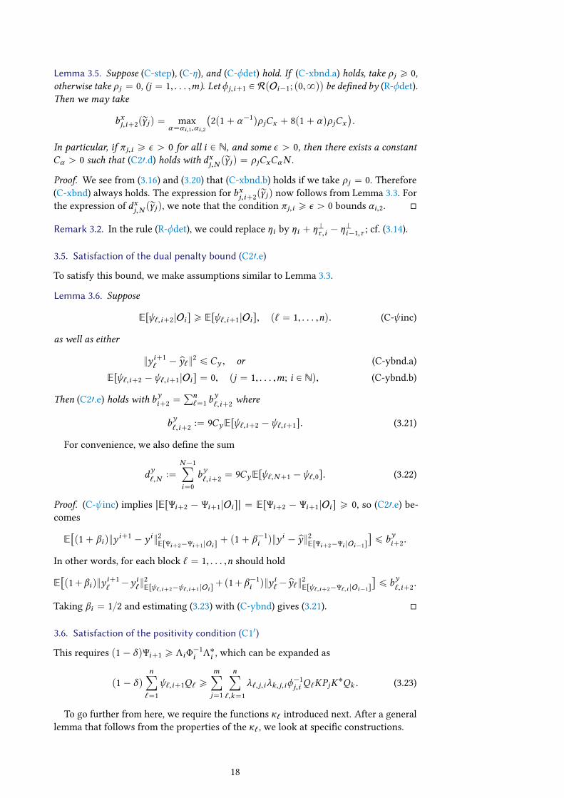
Lemma 3.5. Suppose (C-step), (C-η), and (C-ϕdet) hold. If (C-xbnd.a) holds, take ρ j ě 0,otherwise take ρ j “ 0, (j “ 1, . . . ,m). Let ϕj,i`1 P RpOi´1; p0,8qq be dened by (R-ϕdet).Then we may take

bxj,i`2prγjq “ maxα“αi,1,αi,2

`

2p1` α´1qρ jCx ` 8p1` αqρ jCx˘

.

In particular, if πj,i ě ϵ ą 0 for all i P N, and some ϵ ą 0, then there exists a constantCα ą 0 such that (C21.d) holds with dxj,N prγjq “ ρ jCxCαN .

Proof. We see from (3.16) and (3.20) that (C-xbnd.b) holds if we take ρ j “ 0. Therefore(C-xbnd) always holds. The expression for bxj,i`2prγjq now follows from Lemma 3.3. Forthe expression of dxj,N prγjq, we note that the condition πj,i ě ϵ ą 0 bounds αi,2.

Remark 3.2. In the rule (R-ϕdet), we could replace ηi by ηi ` ηKτ ,i ´ ηKi´1,τ ; cf. (3.14).

3.5. Satisfaction of the dual penalty bound (C21.e)

To satisfy this bound, we make assumptions similar to Lemma 3.3.

Lemma 3.6. Suppose

Erψ`,i`2|Oi s ě Erψ`,i`1|Oi s, p` “ 1, . . . ,nq. (C-ψ inc)

as well as either

y i`1`´ py`

2 ď Cy , or (C-ybnd.a)Erψ`,i`2 ´ψ`,i`1|Oi s “ 0, pj “ 1, . . . ,m; i P Nq, (C-ybnd.b)

Then (C21.e) holds with byi`2 “řn

`“1 by`,i`2 where

by`,i`2 :“ 9CyErψ`,i`2 ´ψ`,i`1s. (3.21)

For convenience, we also dene the sum

dy`,N :“

N´1ÿ

i“0by`,i`2 “ 9CyErψ`,N`1 ´ψ`,0s. (3.22)

Proof. (C-ψ inc) implies ~ErΨi`2 ´ Ψi`1|Oi s~ “ ErΨi`2 ´ Ψi`1|Oi s ě 0, so (C21.e) be-comes

E“

p1` βiqyi`1 ´ y i2

ErΨi`2´Ψi`1|Oi s` p1` β´1

i qyi ´ py2

ErΨi`2´Ψi |Oi´1s

‰

ď byi`2.

In other words, for each block ` “ 1, . . . ,n should hold

E“

p1`βiqy i`1`´y i`

2Erψ`,i`2´ψ`,i`1|Oi s

`p1`β´1i qy

i`´py`

2Erψ`,i`2´Ψ`,i |Oi´1s

‰

ď by`,i`2.

Taking βi “ 12 and estimating (3.23) with (C-ybnd) gives (3.21).

3.6. Satisfaction of the positivity condition (C11)

This requires p1´ δqΨi`1 ě ΛiΦ´1i Λ˚i , which can be expanded as

p1´ δqnÿ

`“1ψ`,i`1Q` ě

mÿ

j“1

nÿ

`,k“1λ`,j,iλk,j,iϕ

´1j,i Q`KPjK

˚Qk . (3.23)

To go further from here, we require the functions κ` introduced next. After a generallemma that follows from the properties of the κ` , we look at specic constructions.

18

Definition 3.1. WritingP :“ tP1, . . . ,Pmu, andQ :“ tQ1, . . . ,Qnu, we denote pκ1, . . . ,κnq PK pK ,P,Qq if each κ` : r0,8qm Ñ r0,8q, (` “ 1, . . . ,n), is monotone and we have

(i) (Estimation) The estimatemÿ

j“1

nÿ

`,k“1z

12`,j z

12k,jQ`KPjK

˚Qk ď

nÿ

`“1κ`pz`,1, . . . ,z`,mqQ` . (C-κ.a)

(ii) (Boundedness) For some κ ą 0 the bound

κ`pz1, . . . ,zmq ď κmÿ

j“1zj . (C-κ.b)

(iii) (Non-degeneracy) There exists κ ą 0 and `˚pjq P t1, . . . ,nu with

κzj˚ ď κ`˚pjqpz1, . . . ,zmq, pj P t1, . . . ,muq. (C-κ.c)

Lemma 3.7. Let pκ1, . . . ,κnq P K pK ,P,Qq. The condition (C11) then holds if

p1´ δqψ`,i`1 ě κ`p. . . ,λ2`,j,iϕ

´1j,i , . . .q, p` “ 1, . . . ,nq. (C-κψ )

Proof. Clearly Φi`1 is self-adjoint and positive denite. The remaining condition in(C11) is equivalent to (3.23), which follows from (C-κ.a) with z`,j :“ λ2

`,j,iϕ´1j,i .

Example 3.3 (Simple structural κ). Using Cauchy’s inequality, we deducenÿ

`,k“1z

12`,j z

12k,jQ`KPjK

˚Qk ď

nÿ

`“1z`,ja`,jQ` , pj “ 1, . . . ,mq, (3.24)

for a`,j :“ Q`KPj2 ¨ #Vpjq. Thus (C-κ.a) and (C-κ.b) hold with κ “ max`,j a`,j if we

take

κ`pz1, . . . ,zmq :“mÿ

j“1zja`,j .

Clearly κ` is also monotone. If minj #Vpjq ą 0, then also (C-κ.c) is satised withκ “ minj max`PVpjq a`,j ą 0 and `˚pjq :“ arg min`PVpjq a`,j .

Example 3.4 (Worst-case κ). If #Vpjq is generally large, the previous example mayprovide very poor estimates. In this case, we may alternatively proceed with z` :“maxj zj,` as follows:

mÿ

j“1

nÿ

`,k“1z

12`,j z

12k,jQ`KPjK

˚Qk ď

nÿ

`,k“1z

12`z

12k Q`KK

˚Qk ď

nÿ

`“1z`K

2Q` .

Therefore (C-κ.a) and (C-κ.b) hold with κ “ K2 for the monotone choice

κ`pz1, . . . ,zmq :“ K2 maxtz1, . . . ,zmu.

Clearly also κ “ κ for any choice of `˚pjq P t1, . . . ,nu.

Example 3.5 (Balanced κ). One more option is to choose the minimal κ` satisfying(C-κ.a) and the balancing condition

κ`pz`,1, . . . ,z`,mq “ κk pzk,1, . . . ,zk,mq, p`,k “ 1, . . . ,nq.

This involves more rened use of Cauchy’s inequality than the rough estimate (3.24),but tends to perform very well, as we will see in Section 5. This rule uses the data tz`,munon-linearly.

19

3.7. Summary so far

We now summarise our ndings so far, starting with writing out the proximal pointiteration (PP) explicitly in terms of blocks. We already reformulated it in (3.2). Wecontinue from there, rst writing the λ`,j,i from (R-λ) in operator form as

Λi “ KT ˚i Φ˚i ´ Ψi`1Σi`1K ,

where Ti :“řm

j“1 χSpiqpjqτj,iPj , and Ψi`1 :“ř`

j“1 χV pi`1qp`qσ`,iQ` . Also deningTKi :“ Ti ´Ti , and ΣKi`1 :“ Σi`1´ Σi`1, we can therefore rewrite (3.2) non-sequentiallyas

vi`1 :“ Φ´1i K˚Σ˚i`1Ψ

˚i`1py

i`1 ´ y iq `TKi K˚y i`1, (3.25a)

x i`1 :“ pI `TiBGq´1px i ´ TiK

˚y i ´vi`1q, (3.25b)

zi`1 :“ Ψ´1i`1KT

˚i Φ

˚i px

i`1 ´ x iq ` ΣKi`1Kxi`1, (3.25c)

y i`1 :“ pI ` Σi`1BF˚q´1py i ` Σi`1Kx

i ` zi`1q. (3.25d)

Let us set

Θi :“ÿ

jPSpiq

ÿ

`PVpjq

θ`,j,iQ`KPj with θ`,j,i`1 :“τj,iϕj,i

σ`,i`1ψ`,i`1.

Then thanks to (C-nest), we have ΣKi`1Θi`1 “ Ψ´1i`1KT

˚i Φ

˚i . Likewise,

Bi :“ÿ

`PV pi`1q

ÿ

jPV´1p`q

b`,j,iQ`KPj with b`,j,i`1 :“σ`,i`1ψ`,i`1

τj,iϕj,i,

satises TKi B˚i`1 “ Φ´1i K˚Σi`1Ψi`1. Now we can rewrite (3.25) as

vi`1 :“ TKi rB˚i`1py

i`1 ´ y iq ` K˚y i`1s, (3.26a)

x i`1 :“ pI `TiBGq´1px i ´ TiK

˚y i ´vi`1q, (3.26b)

zi`1 :“ ΣKi`1rΘi`1pxi`1 ´ x iq ` Kx i`1s, (3.26c)

y i`1 :“ pI ` Σi`1BF˚q´1py i ` Σi`1Kx

i ` zi`1q. (3.26d)

Observe how (3.26b) can thanks to (S-G) be split into separate steps with respect to TiandTKi , while (C-nest.a) guarantees zi`1 “ ΣKi`1rΘi`1px

i`1 ´ x iq `Kx i`1s. Therefore,we obtain

x i`1 :“ pI ` TiBGq´1px i ´ TiK

˚y iq, (3.27a)w i`1 :“ Θi`1px

i`1 ´ x iq ` x i`1, (3.27b)

y i`1 :“ pI ` Σi`1BF˚q´1py i ` Σi`1Kx

i ` ΣKi`1wi`1q, (3.27c)

vi`1 :“ B˚i`1pyi`1 ´ y iq ` y i`1, (3.27d)

x i`1 :“ pI `TKi BGq´1px i`1 ´TKi v

i`1q. (3.27e)

In the blockwise case under consideration, in particular the setup of Lemma 3.1together with (S-G) and (S-F˚), the iterations (3.27) easily reduce to Algorithm 1. Therewe write

x j :“ Pjx , y` :“ Q`y , and K`,j :“ Q`KPj .

In particular (C-step.a) can be written

ϕj,i`1Erτj,i`1|j P Spi ` 1qsπj,i`1 “ ηi`1 ´ ϕj,i τj,ip1´ χSpiqpjqq.

20

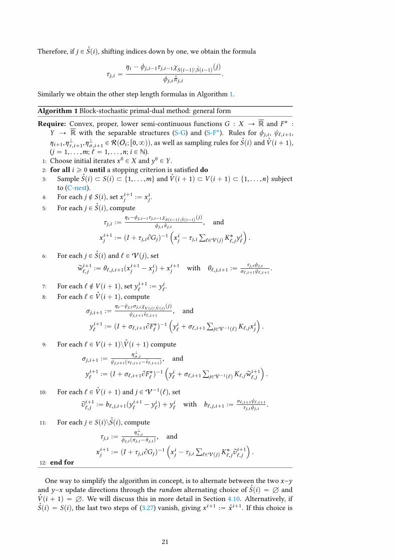
Therefore, if j P Spiq, shifting indices down by one, we obtain the formula

τj,i “ηi ´ ϕj,i´1τj,i´1χSpi´1qzSpi´1qpjq

ϕj,i πj,i.

Similarly we obtain the other step length formulas in Algorithm 1.

Algorithm 1 Block-stochastic primal-dual method: general form

Require: Convex, proper, lower semi-continuous functions G : X Ñ R and F˚ :Y Ñ R with the separable structures (S-G) and (S-F˚). Rules for ϕj,i , ψ`,i`1,ηi`1,η

Kτ ,i`1,η

Kσ ,i`1 P RpOi ; r0,8qq, as well as sampling rules for Spiq and V pi ` 1q,

(j “ 1, . . . ,m; ` “ 1, . . . ,n; i P N).1: Choose initial iterates x0 P X and y0 P Y .2: for all i ě 0 until a stopping criterion is satised do3: Sample Spiq Ă Spiq Ă t1, . . . ,mu and V pi ` 1q Ă V pi ` 1q Ă t1, . . . ,nu subject

to (C-nest).4: For each j R Spiq, set x i`1

j :“ x ij .5: For each j P Spiq, compute

τj,i :“ηi´ϕj,i´1τj,i´1χSpi´1qzSpi´1qpjq

ϕj,i πj,i, and

x i`1j :“ pI ` τj,iBG jq

´1´

x ij ´ τj,iř

`PVpjq K˚`,jy

i`

¯

.

6: For each j P Spiq and ` P Vpjq, set

rw i`1`,j :“ θ`,j,i`1px

i`1j ´ x ij q ` x i`1

j with θ`,j,i`1 :“ τj,iϕj,iσ`,i`1ψ`,i`1

.

7: For each ` R V pi ` 1q, set y i`1`

:“ y i`.

8: For each ` P V pi ` 1q, compute

σj,i`1 :“ηi´ψj,iσj,i χV piqzV piqpjq

ψj,i`1ν`,i`1, and

y i`1`

:“ pI ` σ`,i`1BF˚`q´1

´

y i`` σ`,i`1

ř

jPV´1p`q K`,jxij

¯

.

9: For each ` P V pi ` 1qzV pi ` 1q compute

σj,i`1 :“ηKσ ,i

ψj,i`1pν`,i`1´ν`,i`1q, and

y i`1`

:“ pI ` σ`,i`1BF˚`q´1

´

y i`` σ`,i`1

ř

jPV´1p`q K`,j rwi`1`,j

¯

.

10: For each ` P V pi ` 1q and j P V´1p`q, set

rvi`1`,j :“ b`,j,i`1py

i`1`´ y i

`q ` y i

`with b`,j,i`1 :“ σ`,i`1ψ`,i`1

τj,iϕj,i.

11: For each j P SpiqzSpiq, compute

τj,i :“ηKτ ,i

ϕj,i pπj,i´πj,i q, and

x i`1j :“ pI ` τj,iBG jq

´1´

x ij ´ τj,iř

`PVpjq K˚`,j rv

i`1`,j

¯

.

12: end for

One way to simplify the algorithm in concept, is to alternate between the two x–yand y–x update directions through the random alternating choice of Spiq “ H andV pi ` 1q “ H. We will discuss this in more detail in Section 4.10. Alternatively, ifSpiq “ Spiq, the last two steps of (3.27) vanish, giving x i`1 :“ x i`1. If this choice is

21

deterministic, then also V pi ` 1q “ H, so we are in the full dual updates setting ofLemma 3.2. The result is Algorithm 2.

Algorithm 2 Block-stochastic primal-dual method: full dual updates

Require: Convex, proper, lower semi-continuous functions G : X Ñ R and F˚ :Y Ñ R with the separable structures (S-G) and (S-F˚). Rules for ϕj,i ,ψ`,i`1,ηi`1 P

RpOi ; p0,8qq, as well as a sampling rule for the set Spiq, (j “ 1, . . . ,m; ` “ 1, . . . ,n;i P N).

1: Choose initial iterates x0 P X and y0 P Y .2: for all i ě 0 until a stopping criterion is satised do3: Select random Spiq Ă t1, . . . ,mu.4: For each j R Spiq, set x i`1

j :“ x ij .5: For each j P Spiq, with τj,i :“ ηiπ

´1j,i ϕ

´1j,i , compute

x i`1j :“ pI ` τj,iBG jq

´1´

x ij ´ τj,iř

`PVpjq K˚`,jy

i`

¯

.

6: For each j P Spiq set

x i`1j :“ θ j,i`1px

i`1j ´ x ij q ` x i`1

j with θ j,i`1 :“ηi

πj,iηi`1.

7: For each ` P t1, . . . ,nu using σ`,i`1 :“ ηi`1ψ´1`,i`1, compute

y i`1`

:“ pI ` σ`,i`1BF˚`q´1

´

y i`` σ`,i`1

ř

jPV´1p`q K`,j xi`1j

¯

.

8: end for

We have not yet specied ηi andψ`,i . We have also not xed ϕj,i , giving the optionsin Example 3.1 and Example 3.2. We will return to these choices in the next section, butnow summarise our results so far by specialising Corollary 2.2.

Proposition 3.1. Let δ P p0,1q and pκ1, . . . ,κnq P K pK ,P,Qq. Then the conditions (C0),(C11), and (C21) hold when we do the following for each i P N.

(i) Sample Spiq Ă Spiq Ă t1, . . . ,mu and V pi ` 1q Ă V pi ` 1q Ă t1, . . . ,nu subject to(C-nest).

(ii) Dene Φi`1 through (S-ΦΨ), satisfying (C-xbnd) for rγj ě 0 to be specied.

(iii) Dene Ψi`1 through (S-ΦΨ), satisfying (C-ψ inc), (C-ybnd), and (C-κψ ).

(iv) TakeTi and Σi of the form (S-TΣ) with the blockwise step lengths satisfying (C-step).

(v) Dene Λi through (S-Λ) and (R-λ).

(vi) Either (Lemma 3.1 or Lemma 3.2)

(a) Take ηKτ ,i and ηKσ ,i satisfying (C-ηK) and (C-step). In this case (CG) holds; or

(b) Satisfy (C-step1), forcing Spiq “ Spiq, V pi ` 1q “ H, V pi ` 1q “ t1, . . . ,nu.In this case (CG˚) holds, as do (C-nest) and (C-step) with ηKτ ,i ” 0, andηKσ ,i`1 “ ηi .

Let thenG and F˚ have the separable structures (S-G) and (S-F˚). For each j “ 1, . . . ,m,suppose G j is (strongly) convex with corresponding factor γj ě 0, and pick rγj P r0,γj s.Then there exists C0 ą 0 such that the iterates of (PP) satisfy

δmÿ

k“1

1Erϕ´1

k,N s¨ E

“

xNk ´ pxk‰2` rдN ď C0 `

mÿ

j“1dxj,N prγjq `

nÿ

`“1dy`,N , (3.30)

22

where dxj,N prγjq is dened in (3.11), dy`,N is dened in (3.22), and we set

rдN :“

$

’

&

’

%

ζNGprxN ,ryN q, (CG) holds and rγj ď γj2 for all j,ζ ,NGprx ,N ,ry ,N q, (CG˚) holds and rγj ď γj2 for all j,0, otherwise.

Here ζN and the ergodic variables rxN and ryN in (2.15), and the gap G in (2.16). Thealternatives ζ ,N , rx ,N and ry ,N are dened in (2.19).

Proof. We have proved all of the conditions (C0), (C11), (C21) and (CG), alternatively(CG˚), in Lemmas 3.1 to 3.3, 3.6 and 3.7. Only the estimate (3.30) demands furtherverication.

In Corollary 2.2, we have assumed that either rΓ “ Γ or rΓ “ Γ2, that is rγj P tγj ,γj2u.However, G j is (strongly) convex with factor γ 1j for any γ 1j P r0,γj s, so we may relax thisassumption to 0 ď rγj ď γj with the gap estimates holding when rγj ď γj2.

Setting C0 :“ 12u

0 ´ pu2Z0L0, Corollary 2.2 thus shows

δErxN ´ px2ΦN s ` rдN ď C0 `

N´1ÿ

i“0pbxi`2prγjq ` b

yi`2q.

By Hölder’s inequality

ErxN ´ px2ΦN s “mÿ

k“1E“

ϕk,N xNk ´ pxk

2‰ ě

mÿ

k“1ErxNk ´ pxks

2Erϕ´1k,N s.

The estimate (3.30) is now immediate.

Specialised to Algorithms 1 and 2, we obtain the following corollaries.

Corollary 3.1. Let δ P p0,1q and pκ1, . . . ,κnq P K pK ,P,Qq. Suppose the primal bound(C-xbnd), and the dual test conditions (C-ψ inc), (C-ybnd), and (C-κψ ) hold along with(C-ηK), (C-η). Then the iterates of Algorithm 1 satisfy (3.30) with rдN “ ζNGprxN ,ryN qwhen rγj ď γj2 for all j, and rдN “ 0 otherwise.

Proof. Algorithm 1 satises the structural assumptions (S-ΦΨ), (S-TΣ), and (S-Λ), theconditions (C-nest) and (R-λ), as well as the alternative condition (a) of Proposition 3.1,provided the non-negativity conditions in (C-step) are satised. They are indeed ensuredby us assuming (C-η). The remaining conditions of Proposition 3.1 we have also assumed.

Corollary 3.2. Let δ P p0,1q and pκ1, . . . ,κnq P K pK ,P,Qq. Suppose (C-xbnd) and thedual conditions (C-ψ inc), (C-ybnd), and (C-κψ ) hold. Then the iterates of Algorithm 2satisfy (3.30)with rдN “ ζ ,NGprx ,N ,ry ,N qwhen rγj ď γj2 for all j , and rдN “ 0 otherwise.

Proof. Algorithm 2 satises the structural assumptions (S-ΦΨ), (S-TΣ), (S-Λ) and (R-λ),as well as (b) of Proposition 3.1. Its remaining conditions we have assumed.

4. Dual tests and penalty bounds for block-proximal methods

We now need to satisfy the conditions of Corollaries 3.1 and 3.2. This involves choosingupdate rules for ηi`1, ηKτ ,i`1, ηKσ ,i`1, ϕj,i`1 andψ`,i`1. Specically, for both Corollaries,we have to verify the primal bound (C-xbnd). For Corollary 3.1, we moreover need(C-ηK), (C-η), and the non-negativity conditions in (C-step.a) and (C-step.b). At the

23

same time, to obtain good convergence rates, we need to make dxj,N prγjq and dy`,N “

Erψ`,N`1 ´ψ`,0s small in (3.30).We concentrate on the deterministic primal test update rule of Example 3.2, which

also provide estimates on dxj,N prγjq if the conditions of 3.5 are satised. In addition tothe verications above, we need to verify (C-ϕdet). To satisfy (C-xbnd), we have to takeρ j “ 0 unless the bound (C-xbnd.a) holds for the specic problem under consideration.

We begin with general assumptions, after which in Section 4.2 we calculate expectationbounds on ϕj,i . In Sections 4.3 to 4.8 we give useful choice of ηi and ψ`,i that nallyyield specic convergence results. We nish the section with choices for ηKτ ,i and ηKσ ,i inSection 4.9, and sampling patterns in Section 4.10. The diculty of (fully) extending ourestimates to the random primal test update of Example 3.1, we discuss in Remark 4.2.

4.1. Assumptions and simplifications

Throughout this section, we assume for simplicity that the probabilities stay constantbetween iterations,

πj,i ” πj ą 0, and ν`,i ” ν` . (R-πν )

Then (C-nest) shows that

πj,i ” πj ą 0, and ν`,i ” ν` ą 0.

We assume (C-η) to hold. As we recall from Lemma 3.2, this is the case for Algorithm 2if

i ÞÑ ηi ą 0 is non-decreasing.

Finally, aside from the non-negativity conditions that will be veried through thechoice of ηKτ ,i and ηKσ ,i , we note that (C-step) holds in Algorithms 1 and 2. It is thereforeassumed.

4.2. Estimates for deterministic primal test updates

We consider the deterministic primal test updates of Example 3.2. To start with, from(R-ϕdet), we compute

ϕj,N “ ϕj,N´1 ` 2pγjηN´1 ` ρ jq “ ϕj,0 ` 2ρ jN ` 2γjN´1ÿ

i“0ηi . (4.1)

The following lemma lists the fundamental properties that this update rule satises.

Lemma 4.1. Suppose (C-η), (C-ϕdet), and (R-πν ) hold. If (C-xbnd.a) holds with theconstantCx ě 0, take ρ j ě 0, otherwise take ρ j “ 0, supposing rγj`ρ j ą 0, (j “ 1, . . . ,m).Dene ϕj,i`1 according to Example 3.2. Suppose ηi ě bjpi ` 1qp , for some p,bj ą 0. Thenfor some c j ą 0, and Cα ą 0 holds

ϕj,N P RpON´1; p0,8qq, (C-ϕbnd.a)

Erϕj,N s “ ϕj,0 ` 2ρ jN ` 2γjN´1ÿ

i“0Erηi s, and (C-ϕbnd.b)

Erϕ´1j,N s ď c jN

´1, pN ě 1q. (C-ϕbnd.c)

Moreover, the primal test bound (C-xbnd) holds, and with Cα “ 18 we have

dxj,N prγjq “ ρ jCxCαN . (C-ϕbnd.d)

24

Suppose moreover that ηi ě bj minj ϕpj,i , for some p,bj ą 0. Then for some rc j ě 0 holds

1Erϕ´1

j,N sě γjrc jN

p`1, pN ě 4q. (C-ϕbnd.e)

Proof. The conditions of Lemma 3.5 are guaranteed by our assumptions. It directlyproves (C-ϕbnd.a) and (C-ϕbnd.d). Since we assume i ÞÑ ηi to be increasing, clearlyϕj,N ě 2N rρ j for rρ j :“ ρ j ` γjη0 ą 0. Then ϕ´1

j,N ď1

2rρ jN . Taking the expectation proves(C-ϕbnd.c), while (C-ϕbnd.b) is immediate from (4.1). Clearly (C-ϕbnd.e) holds if γj “ 0,so assume γj ą 0. Under our assumption on ηi , Lemma B.1 shows for some Bj ą 0 thatϕ´1j,N ď

1BjN 1`p . Taking the expectation proves (C-ϕbnd.e) for a rc j :“ Bjγj .

Remark 4.1. From (4.1), we see that ηi ě bjpi ` 1qp if ηi ě rbj minj ϕpj,i for some rbj ą 0.

Remark 4.2. Propositions 4.1 and 4.2 to follow, will generalise to any update rulefor ϕj,i`1 that satises (C-ϕbnd). The conditions (C-ϕbnd.a)–(C-ϕbnd.d) can easily beshown for the random primal test updates of Example 3.1. The estimate (C-ϕbnd.e)however is challenging, with any derivation likely dependent on the exact samplingpatterns employed. The estimate (C-ϕbnd.e) is, however, only needed to estimate1Erϕ´1

j,N s from below in the rst term of the general estimate (3.30), and therefore onlyaects convergence of the iterates, not the gap. Hence the estimates in the upcomingPropositions 4.1 and 4.2 on the ergodic duality gap, but not the iterates, do hold for therandom primal test update rule of Example 3.1.

4.3. Dual bounds—a first aempt

We now need to satisfy the conditions (C-ψ inc), (C-ybnd), and (C-κψ ) on the dualupdates. By the construction of λ`,j,i in (R-λ), the step length condition (C-step), andthe constant probability assumption (R-πν ), we have

λl,j,i ď ηi`

π´1j χSpiqpjq ` ν´1

`χV pi`1qp`q

˘

“: ηi µ`,j,i , p` P Vpjqq.

Therefore (C-κψ ) holds if we take

ψ`,i`1 :“η2i

1´ δκ`p. . . , µ

2`,j,iϕ

´1j,i , . . .q. (4.2)

With this, the condition (C-ψ inc) would require for all ` “ 1, . . . ,n that

Erη2i`1κ`p. . . , µ

2`,j,i`1ϕ

´1j,i`1, . . .q|Oi s ě Erη2

iκ`p. . . , µ2`,j,iϕ

´1j,i , . . .q|Oi s (4.3)

Since ηi`1 P RpOi ; p0,8qq, and ηi P RpOi ; p0,8qq, we can take ηi and ηi`1 outside theexpectations in (4.3). A rst idea would then be to take ηi`1 as the smallest numbersatisfying (4.3) for all `. In the deterministic case, the resulting rule will telescope, andreduce to the one that we will follow. In the stochastic case, we have however observednumerical instability, and have also been unable to prove convergence. Therefore, wehave to study “less optimal” rules.

4.4. Worst-case conditions

For a random variable p P RpΩ;Rq on the probability space pΩ,O,Pq, let us dene theconditional worst-case realisation with respect to the σ -algebra O1 Ă O as the randomvariable Wrp|O1s P RpO1;Rq dened by

p ď Wrp|O1s ď q P-a.e. for all q P RpO1;Rq s.t. p ď q P-a.e.

25

We also write Wrps :“ Wrp|O1s when O1 “ tΩ,Hu is the trivial σ -algebra.Following the derivation of (4.2), the condition (C-κψ ) will hold if

ψ`,i`1 ěη2i

1´ δWrκ`p. . . , µ

2`,j,iϕ

´1j,i , . . .q|Oi´1s. (4.4)

Accordingly, we take

ηi :“ min`“1, ...,n

g

f

f

e

p1´ δqψ`,i`1

Wrκ`p. . . , µ2`,j,iϕ

´1j,i , . . .q|Oi´1s

. (R-η)

By the construction ofW, we getηi P RpOi´1; p0,8qq provided alsoψi`1 P RpOi´1; p0,8qq.It is our task in the rest of this section to experiment with dierent choices of ψ`,i`1,satisfying (C-ψ inc) and (C-ybnd). Before this we establish the following important fact.

Lemma 4.2. Let δ P p0,1q and pκ1, . . . ,κnq P K pK ,P,Qq. Suppose (R-πν ) holds, and thatboth i ÞÑ ϕj,i and i ÞÑ ψ`,i are non-decreasing for all j “ 1, . . . ,m and ` “ 1, . . . ,n. Theni ÞÑ ηi dened in (R-η) is non-decreasing.

Proof. We x ` P t1, . . . ,nu. The condition (R-πν ) implies that pµ`,1,i , . . . , µ`,m,iq areindependently identically distributed for all i P N. Since ϕj,i P RpOi´1; p0,8qq, wecan for some random pµ1, . . . , µmq on a probability space pPµ ,Ωµ ,Oµq, distinct frompP,Ω,Oq, write

Wrκ`p. . . , µ2`,j,iϕ

´1j,i , . . .q|Oi´1s „ Wrκ`p. . . , µ

2jϕ´1j,i , . . .qs, pi P Nq,

where „ stands for “identically distributed”. Since i ÞÑ ϕj,i is non-decreasing and κ`monotone, this implies

Wrκ`p. . . , µ2`,j,iϕ

´1j,i , . . .q|Oi´1s ě Wrκ`p. . . , µ

2`,j,i`1ϕ

´1j,i`1, . . .q|Oi s, P-a.e.

Since i ÞÑ ψ`,i is also non-decreasing, the claim follows.

4.5. Partial strong convexity: Boundedψ

In addition to the assumptions in Section 4.1, from now on we assume (C-ϕbnd) to hold.As we have seen, this is the case for the deterministic primal test update rule of bothExample 3.2. For the random primal test update rule of (3.1), the rest of the conditionshold, but we have not been able to verify (C-ϕbnd.e). This has the implication that onlythe gap estimates hold.

As a rst option forψ`,i , let us takeψ`,i ” ψ`,0. Then both (C-ψ inc) and (C-ybnd.b)clearly hold, and d

y`,N ” 0. Moreover Lemma 4.2 shows that i ÞÑ ηi is non-decreasing,

as we have required in Section 4.1. To obtain convergence rates, we still need toestimate the primal penalty dxj,N prγjq as well as ζN and ζ ,N . Presently the dual penaltydy`,N “ Erψ`,N ´ψ`,0s ” 0.

Withψ0

:“ min`“1, ...,nψ`,0, we compute

ηi ě

g

f

f

e

p1´ δqψ0

max`“1, ...,n Wrκ`p. . . , µ2`,j,iϕ

´1j,i , . . .q|Oi´1s

.

Let us dene

wj :“ max`PVpjq

Wrµ`,j,i |Oi´1s “ max`PVpjq

W“

π´1j χSpiqpjq ` ν´1

`χV pi`1qp`q

ˇ

ˇ Oi´1‰

,

26

which is independent of i ě 0; see the proof of Lemma 4.2. Since µ`,j,i “ 0 for ` R Vpjq,using (C-κ.b) and ϕj,i P RpOi´1; p0,8qq, we further get

ηi ě

g

f

f

e

p1´ δqψ0

κ max`PVpjqWrřn

j“1 µ2`,j,iϕ

´1j,i |Oi´1s

ě

d

1řn

j“1 b´1j ϕ´1

j,i

(4.5)

for bj :“ p1´ δqψ0pκw2j q. Jensen’s inequality thus gives

Erηi s ě´

E”b

řnj“1 b

´1j ϕ´1

j,i

ı¯´1ě

´

řnj“1 b

´1j Erϕ´1

j,i s

¯´12. (4.6)

Using (C-ϕbnd.c), it follows

Erηi s ě Cηi12 for Cη :“

´

řmj“1 b

´1j c j

¯´12. (4.7)

We recall (C-η) guaranteeing ηi ě Erηi s. Consequently, we estimate ζN from (2.14)by

ζN “N´1ÿ

i“0ηi ě

N´1ÿ

i“0Erηi s ě Cη

N´1ÿ

i“0i12 ě Cη

ż N´2

0x12 dx ě

2Cη3pN ´ 2q32

“2Cη

3N 32

ˆ

N ´ 2N

˙32“

Cη?

18N 32, pN ě 4q.

(4.8)

Similarly ζ ,N dened in (2.18) satises

ζ ,N ě

N´1ÿ

i“1Erηi s ě

2Cη3ppN´2q32´1q ě

p232 ´ 1qCη232

?18

N 32 ěCη

2?

18N 32, pN ě 4q.

(4.9)For the deterministic primal test update rule of Example 3.2, by Lemma 3.5, we still

need to satisfy (C-ϕdet), that is 2rγjγjηi ď δϕj,iprγj ´ γjq for j P Spiq and i P N. Thenon-degeneracy assumption (C-κ.c) applied in (R-η) gives ηi ď

a

p1´ δqψ`,0ϕj,ipκwjq.Since under both rules Examples 3.1 and 3.2, ϕj,i is increasing in i , it therefore sucesto choose γj ě 0 to satisfy

rγj “ γj “ 0 or2rγjγjrγj ´ γj

d

1´ δ

κwjď δψ

´12`,0 ϕ

12j,0 . (C-ϕdet1)

These ndings can be summarised as:

Proposition 4.1. Let δ P p0,1q and pκ1, . . . ,κnq P K pK ,P,Qq. Pick ρ j ě 0 and rγj P r0,γj s,(j “ 1, . . . ,m). In Algorithm 1 or Algorithm 2, take

(i) the probabilities πj,i ” πj and (in Algorithm 1) ν`,i ” ν` constant over iterations,

(ii) ηi according to (R-η), and (in Algorithm 1) ηKτ ,i ,ηKσ ,i ą 0 satisfying (C-η) and (C-ηK),

(iii) ϕj,0 ą 0 by free choice, and ϕj,i for i ě 1 following Example 3.2, taking 0 ď γj ă rγjor γj “ 0, and satisfying (C-ϕdet1),

(iv) ψ`,i :“ ψ`,0 for some xedψ`,0 ą 0, (` “ 1, . . . ,n).

27

Suppose for each j “ 1, . . . ,m that ρ j ` γj ą 0 and either ρ j “ 0 or (C-xbnd.a) holds withthe constant Cx . Let rck be the constant provided by Lemma 4.1. Then

mÿ

k“1δrckγkE

“

xNk ´ pxk‰2`

Cη?

18дN ď

C0 `CxCα přm

j“1 ρ jqN

N 32, pN ě 4q, (4.10)

where

дN :“

$

’

&

’

%

GprxN ,ryN q, Algorithm 1, rγj ď γj2 for all j,12Gprx ,N ,ry ,N q, Algorithm 2, rγj ď γj2 for all j,0, otherwise.

Proof. By (4.5), we have ηi ě b12j minj ϕ

12j,i for each j “ 1, . . . ,m, so (C-ϕbnd.e) holds

with p “ 12. Therefore, (4.10) is immediate from (C-ϕbnd.e), Corollaries 3.1 and 3.2,and the estimates (4.8) and (4.9), whose assumptions follow from Lemmas 4.1 and 4.2and (C-ϕdet1).

Remark 4.3 (Practical parameter initialisation). In practise, we take τj,0, ηi , and δ Pp0,1q as the free step length parameters. Then (C-step.a) and (C-step.b) give ϕj,0 “η0pτj,0πj,0q. As ψ`,0 we take a value reaching the maximum in (R-η). In practise, wetake η0 “ 1minj τj,0. This choice appears to work well, and is consistent with the basicalgorithm (2.2) corresponding to ϕj,0 “ τ´2

j,0 . For the deterministic update rule (R-ϕdet),we use (C-ϕdet1) to bound γj .

4.6. Partial strong convexity: Increasingψ

In (R-η), let us takeψ`,i`1 :“ ψ`,0ηi . Then

ηi “ min`“1, ...,n

p1´ δqψ`,0

Wrκ`p. . . , µ2`,j,iϕ

´1j,i , . . .q|Oi´1s

. (R-η2)

Adapting Lemma 4.2, we see that i ÞÑ ηi is non-decreasing. Thus i ÞÑ ψ`,i is also in-creasing, so (C-ψ inc) holds. As (C-ybnd.b) does not hold, we need to assume (C-ybnd.a).To obtain convergence rates, we need to estimate both the primal and the dual penaltiesdxj,N prγjq and d

y`,N , as well as ζN and Erψk,N s.

Similarly to the derivation of (4.7), we deduce with the help of (C-ϕbnd.c) that

Erηi s ě C2ηi . (4.11)

Consequently

ζN “N´1ÿ

i“0ηi ě

N´1ÿ

i“0Erηi s ě C2

η

N´1ÿ

i“0i ě C2

η

ż N´2

0x dx ě

C2η

2pN ´ 2q2

“C2η

2N 2

ˆ

N ´ 2N

˙2ě

C2η

8N 2, pN ě 4q.

(4.12)

Similarly

ζ ,N ě

N´1ÿ

i“1Erηi s ě

C2η

2ppN ´ 2q2 ´ 1q “

34C

2η

8N 2, pN ě 4q. (4.13)

We still need to boundψ`,N`1 to bound dy`,N . To do this, we assume the existence of

some j˚ with γj˚ “ 0. With the help (C-κ.c), we then deduce from (R-η2) that

ηi ďp1´ δqψ`˚pj˚q,0

κw2`˚pj˚q

ϕj˚,i .

28

Since γj˚ “ 0, a referral to (C-ϕbnd.b) shows that

Erϕj˚,N s “ ϕj˚,0 ` N ρ j˚ .

Consequently

ErdNy ,`s “ ψ`,0pErηN s´1q ď ψ`,0

˜

p1´ δqψ`˚pj˚q,0

κw2j˚

Erϕj˚,N s ´ 1

¸

ď ψ`,0`

Cη,˚N`δ˚˘

(4.14)for

Cη,˚ :“p1´ δqψ`˚pj˚q,0ρ j˚

κwj˚and δ˚ :“

p1´ δqψ`˚pj˚q,0ϕj˚,0

κwj˚´ 1. (4.15)

For the deterministic primal test update rule of Example 3.2, we still need to satisfy(C-ϕdet). Similarly to the derivation of (C-ϕdet1), we obtain for γj ě 0 the condition

rγj “ γj “ 0 or2rγjγjrγj ´ γj

p1´ δqψ`,0

κwjď δ , p` P Vpjqq. (C-ϕdet2)

In summary:

Proposition 4.2. Let δ P p0,1q and pκ1, . . . ,κnq P K pK ,P,Qq. Pick ρ j ě 0 and rγj P r0,γj s,(j “ 1, . . . ,m). In Algorithm 1 or Algorithm 2, take

(i) the probabilities πj,i ” πj and (in Algorithm 1) ν`,i ” ν` constant over iterations,

(ii) ηi according to (R-η2), and (in Algorithm 1) ηKτ ,i ,ηKσ ,i ą 0 satisfying (C-η) and

(C-ηK),

(iii) ϕj,0 ą 0 by free choice, and ϕj,i for i ě 1 following Example 3.2, taking 0 ď γj ă rγjor γj “ 0, and satisfying (C-ϕdet1),

(iv) ψ`,i :“ ηiψ`,0 for some xedψ`,0 ą 0, (` “ 1, . . . ,n).

Suppose for each j “ 1, . . . ,m that ρ j ` γj ą 0 and either ρ j “ 0 or (C-xbnd.a) holds withthe constant Cx . Also assume that γj˚ “ 0 for some j˚ P t1, . . . ,mu, and that (C-ybnd.a)holds with the corresponding constant Cy . Let rck be the constant provided by Lemma 4.1.Thenmÿ

k“1δrckγkE

“

xNk ´ pxk‰2`Cη

8дN ď

C0 `CxCα přm

j“1 ρ jqN ` 9Cyřn

`“1ψ`,0`

Cη,˚N ` δ˚˘

N 2

for N ě 4 with

дN :“

$

’

&

’

%

GprxN ,ryN q, Algorithm 1, rγj ď γj2 for all j,34Gprx ,N ,ry ,N q, Algorithm 2, rγj ď γj2 for all j,0, otherwise.

Proof. Similarly to the derivation of (4.5), by (R-η2), ηi ě bj minj ϕj,i , so (C-ϕbnd.e)holds with p “ 1. Therefore, the claim is immediate from (C-ϕbnd.e), Corollaries 3.1and 3.2, and the estimates (4.12)–(4.14), whose assumptions are provided by Lemmas 4.1and 4.2 and (C-ϕdet2).

Remark 4.4. Note from (4.15) and the estimates of Proposition (4.2) that the factors ρ j forsuch j that γj “ 0 are very important for the convergence rate, and should therefore bechosen small. That is, we should not try to accelerate non-strongly-convex blocks verymuch, although some acceleration is necessary to obtain any estimates on the stronglyconvex blocks. As we will next see, without any acceleration or strong convexity at all,it is still however possible to obtain Op1N q convergence of the ergodic duality gap.

29

4.7. Unaccelerated algorithm

If ρ j “ 0 and rγj “ 0 for all j “ 1, . . . ,m, then ϕj,i ” ϕj,0. Consequently (R-η) showsthat ηi ” η0. Recalling ζN from (2.14), we see that ζN “ Nη0. Likewise ζ ,N from (2.18)satises ζ ,N “ pN ´ 1qη0. Inserting this information into (3.30) in Proposition 3.1, weimmediately obtain the following result.

Proposition 4.3. Let δ P p0,1q and pκ1, . . . ,κnq P K pK ,P,Qq. In Algorithm 1 or 2, take

(i) ϕj,i ” ϕj,0 ą 0 constant between iterations,

(ii) the probabilities πj,i ” πj and (in Algorithm 1) ν`,i ” ν` constant over iterations,

(iii) ψ`,i ” ψ`,0 for some xedψ`,0 ą 0, (` “ 1, . . . ,n), and

(iv) ηi ” η0, and (in Algorithm 1) ηKτ ,ηKσ ą 0 satisfying (C-η).

Then

(I) The iterates of Algorithm 1 satisfy GprxN ,ryN q ď C0η´10 N , (N ě 1).

(II) The iterates of Algorithm 2 satisfy Gprx ,N ,ry ,N q ď C0η´10 pN ´ 1q, (N ě 2).

Remark 4.5. The obvious advantage of this unaccelerated algorithm is that in a parallelimplementation no communication between dierent processors is necessary for theformation of ηi , which stays constant even with the random primal test update rule ofExample 3.1.

4.8. Full primal strong convexity

Can we derive an Op1N 2q algorithm if G is full strongly convex? We still concentrateon the deterministic primal test updates of Example 3.2. Further, we follow the route ofconstantψ`,i ” ψ`,0 in Section 4.5, as we seek to eliminate the penalties dy

`,N that anyother choice would include in the convergence rates.

To eliminate the penalty dxj,N prγjq, we take ρ j “ 0 and suppose γ :“ minj γj ą 0. Thisensures (C-xbnd) as well as ρ j ` γj ą 0. The primal test update rule (R-ϕdet) then gives

ϕj,N ě ϕ0` γ

N´1ÿ

i“0ηi ě ϕ

0` γ

N´1ÿ

i“0ηi with ϕ

0:“ min

jϕj,0 ą 0.

Continuing from (4.5), therefore

η2N ě bϕ

0` bγ

N´1ÿ

i“0ηi with b :“ min

jbj .

Otherwise written this says η2N ě rη2

N , where

rη2N “ bϕ

0` bγ

N´1ÿ

i“0rηi “ rη2

N´1 ` c2γrηN´1 “ rη2N´1 ` bγrη´1

N´1.

This implies by the estimates in [23] for the acceleration rule (2.3) that for some Qη ą 0holds ηi ě rηi ě Qηi . Replacing Cη by Qη , repeating (4.12), (4.13) and (C-ϕdet1), andnally inserting the fact that now ρ j “ 0, we deduce:

Proposition 4.4. Let δ P p0,1q and pκ1, . . . ,κnq P K pK ,P,Qq. Assume minj γj ą 0, andpick 0 ă rγj ď γj , (j “ 1, . . . ,m). In Algorithm 1 or Algorithm 2, take

30

(i) the probabilities πj,i ” πj and (in Algorithm 1) ν`,i ” ν` constant over iterations,

(ii) ηi according to (R-η), and (in Algorithm 1) ηKτ ,i ,ηKσ ,i ą 0 satisfying (C-η) and (C-ηK),

(iii) ϕj,0 ą 0 by free choice, and ϕj,i`1 :“ ϕj,ip1 ` 2γjτj,iq, (i ě 1), for some xedγj P p0,rγjq, (j “ 1, . . . ,m), and

(iv) ψ`,i :“ ψ`,0 for some xedψ`,0 ą 0, (` “ 1, . . . ,n), satisfying (C-ϕdet1).

Let rck be the constant provided by Lemma 4.1. Then

mÿ

k“1δrckγkE

“

xNk ´ pxk‰2` дN ď

8C0

QηN 2 , pN ě 4q,

where

дN :“

$

’

&

’

%

GprxN ,ryN q, Algorithm 1, rγj ď γj2 for all j,34Gprx ,N ,ry ,N q, Algorithm 2, rγj ď γj2 for all j,0, otherwise.

Remark 4.6 (Linear rates under full primal-dual strong convexity). If both G and F˚ arestrongly convex, then it is possible to derive linear rates using the ϕj,i`1 update ruleof either Example 3.1 or Example 3.2, however xing τi to a constant. This will causeErϕj,i s to grow exponentially. Thanks to (C-step) exponential growth will also be thecase for Erηi s. Through (4.4), also Erψ`,i`1s will grow exponentially. To counteract this,throughout the entire proof, starting from Theorems 2.1 and 2.2 we need to carry thestrong convexity of F˚ through the derivations similarly to how the strong convexity ofG is carried in rΓ within Ξi`1prΓq and ∆i`1prΓq.

4.9. Choices for ηKτ ,i and ηKσ ,i

We have not yet specied how exactly to choose ηKτ ,i and ηKσ ,i in Algorithm 1, merelyrequiring the satisfaction of (C-η) and (C-ηK).

Example 4.1 (Constant ηKτ ,i and ηKσ ,i ). We can take ηKτ ,i ” ηKτ and ηKσ ,i ” ηKσ for someηKσ ,η

Kτ ą 0. This satises (C-ηK). Since our constructions of i ÞÑ ηi are increasing, and

we assume xed probabilities (R-πν ), the condition (C-η) is satised for some ϵ P p0,1qif

η0 ¨minjpπj ´ πjq ą ηKτ , and η0 ¨min

`pν` ´ ν`q ą ηKσ .

Example 4.2 (Proportional ηKτ ,i and ηKσ ,i ). For some α P p0,1q let us take ηKτ ,i :“ ηKσ ,i :“αηi . With the xed probabilities (R-πν ), this choice satises (C-ηK). The condition (C-η)holds for some ϵ P p0,1q if moreover

minjpπj ´ πjq ą α , and min

`pν` ´ ν`q ě α .

4.10. Sampling paerns

Since we for simplicity make the xed probability assumption (R-πν ), the only fullydeterministic sampling patterns allowed are to consistently take Spiq “ t1, . . . ,mu andV pi`1q “ H, or alternatively Spiq “ H and V pi`1q “ t1, . . . ,nu. Regarding stochasticalgorithms, let us rst consider a few options for sampling Spiq in Algorithm 2.

Example 4.3 (Independent unchanging probabilities). If all the blocks t1, . . . ,mu arechosen independently of each other, we have Pptj,ku Ă Spiqq “ πjπk for j ‰ k , whereπj P p0,1s.

31

(a) True image (b) Noisy image (c) Blurry image (d) Dimmed image

Figure 1: We use sample image (b) for TGV2 denoising, (c) for TV deblurring, and (d)for TV undimming experiments.

Example 4.4 (Fixed number of random blocks). If we have a xed numberM of processors,we might choose a subset Spiq Ă t1, . . . ,mu such that #Spiq “ M .

The next example gives the simplest way to satisfy (C-nest.a) for Algorithm 1.

Example 4.5 (Alternating x-y and y-x steps). Let us randomly alternate between Spiq “H and V pi ` 1q “ H, choosing the non-empty set by a suitable sampling rule, such asthose in Example 4.3 or Example 4.4. That is, with some probability px , we choose totake an x-y step that omits lines 11 and 10 in Algorithm 1, and with probability 1´px , any-x step that omits the lines 6 and 9. If rπj “ Prj P S|S ‰ Hs, and rν` “ Pr` P V |V ‰ Hs

denote the probabilities of the rule used to sample S “ Spiq and V “ V pi ` 1q whennon-empty, then (C-nest) gives

πj “ px rπj , πj “ px rπj ` p1´ px qPrj P V´1pV q|V ‰ Hs,

ν` “ p1´ px qrν` , ν` “ p1´ px qrνj ` pxPr` P VpSq|S ‰ Hs.

To compute πj and ν` we thus need to knowV and the exact sampling pattern.

Remark 4.7. Based on Example 4.5, we can derive an algorithm where the only random-ness comes from alternating between full x-y and y-x steps.

5. Numerical experience

We now apply several variants of the proposed algorithms to image processing problems.We generally consider discretisations, as our methods are formulated in Hilbert spaces,but the space of functions of bounded variation—where image processing problems aretypically formulated—is only a Banach space. Our specic example problems will beTGV2 denoising, TV deblurring, and TV undimming. In the latter, we solve

minuPBVpΩq

12f ´ γ ¨ u2 ` αTVpuq,

for a dimming mask γ : Ω Ñ R. In TGV2 denoising and TV deblurring, we likewise usethe L2-squared delity term, modelling Gaussian noise in the discretised setting.

We present the corrupt and ground-truth images in Figure 1, with values in the ranger0,255s. We use the images both at the original resolution of 768 ˆ 512, and scaleddown to 192ˆ 128 pixels. To the noisy high-resolution test image in Figure 1b, we haveadded Gaussian noise with standard deviation 29.6 (12dB). In the downscaled image, thisbecomes 6.15 (25.7dB). The image in Figure 1c we have distorted with Gaussian blur ofstandard deviation 4. To avoid inverse crimes, we have added Gaussian noise of standarddeviation 2.5. The dimmed image in Figure 1d, we have distorted by multiplying theimage with a sinusoidal mask γ . The details of our construction beyond that seen inFigure 1c can be found in the source code that will be archived per EPSRC regulations

32

Table 1: Algorithm variants. The letters indicate how to read names like A-PRBO (P:only the primal variable x is randomly updated; R: the update rule for ϕ isthe random one, and I , the increasing η rule of Proposition 4.2 is used; O:“Balanced” κ from Example 3.5).

Letter: 1st 2nd 3rd 4thRandomisation ϕ rule η andψ rules κ choice

A- D: Deterministic R: Random, Ex. 3.1 B: Bounded, Pr. 4.1 O: Balanc., Ex. 3.5P: Primal only D: Determ., Ex. 3.2 I: Increasing, Pr. 4.2 M: Max., Ex. 3.4B: Primal & Dual C: Constant

when the nal version of the manuscript is submitted. Again, we have added the smallamount of noise to the blurry image.

Besides the basic unaccelerated PDHGM (2.2)—note that our example problems arenot strongly convex and hence the basic PDHGM cannot be accelerated—we evaluate ouralgorithms against the relaxed PDHGM of [44, 46], denoted in our results as ‘Relax’. Inour precursor work [3], we have evaluated these two algorithms against the mixed-ratemethod of [47], and the adaptive PDHGM of [48]. To keep our tables and gures easilylegible, we also do not include the algorithms of [3] in our evaluations. It is worth notingthat even in the two-block case, the algorithms presented in this paper will not reduceto those of that paper: our rules for σ`,i are very dierent from the rules for the singleσi therein.

We dene abbreviations of our algorithm variants in Table 1. We do not report theresults or apply all variants to all example problems. This would not be informative. Wegenerally only consider the deterministic variants, as our problems are not large enoughto benet from being split on a computer cluster, where the benets of the stochasticapproaches would be apparent. We demonstrate the performance of the stochasticvariants on TGV2 denoising only.

To rely on Propositions 4.1 and 4.2 for convergence, we still need to satisfy (C-ybnd.a)and (C-xbnd.a), or take ρ j “ 0. The bound Cy in (C-ybnd) is easily calculated, as in allof our example problems, the functional F˚ will restrict the dual variable to lie in a ballof known size. The primal variable, on the other hand, is not explicitly bounded. It ishowever possible to prove data-based conservative bounds on the optimal solution, see,e.g., [49, Appendix A]. We can therefore add an articial bound to the problem to forceall iterates to be bounded, replacing G by rGpxq :“ Gpxq ` δBp0,Cx qpxq. In practise, toavoid guring out the exact magnitude ofCx , we update it dynamically, so as to avoid theconstraint ever becomeing active. It therefore does not aect the algorithm itself at all.In [49] a “pseudo duality gap” based on this idea was introduced. It is motivated by thefact that the real duality gap is also in practise innite in numerical TGV2 reconstructions.We will also use this type of dynamic duality gaps in our reporting: we take the boundCx as the maximum over all iterations of all tested algorithms, and report the dualitygap for the problem with rG replacing G.

For each algorithm, we report the pseudo-duality gap, distance to a target solution, andfunction value. The target solution pu we compute by taking one million iterations of thebasic PDHGM (2.2). In the calculation of the nal duality gaps comparing each algorithm,we then take as Cx the maximum over all evaluations of all the algorithms. This makesthe results fully comparable. We always report the pseudo-duality gap in decibels10 log10pgap2gap2

0q relative to the initial iterate. Similarly, we report the distance tothe target solution pu in decibels 10 log10pu

i ´ pu2pu2q, and the primal objective valuevalpxq :“ Gpxq ` F pKxq relative to the target as 10 log10ppvalpxq ´ valpxqq2valpxq2q.Our computations were performed in Matlab+C-MEX on a MacBook Pro with 16GBRAM and a 2.8 GHz Intel Core i5 CPU.

33

5.1. TGV2 denoising

In this problem, for regularisation parameters α ,β ą 0, we have x “ pv,wq andy “ pϕ,ψ q, with

Gpxq “ G0pvq, K “

ˆ

∇ ´I0 E

˙

, and F˚pyq “ δBp0,α qpϕq ` δBp0,βqpψ q,

where the balls are pointwise in L8, and E the symmetrised gradient. Since there is nofurther spatial non-uniformity in this problem, it is natural to take as our projectionsP1x “ v , P2x “ w ,Q1y “ ϕ, andQ2y “ ψ . It is then not dicult to calculate the optimalκ` of Example 3.5, so we use only the ‘xxxO’ variants of the algorithms in Table 1.

As the regularisation parameters pβ ,αq, we choose p4.4,4q for the downscaled image.For the original image we scale these parameters by p0.25´2,0.25´1q correspondingto the image downscaling factor [50]. Since G is not strongly convex with respect tow , we have rγ2 “ 0. For v we take rγ1 “ 12, corresponding to the gap versions of ourconvergence estimates.

We take δ “ 0.01, and parametrise the standard PDHGM with σ0 “ 1.9K andτ0 « 0.52K solved from τ0σ0 “ p1 ´ δqK2. These are values that typically workwell. For forward-dierences discretisation of TGV2 with cell width h “ 1, we haveK2 ď 11.4 [49]. For the ‘Relax’ method from [46], we use the same σ0 and τ0, as wellas the value 1.5 for the inertial ρ parameter. For the increasing-ψ ‘xxIx’ variants of ouralgorithms, we take ρ1 “ ρ2 “ 5, τ1,0 “ τ0, and τ2,0 “ 3τ0. For the bounded-ψ ‘xxBx’variants we take ρ1 “ ρ2 “ 5, τ1,0 “ τ0, and τ2,0 “ 8τ0. For both methods we also takeη0 “ 1τ0,1. These parametrisations force ϕ1,0 “ 1τ 2

1,0, and keep the initial step length τ1,0for v consistent with the basic PDHGM. This justies our algorithm comparisons usingjust a single set of parameters. To get an overview of the stability of convergence withrespect to initialisation, we experiment with both initialisations v0 “ 0 and v0 “ f thenoisy image. The remaining variables w0, ϕ0, andψ 0 we always initialise as zero.

The results for the deterministic variants of our algorithms are in Table 2 and Fig-ure 2. For each algorithm we display the rst 5000 iterations in a logarithmic fashion.To reduce computational overheads, we compute the reported quantities only every10 iterations. To reduce the eects of other processes occasionally slowing downthe computer, the CPU times reported are based on the average iteration_time “total_timetotal_iterations, excluding time spent initialising the algorithm.

Our rst observation is that the variants ‘xDxx’ based on the deterministic ϕ ruleperform better than the “random” ϕ rule ‘xRxx’. Presently, with no randomisation, theonly dierence between the rules is the value of γ . The value 0.0105 from (C-ϕdet1) andthe value 0.0090 from (C-ϕdet2) appear to give better performance than the maximalvalue rγ1 “ 0.5. Generally, the A-DDBO seems to have the best asymptotic performance,with A-DRBO close. A-DDIO has good initial performance, although especially on thehigher resolution image, the PDHGM and ‘Relax’ perform initially the best. Overall,however, the question of the best performer seems to be a rather fair competitionbetween ‘Relax’ and A-DDBO.

5.2. TGV2 denoising with stochastic algorithm variants

We also tested a few stochastic variants of our algorithms. We used the alternatingsampling based on Example 4.4 with M “ 1 and, when appropriate, Example 4.5. Wetook all probabilities equal to 0.5, that is px “ rπ1 “ rπ2 “ rν1 “ rν2 “ 0.5. In the doubly-stochastic ‘Bxxx’ variants of the algorithms, we have taken ηKτ ,i “ ηKσ ,i “ 0.9 ¨ 0.5ηi .

The results are in Figure 3. To conserve space, we have only included a few descriptivealgorithm variants. On the x axis, to better describe to the amount of actual work

34

101 102 103

Iteration

-140

-120

-100

-80

-60

-40

-20dB

(a) Gap: lo-res, f-init

101 102 103

Iteration

-120

-100

-80

-60

-40

(b) Target: lo-res, f-init

101 102 103

Iteration

-160

-140

-120

-100

-80

-60

-40

-20PDHGMRelaxA-DRIOA-DRBOA-DDIOA-DDBO

(c) Value: lo-res, f-init

101 102 103

Iteration

-150

-100

-50

dB

(d) Gap: lo-res, 0-init

101 102 103

Iteration

-120

-100

-80

-60

-40

-20

(e) Target: lo-res, 0-init

101 102 103

Iteration

-150

-100

-50

0

(f) Value: lo-res, 0-init

101 102 103

Iteration

-80

-70

-60

-50

-40

-30

-20

-10

dB

(g) Gap: hi-res, f-init

101 102 103

Iteration

-60

-50

-40

-30

(h) Target: hi-res, f-init

101 102 103

Iteration

-80

-70

-60

-50

-40

-30

-20

-10

(i) Value: hi-res, f-init

101 102 103

Iteration

-100

-80

-60

-40

-20

dB

(j) Gap: hi-res, 0-init

101 102 103

Iteration

-60

-50

-40

-30

-20

-10

(k) Target: hi-res, 0-init

101 102 103

Iteration

-80

-60

-40

-20

0

(l) Value: hi-res, 0-init

Figure 2: TGV2 denoising performance of fully deterministic variants of our algorithmswith pixelwise step lengths, 5000 iterations, high (hi-res) and low (lo-res)resolution images.Two dierent initialisations: x0 “ 0 (0-init) and x0 “ pf ,0q(f-init). The plots are logarithmic.

performed by the stochastic methods, the “iteration” count refers to the expected numberof full primal-dual updates. For all the displayed stochastic variants, with the presentchoice of probabilities, the expected number of full updates in each iteration is 0.75.

We run each algorithm 50 times, and plot for each iteration the 90% condence intervalaccording to Student’s t-distribution. Towards the 5000th iteration, these generallybecome very narrow, indicating reliability of the random method. Overall, the full-dual-update ‘Pxxx’ variants perform better than the doubly-stochastic ‘Bxxx’ variants. Inparticular, A-PDBO has performance comparable to or even better than the PDHGM.

5.3. TV deblurring

We now want to remove the blur in Figure 1c. We use TV parameterα “ 2.55 for the highresolution image and the scaled parameter α “ 2.55 ˚ 0.15 for the low resolution image.We parametrise the PDHGM and ‘Relax’ algorithms exactly as for TGV2 denoising above,

35

Table 2: TGV2 denoising performance: CPU time and number of iterations (at a resolu-tion of 10) to reach given duality gap, distance to target, or primal objectivevalue.

low resolution / f-initgap ď ´60dB tgt ď ´60dB val ď ´60dB

Method iter time iter time iter timePDHGM 190 1.29s 100 0.67s 110 0.74sRelax 130 1.21s 70 0.64s 70 0.64sA-DRIO 140 0.83s 80 0.47s 140 0.83sA-DRBO 140 0.83s 110 0.65s 120 0.71sA-DDIO 130 0.78s 50 0.29s 110 0.66sA-DDBO 120 0.70s 50 0.29s 90 0.53s

low resolution / 0-initgap ď ´60dB tgt ď ´60dB val ď ´60dBiter time iter time iter time30 0.21s 100 0.72s 110 0.79s20 0.20s 70 0.71s 70 0.71s40 0.26s 230 1.55s 180 1.22s80 0.54s 890 6.07s 500 3.41s20 0.14s 50 0.36s 110 0.80s30 0.19s 50 0.32s 90 0.58s

high resolution / f-initgap ď ´50dB tgt ď ´50dB val ď ´50dB

Method iter time iter time iter timePDHGM 250 32.17s 870 112.26s 370 47.67sRelax 170 29.29s 580 100.34s 250 43.15sA-DRIO 640 83.20s 2740 356.64s 1040 135.28sA-DRBO 300 38.89s 790 102.63s 410 53.20sA-DDIO 570 77.73s 2130 290.84s 900 122.81sA-DDBO 260 34.23s 600 79.16s 340 44.80s

high resolution / 0-initgap ď ´50dB tgt ď ´50dB val ď ´50dBiter time iter time iter time50 6.31s 870 111.83s 370 47.49s40 6.93s 580 102.89s 250 44.25s70 9.17s 2750 365.52s 1050 139.48s80 10.56s 860 114.81s 420 56.00s60 7.37s 2140 267.29s 900 112.34s60 7.85s 600 79.67s 340 45.09s

101 102 103

Iteration

-140

-120

-100

-80

-60

-40

-20

dB

(a) Gap: lo-res, f-init

101 102 103

Iteration

-120

-100

-80

-60

-40

(b) Target: lo-res, f-init

101 102 103

Iteration

-140

-120

-100

-80

-60

-40

-20 PDHGMA-PDBOA-PRBOA-BDBO

(c) Value: lo-res, f-init

101 102 103

Iteration

-160

-140

-120

-100

-80

-60

-40

-20

dB

(d) Gap: lo-res, 0-init

101 102 103

Iteration

-120

-100

-80

-60

-40

-20

(e) Target: lo-res, 0-init

101 102 103

Iteration

-150

-100

-50

0

(f) Value: lo-res, 0-init

Figure 3: TGV2 denoising performance of stochastic variants of our algorithms: 5000iterations, low resolution images, initialisation both by zero and noisy data.Logarithmic plots with iteration counts scaled by the fraction of variablesupdated on average. We plot for each iteration the 90% condence intervalaccording to the t-distribution over 50 random runs.

with the natural dierence of using the estimate 8 ě K2 for K “ ∇ [51]. We writethe forward blur operator as elementwise multiplication by factors a “ pa1, . . . ,amqin the discrete Fourier basis; that is Gpxq “ 1

2f ´ F˚paF xq2 for F the discrete

Fourier transform. We then take as Pj the projection to the j:th Fourier component,and as Q` the projection to the `:th pixel. This is to say that each dual pixel and eachprimal Fourier component have their own step length parameter. We initialise this asτj,0 “ τ0pλ`p1´λqγjq, where the componentwise factor of strong convexity γj “ |aj |2.For the bounded-ψ ‘xxBx‘ algorithm variants we take λ “ 0.01, and for the increasing-ψ‘xxIx’ variants λ “ 0.1.

36

101 102 103

Iteration

-35

-30

-25

-20

-15

-10

-5

0dB

(a) Gap: lo-res, f-init

101 102 103

Iteration

-80

-70

-60

-50

-40

-30

(b) Target: lo-res, f-init

101 102 103

Iteration

-180

-160

-140

-120

-100

-80

-60

-40 PDHGMRelaxA-DRIMA-DRBMA-DDIMA-DDBM

(c) Value: lo-res, f-init

101 102 103

Iteration

-80

-75

-70

-65

-60

-55

-50

-45

dB

(d) Gap: lo-res, 0-init

101 102 103

Iteration

-80

-70

-60

-50

-40

-30

(e) Target: lo-res, 0-init

101 102 103

Iteration

-200

-150

-100

-50

(f) Value: lo-res, 0-init

101 102 103

Iteration

-15

-10

-5

0

5

10

15

dB

(g) Gap: hi-res, f-init

101 102 103

Iteration

-60

-55

-50

-45

-40

-35

-30

-25

(h) Target: hi-res, f-init

101 102 103

Iteration

-80

-70

-60

-50

-40

-30

-20

(i) Value: hi-res, f-init

101 102 103

Iteration

-65

-60

-55

-50

-45

-40

-35

-30

dB

(j) Gap: hi-res, 0-init

101 102 103

Iteration

-60

-55

-50

-45

-40

-35

-30

-25

(k) Target: hi-res, 0-init

101 102 103

Iteration

-80

-70

-60

-50

-40

-30

-20

(l) Value: hi-res, 0-init

Figure 4: TV deblurring performance of fully deterministic variants of our algorithmswith pixelwise step lengths, rst 5000 iterations, high (hi-res) and low (lo-res)resolution images.Two dierent initialisations: x0 “ 0 (0-init) and x0 “ f(f-init). The plots are logarithmic.

We only experiment with deterministic algorithms, as we do not expect small-scalerandomisation to be benecial. We also use the maximal κ ‘xxxM’ variants, as a moreoptimal κ would be very dicult to compute. The results are in Table 3 and Figure 4.Similarly to A-DDBO in our TGV2 denoising experiments, A-DDBM performs reliablywell, indeed better than the PDHGM or ‘Relax’. However, in many cases, A-DRBM andA-DDIM are even faster.

5.4. TV undimming

For TV undimming, our setup is exactly the same as TV deblurring, with the naturaldierence that the projection Pj are no longer to the Fourier basis, but to individualimage pixels. The results are in Figure 5, and Table 4. They tell roughly the same storyas TV deblurring, with A-DDBM performing well and reliably.

37

Table 3: TV deblurring performance: CPU time and number of iterations (at a resolutionof 10) to reach given duality gap, distance to target, or primal objective value.

low resolution / f-initgap ď ´30dB tgt ď ´60dB val ď ´60dB

Method iter time iter time iter timePDHGM 60 0.38s 280 1.78s 60 0.38sRelax 40 0.23s 190 1.14s 40 0.23sA-DRIM 30 0.22s 220 1.67s 80 0.60sA-DRBM 50 0.38s 310 2.42s 90 0.70sA-DDIM 30 0.22s 140 1.07s 70 0.53sA-DDBM 40 0.32s 140 1.12s 60 0.48s

low resolution / 0-initgap ď ´60dB tgt ď ´60dB val ď ´60dBiter time iter time iter time30 0.18s 330 2.05s 70 0.43s20 0.11s 220 1.30s 50 0.29s20 0.14s 280 2.08s 80 0.59s20 0.14s 490 3.58s 90 0.65s20 0.14s 170 1.25s 70 0.51s20 0.15s 180 1.37s 60 0.45s

high resolution / f-initgap ď ´5dB tgt ď ´40dB val ď ´40dB

Method iter time iter time iter timePDHGM 70 5.93s 330 28.25s 110 9.36sRelax 60 5.46s 220 20.25s 90 8.23sA-DRIM 40 4.44s 280 31.77s 310 35.19sA-DRBM 80 8.97s 240 27.14s 220 24.87sA-DDIM 40 4.43s 260 29.43s 230 26.02sA-DDBM 70 7.84s 230 26.00s 150 16.92s

high resolution / 0-initgap ď ´50dB tgt ď ´40dB val ď ´40dBiter time iter time iter time60 5.04s 330 28.12s 110 9.31s50 4.32s 220 19.30s 90 7.84s30 3.27s 280 31.41s 320 35.92s60 6.48s 240 26.27s 220 24.07s30 3.17s 260 28.35s 230 25.06s50 5.56s 230 25.98s 150 16.90s

Table 4: TV undimming performance: CPU time and number of iterations (at a resolu-tion of 10) to reach given duality gap, distance to target, or primal objectivevalue.

low resolution / f-initgap ď ´80dB tgt ď ´60dB val ď ´60dB

Method iter time iter time iter timePDHGM 110 0.30s 200 0.54s 120 0.32sRelax 70 0.16s 130 0.30s 80 0.18sA-DRIM 50 0.13s 150 0.39s 80 0.21sA-DRBM 40 0.10s 170 0.45s 60 0.16sA-DDIM 50 0.13s 100 0.25s 60 0.15sA-DDBM 30 0.07s 70 0.18s 40 0.10s

low resolution / 0-initgap ď ´80dB tgt ď ´60dB val ď ´60dBiter time iter time iter time70 0.18s 200 0.51s 120 0.30s50 0.16s 130 0.41s 80 0.25s30 0.10s 160 0.57s 80 0.28s20 0.05s 170 0.47s 60 0.16s30 0.08s 110 0.30s 60 0.16s20 0.05s 70 0.18s 40 0.10s

high resolution / f-initgap ď ´80dB tgt ď ´60dB val ď ´60dB

Method iter time iter time iter timePDHGM 170 5.75s 290 9.83s 210 7.11sRelax 110 4.42s 200 8.07s 140 5.64sA-DRIM 320 13.44s 750 31.56s 630 26.50sA-DRBM 240 9.87s 370 15.24s 380 15.65sA-DDIM 240 10.03s 570 23.88s 420 17.58sA-DDBM 140 5.84s 230 9.61s 200 8.35s

high resolution / 0-initgap ď ´80dB tgt ď ´60dB val ď ´60dBiter time iter time iter time100 3.41s 300 10.31s 210 7.21s70 3.03s 200 8.73s 140 6.10s80 3.52s 760 33.82s 640 28.48s90 3.95s 370 16.39s 380 16.84s70 3.05s 580 25.57s 430 18.94s60 2.63s 230 10.22s 200 8.88s

Conclusions

We have derived from abstract theory several accelerated block-proximal primal-dualmethods, both stochastic and deterministic. So far, we have primarily concentratedon applying them deterministically, taking advantage of blockwise—indeed pixelwise—factors of strong convexity, to obtain improved performance compared to standardmethods. In future work, it will be interesting to evaluate the methods on real largescale problems to other state-of-the-art stochastic optimisation methods. Moreover,interesting questions include heuristics and other mechanisms for optimal initialisationof the pixelwise parameters.

38

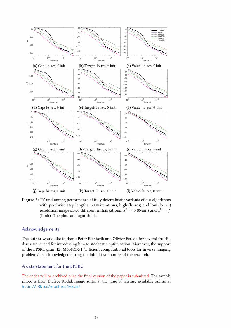
101 102 103

Iteration

-200

-150

-100

-50dB

(a) Gap: lo-res, f-init

101 102 103

Iteration

-140

-120

-100

-80

-60

-40

-20

(b) Target: lo-res, f-init

101 102 103

Iteration

-160

-140

-120

-100

-80

-60

-40

-20 PDHGMRelaxA-DRIMA-DRBMA-DDIMA-DDBM

(c) Value: lo-res, f-init

101 102 103

Iteration

-200

-150

-100

dB

(d) Gap: lo-res, 0-init

101 102 103

Iteration

-140

-120

-100

-80

-60

-40

-20

(e) Target: lo-res, 0-init

101 102 103

Iteration

-160

-140

-120

-100

-80

-60

-40

-20

(f) Value: lo-res, 0-init

101 102 103

Iteration

-140

-120

-100

-80

-60

-40

dB

(g) Gap: hi-res, f-init

101 102 103

Iteration

-100

-80

-60

-40

-20

(h) Target: hi-res, f-init

101 102 103

Iteration

-120

-100

-80

-60

-40

-20

(i) Value: hi-res, f-init

101 102 103

Iteration

-160

-140

-120

-100

-80

-60

dB

(j) Gap: hi-res, 0-init

101 102 103

Iteration

-100

-80

-60

-40

-20

(k) Target: hi-res, 0-init

101 102 103

Iteration

-120

-100

-80

-60

-40

-20

(l) Value: hi-res, 0-init

Figure 5: TV undimming performance of fully deterministic variants of our algorithmswith pixelwise step lengths, 5000 iterations, high (hi-res) and low (lo-res)resolution images.Two dierent initialisations: x0 “ 0 (0-init) and x0 “ f(f-init). The plots are logarithmic.

Acknowledgements

The author would like to thank Peter Richtárik and Olivier Fercoq for several fruitfuldiscussions, and for introducing him to stochastic optimisation. Moreover, the supportof the EPSRC grant EP/M00483X/1 “Ecient computational tools for inverse imagingproblems” is acknowledged during the initial two months of the research.

A data statement for the EPSRC

The codes will be archived once the nal version of the paper is submitted. The samplephoto is from thefree Kodak image suite, at the time of writing available online athttp://r0k.us/graphics/kodak/.

39

A. Proofs of the general estimates

Here, we prove Theorems 2.1 to 2.3. In fact, as the technique streamlines the proof, weconsider instead of (PP) for convex Vi`1 : X ˆ Y Ñ R the general iteration

0 P Zi`1Wi`1Hpui`1q ` BVi`1pu

i`1q. (B-PP)

Our motivation is that under (C0), Zi`1Li`1 is self-adjoint, which has the eect

Zi`1Li`1pui`1 ´ uiq “ ∇Vi`1pu

i`1q for Vi`1puq :“12u ´ ui2Zi`1Li`1

. (A.1)

In (B-PP), we therefore take Vi to be an arbitrary convex function satisfying for eachi P N for some ∆i`1 P LpX ˆ Y ;X ˆ Y q and δi ě 0 the condition

Vi`1puq`δi`1 ď Vipuq`xp,ui´uy`

12u´ui2ZiΞi pΓq`∆i`1pΓq

, pu P XˆY , p P BVipuiqq.

(B-C0)

Example A.1. For the choice (A.1), using (2.10) in (B-C0), we obtain the requirement

0 ď12u ´ ui´12ZiLi ` xp,u

i ´ uy ´12u ´ ui2ZiLi , pu P X ˆ Y q, (A.2)

where p “ L˚i Z˚i pu

i ´ ui´1q. We observe for self-adjoint M the identity

xui ´ ui´1,ui ´ uyM “12ui ´ ui´12M ´

12ui´1 ´ u2M `

12ui ´ u2M .

Applying this to M “ ZiLi , we verify (A.2) for δi :“ 12u

i ´ ui´12ZiLi . By (C0), δi ě 0.

Example A.2 (Bregman distances, cf. [52]). Suppose that V is a Bregman distance, thatis, for some convex function J and some pi P BJpuiq to be xed, we take

Vi`1puq “ Jpuq ´ xpi ,u ´ uiy ´ Jpuiq.

Then (B-C0) is satised ∆i`1pΓq “ ZiΞipΓq if

Jpuq ´ xpi ,u ´ui`1y ´ Jpui`1q ď Jpuq ´ xpi´1,u ´uiy ´ Jpuiq ` xp,ui`1´uy. (A.3)

We have p P BVipuiq if and only if p P BJpuiq ´ pi´1. Taking pi :“ p ` pi´1, (A.3)

becomes

xp ` pi ,ui`1 ´ uy ´ Jpui`1q ď ´xpi ,u ´ uiy ´ Jpuiq ` xp,ui`1 ´ uy.

In other wordsJpuiq ` xpi ,u

i`1 ´ uiy ď Jpui`1q.

This automatically holds by the convexity of J . Since there is no acceleration, Theo-rem A.1 will not give any kind of convergence rates for this choice of Vi . We at mostobtain obtain the convergence of the ergodic gap from Lemma A.1.

For better rates, we need more structure, and to incorporate acceleration parametersin Vi . Normally in the algorithm (2.2) & (2.3), we would for c “ K2p1´ δq have

Zi`1Li`1 “

ˆ

τ´2i I ´τ´1

i K˚

´τ´1i K cI

˙

This suggests to use

Vi`1puq “ τ´2i Vx,i`1pxq ` cVy ,i`1pyq ´ τ´1

i xKpx ´ x iq,y ´ y iy

for Vx,i`1 and Vy ,i`1 the Bregman distances corresponding to some Jx and Jy at x i andy i . If Jx and Jy possess sucient strong convexity, Vi`1 will also be strongly convex. Inthat case, we could by adapting (C1) and the analysis of Example A.2, get convergencesimilar to [52].

40

We have the following abstract convergence estimate. To keep the necessary setupshort, and to avoid introducing additional notation, we do not represent the result inthe full generality of Banach spaces. Such a generalisation is, however, immediate.

Theorem A.1. Let us be given K P LpX ;Y q, and convex, proper, lower semicontinuousfunctionals G : X Ñ R and F˚ : Y Ñ R on Hilbert spaces X and Y , satisfying (G-PM)and (F˚-PM) for some 0 ď Γ P LpX ;X q. Suppose (B-PP) is solvable, and that (B-C0) issatised for each i P N for some operators Ti ,Φi P LpX ;X q and Σi`1,Ψi`1 P LpY ;Y q,with ΦiTi P T and Ψi`1Σi`1 P S. Then the iterates ui “ px i ,y iq of (B-PP) satisfy

VN`1ppuq `N´1ÿ

i“0δi`1 ď V0ppuq `

12

N´1ÿ

i“0ui`1 ´ pu2∆i`2pΓq

, pN ě 1q (A.4)

Proof. We take pi`1 P Hpui`1q such that ´Zi`1Wi`1pi`1 P BVi`1pu

i`1q, guaranteed toexist by the iteration (B-PP) being by assumption solvable. Using the expansion

Zi`1Wi`1 “

ˆ

ΦiTi 00 Ψi`1Σi`1

˙

,

and the fact that 0 P Hppuq, we deduce

xpi`1,W˚i`1Z

˚i`1pu

i`1 ´ puqy Ă xHpui`1q ´ Hppuq,W ˚i`1Z

˚i`1pu

i`1 ´ puqy

“ xBGpx i`1q ´ BGppxq,T ˚i Φ˚i px

i`1 ´ pxqy

` xBF˚py i`1q ´ BF˚ppyq,Σ˚i`1Ψ˚i`1py

i`1 ´ pyqy

` xK˚py i`1 ´ pyq,T ˚i Φ˚i px

i`1 ´ pxqy

´ xKpx i`1 ´ pxq,Σ˚i`1Ψ˚i`1py

i`1 ´ pyqy.

An application of (G-PM) and (F˚-PM) consequently gives

xpi`1,W˚i`1Z

˚i`1pu

i`1 ´ puqy ě x i`1 ´ px2ΦiTi Γ

` xΦiTiK˚py i`1 ´ pyq,x i`1 ´ pxy

´ xΨi`1Σi`1Kpxi`1 ´ pxq,y i`1 ´ pyy.

“12ui`1 ´ pu2Zi`1Ξi`1pΓq

.

(A.5)

Next, (B-C0) at u “ pu gives

Vi`1ppuq´Vi`2ppuq´δi`1`12ui`1´pu2Zi`1Ξi`1pΓq`∆i`2pΓq

ě xZi`1Wi`1pi`1,ui`1´puy.

(A.6)Combining (A.5) with (A.6), we thus deduce

Vi`2ppuq ` δi`1 ď Vi`1ppuq `12ui`1 ´ pu2∆i`2pΓq

. (A.7)

Summing (A.7) over i “ 0, . . . ,N ´ 1, we obtain (A.4).

Proof of Theorem 2.1. Insert Vi from (A.1) into (A.4), and use Theorem A.1 and Exam-ple A.1.

Lemma A.1. LetX andY be Hilbert spaces,K P LpX ;Y q, andG : X Ñ R and F˚ : Y Ñ R

be convex, proper, lower semicontinuous. Take 0 ď Γ P LpX ;X q. Suppose (B-PP) issolvable, and that (B-C0) is satised for each i P N for some Ti ,Φi P LpX ;X q and

41

Σi`1,Ψi`1 P LpY ;Y q, with ΦiTi P T and Ψi`1Σi`1 P S. Then the iterates ui “ px i ,y iqof (B-PP) satisfy

VN`1ppuq `N´1ÿ

i“0

`

G1i`1 ` δi`1˘

ď V0ppuq `12

N´1ÿ

i“0ui`1 ´ pu2∆i`2pΓ2q, pN ě 1q (A.8)

for

G1i`1 :“xBGpx i`1q,T ˚i Φ˚i px

i`1 ´ pxqy ´ x i`1 ´ px2ΦiTi Γ2

` xBF˚py i`1q,Σ˚i`1Ψ˚i`1py

i`1 ´ pyqy

´ xpy ,pKT ˚i Φ˚i ´ Ψi`1Σi`1Kqpxy ´ xy

i`1,Ψi`1Σi`1Kpxy ` xpy ,KT˚i Φ

˚i x

i`1y.

Proof. Similarly to the proof of Theorem 2.1, we takepi`i P Hpui`1q such that´Zi`1pi`i PBVi`1pu

i`1q, guaranteed to exist by the iteration (B-PP) being by assumption solvable.Then

xZi`1Wi`1pi`i ,ui`1 ´ puy “ xBGpx i`1q,T ˚i Φ

˚i px

i`1 ´ pxqy

` xBF˚py i`1q,Σ˚i`1Ψ˚i`1py

i`1 ´ pyqy

` xK˚y i`1,T ˚i Φ˚i px

i`1 ´ pxqy ´ xKx i`1,Σ˚i`1Ψ˚i`1py

i`1 ´ pyqy

“ дi`1 ` xi`1 ´ px2ΦiTi Γ2

` xy i`1,pKT ˚i Φ˚i ´ Ψi`1Σi`1Kqx

i`1y

´ xy i`1,KT ˚i Φ˚i pxy ` xpy ,Ψi`1Σi`1Kx

i`1y.

for

дi`1 :“ xBGpx i`1q,T ˚i Φ˚i px

i`1´pxqy´x i`1´px2ΦiTi Γ2`xBF˚py i`1q,Σ˚i`1Ψ

˚i`1py

i`1´pyqy.

A little bit of reorganisation and referral to the expression for ∆i`1 in (2.9) gives

xZi`1Wi`1pi`i ,ui`1 ´ puy ě дi`1 ` x

i`1 ´ px2ΦiTi Γ2

` xy i`1 ´ py ,pKT ˚i Φ˚i ´ Ψi`1Σi`1Kqpx

i`1 ´ pxqy

´ xpy ,pKT ˚i Φ˚i ´ Ψi`1Σi`1Kqpxy

´ xy i`1,Ψi`1Σi`1Kpxy ` xpy ,KT˚i Φ

˚i x

i`1y

“ G1i`1 `12ui`1 ´ pu2Ξi`1pΓ2q.

Combining (A.6) and (A.9), we obtain

Vi`2ppuq ` G1i`1 ` δi`1 ď Vi`1ppuq `

12ui`1 ´ pu2∆i`2pΓ2q.

Summing this for i “ 0, . . . ,N ´ 1 gives (A.8).

Proof of Theorem 2.2. We use Lemma A.1. We already veried (B-C0) in Example A.1,so it remains to derive (2.17). Using (CG), (G-EC), and (F˚-EC), we compute

N´1ÿ

i“0ErG1i`1s :“

N´1ÿ

i“0E”

xBGpx i`1q,T ˚i Φ˚i px

i`1 ´ pxqy ´ x i`1 ´ px2ΦiTi Γ2

ı

` E“

xBF˚py i`1q,Σ˚i`1Ψ˚i`1py

i`1 ´ pyqy‰

´ ζN xryN ,Kpxy ` ζN xpy ,KrxN y

ě ζNGprxN ,ryN q ´ ζN xryN ,Kpxy ` ζN xpy ,KrxN y.

We therefore obtain (2.17) by taking the expectation in (A.8).

42

Proof of Theorem 2.3. Using (G-PM) and (OC), we deduce

G11 ě xBF˚py1q,Σ˚1Ψ

˚1 py

1 ´ pyqy ` xpy ,Ψ1Σ1Kpxy ´ xy1,Ψ1Σ1Kpxy.

Likewise (F˚-PM) and (OC) give

G1N ě xBGpxN q,T ˚N´1Φ

˚N´1px

N ´ pxqy ´ xN ´ px2ΦN´1TN´1Γ2

´ xpy ,KT ˚N´1Φ˚N´1pxy ` xpy ,KT

˚N´1Φ

˚N´1x

N y.

Shifting indices of y i by one compared to G1i`1, we dene

G1 ,i`1 :“xBGpx i`1q,T ˚i Φ˚i px

i`1 ´ pxqy ´ x i`1 ´ px2ΦiTi Γ2

` xBF˚py iq,Σ˚i Ψ˚i py

i ´ pyqy

´ xpy ,pKT ˚i Φ˚i ´ ΨiΣiKqpxy ´ xy

i ,ΨiΣiKpxy ` xpy ,KT˚i Φ

˚i x

i`1y,

Correspondingly reorganising terms, we observe

N´1ÿ

i“0G1i`1 “ G

11 `

N´2ÿ

i“1G1i`1 ` G

1N ě

N´1ÿ

i“1G1 ,i`1.

We now estimateřN´1

i“1 ErG1 ,i`1s analogously to the proof of Theorem 2.2.

B. An inequality

We needed the following for convergence rates in Section 4.2.

Lemma B.1. Suppose ϕN ě ϕ0 ` břN´1

i“0 pi ` 1qp for each N ě 0 for some constantsp ě 0 and ϕ0,b ą 0. Then ϕN ě ϕ0 `CN p`1 for some constant C “ Cpb,ϕ0,pq ą 0.

Proof. We calculate

ϕN ě ϕ0 ` bNÿ

i“1ip ě ϕ0 ` b

ż N

2xp dx ě ϕ0 ` p´1bpN p`1 ´ 2q.

The lower bound ϕN ě ϕ0 for 0 ď N ď 2, and suitably choice of C ą 0 verify theclaim.

References

[1] J. Bolte, S. Sabach and M. Teboulle, Proximal alternating linearized minimizationfor nonconvex and nonsmooth problems, Mathematical Programming 146 (2013),459–494, doi:10.1007/s10107-013-0701-9.

[2] T. Möllenho, E. Strekalovskiy, M. Moeller and D. Cremers, The primal-dual hybridgradient method for semiconvex splittings, SIAM Journal on Imaging Sciences 8(2015), 827–857, doi:10.1137/140976601.

[3] T. Valkonen and T. Pock, Acceleration of the PDHGM on partially strongly convexfunctions (2015), submitted, arXiv:1511.06566.URL http://iki.fi/tuomov/mathematics/cpaccel.pdf

[4] P. Ochs, Y. Chen, T. Brox and T. Pock, iPiano: Inertial proximal algorithm fornon-convex optimization (2014), preprint, arXiv:1404.4805.

43

[5] L. Rudin, S. Osher and E. Fatemi, Nonlinear total variation based noise removalalgorithms, Physica D 60 (1992), 259–268.

[6] K. Bredies, K. Kunisch and T. Pock, Total generalized variation, SIAM Journal onImaging Sciences 3 (2011), 492–526, doi:10.1137/090769521.

[7] A. Chambolle and P.-L. Lions, Image recovery via total variation mini-mization and related problems, Numerische Mathematik 76 (1997), 167–188,doi:10.1007/s002110050258.

[8] I. Daubechies, M. Defrise and C. De Mol, An iterative thresholding algorithm forlinear inverse problems with a sparsity constraint, Communications on Pure andApplied Mathematics 57 (2004), 1413–1457, doi:10.1002/cpa.20042.

[9] I. Loris and C. Verhoeven, On a generalization of the iterative soft-thresholdingalgorithm for the case of non-separable penalty, Inverse Problems 27 (2011), 125007,doi:10.1088/0266-5611/27/12/125007.

[10] A. Beck and M. Teboulle, A fast iterative shrinkage-thresholding algorithm forlinear inverse problems, SIAM Journal on Imaging Sciences 2 (2009), 183–202,doi:10.1137/080716542.

[11] S. Wright, Coordinate descent algorithms, Mathematical Programming 151 (2015),3–34, doi:10.1007/s10107-015-0892-3.

[12] Y. Nesterov, Eciency of coordinate descent methods on huge-scale optimizationproblems, SIAM Journal on Optimization 22 (2012), 341–362, doi:10.1137/100802001.

[13] P. Richtárik and M. Takáč, Parallel coordinate descent methods for big data optimiza-tion, Mathematical Programming (2015), 1–52, doi:10.1007/s10107-015-0901-6.

[14] O. Fercoq and P. Richtárik, Accelerated, parallel and proximal coordinate descent(2013), preprint, arXiv:1312.5799.

[15] P. Richtárik and M. Takáč, Distributed coordinate descent method for learning withbig data (2013), arXiv:1310.2059.

[16] Z. Qu, P. Richtárik and T. Zhang, Randomized dual coordinate ascent with arbitrarysampling (2014), preprint, arXiv:1411.5873.

[17] P. Zhao and T. Zhang, Stochastic optimization with importance sampling (2014),preprint, arXiv:1401.2753.

[18] S. Shalev-Shwartz and T. Zhang, Accelerated proximal stochastic dual coordinateascent for regularized loss minimization, Mathematical Programming 155 (2014),105–145, doi:10.1007/s10107-014-0839-0.

[19] Z. Qu, P. Richtárik, M. Takáč and O. Fercoq, SDNA: stochastic dual newton ascentfor empirical risk minimization (2015), arXiv:1502.02268.

[20] D. Csiba, Z. Qu and P. Richtárik, Stochastic dual coordinate ascent with adaptiveprobabilities, preprint, arXiv:1502.08053.

[21] P. L. Combettes and J.-C. Pesquet, Stochastic forward-backward and primal-dualapproximation algorithms with application to online image restoration (2016),arXiv:1602.08021.

44

[22] Z. Peng, Y. Xu, M. Yan and W. Yin, ARock: an algorithmic framework for asyn-chronous parallel coordinate updates (2015), uCLA CAM Report 15-37.URL ftp://ftp.math.ucla.edu/pub/camreport/cam15-37.pdf

[23] A. Chambolle and T. Pock, A rst-order primal-dual algorithm for convex problemswith applications to imaging, Journal of Mathematical Imaging and Vision 40 (2011),120–145, doi:10.1007/s10851-010-0251-1.

[24] T. Pock, D. Cremers, H. Bischof and A. Chambolle, An algorithm for minimizingthe mumford-shah functional, in: 12th IEEE Conference on Computer Vision, 2009,1133–1140, doi:10.1109/ICCV.2009.5459348.

[25] E. Esser, X. Zhang and T. F. Chan, A general framework for a class of rst orderprimal-dual algorithms for convex optimization in imaging science, SIAM Journalon Imaging Sciences 3 (2010), 1015–1046, doi:10.1137/09076934X.

[26] D. Gabay, Applications of the method of multipliers to variational inequalities,in: Augmented Lagrangian Methods: Applications to the Numerical Solution ofBoundary-Value Problems, volume 15, Edited by M. Fortin and R. Glowinski, North-Holland1983, 299–331.

[27] J. Douglas, Jim and J. Rachford, H. H., On the numerical solution of heat conductionproblems in two and three space variables, Transactions of the American Mathemat-ical Society 82 (1956), pp. 421–439, doi:10.2307/1993056.

[28] K. Bredies and H. P. Sun, Preconditioned Douglas–Rachford algorithms for TV- andTGV-regularized variational imaging problems, Journal of Mathematical Imagingand Vision 52 (2015), 317–344, doi:10.1007/s10851-015-0564-1.

[29] T. Goldstein and S. Osher, The split bregman method for l1-regularized problems,SIAM Journal on Imaging Sciences 2 (2009), 323–343, doi:10.1137/080725891.

[30] W. Yin, S. Osher, D. Goldfarb and J. Darbon, Bregman iterative algorithms for `1-minimization with applications to compressed sensing, SIAM Journal on ImagingSciences 1 (2008), 143–168, doi:10.1137/070703983.

[31] S. Setzer, Operator splittings, Bregman methods and frame shrinkage in im-age processing, International Journal of Computer Vision 92 (2011), 265–280,doi:10.1007/s11263-010-0357-3.

[32] T. Suzuki, Stochastic dual coordinate ascent with alternating direction multipliermethod (2013), preprint, arXiv:1311.0622.

[33] Y. Zhang and L. Xiao, Stochastic primal-dual coordinate method for regularizedempirical risk minimization (2014), arXiv:1409.3257.

[34] O. Fercoq and P. Bianchi, A coordinate descent primal-dual algorithm with largestep size and possibly non separable functions (2015), arXiv:1508.04625.

[35] P. Bianchi, W. Hachem and F. Iutzeler, A stochastic coordinate descent primal-dual algorithm and applications to large-scale composite optimization, preprint,arXiv:1407.0898.

[36] Z. Peng, T. Wu, Y. Xu, M. Yan and W. Yin, Coordinate friendly structures, algorithmsand applications (2016), arXiv:1601.00863.

45

[37] J.-C. Pesquet and A. Repetti, A class of randomized primal-dual algorithms fordistributed optimization (2014), arXiv:1406.6404.

[38] A. W. Yu, Q. Lin and T. Yang, Doubly stochastic primal-dual coordinate method for em-pirical risk minimization and bilinear saddle-point problem (2015), arXiv:1508.03390.

[39] C. Chen, B. He, Y. Ye and X. Yuan, The direct extension of ADMM for multi-blockconvex minimization problems is not necessarily convergent, Mathematical Program-ming 155 (2014), 57–79, doi:10.1007/s10107-014-0826-5.

[40] A. S. Lewis and S. Zhang, Partial smoothness, tilt stability, and generalized hessians,SIAM Journal on Optimization 23 (2013), 74–94, doi:10.1137/110852103.

[41] A. S. Lewis, Active sets, nonsmoothness, and sensitivity, SIAM Journal on Optimiza-tion 13 (2002), 702–725, doi:10.1137/S1052623401387623.

[42] J. Liang, J. Fadili and G. Peyré, Local linear convergence of forward–backward underpartial smoothness, Advances in Neural Information Processing Systems 27 (2014),1970–1978.URL http://papers.nips.cc/paper/5260-local-linear-convergence-of-

forward-backward-under-partial-smoothness.pdf

[43] T. Pock and A. Chambolle, Diagonal preconditioning for rst order primal-dual algo-rithms in convex optimization, in: Computer Vision (ICCV), 2011 IEEE InternationalConference on, 2011, 1762 –1769, doi:10.1109/ICCV.2011.6126441.

[44] B. He and X. Yuan, Convergence analysis of primal-dual algorithms for a saddle-pointproblem: From contraction perspective, SIAM Journal on Imaging Sciences 5 (2012),119–149, doi:10.1137/100814494.

[45] A. N. Shiriaev, Probability, Graduate Texts in Mathematics, Springer1996.

[46] A. Chambolle and T. Pock, On the ergodic convergence rates of a rst-order primal–dual algorithm, Mathematical Programming (2015), 1–35, doi:10.1007/s10107-015-0957-3.

[47] Y. Chen, G. Lan and Y. Ouyang, Optimal primal-dual methods for a class ofsaddle point problems, SIAM Journal on Optimization 24 (2014), 1779–1814,doi:10.1137/130919362.

[48] T. Goldstein, M. Li and X. Yuan, Adaptive primal-dual splitting methods for statisticallearning and image processing, Advances in Neural Information Processing Systems28 (2015), 2080–2088.

[49] T. Valkonen, K. Bredies and F. Knoll, Total generalised variation in diu-sion tensor imaging, SIAM Journal on Imaging Sciences 6 (2013), 487–525,doi:10.1137/120867172.URL http://iki.fi/tuomov/mathematics/dtireg.pdf

[50] J. C. de Los Reyes, C.-B. Schönlieb and T. Valkonen, Bilevel parameter learn-ing for higher-order total variation regularisation models, Journal of Mathemat-ical Imaging and Vision (2016), doi:10.1007/s10851-016-0662-8, published online,arXiv:1508.07243.URL http://iki.fi/tuomov/mathematics/tgv_learn.pdf

[51] A. Chambolle, An algorithm for mean curvature motion, Interfaces and Free Bound-aries 6 (2004), 195.

46

[52] T. Hohage and C. Homann, A generalization of the Chambolle-Pock algorithm toBanach spaces with applications to inverse problems (2014), preprint, arXiv:1412.0126.

47