Blocken

ARTICLE IN PRESS

1352-2310/$ - se

doi:10.1016/j.at

�Correspondfax: +3140 243

E-mail addr

Atmospheric Environment 41 (2007) 238–252

www.elsevier.com/locate/atmosenv

CFD simulation of the atmospheric boundary layer:wall function problems

Bert Blockena,�, Ted Stathopoulosb, Jan Carmelieta,c

aBuilding Physics and Systems, Technische Universiteit Eindhoven, P.O. Box 513, 5600 MB Eindhoven, The NetherlandsbDepartment of Building, Civil and Environmental Engineering, Concordia University, 1455 de Maisonneuve Blvd West,

Montreal, Que., Canada, H3G 1M8cLaboratory of Building Physics, Department of Civil Engineering, Katholieke Universiteit Leuven, Kasteelpark Arenberg 40,

3001 Leuven, Belgium

Received 17 May 2006; received in revised form 14 August 2006; accepted 15 August 2006

Abstract

Accurate Computational Fluid Dynamics (CFD) simulations of atmospheric boundary layer (ABL) flow are essential

for a wide variety of atmospheric studies including pollutant dispersion and deposition. The accuracy of such simulations

can be seriously compromised when wall-function roughness modifications based on experimental data for sand-grain

roughened pipes and channels are applied at the bottom of the computational domain. This type of roughness modification

is currently present in many CFD codes including Fluent 6.2 and Ansys CFX 10.0, previously called CFX-5. The problems

typically manifest themselves as unintended streamwise gradients in the vertical mean wind speed and turbulence profiles

as they travel through the computational domain. These gradients can be held responsible—at least partly—for the

discrepancies that are sometimes found between seemingly identical CFD simulations performed with different CFD codes

and between CFD simulations and measurements. This paper discusses the problem by focusing on the simulation of a

neutrally stratified, fully developed, horizontally homogeneous ABL over uniformly rough, flat terrain. The problem and

its negative consequences are discussed and suggestions to improve the CFD simulations are made.

r 2006 Elsevier Ltd. All rights reserved.

Keywords: Computational Fluid Dynamics (CFD); Numerical simulation; Atmospheric boundary layer (ABL); Sustainable boundary

layer; Equilibrium vertical profiles; Horizontal homogeneity

1. Introduction

Computational Fluid Dynamics (CFD) is increas-ingly being used to study a wide variety of processesin the lower parts of the atmospheric boundarylayer (ABL) (0–200m) including pollutant disper-

e front matter r 2006 Elsevier Ltd. All rights reserved

mosenv.2006.08.019

ing author. Tel.: +31 40 247 2138;

8595.

ess: [email protected] (B. Blocken).

sion and deposition, wind-driven rain, buildingventilation, etc. Recently, comprehensive literaturereviews on the use of CFD for these applicationshave been published (Stathopoulos, 1997; Reichrathand Davies, 2002; Blocken and Carmeliet, 2004;Bitsuamlak et al., 2004; Meroney, 2004; Frankeet al., 2004).

Accurate simulation of ABL flow in the compu-tational domain is imperative to obtain accurateand reliable predictions of the related atmospheric

.

www.elsevier.com/locate/atmosenv

dx.doi.org/10.1016/j.atmosenv.2006.08.019

mailto:[email protected]

ARTICLE IN PRESS

Nomenclature

B integration constant in the log lawCS roughness constantCe1, Ce2, Cm constants in the k–e modele inhomogeneity error, %E empirical constant for a smooth wall in

wall function (E9.793)k turbulent kinetic energy, m2 s�2

kS equivalent sand-grain roughness height,m

kS+ dimensionless equivalent sand-grain

roughness heightL, H length and height of computational

domain, mP centre point of wall-adjacent cellTI turbulence intensityut wall-function friction velocity, m s�1

u� wall-function friction velocity, m s�1

u�ABL ABL friction velocity, m s�1

u+ dimensionless mean streamwise windspeed

U mean streamwise wind speed, m s�1

x, y streamwise and height co-ordinates, my0 aerodynamic roughness length, myP distance from point P to the wall, my+ dimensionless wall unite turbulence dissipation rate, m2 s�3

k von Karman constant (0.40–0.42)m dynamic molecular viscosity, kgm�1 s�1

mt dynamic turbulent viscosity, kgm�1 s�1

n kinematic molecular viscosity, m2 s�1

r fluid density, kgm�3

se constant in the k–e modeltw wall shear stress, Paj flow variableo specific dissipation rate, s�1

DB roughness functionDx control volume length, m

B. Blocken et al. / Atmospheric Environment 41 (2007) 238–252 239

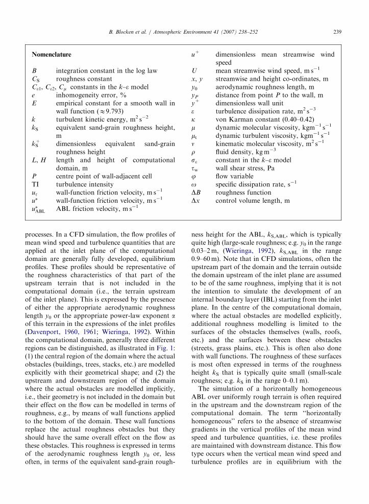
processes. In a CFD simulation, the flow profiles ofmean wind speed and turbulence quantities that areapplied at the inlet plane of the computationaldomain are generally fully developed, equilibriumprofiles. These profiles should be representative ofthe roughness characteristics of that part of theupstream terrain that is not included in thecomputational domain (i.e., the terrain upstreamof the inlet plane). This is expressed by the presenceof either the appropriate aerodynamic roughnesslength y0 or the appropriate power-law exponent aof this terrain in the expressions of the inlet profiles(Davenport, 1960, 1961; Wieringa, 1992). Withinthe computational domain, generally three differentregions can be distinguished, as illustrated in Fig. 1:(1) the central region of the domain where the actualobstacles (buildings, trees, stacks, etc.) are modelledexplicitly with their geometrical shape; and (2) theupstream and downstream region of the domainwhere the actual obstacles are modelled implicitly,i.e., their geometry is not included in the domain buttheir effect on the flow can be modelled in terms ofroughness, e.g., by means of wall functions appliedto the bottom of the domain. These wall functionsreplace the actual roughness obstacles but theyshould have the same overall effect on the flow asthese obstacles. This roughness is expressed in termsof the aerodynamic roughness length y0 or, lessoften, in terms of the equivalent sand-grain rough-

ness height for the ABL, kS,ABL, which is typicallyquite high (large-scale roughness; e.g. y0 in the range0.03–2m, (Wieringa, 1992), kS,ABL in the range0.9–60m). Note that in CFD simulations, often theupstream part of the domain and the terrain outsidethe domain upstream of the inlet plane are assumedto be of the same roughness, implying that it is notthe intention to simulate the development of aninternal boundary layer (IBL) starting from the inletplane. In the centre of the computational domain,where the actual obstacles are modelled explicitly,additional roughness modelling is limited to thesurfaces of the obstacles themselves (walls, roofs,etc.) and the surfaces between these obstacles(streets, grass plains, etc.). This is often also donewith wall functions. The roughness of these surfacesis most often expressed in terms of the roughnessheight kS that is typically quite small (small-scaleroughness; e.g. kS in the range 0–0.1m).

The simulation of a horizontally homogeneousABL over uniformly rough terrain is often requiredin the upstream and the downstream region of thecomputational domain. The term ‘‘horizontallyhomogeneous’’ refers to the absence of streamwisegradients in the vertical profiles of the mean windspeed and turbulence quantities, i.e. these profilesare maintained with downstream distance. This flowtype occurs when the vertical mean wind speed andturbulence profiles are in equilibrium with the

ARTICLE IN PRESS

downstream part ofcomputationaldomain

central part of computationaldomain

incident flow

approach flow

inlet flow

inlet plane

upstream part of computationaldomain

outlet plane

Fig. 1. Computational domain with building models for CFD simulation of ABL flow—definition of inlet flow, approach flow and

incident flow and indication of different parts in the domain for roughness modelling.

B. Blocken et al. / Atmospheric Environment 41 (2007) 238–252240

roughness characteristics of the ground surface.Concerning the upstream part of the domain, adistinction is made between inlet flow, approachflow and incident flow (Fig. 1). The ‘‘approachflow’’ profiles are those travelling towards thebuilding models, while the ‘‘incident flow’’ profilesare those obtained in a similar but empty computa-tional domain, at the position where the buildingswould be positioned. Horizontal homogeneity im-plies that the inlet profiles, the approach flowprofiles and the incident profiles are the same.

In the past, several authors have reporteddifficulties in simulating a horizontally homoge-neous ABL flow in at least the upstream part ofcomputational domains. Richards and Younis(1990), discussing the work of Mathews (1987),referred to a situation in which the approach flowchanged rapidly in the upstream region of thecomputational domain. A particular observationwas the considerable acceleration of the flow nearthe surface. Zhang (1994), using the k–e model andthe standard wall functions (Launder and Spalding,1974) without roughness modification, reported anunwanted change in the profiles of mean wind speedand especially turbulent kinetic energy, which hesuggested to be responsible for some of thediscrepancies found between the CFD simulationsand the corresponding wind tunnel measurements.A similar problem for turbulent kinetic energy wasreported by Quinn et al. (2001) who used the k–emodel in CFX-4.1. Riddle et al. (2004), employingFluent 6 with the k–e and the Reynolds stress model(RSM), observed significant profile changes in an

empty computational domain, especially for theturbulent kinetic energy. Problems in simulating ahorizontally homogeneous ABL flow were alsoreported by Miles and Westbury (2003), usingCFX-5, and by Franke et al. (2004), Franke andFrank (2005) and Blocken and Carmeliet (2006)using Fluent 5 and 6.

The unintended differences between inlet profilesand incident profiles (i.e. the horizontal homogene-ity problem) can be detrimental for the success ofCFD simulations given that even minor changes tothe incident flow profiles can cause significantchanges in the flow field. Indeed, sensitivity studiesby Castro and Robins (1977), Miles and Westbury(2003), Gao and Chow (2005) and Blocken et al.(2006) have indicated the important influence of theshape of the vertical incident flow profiles on thesimulation results of flow around buildings.Furthermore, the considerable problems in simulat-ing the simple case of a horizontally homogeneousABL flow suggest that similar or maybe even moreserious problems can be expected when morecomplex cases of ABL flow have to be simulated,e.g. the development of IBLs over terrains withroughness changes.

This paper addresses the problem of horizontalhomogeneity associated with the use of sand-grainroughness wall functions. This is done by focusingon the CFD simulation of a neutrally stratified,horizontally homogeneous ABL flow over uni-formly rough, flat terrain. The reasons for thedifficulties possibly encountered are explained, thenegative consequences involved are discussed and

ARTICLE IN PRESSB. Blocken et al. / Atmospheric Environment 41 (2007) 238–252 241

suggestions to handle them are made. First, inSection 2, the basic requirements for a CFDsimulation of ABL flow with sand-grain wallfunctions are set. Section 3 describes the commonlyused, fully developed ABL inlet profiles for meanwind speed, turbulent kinetic energy and turbulencedissipation rate. In Section 4, the so-called sand-grain roughness wall-function modification is brieflydescribed. Section 5 points to the inconsistency ofthe basic requirements for ABL flow simulationwith these wall functions. In Section 6, the typicalnegative consequences of this inconsistency arediscussed. Section 7 summarizes various remedialmeasures. Finally, Section 8 concludes the paper.

2. Basic requirements for ABL flow simulation

In almost all CFD simulations of the lower partof the ABL, an accurate description of the flow nearthe ground surface is required. In such cases, if thewall roughness is expressed by an equivalent sand-grain roughness kS in the wall functions, fourrequirements should be simultaneously satisfied.This set of requirements has been distilled fromvarious sources including CFD literature and CFDsoftware manuals (Richards and Hoxey, 1993;Franke et al., 2004; Fluent Inc., 2005; Ansys Ltd.,2005):

(1)
A sufficiently high mesh resolution in thevertical direction close to the bottom of thecomputational domain (e.g. height of first cello1m);
(2)
A horizontally homogeneous ABL flow in theupstream and downstream region of the do-main;
(3)
A distance yP from the centre point P of thewall-adjacent cell to the wall (bottom ofdomain) that is larger than the physical rough-ness height kS of the terrain (yP4kS); and
(4)
Knowing the relationship between the equiva-lent sand-grain roughness height kS and thecorresponding aerodynamic roughness lengthy0.
The first requirement is important for all compu-tational studies of flow near the surface of theEarth. For instance, for pedestrian wind comfortstudies, Franke et al. (2004) state that at least 2 or 3control volume layers should be provided belowpedestrian height (1.75m). The second requirementimplies the insertion of (empirical) information

about the ground roughness (roughness of thebottom of the computational domain) into thesimulation to prevent streamwise gradients inthe flow in the upstream and downstream part ofthe domain, i.e. outside the main disturbance of theflow field by the explicitly modelled obstacles(Richards and Hoxey, 1993). This generally requiresthe use of wall functions. The third requirementimplies that it is not physically meaningful to havegrid cells with centre points within the physicalroughness height. This requirement is explicitlymentioned by several commercial CFD codesincluding Fluent 6.2 (Fluent Inc., 2005) and AnsysCFX 10.0 (Ansys Ltd., 2005). Both codes warn theuser to abide by the requirement yP4kS. Inaddition, Ansys Ltd. (2005) mentions that violationof this requirement can lead to inaccuracies and tosolver failure but it does not elaborate further onthis issue. The fourth requirement concerns arelationship that results from matching the ABLmean velocity profile and the wall function in theCFD code and will be discussed later.

All four requirements should be satisfied in theupstream and downstream region of the computa-tional domain, while in the central part, onlyrequirements (1) and (3) must be adhered to.However, it is generally impossible to satisfy allfour requirements. This paper focuses on thestandard k–e model by Jones and Launder (1972)used in combination with the standard wall func-tions by Launder and Spalding (1974). Notehowever that the validity of the findings and thestatements made in the paper is not limited to thistype of turbulence model and these wall functions.

3. Fully developed ABL profiles

For the k–e model, Richards (1989) proposedvertical profiles for the mean wind speed U,turbulent kinetic energy k and turbulence dissipa-tion rate e in the ABL that are based on the Harrisand Deaves (1981) model. Because the height of thecomputational domain is often significantly lowerthan the ABL height, these profiles are generallysimplified by assuming a constant shear stress withheight (Richards and Hoxey, 1993):

UðyÞ ¼u�ABL

kln

yþ y0

y0

� �, (1)

kðyÞ ¼u�2ABLffiffiffiffiffiffi

Cmp , (2)

ARTICLE IN PRESSB. Blocken et al. / Atmospheric Environment 41 (2007) 238–252242

�ðyÞ ¼u�3ABL

kðyþ y0Þ, (3)

where y is the height co-ordinate, u�ABL the ABLfriction velocity, k the von Karman constant(E0.40–0.42) and Cm a model constant of thestandard k–e model. It can be easily shown thatEqs. (1)–(3) are an analytical solution to thestandard k–e model if the model constants Ce1,Ce2, se, Cm are chosen in such a way that Eq. (4) issatisfied (Richards and Hoxey, 1993):

k2 ¼ ðC�2 � C�1Þs�ffiffiffiffiffiffiCm

p. (4)

Similarly, it can be shown that the set of Eqs. (2)and (5)–(6) are also an analytical solution to thesame model under the same condition (Durbin andPetterson Reif, 2001):

UðyÞ ¼u�ABL

kln

y

y0

� �, (5)

�ðyÞ ¼u�3ABL

ky. (6)

These profiles are commonly used as inlet profilesfor CFD simulations when measured profiles of U

and k are not available. It should be noted thatthese profiles are not only used for simulations withthe standard k–e model but also with other types ofturbulence models: RNG k–e, realizable k–e, stan-dard k–o, SST k–o, the Spalart–Allmaras model,

0

5

10

15

20

25

30

1 10 100y+

u+

u+ = y+κ l

ny+ + B

1

u+ =

Transitional re

g

Fullyroug

linear sublayer

buffer layer

logarithmiclayer

y+ =30y+ =5

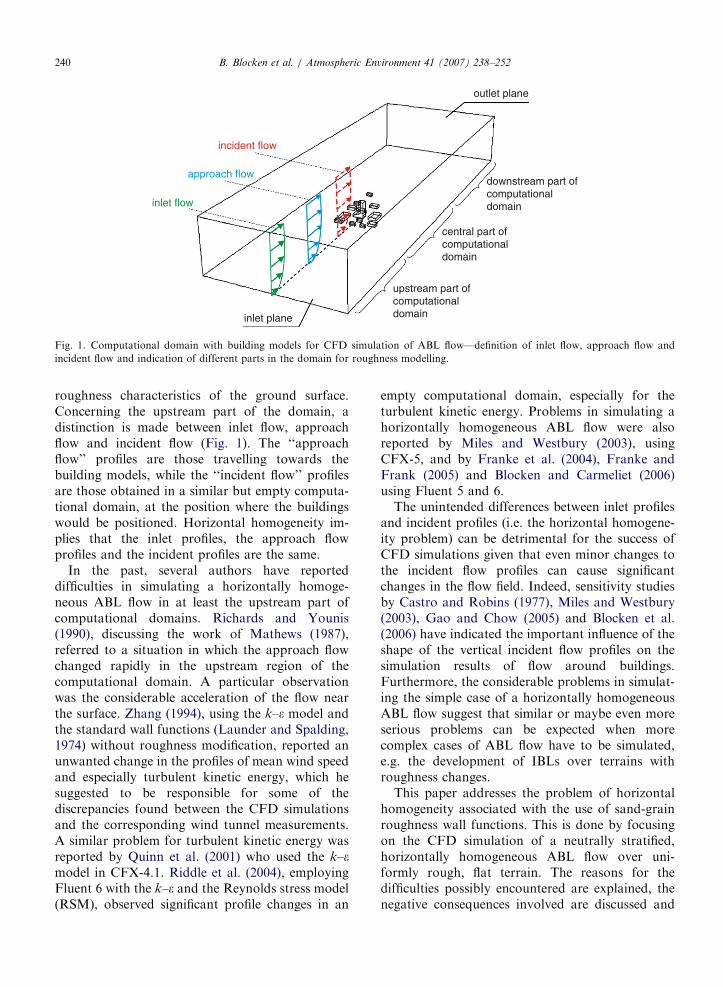
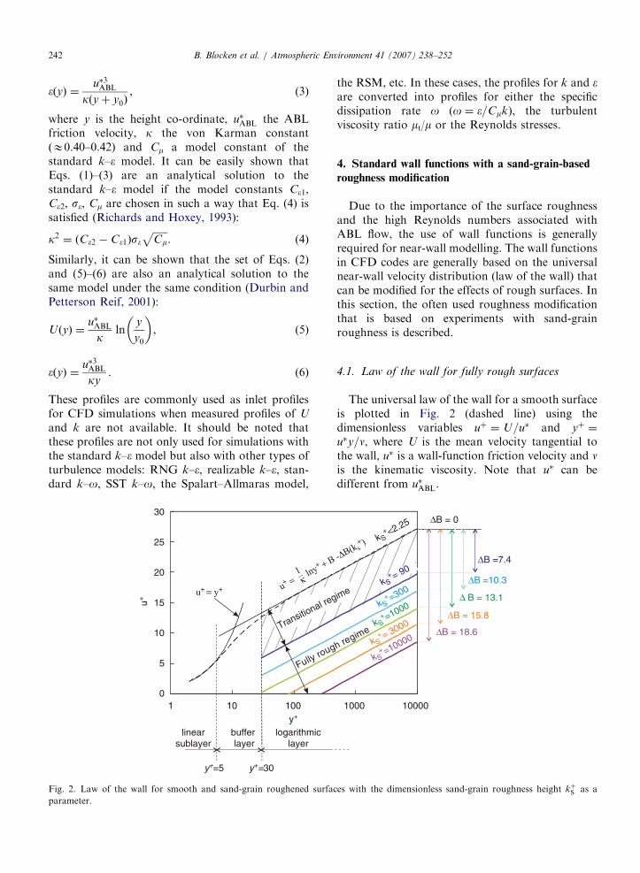
Fig. 2. Law of the wall for smooth and sand-grain roughened surfa

parameter.

the RSM, etc. In these cases, the profiles for k and eare converted into profiles for either the specificdissipation rate o (o ¼ �=Cmk), the turbulentviscosity ratio mt/m or the Reynolds stresses.

4. Standard wall functions with a sand-grain-based

roughness modification

Due to the importance of the surface roughnessand the high Reynolds numbers associated withABL flow, the use of wall functions is generallyrequired for near-wall modelling. The wall functionsin CFD codes are generally based on the universalnear-wall velocity distribution (law of the wall) thatcan be modified for the effects of rough surfaces. Inthis section, the often used roughness modificationthat is based on experiments with sand-grainroughness is described.

4.1. Law of the wall for fully rough surfaces

The universal law of the wall for a smooth surfaceis plotted in Fig. 2 (dashed line) using thedimensionless variables uþ ¼ U=u� and yþ ¼

u�y=n, where U is the mean velocity tangential tothe wall, u� is a wall-function friction velocity and nis the kinematic viscosity. Note that u� can bedifferent from u�ABL.

1000 10000

-ΔB(k s+ ) kS

+ <2.25

kS+ = 90

imekS

+ =300

kS+ =1000

kS+ = 3000

kS+ =10000

ΔB =10.3

ΔB =7.4

h regime ΔB = 18.6

ΔB = 15.8

Δ B = 13.1

ΔB = 0

ces with the dimensionless sand-grain roughness height kþS as a


The near-wall region consists of three main parts:the laminar layer or linear sublayer, the buffer layerand the logarithmic layer. In the linear sublayer, thelaminar law holds (u+ ¼ y+) while in the log layer,the logarithmic law is valid: (u+ ¼ ln(y+)/k+B)where the integration constant BE5.0–5.4 (e.g.Schlichting, 1968; White, 1991). The laminar lawis valid below about y+ ¼ 5 and the logarithmic lawabove about y+ ¼ 30 up to y+ ¼ 500–1000. Themodification of the log law for rough surfaces ismainly based on the extensive experiments byNikuradse (1933) for flow in rough, circular pipesthat were covered on the inside as tightly as possiblewith sand grains (sand-grain roughness kS). Theexperiments indicated that the mean velocitydistribution near rough walls, when plotted in asemi-logarithmic scale, as in Fig. 2, has the sameslope (1/k) but a different intercept. The shift of theintercept, DB, as shown in Fig. 2, is a function of thedimensionless sand-grain roughness height kþS ¼

u�kS=n; also called ‘‘dimensionless physical rough-ness height’’ or ‘‘roughness Reynolds number’’. Thelogarithmic law for a rough wall is (Cebeci andBradshaw, 1977):

U

u�¼

1

kln

u�y

n

� �þ B� DBðkþs Þ. (7)

The roughness function DB takes different formsdepending on the kþS value. Three regimes aredistinguished: aerodynamically smooth (kþSo2:25),transitional (2:25pkþSo90) and fully rough(kþSX90). ABL flow over rough terrain classifies asfully rough because the roughness elements (ob-stacles) are so large that the laminar sublayer iseliminated and the flow is considered to beindependent of the molecular viscosity. Note thatthis is the case for flow in the upstream anddownstream part of the computational domain butnot necessarily for the flow over the explicitlymodelled surfaces with a small-scale roughness inthe central part of the domain. For the fully roughregime, Cebeci and Bradshaw (1977) report thefollowing analytic fit to the sand-grain roughnessdata of Nikuradse (1933), which was originallyprovided by Ioselevich and Pilipenko (1974):

DB ¼1

klnðkþS Þ � 3:3. (8)

Combining Eqs. (7) and (8), with B ¼ 5:2, yields:

U

u�¼

1

kln

u�y

nkþS

� �þ 8:5. (9)

This is the logarithmic law of the wall for fullyrough surfaces based on sand-grain roughness. Eq.(9) is illustrated in Fig. 2 with kþS as a parameter.

4.2. Wall functions for fully rough surfaces

In this paper, the term ‘‘sand-grain-roughness wallfunctions’’ refers to standard wall functions modifiedfor roughness based on experiments with sand-grainroughness, also called kS-type wall functions. The kS-type wall function for mean velocity is obtained byreplacing U and y in Eq. (9) by their values in thecentre point P of the wall-adjacent cell: UP and yP.Several commercial CFD codes use slightly differentkS-type wall functions than Eq. (9).

4.2.1. Fully rough kS-type wall function for mean

velocity in Fluent 6.2

The wall function in Fluent 6.2 is given by (FluentInc., 2005):

UPu�

u2t¼

1

kln

Eu�yP

nð1þ CSkþS Þ

� �, (10)

where the factor (1þ CSkþS ) represents the rough-ness modification, E the empirical constant for asmooth wall (E9.793) and u� ¼ C1=4

m k1=2P and

ut ¼ (tw/r)1/2 are two different wall-function fric-

tion velocities. kP is the turbulent kinetic energy inthe centre point P, tw is the wall shear stress and rthe fluid density. CS, the roughness constant, is anattempt to take into account the type of roughness.However, due to the lack of specific guidelines, it isgenerally set at its default value for sand-grainroughened pipes and channels: 0.5. The user inputsin the code are the values kS and CS, in Fluent 6.1and 6.2 with the restriction that CS should lie in theinterval [0;1]. For an equilibrium boundary layer(u� ¼ ut) and when CSkþSb1 (fully rough regimewith about CS40.2), Eq. (10) can be simplified andtakes a form similar to Eq. (9):

UP

u�¼

1

kln

u�yP

nCSkþS

� �þ 5:43. (11)

4.2.2. Fully rough kS-type wall function for mean

velocity in Ansys CFX 10.0

Ansys CFX 10.0 provides a similar wall function,however with a fixed value for the roughnessconstant: CS ¼ 0:3 (Ansys Ltd., 2005):

UP

u�¼

1

kln

u�yP

nð1þ 0:3kþS Þ

� �þ 5:2. (12)

ARTICLE IN PRESS

UP

yP

P

ABL log law

wall function

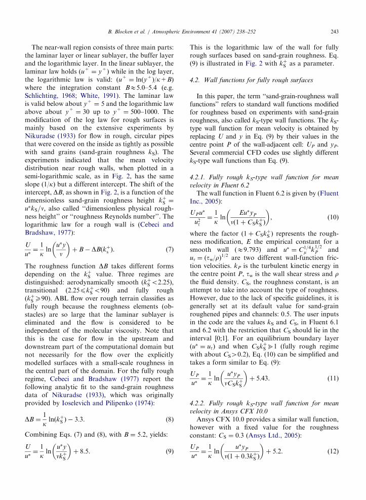
Fig. 3. Graphical representation of fitting the mean-velocity ABL

log-law inlet profile to the wall function for mean velocity in the

centre point P of the wall-adjacent cell.


In the fully rough regime (kþS490) it can berewritten as follows:

UP

u�¼

1

kln

u�yP

0:3nkþS

� �þ 5:2. (13)

4.2.3. Wall functions for k and eIrrespective of the value of kþS , the wall functions

for the turbulent quantities are generally given by

kP ¼u�2ffiffiffiffiffiffi

Cmp , (14)

�P ¼u�3

kyP

. (15)

Note that in these equations u� carries the effect of theroughness. In Fluent 6, Eq. (14) is not used but insteadthe k equation is solved in the wall-adjacent cells.

kS-type wall functions are not only used forsimulations of flow over sand-grain roughenedsurfaces. Indeed, many CFD codes including Fluent6.2 and Ansys CFX 10.0 only provide this type ofroughness modification. Consequently, CFD simu-lations over other types of rough surfaces are alsomade with kS-type wall functions. In that case, theactual roughness is characterized by an ‘‘equiva-lent’’ sand-grain roughness height kS.

5. Inconsistency in the requirements for ABL flow

simulation

The fourth requirement for ABL flow simulationmentioned in Section 2 concerns the relationshipbetween kS and y0. It provides the equivalent sand-grain roughness height for the ABL, kS,ABL. It can bederived by first-order matching (continuity of functionand its first derivative) of the ABL velocity profile (Eq.(5)) with the wall-function velocity profile in the centrepoint P of the wall-adjacent cell, as indicated in Fig. 3.

For Eqs. (9), (11), (13) a perfect match with Eq. (5)can be obtained, yielding, respectively,

kS;ABL ¼ 30y0, (16)

kS;ABL ¼9:793y0

CsðFluentÞ, (17)

kS;ABL ¼ 29:6y0 ðAnsys CFXÞ (18)

and u�ABL ¼ u� for all three cases. In Eqs. (16)–(18),the actual value of the constants (30, 9.793 and 29.6)

depends to some extent on the value of k(0.40–0.42). In all cases, kS,ABL is clearly muchlarger than the corresponding aerodynamic rough-ness length y0. As an example, for some terraintypes in the updated Davenport roughness classifi-cation, the following values are obtained: for roughopen terrain: y0 ¼ 0:1m, kS,ABLE3m; for veryrough terrain: y0 ¼ 0:5m, kS,ABLE15m; for citycentres: y0 ¼ 2m, kS,ABLE60m. Clearly, kS,ABL willoften be very large in CFD simulations in builtenvironments. Note that a perfect match betweenEq. (1) and Eqs. (9), (11), (13) cannot be achievedsince in this case u�ABL is different from u�.

To satisfy all four requirements mentioned inSection 2 is generally impossible with the kS-type wallfunctions outlined above. The main reason is that thefourth requirement, expressed by Eq. (16), (17) or(18), in combination with the third requirement(yP4kS,ABL) implies that very large (high) controlvolumes should be used, which is in conflict with thefirst requirement (high mesh resolution, hence smallyP). Note that in Fluent, the required cell height canbe limited to some extent by maximizing CS (CS ¼ 1;see Eq. (17)) but that this will often not be satisfactory.The discussion in the remainder of this paper willfocus on—but not be limited to—the relationshipkS,ABLE30y0. Then, as an example, for a grass-covered plain with a low aerodynamic roughnesslength y0 ¼ 0:03m, kS,ABL is about 0.9m and yP

should be at least equal to this value, yielding cells ofminimum 1.8m height. For larger values of y0, muchlarger (higher) cells are needed. It is clear that thisrequirement conflicts with the need for a high gridresolution near the bottom of the computationaldomain and that no accurate solutions for near-ground flow can be obtained with cell sizes so large—see also Franke et al. (2004).


6. Discussion

A typical consequence of not adhering to all fourABL flow requirements is the occurrence of unin-tended streamwise gradients in the vertical profilesof the mean wind speed and turbulence quantities(horizontal inhomogeneity) as the flow travelsthrough the computational domain. The extent ofthe streamwise gradients depends on the shape ofthe vertical inlet profiles, the downstream flowdistance, the turbulence model, the type of wallfunction, the grid resolution (yP), the roughnessheight (kS), the roughness constant (CS) and theboundary conditions at the top and outlet of thedomain. A scenario that can explain—at leastpartly—the problems observed in some previousstudies is discussed below. In the scenario the ABLflow profiles at the inlet of the domain are Eqs.(1)–(3) or Eqs. (2), (5), (6), which is commonpractice in CFD simulations of ABL flow.

Given the requirement yP4kS, the most straight-forward choice might be to apply the required highmesh resolution near the bottom of the domain andto insert a kS value (kS,ground) that is low enough tosatisfy kS,groundoyP. Generally, this value will besignificantly lower than that required for ABL flowsimulation (kS,ABLE30y0); e.g. sometimes kS ¼ y0

has been used. In this case, the change in roughnessbetween the inlet profile that is representative of theterrain upstream of the domain inlet (correspondingto kS,inlet ¼ kS,ABLE30y0) and the actual smallerground roughness in the upstream part of thecomputational domain (kS,groundo30y0) will intro-duce an IBL, in which the mean wind speed andturbulence profiles will rapidly adapt to the new andsmaller roughness, yielding, amongst others, aconsiderable acceleration of the flow near thesurface. This can explain—at least partly—theunintended streamwise gradients observed by sev-eral authors mentioned in the Introduction.

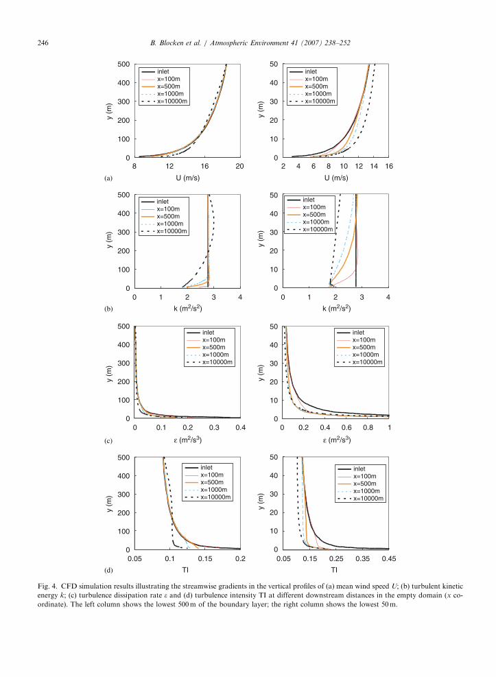
To illustrate this scenario, CFD simulations ofABL flow were performed in a 2D, empty computa-tional domain with Fluent 6.1.22. Note that a 2Dsimulation does not truly represent 3D turbulencebut that it serves the purpose of illustrating theproblem using the standard k–e model and econom-ically evaluating possible remedial measures. Thedomain has dimensions L�H ¼ 10,000� 500m. Astructured mesh was generated based on grid-sensitivity analysis, with yP ¼ 0:25m and a total of46,000 cells, equidistantly spaced in the horizontaldirection (cell length Dx ¼ 10m). The inlet profiles

are taken equal to Eqs. (2), (5), (6) with y0 ¼ 0:1mand u�ABL ¼ 0:912m s�1. At the bottom of thedomain, the standard wall functions (Eqs. (10),(15)) in the code are used, with kS,ground ¼ 0.24m(as large as possible while satisfying kS,groundoyP)and with the default roughness constant CS ¼ 0:5.Note that kS,groundokS,ABL ¼ 1.959m. As alsoindicated by Richards and Hoxey (1993), specificattention is needed for the boundary condition atthe top of the domain. Along the length of this topboundary, the values from the inlet profiles of U, k

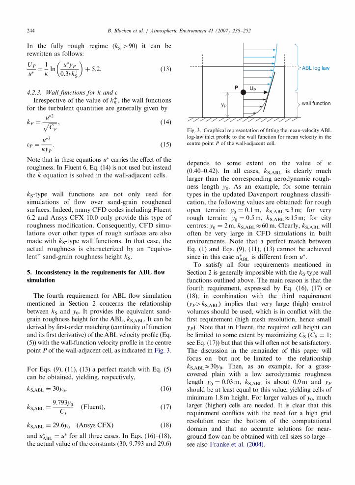
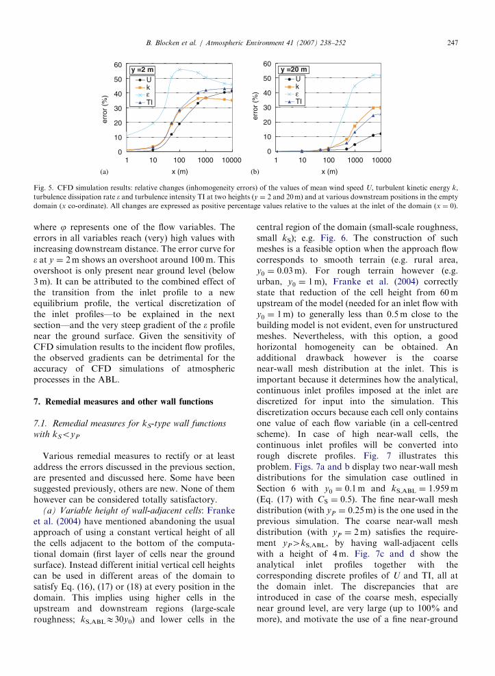
and e at this height are imposed (U ¼ 18:5m s�1,k ¼ 2:77m2 s�2, � ¼ 0:0036m2 s�3). This is done byfixing these constant values in the top layer of cellsin the domain. The application of this particulartype of top boundary condition is importantbecause other top boundary conditions (symmetry,slip wall, etc) can themselves cause streamwisegradients, in addition to those caused by the wallfunctions. At the outlet, an ‘‘outflow’’ boundary isused, which assumes no streamwise gradients at thislocation. The 2D Reynolds-averaged Navier–Stokes(RANS) equations and the continuity equation aresolved using the control volume method. Closure isobtained using the standard k–e model. Pressure–velocity coupling is taken care of by the SIMPLEalgorithm. Pressure interpolation is second order.Second-order discretization schemes are used forboth the convection terms and the viscous terms ofthe governing equations. Fig. 4 illustrates thesimulation results. The figures on the left show theprofiles from ground level up to 500m height, whilethe figures on the right only show the lowest 50m.As the profiles travel downstream, the streamwisegradients become very pronounced, particularlynear the ground surface and they exhibit the typicalcharacteristics of a developing IBL. After a con-siderable distance (about x ¼ 5000m, not shown infigure) the profiles attain a new equilibrium with thecurrent simulation parameters (i.e. turbulence mod-el, wall functions, values of yP, kS, CS and top andoutlet boundary condition). Note that changes inthese parameters will lead to similar observationsbut to different profiles. Fig. 5 illustrates the relativechange, i.e. inhomogeneity error e relative to inletprofile, for each of the variables U, k, e and TI, as afunction of downstream distance at two heights(y ¼ 2 and 20m):

e ¼ 100jðxÞ � jðx¼0Þ

jðx¼0Þ

��, (19)

ARTICLE IN PRESS

0

10

20

30

40

50

y (m

)

0

0

10

20

30

40

50

0 1

y (m

)

00

ε (m2/s3)

y (m

)

0

10

20

30

40

50

0 2 4

y (m

)

00 2 3 4

y (m

)

0

10

20

30

40

50

2 4 6 8 10 12 14

y (m

)

0

100

200

300

400

500

8 12 16

y (m

)

inletx=100mx=500mx=1000mx=10000m

U (m/s)

y (m

)

0.05

TI

0.1 0.15 0.2

TI

0.250.150.05 0.450.35

ε (m2/s3)

k (m2/s2) k (m2/s2)

500

400

300

200

100

500

400

300

200

100

500

400

300

200

100

0.60.40.2 0.8

31

U (m/s)

1620

1

0.20.1 0.3 0.4








(a)

(b)

(c)

(d)

Fig. 4. CFD simulation results illustrating the streamwise gradients in the vertical profiles of (a) mean wind speed U; (b) turbulent kinetic

energy k; (c) turbulence dissipation rate e and (d) turbulence intensity TI at different downstream distances in the empty domain (x co-

ordinate). The left column shows the lowest 500m of the boundary layer; the right column shows the lowest 50m.


ARTICLE IN PRESS

0

10

20

30

40

50

60

1 10 100 1000 10000

erro

r (%

)

Uk

TI

0

10

20

30

40

50

60

1 10

Uk

TI

y =20 m y =2 m

ε εer

ror

(%)

x (m)

100 1000 10000

x (m)(a) (b)

Fig. 5. CFD simulation results: relative changes (inhomogeneity errors) of the values of mean wind speed U, turbulent kinetic energy k,

turbulence dissipation rate e and turbulence intensity TI at two heights (y ¼ 2 and 20m) and at various downstream positions in the empty

domain (x co-ordinate). All changes are expressed as positive percentage values relative to the values at the inlet of the domain (x ¼ 0).


where j represents one of the flow variables. Theerrors in all variables reach (very) high values withincreasing downstream distance. The error curve fore at y ¼ 2m shows an overshoot around 100m. Thisovershoot is only present near ground level (below3m). It can be attributed to the combined effect ofthe transition from the inlet profile to a newequilibrium profile, the vertical discretization ofthe inlet profiles—to be explained in the nextsection—and the very steep gradient of the e profilenear the ground surface. Given the sensitivity ofCFD simulation results to the incident flow profiles,the observed gradients can be detrimental for theaccuracy of CFD simulations of atmosphericprocesses in the ABL.

7. Remedial measures and other wall functions

7.1. Remedial measures for kS-type wall functions

with kSoyP

Various remedial measures to rectify or at leastaddress the errors discussed in the previous section,are presented and discussed here. Some have beensuggested previously, others are new. None of themhowever can be considered totally satisfactory.

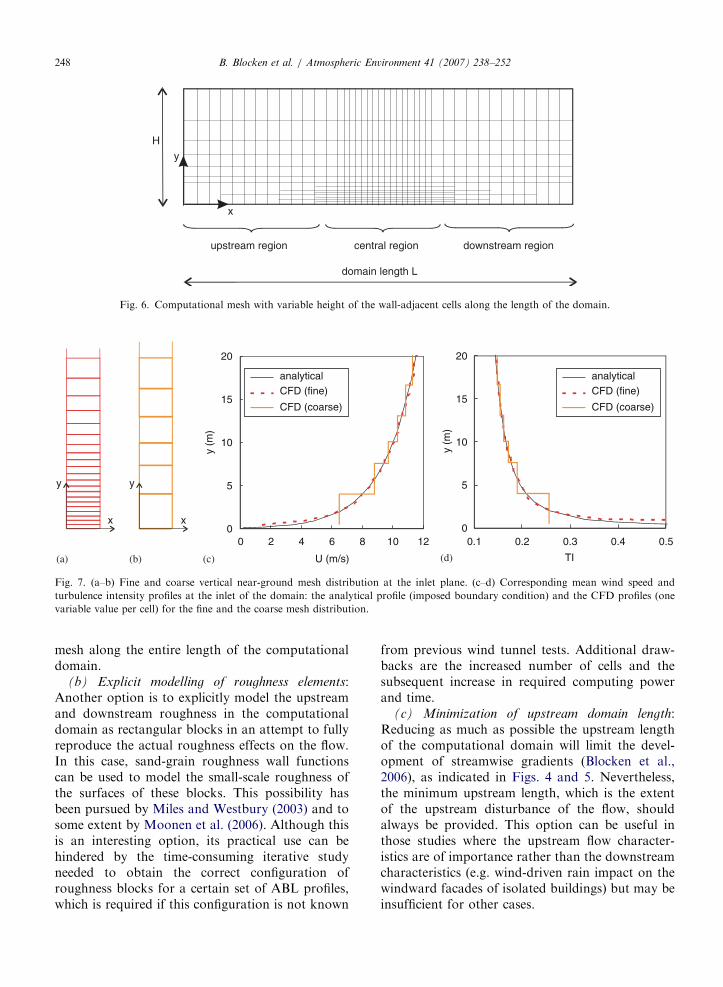
(a) Variable height of wall-adjacent cells: Frankeet al. (2004) have mentioned abandoning the usualapproach of using a constant vertical height of allthe cells adjacent to the bottom of the computa-tional domain (first layer of cells near the groundsurface). Instead different initial vertical cell heightscan be used in different areas of the domain tosatisfy Eq. (16), (17) or (18) at every position in thedomain. This implies using higher cells in theupstream and downstream regions (large-scaleroughness; kS,ABLE30y0) and lower cells in the

central region of the domain (small-scale roughness,small kS); e.g. Fig. 6. The construction of suchmeshes is a feasible option when the approach flowcorresponds to smooth terrain (e.g. rural area,y0 ¼ 0:03m). For rough terrain however (e.g.urban, y0 ¼ 1m), Franke et al. (2004) correctlystate that reduction of the cell height from 60mupstream of the model (needed for an inlet flow withy0 ¼ 1m) to generally less than 0.5m close to thebuilding model is not evident, even for unstructuredmeshes. Nevertheless, with this option, a goodhorizontal homogeneity can be obtained. Anadditional drawback however is the coarsenear-wall mesh distribution at the inlet. This isimportant because it determines how the analytical,continuous inlet profiles imposed at the inlet arediscretized for input into the simulation. Thisdiscretization occurs because each cell only containsone value of each flow variable (in a cell-centredscheme). In case of high near-wall cells, thecontinuous inlet profiles will be converted intorough discrete profiles. Fig. 7 illustrates thisproblem. Figs. 7a and b display two near-wall meshdistributions for the simulation case outlined inSection 6 with y0 ¼ 0:1m and kS,ABL ¼ 1.959m(Eq. (17) with CS ¼ 0:5). The fine near-wall meshdistribution (with yP ¼ 0:25m) is the one used in theprevious simulation. The coarse near-wall meshdistribution (with yP ¼ 2m) satisfies the require-ment yP4kS,ABL, by having wall-adjacent cellswith a height of 4m. Fig. 7c and d show theanalytical inlet profiles together with thecorresponding discrete profiles of U and TI, all atthe domain inlet. The discrepancies that areintroduced in case of the coarse mesh, especiallynear ground level, are very large (up to 100% andmore), and motivate the use of a fine near-ground

ARTICLE IN PRESS

0

5

10

15

20

TI

y (m

)

0

5

10

15

20

0 4

y (m

)

CFD (coarse)

(a) (b) (c)

y

x

y

x

analyticalCFD (fine)

U (m/s)

6 82 10 12 0.1 0.2 0.3 0.4 0.5

(d)

CFD (coarse)

analyticalCFD (fine)

Fig. 7. (a–b) Fine and coarse vertical near-ground mesh distribution at the inlet plane. (c–d) Corresponding mean wind speed and

turbulence intensity profiles at the inlet of the domain: the analytical profile (imposed boundary condition) and the CFD profiles (one

variable value per cell) for the fine and the coarse mesh distribution.

y

H

x

upstream region central region downstream region

domain length L

Fig. 6. Computational mesh with variable height of the wall-adjacent cells along the length of the domain.


mesh along the entire length of the computationaldomain.

(b) Explicit modelling of roughness elements:Another option is to explicitly model the upstreamand downstream roughness in the computationaldomain as rectangular blocks in an attempt to fullyreproduce the actual roughness effects on the flow.In this case, sand-grain roughness wall functionscan be used to model the small-scale roughness ofthe surfaces of these blocks. This possibility hasbeen pursued by Miles and Westbury (2003) and tosome extent by Moonen et al. (2006). Although thisis an interesting option, its practical use can behindered by the time-consuming iterative studyneeded to obtain the correct configuration ofroughness blocks for a certain set of ABL profiles,which is required if this configuration is not known

from previous wind tunnel tests. Additional draw-backs are the increased number of cells and thesubsequent increase in required computing powerand time.

(c) Minimization of upstream domain length:Reducing as much as possible the upstream lengthof the computational domain will limit the devel-opment of streamwise gradients (Blocken et al.,2006), as indicated in Figs. 4 and 5. Nevertheless,the minimum upstream length, which is the extentof the upstream disturbance of the flow, shouldalways be provided. This option can be useful inthose studies where the upstream flow character-istics are of importance rather than the downstreamcharacteristics (e.g. wind-driven rain impact on thewindward facades of isolated buildings) but may beinsufficient for other cases.

ARTICLE IN PRESS

0

10

20

30

1 10000

erro

r (%

)

U(NC)U(ALK)U(WSS)TI(NC)TI(WSS)

0

10

20

30

40

50

1

erro

r (%

)

U(NC)U(ALK)U(WSS)TI(NC)TI(WSS)

y =20 m y = 2 m

x (m)x (m)

10000100010010 10 100 1000

(a) (b)

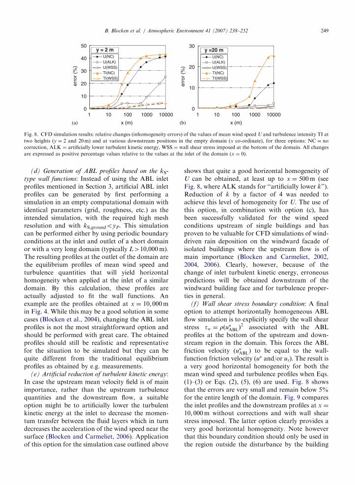
Fig. 8. CFD simulation results: relative changes (inhomogeneity errors) of the values of mean wind speed U and turbulence intensity TI at

two heights (y ¼ 2 and 20m) and at various downstream positions in the empty domain (x co-ordinate), for three options: NC ¼ no

correction, ALK ¼ artificially lower turbulent kinetic energy, WSS ¼ wall shear stress imposed at the bottom of the domain. All changes

are expressed as positive percentage values relative to the values at the inlet of the domain (x ¼ 0).


(d) Generation of ABL profiles based on the kS-

type wall functions: Instead of using the ABL inletprofiles mentioned in Section 3, artificial ABL inletprofiles can be generated by first performing asimulation in an empty computational domain withidentical parameters (grid, roughness, etc.) as theintended simulation, with the required high meshresolution and with kS,groundoyP. This simulationcan be performed either by using periodic boundaryconditions at the inlet and outlet of a short domainor with a very long domain (typically L410,000m).The resulting profiles at the outlet of the domain arethe equilibrium profiles of mean wind speed andturbulence quantities that will yield horizontalhomogeneity when applied at the inlet of a similardomain. By this calculation, these profiles areactually adjusted to fit the wall functions. Anexample are the profiles obtained at x ¼ 10; 000min Fig. 4. While this may be a good solution in somecases (Blocken et al., 2004), changing the ABL inletprofiles is not the most straightforward option andshould be performed with great care. The obtainedprofiles should still be realistic and representativefor the situation to be simulated but they can bequite different from the traditional equilibriumprofiles as obtained by e.g. measurements.

(e) Artificial reduction of turbulent kinetic energy:In case the upstream mean velocity field is of mainimportance, rather than the upstream turbulencequantities and the downstream flow, a suitableoption might be to artificially lower the turbulentkinetic energy at the inlet to decrease the momen-tum transfer between the fluid layers which in turndecreases the acceleration of the wind speed near thesurface (Blocken and Carmeliet, 2006). Applicationof this option for the simulation case outlined above

shows that quite a good horizontal homogeneity ofU can be obtained, at least up to x ¼ 500m (seeFig. 8, where ALK stands for ‘‘artificially lower k’’).Reduction of k by a factor of 4 was needed toachieve this level of homogeneity for U. The use ofthis option, in combination with option (c), hasbeen successfully validated for the wind speedconditions upstream of single buildings and hasproven to be valuable for CFD simulations of wind-driven rain deposition on the windward facade ofisolated buildings where the upstream flow is ofmain importance (Blocken and Carmeliet, 2002,2004, 2006). Clearly, however, because of thechange of inlet turbulent kinetic energy, erroneouspredictions will be obtained downstream of thewindward building face and for turbulence proper-ties in general.

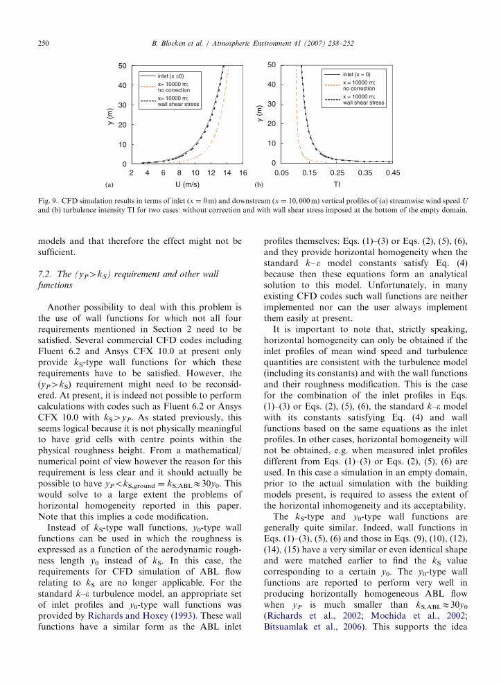
(f) Wall shear stress boundary condition: A finaloption to attempt horizontally homogeneous ABLflow simulation is to explicitly specify the wall shearstress tw ¼ rðu�ABLÞ

2 associated with the ABLprofiles at the bottom of the upstream and down-stream region in the domain. This forces the ABLfriction velocity (u�ABL) to be equal to the wall-function friction velocity (u� and/or ut). The result isa very good horizontal homogeneity for both themean wind speed and turbulence profiles when Eqs.(1)–(3) or Eqs. (2), (5), (6) are used. Fig. 8 showsthat the errors are very small and remain below 5%for the entire length of the domain. Fig. 9 comparesthe inlet profiles and the downstream profiles at x ¼

10; 000m without corrections and with wall shearstress imposed. The latter option clearly provides avery good horizontal homogeneity. Note howeverthat this boundary condition should only be used inthe region outside the disturbance by the building

ARTICLE IN PRESS

0

10

20

30

40

50

TI

y (m

)

0

10

20

30

40

50

2 4 6 8 10 12 14 16

y (m

)

inlet (x =0)

x= 10000 m; no correction

x= 10000 m; wall shear stress

inlet (x = 0)

x = 10000 m; no correction

x = 10000 m; wall shear stress

0.05 0.15 0.25 0.35 0.45

U (m/s)(a) (b)

Fig. 9. CFD simulation results in terms of inlet (x ¼ 0m) and downstream (x ¼ 10; 000m) vertical profiles of (a) streamwise wind speed U

and (b) turbulence intensity TI for two cases: without correction and with wall shear stress imposed at the bottom of the empty domain.


models and that therefore the effect might not besufficient.

7.2. The (yP4kS) requirement and other wall

functions

Another possibility to deal with this problem isthe use of wall functions for which not all fourrequirements mentioned in Section 2 need to besatisfied. Several commercial CFD codes includingFluent 6.2 and Ansys CFX 10.0 at present onlyprovide kS-type wall functions for which theserequirements have to be satisfied. However, the(yP4kS) requirement might need to be reconsid-ered. At present, it is indeed not possible to performcalculations with codes such as Fluent 6.2 or AnsysCFX 10.0 with kS4yP. As stated previously, thisseems logical because it is not physically meaningfulto have grid cells with centre points within thephysical roughness height. From a mathematical/numerical point of view however the reason for thisrequirement is less clear and it should actually bepossible to have yPokS,ground ¼ kS,ABLE30y0. Thiswould solve to a large extent the problems ofhorizontal homogeneity reported in this paper.Note that this implies a code modification.

Instead of kS-type wall functions, y0-type wallfunctions can be used in which the roughness isexpressed as a function of the aerodynamic rough-ness length y0 instead of kS. In this case, therequirements for CFD simulation of ABL flowrelating to kS are no longer applicable. For thestandard k–e turbulence model, an appropriate setof inlet profiles and y0-type wall functions wasprovided by Richards and Hoxey (1993). These wallfunctions have a similar form as the ABL inlet

profiles themselves: Eqs. (1)–(3) or Eqs. (2), (5), (6),and they provide horizontal homogeneity when thestandard k– e model constants satisfy Eq. (4)because then these equations form an analyticalsolution to this model. Unfortunately, in manyexisting CFD codes such wall functions are neitherimplemented nor can the user always implementthem easily at present.

It is important to note that, strictly speaking,horizontal homogeneity can only be obtained if theinlet profiles of mean wind speed and turbulencequantities are consistent with the turbulence model(including its constants) and with the wall functionsand their roughness modification. This is the casefor the combination of the inlet profiles in Eqs.(1)–(3) or Eqs. (2), (5), (6), the standard k–e modelwith its constants satisfying Eq. (4) and wallfunctions based on the same equations as the inletprofiles. In other cases, horizontal homogeneity willnot be obtained, e.g. when measured inlet profilesdifferent from Eqs. (1)–(3) or Eqs. (2), (5), (6) areused. In this case a simulation in an empty domain,prior to the actual simulation with the buildingmodels present, is required to assess the extent ofthe horizontal inhomogeneity and its acceptability.

The kS-type and y0-type wall functions aregenerally quite similar. Indeed, wall functions inEqs. (1)–(3), (5), (6) and those in Eqs. (9), (10), (12),(14), (15) have a very similar or even identical shapeand were matched earlier to find the kS valuecorresponding to a certain y0. The y0-type wallfunctions are reported to perform very well inproducing horizontally homogeneous ABL flowwhen yP is much smaller than kS,ABLE30y0(Richards et al., 2002; Mochida et al., 2002;Bitsuamlak et al., 2006). This supports the idea


that violating ‘‘yP4kS’’ should also be possible forkS-type wall functions. However, due to currentrestrictions in several CFD codes including Fluent6.2 and Ansys CFX 10.0, the requirement yP4kSstill has to be satisfied, and to limit horizontalinhomogeneity one has to resort to one or several ofthe remedial measures reported in Section 7.1.

8. Summary and conclusions

The accuracy of CFD simulations for atmo-spheric studies such as pollutant dispersion anddeposition can be seriously compromised whenwall-function roughness modifications based onexperimental data for sand-grain roughened pipesand channels (kS-type wall functions) are applied atthe bottom of the computational domain. This typeof roughness modification is currently present inmany CFD codes including Fluent 6.2 and AnsysCFX 10.0. The problems typically manifest them-selves as unintended changes (streamwise gradients)in the vertical mean wind speed and turbulenceprofiles as they travel through the computationaldomain (horizontal homogeneity problem). Thesegradients can—at least partly—be held responsiblefor the discrepancies sometimes found betweenseemingly identical CFD simulations performedwith different CFD codes and between CFDsimulations and measurements.

The problems are caused because it is generallyimpossible to simultaneously satisfy all four require-ments for ABL flow simulations when kS-type wallfunctions are used. The extent of the streamwisegradients depends on various simulation character-istics and settings, including the inlet profiles, theturbulence model, the type of wall functions, thenear-wall grid resolution, the roughness height andthe roughness constant.

The best solution to this problem is to alleviatethe requirement yP4kS. This can be done either byusing y0-type wall functions or using kS-type wallfunctions in CFD code formulations that allowviolating this requirement. However, at the time ofwriting this paper, several CFD codes includingFluent 6.2 and Ansys CFX 10.0 allow neither ofthese options, in which case one or more of theremedial measures mentioned in Section 7.1 shouldbe considered.

Irrespective of the type of simulation, the inletprofiles, turbulence model, wall functions and near-wall grid resolution used, it is advisable to alwaysassess the extent of horizontal inhomogeneity by a

simulation in an empty computational domain priorto the actual simulation with the obstacle modelspresent. Sensitivity tests in an empty computationaldomain are of critical importance. In addition, forevery CFD simulation it is advisable to alwaysreport not only the inlet profiles but also theincident flow profiles obtained from the simulationin the empty domain because they characterize thereal flow to which the building models are subjected.

Acknowledgements

This research has been conducted while the firstauthor was a post-doctoral research fellow of theFWO-Flanders (Research Fund—Flanders), anorganization that supports and stimulates funda-mental research in Flanders (Belgium). Theirfinancial contribution is gratefully acknowledged.The authors also wish to express their gratitude forthe valuable discussions with Dr. Jorg Franke, Dr.Alan Huber, Dr. Bob Meroney, Dr. David Banksand Ir. David Dooms.

References

Ansys Ltd., 2005. Ansys CFX-Solver, Release 10.0: Theory.

Canonsburg.

Bitsuamlak, G.T., Stathopoulos, T., Bedard, C., 2004. Numerical

evaluation of wind flow over complex terrain: review. Journal

of Aerospace Engineering 17 (4), 135–145.

Bitsuamlak, G., Stathopoulos, T., Bedard, C., 2006. Effects of

upstream two-dimensional hills on design wind loads: a

computational approach. Wind and Structures 9 (1), 37–58.

Blocken, B., Carmeliet, J., 2002. Spatial and temporal distribu-

tion of driving rain on a low-rise building. Wind and

Structures 5 (5), 441–462.

Blocken, B., Carmeliet, J., 2004. A review of wind-driven rain

research in building science. Journal of Wind Engineering and

Industrial Aerodynamics 92 (13), 1079–1130.

Blocken, B., Carmeliet, J., 2006. The influence of the wind-

blocking effect by a building on its wind-driven rain exposure.

Journal of Wind Engineering and Industrial Aerodynamics 94

(2), 101–127.

Blocken, B., Roels, S., Carmeliet, J., 2004. Modification of

pedestrian wind comfort in the Silvertop Tower passages by

an automatic control system. Journal of Wind Engineering

and Industrial Aerodynamics 92 (10), 849–873.

Blocken, B., Carmeliet, J., Stathopoulos, T., 2006. CFD

evaluation of the wind speed conditions in passages between

buildings—effect of wall-function roughness modifications on

the atmospheric boundary layer flow. Journal of Wind

Engineering and Industrial Aerodynamics, accepted for

publication.

Castro, I.P., Robins, A.G., 1977. The flow around a surface

mounted cube in a uniform and turbulent shear flow. Journal

of Fluid Mechanics 79 (2), 307–335.

ARTICLE IN PRESSB. Blocken et al. / Atmospheric Environment 41 (2007) 238–252252

Cebeci, T., Bradshaw, P., 1977. Momentum Transfer in

Boundary Layers. Hemisphere Publishing Corporation, New

York.

Davenport, A.G., 1960. Rationale for determining design wind

velocities. Journal of the Structural Division, Proceedings of

the American Society of Civil Engineers 86, 39–68.

Davenport, A.G., 1961. The application of statistical concepts to

the wind loading of structures. In: Proceedings of the

Institution of Civil Engineers, August.

Durbin, P.A., Petterson Reif, B.A., 2001. Statistical Theory and

Modelling for Turbulent Flows. Wiley, Chichester, UK.

Fluent Inc., 2005. Fluent 6.2 User’s Guide. Fluent Inc., Lebanon.

Franke, J., Frank, W., 2005. Numerical simulation of the flow

across an asymmetric street intersection. In: Naprstek, J.,

Fischer, C. (Eds.), Proceedings of the 4EACWE, 11–15 July

2005, Prague, Czech Republic.

Franke, J., Hirsch, C., Jensen, A.G., Krus, H.W., Schatzmann,

M., Westbury, P.S., Miles, S.D., Wisse, J.A., Wright, N.G.,

2004. Recommendations on the use of CFD in wind

engineering In: Proceedings of the International Conference

on Urban Wind Engineering and Building Aerodynamics. In:

van Beeck JPAJ (Ed.), COST Action C14, Impact of Wind

and Storm on City Life Built Environment. von Karman

Institute, Sint-Genesius-Rode, Belgium, 5–7 May 2004.

Gao, Y., Chow, W.K., 2005. Numerical studies on air flow

around a cube. Journal of Wind Engineering and Industrial

Aerodynamics 93 (3), 115–135.

Harris, R.I., Deaves, D.M., 1981. The structure of strong winds.

Wind engineering in the eighties. In: Proceedings of the

CIRIA Conference, Construction Industry Research and

Information Association, London, 12–13 November 1980

(paper 4).

Ioselevich, V.A., Pilipenko, V.I., 1974. Logarithmic velocity

profile for flow of a weak polymer solution near a rough

surface. Soviet Physics-Doklady 18, 790.

Jones, W.P., Launder, B.E., 1972. The prediction of laminariza-

tion with a 2-equation model of turbulence. International

Journal of Heat and Mass Transfer 15, 301.

Launder, B.E., Spalding, D.B., 1974. The numerical computation

of turbulent flows. Computer Methods in Applied Mechanics

and Engineering 3, 269–289.

Mathews, E.H., 1987. Prediction of the wind-generated pressure

distribution around buildings. Journal of Wind Engineering

and Industrial Aerodynamics 25, 219–228.

Meroney, R.N., 2004. Wind tunnel and numerical simulation of

pollution dispersion: a hybrid approach. Working paper,

Croucher Advanced Study Insitute on Wind Tunnel Model-

ing, Hong Kong University of Science and Technology, 6–10

December 2004, 60pp.

Miles, S., Westbury, P., 2003. Practical tools for wind engineering

in the built environment. QNET-CFD Network Newsletter 21

(2), 11–14.

Mochida, A., Tominaga, Y., Murakami, S., Yoshie, R., Ishihara,

T., Ooka, R., 2002. Comparison of various k–e models and

DSM applied to flow around a high-rise building—report on

AIJ cooperative project for CFD prediction of wind environ-

ment. Wind and Structures 5 (2–4), 227–244.

Moonen, P., Blocken, B., Roels, S., Carmeliet, J., 2006.

Numerical modeling of the flow conditions in a closed-circuit

low-speed wind tunnel. Journal of Wind Engineering

and Industrial Aerodynamics, in press. doi:10.1016/

j.jweia.2006.02.001.

Nikuradse, J., 1933. Stromungsgesetze in rauhen Rohren.

Forschung Arb. Ing.-Wes. No. 361.

Quinn, A.D., Wilson, M., Reynolds, A.M., Couling, S.B., Hoxey,

R.P., 2001. Modelling the dispersion of aerial pollutants from

agricultural buildings—an evaluation of computational fluid

dynamics (CFD). Computers and Electronics in Agriculture

30, 219–235.

Reichrath, S., Davies, T.W., 2002. Using CFD to model the

internal climate of greenhouses: past, present and future.

Agronomie 22 (1), 3–19.

Richards, P.J., 1989. Computational modelling of wind flows

around low rise buildings using PHOENIX. Report for the

ARFC Institute of Engineering Research Wrest Park, Silsoe

Research Institute, Bedfordshire, UK.

Richards, P.J., Hoxey, R.P., 1993. Appropriate boundary

conditions for computational wind engineering models using

the k–e turbulence model. Journal of Wind Engineering and

Industrial Aerodynamics 46&47, 145–153.

Richards, P.J., Younis, B.A., 1990. Comments on ‘‘Prediction of

the wind-generated pressure distribution around buildings’’

by E.H. Mathews. Journal of Wind Engineering and

Industrial Aerodynamics 34, 107–110.

Richards, P.J., Quinn, A.D., Parker, S., 2002. A 6m cube in an

atmospheric boundary layer flow. Part 2. Computational

solutions. Wind and Structures 5 (2–4), 177–192.

Riddle, A., Carruthers, D., Sharpe, A., McHugh, C., Stocker, J.,

2004. Comparisons between FLUENT and ADMS for

atmospheric dispersion modelling. Atmospheric Environment

38 (7), 1029–1038.

Schlichting, H., 1968. Boundary-Layer Theory, sixth ed.

McGraw-Hill, New York.

Stathopoulos, T., 1997. Computational wind engineering: past

achievements and future challenges. Journal of Wind

Engineering and Industrial Aerodynamics 67–68, 509–532.

White, F.M., 1991. Viscous Fluid Flow, second ed. McGraw-

Hill, New York.

Wieringa, J., 1992. Updating the Davenport roughness classifica-

tion. Journal of Wind Engineering and Industrial Aerody-

namics 41–44, 357–368.

Zhang, C.X., 1994. Numerical prediction of turbulent recirculat-

ing flows with a k–e model. Journal of Wind Engineering and

Industrial Aerodynamics 51, 177–201.

dx.doi.org/10.1016/j.jweia.2006.02.001

dx.doi.org/10.1016/j.jweia.2006.02.001

Documents

Blocken