Bloom and Bust: Toxic Algae’s Impact on Nearby Property Values

David Wolf

The Ohio State University

Wolf.527@osu.edu

H. Allen Klaiber

The Ohio State University

Klaiber.16@osu.edu

Selected Paper prepared for presentation at the 2016 Agricultural & Applied Economics Association Annual Meeting, Boston, Massachusetts, July 31-August 2.

Copyright 2016 by David Wolf, and H. Allen Klaiber. All rights reserved. Readers may make

verbatim copies of this document for non-commercial purposes by any means, provided that

this copyright notice appears on all such copies.

1

Abstract

Over the past decade harmful algal blooms (HABs) have become a nationwide

environmental concern. HABs are likely to increase in frequency and intensity due to rising

summer temperatures caused by climate change and higher nutrient enrichment from

increased urbanization. Policymakers need information on the economic costs of HABs to

design optimal management policies in the face of limited budgets. Using a detailed, multi-

lake hedonic analysis across 6 Ohio counties between 2009 and 2015 we show capitalization

losses associated with near lake homes between 12% and 17% rising to over 30% for lake

adjacent homes. In the case of Grand Lake Saint Marys, we find capitalization losses

exceeding $48 million for near lake homes which dwarfs the State of Ohio’s cleanup

expenditure of $26 million.

Keywords: harmful algal bloom; hedonic; blue green algae; cyanobacteria; capitalization; inland

lake

JEL Codes: Q25, Q51, Q53, Q57

2

1. Introduction

On August 2nd, 2014 the city of Toledo, Ohio issued a warning to its 500,000 metro

residents advising them not to drink, bathe in, or boil their tap water. Later that same day

approximately 60 people were hospitalized with abdominal pain, the governor of Ohio, John

Kasich, declared a state of emergency and the National Guard was called in to distribute

thousands of gallons of bottled water to residents. What was at the heart of this commotion?

Massive blue green algae(cyanobacteria) blooms which formed near the public water intake pipe.

Although not all algae is dangerous, the blooms near Toledo produced a freshwater toxin called

microcystin which can be harmful to humans and animals if ingested (Carmichael 1992).

Symptoms of cyanobacteria poisoning include skin irritation, vomiting, diarrhea, acute liver

toxicosis, gastrointestinal disturbances, fever, pneumonia, and even death.

In addition to being a public health concern, cyanobacteria blooms are becoming

increasingly expensive for water treatment facilities to manage. After an algal bloom spread 650

miles across the Ohio River in early fall of 2015, the Greater Cincinnati Water Works was

reportedly spending $7,500 a day to remove the harmful toxins (Arenschield 2015, Oct). The

Celina water treatment plant, which pumps its untreated water from Grand Lake Saint Marys

(GLSM) in Ohio, recently upgraded its facility to address worsening water conditions found at

the lake. Initial construction and installation costs for the new plant were $7.2 million while the

annual operating costs have remained steady around $500,000 over the past seven years

(Raymond 2012). The city of Celina has passed along some of these costs to consumers by

charging an additional $7.50 fee on utility bills (Miller 2015).

As a result of both health warnings and aesthetic concerns, the general public has taken

notice of deteriorating water conditions associated with harmful algal blooms (HABs). Lakeshore

residents across multiple states have reported anecdotal evidence of significant declines in their

property values with some even suggesting a 30-50% drop due to the presence of HABs

(Arenschield 2015, Oct; Rathke 2015). Highlighting the increase in public awareness of blue

3

green algae, a nationwide LexisNexis search for the keyword “blue green algae” found 304

popular press articles relating to the topic published between 2009 and 2010. This number has

steadily risen since 2009, reaching 347 in 2011 and 2012 and 438 in the 2013-2014 period.

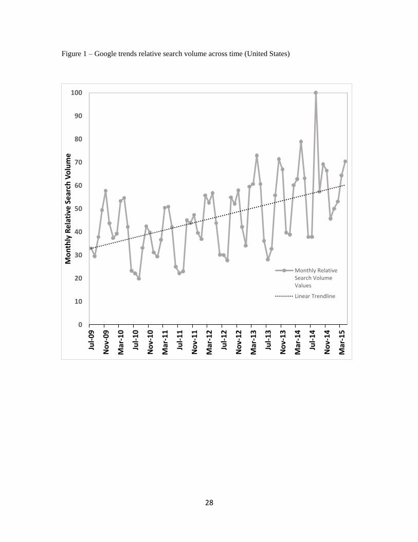
Public concern over HABs is also reflected in Google Trends data which is displayed in Figure

1.1 Google searches for the term “algal bloom” have been rising across time, with interest in the

topic appearing to be cyclical corresponding to months when algal blooms are most prevalent.

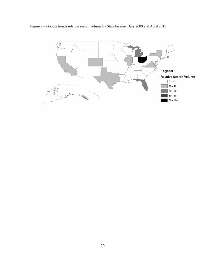
Across all 50 states, Ohio residents appear to be the most attuned to this topic, garnering a

relative search value of 100 as shown in Figure 2.

Building on the anecdotal evidence of negative property price impacts and the relatively

high level of public awareness of blue green algae in Ohio, this paper is the first to use revealed

preference housing market data to obtain direct estimates of the potential housing price

capitalization losses associated with blue green algae. To accomplish this we use a number of

inland lake housing markets scattered across Ohio combined with time-varying microcystin levels

obtained from in-lake monitoring stations to estimate hedonic models of blue green algae’s

impact on nearby housing prices. Given the large sums of ongoing public expenditure allocated

to mitigate algal blooms, it is imperative that policymakers have actual damage (cost) estimates

associated with harmful algal blooms (HABs) as an input into cost-benefit decision making when

confronting this public health and amenity threat.

Using data on microcystin concentrations associated with HABs for four inland lakes in

Ohio between 2009 and 2014 we estimate a series of first-stage hedonic models to examine the

impact of HABs on surrounding property prices. Our primary findings show that housing values

decline between 12% and 17% when microcystin concentration levels surpass the no-drinking

threshold set by the World Health Organization. This finding is robust to numerous spatial and

temporal constraints and the manner in which microcystin values are assigned to housing units.

1 Google Trends data were collected between July 1st, 2009 and May 1st, 2015. This time frame corresponds with the sample time period.

4

However, we find little evidence that housing values respond to marginal changes in microcystin

after reaching this threshold. This suggests that policies designed to eliminate, rather than

constrain, microcystin levels are likely to have greater benefits to surrounding residents in terms

of property price impacts. However, this result could also suggest a disconnect between

potentially increasing public health concerns as microcystin levels increase and nearby residents

perceptions of these risks.

The remainder of the paper is structured as follows. The next section briefly reviews the

literature on water quality as it relates to property values. Section 3 describes the housing and

HAB data used in our analysis. Section 4 introduces our hedonic specification and is followed in

section 5 by our estimation results. Finally, section 6 concludes.

2. Linking property price impacts to water quality

There exists a significant volume of empirical literature devoted to valuing changes in water

quality, with eutrophication cited as one of the primary catalysts causing a shift in water

conditions (Boyle, Poor and Taylor 1999; Bejranonda, Hitzhusen and Hite 1999; Hill, Pugh and

Mullen 2007; Smeltzer and Heiskary 1990). Eutrophication occurs in lakes when there is an

excessive amount of nutrients present. Although nutrient levels rise naturally as lakes age,

eutrophication can also be a direct consequence of human behavior. Agricultural run-off, poorly

managed septic systems and increased housing development can lead to increased algal growth.

When algal densities reach extreme levels a thick mat of algae will often envelop the surface of

the water, preventing sunlight from reaching the bottom of the lake. Aquatic species that are

dependent on this sunlight will begin to die off which in turn can shift the fundamental structure

of the ecosystem (Smith, Tilman and Nekola 1999).

Increased algal growth has also been known to negatively affect lakeshore communities

by decreasing the recreational and aesthetic benefits gained from interacting with a nutrient-rich

body of water (Bejranonda, Hitzhusen, and Hite 1999). Large algal blooms will often cause the

5

color of the water to turn green and can produce offensive odors when they start to decay.

Determining the appropriate variable to model the eutrophication process and to use as a proxy

for water quality, however, has not been rigorously established in the literature (Holly, Boyle and

Bouchard 2000; Poor et al. 2001; Egan, et al. 2009).

Although a wide spectrum of variables have been used as a proxy for water quality,

Secchi depth is perhaps the most frequently used and accepted. Studies using Secchi depth

typically conclude the following two results. First, homeowners/lake-users are willing to pay

(WTP) more to live near/use a lake if it is less turbid, ceteris paribus (Gibbs et al. 2002; Egan et

al. 2009). The relationship between Secchi depth and WTP appears to be nonlinear, however,

since WTP estimates increase at a decreasing rate as Secchi depth increases (Ge, Kling and

Herriges 2013). Intuitively this suggests homeowners and lake-users are WTP more to improve

the water quality of a dirty lake than a clean lake (Tait et al. 2012). Policies aimed at improving

water quality are therefore considered less valuable than similar interventions that aim to prevent

water quality degradation of a similar magnitude from occurring.

Second, researchers have discovered the gains from improved water quality are spatially

limited and vary depending on the size of and distance from the water body in question

(Jørgensen et al. 2013). Capitalization estimates derived from a one foot increase in Secchi

depth, for example, were found to be almost 8 times larger for lakefront properties than for non-

lakefront properties. These estimates also declined monotonically as distance from the affected

water body increased and converged to 0 at distances greater than 1,000 meters (Walsh, Milon

and Scrogin 2011). The size of the lake is also an important factor to consider when determining

the size of the gains produced from an increase in water quality. Lakefront property values have

been found to be more susceptible to changes in water conditions when they are located near

larger lakes, holding all else equal (Boyle, Poor and Taylor 1999; Gibbs et al. 2002; Walsh, Milon

and Scrogin 2011).

6

Recently a number of other measures, besides Secchi depth, have emerged in the hedonic

literature to capture water quality. Poor et al. (2007) used measures of suspended solids and

dissolved nitrogen as a proxy for ambient water quality in Maryland, while others have used lake

depth (Bejranonda, Hitzhusen and Hite 1999), fecal coliform (Leggett and Bockstael 2000), pH

(Tuttle and Heintzelman 2015) or a water index constructed from a number of physical and

chemical measures (Ge, Kling and Herriges 2013). Most of these studies find a robust negative

relationship between housing/land values and worsening water conditions. This suggests that

although Secchi depth is an important indicator of a water body’s health, it is not the only

variable that can be used as a proxy for water quality.

Despite the significant amount of research dedicated to valuing changes in water quality,

very few studies have directly valued the impact of toxic algae on economic behavior. No studies,

to our knowledge, have obtained housing capitalization estimates for blue green algae using

revealed preference data. The need for such valuation estimates is increasing due to the rise of

blue green algae and other HABs globally (Anderson 1994; Hallegraeff 1993). HABs are

becoming increasingly problematic for communities worldwide due to excessive nutrient loadings

coupled with more favorable growth conditions resulting from climate change (Robson and

Hamilton 2003; Mooij et al. 2005).

Climate change and rising average summer temperatures have promoted HAB growth via

three channels. First cyanobacteria grow at a much faster rate than other phytoplankton when

temperatures rise above the 23 degrees Celsius mark, making it difficult for non-toxic algae to

compete (Joehnk et al. 2008). Water columns also become more stratified when temperatures rise.

This in turn favors more buoyant algae (i.e. cyanobacteria) since these algae will rise to the

surface of the water and prevent sunlight from reaching less buoyant algae below (Huisman et al.

2004). Last climate change has altered weather patterns around the world. Areas that are less

cloudy and have lower wind speeds will tend to have greater water column stratification which, as

previously mentioned, gives an advantage to cyanobacteria (Joehnk et al. 2008).

7

Cyanobacteria are well adapted to survive in a variety of climates but the value they

remove from communities is not well understood. The few studies that have attempted to value

changes in cyanobacteria levels have implemented contingent valuation (CV) methods, travel cost

models or choice experiments. Hunter et al. (2012) elicit WTP estimates for a reduction in

morbidity risk due to a reduction in cyanobacteria using survey data collected from residents of

two towns located near Loch Leven in Scotland. The results from this study suggest that each

household is willing to pay approximately £10 a year to reduce the annual number of risky days

by half. However approximately 20% of the respondents had a WTP value of 0 and indicated that

the “polluter should pay” (Hunter et al. 2012). Kosenius (2010) set up a choice experiment where

respondents were asked to choose between four different policies that would either improve water

clarity, reduce the occurrence of cyanobacteria blooms, reduce the quantity of coarse fish or

improve local aquatic vegetation in the Gulf of Finland. On average improvements in water

clarity were considered the most important followed by a reduction in the occurrence of

cyanobacteria blooms.

Excessive amounts of cyanobacteria can also disrupt recreational activities. Using a rich

set of survey data, which included responses from 8,000 Iowa households spanning 129 lakes,

Egan et al. (2009) find that cyanobacteria and phytoplankton levels are the most important pair of

water quality measures to supplement with Secchi depth to determine a recreators’ optimal

location choice. Their results also suggest that higher concentrations of cyanobacteria, while

holding all other water quality measures constant, will reduce the likelihood of a person visiting a

lake.

The above studies consistently show that high levels of cyanobacteria impact lake-users’

decision-making process. However all of the aforementioned work depends on CV or travel-cost

models to elicit WTP estimates for recreation behavior or use proxies that are more general

measures of lake quality rather than specific HAB indicators. We fill this gap in the literature by

providing the first set of hedonic-based valuation estimates for blue-green algae.

8

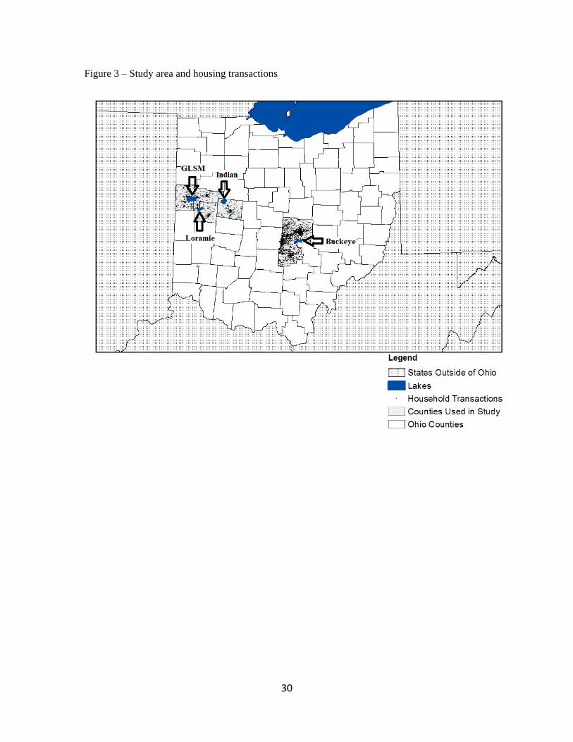
3. Data

Our study area consists of 6 counties surrounding 4 inland Ohio lakes highlighted in Figure 3.2

These lakes were specifically chosen due to an extensive set of time-varying water quality

monitoring data as well as the availability of detailed housing transactions data available from

county auditors. Given the large number of inland lakes across the country that are facing

microcystin contamination, these lakes provide a platform to estimate potential capitalization

losses that could be experienced across other inland lakes as climate change combined with

increased nutrient runoff exacerbates the frequency of HABs moving forward.

Housing transactions data were collected from six different county auditor websites

across Ohio including Auglaize, Fairfield, Licking, Logan, Mercer and Shelby counties. This data

includes historic sales information and select structural characteristics for each property sold

between July 2009 and April 2015. Depending on county, additional housing characteristics were

obtained from CDs provided by county auditors. We restricted our analysis to homes identified as

single family, omitting potential multi-family dwellings as is standard in much of the hedonic

literature.

In addition to focusing on single family homes, houses that were sold more than once

during the same year were removed to eliminate potential house flippers. Delinquent and vacant

properties were also eliminated in an attempt to remove unobservable characteristics that are

likely associated with these properties. Houses with extreme physical characteristics (i.e. any

observation with a covariate value in the 1st or 99th percentile) were labeled as outliers and

excluded from our final sample. Finally, single family residences that were sold for less than

$50,000 or had a price per square foot value less than $40/foot were removed to eliminate

potential non-arms-length transactions

2We omitted Perry County, which is adjacent to Buckeye lake due to limited GIS and housing data..

9

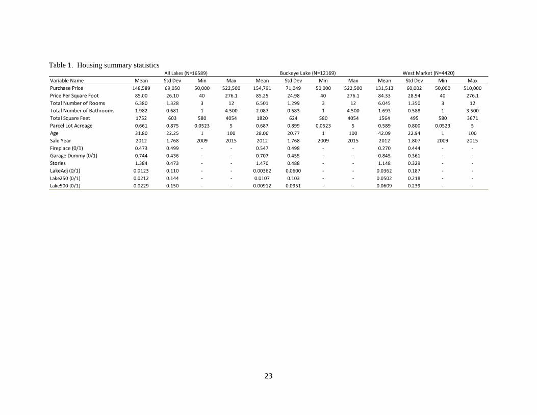
Summary statistics for our cleaned sample of 16,589 housing transactions are shown in

Table 1 for both the whole sample as well as subsamples of lakes used in our subsequent analysis.

The average house sold in our sample was valued at approximately $148,589, had 1752 square

feet, one and a half stories, a garage, a fireplace, and was 32 years old. The characteristics of

houses vary significantly across inland lake housing markets as shown in additional columns of

Table 1. Houses near Buckeye Lake were on average worth $23,000 more than the homes sold in

Ohio’s west market. Houses near GLSM, Indian Lake and Lake Loramie were more likely to

have a garage, were older, and had smaller lot sizes than homes located near Buckeye Lake.

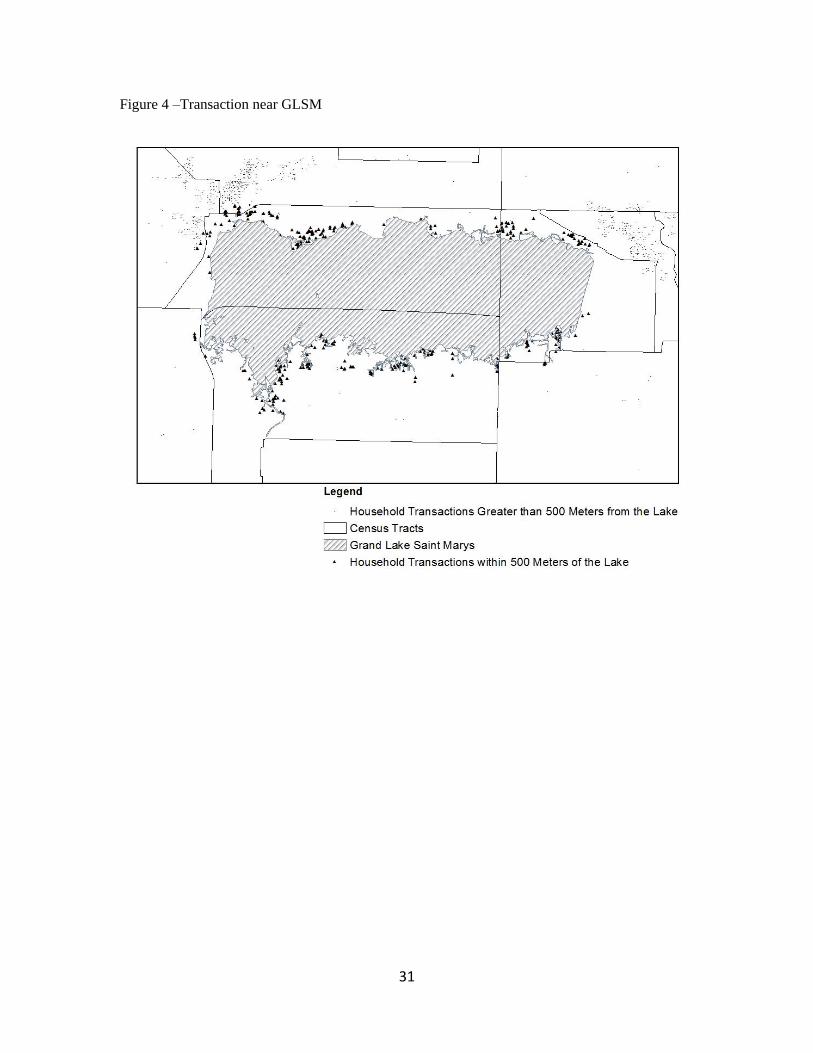
Having assembled housing transactions data, we georeferenced each transaction to a

spatial location using parcel shapefiles collected from either county GIS maps or engineering

departments. Importantly, the use of micro-level GIS data to identify the locations of homes sold

allows us to form spatially explicit measures of lake proximity which have been shown in the

prior literature to play an important role in determining highly localized capitalization effects of

lake quality. Figure 4 provides an example of parcel proximity to lakes and highlights parcels

located within 500 meters of GLSM

To identify lake proximity measures, we obtained lake shapefiles from the USGS’s

National Hydrography Dataset, along with census tract shapefiles which were overlaid onto the

parcel shapefiles using ArcGIS. This process enabled us to attach additional spatial characteristics

to each house including distance to lake as well as census tract identifiers. We assigned homes

into discrete distance bands surrounding lakes. Lakefront properties were defined based on

parcels located within 20 meters of a lake. We defined additional bands at the 250 and 500 meter

cutoffs with properties outside these bands in a remaining non-lake category.3 Summary statistics

for these measures are shown in the second panel of Table 1.

3Adding a continuous measure of distance/inverse distance to our model specification did not qualitatively change any of the study’s findings.

10

In the first panel of Table 1 we present information on the number of housing

transactions near each lake. Approximately 5% of the sample consists of homes that were sold

within 500 meters of a lake: 1.2% of the properties were sold within 20 meters of a lake, 2.1%

were located between 20 and 250 meters of a lake, and 2.3% were located between 250 and 500

meters of a lake. The relatively small increases between each distance band does not come as a

surprise since all of the lakes used in this study come from rural areas of Ohio. In the right panel

of Table 1 we separate housing transactions by lake. There are more lakefront and l near lake

homes sold near GLSM, Indian Lake and Lake Loramie than near Buckeye Lake. This likely

reflects the size of the lakes with the surface area for Buckeye Lake only 3,136 acres whereas the

combined surface area for the three aforementioned lakes is 18,647 acres.

Cyanobacteria data were collected from the HAB division of the Ohio EPA, Ohio’s

Public Water Systems, the Citizen Lake Awareness and Monitoring (CLAM) database and from

the Ohio Department of Natural Resources. All of these institutions measured the density of

harmful algae by recording microcystin, cylindrospermopsin and/or saxitoxin concentration

levels. Since microcystin are the most commonly produced freshwater toxin/by-product of

cyanobacteria, it was used as a proxy for blue-green algae (Chorus and Bartarm, 1999). Of the

four lakes used in this study, Buckeye and GLSM were the most frequently sampled. GLSM

contained 792 readings while Buckeye Lake had 334. Indian Lake and Lake Loramie were less

frequently tested only having 41 and 16 microcystin samples taken, respectively. Most of the

sample locations within each lake did not have data for all years (2009 – 2014), but for the years

that were available multiple samples were usually taken during each of the summer and fall

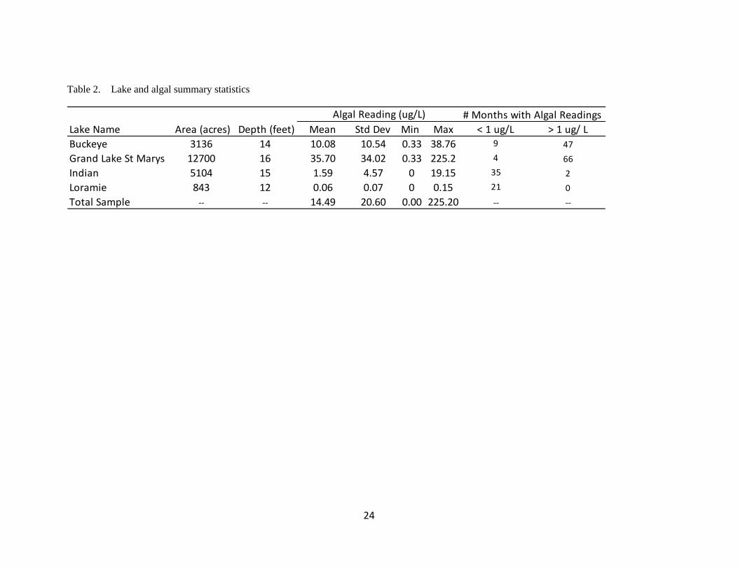
months (June-November). Table 2 displays microcystin summary statistics for each lake.

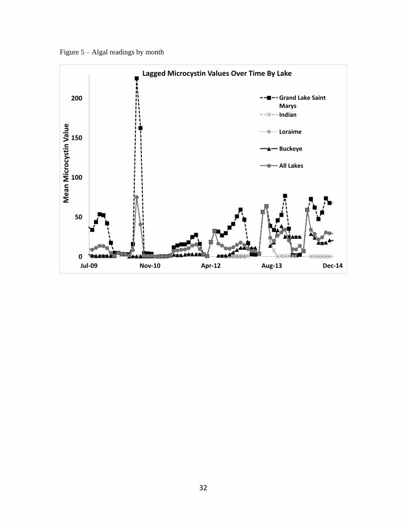
Algal condition across the four lakes in our sample exhibit substantial heterogeneity.

GLSM and Buckeye Lake tend to be the “dirtiest”. Their average microcystin concentration levels

are well above the 1 ug/ L, no drinking threshold set by the World Health Organization (WHO),

with GLSM’s average exceeding the WHO’s 20 ug/L no contact threshold (World Health

11

Organization 2003)4. The other two lakes are relatively clean with both having some samples

where no microcystin was detected in the water. A significant amount of within lake variation

exists as well which is central to our hedonic identification. GLSM and Buckeye Lake both have

at least 4 months of algal readings below the 1 ug/L threshold despite having individual algal

readings near 200 ug/L in other months. Indian Lake, on the other hand, is the opposite of GLSM

and Buckeye Lake. Most of the monthly algal values are well below the WHO’s 1 ug/L threshold,

while there are only a few months with algal blooms. Finally, Lake Loramie did not exhibit a

significant amount of within variation in water quality with all of its monthly algal readings

below the 1 ug/L threshold.

To attach microcystin levels to housing transactions we examined a number of temporal

aggregates of recent microcystin observations. Since the sale price of a home is typically

determined 30-60 days before the actual sale date occurs, we used the mean of all microcystin

samples taken two months preceding the month of the sale as the primary proxy for algal

conditions on each lake.5 If there were no microcystin readings taken within 2 months of the sale,

the temporal lag used would extend an additional month until a microcystin reading was available

up to 6 months prior to the sale6. If there were no readings taken within 6 months of the sale

month, however, the transaction was excluded from the sample due to missing data.7 Summary

statistics for algae levels associated with transactions are shown in Table 2 and reflect the overall

heterogeneity in lake conditions discussed previously. A time trend, depicting how microcystin

values varied across seasons is provided in Figure 5.

4 The Ohio EPA implemented a similar set of guidelines in 2014 (Raymond, 2014). 5 Microcystin readings taken during the month of the sale were removed from consideration to

eliminate any possibility that future algal conditions were used to predict the market value of a

home 6 For robustness we also examined using a 6 month average. While we see some attenuation of

results likely due to measurement error arising from algae aggregation, results are qualitatively

similar to our primary results presented below. 7 Results are robust when the sample is restricted to using only transactions with a microcystin

reading taken within 2 months of the sale month.

12

4. Identification of Algae’s Impact on Housing Prices

Econometric identification of the capitalization impacts of microcystin on nearby housing prices

follows the familiar first-stage hedonic logic (Rosen 1974). We assume that utility maximizing

residents bid on houses with the highest bid accepted by sellers resulting in housing transactions.

Modeling the equilibrium price that arises from this process produces the familiar first-stage

hedonic regression given by:

(1) ln 𝑃𝑖𝑗𝑡 = 𝛼0 + 𝜶𝟏𝑿𝒊 + 𝜶𝟐𝒁𝒋 + 𝜶𝟑𝒀𝒕 + 𝜶𝟒𝑴𝒕 + 𝜶𝟓𝑳𝒂𝒌𝒆𝒊𝒕 + 𝜖𝑖𝑗𝑡

where we have specified the first stage regression as a semi-log specification with the price of

house 𝑖 sold in location 𝑗 during time period 𝑡 given by 𝑃𝑖𝑗𝑡. House specific structural attributes

are given by 𝑿𝒊, dummy variables controlling for neighborhood-specific, time-invariant

characteristics are given by 𝒁𝒋, time specific dummy variables are represented by 𝒀𝒕 and 𝑴𝒕

where 𝒀𝒕 are year-specific dummy variables and 𝑴𝒕 are month-specific dummy variables, 𝜶 are

vectors of parameters to be estimated and 𝜖𝑖𝑗𝑡 is an idiosyncratic error term. Our key variables of

interest are spatially and temporally varying measures of lake quality represented by 𝑳𝒂𝒌𝒆𝒊𝒕

where the subscripts highlight that this variable varies by house and time.

Our use of distinct lakes raises several challenging issues in our estimation of the hedonic

equation in (1). The first of these concerns the source of algal variation needed for identification.

One approach is to assume that changes in algal conditions have the same impact on all lake

adjacent and lake community properties. This can be modeled using (2):

(2) ln 𝑃𝑖𝑗𝑡 = 𝛼0 + 𝜶𝟏𝑿𝒊 + 𝜶𝟐𝒁𝒋 + 𝜶𝟑𝒀𝒕 + 𝜶𝟒𝑴𝒕 + 𝛼5𝐿𝑎𝑘𝑒𝐴𝑑𝑗𝑖 + 𝛼6𝑁𝑒𝑎𝑟𝐿𝑎𝑘𝑒𝑖 +

𝛼7𝐴𝑙𝑔𝑎𝑒𝑖𝑡 ∗ (𝐿𝑎𝑘𝑒𝐴𝑑𝑗𝑖 + 𝑁𝑒𝑎𝑟𝐿𝑎𝑘𝑒𝑖)+ 𝜖𝑖𝑗𝑡.

Equation (2) differs from equation (1) by decomposing the 𝑳𝒂𝒌𝒆𝒊𝒕 term into three different

components. The first two terms—𝐿𝑎𝑘𝑒𝐴𝑑𝑗𝑖 and 𝑁𝑒𝑎𝑟𝐿𝑎𝑘𝑒𝑖—control for any benefits that are

derived from being located next to or near a lake. We specify two, mutually-exclusive proximity

13

variables here to separate the adjacency effect from the lake community effect. Any capitalization

that accrues from being adjacent to a lake will be captured by the 𝛼5 coefficient, while 𝛼6

captures the remaining lake proximity effect that may be present for non-adjacent homes located

within 500 meters of a lake but non-adjacent. The final term in equation (2) is our primary

variable of interest. It is an interaction between a time-varying indicator variable for microcystin

(𝐴𝑙𝑔𝑎𝑒𝑖𝑡) and an indicator for any home located within 500 meters of a lake formed as the union

of the indicator variables 𝐿𝑎𝑘𝑒𝐴𝑑𝑗𝑖 and 𝑁𝑒𝑎𝑟𝐿𝑎𝑘𝑒𝑖. This term represents a single average effect

of worsening algae conditions on lake adjacent and near lake property values.

Although equation (2) is useful in capturing microcystin’s overall effect, it does not allow

us to examine spatial heterogeneity that algae is likely to have on near lake and lake adjacent

prices. To further investigate this issue we modify equation (2) to allow for this possibility:

(3) ln 𝑃𝑖𝑗𝑡 = 𝛼0 + 𝜶𝟏𝑿𝒊 + 𝜶𝟐𝒁𝒋 + 𝜶𝟑𝒀𝒕 + 𝜶𝟒𝑴𝒕 + 𝛼5𝐿𝑎𝑘𝑒𝐴𝑑𝑗𝑖 + 𝛼6𝐿𝑎𝑘𝑒250𝑖 +

𝛼7𝐿𝑎𝑘𝑒500𝑖 + 𝛼8𝐿𝑎𝑘𝑒𝐴𝑑𝑗𝑖 ∗ 𝐴𝑙𝑔𝑎𝑒𝑖𝑡 + 𝛼9𝐿𝑎𝑘𝑒250𝑖 ∗ 𝐴𝑙𝑔𝑎𝑒𝑖𝑡 + 𝛼10𝐿𝑎𝑘𝑒500𝑖 ∗

𝐴𝑙𝑔𝑎𝑒𝑖𝑡+ 𝜖𝑖𝑗𝑡

There are once again several terms in equation (3) that account for the impact various measures of

proximity to a lake have on property values. 𝐿𝑎𝑘𝑒𝐴𝑑𝑗𝑖 is an indicator variable indicating whether

or not a property is located on the shoreline while 𝐿𝑎𝑘𝑒250𝑖 and 𝐿𝑎𝑘𝑒500𝑖 are mutually

exclusive distance bands each representing different distance “donuts”, in meters, away from the

lake. The key variables of interest are the interaction terms between the time varying 𝐴𝑙𝑔𝑎𝑒𝑖𝑡

variable and the various lake proximity measures.

The second issue we face is the longstanding concern in the hedonic literature over the

appropriate extent of market (Michaels and Smith 1990; Goodman and Thibodeau 2002). Given

that our data are associated with spatially noncontiguous lakes, there are a variety of potential

approaches to examining this issue. The simplest approach is to simply estimate a version of

equation (2) with pooled data accounting for shifts in the hedonic price function across space and

14

time through fixed effects. This approach ensures that identification for algae covariates arises

due to both within lake and between lake variation while exploiting a large reservoir of housing

transactions to help identify additional covariates in the hedonic specification.

An alternative extent of market arises if one focuses only on specific subsets of lakes.

When dividing the housing market by more specific localities a natural breakpoint is to consider

the lakes of GLSM, Loramie and Indian as one market and Buckeye as another. For markets

containing lakes with algal readings both above and below key toxicity thresholds identification

is still achieved through within and between lake variation in algal readings. Finally, a third

alternative is to focus exclusively on individual lakes that have both experienced algal

fluctuations and contain significant nearby housing transactions needed for identification. In our

sample, this restricts our analysis to Buckeye and GLSM.

Buckeye Lake and GLSM fulfill the stringent data requirements needed to test this third

alternative because of the consistent water quality sampling that has occurred at both lakes, with

each lake having over 300 samples taken during our study’s time period. One limitation in

running this analysis, however, is the ability to estimate spatially heterogeneous proximity effects

associated with algae. Due to GLSM’s consistently poor water conditions, there were only two

lakefront properties sold when algae conditions were below the 1 ug/L threshold. These two

observations are not sufficient to separately identify the effect of being close to a lake with the

loss in value due to higher algal concentrations. Subsequently we provide estimates only using

equation (2) for each individual lake. We present results for all three extent of market definitions

in the following section.

5. Results

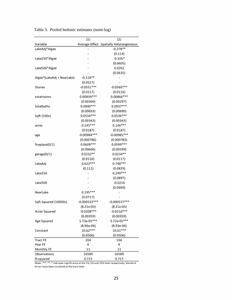
Estimation results for two base specification using a pooled dataset of all lakes based on

equations (2) and (3) are shown in Table 3. The first specification reports estimation results

based on equation (2), while the second specification allows the algal coefficient to vary across

15

space using the functional form describe in equation (3). Both specifications include census tract,

year, and monthly fixed effects.8 Census tract effects control for baseline differences across

space such as school quality or proximity to urban areas. Year fixed effects control for shifts in

the hedonic equilibrium due to appreciation or other time-varying but spatially uniform impacts.

Finally, month fixed effects control for potential seasonality in housing prices. Given that our

primary focus centers on lake quality impacted by algae, the inclusion of month fixed effects

helps to absorb differences in lake home sales between colder winter months and warmer

summers.

Examining results for each specification, housing covariates have the expected signs and

significance suggesting that the hedonic is reliably capturing baseline housing features. Housing

values increase at a decreasing rate as square footage and lot size increase. Adding an additional

bathroom to a house adds considerably more value to a property than if the space were used

instead for an additional room. Adding an additional story to a house, while holding the square

footage constant, slightly reduces the value of a home. This could be capturing some of the higher

annual heating and cooling costs that are associated with multi-story homes.

Examining lake covariates in more detail, the first column of results reveals that lake

adjacent homes located within 20 meters of a lake are approximately 86%9 higher valued than

non-adjacent homes. As expected, homes further away, yet within 500 meters, maintain a

capitalization premium although this premium decreases to approximately 22%. Turning

attention to our key algae variable, we find a negative and significant capitalization effect of algae

contamination of 12.52%.

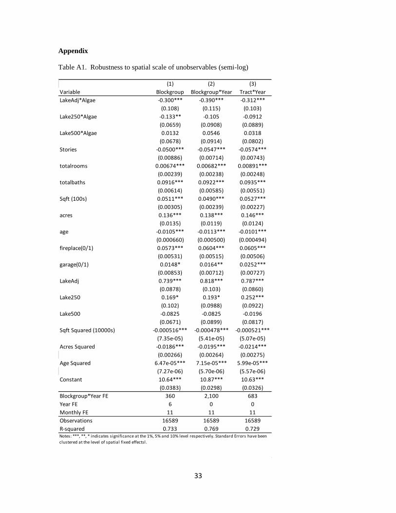
8Additional model specifications using census blockgroup, census blockgroup by year and census

tract by year fixed effects to examine the role of spatially and temporally varying unobservables

on our primary algae estimates (Abbott and Klaiber 2010). We show these results in appendix

Table A1. 9Dummy variable estimates presented in the text have been corrected using the technique

suggested by (Halvorsen and Palmquist 1980).

16

Column 2 shows results where algae impacts are allowed to vary by lake proximity. It is

clear from these results that crossing the 1 ug/L microcystin threshold significantly reduces the

value of lakefront and near lake properties. Lakefront properties appears to be the most affected

by changes in algae concentrations, losing approximately 32% of their value. Houses located

between 20 and 250 meters are also negatively impacted by increased algal density, but to a lesser

extent, losing around 11% of their value. However, when examining homes between 250 and 500

meters we no longer find a significant impact of algae contamination. This suggests that the

impact of poor water quality driven by algae contamination is spatially limited to near lake

properties.

Extent of market

To examine the role of market extent we split the sample into two groups as described in section

4. Houses located in Auglaize, Mercer, Logan and Shelby County are grouped together and form

the “West” market, while observations from Fairfield and Licking County form the “Buckeye”

market. Hedonic results from each market estimated independently are displayed in Table 4.

Results indicate there is a significant amount of heterogeneity present across housing markets.

The premium associated with living near Buckeye Lake is much larger, regardless of which

distance band a home is located in compared to the premium associated with homes in the West

market. This divergence likely reflects the heterogeneous quality of the lakes and the surrounding

amenities that they support.

In addition to different lake proximity impacts we also see evidence that the capitalized

value of structural housing attributes is slightly different across markets. While generally the

same significance and sign, magnitudes vary slightly. This difference is much more pronounced

when examining lake and algae specific covariates. Lakefront homes in the west market lose an

additional 24.5% in value as compared to their counterparts on Buckeye when algae is above 1

ug/L. This large drop in property values in the West market removes nearly half of the premium

17

that is typically associated with lakefront homes. However, the effect of algae on housing values

appears to extend further in the Buckeye market than in the western market. Homes within 250

meters of Buckeye Lake lose 19.1% of their value when water conditions worsen. This is almost

4% more than their counterparts in the western market.

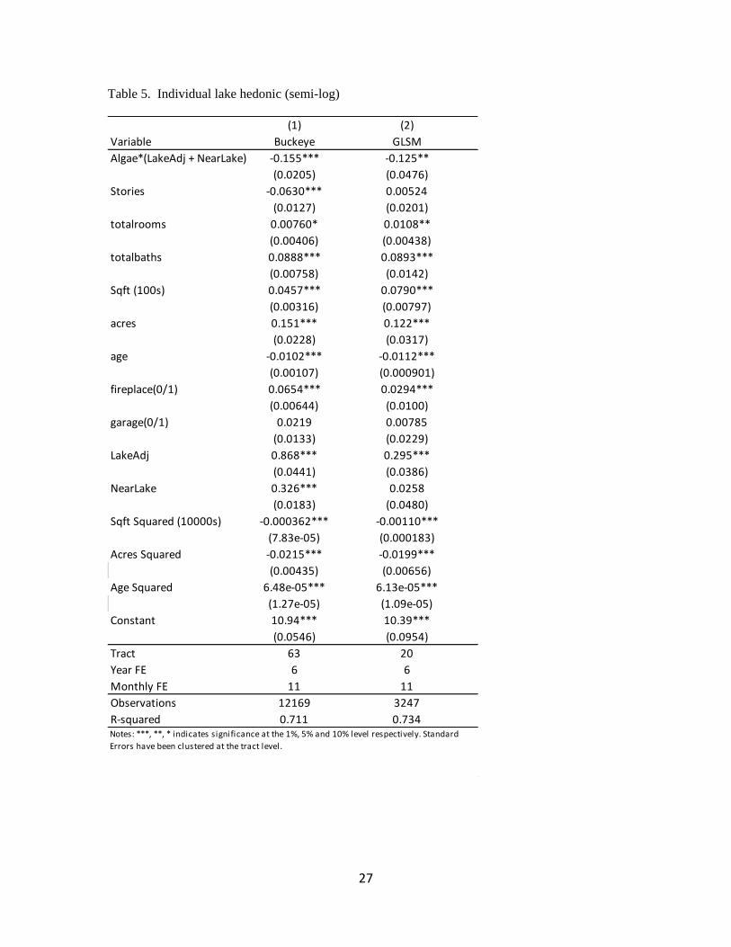
To examine a more restrictive extent of market we report results for individual lake

markets in Table 5. We estimate Buckeye Lake and GLSM individually as described in section 4.

The results in Table 5 match well with what has already been discussed. Surpassing the 1 ug/L

threshold reduces property values between 17% and 13%, respectively. The effect is

heterogeneous across lakes, with Buckeye residents being more adversely impacted by water

quality changes than GLSM residents. The distance band coefficients once again show that

quality of the lakes are heterogeneous, with Buckeye Lake being more expensive to live near. The

larger algal coefficients associated with transactions located near Buckeye Lake could be a

consequence of people’s perception of both lakes. GLSM has often been in the news over the past

several years due to poor water conditions (Arenschield 2015, Oct; Devito 2015; Henry 2011;

Egan 2014). Buckeye Lake, on the other hand, has only recently started to experience water

quality issues.

6. Discussion

State and local governments across the United States are paying closer attention to cyanobacteria

blooms. According to a survey sent out to all 50 states in 2014 by the Resource Media and

National Wildlife Federation, 71% of responding states said harmful algal blooms (HAB) were

either a “somewhat serious” or “very serious” problem. Almost half of the respondents also said

they were actively monitoring cyanobacteria levels at lakes that experienced problems with HABs

in the past (Resource Media 2014). Findings from the EPA`s 2007 National Lakes Assessment

survey support this widespread level of concern. 378 of the 1,156 lakes sampled nationwide had

18

detectable levels of microcystin. This suggests approximately one out of every three lakes

nationwide have microcystin present (EPA 2009).

Several states have taken action in response to this spread of HABs by funding lake

restoration projects. These projects have attempted to curb further toxic algal growth by dredging

sediment from the lake bottom (Barbosa 2013), creating new wetlands to filter out toxins (Devito

2015) and implementation of more stringent fertilizer restrictions to reduce the amount of runoff

that occurs (Miller 2012). Lake restoration projects can be very costly and do not ensure the

underlying problem will be eliminated. The Ohio EPA, for example, spent over $26 million

chemically treating and dredging Grand Lake Saint Marys. Despite these significant efforts many

still consider GLSM to be the poster child for HABs (Arenschield 2015, Oct).

To combat the environmental and health damages from microcystin local policymakers

face budgetary constraints given limited funding and competing demands on scarce resources. To

aid policymakers, it is important that they are aware of real costs and benefits of potential

environmental cleanup and mitigation. This paper adds key revealed preference data on the

potential impacts of cyanobacteria blooms which will aid in making budgetary tradeoffs. Our

results show a large impact of algal contamination on housing values, which are likely a lower

bound estimate of algal damages given additional health and recreation damages.

Using estimates from Table 5 we compute the total capitalization for GLSM due to algal

conditions surpassing the 1 ug/L WHO threshold. Using the average value of a house located

within 500 meters of Grand Lake Saint Marys of $132,327, we estimate the loss per house to be

$17,619. Multiplying this value by the total number of single-family residences within 500 meters

(2,775) of GLSM provides an overall capitalization loss of nearly $49 million. These large losses

to local communities help justify the considerable time and effort that has been allocated by the

State and Ohio EPA in attempt to curb worsening water conditions. Despite already spending $26

million to help cleanup GLSM, this simple back-of-the-envelope calculation suggests these funds

are well spent and additional funds would likely pass a cost-benefit analysis based on housing

19

damages alone. Nationally, the likely magnitude of substantial algal related property value

losses suggest a need for large public expenditure and policy intervention that would address this

growing challenge to local communities.

References

Abbott, J. K., & Klaiber, H. A. (2010). Is all space created equal? Uncovering the relationship

between competing land uses in subdivisions. Ecological Economics, 70(2), 296-307.

Anderson, D. M. (1994). Red tides. Scientific American, 271(2), 62-68.

Arenschield, L. (2015, August 4). Toxic Algae Sickens Woman at Grand Lake St. Marys, but

State Won’t Close Beaches. The Columbus Dispatch. Retrieved March 5, 2016.

Arenschield, L. (2015, October 3). Toxic Algae Bloom Now Stretches 650 Miles along Ohio

River. The Columbus Dispatch. Retrieved April 20, 2016.

Barbosa, B. (2013, March 6). Lake Cleanup under Way. Charlotte Sun Herald. Retrieved March

12, 2016.

Bejranonda, S., Hitzhusen, F. J., Hite, D., Uri, N. D., & Lewis, J. A. (1999). 21. Agricultural

sedimentation impacts on lakeside property values.Agricultural and Resource Economics

Review, 28(2), 208-218.

Boyle, K. J., Poor, P. J., & Taylor, L. O. (1999). Estimating the demand for protecting freshwater

lakes from eutrophication. American Journal of Agricultural Economics, 81(5), 1118-1122.

Carmichael, W. W. (1992). Status report on planktonic Cyanobacteria (blue-green algae) and

their toxins.

Chorus, I., & Bartram, J. (Eds.). (1999). Toxic Cyanobacteria in Water: A Guide to Their Public

Health consequences, Monitoring and Management (World Health Organization). St

Edmundsbury: Bury St Edmunds.

Devito, M. (2015, June). Toxic-algae Warnings Issued at Grand Lake St. Marys. The Columbus

Dispatch. Retrieved March 11, 2016.

Egan, D. (2014, August 11). Grand Lakes St. Marys sounded first algae alarm, yet manages to

keep water flowing (slideshow). Retrieved April 2, 2016, from www.cleveland.com.

Egan, K. J., Herriges, J. A., Kling, C. L., & Downing, J. A. (2009). Valuing water quality as a

function of water quality measures. American Journal of Agricultural Economics, 91(1), 106-123.

EPA. (2009, December). National Lake Assessment Fact Sheet (United States, EPA). Retrieved

March 12, 2016, from

http://www.epa.state.oh.us/portals/35/inland_lakes/nla_survey_fact_sheet.pdf

20

Ge, J., Kling, C., & Herriges, J. (2013). How Much is Clean Water Worth? Valuing Water

Quality Improvement Using A Meta Analysis. Iowa State University, WP, 13016.

Gibbs, J. P., Halstead, J. M., Boyle, K. J., & Ju-Chin, H. (2002). An hedonic analysis of the

effects of lake water clarity on New Hampshire lakefront properties. Agricultural and Resource

Economics Review, 31(1), 39.

Goodman, A. C., & Thibodeau, T. G. (2007). The spatial proximity of metropolitan area housing

submarkets. Real Estate Economics, 35(2), 209-232.

Hallegraeff, G. M. (1993). A review of harmful algal blooms and their apparent global

increase*. Phycologia, 32(2), 79-99.

Halvorsen, R., & Palmquist, R. (1980). The interpretation of dummy variables in semilogarithmic

equations. American economic review, 70(3), 474-75.

Henry, T. (2011, June 12). Local State Park Braces for Summer Water Woes. Toledo Blade.

Retrieved April 2, 2016.

Hill, E., Pugh, S., & Mullen, J. (2007, July). Use of the hedonic method to estimate lake

sedimentation impacts on property values in Mountain Park and Roswell, GA. In Annual

Meeting, July.

Huisman, J., Sharples, J., Stroom, J. M., Visser, P. M., Kardinaal, W. E. A., Verspagen, J. M., &

Sommeijer, B. (2004). Changes in turbulent mixing shift competition for light between

phytoplankton species. Ecology, 85(11), 2960-2970.

Hunter, P. D., Hanley, N., Czajkowski, M., Mearns, K., Tyler, A. N., Carvalho, L., & Codd, G. A.

(2012). The effect of risk perception on public preferences and willingness to pay for reductions

in the health risks posed by toxic cyanobacterial blooms. Science of the total environment, 426,

32-44.

Joehnk, K. D., Huisman, J. E. F., Sharples, J., Sommeijer, B. E. N., Visser, P. M., & Stroom, J.

M. (2008). Summer heatwaves promote blooms of harmful cyanobacteria. Global change

biology, 14(3), 495-512.

Jørgensen, S. L., Olsen, S. B., Ladenburg, J., Martinsen, L., Svenningsen, S. R., & Hasler, B.

(2013). Spatially induced disparities in users' and non-users' WTP for water quality

improvements—Testing the effect of multiple substitutes and distance decay. Ecological

Economics, 92, 58-66.

Kosenius, A. K. (2010). Heterogeneous preferences for water quality attributes: The Case of

eutrophication in the Gulf of Finland, the Baltic Sea.Ecological Economics, 69(3), 528-538.

Leggett, C. G., & Bockstael, N. E. (2000). Evidence of the effects of water quality on residential

land prices. Journal of Environmental Economics and Management, 39(2), 121-144.

Michael, H. J., Boyle, K. J., & Bouchard, R. (2000). Does the measurement of environmental

quality affect implicit prices estimated from hedonic models?. Land Economics, 283-298.

21

Michaels, R. G., & Smith, V. K. (1990). Market segmentation and valuing amenities with hedonic

models: the case of hazardous waste sites. Journal of Urban Economics, 28(2), 223-242.

Miller, K. L. (2012). State Laws Banning Phosphorus Fertilizer Use. Connecticut General

Assembly, Office of Legislative Research.

Miller, T. (2015, August 4). Dealing with Microcystin in Grand Lake Saint Marys: What Toledo

Can Learn. Toledo News Now. Retrieved March 2, 2016.

Mooij, W. M., Hülsmann, S., Domis, L. N. D. S., Nolet, B. A., Bodelier, P. L., Boers, P. C., ... &

Portielje, R. (2005). The impact of climate change on lakes in the Netherlands: a review. Aquatic

Ecology, 39(4), 381-400.

Poor, P. J., Boyle, K. J., Taylor, L. O., & Bouchard, R. (2001). Objective versus subjective

measures of water clarity in hedonic property value models. Land Economics, 77(4), 482-493.

Poor, P. J., Pessagno, K. L., & Paul, R. W. (2007). Exploring the hedonic value of ambient water

quality: A local watershed-based study. Ecological Economics, 60(4), 797-806.

Rathke, L. (2015, August 29). Algae Drive down Lakeside Property Values. Burlington Free

Press. Retrieved March 3, 2016.

Raymond, H. (2012). Lake Erie Water Keeper (Ohio EPA, Division of Public Water Systems).

Retrieved March 4, 2016.

Raymond, H. (2014, December). Harmful Algal Blooms at Ohio Public Water Systems. Speech

presented at Safe Drinking Act Water Seminar. Retrieved March 6, 2016.

Resource Media. (2014). 2014 Harmful Algal Bloom State Survey (Rep.). Retrieved March 6,

2016, from Toxic Algae News website: http://www.toxicalgaenews.com/wp-

content/uploads/2014/05/2014_HAB_State_Survey_Summary_of_Results_and_Recs_Updated.p

df

Rosen, S. (1974). Hedonic prices and implicit markets: product differentiation in pure

competition. Journal of political economy, 82(1), 34-55.

Robson, B. J., & Hamilton, D. P. (2003). Summer flow event induces a cyanobacterial bloom in a

seasonal Western Australian estuary. Marine and Freshwater Research, 54(2), 139-151.

Smeltzer, E., & Heiskary, S. A. (1990). Analysis and applications of lake user survey data. Lake

and Reservoir Management, 6(1), 109-118.

Smith, V. H., Tilman, G. D., & Nekola, J. C. (1999). Eutrophication: impacts of excess nutrient

inputs on freshwater, marine, and terrestrial ecosystems.Environmental pollution, 100(1), 179-

196.

Tait, P., Baskaran, R., Cullen, R., & Bicknell, K. (2012). Nonmarket valuation of water quality:

Addressing spatially heterogeneous preferences using GIS and a random parameter logit

model. Ecological Economics, 75, 15-21.

22

Tuttle, C. M., & Heintzelman, M. D. (2015). A loon on every lake: A hedonic analysis of lake

water quality in the Adirondacks. Resource and Energy Economics, 39, 1-15.

Walsh, P. J., Milon, J. W., & Scrogin, D. O. (2011). The spatial extent of water quality benefits in

urban housing markets. Land Economics, 87(4), 628-644.

World Health Organization. (2003). Guidelines for safe recreational water environments: Coastal

and fresh waters (Vol. 1). World Health Organization.

23

Table 1. Housing summary statistics

Variable Name Mean Std Dev Min Max Mean Std Dev Min Max Mean Std Dev Min Max

Purchase Price 148,589 69,050 50,000 522,500 154,791 71,049 50,000 522,500 131,513 60,002 50,000 510,000

Price Per Square Foot 85.00 26.10 40 276.1 85.25 24.98 40 276.1 84.33 28.94 40 276.1

Total Number of Rooms 6.380 1.328 3 12 6.501 1.299 3 12 6.045 1.350 3 12

Total Number of Bathrooms 1.982 0.681 1 4.500 2.087 0.683 1 4.500 1.693 0.588 1 3.500

Total Square Feet 1752 603 580 4054 1820 624 580 4054 1564 495 580 3671

Parcel Lot Acreage 0.661 0.875 0.0523 5 0.687 0.899 0.0523 5 0.589 0.800 0.0523 5

Age 31.80 22.25 1 100 28.06 20.77 1 100 42.09 22.94 1 100

Sale Year 2012 1.768 2009 2015 2012 1.768 2009 2015 2012 1.807 2009 2015

Fireplace (0/1) 0.473 0.499 - - 0.547 0.498 - - 0.270 0.444 - -

Garage Dummy (0/1) 0.744 0.436 - - 0.707 0.455 - - 0.845 0.361 - -

Stories 1.384 0.473 - - 1.470 0.488 - - 1.148 0.329 - -

LakeAdj (0/1) 0.0123 0.110 - - 0.00362 0.0600 - - 0.0362 0.187 - -

Lake250 (0/1) 0.0212 0.144 - - 0.0107 0.103 - - 0.0502 0.218 - -

Lake500 (0/1) 0.0229 0.150 - - 0.00912 0.0951 - - 0.0609 0.239 - -

Buckeye Lake (N=12169) West Market (N=4420)All Lakes (N=16589)

24

Table 2. Lake and algal summary statistics

# Months with Algal Readings

Lake Name Area (acres) Depth (feet) Mean Std Dev Min Max < 1 ug/L > 1 ug/ L

Buckeye 3136 14 10.08 10.54 0.33 38.76 9 47

Grand Lake St Marys 12700 16 35.70 34.02 0.33 225.2 4 66

Indian 5104 15 1.59 4.57 0 19.15 35 2

Loramie 843 12 0.06 0.07 0 0.15 21 0

Total Sample -- -- 14.49 20.60 0.00 225.20 -- --

Algal Reading (ug/L)

25

Table 3. Pooled hedonic estimates (semi-log)

(1) (2)

Variable Average Affect Spatially Hetereogeneous

LakeAdj*Algae - -0.278**

- (0.114)

Lake250*Algae - -0.105*

- (0.0605)

Lake500*Algae - 0.0262

- (0.0635)

Algae*(LakeAdj + NearLake) -0.118** -

(0.0527) -

Stories -0.0551*** -0.0560***

(0.0117) (0.0116)

totalrooms 0.00839*** 0.00866***

(0.00304) (0.00297)

totalbaths 0.0940*** 0.0937***

(0.00693) (0.00690)

Sqft (100s) 0.0534*** 0.0536***

(0.00343) (0.00343)

acres 0.145*** 0.146***

(0.0187) (0.0187)

age -0.00984*** -0.00985***

(0.000786) (0.000783)

fireplace(0/1) 0.0609*** 0.0599***

(0.00606) (0.00599)

garage(0/1) 0.0232** 0.0234**

(0.0116) (0.0117)

LakeAdj 0.623*** 0.748***

(0.111) (0.0829)

Lake250 - 0.249***

- (0.0897)

Lake500 - -0.0216

- (0.0669)

NearLake 0.195*** -

(0.0717) -

Sqft Squared (10000s) -0.000533*** -0.000537***

(8.21e-05) (8.21e-05)

Acres Squared -0.0208*** -0.0210***

(0.00359) (0.00359)

Age Squared 5.73e-05*** 5.72e-05***

(8.96e-06) (8.93e-06)

Constant 10.62*** 10.61***

(0.0506) (0.0506)

Tract FE 104 104Year FE 6 6

Monthly FE 11 11

Observations 16589 16589

R-squared 0.715 0.717Notes: ***, **, * indicates significance at the 1%, 5% and 10% level respectively. Standard

Errors have been clustered at the tract level.

26

Table 4. Hedonic results for Buckeye and Western Ohio market (semi-log)

(1) (2)

Variable Buckeye West

LakeAdj*Algae -0.224*** -0.403***

(0.0569) (0.116)

Lake250*Algae -0.175*** -0.143*

(0.0303) (0.0790)

Lake500*Algae -0.0377 0.0604

(0.0677) (0.106)

Stories -0.0636*** 0.0228

(0.0127) (0.0190)

totalrooms 0.00784* 0.0128***

(0.00397) (0.00346)

totalbaths 0.0885*** 0.106***

(0.00753) (0.0136)

Sqft (100s) 0.0456*** 0.0700***

(0.00316) (0.00686)

acres 0.152*** 0.127***

(0.0228) (0.0248)

age -0.0102*** -0.0106***

(0.00106) (0.00104)

fireplace(0/1) 0.0644*** 0.0499***

(0.00647) (0.0118)

garage(0/1) 0.0224* 0.0331

(0.0133) (0.0208)

LakeAdj 0.900*** 0.736***

(0.0767) (0.0792)

Lake250 0.431*** 0.115

(0.0378) (0.0995)

Lake500 0.0686 -0.131

(0.0591) (0.0857)

Sqft Squared (10000s) -0.000362*** -0.000948***

(7.82e-05) (0.000155)

Acres Squared -0.0217*** -0.0189***

(0.00436) (0.00486)

Age Squared 6.45e-05*** 5.99e-05***

(1.25e-05) (1.16e-05)

Constant 10.94*** 10.39***

(0.0544) (0.0749)

Tract FE 63 41

Year FE 6 6

Monthly FE 11 11

Observations 12169 4420

R-squared 0.712 0.718Notes: ***, **, * indicates significance at the 1%, 5% and 10% level

respectively. Standard Errors have been clustered at the tract level.

27

Table 5. Individual lake hedonic (semi-log)

(1) (2)

Variable Buckeye GLSM

Algae*(LakeAdj + NearLake) -0.155*** -0.125**

(0.0205) (0.0476)

Stories -0.0630*** 0.00524

(0.0127) (0.0201)

totalrooms 0.00760* 0.0108**

(0.00406) (0.00438)

totalbaths 0.0888*** 0.0893***

(0.00758) (0.0142)

Sqft (100s) 0.0457*** 0.0790***

(0.00316) (0.00797)

acres 0.151*** 0.122***

(0.0228) (0.0317)

age -0.0102*** -0.0112***

(0.00107) (0.000901)

fireplace(0/1) 0.0654*** 0.0294***

(0.00644) (0.0100)

garage(0/1) 0.0219 0.00785

(0.0133) (0.0229)

LakeAdj 0.868*** 0.295***

(0.0441) (0.0386)

NearLake 0.326*** 0.0258

(0.0183) (0.0480)

Sqft Squared (10000s) -0.000362*** -0.00110***

(7.83e-05) (0.000183)

Acres Squared -0.0215*** -0.0199***

(0.00435) (0.00656)

Age Squared 6.48e-05*** 6.13e-05***

(1.27e-05) (1.09e-05)

Constant 10.94*** 10.39***

(0.0546) (0.0954)

Tract 63 20

Year FE 6 6

Monthly FE 11 11

Observations 12169 3247

R-squared 0.711 0.734Notes: ***, **, * indicates significance at the 1%, 5% and 10% level respectively. Standard

Errors have been clustered at the tract level.

28

Figure 1 – Google trends relative search volume across time (United States)

0

10

20

30

40

50

60

70

80

90

100Ju

l-0

9

No

v-0

9

Mar

-10

Jul-

10

No

v-1

0

Mar

-11

Jul-

11

No

v-1

1

Mar

-12

Jul-

12

No

v-1

2

Mar

-13

Jul-

13

No

v-1

3

Mar

-14

Jul-

14

No

v-1

4

Mar

-15

Mo

nth

ly R

ela

tive

Se

arch

Vo

lum

e

Monthly RelativeSearch VolumeValues

Linear Trendline

29

Figure 2 – Google trends relative search volume by State between July 2009 and April 2015

30

Figure 3 – Study area and housing transactions

31

Figure 4 –Transaction near GLSM

32

Figure 5 – Algal readings by month

0

50

100

150

200

Jul-09 Nov-10 Apr-12 Aug-13 Dec-14

Me

an M

icro

cyst

in V

alu

eLagged Microcystin Values Over Time By Lake

Grand Lake SaintMarys

Indian

Loraime

Buckeye

All Lakes

33

Appendix

Table A1. Robustness to spatial scale of unobservables (semi-log)

(1) (2) (3)

Variable Blockgroup Blockgroup*Year Tract*Year

LakeAdj*Algae -0.300*** -0.390*** -0.312***

(0.108) (0.115) (0.103)

Lake250*Algae -0.133** -0.105 -0.0912

(0.0659) (0.0908) (0.0889)

Lake500*Algae 0.0132 0.0546 0.0318

(0.0678) (0.0914) (0.0802)

Stories -0.0500*** -0.0547*** -0.0574***

(0.00886) (0.00714) (0.00743)

totalrooms 0.00674*** 0.00682*** 0.00891***

(0.00239) (0.00238) (0.00248)

totalbaths 0.0916*** 0.0922*** 0.0935***

(0.00614) (0.00585) (0.00551)

Sqft (100s) 0.0511*** 0.0490*** 0.0527***

(0.00305) (0.00239) (0.00227)

acres 0.136*** 0.138*** 0.146***

(0.0135) (0.0119) (0.0124)

age -0.0105*** -0.0113*** -0.0101***

(0.000660) (0.000500) (0.000494)

fireplace(0/1) 0.0573*** 0.0604*** 0.0605***

(0.00531) (0.00515) (0.00506)

garage(0/1) 0.0148* 0.0164** 0.0252***

(0.00853) (0.00712) (0.00727)

LakeAdj 0.739*** 0.818*** 0.787***

(0.0878) (0.103) (0.0860)

Lake250 0.169* 0.193* 0.252***

(0.102) (0.0988) (0.0922)

Lake500 -0.0825 -0.0825 -0.0196

(0.0671) (0.0899) (0.0817)

Sqft Squared (10000s) -0.000516*** -0.000478*** -0.000521***

(7.35e-05) (5.41e-05) (5.07e-05)

Acres Squared -0.0186*** -0.0195*** -0.0214***

(0.00266) (0.00264) (0.00275)

Age Squared 6.47e-05*** 7.15e-05*** 5.99e-05***

(7.27e-06) (5.70e-06) (5.57e-06)

Constant 10.64*** 10.87*** 10.63***

(0.0383) (0.0298) (0.0326)

Blockgroup*Year FE 360 2,100 683

Year FE 6 0 0

Monthly FE 11 11 11

Observations 16589 16589 16589

R-squared 0.733 0.769 0.729Notes: ***, **, * indicates significance at the 1%, 5% and 10% level respectively. Standard Errors have been

clustered at the level of spatial fixed effectsl.