Embed Size (px)
Citation preview

[email protected] • MTH16_Lec-01_sec_6-1_Integration_by_Parts.pptx 1
Bruce Mayer, PE Chabot College Mathematics
Bruce Mayer, PELicensed Electrical & Mechanical Engineer
Chabot Mathematics
§7.1 MultiVarFunctions

[email protected] • MTH16_Lec-01_sec_6-1_Integration_by_Parts.pptx 2
Bruce Mayer, PE Chabot College Mathematics
Review §
Any QUESTIONS About• §6.3 → Improper Integrals
Any QUESTIONS About HomeWork• §6.3 → HW-03
6.3

[email protected] • MTH16_Lec-01_sec_6-1_Integration_by_Parts.pptx 3
Bruce Mayer, PE Chabot College Mathematics
§7.1 Learning Goals
Define and examine functions of two or more variables
Explore graphs and level curves of functions of two variables
Study the Cobb-Douglas production function, isoquants, and indifference curves in economics

[email protected] • MTH16_Lec-01_sec_6-1_Integration_by_Parts.pptx 4
Bruce Mayer, PE Chabot College Mathematics
Functions of 2+ Variables
Functional
Machinery

[email protected] • MTH16_Lec-01_sec_6-1_Integration_by_Parts.pptx 5
Bruce Mayer, PE Chabot College Mathematics
2Var Fcn → Unique Assignment
DEFINITION: A function f of two variables is a rule that assigns to each ordered pair of real numbers (x, y) in a set D a unique real number denoted by f (x, y).
The set D is the domain of f and its range is the set of values that f takes on, that is,
Dyxyxf ),(),(

[email protected] • MTH16_Lec-01_sec_6-1_Integration_by_Parts.pptx 6
Bruce Mayer, PE Chabot College Mathematics
2Var Fcn → Unique Assignment
We often write z=f (x, y) to make explicit the value taken on by f at the general point (x, y) . • The variables x and y are INdependent
variables • z is the DEpendent variable.
Note that Assignment is Unique; i.e., and Input Values, x & y, Will Produce exactly ONE value of z

[email protected] • MTH16_Lec-01_sec_6-1_Integration_by_Parts.pptx 7
Bruce Mayer, PE Chabot College Mathematics
2Var Fcn → Unique Assignment YES, a 2Var Function
NO, NOT a 2Var Function
NONunique Assignment

[email protected] • MTH16_Lec-01_sec_6-1_Integration_by_Parts.pptx 8
Bruce Mayer, PE Chabot College Mathematics
Example: f(x,y) Domain & Plot
Given 2Var Fcn:• Find Function Domain• Plot Over: x 0→10 & y 0→5
SOLUTION For Domain description look for cases
where any term is NOT Defined• ln(x) not defined for x ≤ 0• No restriction on y as ey defined for all real
numbers
1ln, xxeyxfz y

[email protected] • MTH16_Lec-01_sec_6-1_Integration_by_Parts.pptx 9
Bruce Mayer, PE Chabot College Mathematics
Example: f(x,y) Domain & Plot
Thus the Domain
For the Plot, Make 3D “T-Table”
y
xxxeD y 1
1ln
0.000 0.417 0.833 1.250 1.667 2.083 2.500 2.917 3.333 3.750 4.167 4.583 5.000 5.417 5.833 6.250 6.667 7.083 7.500 7.917 8.333 8.750 9.167 9.583 10.0000.000 0.000 0.765 1.439 2.061 2.647 3.209 3.753 4.282 4.800 5.308 5.809 6.303 6.792 7.276 7.755 8.231 8.704 9.173 9.640 10.105 10.567 11.027 11.486 11.943 12.3980.208 0.000 0.861 1.632 2.350 3.034 3.692 4.332 4.957 5.572 6.177 6.774 7.365 7.950 8.530 9.106 9.679 10.248 10.814 11.377 11.938 12.497 13.054 13.609 14.162 14.7140.417 0.000 0.980 1.870 2.707 3.509 4.286 5.045 5.790 6.523 7.247 7.963 8.672 9.376 10.075 10.770 11.462 12.150 12.834 13.517 14.197 14.874 15.550 16.224 16.896 17.5670.625 0.000 1.127 2.163 3.146 4.095 5.018 5.923 6.814 7.694 8.564 9.427 10.283 11.133 11.979 12.820 13.658 14.492 15.323 16.152 16.978 17.802 18.624 19.445 20.263 21.0800.833 0.000 1.307 2.524 3.687 4.816 5.920 7.005 8.076 9.136 10.187 11.230 12.266 13.297 14.323 15.344 16.362 17.377 18.388 19.397 20.404 21.408 22.411 23.411 24.410 25.4081.042 0.000 1.529 2.968 4.353 5.704 7.030 8.338 9.631 10.913 12.185 13.450 14.709 15.961 17.209 18.453 19.693 20.930 22.164 23.395 24.623 25.850 27.074 28.297 29.518 30.7371.250 0.000 1.803 3.515 5.174 6.798 8.398 9.979 11.545 13.101 14.647 16.185 17.717 19.243 20.765 22.282 23.796 25.306 26.813 28.318 29.820 31.320 32.818 34.314 35.808 37.3011.458 0.000 2.139 4.188 6.184 8.145 10.082 12.000 13.903 15.796 17.679 19.554 21.423 23.286 25.144 26.998 28.848 30.695 32.540 34.381 36.220 38.057 39.892 41.725 43.556 45.3861.667 0.000 2.554 5.018 7.429 9.805 12.156 14.489 16.808 19.115 21.412 23.703 25.986 28.264 30.537 32.806 35.072 37.333 39.592 41.849 44.103 46.354 48.604 50.852 53.098 55.3431.875 0.000 3.065 6.040 8.962 11.849 14.711 17.555 20.384 23.202 26.011 28.812 31.607 34.396 37.180 39.960 42.736 45.509 48.279 51.046 53.811 56.574 59.334 62.093 64.850 67.6062.083 0.000 3.695 7.299 10.850 14.366 17.858 21.331 24.790 28.237 31.675 35.106 38.529 41.948 45.361 48.770 52.176 55.578 58.977 62.374 65.768 69.160 72.550 75.938 79.325 82.7102.292 0.000 4.470 8.849 13.175 17.467 21.733 25.981 30.215 34.438 38.651 42.856 47.055 51.249 55.437 59.622 63.802 67.980 72.154 76.326 80.495 84.662 88.827 92.990 97.152 101.3122.500 0.000 5.424 10.758 16.039 21.285 26.506 31.709 36.898 42.075 47.242 52.403 57.556 62.704 67.847 72.986 78.122 83.254 88.382 93.509 98.633 103.754 108.874 113.992 119.108 124.2232.708 0.000 6.600 13.110 19.566 25.988 32.385 38.763 45.128 51.480 57.824 64.160 70.489 76.813 83.132 89.447 95.758 102.065 108.370 114.672 120.972 127.269 133.564 139.858 146.150 152.4402.917 0.000 8.048 16.006 23.910 31.780 39.625 47.452 55.264 63.065 70.857 78.641 86.418 94.190 101.957 109.719 117.478 125.234 132.987 140.737 148.485 156.230 163.974 171.715 179.455 187.1943.125 0.000 9.832 19.573 29.261 38.914 48.542 58.153 67.748 77.333 86.908 96.475 106.036 115.591 125.142 134.688 144.230 153.770 163.306 172.839 182.370 191.899 201.426 210.951 220.475 229.9973.333 0.000 12.028 23.966 35.850 47.700 59.525 71.332 83.124 94.905 106.677 118.441 130.198 141.950 153.697 165.440 177.179 188.914 200.647 212.377 224.105 235.830 247.554 259.276 270.996 282.7143.542 0.000 14.733 29.376 43.966 58.522 73.052 87.564 102.061 116.548 131.025 145.494 159.957 174.414 188.866 203.314 217.759 232.200 246.638 261.073 275.506 289.937 304.366 318.793 333.218 347.6423.750 0.000 18.065 36.040 53.962 71.849 89.712 107.555 125.385 143.203 161.012 178.813 196.608 214.397 232.181 249.961 267.738 285.511 303.281 321.048 338.813 356.576 374.337 392.096 409.853 427.6093.958 0.000 22.169 44.248 66.273 88.264 110.230 132.178 154.111 176.033 197.946 219.850 241.749 263.642 285.530 307.413 329.293 351.170 373.044 394.915 416.784 438.650 460.515 482.377 504.238 526.0984.167 0.000 27.223 54.356 81.436 108.481 135.501 162.503 189.491 216.467 243.433 270.393 297.345 324.292 351.234 378.172 405.107 432.038 458.965 485.891 512.814 539.734 566.653 593.570 620.485 647.3994.375 0.000 33.448 66.806 100.111 133.381 166.626 199.852 233.065 266.266 299.458 332.642 365.819 398.991 432.158 465.321 498.480 531.636 564.789 597.939 631.087 664.232 697.376 730.518 763.658 796.7964.583 0.000 41.115 82.139 123.111 164.047 204.959 245.853 286.732 327.600 368.458 409.309 450.153 490.992 531.825 572.655 613.481 654.303 695.123 735.940 776.754 817.567 858.377 899.186 939.992 980.7984.792 0.000 50.557 101.025 151.438 201.818 252.172 302.508 352.830 403.140 453.441 503.734 554.021 604.302 654.578 704.850 755.119 805.384 855.646 905.905 956.162 1006.417 1056.670 1106.921 1157.170 1207.4185.000 0.000 62.187 124.284 186.327 248.336 310.320 372.286 434.237 496.177 558.107 620.030 681.947 743.858 805.764 867.665 929.563 991.458 1053.350 1115.239 1177.125 1239.010 1300.892 1362.773 1424.652 1486.529
y Values
x Values

[email protected] • MTH16_Lec-01_sec_6-1_Integration_by_Parts.pptx 10
Bruce Mayer, PE Chabot College Mathematics
Example: f(x,y) Domain & Plot
The plot by MATLAB
0
5
10
01
23
450
500
1000
1500
x
MTH16 • Bruce Mayer, PE
y
z =
f(x,
y)
MTH15 3Var 3D Plot.m
1ln xxez y

[email protected] • MTH16_Lec-01_sec_6-1_Integration_by_Parts.pptx 11
Bruce Mayer, PE Chabot College Mathematics
MA
TL
AB
Co
de
% Bruce Mayer, PE% MTH-15 • 13Jan14% MTH15_Quick_3Var_3D_Plot_BlueGreenBkGnd_140113.m%clear; clc; clf; % clf clears figure window%% The Domain Limitsxmin = 0; xmax = 10; % BASE max & min2ymin = 0; ymax = 5;NumPts = 40% The GRID **************************************xx = linspace(xmin,xmax,NumPts); yy = linspace(ymin,ymax,NumPts);[x,y]= meshgrid(xx,yy);% The FUNCTION***********************************z = x.*exp(y) + log(x+1); % % the Plotting Range = 1.05*FcnRangezmin = min(min(z)); zmax = max(max(z)); % the Range LimitsR = zmax - zmin; zmid = (zmax + zmin)/2;zpmin = zmid - 1.025*R/2; zpmax = zmid + 1.025*R/2;% % The ZERO Lines% zxh = [xmin xmax]; zyh = [0 0]; zxv = [0 0]; zyv = [ypmin*1.05 ypmax*1.05];%% the 6x6 Plotaxes; set(gca,'FontSize',12);whitebg([0.8 1 1]); % Chg Plot BackGround to Blue-Greenmesh(x,y,z, 'LineWidth', 2),grid, axis([xmin xmax ymin ymax zpmin zpmax]), grid, box, ... xlabel('\fontsize{14}x'), ylabel('\fontsize{14}y'), zlabel('\fontsize{14}z = f(x,y)'),... title(['\fontsize{16}MTH16 • Bruce Mayer, PE',]),... annotation('textbox',[.73 .05 .0 .1 ], 'FitBoxToText', 'on', 'EdgeColor', 'none', 'String', 'MTH15 3Var 3D Plot.m','FontSize',7)

[email protected] • MTH16_Lec-01_sec_6-1_Integration_by_Parts.pptx 12
Bruce Mayer, PE Chabot College Mathematics
Example Cobb-Douglas Model
The Cobb-Douglas productivity Model for a given factory says that the production P in a market, in units produced in a given time period, is a function of the labor L and capital K used in production
• Where– L measured in Worker-Hours–K measured in total-k$–P measured in Units/Month

[email protected] • MTH16_Lec-01_sec_6-1_Integration_by_Parts.pptx 13
Bruce Mayer, PE Chabot College Mathematics
Example Cobb-Douglas
a) Find the production level when 30 workers are employed at full-time (8-hour days for 22 working days a month) and $100,000 (Capital Cost) of machinery are required.
b) In order to produce 10,000 units each month using the same capital as in part (a), how many workers would need to be employed at full-time?

[email protected] • MTH16_Lec-01_sec_6-1_Integration_by_Parts.pptx 14
Bruce Mayer, PE Chabot College Mathematics
Example Cobb-Douglas
SOLUTION
a) Use the Model to Find Pa
Thus There were about 5,876 units produced each month
4/34/1 52801003)5280,100( Pmonth
Day
1
22
Day
Hr
1
8
1
Workers
1
30
1000
100000$ L
kK
20.5876

[email protected] • MTH16_Lec-01_sec_6-1_Integration_by_Parts.pptx 15
Bruce Mayer, PE Chabot College Mathematics
Example Cobb-Douglas
a) Need to Increase the Production to 10000 Units/mon withOUT purchasing any more Machinery; i.e., K = $100k• Solve the Cobb-Douglas Eqn for L

[email protected] • MTH16_Lec-01_sec_6-1_Integration_by_Parts.pptx 16
Bruce Mayer, PE Chabot College Mathematics
Example Cobb-Douglas
The New WorkLoad
10,728 worker-hours (almost 61 full-time equivalent workers) would achieve the goal of 10,000 units each month
10728)100(3
000,103/4
4/1
L

[email protected] • MTH16_Lec-01_sec_6-1_Integration_by_Parts.pptx 17
Bruce Mayer, PE Chabot College Mathematics
Level Curves
Level Curves are described by 3D Lines of “Constant z”
The most common Level Curve, or IsoQuantity Line, plots are earth-elevation TopoGraphical Maps
TheLevels

[email protected] • MTH16_Lec-01_sec_6-1_Integration_by_Parts.pptx 18
Bruce Mayer, PE Chabot College Mathematics
Example Surface & Contours
Level-Curves can be found by “Slicing” the Surface Plot
Surface Plots can be found by “Connecting” the IsoLevel Contour Plot
-1-0.5
00.5
1
-1-0.5
00.5
10
0.2
0.4
0.6
0.8
1
x
MTH16 • Bruce Mayer, PE
y
z =
f(x,
y)
MTH15 3Var 3D Plot.m
-1-0.5
00.5
1
-1-0.5
00.5
10
0.2
0.4
0.6
0.8
1
z =
f(x,
y)
MTH16 • Bruce Mayer, PE
xy
MTH15 3Var 3D Plot.mMTH15 3Var 3D Plot.m
223 yxez 223 yxez
Levels

[email protected] • MTH16_Lec-01_sec_6-1_Integration_by_Parts.pptx 19
Bruce Mayer, PE Chabot College Mathematics
MA
TL
AB
Co
de
% Bruce Mayer, PE% MTH-15 • 13Jan14% MTH15_Quick_3Var_3D_Plot_BlueGreenBkGnd_140113.m%clear; clc; clf; % clf clears figure window%% The Domain Limitsxmin = -1; xmax = 1; % BASE max & min2ymin = -1; ymax = 1;NumPts = 50% The GRID **************************************xx = linspace(xmin,xmax,NumPts); yy = linspace(ymin,ymax,NumPts);[x,y]= meshgrid(xx,yy);% The FUNCTION***********************************n = 3z = exp(-n*(x.^2 + y.^2)); % HyperBolic Paraboloid % the Plotting Range = 1.05*FcnRangezmin = min(min(z)); zmax = max(max(z)); % the Range LimitsR = zmax - zmin; zmid = (zmax + zmin)/2;zpmin = zmid - 1.025*R/2; zpmax = zmid + 1.025*R/2;% % the Domain Plotaxes; set(gca,'FontSize',12);whitebg([0.8 1 1]); % Chg Plot BackGround to Blue-Greenmesh(x,y,z, 'LineWidth', 2),grid, axis([xmin xmax ymin ymax zpmin zpmax]), grid, box, ... xlabel('\fontsize{14}x'), ylabel('\fontsize{14}y'), zlabel('\fontsize{14}z = f(x,y)'),... title(['\fontsize{16}MTH16 • Bruce Mayer, PE',]),... annotation('textbox',[.73 .05 .0 .1 ], 'FitBoxToText', 'on', 'EdgeColor', 'none', 'String', 'MTH15 3Var 3D Plot.m','FontSize',7)%%display('Plot PAUSED - hit any key to continue')pause%contour3(x,y,z,20), grid on, axis([xmin xmax ymin ymax zpmin zpmax]), box, ... xlabel('\fontsize{14}x'), ylabel('\fontsize{14}y'), zlabel('\fontsize{14}z = f(x,y)'),... title(['\fontsize{16}MTH16 • Bruce Mayer, PE',]),... annotation('textbox',[.73 .05 .0 .1 ], 'FitBoxToText', 'on', 'EdgeColor', 'none', 'String', 'MTH15 3Var 3D Plot.m','FontSize',7)hold onh = findobj('Type','patch');set(h,'LineWidth',2)hold off

[email protected] • MTH16_Lec-01_sec_6-1_Integration_by_Parts.pptx 20
Bruce Mayer, PE Chabot College Mathematics
Level Curves Quantified
A function, z = f(x,y), has level curves consisting of graphs in the xy-plane for fixed, or Constant, values of z.
In other words a level curve of f at C is all points that satisfy the equation

[email protected] • MTH16_Lec-01_sec_6-1_Integration_by_Parts.pptx 21
Bruce Mayer, PE Chabot College Mathematics
Example WindChill City
A common Math Model for the wind chill Factor is given by
• where V is the wind velocity in mph (V>5), and T is the temperature in °F
If the temperature remains fixed at 40 °F and the wind speed is 10 mph, what effect does doubling the wind speed have on wind chill?
160160 427507535621507435 .. VT. + V. T . + .W(V,T)

[email protected] • MTH16_Lec-01_sec_6-1_Integration_by_Parts.pptx 22
Bruce Mayer, PE Chabot College Mathematics
Example WindChill City
SOLUTION Need to calculate the difference
between wind chill between conditions: • T = 40 °F, V = 10 mph• T = 40 °F, V = 20 mph
At 10 mph
0.160.16 (10)(40)0.4275 + (10)35.75 - 0.6215(40) + 35.74)40,10( W
65.33

[email protected] • MTH16_Lec-01_sec_6-1_Integration_by_Parts.pptx 23
Bruce Mayer, PE Chabot College Mathematics
Example WindChill City
Now at 20 mph
Thus Doubling the wind speed reduced wind chill by a little over three °F
Note that is was an IsoTemperature, or IsoThermal Situation
48.30

[email protected] • MTH16_Lec-01_sec_6-1_Integration_by_Parts.pptx 24
Bruce Mayer, PE Chabot College Mathematics
Example WindChill City
Find Answer on Contour plot6.
025
96
9.58
58
9.58
58
13.1
456
13.1
456
13.1
456
16.7
055
16.7
055
16.7
055
20.2
653
20.2
653
20.2
653
23.8
252
23.8
252
27.3
85
27.3
85
27.3
85
30.9
448
30.9
448
34.5
047
34.5
047
38.0
645
38.0
645
41.6
244
41.6
244
45.1
842
45.1
842
48.7
441
48.7
441
52.3
039
52.3
039
55.8
637
55.8
637
T (°F)
V (
mp
h)
MTH16 • WindChill (°F)
20 25 30 35 40 45 50 55 605
10
15
20
25
MTH15 3Var 3D Plot.m
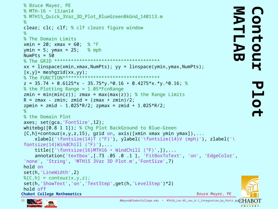
[email protected] • MTH16_Lec-01_sec_6-1_Integration_by_Parts.pptx 25
Bruce Mayer, PE Chabot College Mathematics
Co
nto
ur P
lot M
AT
LA
B
% Bruce Mayer, PE% MTH-16 • 13Jan14% MTH15_Quick_3Var_3D_Plot_BlueGreenBkGnd_140113.m%clear; clc; clf; % clf clears figure window%% The Domain Limitsxmin = 20; xmax = 60; % °Fymin = 5; ymax = 25; % mphNumPts = 50% The GRID **************************************xx = linspace(xmin,xmax,NumPts); yy = linspace(ymin,ymax,NumPts);[x,y]= meshgrid(xx,yy);% The FUNCTION***********************************z = 35.74 + 0.6125*x - 35.75*y.^0.16 + 0.4275*x.*y.^0.16; %% the Plotting Range = 1.05*FcnRangezmin = min(min(z)); zmax = max(max(z)); % the Range LimitsR = zmax - zmin; zmid = (zmax + zmin)/2;zpmin = zmid - 1.025*R/2; zpmax = zmid + 1.025*R/2;% % the Domain Plotaxes; set(gca,'FontSize',12);whitebg([0.8 1 1]); % Chg Plot BackGround to Blue-Green[C,h]=contour(x,y,z,15), grid on, axis([xmin xmax ymin ymax]),... xlabel('\fontsize{14}T (°F)'), ylabel('\fontsize{14}V (mph)'), zlabel('\fontsize{14}WindChill (°F)'),... title(['\fontsize{16}MTH16 • WindChill (°F)',]),... annotation('textbox',[.73 .05 .0 .1 ], 'FitBoxToText', 'on', 'EdgeColor', 'none', 'String', 'MTH15 3Var 3D Plot.m','FontSize',7)hold onset(h,'LineWidth',2)%[C,h] = contour(x,y,z);set(h,'ShowText','on','TextStep',get(h,'LevelStep')*2)hold off

[email protected] • MTH16_Lec-01_sec_6-1_Integration_by_Parts.pptx 26
Bruce Mayer, PE Chabot College Mathematics
WindChill Surface Plotted
2030
4050
60
510
1520
2530
10
20
30
40
50
60
T (°F)
MTH16 • WindChill Function
V (mph)
Win
dC
hill
(°F
)
MTH15 3Var 3D Plot.m
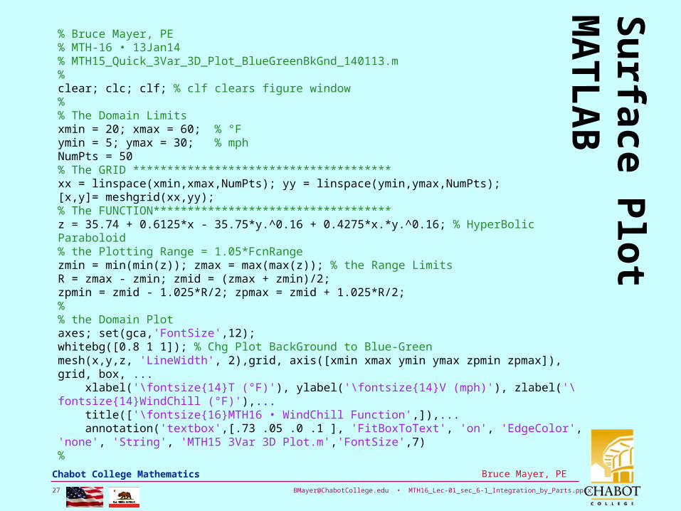
[email protected] • MTH16_Lec-01_sec_6-1_Integration_by_Parts.pptx 27
Bruce Mayer, PE Chabot College Mathematics
Su
rface Plo
t MA
TL
AB
% Bruce Mayer, PE% MTH-16 • 13Jan14% MTH15_Quick_3Var_3D_Plot_BlueGreenBkGnd_140113.m%clear; clc; clf; % clf clears figure window%% The Domain Limitsxmin = 20; xmax = 60; % °Fymin = 5; ymax = 30; % mphNumPts = 50% The GRID **************************************xx = linspace(xmin,xmax,NumPts); yy = linspace(ymin,ymax,NumPts);[x,y]= meshgrid(xx,yy);% The FUNCTION***********************************z = 35.74 + 0.6125*x - 35.75*y.^0.16 + 0.4275*x.*y.^0.16; % HyperBolic Paraboloid % the Plotting Range = 1.05*FcnRangezmin = min(min(z)); zmax = max(max(z)); % the Range LimitsR = zmax - zmin; zmid = (zmax + zmin)/2;zpmin = zmid - 1.025*R/2; zpmax = zmid + 1.025*R/2;% % the Domain Plotaxes; set(gca,'FontSize',12);whitebg([0.8 1 1]); % Chg Plot BackGround to Blue-Greenmesh(x,y,z, 'LineWidth', 2),grid, axis([xmin xmax ymin ymax zpmin zpmax]), grid, box, ... xlabel('\fontsize{14}T (°F)'), ylabel('\fontsize{14}V (mph)'), zlabel('\fontsize{14}WindChill (°F)'),... title(['\fontsize{16}MTH16 • WindChill Function',]),... annotation('textbox',[.73 .05 .0 .1 ], 'FitBoxToText', 'on', 'EdgeColor', 'none', 'String', 'MTH15 3Var 3D Plot.m','FontSize',7)%

[email protected] • MTH16_Lec-01_sec_6-1_Integration_by_Parts.pptx 28
Bruce Mayer, PE Chabot College Mathematics
WindChill Plot by MuPAD
[email protected] • MTH16_Lec-01_sec_6-1_Integration_by_Parts.pptx 29
Bruce Mayer, PE Chabot College Mathematics
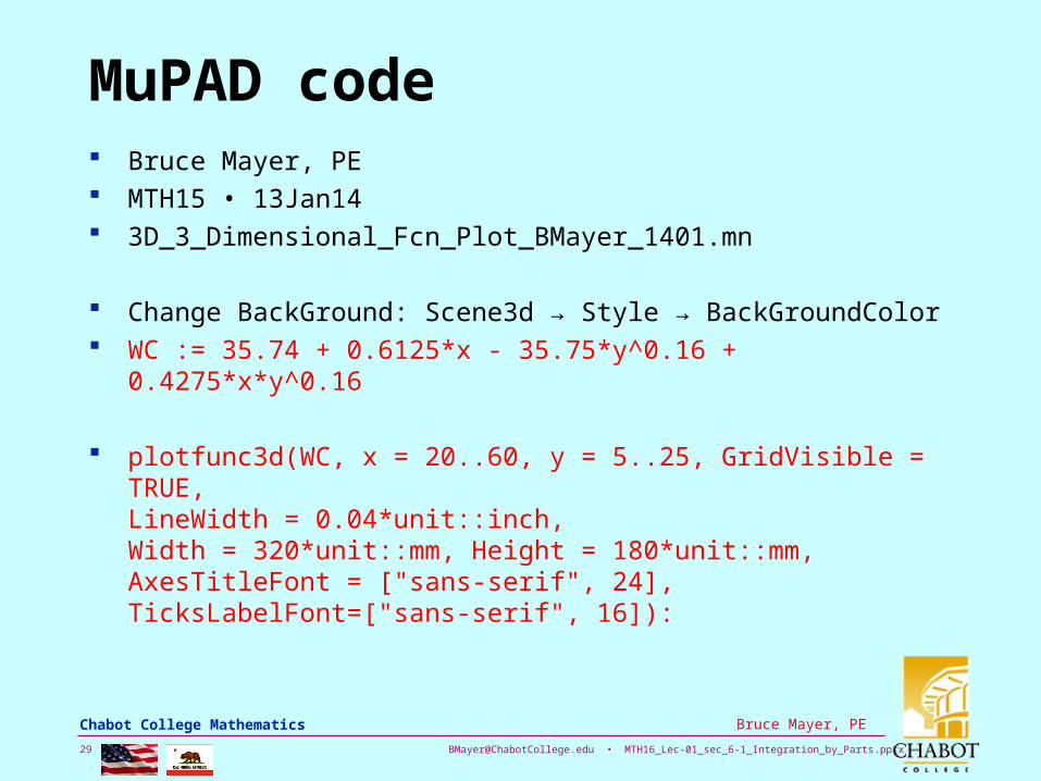
MuPAD code Bruce Mayer, PE MTH15 • 13Jan14 3D_3_Dimensional_Fcn_Plot_BMayer_1401.mn
Change BackGround: Scene3d → Style → BackGroundColor WC := 35.74 + 0.6125*x - 35.75*y^0.16 +
0.4275*x*y^0.16
plotfunc3d(WC, x = 20..60, y = 5..25, GridVisible = TRUE,LineWidth = 0.04*unit::inch, Width = 320*unit::mm, Height = 180*unit::mm,AxesTitleFont = ["sans-serif", 24],TicksLabelFont=["sans-serif", 16]):

[email protected] • MTH16_Lec-01_sec_6-1_Integration_by_Parts.pptx 30
Bruce Mayer, PE Chabot College Mathematics
3D Graphing by Computer
Excel can make Nice 3D Plots for People who do not have MATLAB & MuPAD
To make an Excel Plot, first construct a Basal, or Base Plane
Next Enter “z” formula and calculate Use Insert→Charts→Surface to Create
the Chart And then Fine Tune

[email protected] • MTH16_Lec-01_sec_6-1_Integration_by_Parts.pptx 31
Bruce Mayer, PE Chabot College Mathematics
3D Computer Graphing (Excel)
Basal Plane Detail for
2
2
8.13
yx
ez
-1.5 -1.38 -1.26
-1 -1.17E-03 -2.08E-03 -3.53E-03
-0.92 -1.86E-03 -3.30E-03 -5.60E-03
-0.84 -2.83E-03 -5.04E-03 -8.54E-03
y
x
z =-EXP(-3*(H$7^2/1.8+ $F9^2))

[email protected] • MTH16_Lec-01_sec_6-1_Integration_by_Parts.pptx 32
Bruce Mayer, PE Chabot College Mathematics
Resulting 3D Excel Graph
-1
-0.84
-0.68
-0.52
-0.36-0.2
-0.040.12
0.280.44
0.60.76
0.92
-1.00
-0.90
-0.80
-0.70
-0.60
-0.50
-0.40
-0.30
-0.20
-0.10
0.00
-1.5
-1.3
8-1
.26
-1.1
4-1
.02
-0.9
-0.7
8-0
.66
-0.5
4-0
.42
-0.3
-0.1
8-0
.06
0.06
0.18 0.3
0.42
0.54
0.66
0.78 0.9
1.02
1.14
1.26
1.38 1.5
y
z = (
f(x,
y)
x3D_Surface_Plot_1401.xlsx
3D
_S
urfa
ce_
Plo
t_1
40
1.xlsx

[email protected] • MTH16_Lec-01_sec_6-1_Integration_by_Parts.pptx 33
Bruce Mayer, PE Chabot College Mathematics
-1.5
-1.2
6
-1.0
2
-0.7
8
-0.5
4-0
.3
-0.0
5999
9999
9999
997
0.18
0.42
0.66
0000
0000
0000
1
0.90
0000
0000
0000
11.
141.
38
-1.00
-0.90
-0.80
-0.70
-0.60
-0.50
-0.40
-0.30
-0.20
-0.10
0.00
-1-0.84
-0.68-0.52
-0.36-0.2
-0.040.12
0.280.44
0.60.76
0.92
x
z =
(f(
x,y
)
y3D_Surface_Plot_1401.xlsx

[email protected] • MTH16_Lec-01_sec_6-1_Integration_by_Parts.pptx 34
Bruce Mayer, PE Chabot College Mathematics
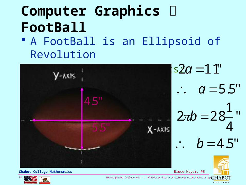
Computer Graphics FootBall
From the National FootBall League RuleBook:• Rule 2 The Ball–Section 1BALL DIMENSIONS
The Ball must be a “Wilson,” hand selected, bearing the signature of the Commissioner of the League, Roger Goodell.
The ball shall be made up of an inflated (12 1/2 to 13 1/2 pounds) urethane bladder enclosed in a pebble grained, leather case (natural tan color) without corrugations of any kind. It shall have the form of a prolate spheroid and the size and weight shall be: long axis, 11 to 11 1/4 inches; long circumference, 28 to 28 ½ inches; short circumference, 21 to 21 1/4 inches; weight, 14 to 15 ounces.
[email protected] • MTH16_Lec-01_sec_6-1_Integration_by_Parts.pptx 35
Bruce Mayer, PE Chabot College Mathematics
Computer Graphics FootBall
A FootBall is an Ellipsoid of Revolution• Using the RuleBook Specs:
"5.5
"5.4"5.5
"112
a
a
"5.4
"4
1282
b
b
[email protected] • MTH16_Lec-01_sec_6-1_Integration_by_Parts.pptx 36
Bruce Mayer, PE Chabot College Mathematics
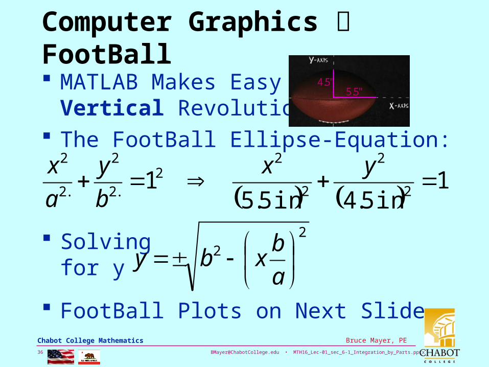
Computer Graphics FootBall
MATLAB Makes Easy Vertical Revolution
The FootBall Ellipse-Equation:
Solvingfor y
FootBall Plots on Next Slide
1
in 5.4in 5.51 2
2
2
22
.2
2
.2
2
yx
b
y
a
x
"5.5"5.4
22
a
bxby

[email protected] • MTH16_Lec-01_sec_6-1_Integration_by_Parts.pptx 37
Bruce Mayer, PE Chabot College Mathematics
Computer Graphics FootBall
0 1 2 3 4
-5
-4
-3
-2
-1
0
1
2
3
4
5
x
y =
f(x)
MTH16 • FootBall
MTH15 Quick Plot BlueGreenBkGnd 130911.m
-5
0
5
-5
0
5
0
2
4
6
8
10
12
x
MTH16 • FootBall
y
z =
f(x,
y)
MTH15 3Var 3D Plot.m
[email protected] • MTH16_Lec-01_sec_6-1_Integration_by_Parts.pptx 38
Bruce Mayer, PE Chabot College Mathematics
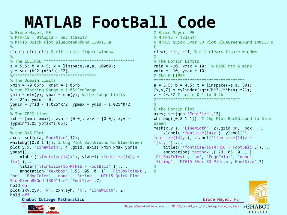
MATLAB FootBall Code% Bruce Mayer, PE% MTH-15 • 01Aug13 • Rev 11Sep13% MTH15_Quick_Plot_BlueGreenBkGnd_130911.m%clear; clc; clf; % clf clears figure window%% The ELLIPSE **************************************a = 5.5; b = 4.5; x = linspace(-a,a, 10000);y = sqrt(b^2-(x*b/a).^2);%***********************************% The Domain Limitsxmin = -0.05*b; xmax = 1.05*b;% the Plotting Range = 1.05*FcnRangeymin = min(y); ymax = max(y); % the Range LimitsR = 2*a; ymid = 0;ypmin = ymid - 1.025*R/2; ypmax = ymid + 1.025*R/2% % The ZERO Lineszxh = [xmin xmax]; zyh = [0 0]; zxv = [0 0]; zyv = [ypmin*1.05 ypmax*1.05];%% the 6x6 Plotaxes; set(gca,'FontSize',12);whitebg([0.8 1 1]); % Chg Plot BackGround to Blue-Greenplot(y,x, 'LineWidth', 4),grid, axis([xmin xmax ypmin ypmax]),... xlabel('\fontsize{14}x'), ylabel('\fontsize{14}y = f(x)'),... title(['\fontsize{16}MTH16 • FootBall',]),... annotation('textbox',[.53 .05 .0 .1], 'FitBoxToText', 'on', 'EdgeColor', 'none', 'String', 'MTH15 Quick Plot BlueGreenBkGnd 130911.m','FontSize',7)hold onplot(zxv,zyv, 'k', zxh,zyh, 'k', 'LineWidth', 2)hold off
% Bruce Mayer, PE% MTH-15 • 13Jan14% MTH15_Quick_3Var_3D_Plot_BlueGreenBkGnd_140113.m%clear; clc; clf; % clf clears figure window%% The Domain Limitsxmin = -10; xmax = 10; % BASE max & min2ymin = -10; ymax = 10;% The ELLIPSE **************************************a = 5.5; b = 4.5; t = linspace(-a,a, 80);[x,y,Z] = cylinder(sqrt(b^2-(t*b/a).^2));z = 2*a*Z % scale 0-1 to 0-2b%***********************************% % the Domain Plotaxes; set(gca,'FontSize',12);whitebg([0.8 1 1]); % Chg Plot BackGround to Blue-Greenmesh(x,y,z, 'LineWidth', 2),grid on, box, ... xlabel('\fontsize{14}x'), ylabel('\fontsize{14}y'), zlabel('\fontsize{14}z = f(x,y)'),... title(['\fontsize{16}MTH16 • FootBall',]),... annotation('textbox',[.73 .05 .0 .1 ], 'FitBoxToText', 'on', 'EdgeColor', 'none', 'String', 'MTH15 3Var 3D Plot.m','FontSize',7)%%

[email protected] • MTH16_Lec-01_sec_6-1_Integration_by_Parts.pptx 39
Bruce Mayer, PE Chabot College Mathematics
WhiteBoard Work
Problems From §7.1• P47 → Skin Surface
Area• P48 → WindMills–Smith-Putnam
WindMillCirca 1941Grandpa's Knob in
Castleton, Vermont
• P49 → Human Energy Expenditure
175 ft

[email protected] • MTH16_Lec-01_sec_6-1_Integration_by_Parts.pptx 40
Bruce Mayer, PE Chabot College Mathematics
All Done for Today
SpiralingFootBall

[email protected] • MTH16_Lec-01_sec_6-1_Integration_by_Parts.pptx 41
Bruce Mayer, PE Chabot College Mathematics
Bruce Mayer, PELicensed Electrical & Mechanical Engineer
Chabot Mathematics
Appendix
–
srsrsr 22
a2 b2
[email protected] • MTH16_Lec-01_sec_6-1_Integration_by_Parts.pptx 42
Bruce Mayer, PE Chabot College Mathematics
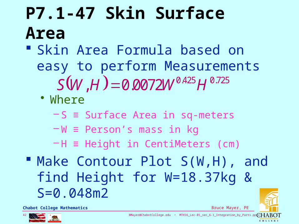
P7.1-47 Skin Surface Area
Skin Area Formula based on easy to perform Measurements
• Where–S ≡ Surface Area in sq-meters–W ≡ Person’s mass in kg–H ≡ Height in CentiMeters (cm)
Make Contour Plot S(W,H), and find Height for W=18.37kg & S=0.048m2
725.0425.00072.0, HWHWS

[email protected] • MTH16_Lec-01_sec_6-1_Integration_by_Parts.pptx 43
Bruce Mayer, PE Chabot College Mathematics
S(15.8kg,87.11cm)
By MuPad• S := 0.0072*(W^0.425)*(H^0.725)
• Sa = subs(S,W=15.83,H=87.11)
– In Sq-Meters

[email protected] • MTH16_Lec-01_sec_6-1_Integration_by_Parts.pptx 44
Bruce Mayer, PE Chabot College Mathematics

[email protected] • MTH16_Lec-01_sec_6-1_Integration_by_Parts.pptx 45
Bruce Mayer, PE Chabot College Mathematics

[email protected] • MTH16_Lec-01_sec_6-1_Integration_by_Parts.pptx 46
Bruce Mayer, PE Chabot College Mathematics

[email protected] • MTH16_Lec-01_sec_6-1_Integration_by_Parts.pptx 47
Bruce Mayer, PE Chabot College Mathematics
Basal Metabolism
The Harris-Benedict Power Eqns for Energy per Day in kgCalories• Human Males
• Human Females
– h ≡ hgt in cm, A ≡ in yrs, w ≡ weight in kg

[email protected] • MTH16_Lec-01_sec_6-1_Integration_by_Parts.pptx 48
Bruce Mayer, PE Chabot College Mathematics
Basal Metabolism
a) Find• Ba := subs(Bm, w=90,h=190,A=22
b) Find• Bb := subs(Bf, w=61,h=170,A=27)d

[email protected] • MTH16_Lec-01_sec_6-1_Integration_by_Parts.pptx 49
Bruce Mayer, PE Chabot College Mathematics
Basal Metabolism
c) Find• Ac := subs(Am, wm=85, hm=193, Bmm=2108)
d) Find• Ad := subs(Af, wf=67, hf=173, Bff=1504)