Embed Size (px)
Citation preview
1
Lucas Parra, CCNY City College of New York
BME I5000: Biomedical Imaging
Lecture 3Intensity Manipulations
Lucas C. Parra, [email protected] some slides inspired by lecture notes of Andreas H. Hilscher at Columbia University.
Blackboard: http://cityonline.ccny.cuny.edu/
2
Lucas Parra, CCNY City College of New York
Schedule
1. Introduction, Spatial Resolution, Intensity Resolution, Noise
2. X-Ray Imaging, Mammography, Angiography, Fluoroscopy
3. Intensity manipulations: Contrast Enhancement, Histogram Equalization
4. Computed Tomography
5. Image Reconstruction, Radon Transform, Filtered Back Projection
6. Positron Emission Tomography
7. Maximum Likelihood Reconstruction
8. Magnetic Resonance Imaging
9. Fourier reconstruction, k-space, frequency and phase encoding
10. Optical imaging, Fluorescence, Microscopy, Confocal Imaging
11. Enhancement: Point Spread Function, Filtering, Sharpening, Wiener filter
12. Segmentation: Thresholding, Matched filter, Morphological operations
13. Pattern Recognition: Feature extraction, PCA, Wavelets
14. Pattern Recognition: Bayesian Inference, Linear classification
3
Lucas Parra, CCNY City College of New York
Contrast
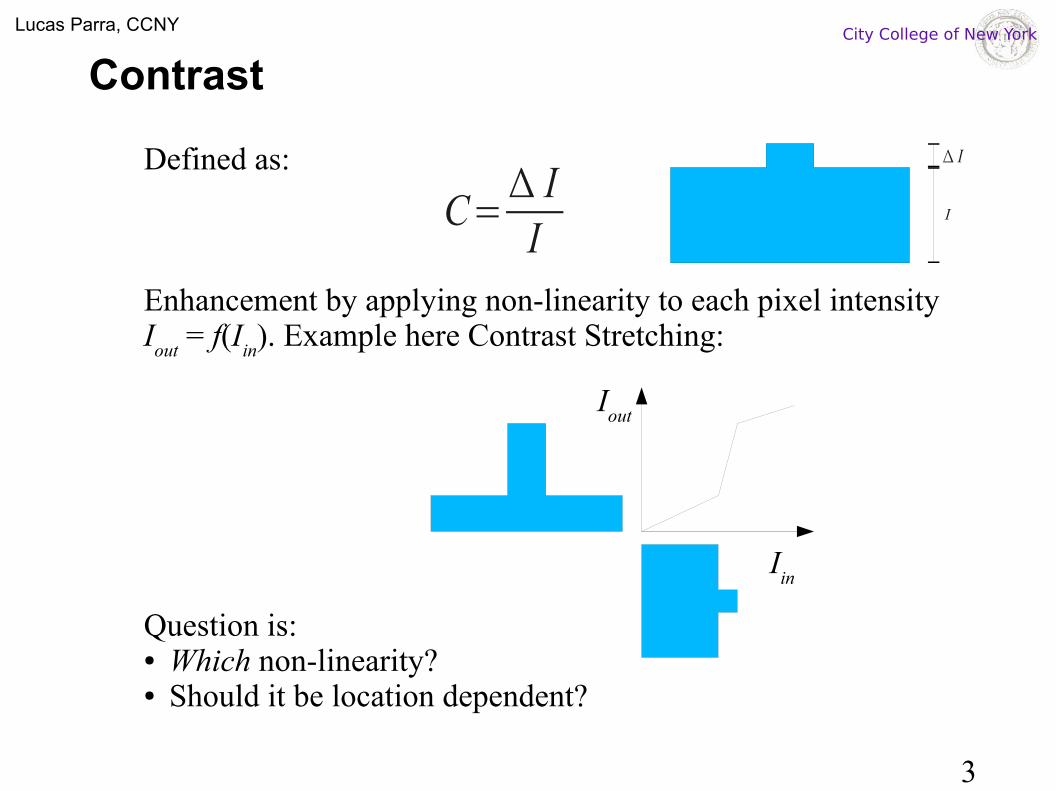
C=Δ I
I
Δ I
I
Defined as:
Enhancement by applying non-linearity to each pixel intensity I
out = f(I
in). Example here Contrast Stretching:
Question is: ● Which non-linearity?● Should it be location dependent?
Iin
Iout
4
Lucas Parra, CCNY City College of New York
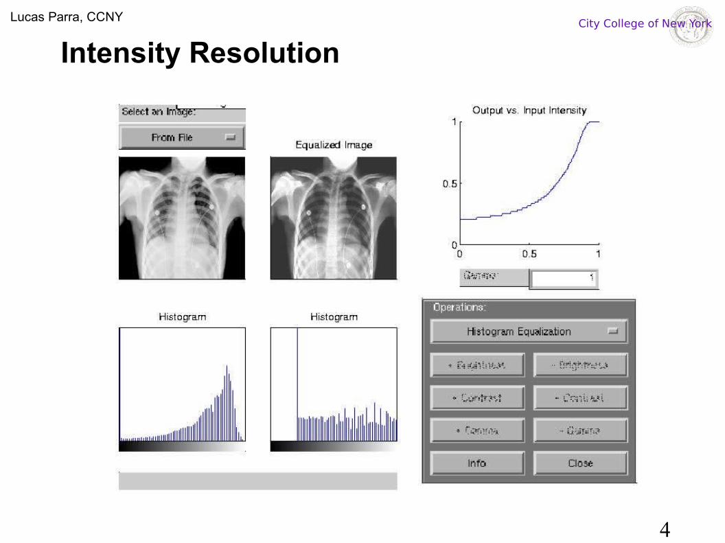
Intensity Resolution
5
Lucas Parra, CCNY City College of New York
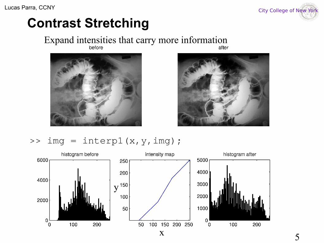
Contrast Stretching
>> img = interp1(x,y,img);
x
y
Expand intensities that carry more information
6
Lucas Parra, CCNY City College of New York
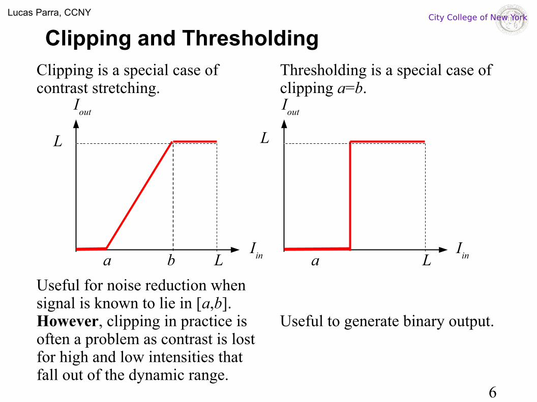
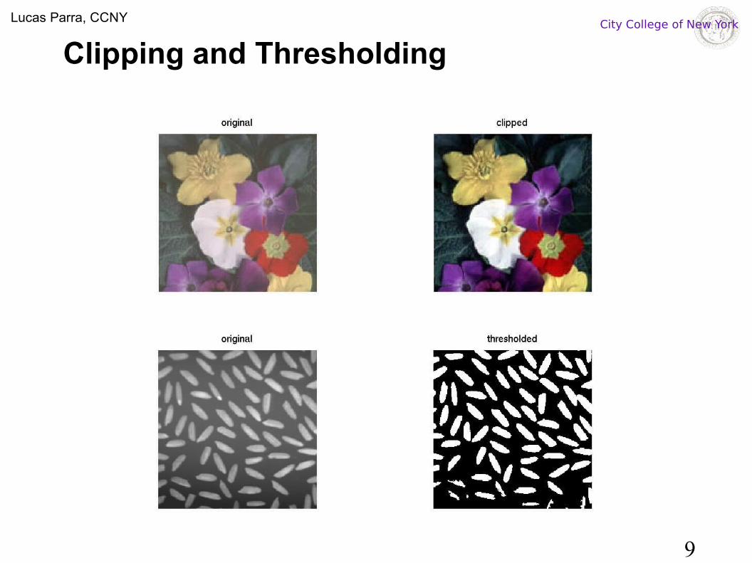
Clipping and ThresholdingClipping is a special case of contrast stretching.
Useful for noise reduction when signal is known to lie in [a,b].However, clipping in practice is often a problem as contrast is lost for high and low intensities that fall out of the dynamic range.
Iin
Iout
a b LI
in
Iout
a L
Thresholding is a special case of clipping a=b.
Useful to generate binary output.
LL
7
Lucas Parra, CCNY City College of New York
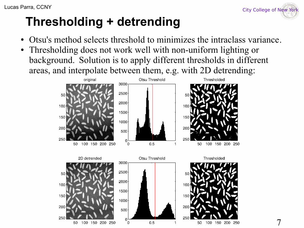
Thresholding + detrending● Otsu's method selects threshold to minimizes the intraclass variance. ● Thresholding does not work well with non-uniform lighting or
background. Solution is to apply different thresholds in different areas, and interpolate between them, e.g. with 2D detrending:
8
Lucas Parra, CCNY City College of New York
Thresholding + detrending
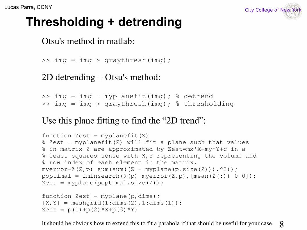
Otsu's method in matlab:
>> img = img > graythresh(img);
2D detrending + Otsu's method:
>> img = img – myplanefit(img); % detrend>> img = img > graythresh(img); % thresholding
Use this plane fitting to find the “2D trend”:
function Zest = myplanefit(Z)% Zest = myplanefit(Z) will fit a plane such that values% in matrix Z are approximated by Zest=mx*X+my*Y+c in a% least squares sense with X,Y representing the column and % row index of each element in the matrix.myerror=@(Z,p) sum(sum((Z - myplane(p,size(Z))).^2));poptimal = fminsearch(@(p) myerror(Z,p),[mean(Z(:)) 0 0]);Zest = myplane(poptimal,size(Z));
function Zest = myplane(p,dims);[X,Y] = meshgrid(1:dims(2),1:dims(1));Zest = p(1)+p(2)*X+p(3)*Y;
It should be obvious how to extend this to fit a parabola if that should be useful for your case.
9
Lucas Parra, CCNY City College of New York
Clipping and Thresholding
10
Lucas Parra, CCNY City College of New York
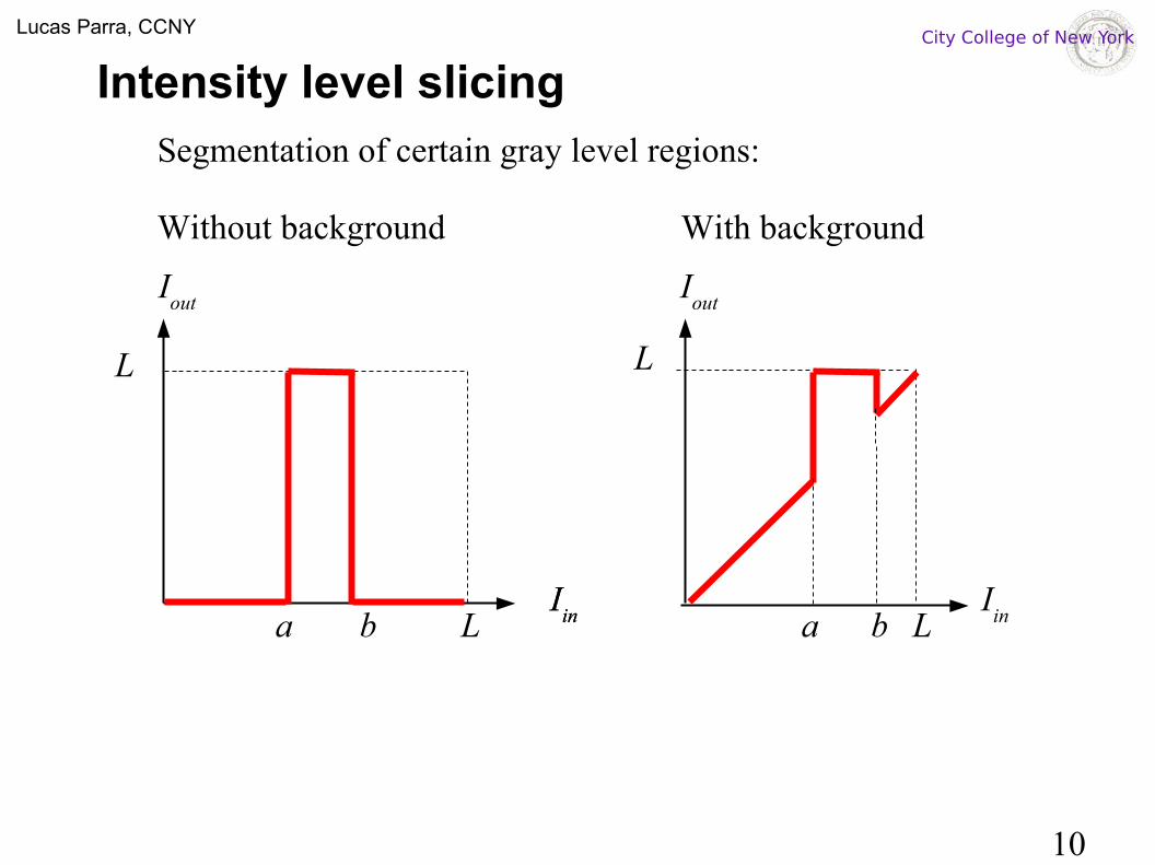
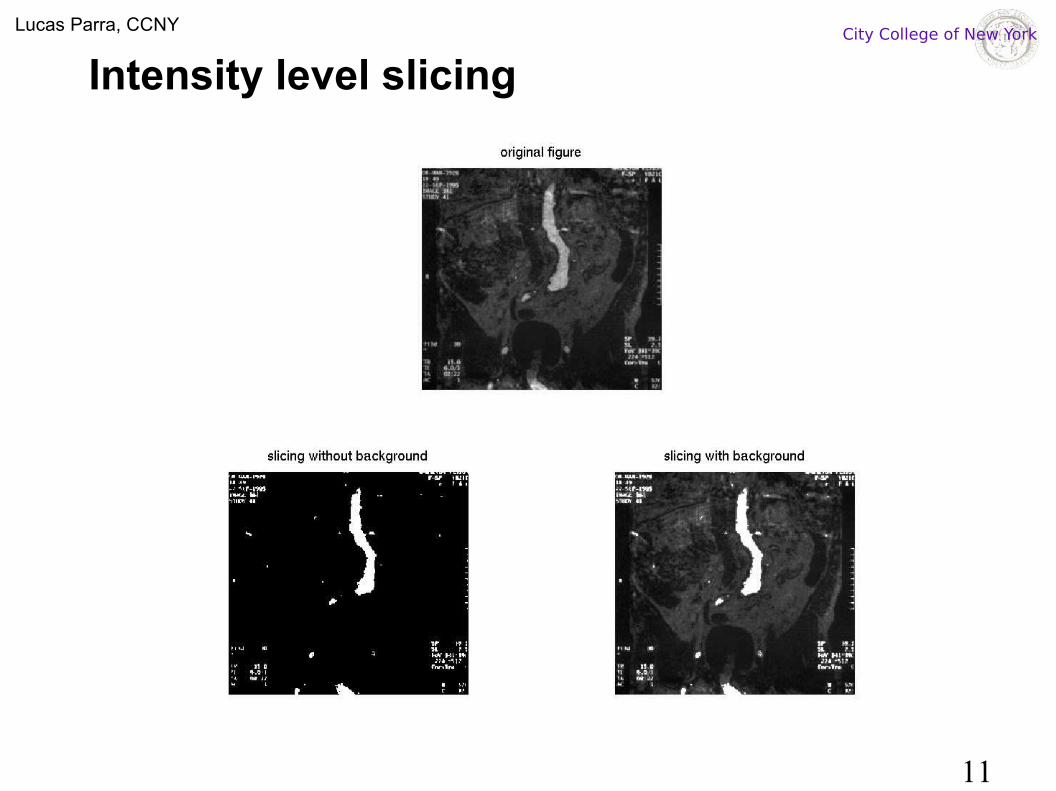
Intensity level slicingSegmentation of certain gray level regions:
Without background With background
Iin
Iout
a b L
L
Iin
Iin
Iout
a L
L
b
11
Lucas Parra, CCNY City College of New York
Intensity level slicing
12
Lucas Parra, CCNY City College of New York
Histogram Equalization
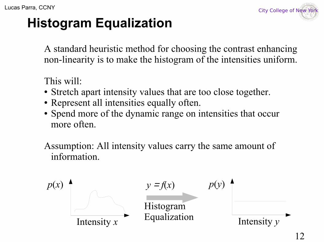
A standard heuristic method for choosing the contrast enhancing non-linearity is to make the histogram of the intensities uniform.
This will: ● Stretch apart intensity values that are too close together. ● Represent all intensities equally often. ● Spend more of the dynamic range on intensities that occur
more often.
Assumption: All intensity values carry the same amount of information.
p(x)
Intensity x
p(y)
Intensity y
y = f(x)
Histogram Equalization
13
Lucas Parra, CCNY City College of New York
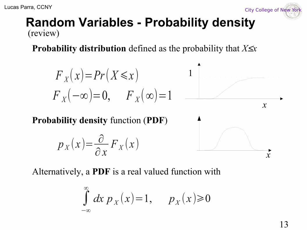
Probability distribution defined as the probability that X≤x
Probability density function (PDF)
Alternatively, a PDF is a real valued function with
Expected valueMoments, Cumulants Poisson, Exponential (Lapace)Normal distributionProduct and convolutions of GaussiansSum of random variablesSample average (law of large numbers)Central limit theorem
(Characteristic function if needed for any of this)
Random Variables - Probability density
F X ( x)=Pr ( X ⩽x )
p X (x )= ∂∂ x
F X (x )x
x
1
F X (−∞)=0, F X (∞)=1
∫−∞
∞
dx p X (x)=1, pX (x )⩾0
(review)
14
Lucas Parra, CCNY City College of New York
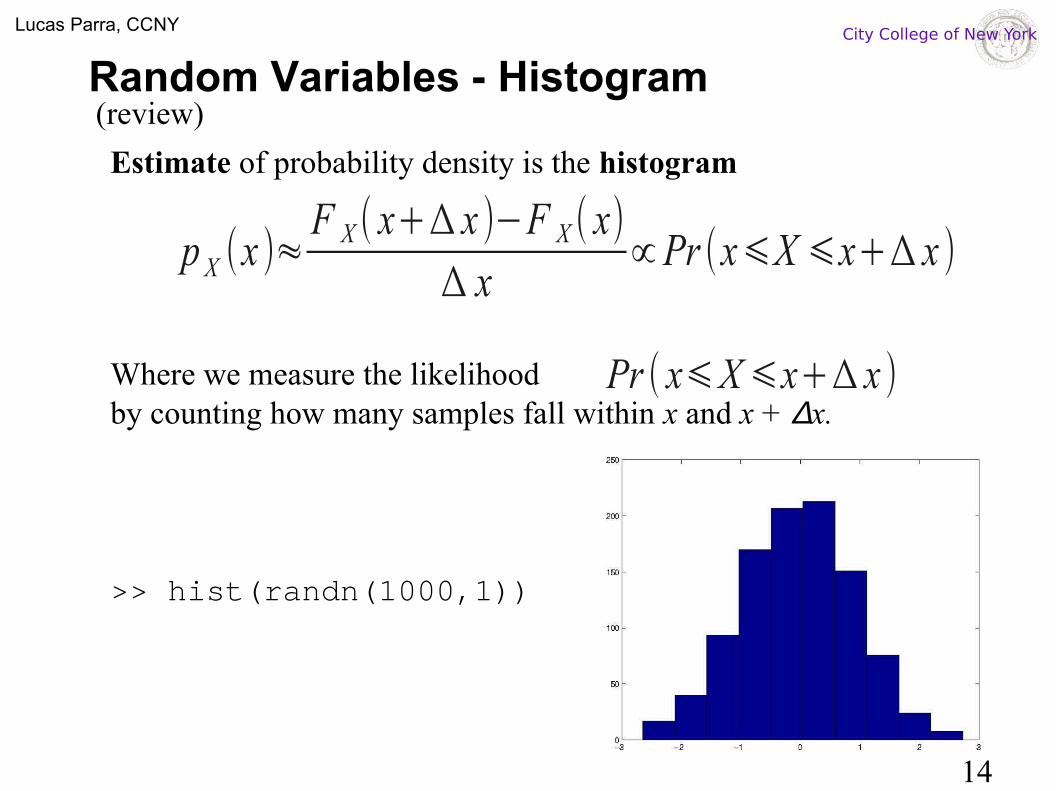
Estimate of probability density is the histogram
Where we measure the likelihoodby counting how many samples fall within x and x + ∆x.
>> hist(randn(1000,1))
Random Variables - Histogram
p X (x )≈F X ( x+Δ x )−F X ( x)
Δ x∝ Pr (x⩽X ⩽x+Δ x )
Pr ( x⩽X ⩽x+Δ x )
(review)
15
Lucas Parra, CCNY City College of New York
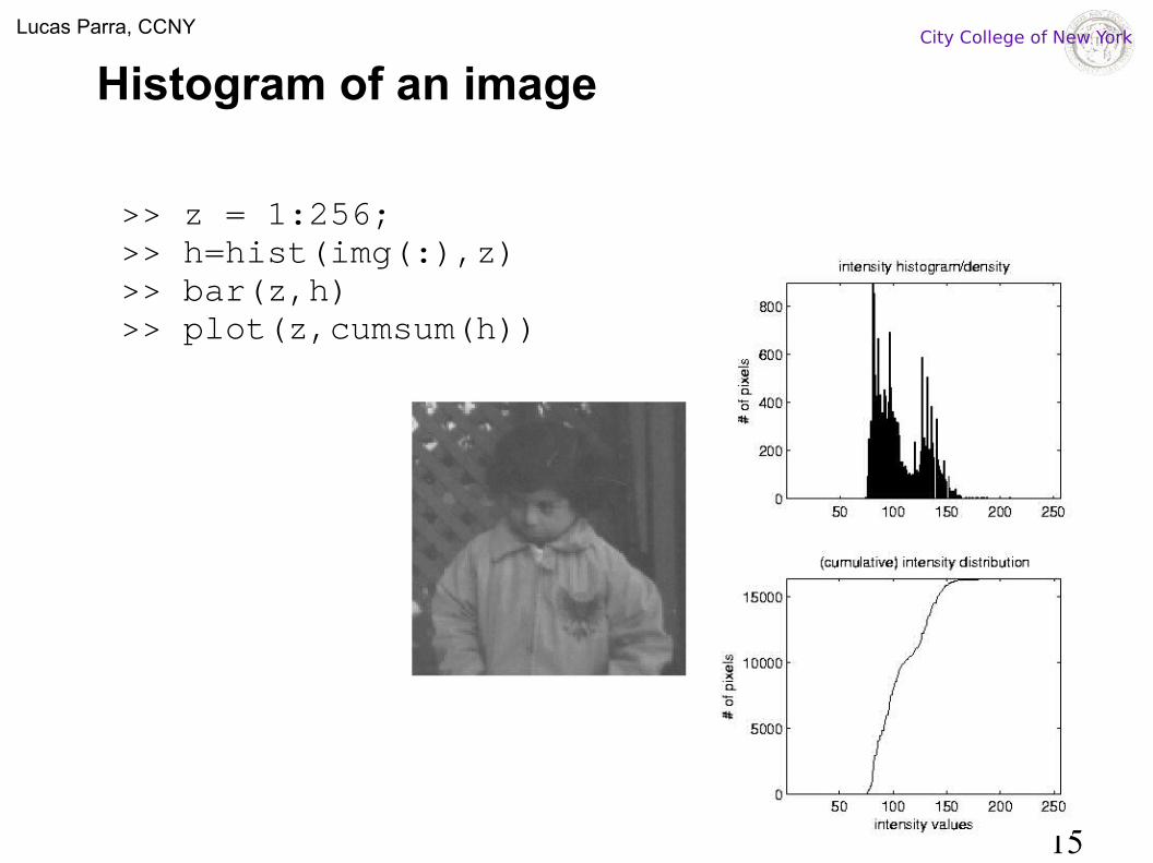
>> z = 1:256;>> h=hist(img(:),z)>> bar(z,h)>> plot(z,cumsum(h))
Histogram of an image
16
Lucas Parra, CCNY City College of New York
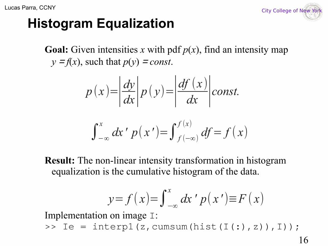
Histogram Equalization
Goal: Given intensities x with pdf p(x), find an intensity map y = f(x), such that p(y) = const.
Result: The non-linear intensity transformation in histogram equalization is the cumulative histogram of the data.
Implementation on image I:>> Ie = interp1(z,cumsum(hist(I(:),z)),I));
y= f ( x)=∫−∞
xdx ' p( x ' )≡F ( x)
p (x )=∣dydx∣p ( y)=∣df (x )
dx ∣const.
∫−∞
xdx ' p( x ' )=∫f (−∞)
f (x)
df = f ( x)
17
Lucas Parra, CCNY City College of New York
Histogram Equalization - Local
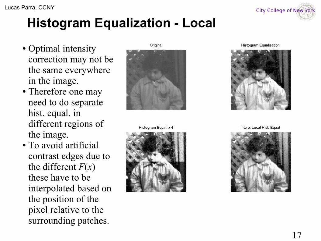
● Optimal intensity correction may not be the same everywhere in the image.
● Therefore one may need to do separate hist. equal. in different regions of the image.
● To avoid artificial contrast edges due to the different F(x) these have to be interpolated based on the position of the pixel relative to the surrounding patches.
18
Lucas Parra, CCNY City College of New York
Histogram Equalization - Local
Demonstration: 1. Implement histogram equalization using the functions
hist(), cumsum(), interp1() 2. Apply histogram equalization separately to 4 quadrants of image (upper
left, lower left, upper right, lower right)3. Use the same 4 histograms and the function interp3() to
implement local histogram equalization.
Assignment 4: Generate examples for image clipping, thresholding, slicing with background, and slicing without background. Find images for which you feel that these techniques are useful. Present them as in slide 7 and 9.
Assignment 4 – alternate: Select and image from your research area (e.g. cell cultures, CT, fMRI, spectroscopy, etc) for which you feel that thresholding would be beneficial (e.g. measure an area, or circumference of an area, or number of areas, etc). Use an automated thresholding routine of your choice and compensate for inhomogeneities if necessary. Discuss your choices in your submission.
19
Lucas Parra, CCNY City College of New York
Contrast vs. Noise
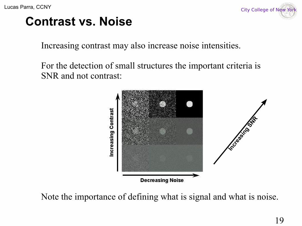
Increasing contrast may also increase noise intensities.
For the detection of small structures the important criteria is SNR and not contrast:
Note the importance of defining what is signal and what is noise.
Incr
easi
ng S
NR
20
Lucas Parra, CCNY City College of New York
Contrast vs. Noise
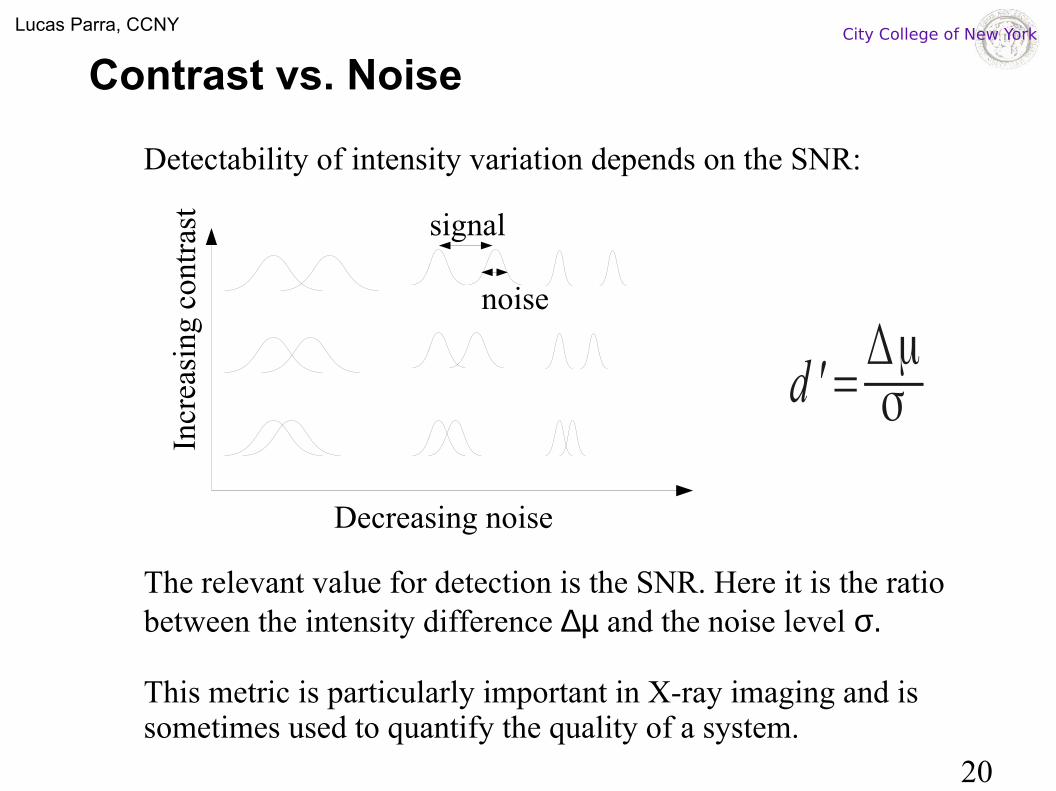
Detectability of intensity variation depends on the SNR:
The relevant value for detection is the SNR. Here it is the ratio between the intensity difference ∆µ and the noise level σ.
This metric is particularly important in X-ray imaging and is sometimes used to quantify the quality of a system.
signal
noise
Decreasing noise
Incr
easi
ng c
ontr
ast
d ' =Δμσ