Embed Size (px)
Citation preview

Draft Revision
BMP COSTS & SAVINGS STUDY
A Guide to Data and Methods for Cost-Effectiveness Analysis of
Urban Water Conservation Best Management Practices
March 2005
Prepared for
The California Urban Water Conservation Council
455 Capitol Mall, Suite 703 Sacramento, CA 95814
916.552.5885
By
A & N Technical Services, Inc.
839 2nd St, Suite 5
Encinitas, CA 92024 760.942.5149
ii
Preface to the Revision The present revision to the Cost and Savings Study has taken place in two parts. This document contains both parts, completed in the first and second year respectively of the revision process. The following sections have been revised—or added to—the Cost and Savings Study.
• A new chapter on Program Cost Accounting has been added (Chapter 3) • Section 1 has been slightly revised to include two new tables—one regarding BMP
requirements and the other summarizing costs and savings. The matrix table has also been revised to reflect the additional conservation devices and activities.
• A new section for each of the following topics o Conservation Pricing o Irrigation Controllers (Residential) o Food Service Equipment o Film Processing (X-Ray)
• A revised section on the following topics: o High Efficiency Washers o Hot Water Circulation on Demand o Universal Metering and Submetering o Large Landscape o Residential Ultra Low Flow Toilets o CII Ultra Low Flow Toilets o Residential Surveys o CII Surveys, Cooling o System Audits and Leak Detection o Residential plumbing retrofits (minor revision)
Other sections of the document remain unchanged.
iii
Acknowledgements This project was supported by and prepared for the California Urban Water Conservation Council. CUWCC signatories that contributed to the original project fund include:
Alameda County Water District City of Santa Monica Contra Costa Water District East Bay Municipal Utility District Kern County Water Agency Los Angeles Department of Water and Power Metropolitan Water District of Southern California San Diego County Water Authority Santa Clara Valley Water District
Funding for the revisions has been provided by the following: United States Bureau of Reclamation
CUWCC and A&N Technical Services appreciate the time and energy contributed by the Project Advisory Committee of the Research and Evaluation Committee: Dick Bennett, East Bay Municipal Utility District Eric Cartwright, Alameda County Water District Mary Lou Cotton, Kern County Water Agency Mary Ann Dickinson, California Urban Water Conservation Council
David Fullerton, National Heritage Institute Michael Hollis, Metropolitan Water District of Southern California
David Mitchell, M.Cubed Susan Munves, City of Santa Monica Tom Panella, Planning and Conservation League Greg Smith, California Department of Water Resources Meena Westford, United States Bureau of Reclamation Additional committee members and contributors to this revision include: Conner Everts, P.O.W.E.R.
John Koeller, Koeller and Co. Bill Maddaus, Maddaus Water Management
Lisa Maddaus, Brown and Caldwell Katie Shulte Joung, California Urban Water Conservation Council
Much of the savings and cost information in this document has been published previously in other sources. Though we are grateful to build on this previous work, the errors that remain are our own.

iv
Contents ACKNOWLEDGEMENTS ........................................................................................................III
CONTENTS................................................................................................................................. IV
1 INTRODUCTION .................................................................................................................. 1
1.1 PURPOSE AND CAVEATS................................................................................................. 1 1.2 DEFINITIONS OF KEY CONCEPTS USED IN THIS REPORT............................................... 3 1.3 DEVICES AND ACTIVITIES POTENTIALLY APPLICABLE TO BMPS ................................... 6 1.4 EXAMPLE OF CBA AND CEA........................................................................................ 12 1.5 KNOWN AREAS WHERE FUTURE RESEARCH IS NEEDED ............................................ 12
2 CONSERVATION DEVICES AND ACTIVITIES: COSTS AND SAVINGS................ 1
2.1 IRRIGATION CONTROLLERS (RESIDENTIAL).................................................................... 2 2.2 GRAYWATER ................................................................................................................... 9 2.3 HIGH EFFICIENCY WASHING MACHINES....................................................................... 13 2.4 HOT WATER RECIRCULATION ON DEMAND (RESIDENTIAL) ........................................ 20 2.5 UNIVERSAL METERING AND MULTI-FAMILY SUBMETERING ......................................... 25 2.6 CONSERVATION PRICING .............................................................................................. 35 2.7 RESIDENTIAL PLUMBING RETROFITS............................................................................ 40 2.8 RESIDENTIAL SURVEYS................................................................................................. 47 2.9 ULTRA LOW FLUSH TOILETS (RESIDENTIAL)................................................................ 54 2.10 CII SURVEYS: COOLING AND INDUSTRIAL PROCESSES............................................... 65 2.11 FILM PROCESSING (X-RAY).......................................................................................... 74 2.12 FOOD SERVICE EQUIPMENT ......................................................................................... 79 2.13 SELF-CLOSING FAUCETS.............................................................................................. 86 2.14 ULTRA LOW FLUSH TOILETS (CII) ................................................................................ 91 2.15 URINALS ........................................................................................................................ 96 2.16 LARGE LANDSCAPE..................................................................................................... 101 2.17 SYSTEM AUDITS AND LEAK DETECTION ..................................................................... 112
3 PROGRAM COST ACCOUNTING ................................................................................... 1
3.1 TEMPLATES TO STRUCTURE COST ACCOUNTING .......................................................... 1 3.2 DISCUSSION .................................................................................................................... 3 3.3 NUMERICAL EXAMPLE ..................................................................................................... 4 3.4 DISCUSSION .................................................................................................................... 7 3.5 CONCLUSION................................................................................................................... 9
APPENDIX A: Example Cost-Benefit and Cost-Effectiveness Calculations
Introduction
California Urban Water Conservation Council 1-1
1 Introduction 1.1 Purpose and Caveats
The California Urban Water Conservation Council (CUWCC) is charged with implementing The Memorandum of Understanding Regarding Urban Water Conservation in California (MOU). To this aim, CUWCC developed and published its “Guidelines to Conduct Cost-Effectiveness Analysis of Urban Water Conservation Best Management Practices,” in 1996, which hereafter is referred to as the “CEA Guidelines”.1 CUWCC’s Measurement and Evaluation Committee commissioned this report to extend the previous efforts at developing methods and data to enact the economic analysis provisions of the MOU.
What this document attempts to do:
• To supplement CUWCC’s existing CEA Guidelines by explicitly linking conservation
program costs and water savings to the MOU’s set of Best Management Practices (BMPs);
• To identify and summarize the best available information about program costs and water savings;
• To assess the reliability and generalizability of information currently available for quantifying and valuing conservation activity and for preparing cost-effectiveness exemption claims; and
• To identify the absence of, and note critical deficiencies in, cost and savings estimates needed to quantify and to gauge the cost-effectiveness of specific BMPs.
What this document does not do:
• Provide or endorse the use of single, uniform estimates of programs costs and water savings. Differences in each agency’s service area characteristics preclude a ‘cookbook’ approach to calculating the costs and the effectiveness of conservation programs.
• Pretend to provide definitive or complete estimates. Indeed, a conscious effort has been made to highlight the limitations of currently available estimates of program costs and water savings.2
• Repeat material already covered in the companion, CEA Guidelines. 1 See “Guidelines to Conduct Cost-Effectiveness Analysis of Urban Water Conservation Best Management Practices,” prepared by A&N Technical Services for CUWCC, September 1996. 2 The Measurement & Evaluation Committee strongly recommends that the CUWCC consider ways of remedying these deficiencies and that the information in this document be reviewed and updated on an annual basis.

Introduction
California Urban Water Conservation Council 1-2
Caveat: Generalizability3
The conservation savings estimates summarized in this document are drawn from a variety of studies conducted using different methods (e.g., engineering estimates developed in laboratory settings versus measuring changes in actual household water use following a ULFT retrofit); at different times (e.g., during versus after a drought episode, or during the earlier versus later stages of market saturation); in different geographic regions; and for different customer groups (e.g. owners versus renters; residential versus non-residential sectors). Careful thought should always be given to factors that may limit the applicability or generalizability of the cost and savings estimates developed by the studies summarized in this document. In some cases, it may be necessary to use service area specific information or professional judgment to adjust the estimates reported in this document to more meaningfully fit the distinctive characteristics and circumstances of different service territories. When making such applications and judgments, one must bear the burden of showing that they are warranted, reasonable and appropriate.
Caveat: Economic Terminology
Often, the cost-effectiveness of conservation is expressed in dollars per unit (for example, $/AF). Also note that conservation activities are often referred to as “cost-effective” if they have dollar valued benefits that exceed costs (e.g., positive net present value, NPV). This mix of usage has led to some confusion regarding the distinction between “cost-effectiveness analysis” and “cost-benefit analysis.” The MOU, for example, defines a BMP as “cost-effective” when the present value of its benefits exceeds the present value of its costs—that is, when NPV is positive. The CEA Guidelines closely follow the original MOU nomenclature. In contrast, this document employs nomenclature intended to more formally, and more properly, distinguish between cost-benefit analysis and cost-effectiveness analysis. We also seek to clarify the distinction with definitions (below) and the example presented in Appendix A.
Caveat: Common Errors in the use of Conservation Savings Estimates
The following list of common errors is important to remember at the outset of an analysis of conservation savings:
• Not accounting for ongoing savings due to natural replacement; • Not identifying whether savings are “net” of other possible causes aside from the
conservation program under consideration; and • Not accounting for the decay in conservation savings, should such decay exist.
3 In addition to the issue of generalizability, studies of conservation savings and costs need to be concerned with threats to reliability and validity. Has random measurement error contributed to incorrect statistical conclusions? Has an event occurred in the test period that could influence the outcome of a study? We urge the careful consideration of such questions when drawing on the results summarized in this document to analyze water savings of BMP conservation practices. This document only begins the discussion of reliability, validity, and generalizability of savings and cost results; future research is needed to address these issues rigorously. See also Hollis, M., A. Bamezai, and D. Pekelney, “The Reliability and Validity of Conservation Measures,” Proceedings of the American Water Works Annual Conference (1998).
Introduction
California Urban Water Conservation Council 1-3
1.2 Definitions of Key Concepts Used in this Report
This section seeks to standardize the language used to discuss and describe conservation BMPs and their analysis. Thereby, we hope to minimize ambiguous communication and to move toward standardized BMP cost-effectiveness reporting:
A conservation device is a piece of equipment or hardware used to conserve water. Low-flow showerheads, ultra-low-flush toilets (ULFTs), and cooling tower controllers are examples of conservation devices.
A conservation activity is an action performed to conserve water. Water audits and surveys, irrigation timer adjustments, leak detection, public service announcements, and school education programs are conservation activities. Some, but not all, conservation activities may involve the installation of conservation devices (for example, residential surveys that include installation of low-flow showerheads).
A conservation program is a means by which devices are installed and activities are performed. Examples of programs include ULFT rebate programs to promote installation of ultra-low-flush toilets and commercial, industrial, and institutional (CII) survey programs to promote more effective adjustment of cooling tower controllers. When considering costs, it is important to address the administrative time and overhead related to the delivery of devices and activities. Likewise, when considering savings, it is important to distinguish between various program delivery mechanisms if these options result in different amounts of water saved.
Important perspectives of analysis include the total society perspective, the supplier perspective, the supplier perspective with cost sharing, and the customer perspective. The total society perspective concerns itself with summing all of the costs and benefits to society. The supplier perspective is concerned with summing the cost and benefits to the supplier, with and without cost sharing with other agencies such as wastewater agencies. Likewise, the customer perspective sums the costs and benefits to customers—both those participating in the program and those not participating. Chapter 1 of the CEA Guidelines describes the perspectives of analysis most central to the MOU’s exemption process, including the total society perspective, the supplier perspective, and the supplier perspective with cost sharing. One of the goals of this document is to assemble data for the supplier and total society perspectives. Perspective of analysis is one of several key factors that influence the estimation of costs and water savings of water conservation programs. Other key factors include the natural replacement rate of conservation devices and the existence of uniform plumbing standards. In what follows, this section defines these factors and describes ways to account for them when analyzing the costs and benefits of BMPs. The benefits of water conservation programs include all of the positive results of program efforts to increase water use efficiency. Benefits are determined first by measuring water savings, which are quantified in physical units (e.g., gpd) by comparing water consumption with and without conservation devices or activities. When conducting cost-benefit analysis, water savings are expressed in dollar terms. The dollar value of water savings is determined by assessing factors such as the avoided costs of water supply and the avoided costs of wastewater treatment. Benefits also include environmental benefits; for an introduction to environmental benefits valuation readers should look to the CEA Guidelines.

Introduction
California Urban Water Conservation Council 1-4
When determining conservation savings, it is important to identify incremental savings
that the program produces—that is, water savings that would not have resulted without the program. Active conservation refers to incremental savings resulting from supplier-assisted conservation programs. Passive conservation refers to water savings resulting from customer actions and activities, which do not involve, or depend on, direct assistance from supplier-assisted conservation programs. The additional increment of active conservation above passive conservation is the savings needed for cost-effectiveness calculations of suppliers’ programs. Consider, for example, the water savings resulting from replacing an older toilet with a new water efficient model. If the replacement would not occur otherwise, but is motivated by a utility-sponsored rebate program, the resulting water savings should be counted as active conservation. But if the customer replaces a broken toilet that needs to be replaced immediately even without the rebate program, the savings should be counted as passive conservation.4 The difference between active and passive savings has a direct bearing on program cost-effectiveness.
Customers who participate in a rebate program, but who would have conserved without
the program, are known as free riders. When assessing program cost-effectiveness, water savings accruing as the result of program participation by free riders should not be credited to the program. In other words, savings from installation of conservation devices by free riders does not represent an additional increment of savings due to the program. For this reason, free riders reduce the cost-effectiveness of utility-sponsored conservation programs.
If there is no water efficiency plumbing code or other standards, then there may be
competing technologies for water consuming appliances such as washing machines, and not all of the competing technologies may be water efficient. In this circumstance, rebate programs may influence not only the customer’s decision of when to replace an appliance (acceleration of savings), but also the decision of what to purchase. Incremental savings are thus the sum of savings due to acceleration of replacement and savings due to the choice of high efficiency technologies (for example, a high efficiency clothes washer).5
Where possible, this report relies on field studies and impact evaluations. The important distinction between field studies and mechanical/engineering estimates is that field studies measure conservation savings in actual use rather than in the lab or on the design table. Field studies are designed to account for variable human behavior, physical performance decay, and other factors encountered in the field.
There are at least three factors intervening between potential savings estimated by engineering/mechanical calculations and actual (or realized) savings measured in field studies:
• Whether the measure is actually implemented--something that can only be known with
certainty through independent, on-site verification; • Validity issues—for example, ANSI sanctioned tests used to measure ULFT flushing
performance may not validly capture the dynamics of in-home use; and • Discretionary behavior—for example, increasing shower time after retrofitting a shower
with a low-flow showerhead.
4 Plumbing codes, city ordinances and discretionary behaviors influenced by a personal “conservation ethic” are the most common factors responsible for passive conservation savings. 5 See Appendix A for a discussion of how accelerated savings affect cost-effectiveness calculations.

Introduction
California Urban Water Conservation Council 1-5
These and other factors can instrumentally affect the amount of water actually saved by
a water efficient device. Where field studies are not available, engineering estimates and assumptions are used. Where neither field nor engineering studies are available, the estimates used in this report are based on professional judgment.
The difference between field studies and mechanical/engineering estimates makes it
important to distinguish between savings potential and actual savings achieved. For example, CII surveys often yield a set of recommendations for conservation devices and activities, which—if fully implemented—would yield a certain level of water savings. But to know if these potential savings are actually realized, it is necessary to know if all of the recommended measures are actually implemented. Failure to properly account for the difference between potential and actual savings can cause program-related water savings to be over-estimated.
Another important factor in correctly estimating conservation savings involves the persistence of savings over time. Savings may decay over time due to lack of maintenance, physical deterioration, and decline in behavioral compliance with conservation activities. As an example of savings decay, large landscape savings often rely on a combination of conservation devices, such as timers, leak repair and sprinkler adjustment, and seasonal timer adjustments. However, if there is a change in landscape contractors, the behavioral component of these measures may be lost without additional training. An example of high persistence is high efficiency washers, which do not require additional maintenance or adjustment over time to continue conserving water.
The amount of potential water savings available to a utility-sponsored conservation
program depends, in part, on program timing and scale. Incremental savings are measured relative to a “no program” alternative—that is, the case where the active conservation program is not implemented. If the background saturation rate of conserving devices is increasing over time due to passive conservation (for example, plumbing code and natural replacement), then active conservation programs will yield diminishing incremental savings. The expected savings from the installation of a conserving device is less as time goes on because on average, there will be fewer and fewer low efficiency devices left in the customer population, and thus a lower chance of the active conservation program resulting in the replacement of a low efficiency device. This same background saturation rate may account for declining savings over time after the device is installed. The important implication is that declining savings from active conservation means declining program cost-effectiveness. Conversely, implementing a program sooner rather than later and increasing the scale of the program may, under certain circumstances, increase cost-effectiveness.
The costs of conservation programs include costs to customers, capital and operation and maintenance expenditures for conservation programs, program administration and implementation costs, and environmental costs. The CEA Guidelines provide categories of costs that should be included for various perspectives of analysis. For example, for the total society perspective, valid cost categories include participant program costs, supplier program costs, and external costs. Program costs can include staff salaries and overhead; vehicle costs; administrative costs to develop, administer, and monitor the program; material costs; and marketing. Program costs and savings may differ according to program design or “delivery mechanism.” For example, CII surveys may be carefully targeted, which increases both their
Introduction
California Urban Water Conservation Council 1-6
costs and presumably their potential for conservation savings compared to less carefully targeted programs.
It is important to identify the incremental costs of the conservation device or activity. For example, when determining the labor costs associated with a conservation program or activity, it is important to include overhead. But only that share of overhead associated hours actually spent working on the conservation activity should be counted. If standard overhead multipliers include cross-subsidies to unrelated functions, they should be corrected to the extent practical.
Cost-effectiveness analysis (CEA) is the comparison of costs of a conservation device or activity, measured in dollars, with its benefits, expressed in physical units (for example, $Costs per AF of savings). Cost-benefit analysis (CBA) is the comparison of costs of a conservation device or activity, measured in dollars, with its benefits, expressed in dollar terms (for example, $Net Benefits = $Benefits - $Costs). The most meaningful measure for purposes of cost-benefit analysis is net present value (i.e., NPV = $PresentValueBenefits – $PresentValueCosts). NPV compares costs and benefits that occur at different periods of time by discounting to determine their present value. The CEA Guidelines discuss these calculations in greater detail. Sometimes it is not clear whether to represent a particular item as a cost or a benefit. For example, from the customer’s perspective, energy savings that result from some conservation devices--such as high efficiency washing machines--imply a reduction in energy costs compared to the no program alternative. Should these energy savings be counted as a reduction in costs or as an increase in benefits? When calculating NPV, it does not matter because, whether characterized as a “negative cost” or a “positive benefit” it still will be part of the NPV calculation. However, for cost-effectiveness calculations (i.e., cost per AF), it needs to be decided whether to subtract the energy savings from the costs of the conservation program. The CEA Guidelines would characterize the energy savings as a benefit, not a cost; for this document, we extend this convention. 1.3 Devices and Activities Potentially Applicable to BMPs
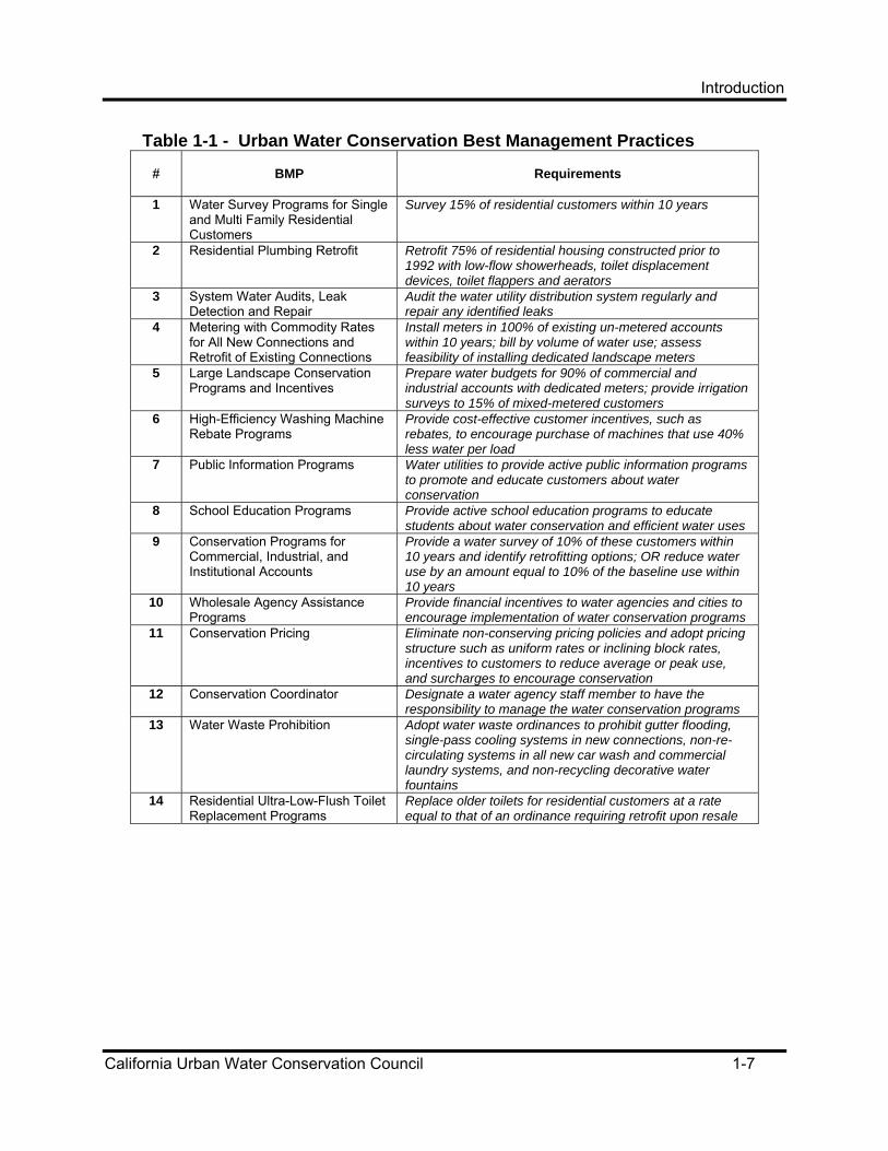
Table 1-1 shows the BMPs contained in the MOU and summarizes the requirements of each one. To fulfill the BMPs, suppliers may put together packages of conservation activities and devices. Table 1-2 shows categories of conservation devices and activities and indicates how they may be related to the BMPs contained in the MOU. Note that some activities and devices relate to more than one BMP. “X” indicates that the device/activity is widely understood to be associated with the BMP or PBMP and “O” indicates potential association.6
6Table 1-1 is not intended to be proscriptive, authoritative, nor limiting to the creativity of future ways to better implement BMPs.
Introduction
California Urban Water Conservation Council 1-7
Table 1-1 - Urban Water Conservation Best Management Practices
#
BMP
Requirements
1 Water Survey Programs for Single and Multi Family Residential Customers
Survey 15% of residential customers within 10 years
2 Residential Plumbing Retrofit Retrofit 75% of residential housing constructed prior to 1992 with low-flow showerheads, toilet displacement devices, toilet flappers and aerators
3 System Water Audits, Leak Detection and Repair
Audit the water utility distribution system regularly and repair any identified leaks
4 Metering with Commodity Rates for All New Connections and Retrofit of Existing Connections
Install meters in 100% of existing un-metered accounts within 10 years; bill by volume of water use; assess feasibility of installing dedicated landscape meters
5 Large Landscape Conservation Programs and Incentives
Prepare water budgets for 90% of commercial and industrial accounts with dedicated meters; provide irrigation surveys to 15% of mixed-metered customers
6 High-Efficiency Washing Machine Rebate Programs
Provide cost-effective customer incentives, such as rebates, to encourage purchase of machines that use 40% less water per load
7 Public Information Programs Water utilities to provide active public information programs to promote and educate customers about water conservation
8 School Education Programs Provide active school education programs to educate students about water conservation and efficient water uses
9 Conservation Programs for Commercial, Industrial, and Institutional Accounts
Provide a water survey of 10% of these customers within 10 years and identify retrofitting options; OR reduce water use by an amount equal to 10% of the baseline use within 10 years
10 Wholesale Agency Assistance Programs
Provide financial incentives to water agencies and cities to encourage implementation of water conservation programs
11 Conservation Pricing Eliminate non-conserving pricing policies and adopt pricing structure such as uniform rates or inclining block rates, incentives to customers to reduce average or peak use, and surcharges to encourage conservation
12 Conservation Coordinator Designate a water agency staff member to have the responsibility to manage the water conservation programs
13 Water Waste Prohibition Adopt water waste ordinances to prohibit gutter flooding, single-pass cooling systems in new connections, non-re-circulating systems in all new car wash and commercial laundry systems, and non-recycling decorative water fountains
14 Residential Ultra-Low-Flush Toilet Replacement Programs
Replace older toilets for residential customers at a rate equal to that of an ordinance requiring retrofit upon resale

Introduction
California Urban Water Conservation Council 1-8
Table 1-2 also illustrates the organization of this report. The report consists of separate
sections that contain savings and cost estimates for each device/activity category for which water savings have been quantified. Within each section there is a range of relevant activities and devices. Note that some of the device/activity categories do not have sections in this report because they do not currently have water savings quantified. Rather than obscure the limitations of currently available information, this report purposely highlights existing deficiencies in an attempt to help the CUWCC identify areas where additional, or improved, information is needed. The report format leaves room to “fill in the blanks” as additional BMP savings are quantified in the future, and as savings and cost estimates are improved. Indeed, it is strongly recommended that the program cost and water savings estimates contained in this report be reviewed and updated annually.
For each conservation device/activity category, the report includes: • Device/Activity Description • Applicable BMPs • Available Water Savings Estimates
- Summary of Savings Estimates - Persistence - Limitations - Confidence in Estimates
• Program and Device/Activity Cost Estimates - Program Costs - Limitations - Confidence in Estimates
• Water Savings Calculation Formula(s) - Calculations - Factors to Consider in Applying the Formula
• Example Calculations • Questions to Ask • Sources
The “Confidence in Estimates” sections designate levels of high, medium, or low
confidence in the reliability and accuracy of specific estimates. These designations are subjective judgments that are meant to indicate the strength of the evidence for savings and cost estimates relative to one another. The “Questions to Ask” sections suggest items to help identify important variables to consider when determining BMP costs and savings.

Introduction
California Urban Water Conservation Council 1-9
Table 1-2 Devices and Activities Potentially Applicable to BMPs*
BMPs
Residen
tial W
ater S
urveys
Residen
tial P
lumbing Retr
ofits
System
Wate
r Audits
, Lea
k Dete
ction
Meterin
g and C
ommodity R
ates
Large L
andsc
ape
High Efficien
cy W
ashing M
achines
Public In
formati
on
School E
ducatio
n
Commercial
, Industr
ial, In
stitutio
nal
Wholesale
Agen
cy A
ssist
ance
**
Conserva
tion Pric
ing
Conserva
tion C
oordinato
r
Water W
aste
Prohibitio
n
Residen
tial U
LFT Rep
lacem
ents
SectorDevice/Activity Category 1 2 3 4 5 6 7 8 9 10 11 12 13 14
Educational Events and Materials X O O X O X X X O
ET Controllers
Graywater Systems O O OHigh EfficiencyWashing Machines O X O O O
Hot Water on Demand Units O O
Metering X O X
Pricing X XResidential Plumbing Retrofit Devices X X
Residential Surveys X X O O
Ultra Low Flush Toilets (Residential) O O O O X
CII Surveys X X
Film Processing (X-Ray) O X
Food Service Appliances O X
Self-Closing Faucets O O X
Ultra Low Flush Toilets (CII) O X
Urinals O X
Large Landscape Devices X X
System Audits and Leak Detection X O
Landscape
Distribution System
Key: X indicates that the device/activity is widely understood to be associated with the BMP or PBMP; O indicates potential association.Notes: * This table is not intended to be proscriptive, authoritative, or limiting to the creativity of future ways to better implement BMPs.** This table does not directly apply to wholesale agencies. Wholesale agencies, under BMP 10 of the MOU, are required to provide financial incentives and/or technical assistance for cost-effective BMPs. Hence, any of the above BMPs/measures may or may not be required to be supported by a wholesale agency depending soley on the cost-effectiveness of that BMP or measure.
Sector
Residential
CII

Introduction
California Urban Water Conservation Council 1-10
Table 1-3 provides an illustrative summary of selected costs and savings with references to the corresponding section of this document.

Introduction
California Urban Water Conservation Council 1-11

Introduction
California Urban Water Conservation Council 1-12
1.4 Example of CBA and CEA
Appendix A provides numerical examples of CBA and CEA that illustrates their
differences and the mechanics of their calculation in a spreadsheet. The examples include, but are not limited to, the following topics described so far:
• Perspectives of analysis; • Presence or absence of plumbing code (low efficiency alternatives); and • Incremental savings and costs.
1.5 Known Areas Where Future Research is Needed
The following is a list of areas that require additional future research:
• Savings decay over time • “Free rider” and “spillover” effects • Discount rates • Natural replacement rates • Device saturation rates • The affects of key program design variables like timing, scale, and targeting • The types and amounts of costs utilities avoid by implementing conservation programs • Expressing program benefits in dollar terms
These areas are addressed in the CEA Guidelines in terms of practical methods for
calculation. Future research in these areas is intended to further develop or add to these methods as well as the cost and savings studies cited in this document.
Conservation Devices and Activities: Costs and Savings
California Urban Water Conservation Council 2-1
2 Conservation Devices and Activities: Costs and Savings
This section contains descriptions for each of the following categories of water conservation devices and activities, grouped by sector:
Residential Sector • ET Controllers (Residential) • Graywater Systems • High Efficiency Washing Machines • Hot Water Demand Units • Metering • Pricing • Residential Plumbing Retrofit Devices • Residential Surveys • Ultra Low Flush Toilets (Residential)
Commercial, Industrial, and Institutional Sector • CII Surveys, Cooling • Film Processing • Food Service • Self-Closing Faucets • Ultra Low Flush Toilets (CII) • Urinals
Landscape Sector • Large Landscape Devices
Distribution System
• System Audits and Leak Detection

Irrigation Controllers
California Urban Water Conservation Council 2-2
2.1 Irrigation Controllers (Residential) 2.1.1 Device/Activity Description This section addresses technologies that automatically adjust irrigation controllers according to the needs of the landscape. In particular, this section covers technologies have been developed to adjust schedules according to real time measures of evapotranspiration (ETo)—or water needs more generally—including temperature, rainfall, soil moisture, and/or sunlight. Historical weather data may also be used in the controller programs. Some of these systems transmit information to the irrigation controller by satellite pager and some include two-way communication via telephone lines (CUWCC 2003). 2.1.2 Applicable BMPs Weather-based irrigation controllers do not fit into any of the BMPs directly. However, in the residential sector they are related to surveys and retrofits in BMPs 1 and 2. The recent technological developments allow ET controllers to serve the single-family sector as well as smaller commercial sites. Thus, these technologies have overlap with small commercial sites not explicitly applicable to BMP 5 Large Landscape. 2.1.3 Available Water Savings Estimates Summary of Individual Studies MWDOC and IRWD (2004) report their most recent in-depth study of their 7 year research program in the Residential Runoff Reduction Study (http://www.mwdoc.com/WaterUse/R3-PDFs/runoff-table-of-contents.htm). The study measured the change in metered water consumption and directly measured urban runoff reduction (in flow volume and water quality). It determined ET controllers reduced household water use on average by 41 gallons per day per single-family household (approximately 10 percent of total household water use); the bulk of the savings occurred in the summer and fall periods. The education-only group of residential customers saved 26 gpd, or about 6 percent of total water use. The savings from this group were more uniform throughout the year. The report provides a discussion of the additional benefit attributable to peak period demand-load reduction. In addition, 15 large landscape sites with dedicated landscape meters were retrofit with ET controllers (ranging in size from 0.14 acres to 1.92 acres) This portion of the study showed average water savings of 545 gpd. Compared to a control group, the retrofit group showed a reduction of 71 percent in dry season runoff. Water quality indicators were highly variable and low statistical power precluded detection of statistically significant differences. Customer acceptance of ET controllers was robust with 72 percent of the participants indicating that they liked the controllers and 70 percent ranking their landscape appearance as good to excellent. IRWD (2001), the “ET Controller Study,” tested a system of controllers that were automatically adjusted using a broadcast signal based on weather conditions. The test group was compared to both a control group without intervention and a group that received postcards with ET information but no automatic controller adjustments. The controllers fitted to the test homes

Irrigation Controllers
California Urban Water Conservation Council 2-3
were all pre-programmed with the same irrigation schedule, which was then modified each week by the broadcast signal. Total household consumption was estimated to decline 7 percent in the post-retrofit year—roughly a 16 percent reduction in outdoor consumption--controlling for weather. This translates into a reduction of 37 gallons per household per day. The author cautions the reader against simplistically applying these savings results to other customers as the program was voluntary and evidence was presented to indicate the study group conservation potential was less than for average customers who had similar initial water consumption. Aqua Conserve (2002) reports that ET controllers adjusted with historical data and temperature sensors successfully conserved water for high-volume residential customers in Colorado and California. Total outdoor water savings were 21 percent in Denver, with an average savings per participant of 21.47 percent. (A symmetric distribution of savings was reported for Denver.) For the City of Sonoma, total outdoor savings were 23 percent, with an average savings per participant of 7.37 percent. (A skewed distribution of water savings was reported for Sonoma.) Valley of the Moon Water District reported 28 percent total savings with an average savings per participant of 25.1 percent. (A symmetric distribution of water savings was reported for Valley of the Moon.) Savings were calculated as post-intervention consumption relative to five-year historical consumption. A control group was used to control for test-year weather. Aquacraft (2003) reports that of the 10 sites included in their study, savings averaged 26,000 gallons per year per site; savings from the 5 largest-saving sites were 68,000 gallons per site. As a group, water application by the controllers was 94 percent of ETo, or 28 inches of water. The sites were a combination of volunteer sites and those with high volume water use; all were residential except for one commercial site. Bamezai (1996) reports savings in a study that considered the effects of connecting multiple meters to a central irrigation controller that controls watering based on ET for each meter. Controlling for climate and landscape size, the average savings per meter at the site was 34 percent. Most of the savings were achieved on sloped areas with diverse plant materials. Persistence Bamezai (2001) reports the results of an analysis of savings in the second year following the retrofit with ET controllers as described in IRWD (2001). Water savings for the entire household was 8.2 percent in the second post-retrofit year, compared to 7.2 percent in the first year. Since these sites were not separately metered, an approximation was used to estimate savings attributed to outdoor use and the ET controller program. Using this approximation, the outdoor savings was 18 percent. DeOreo (1998) reports the results of a study of soil moisture sensors that work in conjunction with conventional irrigation timers to stop watering during rain and whenever soil moisture is otherwise adequate. The study reports that after five years, the sensors “successfully match irrigation applications to requirements with the seasonal applications” … “ranging from 52% to 124% of the theoretical, and the average equaling 76 percent.” The wide range is because the controllers were set to maximum in this test.

Irrigation Controllers
California Urban Water Conservation Council 2-4
Limitations
• For ET controllers to be fully effective, the existing irrigation system must be operated and maintained properly.
• Some studies had to approximate the outdoor water consumption because target sites did not meter landscape use separately.
• The studies more frequently selected large volume customers and volunteers. Care should be taken in generalizing these results as large customers tend to generate large absolute savings figures (not necessarily larger percent savings, however) and volunteers tend to be relatively more receptive to conservation than average.
Confidence in Estimates
Medium. 2.1.4 Program and Device/Activity Cost Estimates Program Costs Participant program costs may include:
• Cost to purchase, install, operate, and maintain the system. Some systems have monthly fees.
Supplier program costs may include:
• Cost to purchase, install, operate, and maintain if supplier shares costs • Administration • Contractors • Marketing
IRWD (2001) states that ET controllers are expected to cost $100 per unit to purchase and $75 to install. The installations were all with a standard set of settings. The monthly signal fee is $4 and the expected life is 10-15 years. Aquacraft (2003) reports that installations of the ET controllers took between 2.25 and 4 hours per site. The installation process included detailed hydro zone measurement and setting the ET controller accordingly. Some sites included moisture sensors. DeOreo (1998) reports—with regard to soil moisture sensors—that the total costs “for repairs and replacements” were $270 (original installation costs not reported). The estimated budget for average annual repairs and replacement was estimated to be $12 per controller. Limitations
• Cost of equipment may depend on volume purchase and installation contracts. • Program design is particularly important to estimating costs because the same

Irrigation Controllers
California Urban Water Conservation Council 2-5
equipment can be used in conjunction with either simple or elaborate tailoring to the particular site or varying levels of outreach and support over time.
Confidence in Estimates Medium-High. 2.1.5 Water Savings Calculation Formula(s) Calculations Estimating prospective savings from a landscape program that utilizes ET controllers involves a comparison of the expected consumption without the controller program to the expected consumption with the program.
Savings = Water_Use_Without_Program - Water_Use_With_Program Expected water use without the program can be projected using historical data. Whitcomb (1994) and A&N Technical Services (1997) present ways of determining weather-normalized consumption. The following water budget equation appears in CUWCC’s BMP 5 Handbook (Whitcomb, J., G. Kah, and W. Willig 1999 as reproduced from Walker, Kah, and Lehmkuhl 1995):
Water_Use_Budget = Irrigated_Area x Adjustment_Factor x Conversion_Factor x (( ETo x KL ) – Effective_Rainfall ) x ( 1 / Irrigation_Efficiency )
where:
• Water_Use_Budget is applied water use requirement for hydro zone during billing period. Overall site water use budget is obtained by summing over all hydro zones.
• Irrigated_Area is landscape area irrigated in hydro zone (typically measured in square feet)
• Adjustment_Factor is scalar between 1.0 and 0.0 determining the allowable stress on the plant material.
• Conversion_Factor is the number converting measurement units into consistent terms. • ETo is reference evapotranspiration for the billing period. ETo is a measure of the
weather’s effect on the need for water by plants. • KL is the coefficient relating a specific plant type’s water requirements to reference ETo. • Effective_Rainfall is the depth of rain effective in offsetting ETo during a billing period. • Irrigation_Efficiency is a factor between 1.0 and 0.0 measuring the efficiency of irrigation
system. Factors to Consider in Applying the Formula
• These figures do not fully reflect behavior that may impact actual savings. For example, maintaining the irrigation equipment in good condition is important to achieve savings.

Irrigation Controllers
California Urban Water Conservation Council 2-6
• The formula is a general budget formula. To be most accurate, consider the specific capabilities of the ET controller under consideration. The controllers do not use the same variables and calculation methods.
• The historical use figures need to be commensurate with the water budget to calculate savings. Thus, one needs to determine outdoor use historically to use in the savings calculations.
• For prospective policy analysis, the water budget can serve as a projection of use if one assumes that the system applies water just in accord with the calculated budget.
• This calculation method above is for one month (or billing period) only; it should be repeated for each month (or billing period) of the year.
• ETo can be expressed in different units. In this example Normal Year ETo, is expressed in terms of monthly (or billing period) totals. More or less detailed calculations can be made with the formula (e.g., daily or yearly).
2.1.6 Example Calculation Tables 1 and 2 show the calculation of a monthly water budget and savings for a sample landscape site with three hydro zones. The three hydro zones are distinguished by plant type, which is indicated in the budget formula by the plant factor (Ash 1998). ETo is expressed in terms of normal year ETo as a monthly total, assuming there is monthly billing with which to compare historical use.
2.1.7 Questions to Ask
• What is the program design that goes along with the ET controller? For example, is there a detailed hydro zone measurement and review, or a simple set of adjustments to the controller?
• How much of the savings can you get with a less costly version of the same program? • What are the life cycle costs including installation, ongoing fees, and maintenance, etc. • How well does the local weather station fit a particular microclimate?
Hydrozone
Irrigated Area
(sq.ft.)Adjustment
FactorConversion
Factor
ETo (inches/ month)
Plant Factor KL
Effective Rainfall (inches)
Irrigation Efficiency
Water Budget
(ccf)Warm Season Turf 1,000 1.0 0.000833 3 1.00 1.0 0.63 2.64 Shrubs 500 1.0 0.000833 3 0.60 1.0 0.63 0.53 Natives 500 1.0 0.000833 3 0.40 1.0 0.63 0.13 Total 2,000 3.31
Table 1 - Water Budget (One Month Billing Period)
Historical Weather Adjusted Outdoor
Use (ccf)
Water Budget
(ccf)Savings
(ccf)10.0 3.3 6.7
Table 2 - Savings from ET Controller

Irrigation Controllers
California Urban Water Conservation Council 2-7
2.1.8 Sources A&N Technical Services (2004), “Residential Runoff Reduction Study, Appendix C: Statistical Analysis of Water Savings,” prepared for the Municipal Water District of Orange County and the Irvine Ranch Water District, July. A&N Technical Services (2004), “Residential Runoff Reduction Study, Appendix D: Statistical Analysis of Urban Runoff Reduction,” prepared for the Municipal Water District of Orange County and the Irvine Ranch Water District, July. A&N Technical Services (1997), “Landscape Water Conservation Programs: Evaluation of Water Budget Based Rate Structures,” prepared for the Metropolitan Water District of Southern California, September. Aqua Conserve (2002), “Residential Landscape Irrigation Study using Aqua ET Controllers,” Information from the CUWCC ET and Weather-Based Irrigation Controllers Workshop, March 2003. URL: http://www.cuwcc.org/et_controllers. Aquacraft (Undated, Downloaded 2003), “Performance Evaluation of WeatherTRAK Irrigation Controllers in Colorado.” URL: www.aquacraft.com. Ash, T. (1998), “Landscape Management for Water Savings: How to Profit from a Water Efficient Future,” Municipal Water District of Orange County. Ash, T. (2002), “Using ET Controller Technology to Reduce Demand and Urban Water Run-Off: Summary of the Technology, Water Savings Potential & Agency Programs,” American Water Works Association Water Sources Conference Proceedings. Bamezai, A. (1996), “Do Centrally Controlled Irrigation Systems Use Less Water? The Aliso Viejo Experience,” prepared for the Metropolitan Water District of Southern California, October. Bamezai, A. (2001), “ET Controller Savings Through the Second Post-Retrofit Year: A Brief Update,” prepared for the Irvine Ranch Water District, April. CUWCC 2003, “ET and Weather-Based Irrigation Controllers Workshop: Product Information,” California Urban Water Conservation Council, March. URL: http://www.cuwcc.org/et_controllers.lasso. DeOreo, W.B., et al. (Undated, Approximately 1998), “Soil Moisture Sensors: Are They a Neglected Tool?” IRWD (2001), “Residential Weather-Based Irrigation Scheduling: Evidence from the Irvine “ET Controller” Study,” Irvine Ranch Water District, the Municipal Water District of Orange County, and the Metropolitan Water District of Southern California, June. MWDOC and IRWD (2004), “The Residential Runoff Reduction Study,” Irvine Ranch Water District, the Municipal Water District of Orange County, July.

Irrigation Controllers
California Urban Water Conservation Council 2-8
Walker, W., G. Kah, and M. Lehmkuhl (1995), “Landscape Water Management: Auditing,” Irrigation Training Research Center, California Polytechnic State University, San Luis Obispo. Whitcomb, J. (1994), Contra Costa Water District, “Weather Normalized Evaluation,” August. Whitcomb, J., G. Kah, and W. Willig (1999), “BMP 5 Handbook: A Guide to Implementing Large Landscape Conservation Programs as Specified in Best Management Practice 5,” California Urban Water Conservation Council, April.

Graywater
California Urban Water Conservation Council 2-9
2.2 Graywater 2.2.1 Device/Activity Description Developed pursuant to the Graywater Systems for Single Family Residences Act of 1992 (AB 3518), the State of California now has graywater system standards in the State Plumbing Code (DWR 1994). "Graywater is untreated household waste water which has not come into contact with toilet waste." Graywater, "Includes: used water from bathtubs, showers, bathroom wash basins, and water from clothes washing machines and laundry tubs." Graywater, "Does not include: waste water from kitchen sinks, dishwashers, or laundry water from soiled diapers." (California Graywater Standards; Title 24, Part 5 of the California Administrative Code). A typical graywater system includes a plumbing system, a surge tank, a filter, a pump and an irrigation system (DWR 1994). 2.2.2 Applicable BMPs Although graywater is not mentioned in BMP 1 – Residential Water Surveys, other means of conserving landscape irrigation water are included. Graywater recommendations or evaluations could be included as part of the residential surveys; however, the BMP does not have provision for gaining credit towards BMP compliance for doing so. It does not appear that graywater could be used toward compliance with BMP 2. 2.2.3 Available Water Savings Estimates Summary of Individual Studies Whitney et al. (1999) estimate the savings from a graywater system to be 446,200 gallons over a 15-year life span. The per capital annual average discharge to the landscape site was 20.4 gallons per day. The California Department of Water Resources Graywater Guide (1994) estimates daily graywater flows for each occupant in a single-family residence. Graywater flow per day per occupant is the sum of flow from showers, bathtubs, washbasins, and clothes washers. Water savings is estimated as the amount of graywater flow that displaces landscape water use that would occur otherwise. A direct method of estimating savings per household in a specific service area is to multiply graywater flow per person by the average number of persons per household in the agency service area. Presumably graywater displaces fresh irrigation water only for the part of the year that landscape is irrigated. Note that usable yield depends on gray water storage capacity and the irrigation requirements at the site, which under current health codes, can be met using graywater.

Graywater
California Urban Water Conservation Council 2-10
Persistence A study that considers the persistence of savings from household graywater systems has not yet been found. Limitations Savings estimates are situation specific and need to account for slope of landscape, vegetation, climate, level of maintenance and other factors. Confidence in Estimates Medium-Low. Future efforts should include empirical measurement of water savings considering behavior (e.g., maintenance), the presence of other low flow devices (e.g., low flow showerheads, faucet aerators, and washing machines), and persistence of savings. Savings estimates may be confounded if wastewater were to be recycled (potential overestimate) or if water percolates to the groundwater basin rather than lost to the sewer (potential underestimate). 2.2.4 Program and Device/Activity Cost Estimates Program Costs Whitney et al. (1999) estimate the costs of equipment and installation for a graywater system fulfilling all legal requirements. Capital costs are estimated to be $5,400 per site, including $1,250 for equipment and $4,150 for labor. Over a 15-year life span, the cost of energy for the pump is estimated to be $100, and backwash water cost is $20. DWR’s Graywater Guide (1994) also estimates the equipment costs of installing a typical graywater system. The costs depend on whether the system uses drip or leach field design. Table 1 summarizes these costs, without labor.
Plumbing Parts 121.00$ Tank Parts 233.00$ Pump 150.00$ Drip Parts (or) 253.00$ Leachfield Parts 230.00$ Total Drip 757.00$ Total Leachfield 734.00$
Table 1 - Equipment Costs of Typical Graywater System ($1994)
Source: DWR Graywater Guide

Graywater
California Urban Water Conservation Council 2-11
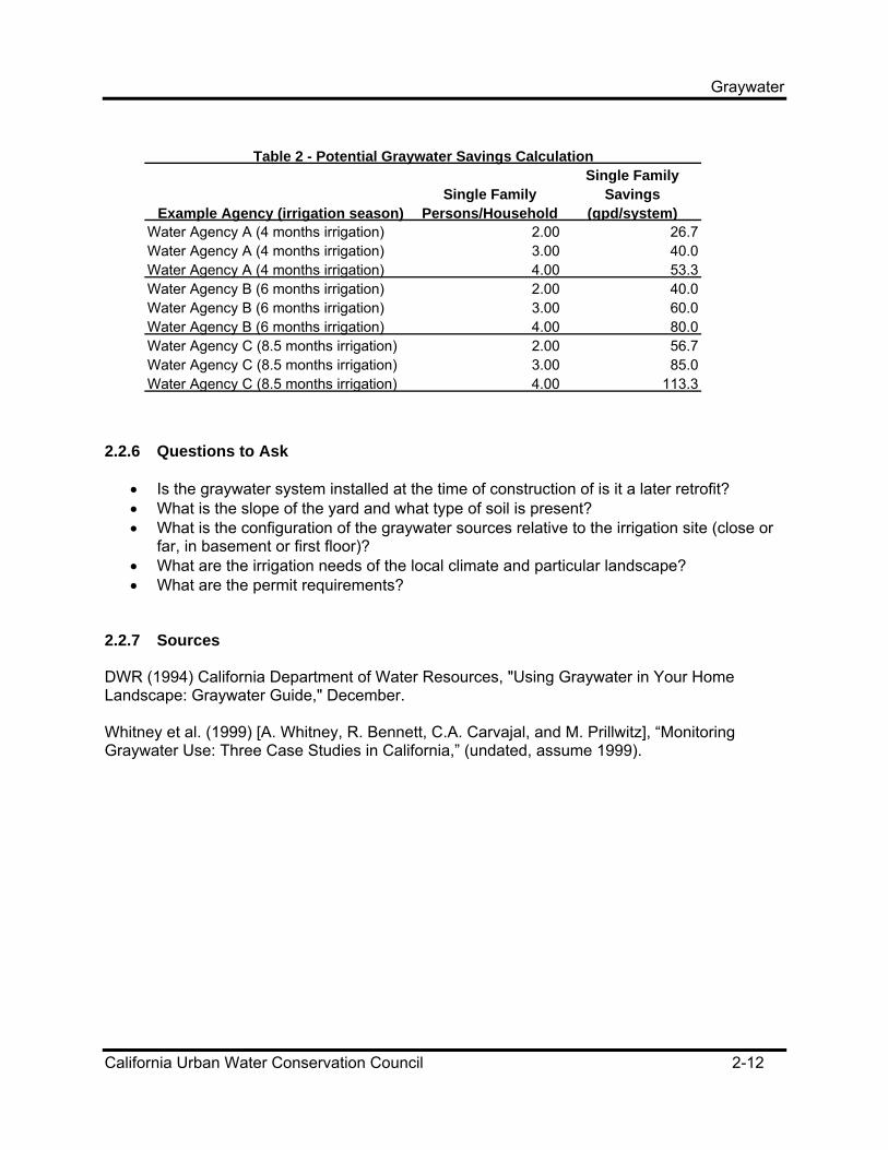
Limitations Often it is complex to get legal permits for graywater systems. Costs depend greatly on the housing construction—whether it is slab foundation, whether it is two story, and/or whether it is new or retrofit construction. Confidence in Estimates Medium-Low. Better cost data is also needed to account for differences in housing construction types (slab foundation, two story, retrofit, etc.). 2.2.5 Water Savings Calculation Formula(s) Calculations The potential graywater savings is calculated by multiplying persons per household times graywater flow per person per day times the percent of irrigation that is saved. Note that the graywater per person per day includes a clothes washer; this figure would be less at sites without clothes washers. S = PPH * Graywater_PPH_Day * Percent_Irrigation_Saved where:
• S is Savings (gpd per household system) • PPH is persons per household • Graywater_PPH_Day is the sum of: (1) showers, bathtubs and washbasins 25 gal. per
day/occupant (DWR 1994) and (2) clothes washers 15 gal. per day/occupant (DWR 1994)
• Percent_Irrigation_Saved is the percent of irrigation days saved (depends on the service area; suggested range of 4 to 8.5 months per year irrigation saved in the example)
Factors to Consider in Applying the Formula Savings estimates should account for site characteristics. Example Calculation The following assumptions were used in the sample calculations:
• Graywater_PPH_Day is the sum of: (1) showers, bathtubs and washbasins 25 gal. per day/occupant (DWR 1994) and (2) clothes washers 15 gal. per day/occupant (DWR 1994)
• Percent_Irrigation_Saved is the suggested range of 4 to 8.5 months per year irrigation Table 2 summarizes estimates for three hypothetical agencies in three climate zones in California, each with a different number of irrigation days that are potentially replaced with graywater.
Graywater
California Urban Water Conservation Council 2-12
2.2.6 Questions to Ask
• Is the graywater system installed at the time of construction of is it a later retrofit? • What is the slope of the yard and what type of soil is present? • What is the configuration of the graywater sources relative to the irrigation site (close or
far, in basement or first floor)? • What are the irrigation needs of the local climate and particular landscape? • What are the permit requirements?
2.2.7 Sources DWR (1994) California Department of Water Resources, "Using Graywater in Your Home Landscape: Graywater Guide," December. Whitney et al. (1999) [A. Whitney, R. Bennett, C.A. Carvajal, and M. Prillwitz], “Monitoring Graywater Use: Three Case Studies in California,” (undated, assume 1999).
Table 2 - Potential Graywater Savings Calculation
Example Agency (irrigation season)Single Family
Persons/Household
Single Family Savings
(gpd/system)Water Agency A (4 months irrigation) 2.00 26.7Water Agency A (4 months irrigation) 3.00 40.0Water Agency A (4 months irrigation) 4.00 53.3Water Agency B (6 months irrigation) 2.00 40.0Water Agency B (6 months irrigation) 3.00 60.0Water Agency B (6 months irrigation) 4.00 80.0Water Agency C (8.5 months irrigation) 2.00 56.7Water Agency C (8.5 months irrigation) 3.00 85.0Water Agency C (8.5 months irrigation) 4.00 113.3

High Efficiency Washing Machines
California Urban Water Conservation Council 2-13
2.3 High Efficiency Washing Machines 2.3.1 Device/Activity Description High efficiency washing machines are those designed to save energy and water. 2.3.2 Applicable BMPs BMP 6 – High-Efficiency Washing Machine Rebate Programs calls for the CUWCC to develop reliable water savings estimates. In addition, one of the criteria to determine implementation status is to offer “cost-effective” financial incentives. To make this determination, water savings needs to be quantified. 2.3.3 Available Water Savings Estimates Summary of Individual Studies Early studies found some users tended to fill front-loading washers to less than full capacity, highlighting the difference between savings potential and actual savings. The field studies below measure actual savings. The THELMA project (The High Efficiency Laundry Metering & Marketing Analysis) consisted of lab testing and field testing. The field testing was at 26 locations (26 machines) in the Pacific Northwest and California. The project also included focus groups, which were conducted in Bellevue, Washington and Concord California in February 1995. Table 1 shows savings estimates with confidence intervals derived from THELMA (1997).
Oak Ridge National Laboratory conducted a field study of high efficiency washers for the U.S. Department of Energy (Oak Ridge National Lab 1998, Pugh and Tomlinson 1999). More than 100 participants in a town of with a population of 200 (Bern, Kansas) washed over 20,000 loads of laundry over a five-month period. The study considered energy and water consumption, customer habits and perceptions, and community-wide water and wastewater system impacts. Savings were estimated to be 37.8 percent. The Consortium for Energy Efficiency (CEE 1995) has implemented a High-Efficiency Clothes Washer Initiative in an effort to promote water and energy conservation. CEE approves efficient
Time Period Per Week Per YearMean Savings 97.8 5,085.690% C.I. Range 87.7 - 107.9 4,560.4 - 5,610.895% C.I. Range 85.7 - 109.9 4,456.4 - 5,714.8Source: Mitchell (1998) derived from THELMA (1997) data.
Table 1 - Estimated Water Savings (gallons/unit of time)

High Efficiency Washing Machines
California Urban Water Conservation Council 2-14
washers, which are then promoted by utilities. CEE studies have reported 37.5 gallons per load, on average, for conventional machines in use and 24.2 gallons per load for high efficiency machines. CEE (2004, 2002) estimated the savings potential from high efficiency washers promoted in its Residential Clothes Washer Initiative to be up to 59%, or equivalently, up to 9,000 gallons annually. The Tampa Water Department study conducted by Aquacraft found a 46.8 percent decrease in water use in clothes washers (Aquacraft 2004, Table 3.3). The SWEEP study reported 15.2 gallons saved per cycle [PNNL 2001]. The East Bay Municipal Utilities District study conducted by Aquacraft found a 36.7 percent decrease in water for clothes washers (Aquacraft 2003, Table 4.6). The Seattle Home Water Conservation Study (Aquacraft 2000) found 37.7 percent water savings for high efficiency washers. CUWCC (2004) used a value of 1,170 gallons of water savings per year per water factor increment—“derived on CEC savings estimates.” The Boston Washer Study found savings of 41 percent in terms of gallons of water used per pound of laundry (ORNL 2003). Persistence No study considering the persistence of savings from high-efficiency washers has been found. Limitations Savings estimates do not consider that some customers will purchase high efficiency machines even without the existence of an active conservation program. As the market for these machines matures and if the price comes down as expected, this free rider impact may grow. Confidence in Estimates High for estimates based on the recent field evaluations such as the THELMA project. 2.3.4 Program and Device/Activity Cost Estimates Program Costs Participant program costs may include:
• Difference in cost for high efficiency machine, less rebate if it exists. • Installation cost if higher or accelerated compared to no program alternative.
Supplier program costs may include:
High Efficiency Washing Machines
California Urban Water Conservation Council 2-15
• Staff time to develop rebate program • Rebate costs, if they exist • Administration • Contractors • Marketing
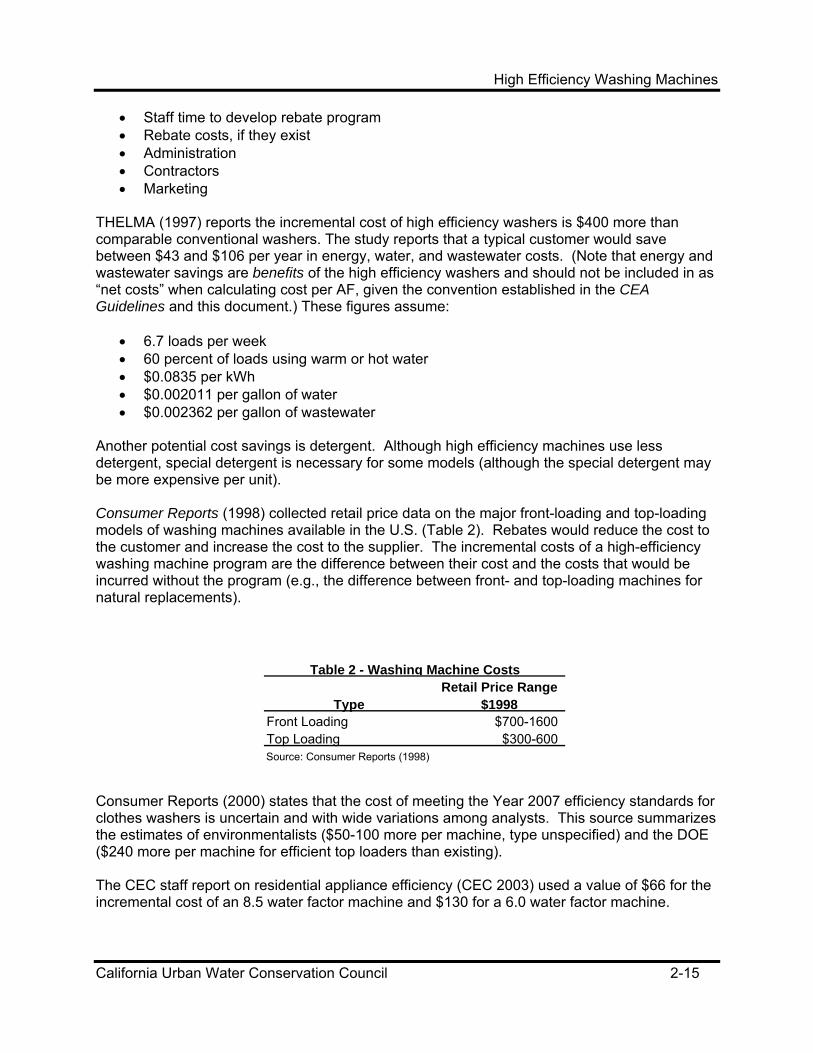
THELMA (1997) reports the incremental cost of high efficiency washers is $400 more than comparable conventional washers. The study reports that a typical customer would save between $43 and $106 per year in energy, water, and wastewater costs. (Note that energy and wastewater savings are benefits of the high efficiency washers and should not be included in as “net costs” when calculating cost per AF, given the convention established in the CEA Guidelines and this document.) These figures assume:
• 6.7 loads per week • 60 percent of loads using warm or hot water • $0.0835 per kWh • $0.002011 per gallon of water • $0.002362 per gallon of wastewater
Another potential cost savings is detergent. Although high efficiency machines use less detergent, special detergent is necessary for some models (although the special detergent may be more expensive per unit). Consumer Reports (1998) collected retail price data on the major front-loading and top-loading models of washing machines available in the U.S. (Table 2). Rebates would reduce the cost to the customer and increase the cost to the supplier. The incremental costs of a high-efficiency washing machine program are the difference between their cost and the costs that would be incurred without the program (e.g., the difference between front- and top-loading machines for natural replacements).
Consumer Reports (2000) states that the cost of meeting the Year 2007 efficiency standards for clothes washers is uncertain and with wide variations among analysts. This source summarizes the estimates of environmentalists ($50-100 more per machine, type unspecified) and the DOE ($240 more per machine for efficient top loaders than existing). The CEC staff report on residential appliance efficiency (CEC 2003) used a value of $66 for the incremental cost of an 8.5 water factor machine and $130 for a 6.0 water factor machine.
TypeRetail Price Range
$1998Front Loading $700-1600Top Loading $300-600Source: Consumer Reports (1998)
Table 2 - Washing Machine Costs

High Efficiency Washing Machines
California Urban Water Conservation Council 2-16
The U.S. EPA and DOE (2004) report that the typical price premium for an Energy Star certified washing machine is $300 however, all energy star rated machines are considered high efficiency in terms of their water use. A search of the keywords “Front Load Washers” at the Epinions.com shopping website brings up a list of machines that range in price from $520 to $1399. The reader is cautioned when regarding the use of these figures in analysis because they are not summarized with scientific methods. It is important to note that the costs of the high efficiency washers may differ for the varying perspectives of analysis. From the total society perspective, the cost is as described above—the difference between conventional washers and the high efficiency counterparts. For the customer, however, the costs might be less if a purchasing rebate program is in place. Likewise, the cost from the agency perspective is the cost of the rebate, which may not be the entire difference in costs—something less than $400 for each washer. Limitations As the market for high efficiency washers develops, the price difference between high efficiency and conventional machines is expected to decrease, so prices should be monitored by CUWCC to keep current. Confidence in Estimates High for estimates based on current market data. Less so for projections of future costs, although, costs are expected to decrease as production scale increases. 2.3.5 Water Savings Calculation Formula(s) Calculations S = Savings_per_Load * Water_Use_per_Load * Loads_per_Person * PPH where:
• S is savings (gpd/machine) • PPH is persons per household
Factors to Consider in Applying the Formula Loads per person may vary among demographic segments of the population, so a demographic distribution assessment could improve savings calculations. 2.3.6 Example Calculations Savings estimates from this numerical example are summarized in Table 3. When washing machines are shared, savings per machine can be estimated by multiplying savings times the
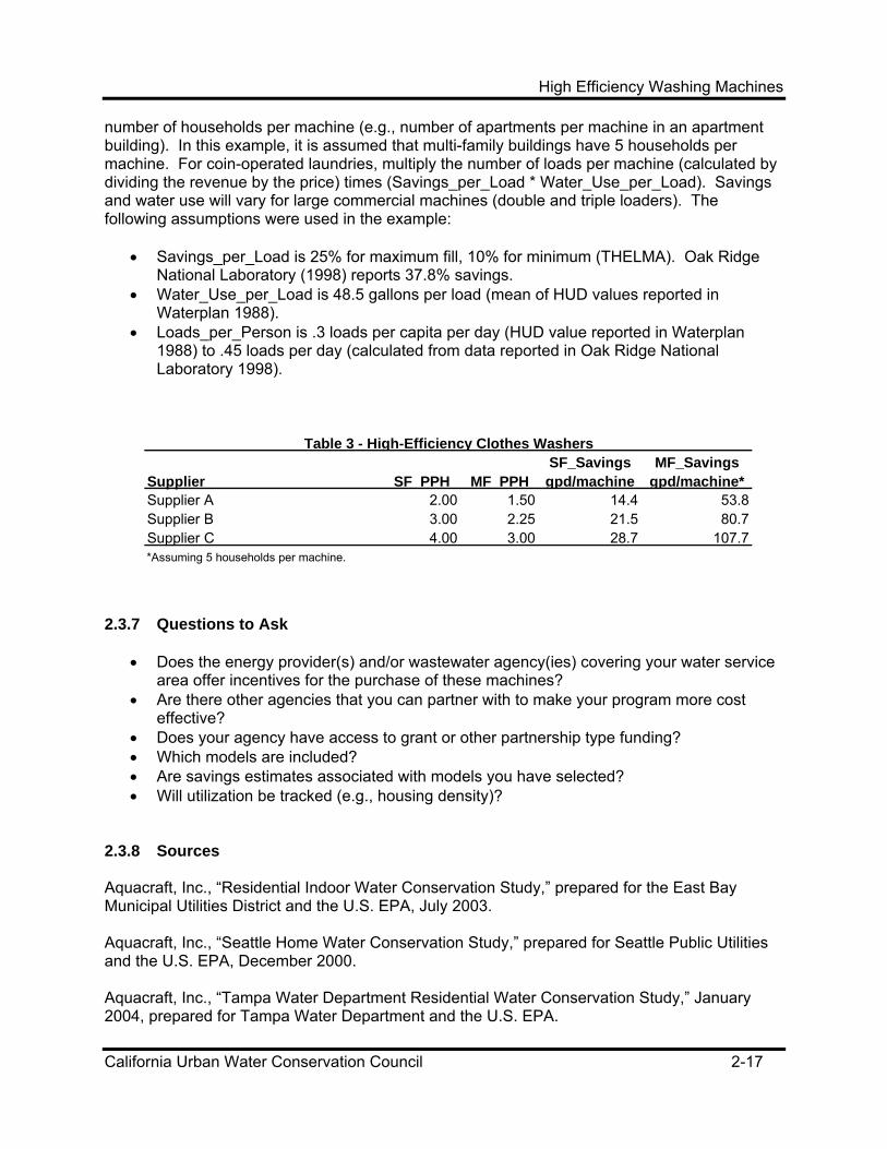
High Efficiency Washing Machines
California Urban Water Conservation Council 2-17
number of households per machine (e.g., number of apartments per machine in an apartment building). In this example, it is assumed that multi-family buildings have 5 households per machine. For coin-operated laundries, multiply the number of loads per machine (calculated by dividing the revenue by the price) times (Savings_per_Load * Water_Use_per_Load). Savings and water use will vary for large commercial machines (double and triple loaders). The following assumptions were used in the example:
• Savings_per_Load is 25% for maximum fill, 10% for minimum (THELMA). Oak Ridge National Laboratory (1998) reports 37.8% savings.
• Water_Use_per_Load is 48.5 gallons per load (mean of HUD values reported in Waterplan 1988).
• Loads_per_Person is .3 loads per capita per day (HUD value reported in Waterplan 1988) to .45 loads per day (calculated from data reported in Oak Ridge National Laboratory 1998).
2.3.7 Questions to Ask
• Does the energy provider(s) and/or wastewater agency(ies) covering your water service area offer incentives for the purchase of these machines?
• Are there other agencies that you can partner with to make your program more cost effective?
• Does your agency have access to grant or other partnership type funding? • Which models are included? • Are savings estimates associated with models you have selected? • Will utilization be tracked (e.g., housing density)?
2.3.8 Sources Aquacraft, Inc., “Residential Indoor Water Conservation Study,” prepared for the East Bay Municipal Utilities District and the U.S. EPA, July 2003. Aquacraft, Inc., “Seattle Home Water Conservation Study,” prepared for Seattle Public Utilities and the U.S. EPA, December 2000. Aquacraft, Inc., “Tampa Water Department Residential Water Conservation Study,” January 2004, prepared for Tampa Water Department and the U.S. EPA.
Supplier SF PPH MF PPHSF_Savings gpd/machine
MF_Savings gpd/machine*
Supplier A 2.00 1.50 14.4 53.8Supplier B 3.00 2.25 21.5 80.7Supplier C 4.00 3.00 28.7 107.7*Assuming 5 households per machine.
Table 3 - High-Efficiency Clothes Washers

High Efficiency Washing Machines
California Urban Water Conservation Council 2-18
California Energy Commission, “Update of Appliance Efficiency Regulations for Residential Clothes Washers,” Staff Report, publication # 400-03-021. Placed Online: September 19, 2003. CEE (1995) Consortium for Energy Efficiency High Efficiency Clothes Washer Initiative, “Program Description” with Appendices, December. Consortium for Energy Efficiency (CEE), “Residential Clothes Washer Initiative Fact Sheet,” URL: http://www.cee1.org/resid/seha/rwsh/rwsh-main.php3, downloaded July 2004. Consumer Reports, “What Will Energy Efficiency Cost?” URL: www.consumerreports.org, August 2000. CUWCC, “Projected Water Demand Reductions Derived From CEC Proposed Water Factor Standards,” statement filed by CUWCC, January 21, 2004. URL: http://www.cuwcc.org. Epinions.com, “Front-Load Washer Prices,” URL: www.epinions.com, downloaded April 2004. Fryer, James, “THELMA Update,” Memorandum, Marin Metropolitan Water District, November 21, 1995. HUD (1984) U.S. Department of Housing and Urban Development, Office of Policy Development and Research, Building Technology Division, Survey of Water Fixture Use, Brown and Caldwell Consulting Engineers, March. Mitchell, David (1998), “Ad Hoc H-Axis Committee Interim Savings Recommendations,” memo prepared for CUWCC, March. Oak Ridge National Laboratory (1998) “Bern Clothes Washer Study: Final Report,” prepared for the U.S. Department of Energy, March. Oak Ridge National Laboratory (ORNL), “The Boston Washer Study,” prepared for the U.S. Department of Energy, URL: www.eere.energy.gov, January, 2003. Pacific Northwest National Laboratory (PNNL), “The Save Water and Energy Education Program: SWEEP: Water and Energy Savings Evaluation,” prepared for the U.S. Department of Energy, May 2001. Pugh, C.A., and J.J. Tomlinson, "High-Efficiency Washing Machine Demonstration, Bern, Kansas," proceedings of Consev99, 1999. THELMA (1995a) “THELMA The High Efficiency Laundry Metering & Marketing Analysis,” Executive Summary and Chapter 5. THELMA (1995b) Diekmann, J. and W. Murphy, “Laboratory Testing of Clothes Washers,” prepared by Arthur D. Little, Inc. for the EPRI Customer Systems Group, Final Report, December.

High Efficiency Washing Machines
California Urban Water Conservation Council 2-19
THELMA (1997) “THELMA Impact Analysis,” EPRI Retail Market Tools and Services, prepared by SBW Consulting, Hagler Bailly Consulting, Dethman & Associates, and the National Center for Appropriate Technology, March. U.S. EPA and Department of Energy, “Energy Star Qualified Clothes Washers,” URL: www.eere.energy.gov, downloaded July 2004. Waterplan (1988) Synergic Resources Corporation, “Waterplan Benefit/Cost Analysis Software for Water Management Planning,” prepared for California Department of Water Resources, November.

Hot Water Recirculation on Demand
California Urban Water Conservation Council 2-20
2.4 Hot Water Recirculation On Demand (Residential) 2.4.1 Device/Activity Description Hot water recirculation-on-demand systems deliver hot water to a faucet or shower without having to drain the cold water in the pipes between the water heater and the fixture. To re-circulate “on demand” using a valve and a pump, the device temporarily opens a loop between the hot and cold water lines, pumps the cold water sitting in the hot water pipe into the cold water pipe and back into the hot water heater tank. When the hot water in the hot water pipe arrives at the unit and the water temperature rises, pumping stops, the loop closes, and the plumbing system is returned to conventional functioning--now with hot water at the tap. To facilitate re-circulate on demand, the system can be started with buttons or remote control. Related technologies not included in this section include 1) continuous hot water recirculation, more typical in the commercial or multi-family residential sectors; 2) hot water heated on demand using a tankless heater; and 3) hot water heated on demand at the point of use, such as an instant hot water faucet for tea and coffee, or a hot water unit for a remote bathroom. 2.4.2 Applicable BMPs Hot water recirculation-on-demand systems are related to BMP 2 – Residential Plumbing Retrofits. Although not mentioned in the BMP, the units are a type of plumbing retrofit. It is not clear that this technology could be used toward compliance with BMP 2. 2.4.3 Available Water Savings Estimates Summary of Individual Studies The California Energy Commission (CEC) analyze water and energy savings from hot water recirculation on demand units in residential settings (Klein 2004). Water savings depend on the number of "cold start" hot water runs from the water heater to the faucet or shower. Water is saved only when water in the pipe is cold, not when water is already hot. Furthermore, although runs per day will clearly be higher in households with more persons, it is not clear that "cold-start" runs will increase in proportion to household residents; the greater the frequency of use of a fixture, the more likely that it is already hot. In most cases, un-insulated pipes cool down in about 10 minutes. Not all houses in a region will be able to realize the full savings from the hot water recirculation-on-demand system because of their plumbing design. Water savings is dependent on the volume in the pipe between the water heater and the faucet. The CEC measurements indicate that approximately twice the pipe volume is needed to warm up the water at the faucet because of the need to warm up the pipes along the way. The run times for hot water lines need to be broken down by size of pipes (½” versus ¾”), since size is one of the large factors in determining how much water will be used to get hot water. For example, 5.52 feet of ½ inch “K” copper pipe holds one cup of water; only 2.76 feet of ¾ inch

Hot Water Recirculation on Demand
California Urban Water Conservation Council 2-21
pipe is needed to hold one cup, so savings estimates will be approximately half as much with for ½” lines as for ¾” lines. Klein and Lutz (2004) analyze water loss in residential settings. Although the study does not estimate savings, it does cover the sources of water loss in depth, including losses that are meant to be mitigated by hot water recirculation-on-demand systems. See also Klein 2004. The Palo Alto study (ORNL 2002) of hot water recirculation on demand found “water savings for a household of four occupants varied from about 900 gallons to about 3000 gallons per point of use, per year. Point of use is a single location at a home--for example a faucet where hot water is available. Based on these figures, the water savings in a home with four points of use, on the average, would be 3,600 to 12,000 gallons per year.” Santa Clara Valley Water District (2002) found per household water use decreased by 2% (8.6gpd) in the treatment year relative to the control year. In Phase II of the study, discretionary water use decreased by .6 gallons per day. Neither of these values were reported to be statistically significant, in part due to small sample sizes, but also because the systems were not activated frequently—only three times per day on average. Advanced Conservation Technology Metlund Inc. has conducted a small-scale survey of households that have been retrofitted with hot water recirculation-on-demand units. A four-page survey was sent to 30 randomly selected households. Respondents self reported by following directions on the survey on how to measure water loss (e.g., respondents measured length of wait time for water to get hot, and flow rate of device by measuring with a quart container). A total of 26 out of the 30 households responded. Persistence No study considering the persistence of savings from hot water recirculation-on-demand units has been found. Limitations An important limitation is data regarding the number and type of sites with plumbing that is configured to take advantage of the hot water demand system. Confidence in Estimates Medium. More evidence needs to be developed regarding the number existing plumbing configurations that would effectively save water if retrofitted with hot water recirculation on demand systems, the number of cold-start runs per person per day, how the number of cold-start runs scales as more people live in the same household (scaling factor), and the mean and distribution of savings per run that can be expected under different circumstances. 2.4.4 Program and Device/Activity Cost Estimates Program Costs

Hot Water Recirculation on Demand
California Urban Water Conservation Council 2-22
One estimate of costs of hot water recirculation on demand units is $500 per unit installed (Stranz 1996). These cost figures are derived from information supplied by the manufacturer. ACT Metlund indicates that the latest model reduces installation labor time by 50 percent compared to previous models, and that its cost is $208 for the parts without labor (www.chilipeperapp.com 1999). The Palo Alto study (ORNL 2002) states the cost of the hot water circulation on demand system used in the study was $399 (it does not specify whether this included installation costs). ORNL (2003) estimated the cost of adding a recirculation on demand system to an existing house is $694 for the parts and labor. The cost of including the system to new home construction, with design improvements, was estimated to be $1880. This includes un-insulated copper pipe in the lowest cost sample house. Water waste per month ranged from 68 to 308 gallons—the maximum technical potential savings. Limitations (1) The savings figures are for retrofits. If the house is plumbed to take full advantage of the hot water demand unit, then greater savings are likely to occur. One important savings factor is the distance between the fixture (e.g., shower or sink) and the trunk water line from the water heater. Short branches are better. Only one demand unit is needed if the fixtures are arrayed in series along the trunk line (the unit is installed at the furthest point from the water heater). If a radial design is used, then a unit is needed at the end of each branch, which would be costly. Other factors that influence savings include the distance between the water heater and the fixtures (most houses in California have water heaters in the garage), and pipe location and insulation (pipes are often un-insulated and in attics or basements). (2) Most of these devices are installed in the single-family residential sector, although the multi-family sector has potential. (3) Some new homes are built with re-circulating hot water systems similar to those used in the commercial sector. In these houses, this technology would not save additional water if hot water is circulated continuously back through the dedicated hot water return line. It could however, be used to save energy by operating the re-circulating system on-demand rather than continuously. As explained above, pipe diameter is also an important variable. Confidence in Estimates Medium-Low. Costs will depend on plumbing layout. 2.4.5 Water Savings Calculation Formula(s) Calculations S = Cold_Start_Hot_Water_Runs * Savings_per_Run * Plumbing_Factor where:
• S is savings (gpd/hot water demand unit) • Cold_Start_Hot_Water_Runs = PPH * Hot_Water_Runs * Scale_FactorPPH • Savings_per_Run is the water savings per hot water run. • Hot_Water_Runs is the number of times the water is heated up at the faucet.

Hot Water Recirculation on Demand
California Urban Water Conservation Council 2-23
• Scale_Factor is the degree to which hot water runs are reduced as persons per household increases, because the likelihood of water already being hot is higher (judgment; CEC 1995).
• PPH is persons per household. • Plumbing_Factor is represents the ability house to realize savings because of the
configuration of the plumbing system and its ability to take advantage of the hot water demand unit (e.g., 1/2 get 50 percent savings, the other half get 100%, so together the plumbing factor is .75).
Factors to Consider when Applying the Formula Additional data would allow stratification that could be used to develop separate models for different site types. Example Calculations The following assumptions were used in the sample calculations:
• Savings_per_Run is a mean of 4.0 gallons per hot water run; with a range of 2-12 gallons per run (ACT Metlund 1995; CEC 1995).
• Hot_Water_Runs has a mean of 6 hot water runs per day per person and a range of 2-10 (based on ACT Metlund 1995; CEC 1995; Davis Energy Group 1988).
• Scale_Factor is .8 is the degree to which hot water runs are reduced as persons per household increases, because the likelihood of water already being hot is higher (judgment; CEC 1995).
• Plumbing_Factor is .75. Table 1 shows the results of using these assumptions, and another plausible set of assumptions. It demonstrates the need for better data; savings estimates can be widely different under different conditions. Note importantly, that the values in this example are for ¾ inch lines; savings would be about half as much for ½ inch lines.
Supplier SF PPH
Cold-Start Hot Water Runs
(runs/day/unit)Savings
g/day/unitSupplier A* 2.0 7.7 23.0Supplier B* 3.0 9.2 27.6Supplier C* 4.0 9.8 29.5Supplier A** 2.0 8.0 6.0Supplier B** 3.0 12.0 9.0Supplier C** 4.0 16.0 12.0*saving per run: 4 gal; runs per person per day 6; scale factor .8; plumbing factor .75**saving per run: 1 gal; runs per person per day 4; scale factor 1; plumbing factor .75
Table 1 - Hot Water Demand Unit(savings gpd/unit)

Hot Water Recirculation on Demand
California Urban Water Conservation Council 2-24
2.4.6 Questions to Ask
• Is the hot water demand unit installed at the time of construction or retrofit? • Is the plumbing configuration closer to an “in-line” or “hub-and-spoke” layout? • How many pump and controller units would be needed to use the system at the most
important output locations (bathroom and kitchen)? • What is the pipe diameter?
2.4.7 Sources Acker, Larry (1995), ACT Metlund Systems, Telephone interview, 21 December. ACT Metlund Systems (1995), “Home Test Audit Report,” Metlund Hot Water Demand Systems, July 18. Davis Energy Group (1988), “Residential Water Heating Study: Technical Report,” Use Pattern Assumptions in Appendix F, Table F-2, prepared for the California Energy Commission, Contract Number 400-88-003 (1988 contract), as reported by Klein (1995). Klein, G., “Saving Energy and Water in Residential Hot Water Systems,” AWWA 2004 Water Sources Conference Proceedings. Klein, G., and J. Lutz, “Hot Water Distribution Losses in Residential Buildings: Draft Scoping Study,” California Energy Commission and Lawrence Berkeley National Laboratory, August 2004 Oak Ridge National Laboratory (ORNL) “Water and Energy Savings using Demand Hot Water Recirculating Systems in Residential Homes: A Case Study of Five Homes in Palo Alto California,” with the City of Palo Alto Public Utility Commission, October 2002. Oak Ridge National Laboratory, “Evaluation of Residential Hot Water Distribution Systems” Draft Final Report prepared for the Davis Energy Group and the California Energy Commission, May 2003. Oak Ridge National Laboratory, “Residential Hot Water Demand System,” for the City of Palo Alto Public Utilities and the U.S. Department of Energy, updated January 2003, URL: www.eere.energy.gov. Santa Clara Valley Water District, “Hot Water Re-circulation Pilot Study,” March 2002. Stranz, Blake (1996), “Hot Shot: Innovative Hot Water System Saves Money, Energy and Time,” America How-To, March/April. www.chilipeperapp.com (1999), Chilipepper Hot Water Appliance.

Metering
California Urban Water Conservation Council 2-25
2.5 Universal Metering and Multi-Family Submetering 2.5.1 Device/Activity Description In general, meters are instrumental to a number of conservation efforts because they provide information on water use to consumers. Universal metering for conservation consists of installing water meters in existing customer sites where they do not currently have meters, and assuring new construction is metered. Installing a meter where none exists provides the customer the information needed to recognize volumetric price incentives. An associated activity is the replacement of existing meters that are not operating properly. Replacing meters that are not operating properly may “true up” the price signal sent to customers.7 Meters can also be added to individual units in a multi-family building; so called “submetering” allows separate household-level water usage measurement where there was previously only a master meter. Note that this section includes submetering but not ratio utility billing systems (RUBS). 2.5.2 Applicable BMPs
• BMP 4 – Metering with Commodity Rates. • Metering is a necessary condition for implementing BMP 11 – Pricing.
2.5.3 Available Water Savings Estimates Summary of Individual Studies Speedwell (1994) analyses data from a sample of 590 multi-family buildings in New York City and a sample of 676 multi-family buildings in Jamaica, New York. The Jamaica service area was metered and the New York City buildings were not. A statistical model was developed, regressing housing density, median income in the census tract, building size water use, and a dummy variable for Jamaica service area on water use. Controlling for these independent variables, metered billing resulted in a 36 percent decrease in water use, which the authors attribute to the metering of water consumption. Bishop and Weber (1995) report the results of a statistical analysis of Denver’s universal metering program. The average annual water savings is reported as 28 percent, with a summer peak seasonal reduction of 38.4 percent in 1991. The authors cite landscape irrigation as the reason for the large summer savings with metering. The authors report that controlling for season, weather, and the effect of metering and conservation practices, 98 percent of the monthly variation is explained in the model. However, savings estimated in the statistical model cannot be separated from savings from concurrent programs used to promote the installation of conservation devices, such as bathroom retrofits. The savings effect is also not separated from
7 Metering can also be used to separately measure indoor from outdoor use. In this document, we refer to these meters as “dedicated [landscape] meters” and this topic is covered in the section on Large Landscape Measures.
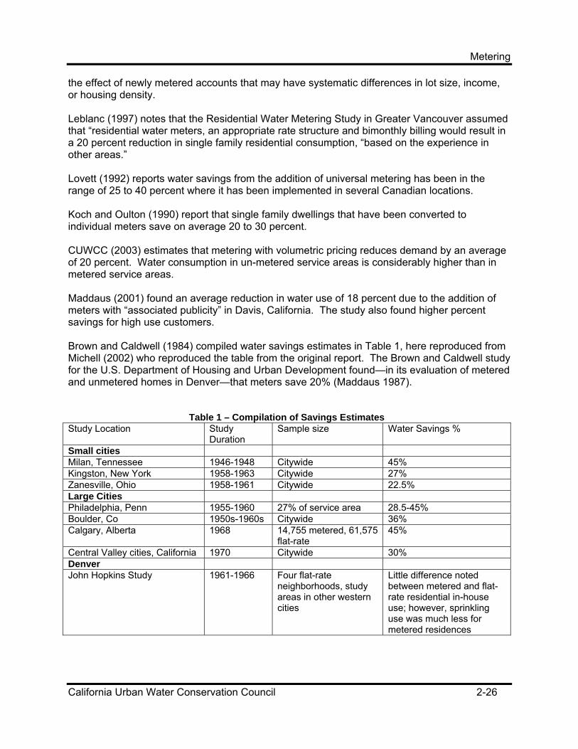
Metering
California Urban Water Conservation Council 2-26
the effect of newly metered accounts that may have systematic differences in lot size, income, or housing density. Leblanc (1997) notes that the Residential Water Metering Study in Greater Vancouver assumed that “residential water meters, an appropriate rate structure and bimonthly billing would result in a 20 percent reduction in single family residential consumption, “based on the experience in other areas.” Lovett (1992) reports water savings from the addition of universal metering has been in the range of 25 to 40 percent where it has been implemented in several Canadian locations. Koch and Oulton (1990) report that single family dwellings that have been converted to individual meters save on average 20 to 30 percent. CUWCC (2003) estimates that metering with volumetric pricing reduces demand by an average of 20 percent. Water consumption in un-metered service areas is considerably higher than in metered service areas. Maddaus (2001) found an average reduction in water use of 18 percent due to the addition of meters with “associated publicity” in Davis, California. The study also found higher percent savings for high use customers. Brown and Caldwell (1984) compiled water savings estimates in Table 1, here reproduced from Michell (2002) who reproduced the table from the original report. The Brown and Caldwell study for the U.S. Department of Housing and Urban Development found—in its evaluation of metered and unmetered homes in Denver—that meters save 20% (Maddaus 1987).
Table 1 – Compilation of Savings Estimates Study Location Study
Duration Sample size Water Savings %
Small cities Milan, Tennessee 1946-1948 Citywide 45% Kingston, New York 1958-1963 Citywide 27% Zanesville, Ohio 1958-1961 Citywide 22.5% Large Cities Philadelphia, Penn 1955-1960 27% of service area 28.5-45% Boulder, Co 1950s-1960s Citywide 36% Calgary, Alberta 1968 14,755 metered, 61,575
flat-rate 45%
Central Valley cities, California 1970 Citywide 30% Denver John Hopkins Study 1961-1966 Four flat-rate
neighborhoods, study areas in other western cities
Little difference noted between metered and flat-rate residential in-house use; however, sprinkling use was much less for metered residences

Metering
California Urban Water Conservation Council 2-27
Green’s Thesis 1972 Three of four flat-rate areas from John Hopkins project plus surrounding metered areas
13-30%
Beck Report 1966-1968 Two flat-rate areas plus two metered areas from Aurora
Results similar to John Hopkins study.
Bryson’s Thesis 1971 90,290 flat-rate residential service, 19,080 metered residences
25%
Source: Reproduced from Brown and Caldwell (1984) as reported in Mitchell (2002) Lund (1984) compiled water savings estimates in Table 2, here reproduced from Mitchell (2002) who reproduced the table from the original report.
Table 2 – Estimates of Use Reduction from Water Metering City Year % Reduction Reference Kingston, NY 1958-63 20% Cloonan, 1965 Philadelphia 1955-60 28% Cloonan, 1965 Boulder, CO 1960-65 40% Hanke & Flack, 1968 various, USA 1963-65 34% Howe & Linaweaver, 1967 Israeli apts. - 14-34% Darr et al., 1975 Malmoe, Sweden 1980 34% Hjorth, 1982 Solomon Is. 1969-70 50% Berry, 1972 Flyde, UK 1970-72 10% Smith, 1974 Malvern, UK - 20% Smith, 1974 Malvern, UK 1970-75 6% Phillips & Kershaw, 1976
Submetering Rosales, Weiss, and DeOreo (2002) report savings of 7 to 12 percent from submetering in two mobile home communities. Griffin (2001) estimates demand drops from 6 to 39 percent with individual utility billing. Industrial Economics (1999) reported median savings values of 39 percent in terms of gallons per year per resident, and 18 percent in terms of gallons per year per square foot, with common areas included. Aquacraft (2004) found, in a national study, that submetering saved 15.3 percent, or equivalently 21.8 gallons per unit per day. The City of Portland (undated) reports 15 percent less water per resident in an apartment building with submetering compared to a similar building without submetering. Goodman (1999) and Goodman and Lee (1999) estimate that water consumption will drop by 50 percent when a customers go from zero marginal cost per unit of water (flat un-metered rate) to the national average of $21.56 for the first 1,000 cubic feet.

Metering
California Urban Water Conservation Council 2-28
Koch (undated) estimated savings in warm water consumption are 52% as compared to the norm, and 55% as compared to the real consumption prior to the installation of the energy conservation systems. The results for cold water savings are 68% and 37% respectively. The average heat economies are 45% and 23% respectively. Source: Reproduced from Lund (1984) as reported in Mitchell (2002) Persistence No study considering the persistence of savings from water metering has been found. Limitations None of the studies have fully controlled for all possible and reasonable explanatory variables. In particular, other conservation programs may have been concurrent with the metering program evaluations. Confidence in Estimates Low. Future efforts should include empirical measurement of water savings considering an appropriate range of explanatory variables. It is important to consider the interactive effect of metering along with other conservation programs; savings from metering and other conservation programs may not be additive. Savings may also be considerably different depending on the amount of outdoor use. 2.5.4 Program and Device/Activity Cost Estimates Program Costs Participant program costs may include:
• Meter installation cost, if not paid by the supplier.
Supplier program costs may include:
• Staff time to develop meter program and new rates structure • Meter and installation costs, if the supplier pays. • Administration • Contractors • Marketing
Denver Water Department (1993) reports the average cost per meter setting to be $425, including purchase, installation, repair of deteriorating lines, and public education. Bishop and Weber (1995) report costs in the range of $250 to $750 per meter for purchase and installation. The cost to install a meter in a new construction residence is cited as $175.

Metering
California Urban Water Conservation Council 2-29
Leblanc (1997) reports that the cost of meter purchase and installation is $210 for indoor and $450 for outdoor. [We assume Canadian dollars, although it is not specified in the article]. Westerling and Hart (1995) develop a cost minimization model to determine the optimal period of time between meter replacements. Their sample calculations indicate a range between 7 and 14 years. CUWCC (2003) report the costs of the installing meter retrofits vary depending on the size of the meter. For example, costs are in the range of $500-$1000 for single-family dwellings in Central Valley/per meter, and $500-$3000 for multi-family dwellings & commercial connections. There are additional costs to read the meter and bill the residential customer with a volumetric rate. Mitchell (2002) assembled the estimates of water meter installation costs in Table 3.
Table 3 -- Estimates of Use Reduction from Water Metering Water Supplier Region Avg. Cost Per Meter
Installation Notes
Sacramento Suburban
Sacramento Valley
$910 per residential meter Most residential connections in backyards. Meter, box, and meter setter cost $240. Installation, which includes up to 28 sq ft of landscape restoration, is $670.
San Juan Water District
Sacramento Valley
$246 to install residential meter and box plus additional $207 if service upgrade required. Combined cost is $453.
Cost information provided by field operations manager for San Juan Water District
Citrus Heights Water District
Sacramento Valley
$890 (contractor install) $533 (district staff install) These are costs for residential meters
Based on 6,996 contractor and 2,056 district staff installations. Cost for contractor installation includes district inspection cost of about $40/meter.
City of Carmichael Sacramento Valley
3/4”, 1” - $1,500 11/2”, 2” - $2,000 3” - $1,775 4” - $2,500
Detailed cost spreadsheet with itemization available.
City of Roseville Sacramento Valley
<$775 per residential meter Estimated cost was $775, but actual cost turning out to be somewhat less
Fair Oaks Water District
Sacramento Valley
$700 per residential installation
Install cost can run as high as $1,500 when landscape or hardscape need to be replaced.
City of Davis Sacramento Valley
$450 per residential installation (1994 dollars)
All installations were front easements.
City of Fresno San Joaquin Valley
$300-$350 per retrofitted residential meter (1990 dollars); $150 per new residential installation
Source: Reproduced from Mitchell (2002)

Metering
California Urban Water Conservation Council 2-30
Aquacraft (2004) reported cost in new construction of $125 for meter, transmitter, and installation ($300 for retrofits), $25 for receiver, computer, and software, and an annual service fee of $36. Limitations Payments conventions may vary from supplier to supplier. For example, where new development takes place, the developer and new owners, not by the supplier, may incur metering cost. Alternatively, the supplier may incur retrofit costs. Confidence in Estimates Low. 2.5.5 Water Savings Calculation Formula(s) S = Household_Water_Consumption * Savings_Percent where:
• Household_Water_Consumption is the pre-metering consumption • Savings_Percent is the percent savings assumed to result from metering
Factors to Consider in Applying the Formula Household water consumption may variable considerably by socioeconomic status, climate, and landscape variation. 2.5.6 Example Calculation(s) With available information, savings can be calculated by taking a service area water use and multiplying by percentage savings. Table 4 shows sample calculations for different levels of water use.
2.5.7 Questions to Ask
Water Use (gpd) 20% 30% 40%20 4 6 840 8 12 1660 12 18 2480 16 24 32100 20 30 40120 24 36 48
Table 4 - Savings from Meters (gpd)Percent Savings

Metering
California Urban Water Conservation Council 2-31
• Are there other agencies that you can partner with to make your program more cost effective?
• Does your agency have access to grant or other partnership type funding? • Are current un-metered connections in easements behind the residences or in front in
public property? (1) • If in easements behind residences, does your agency maintain leak histories, which
would indicate the need to replace the easement mains? (1) • Are there currently shutoff valves with spacers (for future meter installations) inside
meter boxes for your un-metered connections? (1) • If service line shutoff valves are not already in place, are the locations of your agencies
service lines known where meter boxes, shut off valves and meters are to be installed? (1)
• What is the typical distance from main to meter? (1) • Based on the meter manufacturer chosen, what is the availability and cost of remote
(radio frequency) reading? (1) • What is the cost of meters in bulk? (1) • Would your agency install meters or use contractors? (1) • Can your agency bill metered customers prior to completing your meter program for all
customers? • Will your agency meter all customers within the shortest cost effective period, or spread
implementation over the 10 years allowed by the BMP? (1) • Would your agency read meters on a monthly or bimonthly basis? (2) • Does your agency currently have a metered billing system, or would such a system have
to be designed and/or purchased? (2) • Is the water bill designed to communicate water consumption and compare like months
or periods for current and past years? (2) • What is the age of the housing stock (opportunity for leak detection)? • How often is meter accuracy checked?
(1) Your metering cost will vary substantially based on the responses you obtain for these
questions. Hint - your operations department should be able to provide this information or direct you to those within your agency who can.
(2) Your operational cost will vary depending on your responses to these questions. Hint - your accounting and/or your information systems department(s) should be able to provide you with these responses.
2.5.8 Sources American Water and Energy Savers, “Water Submetering for Commercial Property,” URL: www.americanwater.com, April 2003. American Water Works Association, “Water Meters: Selection, Installation, Testing, and Maintenance, 4th Edition, (M6),” 1999. Aquacraft, Inc, et al., “National Multiple Family Submetering and Allocation Program Study” with East Bay Municipal Utility District, 2004.

Metering
California Urban Water Conservation Council 2-32
Berry, N.S.M. (1972), “The Effect of Metering on Water Consumption in Honiara-British Solomon Islands,” Journal, of the Institution of Water Engineers, Vol. 26, No. 7 (October), pp. 375-380 Bishop, W. J., and J.A. Weber (1995), “Impacts of Metering: A Case Study at Denver Water,” prepared for the 20th Congress IWSA, Durban, South Africa, September. Brown & Caldwell (1984), “Effect of Water Meters on Water Use,” Prepared for U.S. Department of Housing and Urban Development, Contract H-5230. California Urban Water Conservation Council, “AB 514 (Kehoe): Water Meters – Support, Hearing: Senate Agriculture and Water Resources – July 1, 2003.” Letter from Mary Ann Dickinson to Senator Michael Machado, June 24, 2003. City of Kamloops (2001), “Water Use Efficiency Committee Final Report, Appendix E.” City of Portland Bureau of Water Works, “Multi-Family Housing Water Conservation Manual: A Practical Guide to Saving Water and Money,” undated. Cloonan, E.T. (1965), “Meters Save Water, “ in Modern water Rates, Battenheim Publishing Co., N.Y. Darr, Peretz, Stephen L. Feldman, and Charles S. Kamen (1975), “Socioeconomic Factors Affecting Domestic Water Demand in Israel,” Water Resources Research, Vo. 11, No. 6, pp. 805. Denver Water Department (1993), "Final Report: Universal Metering Project, “Customer Services Section, Public Affairs Division, March. Goodman, J. (1999), “Water Conservation From User Charges in Multifamily Rental Housing,” National Multi Housing Council, June 1999. Goodman, J. and E. Lee (1999), “Multifamily Housing: Direct Billing Spurs Water Conservation,” National Multi Housing Council, September 1999, URL: www.nreionline.com. Griffin, W., “Utility Billing Programs Can Lower Housing Costs,” National Submetering & Utility Allocation Association Forum, June 2001, URL: www.nsuaa.org. Hanke, Steve H. and Ernest Flack Jr. (1968), “Effects of Metering Urban Water,” Journal of the American Water Works Association, Vol. 60. Hjorth, Peder (1982), Identifying och Analys av Faktorer Vilka Styr Vattenforbrukningen och Dess Variationer, Report No. 3068, Department of Water Resources Engineering, Lund Institute of Technology, University of Lund, Lund, Sweden, 47. pp. Howe, Charles W. and F.P. Linaweaver Jr. (1965), “The Impact of Price on Residential Water Demand and Its Relation to System Design, “Water Resources Research, Vol. 1. Industrial Economics, Inc., “Submetering, RUBS, and Water Conservation,” for National Apartment Association and National Multi Housing Council, June 1999.

Metering
California Urban Water Conservation Council 2-33
Koch, R. N. and R.F. Oulton (1990), “Submetering: Conservation’s Unexplored Potential,” AWWA Conference Proceedings Koch, T., “Water And Heat Savings In Russian Apartment Buildings - Results Of The Dubna Project,” Institute for Energy Policy, Undated. Las Vegas Valley Water District, “The Impacts of Submetering on Water Usage at Two Mobile Home Communities in Las Vegas, Nevada,” with Aquacraft Inc., Proceedings of the American Water Works Association Water Sources Conference, 2002. Leblanc, L., et al. (1997), “Is Residential Metering Cost-Beneficial in Water-Rich Greater Vancouver?” Conference Proceedings of the American Water Works Association, Pacific Northwest Section Lovett, D. (1992), “Water Conservation Through Universal Metering,” 44th Annual Convention of the Western Canada Water and Wastewater Association Proceedings. Lund, J. R. (1986) “Metering Utility Services: Theory and Water Supply Applications,” Water Resources Series Technical Report No. 103, University of Washington, Dept. of Civil Engineering. Maddaus, L.A., “Effects Of Metering On Residential Water Demand for Davis California,” Master’s Degree Project for the Civil & Environmental Engineering Department, University Of California, Davis, March 2001. Maddaus, W.O., “The Effectiveness of Residential Water Conservation Measures,” Journal AWWA, March 1987. Mitchell, D.M., “Cost of Meter Installation for Different Areas of CA,” Memo to Eric Poncelet, CONCUR, Inc., December 13, 2002. Mitchell, D.M., “Water Conservation Benefits Of Metering/Volumetric Billing,” Memo to Eric Poncelet, CONCUR, Inc., October 21, 2002. National Submetering & Utility Allocation Association, “Bibliography Of Utility Submetering and Allocation Industry Information,” URL: www.nsuaa.org, undated, downloaded August 2004. Phillips, J.H. and C.G. Kershaw (1976), “Domestic Metering - An Engineering and Economic Appraisal,” Journal of the Institution of Water Engineers and Scientists, Vol. 30, No. 4, pp. 203-216. Rosales, J., C. Weiss, and W. DeOreo, “The Impacts of Submetering on Water Usage at Two Mobile Home Communities in Las Vegas, Nevada,” 2002 Water Sources Conference Proceedings. Seattle Public Utilities, “Sub-Metering: The Next Big Conservation Frontier?” presented at Conserv99, 1999. Smith, R.J. (1974), “Some Comments on Domestic Metering,” Journal of the Institution of Water Engineers, Vol. 28, No. 1, pp. 47-53.

Metering
California Urban Water Conservation Council 2-34
Speedwell, Inc. (1994), “The Impact of Metered Billing for Water and Sewer on Multifamily Housing in New York,” prepared for the New York City Department of Environmental Protection and the New York City Rent Guidelines Board, September. Water Resources Engineering Inc., “Overview of Retrofit Strategies: A Guide for Apartment Owners and Managers,” for U.S. Department of Housing and Urban Development, May 2002. Water Resources Engineering Inc., “Retrofitting Apartment Buildings to Conserve Water,” for U.S. Department of Housing and Urban Development, May 2002. Westerling, D.L., and F.L. Hart (1995), “A Rational Approach for Making Decisions on Replacement of Domestic Water Meters,” Journal NEWWA, December.

Conservation Pricing
California Urban Water Conservation Council 2-35
2.6 Conservation Pricing 2.6.1 Device/Activity Description Conservation pricing provides incentives to customers to reduce water use. Applicable BMPs
• BMP 4 – Metering and Commodity Rates—metering is a prerequisite for volumetric pricing
• BMP 11 – Conservation Pricing 2.6.2 Available Water Savings Estimates The report from the first phase of the CUWCC (1994) urban water rates project, Setting Urban Water Rates for Efficiency and Conservation: A Discussion of the Issues provides a good introduction to understanding how urban water demand responds to price. Table 1 provides a summary drawn from Chapter 1 of the Phase I report.
Table 1: Lessons about how Rates affect Water Demand Lesson 1: Rates influence demand. Lesson 2: “Price elasticity” is the percentage change in demand induced by a one percent
change in price, all other factors being constant. Lesson 3: Demand can be thought of as the sum of demands for different end uses of water. Lesson 4: Demand for outdoor uses is more price-elastic than demand for indoor uses. Lesson 5: Demand for water during peak (summer) periods is greater than demand during
off-peak (winter) periods. Lesson 6: Residential water demand is relatively inelastic. The response of residential
demand to rate changes, though not zero, is relatively small. Lesson 7: Demand is more elastic in the long run than in the short run. Lesson 8: Demand is influenced by forces other than price—including population growth,
the economic cycle, weather fluctuations, and income growth. Lesson 9: The response of demand is more difficult to predict for large changes in price.
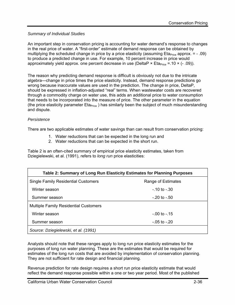
Conservation Pricing
California Urban Water Conservation Council 2-36
Summary of Individual Studies An important step in conservation pricing is accounting for water demand’s response to changes in the real price of water. A “first-order” estimate of demand response can be obtained by multiplying the scheduled change in price by a price elasticity (assuming EtaPrice approx. = - .09) to produce a predicted change in use. For example, 10 percent increase in price would approximately yield approx. one percent decrease in use (DeltaP × EtaPrice =.10 × (- .09)).
The reason why predicting demand response is difficult is obviously not due to the intricate algebra—change in price times the price elasticity. Instead, demand response predictions go wrong because inaccurate values are used in the prediction. The change in price, DeltaP, should be expressed in inflation-adjusted “real” terms. When wastewater costs are recovered through a commodity charge on water use, this adds an additional price to water consumption that needs to be incorporated into the measure of price. The other parameter in the equation (the price elasticity parameter EtaPrice ) has similarly been the subject of much misunderstanding and dispute. Persistence There are two applicable estimates of water savings than can result from conservation pricing:
1. Water reductions that can be expected in the long run and 2. Water reductions that can be expected in the short run.
Table 2 is an often-cited summary of empirical price elasticity estimates, taken from Dziegielewski, et al. (1991), refers to long run price elasticities:
Table 2: Summary of Long Run Elasticity Estimates for Planning Purposes
Single Family Residential Customers Range of Estimates
Winter season -.10 to -.30
Summer season -.20 to -.50
Multiple Family Residential Customers
Winter season -.00 to -.15
Summer season -.05 to -.20
Source: Dziegielewski, et al. (1991)
Analysts should note that these ranges apply to long run price elasticity estimates for the purposes of long run water planning. These are the estimates that would be required for estimates of the long run costs that are avoided by implementation of conservation planning. They are not sufficient for rate design and financial planning. Revenue prediction for rate design requires a short run price elasticity estimate that would reflect the demand response possible within a one or two year period. Most of the published

Conservation Pricing
California Urban Water Conservation Council 2-37
empirical literature on price elasticity focuses on long run estimates. Estimates of short run price elasticities are not as common. Table 3 is from CUWCC’s Handbook on Designing, Evaluating, and Implementing Conservation Rate Structures. It provides the following recommended ranges for short run price response:
Table 3: Short Run Elasticity Estimates for Conservation Rate Design
Single Family Residential Customers Range of Estimates
Winter season -.00 to -.10
Summer season -.10 to -.20
Multiple Family Residential Customers
Winter season -.00 to -.05
Summer season -.05 to -.10
Source: Designing, Evaluating, and Implementing Conservation Rate Structures, July 1997
In rate design, it is important not to make the mistake of using long run response estimates developed for planning purposes. If an elasticity estimate used in rate design is too low, then this fact can be adjusted for in the next rate redesign. Agencies concerned about uncertainty surrounding the price elasticity should conduct sensitivity analyses to see how much predicted revenue will change with different price elasticity assumptions. Limitations The estimates above provide a good starting point for incorporating residential demand response. The demand response of commercial and industrial customers would be more variable. In general, nonresidential demand response is thought to be greater than residential demand response. The method of predicting demand response to rate changes provided above operates on average water demand. Block rate structures, however, require more than a model of average (mean) water demand. Revenue prediction requires a model of the entire demand distribution (Chesnutt, et al. 1995b). This, in turn, may require a better understanding of how price affects specific end uses. Confidence in Estimates Medium. Considerable empirical research has been conducted on the response of water demand to changes in price. Important areas for future research include how different end uses response to price, how end uses during peak periods respond to price, and quantification of the synergism between conservation pricing and conservation programs.

Conservation Pricing
California Urban Water Conservation Council 2-38
2.6.3 Program and Device/Activity Cost Estimates Program Costs Conservation pricing may involve somewhat higher costs for designing and evaluating rates. No study attempting to document or analyze this hypothesis has been found. Limitations Cost estimates vary with the scale of the program. Confidence in Estimates There is great uncertainty in any cost estimate for conservation pricing. 2.6.4 Water Savings Calculation Formula(s) Calculations Water Savings = Price Elasticity * Change in Real Price of Water * Expected Water Demand Factors to Consider in Applying the Formula The calculation will have more accuracy if it is performed by customer class since the price response varies by class. Similarly, greater accuracy will be attained if the calculation is separated by time of year. The real price of water should be inclusive of any volumetric wastewater charge and should appropriately adjust for inflation 2.6.5 Example Calculations Continuing the example started above, a 10 percent increase in price would yield the following approximate decreases in water use if we take some price elasticity assumptions from Table 3: DeltaP × EtaSF, Price =.10 × (- .10) approx. one percent decrease in Single Family winter use
DeltaP × EtaSF, Price =.10 × (- .20) approx. two percent decrease in Single Family summer use
DeltaP × EtaMF, Price =.10 × (- .05) approx. 0.5 percent decrease in Multiple Family winter use
DeltaP × EtaMF, Price =.10 × (- .10) approx. one percent decrease in Multiple Family summer use
2.6.6 Sources Olmstead, Sheila M., Hanemann, W. Michael, and Stavins, Robert N. (2003) “Does Price Structure Matter? Household Water Demand Under Increasing-Block and Uniform Prices”, March 2003, Working Paper, New Haven Ct, Yale University

Conservation Pricing
California Urban Water Conservation Council 2-39
American Water Works Association (1992), Alternative Rates, Denver, Colorado: American Water Works Association, AWWA Manual M34. American Water Works Association (2000), Principles of Water Rates, Fees, and Charges, Denver, Colorado: The American Water Works Association, AWWA Manual M1, Fifth Edition. Beecher, J.A. and P.C. Mann (1991), Cost Allocation and Rate Design for Water Utilities, Denver, Colorado: The American Water Works Association Research Foundation, March 1991. Beecher, J. A., P.C. Mann, and J.D. Stanford (1993), Meeting Water Utility Revenue Requirements: Financing and Ratemaking Alternatives, Columbus, Ohio: The National Regulatory Research Institute, November 1993. Beecher, J.A., P.C. Mann, Youssef Hegazy, and John D. Stanford (1994), Revenue Effects of Water Conservation and Conservation Pricing: Issues and Practices. Columbus, Ohio: The National Regulatory Research Institute, Appendix A, Chapter 4, 1994. Bishop, D.B. and J.A. Weber, (1996), Impacts of Demand Reduction on Water Utilities, A report for AWWARF and AWWA by Montgomery Watson Americas, 1P-5C-90690-2/96-CM. Chesnutt, T.W., A. Bamezai, C. N. McSpadden, J. Christianson, and W. M. Hanemann, (1995). Revenue Instability and Conservation Rate Structures, American Water Works Association Research Foundation and AWWA, 1P-5C-90681-9/95-CM. Collinge, R. A. (1996), "Optimal Conservation by Municipal Water Customers: A Revenue-Neutral `Feebate' System," in Journal American Water Works Association, pp. 70-78, January. Martin, W.E. and J.F. Thomas (1986), “Policy Relevance in Studies of Urban Residential Water Demand,” Water Resources Research, Vol. 22, No. 13, pp. 1735-1741, December 1986. CUWCC (1994), Setting Urban Water Rates for Efficiency and Conservation, prepared by D.M. Mitchell and W.M. Hanemann for the California Urban Water Conservation Council. CUWCC (1997), “Designing, Evaluating, and Implementing Conservation Rate Structures,” prepared by A&N Technical Services, Inc. for the California Urban Water Conservation Council. Moncur, J. E. T. And Y. Fok, (1995) “Water Pricing and Cost Data: Getting the Right Numbers.” Water Resources Update. Raftelis, George A. (1993), Water and Wastewater Finance and Pricing, Chelsea, Michigan: Lewis Publishers, 2nd Edition. Weber, J.A., (1993), “Integrating Conservation Targets into Water Demand Forecasts,” Journal American Water Works Association, 85, 8, 63-70.

Residential Plumbing Retrofits
California Urban Water Conservation Council 2-40
2.7 Residential Plumbing Retrofits Low Flow Showerheads And Other Devices (Excluding ULFTs) 2.7.1 Device/Activity Description Low flow (LF) showerheads are designed to provide water at lower rates of water flow. Flow is typically measured in gallons per minute and low flow showerheads are rated at 2.5 gallons per minute (gpm) or less (at pressure levels up to 80 psi). California state law currently requires that all showerheads sold in the state meet the 2.5 gpm standard. Toilet displacement devices come in a variety of designs that displace some water volume in the toilet tank. Since less water is needed to refill the tank, less water is used per flush. Toilet leak detection is typically performed with dye tablets. Faucet aerators reduce flow from faucets. 2.7.2 Applicable BMPs
• BMP 1 – Residential Water Surveys. Residential surveys may involve plumbing retrofits. • BMP 2 – Residential Plumbing Retrofit.
2.7.3 Available Water Savings Estimates Summary of Individual Studies The savings estimates presented below are based on a series of rigorous field studies that examined the change in metered water consumption of more than 27,000 households and customers in the Cities of Irvine, Los Angeles, San Diego, and Santa Monica. Because the exact number and type of devices contained in a retrofit kit can and has varied significantly, device-level estimates assist the comparison across studies. Showerheads The water savings estimates below represent a statistical estimate of the mean change in water use observed over a large number of residential households. We present a subset of estimates from these field studies that: (1) are based on a large sample size, (2) represent a multiple year period, and (3) have statistically controlled for non-plumbing related factors and ongoing conservation. It is desirable to have a large sample size so as to increase the precision of the estimate. A multiple year period is needed to examine patterns over time. Careful control for biasing effects is required to ensure the estimates represent net water savings, not gross water savings—that is, savings from conservation programs, not from other factors such as household characteristics. Table 1 provides a summary of these estimates.

Residential Plumbing Retrofits
California Urban Water Conservation Council 2-41
The probability of a showerhead actually being replaced can vary widely. The probability of replacement depends in part on the method of distribution (e.g., “hang and pray”). Field studies of retrofit kit distributions in Irvine (Chesnutt et al. 1992) and Los Angeles (Chesnutt et al. 1991) have found initial installation probabilities that range from 49 percent to 59 percent. Not all showerheads that are replaced are retained. Since both estimates reflect self-reports, they may overstate the true installation probability. The same two field studies found that 7-9 percent of installed LF showerheads were later removed. Direct install programs allow a direct count of the number of installed showerheads; only the probability of removal then needs to be estimated. MWDSC and MWDOC (2002) report the results of an extensive study of the saturation of conservation devices in Orange County. The study found that countywide surveys of low flow showerhead saturation provide good estimates of the saturation of the individual agencies within the county. Saturation was found to be near 75 percent. Aquacraft (1999) reports that low flow shower homes, “used an average of 29.9 gpd and 11.1 gpcd for showering, while the non-LF shower homes used an average of 34.4 gpd and 13.3 gpcd. The study reports a statistically significant difference of 2.2 gpcd on average. Other Devices Table 2 shows water savings estimates for other plumbing retrofit devices from a field study in Los Angeles (Chesnutt et al. 1995b). Even with the large sample size of this study, these estimates of the expected change in metered household water consumption are less precise than the showerhead estimates. In the two field studies of plumbing retrofit programs mentioned above (Chesnutt et al. 1991 and 1992), toilet dams exhibited somewhat higher self-reported installation rates and higher removal rates. Estimates of the installation rate for faucet aerators also come from self-reported data and, as such, should also be considered speculative. The field study in Irvine Ranch found that 13 percent of respondents reported the use of leak detection tablets. Estimates of the rate of toilet leakage derive from Bamezai and Chesnutt (1994), Chesnutt et al. 1995b, Chesnutt et al. 1991, and Steirer and Broder 1994.
Estimates Margin Time Period Sample Size Source5.5 gpd/LFSH Single Family +/- 1.5 gpd 1990-92
~2,900SF Dwellings (3)
5.8 gpd/LFSH Single Family +/- 2.6 gpd 1990-93
~3,000SF Dwellings (4)
5.2 gpd/LFSH Multi-Family +/- 1.1 gpd 1990-92
~2,300MF Complexes
(9.5 Units/Complex) (3)
Table 1 - Statistical Estimates of Low Flow Showerhead Savings

Residential Plumbing Retrofits
California Urban Water Conservation Council 2-42
CUWCC (2002) reports results from an MWD study: “installation of the wrong flapper in a water efficiency fixtures could result in water consumption amounts as high as 4.4 gallons for non-adjustable flappers and 3.4 gallons for adjustable flappers.” Koeller (2004) reports that only 11 percent of the studied toilet fixtures had leaking flapper valves. The study also found, “approximately 52 percent of all aging toilet fixtures inspected are flushing at a rate of 1.7 gpf or higher.” Approximately 12 percent were flushing below 1.4 gpf. Persistence Showerhead savings estimates have been measured in recent programs. Since these field studies examined water use over a multi-year period, the estimates reflect the multi-year period average and they embed any retention and decay effects. There is some evidence that future programs may yield less water savings due to the increasing saturation of LF showerheads in most service areas. State plumbing code requiring sale of LF showerheads tends to increase the saturation of low flow showerheads over time. Direct evidence of background saturation rates can be derived from data collected during home water surveys. Table 3 shows flow rates of existing showerheads as measured in recent residential surveys in Los Angeles and San Diego.
Limitations Since conserving showerheads are required in plumbing code, background saturation rates are likely to be higher now than during the study periods referred to above. Confidence in Estimates
Retrofit DeviceSavings
(gpd/device) Error MarginToilet Dams 4.2 gpd +/- 2.6 gpdFaucet Aerators 1.5 gpd +/- 2.6 gpdLeak Detection Tablets 8 gpd +/- 2.6 gpdSource: (4)
Table 2 - Statistical Estimates of Savings from Other Retrofit Devices
Home Survey Location
Flow Rate of Existing Showerheads Time Period Sample Size Source
Los Angeles 3 gpm Summer 1993 5,502 SF Residences (10)
San Diego 3.08 gpm FY 1994-953,666 SF Residences
and 489 MF (11)
Table 3 - Flow Rate of Existing Showerheads

Residential Plumbing Retrofits
California Urban Water Conservation Council 2-43
Medium to High. Considerable empirical research has been conducted regarding the savings of low flow showerheads. Important areas for future research include background saturation rates and persistence of savings over time. 2.7.4 Program and Device/Activity Cost Estimates Program Costs Participant program costs may include:
• Cost of retrofit kit if not fully subsidized • Installation cost if not fully subsidized
Supplier program costs may include:
• Staff time to contact building departments, developers, and plumbing supply outlets • Retrofit kits: showerheads, toilet displacement devices, and installation costs • Administration • Contractors • Marketing
The following are professional judgments of costs by conservation program coordinators and managers, as reported in A&N Technical Services (1995):
• Low flow showerheads, kit: $2 • Low flow showerheads, direct install: $10-15
Limitations Cost estimates vary with the scale of the program. 2.7.5 Confidence in Estimates Medium. 2.7.6 Water Savings Calculation Formula(s) Calculations Water Savings = Device_Savings * Number_of_Devices * Probability_of_Installation * Lifespan Factors to Consider in Applying the Formula Per device water savings from field studies embed behavioral responses (longer showering times) and mechanical/engineering estimates do not. Water savings decay can be very site specific. Water supplies with high mineral content can degrade showerheads relatively quickly.

Residential Plumbing Retrofits
California Urban Water Conservation Council 2-44
This affects the background saturation rate, degradation of new showerheads, and ongoing device replacement rates. The probability of installation/retention is both site-specific and uncertain. Example Calculations Table 4 summarizes savings rates, life spans and decay rates for low flow showerheads and other retrofit devices. Method 1 is a method to account for savings decay by accounting for the savings over a number of years representing the device life span. Method 2 is an alternative method, whereby the savings are reduced by the indicated percent over the period of analysis (percent year over year, exponential) or until savings approach zero.
2.7.7 Questions to Ask
• Are there other agencies that you can partner with to make your program more cost effective?
• Does your agency have access to grant or other partnership type funding? • Are devices to be provided on “hang and pray” or “directly installed” basis? • Will the selected method be accomplished with agency’s own personnel or using a
contractor? • Does your agency allow your agency personnel or contractor personnel to enter the
customer’s home? • What marketing technique will be used to accomplish the selected method? • What devices and actions are included? • Will your personnel or the contractor’s personnel install the devices? If not, how will
installations be verified? • Do you have estimated or comparative cost for device components and method selected
to implement the program?
Method 1 Method 2
DeviceInitial Savings
(gpd per device)Device Life
SpanDevice DecayRate per Year
Low Flow Showerheads 5.5 gpd 3-7 years 20-30 percentToilet Displacement Devices 4 gpd 2-5 years 40-60 percentFaucet Aerators 1.5 gpd 1-3 years 40-60 percent
Toilet Leak Detection
.64 gpd (8 gpd per repaired leaking toilet; 8 percent of
toilets leak) 7-10 years 1-2 percent
Other Household Leak Check
.5 gpd (12.4 gpd per household repair; 4 percent of
households with leaks) 7-10 years 1-2 percentTurf Audit 12.2 4 years 40-60 percent
Turf Audit with Timer25.9 gpd (12.2 gpd for turf
audit plus 13.7 if timer) 4 years 40-60 percentSource Field Studies Judgment Judgment
Table 4 - Retrofit Device Savings

Residential Plumbing Retrofits
California Urban Water Conservation Council 2-45
• Are you going to design and maintain a database covering program results? • What is the age of the housing stock? • Can you influence how the cost of this program is accounted for? If capitalized, the cost
impact will be spread over “x” number of years and reduce the rate impact. If expensed, will the cost of your program have to be recovered in one year?
2.7.8 Sources Aquacraft, Inc., “Residential End Uses of Water,” prepared for American Water Works Research Foundation, 1999. Bamezai, A. and T.W. Chesnutt, Residential Water Audit Program: Evaluation of Program Outcomes and Water Savings, A report for the Metropolitan Water District of Southern California, December 1994. Brown and Caldwell, Residential Water Conservation Projects, Summary Report, U.S. Department of Housing and Urban Development, June 1984. Chesnutt, T.W., C.N. McSpadden, and A. Bamezai, Ultra Low Flush Toilet Programs: Evaluation of Program Outcomes and Water Savings, A report for the Metropolitan Water District of Southern California, July 1995. Chesnutt, T.W., C.N. McSpadden, and D.M. Pekelney, What is the Reliable Yield from Residential Home Water Survey Programs?, Presented at the AWWA Conference in Anaheim CA, June 1995b. Chesnutt, T.W., C. N. McSpadden, S. A. Adnan, and A. Bamezai, A Model-Based Evaluation of Irvine Ranch Water District Residential Retrofit and Survey Water Conservation Projects, A report for the Metropolitan Water District of Southern California, August 1992. Chesnutt, T.W., Bamezai, A., and C.N. McSpadden, Continuous-Time Error Components Models of Residential Water Demand, A report for the Metropolitan Water District of Southern California, June 1992. Chesnutt, T.W. and C.N. McSpadden, A Model-Based Evaluation of the Westchester Water Conservation Programs, A report for the Metropolitan Water District of Southern California, January 1991. Chesnutt, T.W. and C.N. McSpadden, The Evaluation of Water Conservation Programs: What is Wrong with the Industry Standard Approach?, A report for the Metropolitan Water District of Southern California, January 1991. Chesnutt, T.W. and C.N. McSpadden, Improving the Evaluation of Water Conservation Programs, A report for the Metropolitan Water District of Southern California, January 1991. Hahm, W. and T.W. Chesnutt, Data Used in the Evaluation of the Los Angeles Department of Water and Power Home Water Survey, A report for the Los Angeles Department of Water and Power, September 1994.

Residential Plumbing Retrofits
California Urban Water Conservation Council 2-46
CUWCC (2002), “Toilet Flappers: A Weak Link In Water Conservation,” paper prepared by J. Koeller for the California Urban Water Conservation Council, March. Metropolitan Water District of Southern California (MWDSC) and the Municipal Water District of Orange County (MWDOC), “ Orange County Saturation Study,” July 2002. Steirer, M. A. and M. I. Broder, Residential Water Survey Program Final Report for Fiscal Year 1994-95, Prepared by the City of San Diego Water Utilities Department Water Conservation Program, November, 1995. Pekelney, D.M., and T.W. Chesnutt, “Reference Document: Program Design Tool and Savings Estimates,” A&N Technical Services (1995), for MWDSC.
Residential Surveys
California Urban Water Conservation Council 2-47
2.8 Residential Surveys 2.8.1 Device/Activity Description Residential home surveys target both indoor and outdoor water use. In practice, home surveys usually include a site visit by trained staff that: (1) solicits information on current water use practices; and (2) makes recommendations for improvements in those practices. Sometimes indoor plumbing retrofit devices are directly installed when appropriate. The outdoor portion of the survey can vary widely, ranging from an intensive outdoor water efficiency study (turf audit, catch can test, and written recommendations for irrigation scheduling or landscape changes) to simple provision of a brochure on outdoor watering practices. 2.8.2 Applicable BMPs
• BMP 1 – Residential Water Surveys. • BMP 2 – Residential Plumbing Retrofit. Residential surveys may involve plumbing
retrofits. • BMP 6 – High Efficiency Washing Machines. Residential surveys may result in washing
machine replacement. • BMP 10 – Wholesale Agency Assistance. Surveys are applicable to wholesale
assistance and incentive programs. • BMP 14 – Residential ULFT. Residential surveys may result in ULFT replacement.
2.8.3 Available Water Savings Estimates Summary of Individual Studies The Contra Costa County Water District (CCWD) has offered residential surveys to its customers since 1988 and it has conducted at least two water savings evaluations. CCWD (2000) reports that savings in 1999 resulting from surveys conducted in 1998 were 42 to 55 gallons per day, with variation depending on survey approach. This study concluded that survey water savings depend on the particular auditor’s implementation and on the pre-program water consumption of the customer. Most of the savings were found in the spring and fall months. “Customer water use patterns are better correlated with maximum temperature than the more theoretically correct measure of ETo.” CCWD (1994) reports evaluation results of a residential water audit evaluation designed to determine the water savings from a program that was implemented from 1989 to 1993. Of the 4,390 audits CCWD conducted, 2,216 were selected for the evaluation study because the customers: (1) had complete audits (indoor and outdoor), (2) had only one audit, and (3) stayed in the same home for the five-year study period. After statistically controlling for indoor and outdoor household characteristics, the study determined that audit savings were between 6 and 24 percent with an average of 16 percent. The study found that water savings were higher in the summer and that homes with irrigation timers used more water than homes without timers.
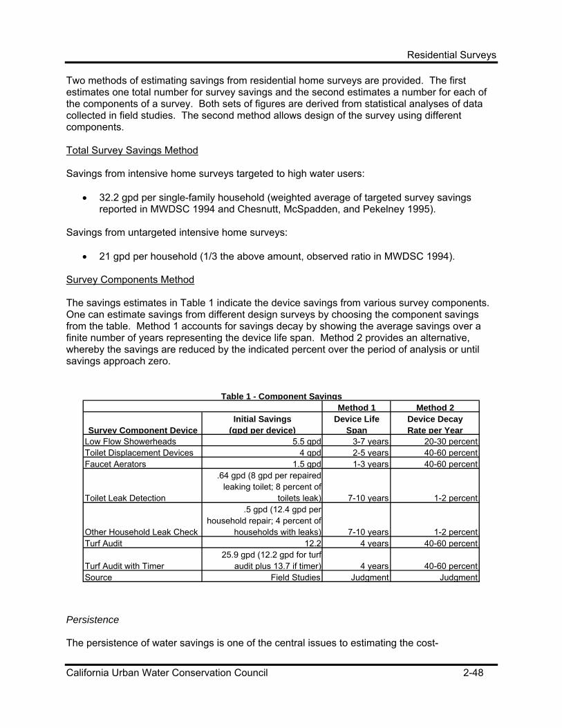
Residential Surveys
California Urban Water Conservation Council 2-48
Two methods of estimating savings from residential home surveys are provided. The first estimates one total number for survey savings and the second estimates a number for each of the components of a survey. Both sets of figures are derived from statistical analyses of data collected in field studies. The second method allows design of the survey using different components. Total Survey Savings Method Savings from intensive home surveys targeted to high water users:
• 32.2 gpd per single-family household (weighted average of targeted survey savings reported in MWDSC 1994 and Chesnutt, McSpadden, and Pekelney 1995).
Savings from untargeted intensive home surveys:
• 21 gpd per household (1/3 the above amount, observed ratio in MWDSC 1994). Survey Components Method The savings estimates in Table 1 indicate the device savings from various survey components. One can estimate savings from different design surveys by choosing the component savings from the table. Method 1 accounts for savings decay by showing the average savings over a finite number of years representing the device life span. Method 2 provides an alternative, whereby the savings are reduced by the indicated percent over the period of analysis or until savings approach zero.
Persistence The persistence of water savings is one of the central issues to estimating the cost-
Method 1 Method 2
Survey Component DeviceInitial Savings
(gpd per device)Device Life
SpanDevice DecayRate per Year
Low Flow Showerheads 5.5 gpd 3-7 years 20-30 percentToilet Displacement Devices 4 gpd 2-5 years 40-60 percentFaucet Aerators 1.5 gpd 1-3 years 40-60 percent
Toilet Leak Detection
.64 gpd (8 gpd per repaired leaking toilet; 8 percent of
toilets leak) 7-10 years 1-2 percent
Other Household Leak Check
.5 gpd (12.4 gpd per household repair; 4 percent of
households with leaks) 7-10 years 1-2 percentTurf Audit 12.2 4 years 40-60 percent
Turf Audit with Timer25.9 gpd (12.2 gpd for turf
audit plus 13.7 if timer) 4 years 40-60 percentSource Field Studies Judgment Judgment
Table 1 - Component Savings

Residential Surveys
California Urban Water Conservation Council 2-49
effectiveness of residential home surveys. This issue is rarely addressed in empirical impact evaluations because of the expense and intrinsic difficulty of providing a multiple-year measure of impact. One such example was based on data from a field study in Los Angeles (Chesnutt, McSpadden, and Pekelney 1995). Examining early participants and four years of post-intervention water use data, Figure 1 was developed. Figure 1 plots the average annual net water savings for each year following the initial home survey. The net water savings held up surprisingly well during the first three years. The fourth year appears to give some evidence of a decline in water savings, but some caveats are in order. First, there is a greater amount of uncertainty surrounding the savings in the fourth year. This is due to the smaller sample size of Phase I participants that possessed four years of post-intervention water use. The broader bands of uncertainty surrounding the fourth year of water use make it more difficult to discern any decline in water savings. Second, the estimated level of water savings in the fourth year may also reflect characteristics of the smaller sample of early participants that does not reflect later participants. The authors caution against drawing too much inference about the magnitude of decay in water savings from this early evidence and recommend more long-term follow-up of conservation program results.
The CCWD study calculated water savings persistence in three time periods subsequent to audit implementation: “Savings over the first year, second year, and beyond average 17 percent, 16 percent, and 13 percent respectively” (CCWD 1994).
0
5
10
15
20
25
30
35
40
Con
serv
atio
n (g
al. p
er H
H p
er d
ay)
1 2 3 4
Figure 1 - Years after Home Survey

Residential Surveys
California Urban Water Conservation Council 2-50
Limitations The persistence of water savings from residential surveys remains a difficult quantity to predict. Confidence in Estimates Low. 2.8.4 Program and Device/Activity Cost Estimates Program Costs Participant program costs may include:
• Cost of survey devices/materials if not fully subsidized • Installation cost if not fully subsidized
Supplier program costs may include:
• Staff time to develop survey materials, target sites, and conduct survey (if not contracted out)
• Survey equipment and devices • Administration • Contractors • Marketing
CCWD (1994) estimated their program costs as they were incurred in their 1993 CCWD program implementation (Table 2).
Action Hours CostsLabor
Audit 1.25@ $15.43/Hour $19.28Administrative Costs 5.86$ Labor Subtotal 25.14$
EquipmentShowerhead 0.61@ $2.49 1.52$ Toilet dam 1.54@ $1.20 1.85$ Bucket (1993 only) 1.80$ Faucet aerator 1.19$ Information material 3.50$ Hose nozzel 0.99$ Milage 17 mi.@ $.28/mi. 4.76$ Equipment Subtotal 15.61$
Total 40.75$ Reproduced from CCWD 1994.
Table 2 - Cost of Residential Audit

Residential Surveys
California Urban Water Conservation Council 2-51
The following are professional judgments of costs by conservation program coordinators and managers, as reported in MWDSC (1995):
• Survey, targeted indoor/outdoor: $200 • Survey, untargeted indoor: $40 • Low flow showerheads, kit: $2 • Moisture sensor, residential: $125 • Irrigation timer, residential: $230 • Swimming pool/spa covers: $5-150 • Low flow showerheads, direct install: $10-15
Plumbing retrofit costs are estimated in HUD (2002) as follows: “Device or material costs were obtained from large manufacturers/providers throughout the United States. Labor costs were assumed at $36 per hour for a laborer and $60 per hour for a technician or a plumber. The times required to complete the various tasks were approximated from literature on the subject and/or information from professionals in the field.” Additional estimated costs are listed in Table 3.
Table 3 – Estimated Costs of Implementation for Retrofit Strategies Install low-flow faucet aerators $2 Install low-flow showerheads $5-$17 Install toilet displacement devices $1 Install quick-closing flappers in toilets $14-$22 Adjust water level in toilets $20-$32 Detect and repair toilet leaks $11-29 Detect and repair faucet leaks $6 Detect and repair showerhead leaks $6-$10 Install free aerators, showerheads, toilet inserts
$12 installation cost per set for each apartment unit
Source: Reproduced plumbing retrofit costs from HUD (2002) Limitations Costs vary with scale of the program and the weather—hot and dry periods make for easier marketing to many residential customers. Confidence in Estimates Low-Medium. Achieved conservation from residential home water surveys can vary widely depending upon: (1) the content of the survey, (2) the targeted marketing, and (3) the water and wastewater rate structures in place. 2.8.5 Water Savings Calculation Formula(s) Calculations Water Savings = Survey_Savings * Number_of_Surveys

Residential Surveys
California Urban Water Conservation Council 2-52
Factors to Consider in Applying the Formula Survey savings can vary greatly depending on weather, water rates, and follow-up. Multiplying by “Number_of_Surveys” as shown above allows the calculation of program savings, not just from a single survey, assuming constant savings by scale. Survey_Savings is an average over the years of estimation, with decay imbedded. Example Calculation Water Savings = Survey_Savings * Number_of_Surveys 11,000 gpd per 1000 Surveys = (5.5gpd + 4gpd + 1.5gpd) * 1000 Surveys 2.8.6 Questions to Ask
• Are there other agencies that you can develop partnerships with to make your program more cost effective?
• Does your agency have access to grant or other partnership type funding? • Is the survey targeted, and to whom? • What marketing technique(s) will be used to enlist customer participation and will the
selected technique(s) include incentives? • How many times are customers contacted? • What are climatic conditions, and do you have the ETo for determining the right
application of water? • Are the landscape areas generally small or large, are most watered by hand or by
automatic sprinkler system? • Do you intend to conduct the surveys with agency personnel or contract out? • Does your agency allow your personnel or contractor to enter the customer’s home? • What are the elements of the survey (devices, actions, etc.)? • Do you have estimated or comparative costs for survey/device components and method
selected to implement the program? • If you intend to provide devices (BMP 2) or ULFTs (BMP 14) with your survey program,
will your personnel or the contractor install the devices and/or ULFTs. If not, how will installations be verified?
• How will you use the survey results and will results be tied to a customer specific database (customer conservation screen)?
• Are you going to design and maintain a database covering all participants and program results?
• Can you influence how the cost of this program is accounted for? If capitalized, the cost impact will be spread over “x” number of years and reduce the rate impact. If expensed, will the cost of your program have to be recovered in one year?
2.8.7 Sources CCWD (1994), “Residential Water Audit Evaluation,” prepared for Contra Costa Water District by John B. Whitcomb, Ph.D., August.

Ultra Low Flush Toilets (Residential)
California Urban Water Conservation Council 2-53
CCWD (2000), “Residential Water Survey Evaluation,” prepared for Contra Costa Water District by John B. Whitcomb, Ph.D., May. Chesnutt, T., C. McSpadden, and D. Pekelney (1995), “What is the Reliable Yield from Residential Home Water Survey Programs?” presented at the AWWA Conference in Anaheim CA, June. HUD (2002), “Retrofitting Apartment Buildings to Conserve Water,” prepared for U.S. Department of Housing and Urban Development by Water Resources Engineering Inc., May. MWDSC (1994), “Residential Water Audit Program: Evaluation of Program Outcomes and Water Savings,” prepared for Metropolitan Water District of Southern California by A&N Technical Services, Inc., December. MWDSC (1995), “Reference Document: Program Design Tool and Savings Estimates,” prepared for Metropolitan Water District of Southern California by A&N Technical Services, Inc.

Ultra Low Flush Toilets (Residential)
California Urban Water Conservation Council 2-54
2.9 Ultra Low Flush Toilets (Residential) 2.9.1 Device/Activity Description “Ultra-low-flush” (ULF) toilets are low-water-using toilets. Specifically, ULF toilets must use no more than 1.6 gallons per flush. ULF toilets employ gravity fed technology optimized for 1.6 gpf, pressure assist technology, and tip-bucket technology—the latest design introduced to the market. “High-efficiency” toilets (HET) are defined as those with flush volumes 1.3 gpf or better (Koeller 2004). HETs currently employ dual-flush and pressure-assist technologies. 2.9.2 Applicable BMPs
• BMP 1 – Residential Water Surveys. Complete residential surveys may result in ULFT replacement.
• BMP 2 – Residential Plumbing Retrofit. Concerns toilet retrofit devices rather that ULFT replacements.
• BMP 13 – Wholesale Agency Assistance. ULFT replacements are applicable to wholesale assistance and incentive programs.
• BMP 14 – Residential ULFT Replacement. Fully applicable for the residential sector. 2.9.3 Available Water Savings Estimates Summary of Individual Studies The most rigorous ULF toilet savings estimates to date are based on a series of field studies that examined the change in metered water consumption of more than 23,000 residential households and customers in Los Angeles, San Diego, and Santa Monica. Based on these field studies we present a primary method for estimating ULF toilet savings that adjusts the per toilet saving estimate for household density--number persons per household. Separate extrapolation equations are provided for both single family and multiple family sectors. Statistical models were estimated from the field study data to examine the relationship between savings and household density. Also presented is a secondary method for estimating toilet savings based upon the number of first, second, and third toilets replaced. One of the findings from field studies was the declining marginal effectiveness of ULF toilets--two toilets do not save twice as much as one toilet. When information on the number of replaced toilets per household is available to conservation planners, this secondary method can yield more accurate estimates of ULF toilet conservation potential. Per capita extrapolation assumes that the number of persons per household among participants is precisely equal to that of the service area in question. This relationship may not hold true depending upon how the ULF toilet programs are marketed. For example, many of the single-

Ultra Low Flush Toilets (Residential)
California Urban Water Conservation Council 2-55
family toilet rebate program participants exhibit, on average, a lower household density than the service area average. Several possible explanations for the difficulty of reaching high-density households exist. Because density and income are inversely related, low-income households may face tighter cash flow constraints. Conservation planners should give careful thought to the assumption of persons per household that drives per capita estimates of ULF toilet water conservation potential. The number of persons per dwelling is often used as the primary adjustment factor in mechanical estimates of conservation potential. To illustrate, consider an often-used reduction factor of 15.6 gpcd (gallons per capita per day).8 A short list of the most important problems with this method to estimate savings for ULF toilets includes:9
(1) It assumes a constant per capita effect for both single family and multiple family households. There are many reasons why multiple family savings should differ from that experienced by the single-family sector. Existing multiple family toilets tend to be older, less well maintained, and less likely to be retrofitted with a toilet displacement device. Further, one cannot rule out the possibility of fundamental differences in toilet use habits. In sum, an equivalence in ULF toilet saving potential would be far more surprising than any differences10.
(2) It assumes strict linearity in savings. The assumption of perfect proportionality (four
persons save four times as much as one) also runs afoul of findings from field studies. The water savings per household do not increase in a one-to-one relationship with the number of inhabitants. As documented in A&N Technical Services (1992a, Appendix B) functions were estimated from field data to fit observed conservation from ULF toilet replacement. Separate functions were estimated for single-family households and for multiple family households. Both functions tested for and rejected the hypothesis of a linear per capita effect at high levels of confidence. The estimated functions were referred to as conservation “mappings” because they map from household characteristics (persons per household and ULF toilets replaced per household) to expected household water savings.
(3) It provides no guidance for situations of less than complete ULF toilet replacement.
(4) It requires knowledge of the number of persons per household.
Field studies show that the first two assumptions do not exist in real world conservation programs. Problem 1 can be addressed by separately estimating extrapolation equations for
8This is based on 4 flushes per day and 3.9 gallons per flush savings. The source is Brown and Caldwell, Residential Water Conservation Projects, Summary Report, U.S. Department of Housing and Urban Development, June 1984, also known as the HUD Study. This was an important early empirical study of residential water conservation. Its quick adoption and wide use for extrapolation in the water industry attests to its ground-breaking nature. We cite the report both because it is widely used and because extrapolations citing the report are often poorly implemented. 9Additional problems not addressed here are more technical in nature. Even if the functional form were accurate, a gpcd extrapolation yields a biased estimate and produces no estimate of uncertainty. Both of these issues are documented in A&N Technical Services (1992c) pp. 12-13. 10The oft-cited HUD Study (op. cit.) only includes single-family households and therefore cannot offer any empirical weight to bear on questions of multiple family water savings differences.

Ultra Low Flush Toilets (Residential)
California Urban Water Conservation Council 2-56
single family and multiple family sectors. Problem 2 can be addressed by permitting the estimated equation to take on a nonlinear form. The primary method of estimating expected savings involves estimation of separate single family and multiple family equations (see below). Aquacraft (1999) found the “net savings” between homes with only ULF toilets and all other homes was 10 gallons per capita per day. Water consumption for toilets at the ULF toilet only homes was 24.1 gallons per household per day. Water consumption for toilets at all other homes was 47.2 gallons per household per day. Stratus Consulting (2002) estimates free riders in four service territories that include rebate, voucher, and free installation programs. Free riders are defined as “program participants who would have replaced their toilets within 12 months of the time they did even if the program did not exist.” The results show free riders from the rebate programs of Contra Costa Water District, and Municipal Water District of Southern California to be 60.1% and 62.5% respectively. Free riders attribute for 44.9% for the voucher program by the San Diego County Water Authority, and 31.7% for the free distribution program by the Los Angeles Department of Water and Power. Important caveats: This study estimates free ridership only for mature toilet replacement programs, and as such, the results are not directly applicable to programs at start-up or in their early stages. Also, the degree of free ridership depends on program design. Niagara (2003) states that their “Flapperless” tip-bucket toilet “uses 54% less water than a common 3.5 gallon toilet.” Canada Mortgage and Housing Corporation (2001) report that 50 percent of 6-liter toilets tested had a flow rate greater than 6 liters. NAHB (2002) report the results of performance testing of ULF toilet fixtures. The study shows that there is an important difference in the performance characteristics between various toilet models. Further, replacement of flapper valves with generic flappers not particularly designed for the toilet in question resulted in flow rates of 1.03 to 4.66 gpf. Of the 33 models tested with the generic flapper, 28 used more than 1.6 gpf, with an average of 2.91gpf. A&N Technical Services (2001) found savings of 21.8 gallons per day per toilet replacement on the Monterey Peninsula, corresponding to a 10.6 percent reduction in total water consumption among participants. Veritec Consulting and J. Koeller (2003, 2004) report the results of performance testing of a wide range of ULF toilets. Of the 44 “off the shelf” toilet models tested, only 24 met the 250 gram performance benchmark. Of the 24, 11 met a 500 gram test.
Dual-Flush and Flapperless Toilets Koeller (2003) summarizes flush-volume results from five recent studies that included dual-flush toilets. Table 1 shows flush volumes for inefficient toilets measured before replacement and the new dual-flush toilets under study. Note that flush volume comparisons cannot be directly translated into expected net water savings. Canada Mortgage and Housing Corporation (2002, first source in Table 1) reports that dual-flush toilets reduced consumption by 23 to 32 percent more than 6-liter toilets.

Ultra Low Flush Toilets (Residential)
California Urban Water Conservation Council 2-57
Aquacraft (2000) found that the ULF toilets that were installed, which included some dual-flush toilets, saved an average of 10.9 gcd. The dual-flush installations saved 24 percent more than the 1.6 ULF toilets. Double-flush frequency differences were not statistically significant for either the before / after or the ULF toilets / dual flush comparisons. Aquacraft (2003) found flush volumes for the Niagara Flapperless toilet to be 1.7 gpf with 9 gallons per capita per day. The Caroma dual-flush averaged 1.34 gpf with 9.9 gallons per capita per day—higher than the Flapperless due to a higher number of flushes. PNNL (2001) also reports toilet savings of 2.6 gpf, representing a 67 percent savings, and that toilet savings are the largest category of savings among all, which included clothes washers, dishwashers, showerheads, and aerators. Aquacraft (2004) found flush volumes for the Niagara Flapperless toilet to be 1.57 gpf with a standard deviation of .14. Jordan Valley (2003) and Mohadjer (2004) report results from a study of 275 toilets including dual-flush, flapperless, and conventional ULF toilets. The study found 21.8 gallons per day savings from the Niagara Flapperless toilet, and 26.8 gallons per day from the Caroma dual-flush. The Gerber ULF toilet saved 19.8 gallons per day. These figures represent the savings only from lower flush volume. The study separately identified savings from eliminating leaks in the old toilets: 46 percent of the total savings can be attributed to leak repair—an average of 19.3 gpd. Persistence At least one field study tested for, and could not detect, any downward trend in the level of water savings amongst early participants in ULF toilet programs in Los Angeles and Santa Monica. It had been hypothesized that much of the water savings initially observed from ULF toilet replacement came from the removal of previously leaking toilets. If this were the case, one might expect to see a distinct decline in the level of water savings over time; as ULF toilets age, they too would eventually become as leaky as the toilets replaced. Results from the first three years of ULF toilet programs cannot discern any such downward trend in water savings. Data from single-family survey programs in Los Angeles and San Diego also suggest that the magnitude of leaking toilet problem may be overstated. Leakage rates among toilets tested were 4-5.6 percent among participants in the City of San Diego Water Conservation residential surveys and 7 percent among participants in the City of Los Angeles Home Survey Program.
Table 1 – Flow Volume for Dual-Flush Toilets Study Inefficient Toilet Volume Dual-Flush Volume
Veritec Consulting/CMHC (2002) 3.72 gpf 1.11 gpf Aquacraft/Seattle (2000) 3.61 gpf 1.25 gpf Aquacraft/Oakland (2003) 3.88 gpf 1.34 gpf PNNL/Oregon (2001) 3.9 gpf 1.3 gpf Jordan Valley, Utah (2003) 4.16 gpf 1.20 gpf Source: Primary sources summarized in Koeller (2003).

Ultra Low Flush Toilets (Residential)
California Urban Water Conservation Council 2-58
Another hypothesis for savings decay is that background saturation levels of ULFTs are increasing, cutting into incremental savings. University of Arizona (2000) report in their follow up of aging low consumption toilets that the actual flow rate was on average 24 percent higher than the 1.6 gpf design rating, as well as a somewhat higher rate of flapper leaks and double flushing. California Urban Water Conservation Council (2004) reports results of a study of toilet flappers in the field that contributes to the understanding of toilet savings persistence. In testing of toilets installed between 1992 and 2002, less than 6 percent of the toilets were leaking through the flapper valve. The study did not find a correlation between leakage and the age of the toilet. Of the 205 customers who used in-tank toilet bowl cleaners only 17 had leaky flappers. Of all the toilets inspected, nearly 90 percent had their original flapper. Limitations The study of savings persistence has not received enough attention in field research over the years. However, this is changing in important ways. For example, the recent research on flapper valves contains important evidence of effectiveness over time related to ULFT savings persistence (CUWCC 2004). Another limitation of existing research is that savings results depend importantly on the make and model of toilet. CMHC (2004) demonstrates the large differences in the performance of popular model ULF toilets. Confidence in the Estimates High. These estimates are based on rigorous field studies. 2.9.4 Program and Device/Activity Cost Estimates Program Costs Participant program costs may include:
• Cost of ULF toilet and installation not reimbursed by rebate
Supplier program costs may include:
• Staff time to administer rebate program • Rebate incentive • Administration • Contractors • Marketing
Current retail prices of residential-grade two-piece standard-style ULF toilets that are reported to work well range from $189 to $300 (e.g., American Standard 2005 and Love Plumbing 2005). Free distribution program costs for fixtures are wholesale rates for bulk purchases, the cost of service for distribution, and other costs for planning and coordination. For example, the City of

Ultra Low Flush Toilets (Residential)
California Urban Water Conservation Council 2-59
Long Beach budgeted $384,000 for 4,000 ULF toilets for distribution and a $150,000 fee for one year for a contractor to distribute the toilets (including 1,000 rebates in addition to the 4,000 toilets distributed), $17,700 for the program coordinator’s salary and fringe benefits, and $30,000 for other direct costs such as planning and maintenance (Long Beach 2001). Although the following dollar figures regarding the BAYSAVER Program are not the most recent, they provide considerable detail regarding complete program costs from multiple perspectives of analysis. City of Santa Monica planning documents for their BAYSAVER Phase I and II Programs estimate cost of ULF toilets in different sectors (Santa Monica 1989 and 1992). A&N Technical Services (1995) also examine the cost of ULF toilets in its study of toilet savings. As demonstrated in the CUWCC Cost-Effectiveness Guidelines, these figures can be used to show that costs vary not only by sector but by delivery mechanism—rebate or direct install programs. The ULFT Study reports retail toilet purchase costs of $130 and the BAYSAVER Phase II Proposal reports that ULF toilet prices are falling and are available for as low as $100. Bulk purchases were made at approximately $60 per toilet. The purchase cost estimate comes from the direct installation program in the City of Santa Monica. A key determinant of cost of the BAYSAVER Program is the delivery mechanism for the ULF toilets. About half of the single family ULF toilets are delivered with the “rebate” option and half are directly installed. In contrast, the majority of multi-family and commercial ULF toilets are directly installed. With the rebate, the participant purchases ULF toilet at retail and installs the toilet, after which the City provides a rebate check ($75 in BAYSAVER Phase II). With direct installation, the City purchases the ULF toilets in bulk at wholesale and installs the toilet and the customer provides a co-payment ($35 in BAYSAVER Phase II). Although single-family installation costs are approximately $70, they are considerably less when negotiated in large numbers by the City for direct installation and for multiple family sites where economies of scale become apparent ($50 and $40 respectively). Other costs of the program include rebate processing, advertising, and workshops. With the rebate program, from the customer perspective, costs include the acceleration in toilet replacement costs, including installation, less the rebate. Table 2 shows the costs to replace an existing toilet, with direct installation, costs include only the $35 co-payment—again, this should be the acceleration in costs. From the total society perspective, costs include the acceleration in the costs of the toilet, its installation, and other costs. From the supplier perspective, costs include the direct installation program including the toilet, its installation, and other costs, less the customer co-payment. Since many participants install toilets themselves rather than hiring a plumber, their costs would not include the installation cost shown in Table 2.
SectorToilet Cost
[1]Installation
[2]Rebate
[3]
Other Costs
[4]
Participant Costs
[5]
Supplier Costs
[6]
Total Society
Costs [7]Single Family Rebate $120 $70 $75 $40 $115 $115 $230Single Family Direct $60 $65 $40 $35 $130 $165Multi-Family Direct $60 $55 $40 $35 $120 $155Source: CUWCC GuidelinesAll costs are dollars per ULF toilet[4] “Other Costs” includes contract inspections and processing, advertising, workshops, and toilet recycling.[5] = [1]+[2] - [3] for Rebate and $35 Copayment for Direct Installation [6] = [3]+[4] for Rebate and [1]+[2]+[4] - [3] for Direct Installation[7] = [1]+[2]+[4]
Table 2 - Program Costs ($/ULFT)

Ultra Low Flush Toilets (Residential)
California Urban Water Conservation Council 2-60
Dual-Flush and Flapperless Toilets Canada Mortgage and Housing Corporation (2002) reports the costs of the toilets used for their dual-flush study were “approximately Can$160 for the Aris 6-litre, Can$170 for the Flapperless 6-litre, Can$300 for the Drake, Can$300 for the Tasman dual-flush and Can$400 for the Caravelle dual-flush.” Limitations Costs depend on program design. All programs, including rebate programs and direct installation, need to be clearly defined. Cost estimates should be viewed in light of the time that has elapsed since the above figures were reported and with respect to the scale of the program under consideration (volume purchases). Finally, some of the early toilet replacement programs faced the problem that installed ULFTs did not work well and suppliers faced unforeseen costs of replacements. Confidence in Estimates Medium. 2.9.5 Water Savings Calculation Formula(s) Calculations Savings Calculation Primary Method: Toilet Savings Adjusted for Household Density These equations assume that only household density information is available and savings estimates are desired on a per ULF toilet basis. (If information on both persons per household and toilets per household were available, the conservation mappings could be directly used to produce predicted household water saving. See Appendix B of A&N Technical Services 1992a). The resulting prediction of conservation from ULF toilets forms the dependent variable for the extrapolation equations. Estimates of the parameters of the equations are obtained through the following regression models: SSF = 6.693 * Persons_Dwelling - 0.529 * (Persons_Dwelling)2 + 7.826 SMF = 19.138 * Persons_Unit - 0.942 * (Persons_Unit)2 + 2.181 Savings Calculation Secondary Method: Toilet Savings Adjusting for Completeness of Retrofit The primary method of estimating toilet savings does not address Problems 3 (Less than Complete ULFT Replacement) and 4 (Number of Persons per Household). The secondary method addresses both problems--it corrects for the declining marginal effectiveness of ULF toilet replacements and requires no knowledge of the expected household density among program participants. It only requires knowledge of number of toilets replaced per household. SSF = 29.9 * Number of First Toilets Replaced + 20.6 * Number of Second Toilets Replaced + 19.1 * Number of (Third or higher) Toilets Replaced

Ultra Low Flush Toilets (Residential)
California Urban Water Conservation Council 2-61
SMF = 44 * Number of First Toilets Replaced + 34 * Number of Additional Toilets Replaced Source: A&N Technical Services (1995) Table III-3 and III-4. Factors to Consider in Applying the Formula Additional secondary adjustments can also be made. Information on the distribution of 3.5 gallon per flush and 5 to 7 gallon per flush toilets can be incorporated using methods documented in the CUWCC Memorandum of Understanding, Exhibit 6, Section II, amended March 9, 1994. Few conservation planners, however, have access to accurate information on the mix of pre-existing toilets. Example Calculation Table 3 shows results from calculations of water savings for three hypothetical suppliers with different housing density. The calculations are based on the primary savings calculation method described above. Examples of the complete cost-benefit analysis and cost-effectiveness analysis are illustrated in the CEA Guidelines, Chapter 4.
Table 3 - Residential ULFT Savings Sample Calculation
Supplier Yr
Single Family Persons per Household
Multi- Family Persons per Household
Single Family Savings
gpd/ULFT
Multi-Family Savings
gpd/ULFT Supplier A 1995 2.50 2.00 21.2 36.7Supplier B 1995 3.50 3.00 24.8 51.1Supplier C 1995 4.50 4.00 27.2 63.7 2.9.6 Questions to Ask
• What is the age of the housing stock in the relevant service area (pre or post code), and is the housing stock of such an age and type that drain lines will provide adequate flow for 1.6 (or 1.0) gpf toilets?
• Are there other agencies that you can partner with to make your program more cost effective?
• Does your agency have access to grant or other partnership type funding? • Is the program targeted, and to which sector (SF, MF, low income, other) • Is your water service area metered or un-metered? (Marketing and incentives will
definitely vary based on your response to this question.) • Will your program be a free distribution; co-pay (customer and agency share in the cost);
direct install (when use, often limited to low income and elderly); or rebate? • Will your program be conducted using agency personnel or contracted out? • Will your agency limit the approved models to those toilets that have been tested for long
term water savings and customer satisfaction? • Are installations verified? • Will results be tied to a customer specific database (customer conservation screen)?

Ultra Low Flush Toilets (Residential)
California Urban Water Conservation Council 2-62
• Are you going to design and maintain a database covering all participants and program results?
• Is this program in combination with other measures (showerheads, surveys, public education, price changes)?
• Can you influence how the cost of this program is accounted for? If capitalized, the cost impact will be spread over “x” number of years and reduce the rate impact. If expensed, the cost of your program will have to be recovered in one year?
• When applying an existing savings estimate, how similar is the service area in terms of socioeconomic characteristics and conditions?
2.9.7 Sources A&N Technical Services (1992a) Chesnutt, T.W., Bamezai, A., and C.N. McSpadden, The Conserving Effect of Ultra Low Flush Toilet Rebate Programs. A report for the Metropolitan Water District of Southern California, June 1992. A&N Technical Services (1992b) Chesnutt, T.W., Bamezai, A., and C.N. McSpadden, Continuous-Time Error Components Models of Residential Water Demand, A report for the Metropolitan Water District of Southern California, June. A&N Technical Services (1992c) Chesnutt, T.W., Bamezai, A., and C.N. McSpadden, Mapping the Conserving Effect of Ultra Low Flush Toilets: Implications For Planning, A report for the Metropolitan Water District of Southern California, June. A&N Technical Services (1994a) Bamezai, A. and T.W. Chesnutt, Public Facilities Toilet Retrofits: Evaluation of Program Outcomes and Water Savings, A report for the Metropolitan Water District of Southern California, December. A&N Technical Services (1994b) Bamezai, A. and T.W. Chesnutt, Residential Water Audit Program: Evaluation of Program Outcomes and Water Savings, A report for the Metropolitan Water District of Southern California, December 1994. A&N Technical Services (1995) Chesnutt, T.W., C.N. McSpadden, and A. Bamezai, Ultra Low Flush Toilet Programs: Evaluation of Program Outcomes and Water Savings, A report for the Metropolitan Water District of Southern California, July. A&N Technical Services, Inc., “Statistical Analysis of ULF Toilet Replacement on the Monterey Peninsula,” for Monterey Peninsula Water Management District, Draft Final, February 2001. American Standard (2005), Direct sales prices reported at URL: www.americanstandard-us.com. Aquacraft, Inc., “Residential End Uses of Water,” prepared for American Water Works Research Foundation, 1999. Aquacraft, Inc., “Seattle Home Water Conservation Study,” prepared for Seattle Public Utilities and the U.S. EPA, December 2000.

Ultra Low Flush Toilets (Residential)
California Urban Water Conservation Council 2-63
Aquacraft, Inc., “Residential Indoor Water Conservation Study,” prepared for the East Bay Municipal Utilities District and the U.S. EPA, July 2003. Aquacraft, Inc., “Tampa Water Department Residential Water Conservation Study,” January 2004, prepared for Tampa Water Department and the U.S. EPA. Brown and Caldwell (1984) “The HUD Study,” Residential Water Conservation Projects, Summary Report, U.S. Department of Housing and Urban Development, June. California Urban Water Conservation Council, “Toilet Flapper Study: Final Report,” prepared by Koeller and Company, December 2004. CUWCC (2004), “High Efficiency Toilets,” prepared by J. Koeller for the California Urban Water Conservation Council, revised October. Canada Mortgage and Housing Corporation (CMHC), “Dual-Flush Toilet Testing, 2001,” Research Highlights, Ottawa, September 2002. Canada Mortgage and Housing Corporation (CMHC), “Maximum Performance Testing of Popular Water-Efficient Toilet Models,” Research Highlights, Ottawa, May 2004. Canada Mortgage and Housing Corporation, “Independent Toilet Testing Program, 2001,” Research Highlights, Ottawa, December 2001. Canada Mortgage and Housing Corporation, “Six-Litre Toilet Performance Monitoring Program, 2001,” Research Highlights, Ottawa, 2001. Caroma USA Inc., “Caroma Quick Facts,” URL: www.caromausa.com downloaded April 2004. Chesnutt, T.W., Moynahan, M., and A. Bamezai (1992), Ultra-Low-Flush Toilet Rebate Programs in Southern California: Lessons For Water Managers and Planners, Proceedings of the American Water Works Association Conference in Vancouver, Canada, June. Jordan Valley Water Conservancy District, “Residential Ultra Low Flush Toilet Replacement Program,” Undated, file created in 2003. Koeller, J., “Dual-Flush Toilet Fixtures—Field Studies and Water Savings,” December 2003. Long Beach Water Department, “Water Ambassador and Ultra Low Flush Toilet Programs,” Proposal in response to CALFED/California Department Of Water Resources Water Use Efficiency Program Proposal Solicitation, February 2001. Love Plumbing and Remodel, URL: www.terrylove.com, April 2005. Mohadjer, P., “Water Savings of an Ultra Low Flush Toilet Replacement Program,” Proceedings of Water Sources Conference, American Water Works Association, 2004. NAHB Research Center, “Water Closet Performance Testing,” prepared for Seattle Public Utilities and East Bay Municipal Utility District, September 2002.

Ultra Low Flush Toilets (Residential)
California Urban Water Conservation Council 2-64
Niagara Flapperless Inc, “Introducing Tipping Bucket Technology,” URL: www.flapperless.com downloaded June 2003. Pacific Northwest National Laboratory, “The Save Water and Energy Education Program: SWEEP: Water and Energy Savings Evaluation,” prepared for the U.S. Department of Energy, May 2001. Santa Monica (1989), “Recommendation to Approve the Residential Plumbing Fixture Rebate Program,” Proposal to the Mayor and City Council from City Staff, City of Santa Monica, July 25. Santa Monica (1992), “Recommendation to Approve Phase II of the BAYSAVER Plumbing Fixture Rebate Program,” Proposal to the Mayor and City Council from City Staff, City of Santa Monica, February 11. Sloan Flushmate Division, “Technical Update,” URL: www.flushmate.com, 2002. Stratus Consulting Inc., “Freeriders in ULFT Programs,” for the California Urban Water Conservation Council December 2002. Veritec Consulting and J. Koeller, “Maximum Performance Testing of Popular Toilet Models,” Koeller and Company December 2003. Veritec Consulting and J. Koeller, “Maximum Performance Testing of Popular Toilet Models: May 2004 Update #1,” Koeller and Company May 2004. Water Resources Research Center at the University of Arizona, “Functioning of Aging Low-Consumption Toilets in Tucson: A Follow-Up With Rebate Program Participants,” prepared for the City of Phoenix and the U.S. Bureau of Reclamation, October 2000.

CII Surveys
California Urban Water Conservation Council 2-65
2.10 CII Surveys: Cooling and Industrial Processes 2.10.1 Device/Activity Description Commercial, Institutional, and Industrial (CII) surveys can range from short “walkthroughs” to sophisticated water efficiency studies. Customers are targeted with a marketing strategy and incentives. Recommendations are made to reduce water consumption at the facility. The recommended actions may then be implemented by the site managers. One challenge is understanding the actual water savings that results from surveys; most of the published literature estimates saving from recommended conservation measures, but not the actual savings determined in a follow-up study. One cannot underemphasize the need to distinguish between savings potential and actual savings when reading the CII survey literature. Recommended measures include sanitation, irrigation, kitchen, industrial, cooling, laundry, wastewater, and others. Savings and cost data for faucets, urinals, ULF toilets, and landscape irrigation are examined in other sections of this document. This section focuses on cooling towers and industrial process savings. Two broad categories of water loss in cooling towers include bleed-off (draining cooling water) and uncontrolled losses (drift loss from mist and leaks). In some parts of California nearly all cooling towers are re-circulating systems (as opposed to single pass systems) and many of these have conductivity controllers to automatically manage total dissolved solids by adjusting bleed-off and make-up. Water savings potential for multi-pass systems are related to (1) better tuned conductivity controllers and (2) adding conductivity controllers if not present. Industrial process savings is a large category of potential savings, but is as diverse in nature as the industrial base. Industrial processes may include: metal plating, electronics fabrication, photographic processing, product water and rinses, in-plant cleaning, sterilizers, container cleaning, kitchens and water treatment and regeneration. 2.10.2 Applicable BMPs BMP 9 – Conservation Programs for Commercial, Industrial, and Institutional Accounts. Implementation of this BMP includes:
a) identifying and ranking CII customers according to use, b) establishing targets for ULFT replacements in the CII sector, and EITHER c) implementing water-use surveys and incentives to 10 percent of CII customers within 10
years, OR d) achieving water use reductions equal to or exceeding 10 percent over 10 years.
2.10.3 Available Water Savings Estimates Summary of Individual Studies Western Policy Research (1996) has analyzed data for the Metropolitan Water District of Southern California on its CII survey program. Three types of CII surveys have been
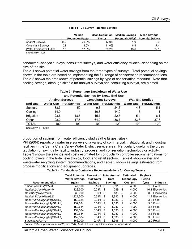
CII Surveys
California Urban Water Conservation Council 2-66
conducted--analyst surveys, consultant surveys, and water efficiency studies--depending on the size of the site. Table 1 shows potential water savings from the three types of surveys. Total potential savings shown in the table are based on implementing the full range of conservation recommendations. Table 2 shows the breakdown of potential savings by type of conservation measure. Note that cooling savings, although sizable for analyst surveys and consulting surveys, are a small
proportion of savings from water efficiency studies (the largest sites). PPI (2004) reports on water use surveys of a variety of commercial, institutional, and industrial facilities in the Santa Clara Valley Water District service area. Particularly useful is the cross tabulation of savings by facility, industry, process, and conservation technology or activity. Table 3 shows the savings and costs estimated for conductivity controller recommendations for cooling towers in the hotel, electronics, food, and retail sectors. Table 4 shows water and wastewater recycling system recommendations, and Table 5 shows savings estimated from process modifications and equipment upgrades.
nMedian
Reduction FactorMean Reduction
FactorMedian Savings Potential (AF/yr)
Mean Savings Potential (AF/yr)
Analyst Surveys 145 20.3% 17.9% 1.9 3.3 Consultant Surveys 22 18.0% 11.0% 8.4 7.4 Water Efficiency Studies 12 17.8% 29.2% 15.6 72.1 Source: WPR (1996)
Table 1 - CII Survey Potential Savings
End Use Water Use Pot.Savings Water Use Pot.Savings Water Use Pot.SavingsSanitary 33.3 50 9.3 24.6 4.8 5.1Cooling 14.9 14 10.8 14.2 6 1Irrigation 23.6 18.5 15.7 22.5 5.4 6.1Other 28.2 17.5 64.2 38.7 83.8 87.8TOTAL 100 100 100 100 100 100Source: WPR (1996)
Wat. Eff. StudiesConsultant SurveysAnalyst Surveys
Table 2 - Percentage Breakdown of Water Use and Potential Savings By Broad End Use
Recommendation
Total Potential Water Savings
(gals)
Percent of Total Water
Savings
Total Annual Cost
Savings
Estimated Technology
Cost ($)
Payback Period (yrs) Industry
EmbassySuites(CR=3) 547,000 0.15% 2,091$ 4,000$ 1.9 HotelMaxim#1(CycleRate=4) 122,500 0.03% 249$ 4,000$ 16.1 ElectronicsMaxim#2(CycleRate4) 238,000 0.06% 483$ 4,000$ 8.3 ElectronicsMaxim#3(CycleRate2.5) 1,424,500 0.39% 2,892$ 4,000$ 1.4 ElectronicsMohawkPackaging#1(CR=1.1) 159,684 0.04% 1,036$ 4,000$ 3.8 FoodMohawkPackaging#2(CR=1.1) 159,684 0.04% 1,033$ 4,000$ 3.8 FoodMohawkPackaging#3(CR=1.1) 159,684 0.04% 1,033$ 4,000$ 3.8 FoodMohawkPackaging#4(CR=1.1) 159,684 0.04% 1,033$ 4,000$ 3.8 FoodMohawkPackaging#5(CR=1.1) 159,684 0.04% 1,033$ 4,000$ 3.8 FoodMohawkPackaging#6(CR=1.1) 159,684 0.04% 1,033$ 4,000$ 3.8 FoodSafeway#1(CR=3) 365,000 0.10% 1,396$ 4,000$ 2.9 RetailSource: Table reproduced from PPI, Inc. 2004, Table 3.7; industry information from Appendix B.
Table 3 - Conductivity Controllers Recommendations for Cooling Towers

CII Surveys
California Urban Water Conservation Council 2-67
Sweeten and Chaput (1997) report analyses of CII surveys at a broad range of sites, ranging from large industrial facilities to smaller commercial and institutional sites (source data for the WPR study cited above). Overall, the surveys identified a potential savings of 29 percent, 30 percent of which was reported to be implemented in follow-up telephone calls. The study further reports that large industrial sites have the greatest potential savings, but technical complexity makes achieving those savings challenging. Successful savings at large industrial facilities would be facilitated by working with performance-based contractors or manufacturer’s representatives with an interest in the efficient operation of process equipment. Ploeser, Pike, and Kobrick (1992) present estimates of use and savings potential for cooling towers for different types of CII sites. The savings programs may have included conductivity controllers, cooling water management (sulfuric acid, filtration, etc.), addition of recirculation system, or air cooling systems. The study only makes gross savings potential estimates so these conservation methods are indistinguishable from each other. Lelic and Blair (2004) reported a 21 percent decrease in cooling tower make up water as a result of variable speed drives for cooling fans. Energy savings are reported as well. Gentili (2003) reports the savings from increasing the cycles of concentration with controllers of 1,850,000 and 1,250,000 gallons per year respectively from two large cooling towers.
Company Facility
Total Potential
Water Savings
(gals)
Percent of Total Water
SavingsTotal Annual Cost Savings
Estimated Technology
Cost ($)
Payback Period (yrs) Industry
Accretech 2,800,000 0.76% 20,608$ 26,000$ 1.7 ElectronicsCAPaperboard 58,968,000 15.95% 170,000$ 230,000$ 0.6 PaperboardConAgra 52,000 0.01% 9,966$ 3,700$ 0.4 FoodKomag 26,748,000 7.23% 225,242$ 100,000$ 0.5 ElectronicsMaximIntegrated 25,762,464 6.97% 285,751$ 185,000$ 1.0 ElectronicsMohawkPackaging 520,000 0.14% 2,512$ 3,700$ 1.5 FoodNovellusBuilding81 5,493,124 1.49% 27,143$ 75,000$ 1.7 ElectronicsNovellusBuilding4000 14,000,305 3.77% 106,122$ 85,000$ 0.8 ElectronicsPrudentialOverallSupply 2,080,000 0.56% 21,525$ 65,000$ 3.0 LaundrySJValleyPlating 1,231,360 0.31% 5,430$ 45,000$ N/A Metal FinishingSmurfitStone 73,584,000 19.90% 529,453$ 750,000$ 1.4 PaperboardSmurfitStone(FelShowers) 23,652,000 6.40% 173,132$ 250,000$ 1.4 PaperboardTycoElectronics 1,558,440 0.42% 57,925$ 110,000$ 2.0 ElectronicsSource: Table reproduced from PPI, Inc. 2004, Table 3.6; industry information from Appendix B.
Table 4 - Water and Wastewater Recycling System Recommendations
Facility Recommendation
Total Potential Water Savings
(gals)
Percent of Total Water
Savings
Total Annual
Cost Savings
Estimated Technology
Cost ($)
Payback Period (yrs) Industry
CAPaperboard Dynamic Seals – Paperboard Industry 19,292,000 5.22% 77,168$ 50,000$ 1.5 PaperboardSmurfitStone Dynamic Seals – Paperboard Industry 23,652,000 6.40% 173,132$ 50,000$ 0.3 PaperboardSmurfitStone Felt Showers Spray Valves – Paperboard 18,980,000 5.10% 3,780$ Unknown 0.0 PaperboardConAgra CHP* System & Sanitary Sprayers 2,700,100 0.73% 13,042$ 20,000$ 1.5 FoodMohawkPackaging CHP* System & Sanitary Sprayers 2,700,100 0.73% 13,092$ 20,000$ 1.5 FoodSmurfit-Stone CHP* System & Sanitary Sprayers 2,920,000 0.79% 21,374$ 10,000$ 0.5 Paperboard*Central High Pressure (CHP) System & Sanitary SprayersSource: Table reproduced from PPI, Inc. 2004, Table 3.6; industry information from Appendix B.
Table 5 - Process Modifications and Equipment Upgrade Recommendations
CII Surveys
California Urban Water Conservation Council 2-68
EPA/CADWR (1997) conducted a national study that included 13 cities across the country to determine the savings potential from commercial water users. A total of 22 categories of water users were considered. Aside from toilets and landscape, water uses included laundries, kitchens, process water, and cooling towers. Average water savings potential ranged from 9 percent to 31 percent. Whitcomb (2001) provides a comprehensive overview of the requirements of BMP 9 and the implementation of programs in service thereof. Case studies are included to illustrate how to successfully design, promote, and implement CII water conservation programs. DeOreo, Gentili, and Mayer (2004) report that 2.5 AFY savings from supermarkets in Southern California can be expected from water efficiency measures. Sinclair and Phibbs (2004) report 35% savings from conservation measures at an automobile assembly plant. Smith and Yuhas (2004) report savings potential of 40% at ICI sites including offices, hotels, restaurants, community centers, churches and child care facilities. CA DWR (2004) presents a series of case studies that contain savings estimates in a variety of CII processes, including: cleaning process at an automotive paint manufacturing, boiler water blow down recovery, clothes laundry pre-treatment recycling, leak repair in the retail sector, insulation and reuse at a dairy plant, recycling, reuse, process modification at a food processing plant, repairing steam and water leaks and install low flow devices at a medical facility, clean-in-place systems at an ice cream plant, spray nozzles at an animal research facility, purification and water recovery at a bottling plant, recycling de-ionized water at an automobile plant, and reducing wash water flow at a fruit processing plant. Vickers (2001) presents a series of case studies based on referenced primary sources in the areas of water recycling in the manufacture of printed circuit boards, process washing in the manufacture of semiconductor chips and other electronic parts, salt-water air scrubbing of VOCs, metal finishing rinse water, and materials transfer such as agricultural produce fluming. In addition, this volume contains an extended exposition of the water use and conservation in cooling towers. One case study described a cooling tower that achieved 75 percent savings in makeup waster by installing a new valve and a conductivity controller. Persistence No study considering the persistence of savings from CII survey programs has been found. Limitations The savings figures reported here are potential savings based on full implementation of survey recommendations. Actual savings may be considerably different due to partial implementation or varying effectiveness. Because of CII site heterogeneity and limitations of the study sample, extrapolation of findings to CII sites outside the sample should be done with caution. Confidence in Estimates

CII Surveys
California Urban Water Conservation Council 2-69
Low when generalized outside the study sample. Future efforts should include empirical measurement of water savings considering behavior (maintenance, etc.); the interaction of multiple conservation technologies (water maintenance, filtration, etc.); the diversity of such CII sites and savings technologies; the persistence of savings, and the relationship between recommended conservation actions and those actually implemented. 2.10.4 Program and Device/Activity Cost Estimates Program Costs Participant program costs may include:
• Costs of additional water savings equipment or processes that would not have been utilized without the audit.
Supplier program costs may include:
• Staff time to audit water users and make recommendations, if not contracted out. • Administration • Contractors • Marketing
Table 6 shows the costs of full implementation of the recommendations from each of the three different types of CII surveys in the WPR study. Rebates or financial incentives are not subtracted from these figures. Table 7 shows the costs and cost-effectiveness of the surveys. Total costs are the sum of customer costs to implement the recommendations and survey costs.
Analyst SurveyConsultant
SurveyWater Efficiency
StudyAverage Survey Cost $600 $1,484 $8,121Average Potential Savings/Yr. 3.3 AF 8.4 AF 35.9 AF
100% of average potential 43$ 42$ 54$ 80% of average potential 54$ 52$ 67$ 60% of average potential 72$ 70$ 89$ 40% of average potential 108$ 105$ 134$ 20% of average potential 216$ 210$ 268$ Source: WPR (1996)
Cost of Saved Water ($/AF)
Table 7 - Cost-Effectiveness of CII Surveys
Median Cost Mean CostAnalyst Surveys 1,014$ 3,598$ Consultant Surveys 6,828$ 12,387$ Water Efficiency Studies 30,035$ 97,527$ Source: WPR (1996)
Table 6 - CII Survey Costs of Full Implementation

CII Surveys
California Urban Water Conservation Council 2-70
Lelic and Blair (2004) report the cost of a variable speed drive installation is $3,000 for hardware and parts, plus part time staff time over four days. Down time was less than 40 minutes. Gentili (2003) reports the “Installed cost for Conductivity/pH controllers is in the range of $1,700 - $4,000.” DeOreo, Gentili, and Mayer (2004) and Aquacraft (2003) report the cost of supermarket conservation programs that include water cooling and other measures is $27,000 in present value terms over the life span of the project. Limitations Program costs will vary widely depending on the industry type and survey type. Note that program costs reported here are for full implementation of survey recommendations. Confidence in the Estimates Low-Medium. 2.10.5 Water Savings Calculation Formula(s) Calculations Although CII savings are heterogeneous and one equation overly simplifies such calculations, we can generally consider savings as the product of water use, savings potential in percentage terms, and savings implementation in percentage savings terms: S = Use * SavingsPotential * ImplemenationPercentage where:
• S is savings in gpd per site from cooling towers. • Use is water consumption in gpd. • SavingsPotential is the technical potential for water savings identified by the water
survey (percent savings from pre-program use). • ImplementationPercentage is the percent of the savings potential that is implemented.
Factors to Consider in Applying the Formula This formula simple formulation is useful only to the extent that the savings estimates are applied to the appropriate sites. Example Calculation Table 8 shows calculated savings. Referring back to Table 7 shows the cost-effectiveness calculations presented in the WPR study. The calculations assumed a 6% discount rate, a five-year life span, and constant savings over time. The table shows how the cost-effectiveness

CII Surveys
California Urban Water Conservation Council 2-71
varies considerably depending on how much of the savings potential is achieved in practice, on average.
2.10.6 Questions to Ask
• Are there other agencies that you can partner with to make your program more cost effective?
• Can you now identify your CII customers by class? • What are the elements of the survey? • Will you do interior and exterior components at the same time? • Does your agency have internal expertise to perform the more involved surveys? • Does your agency have access to grant or other partnership type funding? • Will your agency offer incentives to promote implementation? • Has your agency considered utilizing the services of a “pay-for-performance” contractor? • What sub-sectors/technologies are targeted? • Are recommendations implemented and verified? • Are savings determined with engineering estimates or measured savings from field
studies? • Can you influence how the cost of this program is accounted for? If capitalized, the cost
impact will be spread over “x” number of years and reduce the rate impact. If expensed, will the cost of your program have to be recovered in one year?
• Is operator training included in implementation of the program? 2.10.7 Sources Aquacraft, Inc., “Demonstration of Water Conservation Opportunities in Urban Supermarkets,” for California Department of Water Resources/U.S. Bureau of Reclamation and CalFed Bay-Delta Program, September 2003. Black & Veatch (1991), “Summary Report,” Nonresidential Water Audit Program, prepared for the Board of Water Commissioners, Denver, CO, July. Brown and Caldwell (1990), “Case Studies of Industrial water Conservation in the San Jose Area,” City of San Jose / CA DWR, Feb.
Table 8 - Cooling Tower Savings (gpd/site)Site Total Site Total Cooling
Mean Savings Mean Savings Percent Savingsn (AF/yr) (gpd) from Cooling (gpd/site)
Analyst Surveys 145 3.3 2,944 14.0% 412Consultant Surveys 22 7.4 6,603 14.2% 938Water Efficiency Studies 12 72.1 64,332 1.0% 643Source: WPR (1996) and author's calculations.

CII Surveys
California Urban Water Conservation Council 2-72
California Department of Water Resources (CA DWR, 2004), “Water Efficiency Guide for Business Managers and Facility Engineers, ” October. California Department of Water Resources (CA DWR, 1994), “Government/Utilities/Private Industry Partnership Program, Evaluation and Recommendations,” Dec. CUWCC (2001), “BMP 9: A Handbook for Implementing Commercial Industrial & Institutional Conservation Programs,” prepared by J.B. Whitcomb, B. Hoffman, and J. Ploeser for the California Urban Water Conservation Council, June. DeOreo, W.B., M. Gentili, and P.W. Mayer, “Water Conservation in Supermarkets,” AWWA Water Resources Conference Proceedings, 2004. Dietemann, A. and P. Paschke (1998) “Program Evaluation of Commercial Conservation Financial Incentive Program,” Seattle Water Department, October (available at www.ci.seattle.wa.us/util/RESCONS/papers) EPA/CADWR (1997) U.S. Environmental Protection Agency and the California Department of Water Resources, “Study of Potential Water Efficiency Improvements in Commercial Businesses,” US EPA Grant #CX823643-01-0 with CA DWR, April. ERI Services, Inc. (1996), “MWDSC, CII Water Conservation Program, 1991-1996, Program Summary,” prepared for the Metropolitan Water District of Southern California. Gentili, M., “Water Conservation Topics,” Presentation, Los Angeles Department of Water and Power, URL: www.cuwcc.org, May 2003. Hagler Bailly Services, Inc. (1997), “Evaluation of the MWD CII Survey Database,” prepared for MWDSC, November. Kobrick, J.D., and M.D. Wilson (1993), “Uses of Water and Water Conservation Opportunities for Cooling Towers,” Proceedings of Conserv93, pp 1339-1355. Lelic, F.S., and G. Blair, “Savings Water While Conserving Energy: Initiatives for ICI Customers,” AWWA Water Resources Conference Proceedings, 2004. Pimentel, P. and J. Sweeten (1995), “Does ICI Conservation really Work?” AWWA Annual Conference Proceedings, Anaheim, CA. pp. 719-728 Ploeser, J.H. (1996), “Conservation and the Industrial Customer: Marketing Conservation to Industrial Customers Requires a Different Approach,” Journal AWWA, January. Ploeser, J.H., C.W. Pike, and J.D. Kobrick (1992), “Nonresidential Water Conservation: A Good Investment,” Journal AWWA, October. Pollution Prevention International, “Commercial, Institutional and Industrial Water Use Survey Program,” for the Santa Clara Valley Water District, March 2004.

CII Surveys
California Urban Water Conservation Council 2-73
Sinclair, T.W., and V. Phibbs, “Getting it Right with the Big Guys: A Case Study in Working Effectively with a Large CII Customer,” AWWA Water Resources Conference Proceedings, 2004. Smith, C.L., and K. Yuhas, “Industrial, Institutional, and Commercial Water Conservation Program in Albuquerque New Mexico,” AWWA Water Resources Conference Proceedings, 2004. Sweeten, J. and B. Chaput (1997), “Identifying the Conservation Opportunities in the CII Sector,” AWWA Annual Conference Proceedings, Atlanta, GA. Pgs 149-160. Vickers, A., “Handbook of Water Use and Conservation,” WaterPlow Press, Amherst, 2001. WPR (1996) Western Policy Research, “Assessing the Potential of CII Survey Programs,” prepared for the Metropolitan Water District of Southern California, April.

Film Processing (X-Ray)
California Urban Water Conservation Council 2-74
2.11 Film Processing (X-Ray) 2.11.1 Device/Activity Description This section considers X-ray film processing; other classes of film processing may be added later. In X-ray film processors, water is used both to rinse film of chemicals and to cool the processing machine (IRWD undated). A recently developed water recycling system has been implemented in a number of hospitals’ and medical centers’ x-ray film processing facilities. Conventional film processing systems are sometimes run continuously and drain water after one use. The water recycling system manages water input and recycling to minimize water use. The water recycling system (Water Saver/Plus™) is patented and is produced by one manufacturer (DOW 2003). Conventional systems can be fitted with flow regulators and shut-off valves to curtail water waste. Maintenance in combination with flow regulators and shut-off valves are alternative methods to achieve savings in conventional systems (e.g., discussion in Fine 2001). This method does not, however, eliminate the “once-through” water use that prevails in conventional systems. Digital x-ray radiography is expected to replace film x-ray as it becomes more cost effective and accepted. Without film, water use for film processing is eliminated (e.g., FUJIFILM 2003, Fischer 2003). 2.11.2 Applicable BMPs BMP 9 – Conservation Programs for Commercial, Industrial, and Institutional Accounts. In addition to activity-based criteria to determine implementation status, BMP 9 also allows for water-savings performance targets. An agency is considered “on schedule” if their CII accounts show reduction of 10% of baseline within 10 years. 2.11.3 Available Water Savings Estimates 2.11.3.1.1 Summary of Individual Studies Metropolitan Water District of Southern California (2001) conducted studies as part of their Innovative Conservation Program that estimated savings of more than 8 million gallons (in annualized terms) across 8 large-volume film-processing systems—a 98.7 percent savings (3.3 acre-feet per year per system). Savings depend on the type and operation of system in place before the recycling system is put in because existing film-processing systems have large and widely varying water consumption. Note the hospitals included in this study were major facilities with film processing that takes place 24 hours a day. See also CUWCC (2001).

Film Processing (X-Ray)
California Urban Water Conservation Council 2-75
LADWP has provided incentives for 70 Water Saver/ Plus units in the City of Los Angeles. Table 1 shows the estimated savings for 30 installations where actual water use was measured before and after the installation (LADWP staff figures as reported in CUWCC 2004).
Table 1 – X-Ray Film Processing Installations
Hospital/Medical Facility
No. of Film Processing
Units Metered & Retrofitted
No. of Licensed
Beds
Metered Savings/ Unit
(per week)
Estimated Annual
Savings/Unit (acre-feet)
Good Samaritan Hospital 14 408 14,658 2.34Encino-Tarzana Regional Medical Center 2 387 30,947 4.94Los Angeles County USC Medical Center 14 1,417 10,207 1.63
Irvine Ranch Water District, East Bay Municipal Utility District (EBMUD), and Upper San Gabriel Valley Municipal Water District jointly conducted a CalFed study that measured water use at seven installations in northern and southern California (IRWD 2002). “The overall weighted average for all 45 hospital installations . . . was 2.57 acre-feet of annual savings for each metered retrofit.” C&A X-Ray (2003) presents flow rate data they collected along with calculations that estimate the water savings potential from converting conventional film processing equipment to their technology. Note these savings assume the Water Saver/Plus uses 13,530 gallons of water per year, and that film processors operate on a 24/7 basis. Also, these data do not specify whether the flow rates of conventional models include flow regulators and shut-off valves, although some of the equipment in this list stops water flow when the machine is not in use. For example, the Kodak X-OMAT 3000 RA Processor has a standby mode that is invoked 2 minutes after the last film is processed. During standby mode, water does not flow through the machine except for intermittent flow for wetting rollers and cooling (Kodak Technical Support 2003). Flow rate specifications reported in Kodak product information refer to the maximum flow rate of the flow valve to the machine—not to the average 24-hour consumption. Pasadena Water and Power (2001) reports 98 percent savings (9.8 million gallons in the first year) for Huntington Hospital’s radiology department on equipment that previously used up to 2.4 gpm, 24x7. Note the savings figures were determined by the vendor and not verified by Pasadena Water and Power. 2.11.3.1.2 Persistence No study considering the persistence of savings from x-ray film processing equipment has been found. “With the conversion of facilities to digital radiography, however, the real economic life (and accrued water savings) should probably be limited to a maximum of five years.” (CUWCC 2004). It is also important to maintain the water recycling equipment properly for savings to persist (CUWCC 2004). 2.11.3.1.3 Limitations Savings estimates so far have focused on large volume processing systems in large hospitals. Further research would be productive in other size and type medical facilities. How much does
Film Processing (X-Ray)
California Urban Water Conservation Council 2-76
the Water Saver/Plus save in small-scale or low-volume operations, and is it cost-effective? In addition, water savings from retrofitting existing equipment with flow restrictors and shut off valves might help determine the range of cost-effective alternative courses of action. Finally, the incremental savings from the water recycling function of the Water Saver/Plus would be a valuable addition to determine “stand-by” mode savings; water savings estimates to date include both the water-recycling savings and water shut-off functions. 2.11.3.1.4 Confidence in Estimates Medium-High. 2.11.4 Program and Device/Activity Cost Estimates 2.11.4.1.1 Program Costs Participant program costs may include:
• Cost to purchase, install, operate, and maintain.
Supplier program costs may include:
• Cost to purchase, install, operate, and maintain if supplier shares costs • Administration • Contractors • Marketing
IEUA (2002) reports expected operating costs of the Water Saver/Plus to be $50 per unit per two-week period, summing to $1,300 per year. Purchase costs are reported to be $4,600 per unit and installation is $200 per unit. LADWP and SDCWA (2002) report expected purchase cost of $3,247 and installation cost of $150 per device (500 device volume). Maintenance of the units is reported as $1,300 per year. 2.11.4.1.2 Limitations Cost of equipment may depend on volume purchase and installation contracts. 2.11.4.1.3 Confidence in Estimates High. 2.11.5 Water Savings Calculation Formula(s) 2.11.5.1.1 Calculations Savings_GPD = ( Flow_GPM_Before - Flow_GPM_After ) * 60 * Hours_Operation

Film Processing (X-Ray)
California Urban Water Conservation Council 2-77
where:
• Savings_GPD is gallons of savings per day from retrofitting an existing system; • Flow_GPM_Before is the flow rate of the system before retrofit; • Flow_GPM_After is the flow rate of the system after retrofit with the Water Saver/Plus;
and • Hours_Operation is the average number of hours per day of operation.
2.11.5.1.2 Factors to Consider in Applying the Formula As with other mechanical/engineering estimates, these figures do not fully reflect behavior that may impact actual savings. For example, both conventional systems and the Water Saver/Plus retrofit need proper maintenance to avoid water waste. 2.11.5.1.3 Example Calculation Table 2 presents examples of the water savings from three hypothetical examples selected to demonstrate how savings calculations can help identify the most effective opportunities for retrofit. Two large volume processors illustrate different circumstances and efficiencies. The “old” high flow processor that can realize savings with best practices and repairs, but more savings with the re-circulating system. The medium volume system would not realize large savings.
2.11.6 Questions to Ask
• What is the water consumption and typical hours of operation of the existing system? • For small volume operations, what is the pay back period? Are there alternatives such
as repairs and best practices that can save water in the mean time? • Are investments in digital x-rays on the horizon?
Example System
Flow Rate: Existing
Equipment (gpm)1
Flow Rate: Existing
Equipment w/ Best Practices
(gpm)2
Flow Rate: Water
Recirculating System (gpm)3
Hours Operation (hrs/dy)
Savings: High (gpd)
Savings: Low (gpd)
Large Old 2.50 2.00 0.026 24 3,563 2,843 Large New 1.50 1.50 0.026 12 1,061 1,061
Medium Old 0.50 0.25 0.026 8 228 108
Table 2 - Savings (gpd) from Water Recirculating System
Notes: 1) Hypothetical examples taken from Table 1; 2) Hypothetical savings margin due to flow restrictors and shut off valves operating in good repair; 3) Calculated average gallons per minute over one year (24/7 operation) from annual figure 13,530 (C&A X-Ray, Inc.).

Film Processing (X-Ray)
California Urban Water Conservation Council 2-78
2.11.7 Sources C&A X-Ray (2000), “Published Water Flow Rates: Medical X-Ray Processors,” C&A X-Ray, Inc., December. URL: http://www.caxray.com/flow_rates.html. CUWCC (2001), “Water-saving X-Ray Film Processors,” California Urban Water Conservation Council summary of LADWP study in the WaterLogue, Vol. 1, No. 7, December. CUWCC (2004), “A report on Potential Best Management Practices,” prepared for the California Urban Water Conservation Council by Koeller and Company, August. DOW (2003), DOW Imaging, Inc., URL: http://www.dowimaging.com. Fine, Howard (2001), “X-Men Developing a System to Recycle Water Used in X-Ray Machines Has Made Two Entrepreneurs Heroes to Area Hospitals, Which Now Save Millions of Gallons,” Los Angeles Business Journal, July 16. Fischer (2003), Fischer Imaging, Inc. URL: http://www.fischerimaging.com. FUJIFILM (2003), FUJIFILM Medical Systems USA, Inc. URL: http://www.fujimed.com. IEUA (2002), “X-Ray Film Processor Water saving Rebate Program Proposal: Prop 13 Urban Water Conservation Grant,” Inland Empire Utilities Agency, February. IRWD (undated), “Quarterly Progress Report #3, Contract No. 460000-1587,” Irvine Ranch Water District, July. IRWD (undated), “Converting X-Ray Machines from Water Pass-Through to Recirculation,” Dale Lessick, Irvine Ranch Water District. Kodak Technical Support (2003), Phone conversation with Kodak Technical Support, December 4. Metropolitan Water District of Southern California (2001), “Metropolitan Water District Innovative Conservation Program – Water Saver/Plus Recycling System,” Final Report, prepared by C&A X-Ray, September 18. LADWP and SDCWA (2002), “Proposition 13 Urban Water Conservation Grant Application: Commercial Industrial & Institutional Incentive Program for Hospital X-Ray Film Processor Re-circulating System,” Los Angeles Department of Water and Power and the San Diego County Water Authority, December. Pasadena Water and Power (2001), Letter to William McDonnell, Metropolitan Water District of Southern California from Irma Cruz, October 8.

Food Service Equipment
California Urban Water Conservation Council 2-79
2.12 Food Service Equipment 2.12.1 Device/Activity Description This section considers equipment that is used in food processing, primarily in restaurants, institutional kitchens, and food product manufacturers. Included are pre-rinse spray valves and boilerless steamers. Other types of food service equipment can be added later (dish washers, ice making machines, garbage disposals, sink faucet aerators and shut-off valves). Pre-rinse Valves: Pre-rinse sprayers rinse large food waste from pots, pans, utensils, and dishware before they enter a dishwasher. The valve is typically at the end of a flexible stainless steel hose with a hand-operated on-off lever. Water conserving valves consume less water and have equal to or better rinsing effectiveness because of improved spray pattern design. Traditional valve designs are comprised of a showerhead-like circular array of sprayers; the water efficient models use a single flat-shaped spray that acts like a “knife” (Dickinson and Koeller 2003). Thus, water savings may be derived from both lower flow rates and shorter spray times. Boilerless Steamers: Steamers are used in high-volume sectors of the food industry to cook and warm food. Conventional steamers have a plumbing hookup to send water into the steamer where it is heated to make steam, and a drain to the sewer where condensate water is disposed. In addition, since wastewater agencies prohibit the dumping of steam or hot water down the sewer, conventional steamers cool the condensate with tap water to bring it into compliance with regulations, all of which is disposed of down the drain. Since conventional steamers can take 15 minutes to warm up, they are often left on throughout the workday (FSTC 2003). Water efficient steamers make use of several technologies separately or in combination to save water and energy: 1) convection fans reduce cook time by distributing steam in the oven, 2) vacuum systems reduce the boil temperature of water, 3) “no-boiler” designs that heat water only as needed, 4) self-contained systems that recycle condensate, and 4) microwave designs that use very small amounts or no added water. 2.12.2 Applicable BMPs BMP 9 – Conservation Programs for Commercial, Industrial, and Institutional Accounts. In addition to activity-based criteria, BMP 9 allows for water-savings performance targets to determine implementation status. An agency is considered “on schedule” if their CII accounts show reduction of 10% of baseline within 10 years. 2.12.3 Available Water Savings Estimates Summary of Individual Studies Pre-rinse Valves: The strongest evidence to date of the water savings effectiveness has been compiled with field measurements of flow rates before and after installation of the conserving pre-rinse valves (CUWCC 2004a and 2004b):

Food Service Equipment
California Urban Water Conservation Council 2-80
• CUWCC (2004a) cites and summarizes results of a study of 19 metered sites that estimates pre-rinse spray valves save 50,000 gallons per year per valve. Most of the field measurements were at small restaurants. The source study (CUWCC 2004b) reports a reduction in the average measured flow rate of 2.24 gallons per minute, and an average time in use after the replacement of 1.27 hours per day. A standardized test at FSTC was cited that shows average cleaning time is 8 percent higher than for conventional pre-rinse valves.
• Waterloo (2005) reports that for the 10 sites in their study, average water use decreased 46 percent, but that spray duration increased 19 percent. For the 6 sites with moderate water supply pressures, average water use decreased 43 percent, but spray duration increased 28 percent.
• CUWCC-FSTC (2002) provides the performance criteria utilized for the major pre-rinse valve programs currently underway. The flow rate specification is 1.6 ± 0.1 gpm at 60 ± 2 psi and 120 ± 4 °F. The cleaning effectiveness test includes rinsing dried tomato paste from a plate in less than 21 seconds.
• DPPEA (2003) cites flow rates of water efficient valves of 1.6 to 2.65 gpm at 80 psi. • EBMUD (2002) reports high-flow spray valves use over 3 gpm (with a range of 2.65 to 4
gpm) compared to 1.6 gpm for water efficient models. With an average 6 hours per day usage, water savings are estimated to be 300 gallons per day. This proposal assumes that 360 gallons per day will be saved per valve (1.5 gpm x 4 hr).
Boilerless Steamers: Estimates of savings have been engineering estimates that consider the difference between design or measured actual flow rates:
• Amana (2001) reports that their Steamer Express models steam foods with little or no added water by steaming water already in products with microwave technology. In a side-by-side comparison between the Steamer Express, a boilerless table-top steamer, and a combo 3-pan steamer, the Amana literature reports water use as 0 gallons, 10 gallons, and 275 gallons per day, respectively. The same document reports water savings of “over 95 percent.” Thus, a replacement of a conventional steamer with this technology would save 261 or 275 gallons per day compared to a conventional steamer.
• PEC (2003) reports that self-contained counter top steamers require 2-3 gallons of water per day. AccuTemp (2003) reports that warm up time is 10 minutes, which would reduce the amount of idle time in some settings. Water savings depends on the level of use and the water consumption of the alternative product—either an existing steamer that is to be replaced or an inefficient model in a new installation.
Persistence
• Pre-rinse Valves: No study measuring the long-term persistence of savings from pre-rinse valves has been found. However, field experience indicates that efficient valves have fewer problems associated with mineral build up and clogging, and that the useful life of a replacement pre-rinse valve is approximately five years (Dickinson and Koeller 2003). CUWCC (2004a) concurs that five years is a reasonable expected life span. The return rate due to product failure was reported to be 15 per 50,000 units. CUWCC (2004b) survey data estimates the retention rate in the first year after installation was 95 percent.
• Boilerless Steamers: No study measuring the savings over time from boilerless steamers has been found.

Food Service Equipment
California Urban Water Conservation Council 2-81
Limitations
• Pre-rinse Valves: Most of the field measurements have been at small restaurants. A paired-sample evaluation with measurements in the field might shed light on the question of cleaning time—especially if different cleaning tasks were compared.
• Boilerless Steamers: Food type is important to match with steamer technology. PEC (2003) also reports that energy and cook-time savings are small for easy-to-cook items such as peas; they do not report whether this translates into water savings.
Confidence in Estimates
• Pre-rinse Valves: High. • Boilerless Steamers: Medium-high.
2.12.4 Program and Device/Activity Cost Estimates Program Costs Participant program costs may include:
• Pre-rinse Valves: Cost to purchase and install water efficient valves. Operating costs may be less than conventional valves due to reduced clogging problems and energy savings.
• Boilerless Steamers: Cost to purchase and install water-efficient steamers. Purchase costs for water-efficient steamers are less than conventional units. Operating costs are likely to be less than conventional steamers due lower water use, lack of water connection to install and maintain, and less mineral build-up.
Supplier program costs may include:
• Purchase & installation of valves/steamers if cost share or direct install; • Administration; • Contractors; and • Marketing.
Pre-rinse Valves: Table 1 shows the cost of the CUWCC-CPUC program—a direct install program to replace 16,903 pre-rinse valves (Dickinson and Koeller 2003). The average cost estimated over the entire program was $181 per valve installation. Since this program targeted hard-to-reach customers, its marketing and outreach budget was higher than what would be expected for a program targeting average customers.
• EDID (2002) estimates that their proposed program will cost a total of $217 per valve replacement, including overhead, salaries, benefits, supplies, equipment, labor, and travel.
• SCVWD (2002) reports that new sprayer nozzles cost $42 each.
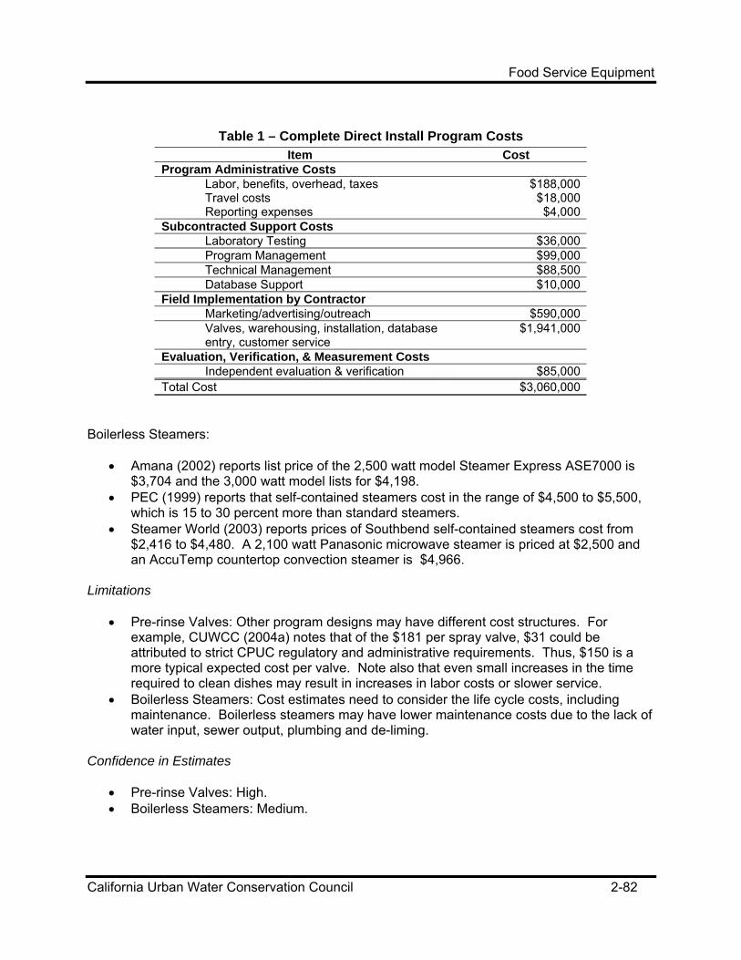
Food Service Equipment
California Urban Water Conservation Council 2-82
Table 1 – Complete Direct Install Program Costs Item Cost
Program Administrative Costs Labor, benefits, overhead, taxes $188,000 Travel costs $18,000 Reporting expenses $4,000
Subcontracted Support Costs Laboratory Testing $36,000 Program Management $99,000 Technical Management $88,500 Database Support $10,000
Field Implementation by Contractor Marketing/advertising/outreach $590,000 Valves, warehousing, installation, database entry, customer service
$1,941,000
Evaluation, Verification, & Measurement Costs Independent evaluation & verification $85,000
Total Cost $3,060,000 Boilerless Steamers:
• Amana (2002) reports list price of the 2,500 watt model Steamer Express ASE7000 is $3,704 and the 3,000 watt model lists for $4,198.
• PEC (1999) reports that self-contained steamers cost in the range of $4,500 to $5,500, which is 15 to 30 percent more than standard steamers.
• Steamer World (2003) reports prices of Southbend self-contained steamers cost from $2,416 to $4,480. A 2,100 watt Panasonic microwave steamer is priced at $2,500 and an AccuTemp countertop convection steamer is $4,966.
Limitations
• Pre-rinse Valves: Other program designs may have different cost structures. For example, CUWCC (2004a) notes that of the $181 per spray valve, $31 could be attributed to strict CPUC regulatory and administrative requirements. Thus, $150 is a more typical expected cost per valve. Note also that even small increases in the time required to clean dishes may result in increases in labor costs or slower service.
• Boilerless Steamers: Cost estimates need to consider the life cycle costs, including maintenance. Boilerless steamers may have lower maintenance costs due to the lack of water input, sewer output, plumbing and de-liming.
Confidence in Estimates
• Pre-rinse Valves: High. • Boilerless Steamers: Medium.

Food Service Equipment
California Urban Water Conservation Council 2-83
2.12.5 Water Savings Calculation Formula(s) Calculations Pre-rinse Valves: Savings is calculated by multiplying hours per day of operation by savings per hour. Savings per hour is estimated as the difference between the flow rates of the water efficient valve and a conventional valve.
Water Savings = Hours_Use * Savings_per_Hour where:
• Water Savings is savings per day from replacing a conventional pre-rinse valve with a water-efficient valve.
• Hours_Use is the average use per day of the pre-rinse station. • Savings_per_Hour is the saving achieved per hour of operation with the efficient valve.
Boilerless Steamers:
Water Savings = High_Water_Use_per_Day – Low_Water_Use_per_Day where:
• High_Water_Use_per_Day is the water consumption of a conventional steamer in the particular restaurant setting under consideration.
• Low_Water_Use_per_Day is the water consumption of the efficient steamer, depending on its technology.
Factors to Consider in Applying the Formula
• Pre-rinse Valves: As with other mechanical/engineering estimates, these figures do not fully reflect behavior that may impact actual savings. For example, if the retention rates are not high, the expected savings will not be achieved. Likewise, behavioral adaptation may also affect savings. For example, the more effective design of pre-rinse nozzles may allow the operator to use shorter rinse times.
• Boilerless Steamers: Consider the full range of performance, including energy and time
savings, food menu, and cook quality. Example Calculation
• Pre-rinse Valves: Using the reduction in the average measured flow rate of 2.24 gpm and an average use per day of 1.27 hours after installation (CUWCC 2004b), savings are 2.8 gallons per day. Note simplifying assumptions: (1) cleaning time is the same before and after installation; (2) pre-installation flow rate is average for small establishments; and (3) the hours of operation are average for small establishments. Field studies indicated both the range of flow rates and the range of hours of operation were large.

Food Service Equipment
California Urban Water Conservation Council 2-84
• Boilerless Steamers: Table 2 shows sample calculations for three different volume food service establishments that replace a conventional steamer with a water efficient model. The example assumes the low volume establishment does not leave the old steamer on all day, thus water consumption is less than the high volume operations. The 3 gallons per day figure for the boilerless steamer is based on closed-system steamer consumption; other results would derive from different types of equipment.
2.12.6 Questions to Ask Pre-rinse Valves:
• Are savings estimates for the particular model pre-rinse valves installed and replaced? • What is the target customer base and implementation approach? Hard-to-reach
customers or large-scale operations? Direct install or financial incentive? Boilerless Steamers:
• Are savings estimates for a particular model steamer? Technology and performance varies significantly (closed system, convection, microwave, heat on demand, vacuum, etc.)
• What food types are being prepared and is the steamer a good match for that food type? • What is the target customer base and implementation approach? Hard-to-reach
customers or large-scale operations? Direct install or financial incentive? 2.12.7 Sources AccuTemp (Undated, Downloaded April 2003), “Steam’n’Hold User Tips,” AccuTemp Products, Inc. URL: http://www.accutemp.net/steamertips. Amana (2001), “Discover the Affordable and Simple Way to Steam, Form No. ACCRR0214,” Amana Commercial Products Division. Amana (2002), “Foodservice Oven Price List – Effective 12/30/02: Form No. ACRR0254,” Amana Commercial Products, Amana, Iowa. CUWCC-FSTC (2002), “CUWCC-FSTC Pre-Rinse Spray Valve Specification VS 1.0,” California Urban Water Conservation Council – Food Service Technology Center, August 28.
Food Service Category
Conventional Steamer Water Use (gals/day)
Water Efficient Steamer Use
(gals/day)
Savings Per Steamer (gal/day)
Small Volume 100 3.0 97.0 Medium Vol. 200 3.0 197.0
High Vol. 300 3.0 297.0
Table 2 - Savings (gpd) by Water-Efficient Steamers

Food Service Equipment
California Urban Water Conservation Council 2-85
CUWCC (2004a), “A Report on Potential Best Management Practices,” prepared for the California Urban Water Conservation Council by Koeller and Company, August. CUWCC (2004b), “Evaluation, Measurement & Verification Report for the CUWCC Pre-Rinse Spray Head Distribution Program,” prepared for the California Urban Water Conservation Council by SBW Consulting, Inc., May. See also letter to CPUC from SBW Consulting, Inc. with minor revisions to program savings results (June, 11, 2004). Dickinson, M.A. and J. Koeller (2003), “Achieving Energy and Water Savings in Food Service Operations: The Pre-Rinse Spray Valve Replacement Program.” DPPEA (Undated, Downloaded April 2003), “Water Management Options: Kitchen and Food Preparation,” Division of Pollution Prevention and Environmental Assistance, North Carolina Department of Environment and Natural Resources. URL: http://www.p2pays.org. EBMUD (2002), “Proposition 13 Grant Proposal for Programs for the Installation of Pre-Rinse Spray Heads and Water and Energy Efficient Dishwashers for the Food Service Industry,” East Bay Municipal Utility District, March. EDID (2002), “Proposition 13 2003 Urban Water Conservation Grant Proposal for Commercial, Industrial, and Institutional Direct Install Zero-Water Consumption Urinal Replacement and Commercial and Industrial Direct Install Low-Flow Pre-Rinse Spray Nozzle Replacement Project,” El Dorado Irrigation District, December. FSTC (Undated, Downloaded April 2003), “Steamers,“ Food Service Technology Center. URL: http://www.pge.com/003_save_energy/pdf/steamers.pdf. PEC (1999), “Self-Contained Countertop Steamer: A Pacific Energy Center Factsheet,” Pacific Energy Center, Pacific Gas and Electric Company. URL: http://www.pge.com/pec. SCVWD (Santa Clara Valley Water District, 2002), “Water Use Efficiency Program Annual Report: Fiscal Year 2001-2002.” Steamer World (Undated, Downloaded April 2003), “Countertop Steamers – Steamer World,” Restaurant Equipment World, Orlando, FL. URL: http://www.steamerworld.com/index-countertopsteamers.html. Waterloo (2005), “Pre-Rinse Spray Valve Pilot Study,” prepared for the Regional Municipality of Waterloo, Ontario, Canada by Veritec Consulting, Inc, January.

Self-Closing Faucets
California Urban Water Conservation Council 2-86
2.13 Self-Closing Faucets 2.13.1 Device/Activity Description Self-closing faucets are based on one of two technologies. The first involves a spring-loaded faucet lever that closes the faucet in a prescribed period of time after it is opened. The second technology involves an infrared (IR) sensor, which turns on the water only as long as it detects hands are under the faucet. Both faucets save water compared to conventional low flow faucets by reducing the average length of time the faucet is opened (“self-closing savings effect”). Since both types are made to meet low flow standards, the faucets save more water when they replace old high flow faucets (“low flow savings effect”). Spring-loaded self-closing faucets are less expensive, although the IR technology is thought to save more water. Self-closing faucets are targeted primarily at CII sites, such as airports, schools, movie theaters, and restaurants. 2.13.2 Applicable BMPs BMP 9 – Conservation Programs for Commercial, Industrial, and Institutional Accounts. In addition to activity-based criteria to determine implementation status, BMP 9 also calls for water-savings performance targets. An agency is considered “on schedule” if their CII accounts show reduction of 10% of baseline within 10 years. BMP 9 estimates the reduction in gallons per employee per day in the Year 2000 to be 12% for commercial and 15 % for industrial water use (from 1980 to 2000). 2.13.3 Available Water Savings Estimates Summary of Individual Studies Behling and Bartilucci 1992 analyze the impact of water-efficient fixtures on office water consumption. The study considers common water using fixtures in an office setting, including toilets, urinals, sinks. Other water consuming activities are factored out in the water savings estimation, including irrigation and cooling water. The study estimates the water use per wash for old (pre-1980 high flow) faucets based on 3 gallons per minute flow for 10 seconds. McCuen 1975, as reported in Waterplan 1988, determines that self-closing faucets reduce water consumption by “up to 50 percent” compared to conventional low flow faucets. Waterplan 1988 uses a “conservative” estimate of 25 percent water savings. NOTES: Since all faucets sold currently are low flow faucets, the incremental active conservation for new faucet installations is the difference between low flow and low flow self-closing faucets--the self-closing savings effect. For replacement of old (high flow) faucets, the incremental active conservation savings is the self-closing savings effect plus any increase in the rate of replacement induced by the active program.

Self-Closing Faucets
California Urban Water Conservation Council 2-87
Persistence No study considering the persistence of savings from self-closing faucets has been found. Possible sources of savings decay might include increased number of malfunctions of self-closing devices over time. Limitations Future efforts should include a search for existing estimates and/or empirical estimation the number of washes per day per fixture and water use per wash for high and low flow fixtures, and for self-closing faucets. Persistence of savings should also be assessed. Confidence in Estimates Low. 2.13.4 Program and Device/Activity Cost Estimates Program Costs Participant program costs may include:
• Cost of purchase and installation of the faucet if not fully subsidized Supplier program costs may include:
• Faucet and purchase of faucets if supplier shares costs • Administration • Contractors • Marketing
The following are professional judgments of costs by conservation program coordinators and managers, as reported in A&N Technical Services (1995):
• Infrared: $200 • Spring valve: $50
Note that these costs are the full cost of the fixture. The incremental cost is difference between the self-closing and the conventional low flow faucet because code requires low flow faucets. Limitations In addition to updating with recent vendor cost estimates, these figures do not reflect differences in maintenance costs, if there are such differences. Confidence in Estimates Low.

Self-Closing Faucets
California Urban Water Conservation Council 2-88
2.13.5 Water Savings Calculation Formula(s) Calculations Savings is calculated by multiplying washes per day by water savings, estimated as the difference between the self-closing faucet and what would have been installed otherwise. For example, for replacement of an old high flow faucet with an IR self-closing faucet, the equation is: SHigh_to_IRLow = Washes_per_Day * (GP_Wash_High_Flow_Faucet -(GP_Wash_IRSelfClosing_Faucet) where:
• SHigh_to_IRLow is savings per day from replacing high with an IR self-closing faucet. • Washes_per_Day is the average washes per day at a faucet during a working day. • Gallons_per_Wash is in units of gpd per self closing faucet
For sample installations, savings are calculated based on the above table plus the number of working days per year and the percent of the self-closing faucets that are replacing otherwise low-flow faucets: SSample = ((Percent_Low * SLow_to_IRLow) + ((1 - Percent_Low) * SHigh_to_IRLow)) * Working_Days_per_Year / 365 where:
• Working_Days_per_Year are the days of operation for a typical faucet. For example, faucets in office buildings are assumed to operate 260 days per year.
• Percent_Low is the percent of self-closing faucets that replace low flow faucets, including new installations and replacements of existing low flow faucets.
Factors to Consider in Applying the Formula As with other mechanical/engineering estimates, these figures do not fully reflect behavior that may impact actual savings. For example, if spring loaded faucets run longer than needed for brief hand washes, actual savings may not be what is anticipated. Example Calculation Table 1 - Savings by Washes per Day is calculated with the following assumptions: Gallons_per_Wash is (in units of gpd per self closing faucet) for old high flow faucets .5gpd (Behling and Bartilucci 1992); for new faucets .33gpd (Behling and Bartilucci 1992), for new faucets with IR self closing .2gpd (Based on McCuen 1975; Waterplan 1988 and judgment), and for new faucets with spring self closing .25gpd (McCuen 1975 and Waterplan 1988). Tables 2 and 3 - Sample Installations are calculated for a range of assumptions using the second formula presented above.
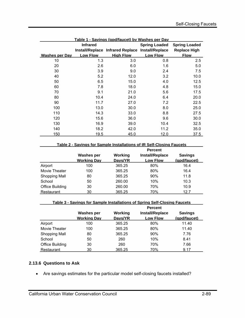
Self-Closing Faucets
California Urban Water Conservation Council 2-89
2.13.6 Questions to Ask
• Are savings estimates for the particular model self-closing faucets installed?
Washes per Day
Infrared Install/Replace
Low FlowInfrared Replace
High Flow
Spring Loaded Install/Replace
Low Flow
Spring Loaded Replace High
Flow10 1.3 3.0 0.8 2.5 20 2.6 6.0 1.6 5.0 30 3.9 9.0 2.4 7.5 40 5.2 12.0 3.2 10.0 50 6.5 15.0 4.0 12.5 60 7.8 18.0 4.8 15.0 70 9.1 21.0 5.6 17.5 80 10.4 24.0 6.4 20.0 90 11.7 27.0 7.2 22.5 100 13.0 30.0 8.0 25.0 110 14.3 33.0 8.8 27.5 120 15.6 36.0 9.6 30.0 130 16.9 39.0 10.4 32.5 140 18.2 42.0 11.2 35.0 150 19.5 45.0 12.0 37.5
Washes per Working Day
Working Days/YR
Percent Install/Replace
Low FlowSavings
(gpd/faucet)Airport 100 365.25 80% 16.4Movie Theater 100 365.25 80% 16.4Shopping Mall 80 365.25 90% 11.8School 50 260.00 10% 10.3Office Building 30 260.00 70% 10.9Restaurant 30 365.25 70% 12.7
Washes per Working Day
Working Days/YR
Percent Install/Replace
Low FlowSavings
(gpd/faucet)Airport 100 365.25 80% 11.40Movie Theater 100 365.25 80% 11.40Shopping Mall 80 365.25 90% 7.76School 50 260 10% 8.41Office Building 30 260 70% 7.66Restaurant 30 365.25 70% 9.17
Table 1 - Savings (gpd/faucet) by Washes per Day
Table 2 - Savings for Sample Installations of IR Self-Closing Faucets
Table 3 - Savings for Sample Installations of Spring Self-Closing Faucets

Self-Closing Faucets
California Urban Water Conservation Council 2-90
2.13.7 Sources A&N Technical Services (1995) Pekelney, D.M., and T.W. Chesnutt, “Reference Document: Program Design Tool and Savings Estimates,” prepared for the Metropolitan Water District of Southern California. Behling, P.J., and N.J. Bartilucci, “Potential Impact of Water-Efficient Plumbing Fixtures on Office Water Consumption,” Journal of the American Water Works Association, October 1992. McCuen, R.H., R. C. Sutherland, and J.R. Kim, “Forecasting Urban Water Use: Software for Water Management Planning,” prepared for California Department of Water Resources, November 1988. Waterplan (1988) Synergic Resources Corporation, “Waterplan Benefit/Cost Analysis Software for Water Management Planning,” prepared for California Department of Water Resources, November.

Ultra Low Flush Toilets (CII)
California Urban Water Conservation Council 2-91
2.14 Ultra Low Flush Toilets (CII) 2.14.1 Device/Activity Description “Ultra-low-flush” (ULF) toilets are low-water-using toilets. Specifically, ULF toilets must use no more than 1.6 gallons per flush. 2.14.2 Applicable BMPs
• BMP 9 – Commercial, Industrial, Institutional. 2.14.3 Available Water Savings Estimates Summary of Individual Studies CUWCC commissioned a study of CII ULF toilet savings that estimated gallons per day savings in a number of different market segments (Hagler Bailly 1997). These results of statistical analysis of 1,320 CII sites in ten agencies in Northern, Central and Southern California are summarized in Table 1.
Veritec Consulting (2002) reports that water consumption was decreased by 65% with the installation of Caroma dual-flush toilets at 459 Bigelow St. in Port Perry, Canada.
Market Segment
Estimated Savings (gpd)
90% Confidence Interval
Wholesale 57 19-94Food Store 48 37-59Restaurant 47 36-58Retail 37 33-42Automotive 36 22-50Multiple Use 29 14-45Religious 28 20-37Manufacturing 23 15-32Health Care 21 13-28Office 20 17-23Miscellaneous 17 11-23Hotel/Motel 16 11-20Source: Hagler Bailly (1997)
Table 1 - Savings per CII ULFT Installed

Ultra Low Flush Toilets (CII)
California Urban Water Conservation Council 2-92
Engineering Technologies Canada (2001) found water savings of 46 to 60 percent compared to the existing 13 liter toilets in public schools. Persistence No study estimating the persistence of conservation savings from CII ULFTs has been found. Limitations This methodology may not work well if the industry categories available differ from those used in the CUWCC CII ULFT Study. To support this statement, the reader should note the wide variability of savings estimates documented within this sector. Confidence in Estimates Good. 2.14.4 Program and Device/Activity Cost Estimates Program Costs Participant program costs may include:
• Cost of ULF toilet and installation not reimbursed by rebate Supplier program costs may include:
• Staff time to administer rebate program • Rebate incentive • Administration • Contractors • Marketing
A&N Technical Services (1995) reports that commercial ULF toilets retail for $150 to $170. The purchase cost estimate comes from the direct installation program in the City of Santa Monica (1989, 1992) and assumes that all installed commercial ULF toilets were flushometer valve-type. Since both flushometer-valve and gravity-fed toilets are used in commercial applications, the $170 purchase cost estimate represents an upper bound. Gravity-fed commercial ULF toilet costs are about the same as multi-family residential toilets. SCVWD (2005) reports they are paying a vendor $270 per CII high efficiency toilet in a direct installation program targeting high volume customers such as restaurants. The fee includes volume measurement to assure the toilet to be replaced is 2.5 gpf or higher, removal and disposal of the old toilet, and installation of a new toilet. The new toilet is a Mansfield 1.0 gpf high efficiency toilet with a Sloan valve.

Ultra Low Flush Toilets (CII)
California Urban Water Conservation Council 2-93
MWDSC (2005) reports that the vendor fee for administering the ULF toilet rebate portion of their CII conservation Pilot Program (ending December 31, 2004) is $24. This fee includes the administration and processing of the rebates, reporting to member agencies, their retailers--and customer service to these agencies, customer service to the end user customer, and the money float for fronting the rebate checks. The fee does not include marketing and overhead costs, which are combined with other elements of the rebate program. Prices for purchasing heavy-duty commercial fixtures range from $325 to more than $600 depending on the type and materials (e.g., American Standard 2005). Limitations Limitations include generalizations about volume purchases and discounts, rates of growth in new facilities and old fixture retrofits (natural replacement), and background saturation (free riders) that are not consistent with those in the study areas. Confidence in the Estimates High, although more research needs to be done on the persistence of savings at different levels of background saturation. 2.14.5 Water Savings Calculation Formula(s) Calculations The general core variables among the market segmented models included in CUWCC sponsored study (Hagler Bailly 1997) are in the following function: Monthly_Water_Use (ccf) = f(Number_of_Retrofits_Installed, Net_Irrigation_Requirements, Region, Season, Time_Trend) Additional variables in one or more market segment models include:
• change in facility operating hours • change in number of visitors at facility • change in total number of employees • change in gender composition of employees • change in production process • extended interruptions in water service • occurrence of major water leaks • change in number of faucet aerators or showerheads in facility • change in efficiency level of urinals • changes to size or type of irrigation system • other changes at facility that could affect water use

Ultra Low Flush Toilets (CII)
California Urban Water Conservation Council 2-94
Factors to Consider in Applying the Formula This formula is meant to be used in the context of statistical estimation of conservation savings. Separate models should be constructed for market segments to account for the great heterogeneity. Example Calculation Refer back to Table 1 for a demonstration of how the equations have been used in a statistical analysis of CII ULFT savings. 2.14.6 Questions to Ask
• Are there other agencies that you can partner with to make your program more cost effective?
• Does your agency have access to grant or other partnership type funding? • What is the age of the building stock in the relevant service area (pre- or post-code)? • Will your program be a free distribution; co-pay (customer and agency share in the cost);
direct install; or rebate? • Will your program be conducted using agency personnel or contracted out? • Will your agency limit the approved models to those toilets that have been tested for long
term water savings and customer satisfaction? • Are installations verified? • Will results be tied to a customer specific database (customer conservation screen)? • Are you going to design and maintain a database covering all participants and program
results? • Is this program in combination with other measures (e.g., CII surveys, pricing)? • Can you influence how the cost of this program is accounted for? If capitalized, the cost
impact will be spread over “x” number of years and reduce the rate impact. If expensed, will the cost of your program have to be recovered in one year?
• When applying an existing savings estimate, how similar is the service area in terms of socioeconomic characteristics and conditions?
2.14.7 Sources A&N Technical Services (1995) Chesnutt, T.W., C.N. McSpadden, and A. Bamezai, Ultra Low Flush Toilet Programs: Evaluation of Program Outcomes and Water Savings, A report for the Metropolitan Water District of Southern California, July. American Standard (2005), Direct sales prices reported at URL: www.americanstandard-us.com. Engineering Technologies Canada, Ltd., “Evaluation of Ultra-Low Flow (6 Litre) Gravity Toilets in Two Schools,” for Prince Edward Island Department of Fisheries, Aquaculture and Environment, November 2001.

Ultra Low Flush Toilets (CII)
California Urban Water Conservation Council 2-95
Hagler Bailly Services (1997), The CII ULFT Savings Study, sponsored by the California Urban Water Conservation Council, August. Horner, R. and T., “The Water-Efficiency Industry”, Plumbing Systems and Design, May/June 2004. Santa Monica (1989), “Recommendation to Approve the Residential Plumbing Fixture Rebate Program,” Proposal to the Mayor and City Council from City Staff, City of Santa Monica, July 25. Santa Monica (1992), “Recommendation to Approve Phase II of the BAYSAVER Plumbing Fixture Rebate Program,” Proposal to the Mayor and City Council from City Staff, City of Santa Monica, February 11. Veritec Consulting, Inc., “Savings Associated with Installation of Dual-Flush Toilets in Apartment Building, 459 Bigelow Street, Port Perry,” letter to Durham Region Works Department, Whitby, Ontario, November 2002. Woods, J.E., and H.W. Hoffman, “Putting Your Money Where Your Mouth Is,” AWWA Water Resources Conference Proceedings, 2004. SCVWD (2005), Telephone conversation with Karen Morvay, Conservation Staff at the Santa Clara Valley Water District, March 14. MWDSC (2005), Telephone conversation with Bill McDonnell, Conservation Staff at the Metropolitan Water District of Southern California, March 14.

Urinals
California Urban Water Conservation Council 2-96
2.15 Urinals 2.15.1 Device/Activity Description Two water saving urinal technologies are (1) low flow valves that utilize less water than conventional valves and (2) non-water-consuming urinals. 2.15.2 Applicable BMPs In addition to activity-based criteria to determine implementation status, BMP 9-Commercial, Industrial, and Institutional Accounts also calls for water-savings performance targets. An agency is considered “on schedule” if their CII accounts show reduction of 10% of baseline within 10 years. BMP 9 estimates the reduction in gallons per employee per day in the Year 2000 to be 12% for commercial and 15 % for industrial water use (from 1980 to 2000). 2.15.3 Available Water Savings Estimates Summary of Individual Studies Behling and Bartilucci (1992) analyze the impact of water-efficient fixtures on office water consumption. The study considers common water using fixtures in an office setting, including toilets, urinals, and sinks. Other water consuming activities are factored out in the water savings estimation, including irrigation and cooling water. The study reports the water use per flush for old (pre-1980 high flow) urinals as 1.5 to 3.0 gallons per flush and new water efficient urinals as 1.0 gallons per flush. The City of Bellevue (1992a and 1992b) analysis considered the replacement of 28 urinal flush valves. The old valves ranged between 1.5 and 2.0 gallons per flush and the new valves used 1 gallon per flush. The setting was a city office building and the analysis was conducted in 1993. The analysis measured building water savings by comparing water use before and after installation of the water saving devices. As reported in PMCL (1994), there is no indication that water use was measured at the individual fixture level or that water savings at the building level was controlled for other explanatory variables such as work force mix and employment. Persistence No study considering the persistence of savings from low flow urinal valves or non-water-consuming urinals has been found. Limitations Future efforts should include a search for existing estimates and/or empirical estimates of the number of flushes per day per fixture, and water use per wash for high and low flow fixtures. Persistence of savings should also be assessed.

Urinals
California Urban Water Conservation Council 2-97
Confidence in Estimates Low. 2.15.4 Program and Device/Activity Cost Estimates Program Costs Participant program costs may include:
• Cost of purchase and installation of the valves and urinals if not fully subsidized Supplier program costs may include:
• Valves and urinals purchase or cost share • Administration • Contractors • Marketing
The following are professional judgments of costs by conservation program coordinators and managers, as reported in A&N Technical Services (1995):
• Low flow valve: $20 (only full flush valve replacement should be considered, cost approx. $60-80 each)
• Non-water-consuming urinal: $100-$400 Limitations The long term maintenance costs and life span of this new class of fixtures has yet to be assessed. Confidence in Estimates Medium-Low. 2.15.5 Water Savings Calculation Formula(s) Calculations Savings is calculated by multiplying flushes per day by water savings, estimated as the difference between the low flow valve (or non-water-consuming urinal) and existing installed value. For example, for replacement of an old high flow urinal with low-flow valve, the equation is: SHigh_to_Low = Flushes_per_Day * (GP_Flush_High_Flow_Urinal - GP_Flush_Low_Flow_Urinal)

Urinals
California Urban Water Conservation Council 2-98
For replacing a low flow valve with a non-water-consuming urinal, the equation is: SLow_to_No = Flushes_per_Day * (GP_Flush_Low_Flow_Urinal - 0) Savings from replacing a high flow valve with a low flow valve are calculated based on Table 1, and the number of working days per year. Since low flow valves are required in California Code, new construction valve installations are not considered active conservation. Since non-water-consuming urinals save more water than low flow valves, savings depend on the percent of non-water-consuming urinals that are replacing otherwise low-flow urinals, rather than high flow urinals: SSample = ((Percent_Low * SLow_to_No) + ((1 - Percent_Low) * SHigh_to_No)) * Working_Days_per_Year / 365.25 where:
• Flushes_per_Day is the average number of flushes per urinal during a working day. • Working_Days_per_Year are the days of operation for a typical urinal. • Percent_Low is the percentage of non-water-consuming urinals that replace low flow
urinals, including new installations that would have been low flow, and replacements of existing low flow urinals.
Factors to Consider in Applying the Formula As with other mechanical/engineering estimates, these figures do not fully reflect behavior that may impact actual savings, such as double flushing. Example Calculation For Table 1 - Savings by Flushes per Day and for Tables 2 and 3 - Sample Installations, the following assumptions are used:
• Flushes_per_Day, Working_Days_per_Year, and Percent_Low urinals are hypothetical values for this numerical example.
• Gallons_per_Flush is for high flow urinal valve 1.5 to 2.0 gallons per flush (Bellevue 1992a and 1932b; Behling and Bartilucci 1992); for low flow urinal valve 1 gallon per flush (Bellevue 1992a and 1932b; Behling and Bartilucci 1992); and for non-water-consuming urinal 0 gallons per flush.
• Working_Days_per_Year are assumed to operate 260 days per year.
• Percent_Low is the percent of non-water-consuming urinals that replace low flow urinals, including new installations that would have been low flow urinals and replacements of existing low flow urinals.

Urinals
California Urban Water Conservation Council 2-99
Flushes per DayLF Valve
Replace High FlowWaterless Urinal
Replace Low FlowWaterless Urinal
Replace High Flow5 3.8 5.0 8.810 7.5 10.0 17.515 11.3 15.0 26.320 15.0 20.0 35.025 18.8 25.0 43.830 22.5 30.0 52.535 26.3 35.0 61.340 30.0 40.0 70.045 33.8 45.0 78.850 37.5 50.0 87.555 41.3 55.0 96.360 45.0 60.0 105.065 48.8 65.0 113.870 52.5 70.0 122.575 56.3 75.0 131.3
Table 1 - Savings by Flushes per Day
Flushes per Working Day Working Days/yr Savings (gpd/urinal)
Airport 50 365.25 37.50Movie Theater 50 365.25 37.50Shopping Mall 40 365.25 30.00School 25 260.00 13.35Office Building 15 260.00 8.01Restaurant 15 365.25 11.25
Table 2 - Savings for Sample Installationsof Low Flow Urinal Valves
Note: Flushes_per_Day, Working_Days_per_Year, and Percent_Low urinals are hypothetical values for this numerical example.
Flushes per Working Day Working Days/yr
Percent Replace Low Flow
Savings (gpd/urinal)
Airport 50 365.3 80% 57.50Movie Theater 50 365.3 80% 57.50Shopping Mall 40 365.3 90% 43.00School 25 260.0 10% 30.53Office Building 15 260.0 70% 16.11Restaurant 15 365.3 70% 18.38
Table 3 - Savings for Sample Installations of Waterless Urinals
Note: Flushes_per_Day, Working_Days_per_Year, and Percent_Low urinals are hypothetical values for this numerical example.

Urinals
California Urban Water Conservation Council 2-100
2.15.6 Questions to Ask • Are there other agencies that you can partner with to make your program more cost
effective? • Does your agency have access to grant or other partnership type funding? • Will your program be a free distribution; co-pay (customer and agency share in the cost);
direct install; or rebate? • Will your program be conducted using agency personnel or contracted out? • Will your agency limit the approved models to those that have been tested for long term
water savings and customer satisfaction? • Are installations verified? • Will results be tied to a customer specific database (customer conservation screen)? • Are you going to design and maintain a database covering all participants and program
results? • Is this program in combination with other measures (e.g., CII surveys, pricing)? • Can you influence how the cost of this program is accounted for? If capitalized, the cost
impact will be spread over “x” number of years and reduce the rate impact. If expensed, will the cost of your program have to be recovered in one year?
• When applying an existing savings estimate, how similar is the service area in terms of socioeconomic characteristics and conditions?
2.15.7 Sources Behling, P.J., and N.J. Bartilucci (1992), “Potential Impact of Water-Efficient Plumbing Fixtures on Office Water Consumption,” Journal of the American Water Works Association, October 1992. Bellevue (1992a) Public Works Department--Utility Services and Property Services Division, “City Building Toilet and Urinal Valve Retrofit Benefit-Cost Analysis,” Bellevue, WA. Bellevue (1992b) Public Works Department--Utility Services and Property Services Division, “City Building Retrofit Project,” Bellevue, WA. PMCL (1994) Planning and Management Consultants, “Urban Water Conservation Programs Volume I: Annotated Bibliography,” September 1994. Sponsored by U.S. Army Corps of Engineers, U.S.G.S., MWD of Southern California, Southern Nevada Water Authority, CUWA, Phoenix Water Services Department, AWWA. A&N Technical Services (1995) Pekelney, D.M., and T.W. Chesnutt, “Reference Document: Program Design Tool and Savings Estimates,” prepared for the Metropolitan Water District of Southern California.

Large Landscape
California Urban Water Conservation Council 2-101
2.16 Large Landscape 2.16.1 Device/Activity Description Large landscape conservation programs target outdoor water use. In practice, “large” often refers to a land parcel greater than 2 or 3 acres with significant landscaping. Sometimes large landscapes are metered separately from non-landscape water consumption; the term “dedicated meter” is often used to refer to meters dedicated to measure landscape end uses11. Large landscape programs can take on many forms and involve site visits, training, device adjustment, upgrading, or water budgets. Devices and activities include centralized computer control, moisture sensors (akin to a water “thermostat” placed in the soil), rain shut-off switches (precipitation causes a switch to interrupt automatic irrigation schedules), telephone connections to California Irrigation Management Information System (CIMIS) information, and numerous other technologies. Some large landscape programs include budget-based rates and/or other economic incentives such as equipment rebates. CIMIS data can be used in several different types of large landscape conservation programs. One program includes a water audit to determine where mechanical improvements and irrigation scheduling can reduce water consumption. The audit may include “catch cone” tests and distribution uniformity tests. CIMIS data may be accessed periodically and utilized in a computer program to determine the appropriate adjustments to irrigation scheduling. Another program involves irrigation management training only, without a comprehensive water audit. A workshop or training session is held where instruction is presented on how to access and use information on an irrigation “hot line,” along with lookup tables, to determine irrigation levels. CUWCC published its “Handbook: A Guide to Implementing Large Landscape Conservation Programs,” to provide additional information regarding BMP 5 and its implementation (CUWCC 1999). 2.16.2 Applicable BMPs BMP 5 – Large Landscape Water Audits and Incentives call for suppliers to implement conservation methods that are at least as effective as a set of actions. These actions include identifying, contacting, and auditing all large landscape sites, providing incentives, follow-up audits, and multilingual training (in summary). To make the case that a large landscape conservation program fulfills BMP 5, one would have to either a) implement the same provisions listed in the BMP, or b) calculate savings and determine whether they are equivalent to the
11 In this document the term “dedicated meters” will refer exclusively to landscape dedicated meters. The term "submetering" will refer to multi-family connections with submeters for each housing unit. If the multi-family has a dedicated meter for landscape, the term dedicated meter will still refer to the landscape meter (not submeter). To summarize, this document will use the following nomenclature:
• submetering: meters on each unit of a multi-family buildings • dedicated meters: dedicated landscape meters • universal metering: addition of water meters for customers that have no meters.

Large Landscape
California Urban Water Conservation Council 2-102
savings from the BMP 5 listed measures. The intervention and device savings described in this section could be useful information to calculate savings for the purpose of determining whether a supplier’s large landscape program fulfills BMP5. Note that there are separate requirements for dedicated accounts and mixed-use accounts. 2.16.3 Available Water Savings Estimates Summary of Individual Studies Water-Budget Based Rate Structures, Outreach, Incentives A&N Technical Services (1997) conducted a study of four large landscape conservation programs in Southern California, each involving a water budget based rate structure. The study included a water use analysis based on empirical data collected in cooperation with participating suppliers. Using historical account level water use records and multiple CIMIS climatic measures, climate-adjusted estimates of water savings were developed. The water use analysis was conducted in three steps, where steps 2 and 3 involved developing increasingly refined regression model specifications: (1) raw water use comparison, (2) comparison correcting for customer characteristics and climate, and (3) structural models of the conservation program interventions. The raw water use analysis required careful data analysis to assure the validity of the water consumption measures. Otay Water District experienced a 20 percent decline in water applied to landscapes, Irvine Ranch experienced a 37 percent decline, and Capistrano Valley experienced a 35 percent decline between the pre- and post-program periods (Table 1). Changes in customer characteristics can make important differences in the estimated savings rates. For example, long-term customers showed a smaller decline in mean water use, about 25 percent; newer customers tended to come on line with lower application rates. Simple models to control for climate reduced the estimated change in raw water use from approximately 25 percent to 22 percent. The estimates from the structural model suggest that the combined intervention of water-budget based rate structures and customer outreach programs in Capistrano Valley had the following effects on the pattern of water demand:
• Average water demand was reduced by 18.6 percent (Table 1); • The seasonal peak demand was also reduced, though to a lesser degree than average
daily demand; • Customer demand became more responsive to information about evapotranspiration;
and
Analytic ApproachPercent Water Use
ReductionSimple Model: All Landscape Customers 35%Simple Water Use Model: Long Term Customers 23%Models Controlling for Climate 22%Structural Intervention Model 19%
Table 1 - Capistrano Valley Water District Savings

Large Landscape
California Urban Water Conservation Council 2-103
• Customer demand became less responsive to rainfall. Central Irrigation Systems An analysis was conducted of the water consumption reduction due to the use of a centralized irrigation system installed in the community of Aliso Viejo in Orange County (Western Policy Research 1996). Controlling for climate and landscape size, water consumption was reduced by 34 percent overall compared to the period before the retrofit. Most of the savings was attributed to the sloped areas, which account for 75 percent of the study area. Sloped areas were shown to have a 45 percent reduction in water use compared to no significant reduction in the turf grass areas. Due to the diversity of plant material on sloped areas, the author concludes that it is difficult to optimize irrigation for sloped areas without a central system. Landscape Audits CCWD (1994a and 1994b) measured savings from a landscape audit program that involved visits to irrigated sites by irrigation management experts who made recommendations for conservation change. Among other important findings, the study concluded:
• The degree of excess irrigation is large in the fall season; • Contract landscapers are less efficient in terms of water consumption and irrigation
practices; • Smaller sites (e.g., less than 2 acres) have the potential for a greater percentage water
savings because they are not as well managed as large sites. • Savings from water audits decline rapidly over time.
Water savings were estimated to be 20.6 percent in the first year, 7.7 percent in the second year, and 6.5 percent in the third year. Combined Landscape Management Practices Western Policy Research (1997) reports the results of a statistical analysis of the water saving effects of combinations of landscape management practices. The three categories of landscape management practices include evapotranspiration-based irrigation scheduling, improved system maintenance, and advanced turf grass horticultural practices. The study included 16 sites in similar climate conditions with cool-season turf. Outcomes of the study were measured in terms of conservation savings, turf quality, and root depth. Overall, water consumption was cut in half by the programs, even after controlling for climate. Tiered rates and outreach programs were implemented just prior to the study of conservation practices. For example, the study attributed 30 inches of water savings per year to the inclining block rates and outreach programs. An additional 21.9 inches is attributed to the advanced practices. It is important to note that appearance of turf grass was also evaluated over time by a team of judges, who concluded that appearance actually improved over time. DeSena (1998, as reported in Vickers 2001) reports the outdoor water use of Irvine Ranch Water District customers was reduced by 50 percent as a result of its increasing rate block structure.

Large Landscape
California Urban Water Conservation Council 2-104
A&N Technical Services (2004) reports on the Municipal Water District of Orange County’s Landscape Performance Certification Program (LPCP) for dedicated irrigation meter customers. The program consists of outreach, training, and developing water budgets. The results show customers participating in Phases 1 and 2 of the program saved 367 gallons per day on average (251 gpd – 512 gpd is the 95 percent confidence level). Customers participating in Phases 3 and 4 of the LPCP (after November 2001) saved 765 gallons per day on average (540 gpd – 991 gpd bound the 95 percent confidence interval). The program also showed additional water savings in the peak summer months (up to 1300 gallons per day on the maximum day demand). CIMIS Hot Lines Two programs were conducted by the Marin County Water District, as described in Bourg (1993) and Nelson (1989). The “Irrigation Management Program” contacted the largest irrigation customers, of which 63 agreed to participate in water conservation workshops. Look-up tables were developed by conducting a study to calibrate the reference evapotranspiration to the local vegetation. The workshops were attended by turf managers, who were instructed on how to use the Hot Line and look-up tables to determine the appropriate irrigation level. A water auditor monitored irrigation. The other program involved an on-site audit of commercial/government customers with greater than 100HCF/YR water use to determine opportunities for water conservation. This program involved an initial audit to determine low-cost savings opportunities, then a comprehensive audit with water distribution uniformity and catch cone tests. Turf managers were then trained in how to access CIMIS data periodically and utilized in a computer program to determine the appropriate adjustments to irrigation scheduling. The following summarizes some of the available savings estimates from Bourg (1993) and Nelson (1989): CIMIS Hot Line with Water Audits for Parks and Playing Fields (Customers >400 HCF/YR):
• 16% reduction in expected water usage (government parks) • 7.7% reduction in expected water usage (private park)
CIMIS and Irrigation Management Training for Large Irrigation Customers:
• 10.9% reduction in peak month demand (with Hot Line and training) • 3.6% reduction in peak month demand (with Hot Line, but no training)
Although these water use per acre values are specific to an agency, the savings studies were conducted in Marin County, which has significantly different climate and landscape characteristics than many parts of California; the differences in climate, vegetation, and ETo, limit the generalizability of these results. Turf Replacement Padilla and Torres (2004) report 398 gallons per day participant-weighted average savings at commercial and residential sites from a turf rebate program.

Large Landscape
California Urban Water Conservation Council 2-105
Sovocool and Rosales (2004) report 33% reduction average, and 39% reduction in the summer months in terms of “main meter” overall consumption at single family residences. More relevant for large landscape is the decrease in mean irrigation use only. Irrigation use, in gallons per square foot per year, was 79 at turf sites and 17 at xeriscape sites. The City of Austin (1999) reports average water savings per participant site of 214 gallons per day in the summer compared to preexisting landscapes as a result of their landscape rebate program. Irrigation Controllers MWDSC (2004) performed bench test evaluations of three popular weather-based irrigation controllers. The study concludes that the controllers have the potential to realize significant water savings, but that they still need some adjustment at times. U.C. Extension, Riverside (2004) tested a recent group of weather-based irrigation controllers and their ability to track ETo based irrigation throughout the year: “The results of this study show each controller evaluated adjusted its irrigation schedules through the year roughly in concert with weather and ETo changes, but the magnitudes of their adjustments were not consistently in proportion to the changes in real-time ETo. Unfortunately, no product was able to produce highly accurate irrigation schedules consistently for every landscape setting when compared to research-based reference comparison treatments.” Persistence More research needs to be conducted to develop generalizable estimates of persistence. One study indicates that savings from large landscape audit programs drop off quickly (CCWD 1994). Savings in the same year were 20.6 percent, savings in one season later were only 7.7 percent, and savings two seasons later were 6.5 percent. Limitations One important limitation is the difficulty of distinguishing the savings achieved from the water-budget-based rate structures from the outreach and incentives programs. Since these programs have been implemented concurrently, a more detailed statistical analysis would be needed to determine how much each of the program components contributes to water savings. Confidence in Estimates Medium-Low. The difficulty of generalizing landscape savings is apparent when considering the great diversity in climate among the regions throughout the state. 2.16.4 Program and Device/Activity Cost Estimates Program Costs Participant program costs may include:

Large Landscape
California Urban Water Conservation Council 2-106
• Cost of purchase and installation of landscape efficiency equipment, including
controllers, moisture sensors, one-way valves, sprinkler heads, etc., to the extent they are not financially supported by the water supplier.
Supplier program costs may include:
• Landscape measurement • Financial incentives • Administration • Contractors • Marketing
CUWCC (1999) includes example cost estimates for a water budget program (Table 2) and a water survey program (Table 3). Cost estimates for the water budget program range between $50 and $300 per site, according to the report. Water survey costs range between $500 and
$1500 per site.
TaskFixed Costs
Cost per Site Notes
Inventory of dedicated irrigation meters 1,800$ 30 hours x $60/hour = $1,800Landscape measurement 100$ Assumes field measurement method usedBudget calculation 1,200$ 20 hours x $60/hourBudget distribution 12$ $1 per site per monthly billing periodMonitoring and tracking 30$ 0.5 hours x $60/hourTotal 3,000$ 142$ Reproduced from CUWCC 1999.
Table 2 - Example Costs of Water Budget Program
TaskFixed Costs
Cost per Site Notes
Inventory of CII Mixed Use Accounts 2,400$ 40 hours x $60/hourTargeting 2,400$ 40 hours x $60/hourMarketing 2,400$ 25$ 40 hours x $60/hour plus direct costsSurvey Implementation 720$ 12 hours x $60/hourFollow-Up Activities Not Included
Monitoring and Tracking 6,000$ 10$ 100 hours x $60/hour which includes 1
basic analysis Total 13,200$ 755$ Reproduced from CUWCC 1999.
Table 3 - Example Costs of Water Survey Program

Large Landscape
California Urban Water Conservation Council 2-107
A&N Technical Services (1997) also reports the results of a survey of large landscape customers subject to water-budget based rate structures. A mail survey was sent to all separately metered irrigation customers in four Southern California service areas. The inference that can be drawn from the subset of returned surveys to the population is limited by the potential for response bias; inference to other agencies is limited further by the degree to which site characteristics and other conditions are similar to the study. Table 4 shows the results of the customer self-reported estimates of costs of conservation actions: Supplier costs might include computer programming to set up a new rate structure, program design and setup, area measurement, operation, education and outreach, and equipment rebates.
CCWD (1994) reports that auditing a site of up to one-acre costs $310, and $84 for each additional acre at the same site. A detailed breakdown of audit costs in Appendix B of the study is reproduced in Table 5.
Padilla and Torres (2004) report a rebate cost of $.50 per square foot of turf removed, or equivalently $598/AF.
Action Initial Ongoing Initial OngoingAdjusted Timers 482$ 247$ 137$ 77$ Upgrade Equipment 2,571$ 1,540$ 953$ 54$ Repaired Irrigation System 793$ 2,571$ 560$ 399$ External Audit 45$ 126$ 43$ 46$ Other 185$ 77$ 141$ 80$
Table 4 - Mean Reported Costs of ConservationPer AcrePer Customer
Action Hours CostsLabor $28/hr.
Audit 6 Report/Schedule 3
Subtotal 9 252.00$ Administrative Costs 36.00$ Labor Subtotal 288.00$
EquipmentComputer $3200/500 audits 6.40$ Catch Cans, Soil Probe, Pressure Guage, Flags, Wheel, Walkie-Talkie $750/250 audits 3.00$ Milage 30 mi.@ $.28/mi. 8.40$ Mailings 4.00$ Equipment Subtotal 21.80$
Total 309.80$
Table 5 - Cost of Audit for Site with 1 Acre of Turfgrass

Large Landscape
California Urban Water Conservation Council 2-108
Sovocool and Rosales (2004) report that xeriscape maintenance spending (not including water savings) is approximately 1/3 less than turf maintenance spending. De La Piedra (2004) reports on the accuracy and cost of landscape area measurements using multi-spectral imaging. Applied Ecological Services (as reported in Vickers 2001) estimates that a landscape with prairie grasses or native vegetation costs considerably less to maintain than conventional turf grasses--$3,000 per acre over 20 years compared to $20,000 per acre. Limitations Program costs will vary considerably depending on the design of the program. Confidence in Estimates Medium. 2.16.5 Water Savings Calculation Formula(s) Calculations Water_Savings = Savings_Per_Acre * Acres_Per_Site * Number_of_Sites Factors to Consider in Applying the Formula Statistical models, such as those used in A&N Technical Services (1997) are more complex then the simple equation above; however they require extensive data and modeling efforts.
If the objective is to calculate pre-budget water use from data on post-budget water use:
Pre-Budget Use = Post-Budget Use / ( 1 - Average Savings per Landscape Budget %/100)
Example Calculations We provide three sample calculations. The first is based on an empirical study of water budget based landscape conservation programs. This study demonstrates a data- and model-driven method for calculating conservation savings from programs that combine water budget based rate structures with auxiliary program types (rebates, education, etc.). The latter two examples are speculative efforts at quantifying conservation savings of a single program element, such as moisture sensor program. We then summarize evidence for CIMIS hotline programs. Example 1: Empirical Estimation with a Statistical Model Table 1 shows the savings result of the structural model from Capistrano Valley Water District. This model estimates the conservation effect of an “intervention,” composed of a water budget

Large Landscape
California Urban Water Conservation Council 2-109
based rate structure combined with outreach. Since, in this case, both the rate structure and the outreach programs occur together, the statistical analysis cannot identify separate effects of each element of the intervention. Example 2: Rough Estimation of a Savings Parameter, Separately Metered Sites This example, as well as example 3, shows how savings figures can be used in “back of the envelope” calculations to develop rough savings estimates. The examples illustrate how savings estimates can be developed for different definitions of a conservation activity. In this example the activity is a “site” audit, and in example 3 the activity is an “acre” audit. As explained below, the activity is defined differently in these two examples because of the available data: in this example separate meter data are available and in example 3 they are not. A large landscape program is targeted toward 250 separately metered irrigation accounts. Consumption histories from the billing system provide an estimate of average consumption among these sites--approximately 120 hundred cubic feet per monthly billing period. If the savings parameter needs to be expressed in gallons per day, average use per day in HCF/Month is converted to GPD. If the program saves 15 percent of this use, the expected savings per site will be (2,967 X .15 =) 445 GPD.
DAYGl.445 =
DAYGl.2967 x .15
:Siteper Savings CalculateDAYGl.2,967
30.25DAYS748Gl.120 =
MONTHHCF120
30.25DAYS=1MONTH748Gl.=1HCF
:Siteper UseCalculate
≈•⇒
Example 3: Rough Estimation of a Savings Parameter, Separately Metered Sites A large landscape program is targeted toward 250 multi-family complexes whose outdoor water use is not separately metered. Hence, consumption summaries from the billing system represent both indoor and outdoor water use. The complexes each have about 2 acres of irrigated landscape area. On-site audits have shown irrigation of 60 or more inches of water per acre in areas where ETo is only 48 inches per year. This savings potential is 12 inches per acre. Taking a conservative 6 inches per acre savings in practice, we calculate the savings per acre in gallons per day for the audit program:

Large Landscape
California Urban Water Conservation Council 2-110
DAYGl.446
365DAYS325,851Gl. .5 =
YEARFEET.5
365DAYS = 1YEARGl. 325,851 = AF 1
:Acreper SavingsCalculate
≈•⇒
2.16.6 Questions to Ask
• Are there other agencies that you can partner with to make your program more cost effective?
• Are landscape areas on dedicated irrigation meters identified? • Are there CII accounts with mixed-use meters and like accounts without meters
identified? • What are the climatic conditions, and do you have the ETo for determining the right
application of water? • Does your agency have a separate irrigation rate/tariff? • Does your agency already have an established billing system that will accommodate the
use of water budgets? • Will your agency conduct these audits with its own personnel or with an outside
contractor? • What type of water is used: potable or reclaimed? • Is follow-up training and tracking part of the program?
2.16.7 Sources Applied Ecological Services, Inc. Brodhead, Wisconsin (as reported in Vickers 2001). A&N Technical Services (1997), “Landscape Water Conservation Programs: Evaluation of Water Budget Based Rate Structures,” prepared for the Metropolitan Water District of Southern California, September. A&N Technical Services (2004), “Landscape Performance Certification Program: Process and Impact Evaluation,” prepared for the Municipal Water District of Orange County and Metropolitan Water District of Southern California, January. Bourg, J.D., and J.O. Nelson (1993), “Results of Irrigation Audits/Scheduling of the Parks and Playing Fields of Novato California,” Proceedings of CONSERV93: The New Water Agenda, Denver: American Water Works Association, pp. 1019-1024. As reported in PMCL (1994). CCWD (1994a), Contra Costa Water District, “Landscape Water Audit Evaluation,” August 1994. CCWD (1994b), Contra Costa Water District, “Weather Normalized Evaluation,” August 1994. City of Austin, Texas, “Xeriscaping: Sowing the Seeds for Reducing Water Consumption,” prepared for the U.S. Bureau of Reclamation, Austin, Texas May 1999.

Large Landscape
California Urban Water Conservation Council 2-111
CUWCC (1999), “Handbook: A Guide to Implementing Large Landscape Conservation Programs.” De La Piedra, J., “Landscape and Agricultural Area Measurement and Water Use Budgets” AWWA Water Resources Conference Proceedings, 2004. DeSena, M., “ Irvine Ranch Water District Uses Rate Structures to Spur Conservation,” U.S. Water News, vol. 15, no. 21, September 1998. Metropolitan Water District of Southern California, “Weather Based Controller Bench Test Report,” 2004. Nelson, J.O. (1989), “Irrigation Management Program,” North Marin Water District, Novato, CA. As reported in PMCL (1994). Padilla, A., and D. Torres, “Water Savings from a Turf Rebate Program in the Chihuahuan Desert,” AWWA Water Resources Conference Proceedings, 2004. PMCL (1994), “Urban Water Conservation Programs Volume I: Annotated Bibliography,” Planning and Management Consultants, Inc., September. Sovocool, K. and J. Rosales, “A Five-Year Investigation into the Water and Monetary Savings of Residential Xeriscape in the Mojave Desert,” AWWA Water Resources Conference Proceedings, 2004. University of California Cooperative Extension, Riverside, “Evaluation Of Weather-Sensing Landscape Irrigation Controllers” for the Office of Water Use Efficiency, California Department of Water Resources, June 2004. Vickers, A., “Handbook of Water Use and Conservation,” WaterPlow Press, Amherst, 2001. Western Policy Research (1996), “Do Centrally Controlled Irrigation Systems Use Less Water? The Aliso Viejo Experience,” prepared for the Metropolitan Water District of Southern California. Western Policy Research (1997), “Efficient Turf grass Management: Findings from the Irvine Spectrum Water Conservation Study: Statistical Analysis,” prepared for the Metropolitan Water District of Southern California.

System Audits and Leak Detection
California Urban Water Conservation Council 2-112
2.17 System Audits and Leak Detection 2.17.1 Device/Activity Description This conservation activity consists of three possible components:
• System audits • Leak detection • Leak repair
System audits include quantifying all produced and sold water, and may include testing meters, verifying records and maps, and field checking distribution controls and operating procedures (AWWA 1999). The objective is to determine the amount of water that is lost and unaccounted for in the system. System audits may identify losses from:
• Accounting procedure errors • Illegal connections and theft • Malfunction distribution-system controls • Reservoir seepage, leakage, and overflow • Evaporation • Detected and undetected leaks
Leak detection is the process of searching for and finding leaks in the system with sonic, visual, or other indicators. Reviewers have noted that sonic and acoustic leak detection equipment is more accurate for smaller systems than for larger systems. Audits and detection programs incur costs whether or not repairs are made; thus, audits and detection alone do not save water. Conversely, leaks are sometimes discovered without organized audit and detection programs. Finally, reviewers have noted that ”leak prevention” would also be part of these programs, including corrosion control, quality control on materials and installations, and backflow device testing. Kunkel and Beecher (2001) and Flowers (2001) review the challenges of defining water loss in a way that makes reporting meaningful. Farley and Trow (2003, source book) and Trow and Farely (2003, summary paper) provide a comprehensive overview of the IWA approach to leakage management in water distribution systems. 2.17.2 Applicable BMPs BMP 3 – System Water Audits, Leak Detection and Repair calls for prescreening audits, full-scale audits when indicated, and repairs. 2.17.3 Available Water Savings Estimates

System Audits and Leak Detection
California Urban Water Conservation Council 2-113
Summary of Individual Studies The incremental savings of system audits and leak detection are the additional savings from repairs that: a) would not have taken place without the program or b) would have taken place at a later time and perhaps more severely. Moyer (1985) makes the rough assumption that leaks are detected one year earlier than they would have been without the program. Thorton (2002) contains case studies, which report savings and costs for a number of programs conducted in the field. For example, the Moyer et al. (1983) study below is summarized in the Thorton text. Moyer et al. (1983) report the results of six years of leak detection and repair activities at the Westchester Joint Water Works in Mamaroneck, New York as follows: 498 leaks detected, or 10,469 ML water saved, and $239,062 total leak detection and repair costs. Young (as published in Thorton, 2002), found savings of 1,110 cubic meters using advanced water pressure management in a Johannesburg, South Africa. Maddaus, Arsdel, and Woody (2004) report the total system water loss in the Asheville, North Carolina service area was 36 percent for year 2002. Among other results reported, 61 large meters were tested and it was found that 10 meters were un-testable, 16 meters failed, and 35 meters passed. Preliminary results show a 46 percent fail rate for small meters between 5/8” and 1”. Lalonde (2004) reports savings of 6.5 percent on average resulting from pressure management strategies that reduce pressure, on average, 14psi. Thorton (2004) reports savings from one case study (York Region, Toronto, Canada) of 1.57 million gallons per day, equating to a 22 percent savings of the original non-revenue water. A second case study regarding Irvine Ranch Water District single-family residential pressure reduction found 1.9 percent savings and 4.1 percent for those with large landscapes. A third in Sao Paolo, Brazil project annual savings of 671 million cubic meters resulting from installation of pressure stations, increased leak detection and response time, small revenue meter change-outs, large meter change-outs, meter resetting, recovered physical loss, and recovered non physical loss. Bardsley and Lloyd (2004) report 68 million gallons per day savings resulting from installing distribution management areas, pressure reduction, replacing and repairing water mains, leak detection and repair. Rajala (2001) reports on program in Kansas that includes leak detection, meter testing and replacement, and bookkeeping reviews. 50 water audits were conducted and 207 million gallons on annual basis were saved as a result. The cost of the program was $339,136. Persistence No study considering the persistence of savings from leak detection has been found.

System Audits and Leak Detection
California Urban Water Conservation Council 2-114
Limitations The assumptions regarding how much earlier leaks are detected with a program than without a program are not well supported. Confidence in Estimates Low. To obtain reliable estimates of water conservation from leak repair, one needs to measure leakage rates and how they may change over time. 2.17.4 Program and Device/Activity Cost Estimates Program Costs Supplier program costs may include:
• System audits. • Leak detection equipment and labor. • Contractors
AWWA (1999) conclude that the cost of water audits vary widely depending on factors such as the completeness of the audit, the size of the service area, and quality of utility records. In addition to meter testing, the major component of cost is labor by utility staff or consultants. For 12” to 15” meters, reviews reported audit cost from $500-$2,500. A 1994 calibration of a 30” meter cost $600. California water system costs tend to run higher than the national averages reported by AWWA, according to the reviewers. Reviewers also noted that leak prevention activities cost about $150 per test. Materials cost in the range of $500 to $2,000—for example—for installation of back flow devices. As stated before Moyer et al. (1983) results of six years of leak detection, with 498 leaks detected and repaired, cost $239,062. Limitations Leak detection equipment is evolving rapidly and cost data needs to be updated periodically. Confidence in Estimates Medium-Low. 2.17.5 Water Savings Calculation Formula(s)
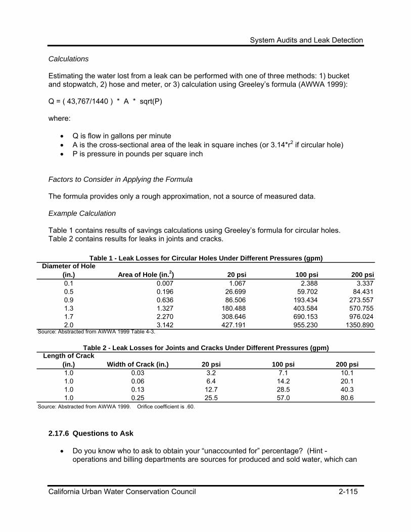
System Audits and Leak Detection
California Urban Water Conservation Council 2-115
Calculations Estimating the water lost from a leak can be performed with one of three methods: 1) bucket and stopwatch, 2) hose and meter, or 3) calculation using Greeley’s formula (AWWA 1999): Q = ( 43,767/1440 ) * A * sqrt(P) where:
• Q is flow in gallons per minute • A is the cross-sectional area of the leak in square inches (or 3.14*r2 if circular hole) • P is pressure in pounds per square inch
Factors to Consider in Applying the Formula The formula provides only a rough approximation, not a source of measured data. Example Calculation Table 1 contains results of savings calculations using Greeley’s formula for circular holes. Table 2 contains results for leaks in joints and cracks.
2.17.6 Questions to Ask
• Do you know who to ask to obtain your “unaccounted for” percentage? (Hint - operations and billing departments are sources for produced and sold water, which can
Diameter of Hole (in.) Area of Hole (in.2) 20 psi 100 psi 200 psi0.1 0.007 1.067 2.388 3.3370.5 0.196 26.699 59.702 84.4310.9 0.636 86.506 193.434 273.5571.3 1.327 180.488 403.584 570.7551.7 2.270 308.646 690.153 976.0242.0 3.142 427.191 955.230 1350.890
Source: Abstracted from AWWA 1999 Table 4-3.
Length of Crack (in.) Width of Crack (in.) 20 psi 100 psi 200 psi1.0 0.03 3.2 7.1 10.11.0 0.06 6.4 14.2 20.11.0 0.13 12.7 28.5 40.31.0 0.25 25.5 57.0 80.6
Source: Abstracted from AWWA 1999. Orifice coefficient is .60.
Table 1 - Leak Losses for Circular Holes Under Different Pressures (gpm)
Table 2 - Leak Losses for Joints and Cracks Under Different Pressures (gpm)

System Audits and Leak Detection
California Urban Water Conservation Council 2-116
be used to calculate a cursory estimate of unaccounted for water. However, a thorough audit process is needed for a fully substantiated estimate of unaccounted for water.)
2.17.7 Sources AWWA (1999), American Water Works Association, “Water Audits and Leak Detection: Manual of Water Supply Practices M 36.” Bardsley, A. and R. Lloyd, “Leakage Reduction: A Proven Alternative Resource. A Yorkshire Water Services UK Three Year Study,” AWWA Water Resources Conference Proceedings, 2004. California Department of Water Resources (1986), “Water Audit and Leak Detection Guidebook,” with the American Water Works Association California – Nevada Section. California Department of Water Resources, “Leak Detection Technology,” Water Conservation News, Spring 2002, URL: http://www.owue.water.ca.gov. Farley, M., and S. Trow, “Losses in Water Distribution Networks – A Practitioner’s Guide to Assessment, Monitoring, and Control,” IWA, April 2003. Flowers, J., “U.S. Environmental Protection Agency’s Interest in the Water System Leakage Issue,” AWWA Conference Proceedings, 2001. Greeley, D.S. (1981), “Leak Detection Productivity,” Reference Number 1981, Water/Emergency & Management, Des Plaines, p. 111 (as noted in AWWA 1990). Lalonde, A. “Use of Flow Modulated Pressure Management in York Region, Ontario to Reduce Distribution System Leakage,” AWWA Water Resources Conference Proceedings, 2004. Lambert, A., “Issues and Needs in Water Loss Reduction,” AWWA Conference Proceedings, 2001. Maddaus, L., J. Van Arsdel, and C. Woody, “Tracking Down Those Water Losses! A Case Study in Asheville North Carolina,” AWWA Water Resources Conference Proceedings, 2004. Moyer, E. et al., “The Economics of Leak Detection and Repair,” originally published in Journal AWWA (vol. 75, no. 1, January 1983) as reported in Thorton (2002, p 241). Moyer, E.E. (1985), “The Economics of Leak Detection: A Case Study Approach,” American Water Works Association. T.K. Rajala, “Kansas Water Plan Programs to Reduce Unaccounted For Water,” AWWA Conference Proceedings, 2001. Thorton, J., “Efficient Water Pressure Management as an Effective Tool for Utilities,” AWWA Water Resources Conference Proceedings, 2004. Thorton, J., “Water Loss Control Manual,” McGraw-Hill, 2002.

System Audits and Leak Detection
California Urban Water Conservation Council 2-117
Trow, S., and M. Farley, “Developing a Strategy for Leakage Management in Water Distribution Systems,” Proceedings of the IWA Conference on Efficiency Use and Management of Urban Water Supply, April 2003. Young, A. “Advanced Water Pressure Management in the Berea-Alexander Park Supply District, Johannesburg, South Africa,” published in Thorton (2002, p 279).

Program Cost Accounting
California Urban Water Conservation Council 3-1
3 Program Cost Accounting This chapter provides guidelines for conservation program cost accounting—including a standard cost template—to encourage complete enumeration and uniform classification of all relevant program costs.12 It also addresses how packaging of devices and activities into a comprehensive conservation program can affect both program costs and program savings. An expanded example is developed to illustrate how program design can impact costs. This example also discusses cost estimation issues such as perspective of analysis, free riders, and cost sharing. Roadmap: The primary emphasis of this chapter is on cost accounting. Material that deals with the more general issues of benefit-cost and cost-effectiveness analyses can be found in the CUWCC Cost-Effectiveness Guidelines document. More detailed examples of cost-effectiveness analysis are also included in Appendix A of this document and in the Cost-Effectiveness Guidelines. Program design can influence program costs, thus, consideration of program design is important to cost estimation. This chapter provides tools to estimate how different program design parameters may affect program costs, as well as providing more general guidance on how to estimate and account for program costs.13 3.1 Templates to Structure Cost Accounting This section provides a two-part template to structure cost measurement and valuation data. The template provides an expanded structure that is consistent with the CEA Guidelines. In section 3.3 is a numerical example of how to utilize the template. Table 3.1 is the first page of the cost template. The rows in this table are grouped into four functional categories: A) Administration, B) Marketing, Advertising, and Outreach, C) Direct Implementation, and D) Evaluation, Measurement, and Verification. The columns are divided into two categories: Utilities (work done in-house) and Contractors (work contracted out). An advantage of this structure is that it forces explicit comparisons between delivery of services by a utility and by contractors. Although such comparisons may be done in the aggregate, rarely are they done side by side.
12 This chapter is based on the following sources, all of which are good references for further information about water conservation program costs: 1) U.S. EPA Water Conservation Plan Guidelines, EPA-832-D-98-001, 1998; 2) CUWCC CEA Guidelines, 1996; 3) Pekelney, Chesnutt, and Mitchell, Cost-Effective Cost-Effectiveness: Quantifying Conservation on the Cheap, June 1996 proceedings of the American Water Works Association; and the AWWA Guidebook for Small and Medium Sized Utilities. 13 Good references that include program design and implementation include the CUWCC BMP Handbook series (Large Landscape, etc.) and Handbook of Water Use and Conservation, Amy Vickers, 2001.

Program Cost Accounting
California Urban Water Conservation Council 3-2
The reader should note that rows and columns may always be added or deleted. For example, one might want several categories of direct implementation materials if the program is multi-faceted, like an indoor and outdoor residential survey. As represented below in Table 3.5, rows may be added if there is cost sharing by another utility and one wishes to make such accounting explicit -- e.g. this could allow an analysis of costs with and without cost sharing. To use the template, organize the program costs into basic accounting units, such as direct labor, materials, administration, and contracted services. The sequence of columns includes the number units (e.g., hours of labor time), the unit cost (e.g., $40 per hour) and their product in the subtotal column. In addition, the column labeled Time is used to indicate at what time the cost is incurred. For example, labor costs for program design may be incurred only in the first year, while labor for implementation may be incurred through all the years of the program. Be sure to always use either calendar year or fiscal year designations. Table 3.2 is the second part of the template where costs can be summed and further accumulated and displayed over time. The first column tracks the elapsed years. Thus, the first year of program implementation would be Year 1 with the costs assumed to be incurred at one time at the end of the year. Program design and planning would take place in Year 0 and earlier. The second column contains the calendar year equivalent (or FY if that is the convention used). A consistent convention such as end of year accounting is highly recommended.
Unit Unit Cost Subtotal Time Unit Unit Cost Subtotal TimeA Administration1 Direct Labor 2 Benefits & Overhead 3 General and Administrative Costs4 Travel 5 Other (specify)
B Marketing, Advertising, and Outreach1 Direct Labor2 Benefits & Overhead3 Brochures and Marketing Material4 Training materials (for canvassers/installers)5 Letters, Postage, Mailing Costs6 Other (specify)
C Direct Implementation1 Direct Labor 2 Benefits & Overhead3 Materials4 Rebates or other payments5 Travel6 Other (specify)
D Evaluation, Measurement, and Verification1 Measurement: tracking of water use2 Verification: field inspections3 Evaluation: savings analysis4 Other (specify)
Notes:
Table 3.1 - CUWCC Program Cost Accounting Template (Categories)
1. This template provides a recommended form for cost accounting. It may be adapted as needed.2. Cost accounting should distinguish between one time costs and recurring costs. Where needed, a separate version for each can be developed as inputs for a final annualized version.
Item LineUtilities Contractors
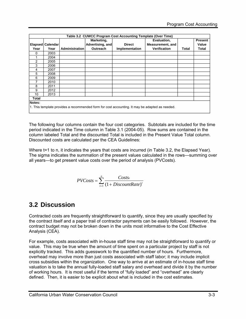
Program Cost Accounting
California Urban Water Conservation Council 3-3
The following four columns contain the four cost categories. Subtotals are included for the time period indicated in the Time column in Table 3.1 (2004-05). Row sums are contained in the column labeled Total and the discounted Total is included in the Present Value Total column. Discounted costs are calculated per the CEA Guidelines: Where t=1 to n, it indicates the years that costs are incurred (in Table 3.2, the Elapsed Year). The sigma indicates the summation of the present values calculated in the rows—summing over all years—to get present value costs over the period of analysis (PVCosts).
3.2 Discussion Contracted costs are frequently straightforward to quantify, since they are usually specified by the contract itself and a paper trail of contractor payments can be easily followed. However, the contract budget may not be broken down in the units most informative to the Cost Effective Analysis (CEA). For example, costs associated with in-house staff time may not be straightforward to quantify or value. This may be true when the amount of time spent on a particular project by staff is not explicitly tracked. This adds guesswork to the quantified number of hours. Furthermore, overhead may involve more than just costs associated with staff labor; it may include implicit cross subsidies within the organization. One way to arrive at an estimate of in-house staff time valuation is to take the annual fully-loaded staff salary and overhead and divide it by the number of working hours. It is most useful if the terms of “fully loaded” and “overhead” are clearly defined. Then, it is easier to be explicit about what is included in the cost estimates.
∑= +
=n
tt
t
teDiscountRaCostsPVCosts
1 )1(
Elapsed Year
Calendar Year Administration
Marketing, Advertising, and
OutreachDirect
Implementation
Evaluation, Measurement, and
Verification Total
Present Value Total
0 20031 20042 20053 20064 20075 20086 20097 20108 20119 2012
10 2013Total
Table 3.2 CUWCC Program Cost Accounting Template (Over Time)
Notes:1. This template provides a recommended form for cost accounting. It may be adapted as needed.

Program Cost Accounting
California Urban Water Conservation Council 3-4
3.3 Numerical Example This example, Table 3.3, is provided to demonstrate in simple numerical terms how to apply the template and the cost accounting and estimation methods developed pursuant to the Memorandum of Understanding (MOU). Table 3.3 is a simple example to communicate the fundamental principles to those new to the subject. More complex examples can be found in
Appendix A and the CEA Guidelines. This example is based on a hypothetical ULF toilet rebate program. It shows the cost template filled in with cost data for a simple program. The second column contains the labels for each cost item. In the Administration cost category, direct labor is presented in units of labor hours. This is assumed to be 500 hours (Column 3) at a cost of $30 per hour for direct labor and $20 per hour for benefits and overhead (Column 4) for the Year 2004-05 period (Column 6). General administration is $10 per rebate for 1,000 rebates over the same period. In the Marketing and Outreach cost category, this table includes some contracted costs in addition to the in-house costs. For example, the tasks of producing the marketing materials and
Unit Unit Cost Subtotal Time Unit Unit Cost Subtotal TimeA Administration1 Direct Labor (hrs, $/hr) 500 30.00$ 15,000$ 2004-052 Benefits & Overhead (hrs, $/hr) 500 20.00$ 10,000$ 2004-053 General and Admin. Costs (rebates, $/rebate) 1,000 10.00$ 10,000$ 2004-054 Travel5 Other (specify)
B Marketing, Advertising, and Outreach1 Direct Labor (hrs, $/hr) 200 30.00$ 6,000$ 2004-052 Benefits & Overhead (hrs, $/hr) 200 20.00$ 4,000$ 2004-053 Brochures and Marketing Material (flyer, $/flyer) 10,000 0.25$ 2,500$ 2004-054 Training materials (for canvassers/installers)5 Letters, Postage, Mailing Costs (letter, $/letter) 10,000 0.50$ 5,000$ 2004-056 Other (specify)
C Direct Implementation1 Direct Labor2 Benefits & Overhead3 Materials4 Rebates or other payments (rebates, $/rebate) 1,000 75.00$ 75,000$ 2004-055 Travel6 Other (specify)
D Evaluation, Measurement, and Verification1 Measurement: tracking of water use 300 30.00$ 9,000$ 2004-062 Verification: field inspections 200 30.00$ 6,000$ 2004-063 Evaluation: savings analysis4 Other (specify)
Notes:
Table 3.3 Example ULF Toilet Program(In Year 2003 Dollars)
1. · To add in design and up front costs in 2003, one can add the appropriate share to Administration for 2003.
Item LineUtilities Contractors

Program Cost Accounting
California Urban Water Conservation Council 3-5
mailing them have been contracted out at the unit rates of $0.25 and $0.50 per mailing respectively for a total of 10,000 mailings in the service territory. In the Direct Implementation cost category, the supplier running the project pays for the rebates. The program provides 1,000 rebates for the 2004-05 period. The Evaluation, Measurement and Verification cost category includes measurement and verification. Table 3.4 shows how costs identified and quantified in Table 3.3 can be assigned to their appropriate time period and accumulated. Administration costs, a total of $25,000 in Table 3.3, are distributed 50/50 between Years 2004 and 2005 in Table 3.4 (Column 3). This is also true for Marketing, Advertising, and Outreach (Column 4), and Direct Implementation (Column 5). Evaluation, Measurement and Verification category costs are spread equally over three years (Column 6), as specified in Table 3.3. The last two columns of Table 3.4 sum the rows to create the year-by-year totals, then calculate the present value of the row sum by discounting. Finally, the bottom row, labeled Total, sums the rows to yield the present value of the costs of the program.
Building on this example, several facets are added to the analysis in the next pair of tables: cost sharing and perspectives of analysis. Table 3.5 has the same layout of costs as in Table 3.3, but with the aforementioned additions. Notice the costs to the customer have been added in lines C.1 and C.3. The customer cost for the ULF toilet is their “after rebate” cost to avoid double counting (the rebate is a transfer payment). Further, Line C.4 has been split in two. Line C.4.1 contains rebates that are paid for by the supplier, and Line C.4.2 contains rebates that are paid for by the cost share partner—in this case a wastewater utility.
Elapsed Year
Calendar Year Administration
Marketing, Advertising, and
OutreachDirect
Implementation
Evaluation, Measurement,
and Verification TotalPresent
Value Total0 2003 -$ -$ 1 2004 17,500$ 8,750$ 37,500$ 5,000$ 68,750$ 66,748$ 2 2005 17,500$ 8,750$ 37,500$ 5,000$ 68,750$ 64,803$ 3 2006 5,000$ 5,000$ 4,576$ 4 2007 -$ -$ 5 2008 -$ -$ 6 2009 -$ -$ 7 2010 -$ -$ 8 2011 -$ -$ 9 2012 -$ -$
10 2013 -$ -$ Total 136,127$
Real Discount Rate: 3.0%
Table 3.4 Example ULF Toilet Program: Supplier Perspective(In Year 2003 Dollars)
Notes:1. Programs planned for longer than two years can be extended to up to 10 years in this table; additional rows can be added for longer periods.

Program Cost Accounting
California Urban Water Conservation Council 3-6
Tables 3.6 and 3.7 show the costs assigned to two perspectives of analyses: Supplier with Cost Sharing and Total Society. Table 3.6 shows that the supplier with cost sharing perspective contains all of the costs that are faced by that supplier. These costs are less than in Table 3.4 because the wastewater utility is now bearing some of the costs of direct implementation. With costs lower, this conservation program would be more cost effective from the supplier with cost sharing perspective. Cost sharing makes it more likely—to use an MOU example—that the BMP would be found to be cost effective, and thus not suitable for exemption. Table 3.7 shows the costs accumulated from the total society perspective. Here the entire costs of direct implementation are included—both the share paid by the supplier and by the wastewater utility cost share partner. The customer costs are also included. Although the total present value costs are larger than the total society perspective, they are to be compared to a commensurately larger range of benefits according to the MOU’s economic analyses—total society benefits. The CEA Guidelines provide additional explanation of the method of calculating benefits for purposes of the MOU.
Unit Unit Cost Subtotal Time Unit Unit Cost Subtotal TimeA Administration1 Direct Labor (hrs, $/hr) 500 30.00$ 15,000$ 2004-052 Benefits & Overhead (hrs, $/hr) 500 20.00$ 10,000$ 2004-053 General and Admin. Costs (rebates, $/rebate) 1,000 10.00$ 10,000$ 2004-054 Travel5 Other (specify)
B Marketing, Advertising, and Outreach1 Direct Labor (hrs, $/hr) 200 30.00$ 6,000$ 2004-052 Benefits & Overhead (hrs, $/hr) 200 20.00$ 4,000$ 2004-053 Brochures and Marketing Material (flyer, $/flyer) 10,000 0.25$ 2,500$ 2004-054 Training materials (for canvassers/installers)5 Letters, Postage, Mailing Costs (letter, $/letter) 10,000 0.50$ 5,000$ 2004-056 Other (specify)
C Direct Implementation1 Direct Labor by Customer (Plumber, 1/hr@$60/hr) 1,000 60.00$ 60,000$ 2004-052 Benefits & Overhead3 Materials by Customer (toilet cost after rebate, $) 1,000 45.00$ 45,000$ 2004-054.1 Rebates by Supplier (rebates, $/rebate) 500 75.00$ 37,500$ 2004-054.2 Rebates by Wastewater Utility (rebates, $/rebate) 500 75.00$ 37,500$ 2004-055 Travel6 Other (specify)
D Evaluation, Measurement, and Verification1 Measurement: tracking of water use 300 30.00$ 9,000$ 2004-062 Verification: field inspections 200 30.00$ 6,000$ 2004-063 Evaluation: savings analysis4 Other (specify)
Notes:
Table 3.5 Example ULF Toilet Program(In Year 2003 Dollars)
1. · To add in design and up front costs in 2003, one can add the appropriate share to Administration for 2003.
Item LineUtilities Contractors

Program Cost Accounting
California Urban Water Conservation Council 3-7
Caveat: The most glaring omission in this example is the exclusion of external costs that would be required for both the supplier with cost sharing and the total society perspectives according to the CEA Guidelines. External costs may include environmental cost as well as other types. Another omission is toilet disposal costs, which are not external and which can be readily calculated. Disposal costs may be borne either by the utility or customer according to program design. This is a simple illustration of how program design can affect program costs. 3.4 Discussion
Elapsed Year
Calendar Year
Administration ($)
Marketing, Advertising, and
Outreach ($)
Direct Implementation
($)
Evaluation, Measurement, and
Verification ($) Total ($)
Present Value Total
($)0 2004 -$ -$ 1 2005 17,500$ 8,750$ 18,750$ 5,000$ 50,000$ 48,544$ 2 2006 17,500$ 8,750$ 18,750$ 5,000$ 50,000$ 47,130$ 3 2007 5,000$ 5,000$ 4,576$ 4 2008 -$ -$ 5 2009 -$ -$ 6 2010 -$ -$ 7 2011 -$ -$ 8 2012 -$ -$ 9 2013 -$ -$ 10 2014 -$ -$
Total 100,249$
Real Discount Rate: 3.0%
Table 3.6 Example ULF Toilet Program: Supplier Perspective with Cost Sharing(In Year 2003 Dollars)
Notes:1. Programs planned for longer than two years can be extended to up to 10 years in this table; additional rows can be added for longer periods.
Elapsed Year
Calendar Year
Administration ($)
Marketing, Advertising, and
Outreach ($)
Direct Implementation
($)
Evaluation, Measurement, and
Verification ($) Total ($)
Present Value Total
($)0 2004 -$ -$ 1 2005 17,500$ 8,750$ 90,000$ 5,000$ 121,250$ 119,435$ 2 2006 17,500$ 8,750$ 90,000$ 5,000$ 121,250$ 117,646$ 3 2007 5,000$ 5,000$ 4,779$ 4 2008 -$ -$ 5 2009 -$ -$ 6 2010 -$ -$ 7 2011 -$ -$ 8 2012 -$ -$ 9 2013 -$ -$ 10 2014 -$ -$
Total 241,860$
Real Discount Rate: 1.5%
Notes:1. Programs planned for longer than two years can be extended to up to 10 years in this table; additional rows can be added
Table 3.7 Example ULF Toilet Program: Total Society Perspective(In Year 2003 Dollars)

Program Cost Accounting
California Urban Water Conservation Council 3-8
In addition to this chapter’s numerical example there are important areas of discussion regarding both the example and the topic of cost accounting and estimation for the MOU. The discussion topics below augment or repeat guidance from the CEA Guidelines. Program Scale and Design. The cost accounting template can be used to readily understand the cost implications of alternative program scales and designs. For example, some of the administration costs are associated with setting up the program and would not increase substantially if the program were to have 2,000 or more rebates. Thus, the total cost per rebate and cost per acre-foot of water conserved would be less for the larger scale program as long as increasing returns to scale continued to be present. Alternative program designs may also be considered, such as direct install programs or additional levels of targeting. For example, a direct install program would put more of the total cost of implementation on the supplier, but it may allow the program to reach customer groups that would not otherwise participate (e.g., low-income households or rental housing). Better targeting may also be a worthwhile investment, i.e. offering rebates only to those customers in the higher elevations of the service area for whom pumping costs are much higher. In these cases, the administration costs may be higher, and can be clearly highlighted in the cost templates. Free Riders. Again, program design is an important area for conservation coordinators that is itself beyond the scope of this chapter. However, we intend to illustrate here that systematic cost categories can highlight and make explicit the implications of alternative program designs. In the case of free riders, their presence can affect program costs by requiring more careful targeting, marketing, and screening of program participants or changing the way in which toilets are delivered to households - e.g. substituting a direct install program for a rebate program. Inflation. Although the U.S. is currently in a low inflation macroeconomic environment, it is still important to make explicit assumptions regarding. The example in this chapter has used inflation-adjusted “real” dollars with an explicitly stated base year as specified in the CEA Guidelines. Frequently, analyst finds cost estimates that are from different time periods (adjustments should be made) or that do not have time specified at all (assumptions must be made or further investigation is needed).14 Prospective or Retrospective Analysis? The cost template can be used for forward-looking planning analyses (prospective) or backward looking evaluations (retrospective analysis). Likewise, the templates can be used for back of the envelope calculations or for detailed analyses as expected by the Council in conjunction with BMP exemption requests. The user is encouraged to expand on the framework when it is not adequate to convey appropriate detail as long as an accompanying explanation is provided to guide the reader. Double Counting. One must be clear in identification of costs that are shared with or paid by another utility or other third party such as a power utility or wastewater treatment district. These cost sharing arrangements should be explicit and care must be taken to avoid the type of double counting that can occur when multiple wholesalers share the cost of programs implemented at the retail agency level. Careful consideration also needs to be given to the economic viability of a program should a portion of the funds expected under cost-sharing arrangements fail to
14 Inflation-adjusted dollars are known as “real” dollars or “constant” dollars synonymously. Likewise, “nominal” dollars (not inflation adjusted) are synonymous with “current” dollars.

Program Cost Accounting
California Urban Water Conservation Council 3-9
materialize. Complete enumeration and correct allocation of all costs is essential to conducting cost analyses from the different perspectives. Contractor Costs. If the program is operated entirely by outside contractors, estimating program costs for the utility is more straightforward: it is simply the sum of past, present, and future payments to the contractors plus all of the costs incurred by the agency in administering the contract and monitoring the vendor. 3.5 Conclusion When estimating conservation program costs, a standard cost template will encourage complete enumeration of all relevant program costs. This method forces explicit display of how packaging of devices and activities into a comprehensive conservation programs can affect program costs, as well as savings.