Bojan Petkovic-Modeling and Simulation of a Double Pendulum With Pad

1

MODELING AND SIMULATION

OF A DOUBLE PENDULUM WITH PAD

- a draft version -

Bojan Petković, dipl.ing.

e-mail: [email protected]

Novi Sad, Serbia, January 2007

Abstract

In this paper, results of the simulation of a double pendulum with a horizontal pad are

presented. Pendulums are arranged in such a way that in the static equilibrium, small pendulum

takes the vertical position, while the big pendulum is in a horizontal position and rests on the

pad. Motion during one half oscillation is investigated. Impact of the big pendulum on the pad

is considered to be ideally inelastic. Characteristic positions and angular velocities of both

pendulums, as well as their energies at each instant of time are presented. Obtained results

proved to be in accordance with the motion of the real physical system.

Double pendulum with pad refers to the two-stage mechanical oscillator that is invented,

patented and constructed by Serbian inventor Veljko Milković (www.veljkomilkovic.com).

Key words: double pendulum, nonlinear oscillations, impact

1. Introduction

Double pendulum is a mechanical system that is most widely used for demonstration of

the chaotic motion. It is described with two highly coupled, nonlinear, 2nd order ODE’s which

makes is very sensitive to the initial conditions. Although its motion is deterministic in nature,

sensitivity to initial conditions makes its motion unpredictable or ‘chaotic’ in the long turn.

Double pendulum with a pad that constraints motion of the big pendulum is a

mechanical system which is not analyzed in the literature. It is consisted of a small pendulum

in a vertical position, connected to the big pendulum which takes horizontal position and rests

on the pad in the state of static equilibrium. When the small pendulum is excited to oscillate,

big pendulum is lifted and moves to the maximum point and then goes back to original

position where hits the pad. Experiments with the real system seemingly showed that energy

produced by the impact of the big pendulum is somehow larger than the energy required for

maintaining the oscillations. It is well known that this is not possible in the gravitational field,

where conservative forces act. Therefore, model for this system was developed and simulated

in order to show the discrepancy in motion predicted by simulation and the real motion.

mailto:[email protected]

http://www.veljkomilkovic.com/

Bojan Petković - Modeling and simulation of a double pendulum with pad

2

2. Motion description

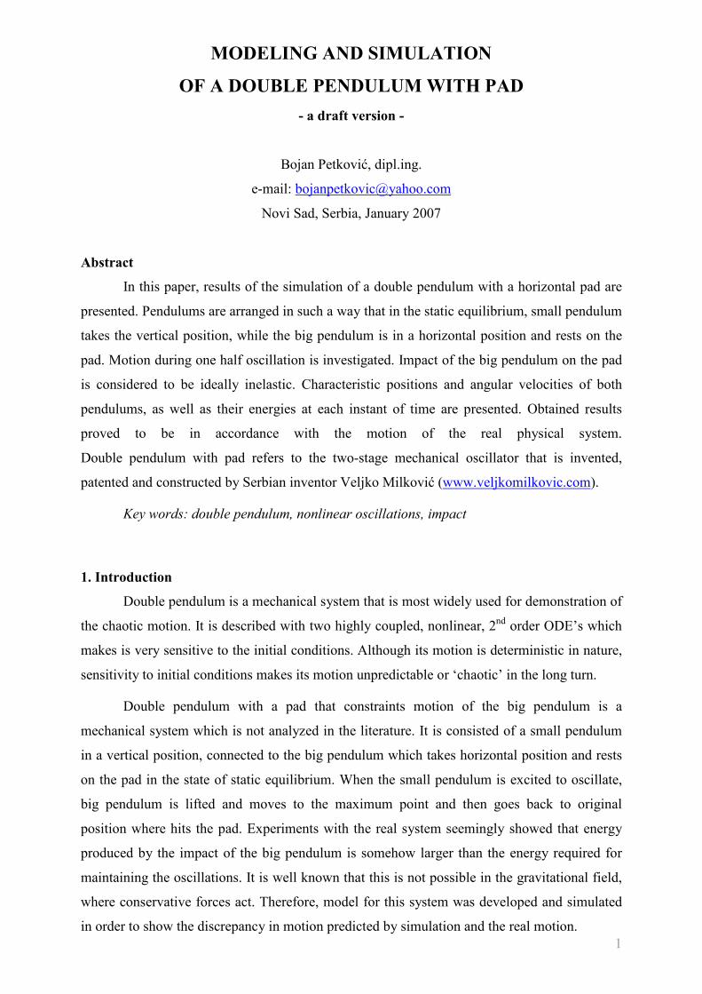
Double pendulum with pad is shown in Fig.1. System consists of: (i) the big pendulum

(K2) which can rotate around its axis (O2) attached to the construction support, (ii) the small

pendulum (K2) with its axis on the big pendulum (O1) and (iii) the horizontal pad. In the state

of static equilibrium, small pendulum takes the vertical position ( 01 =θ ), and big pendulum

takes the horizontal position (2

2

πθ = , Fig. 1a) and rest on the pad.

Figure 1. Characteristic positions of the double pendulum with pad during one half oscillation

When small pendulum is taken out of the equilibrium position and released

( 00

11 <= θθ , Fig.1b) it starts its motion toward equilibrium position. Angle 1θ is being

increased (decreases in its absolute value) so that vertical component of the small pendulum

weight (G1,v, Fig.2) increases. At the same time, vertical component of the centrifugal force,

Fc,v, is increased. At the moment t1, sum of these two forces gives momentum 1

2

F

OM that is

equal to the momentum of the big pendulum 2

2

G

OM . In that instant, big pendulum is lifted of the

pad (Fig. 1c) and is being moved upward. After 01 =θ is reached, vertical forces of the small

pendulum are decreasing and big pendulum slows down reaching the maximum position in the

moment t2 (Fig.1d). Big pendulum starts moving downward while small pendulum is slowing

down. At the moment t3, big pendulum hits the pad (Fig.1e) and we assume ideally inelastic

impact there. At the moment t4, small pendulum reaches maximum position and stops (Fig. 1f).

Period from t0 to t4 is called one half-oscillation.


3

3. Mathematical models

One half-oscillation period can be divided into three characteristic periods: (i) t0 to t1,

only small pendulum is in motion, (ii) t1 to t3, the whole system is in motion and (iii) t3 do t4,

only small pendulum is in motion. Mathematical model of a single pendulum is needed for

periods (i) and (iii), double pendulum model is required for period (ii). It is also necessary to

know time instants t1 and t3 when motion is switched from single to double pendulum and vice

versa. From the condition that momentum of forces are equal 2

2

1

2

G

O

F MMO

= , time t1 is

determined. Condition απθ −= 22 (Fig.3) determines time of the impact t3. It is also

necessary to determine the change in angular velocity of the small pendulum due to the impact.

Time t4 , when the small pendulum stops is calculated from the condition that angular

velocity of the small pendulum is equal to zero.

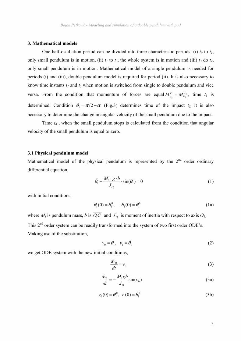
3.1 Physical pendulum model

Mathematical model of the physical pendulum is represented by the 2nd order ordinary

differential equation,

0)sin( 11

1

1

=⋅⋅⋅

+ θθOJ

bgM&& (1)

with initial conditions,

0

11

0

11 )0(,)0( θθθθ && == (1a)

where M1 is pendulum mass, b is 11CO and 1O

J is moment of inertia with respect to axis O1.

This 2nd order system can be readily transformed into the system of two first order ODE’s.

Making use of the substitution,

1110 , θθ &== vv (2)

we get ODE system with the new initial conditions,

10 v

dt

dv= (3)

)sin( 011

1

vJ

gbM

dt

dv

O

−= (3a)

0

11

0

10 )0(,)0( θθ &== vv (3b)


4

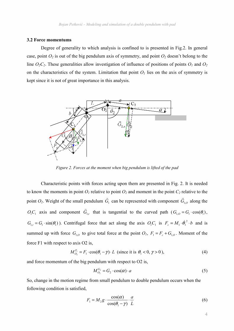
3.2 Force momentums

Degree of generality to which analysis is confined to is presented in Fig.2. In general

case, point O2 is out of the big pendulum axis of symmetry, and point O2 doesn’t belong to the

line O2C2. These generalities allow investigation of influence of positions of points O1 and O2

on the characteristics of the system. Limitation that point O1 lies on the axis of symmetry is

kept since it is not of great importance in this analysis.

Figure 2. Forces at the moment when big pendulum is lifted of the pad

Characteristic points with forces acting upon them are presented in Fig. 2. It is needed

to know the moments in point O1 relative to point O2 and moment in the point C2 relative to the

point O2. Weight of the small pendulum 1Gr

can be represented with component OG ,1

r along the

11CO axis and component tG ,1

r that is tangential to the curved path ( )cos( 11,1 θ⋅= GG O ,

)sin( 11,1 θ⋅= GG t ). Centrifugal force that act along the axis 11CO is bMFc ⋅⋅=2

11 θ& and is

summed up with force OG ,1 to give total force at the point O1, Oc GFF ,11 += . Moment of the

force F1 with respect to axis O2 is,

LFMF

O ⋅−⋅= )cos( 111

2γθ (since it is 0,01 >< γθ ), (4)

and force momentum of the big pendulum with respect to O2 is,

aGMG

O ⋅⋅= )cos(22

2α (5)

So, change in the motion regime from small pendulum to double pendulum occurs when the

following condition is satisfied,

L

agMF ⋅

−⋅=

)cos(

)cos(

1

21γθ

α (6)


5

Orientation of angles alfa and gama is denoted on the figure. Relations (4) and (5) are

indepenent of the 1θ , α or γ signs.

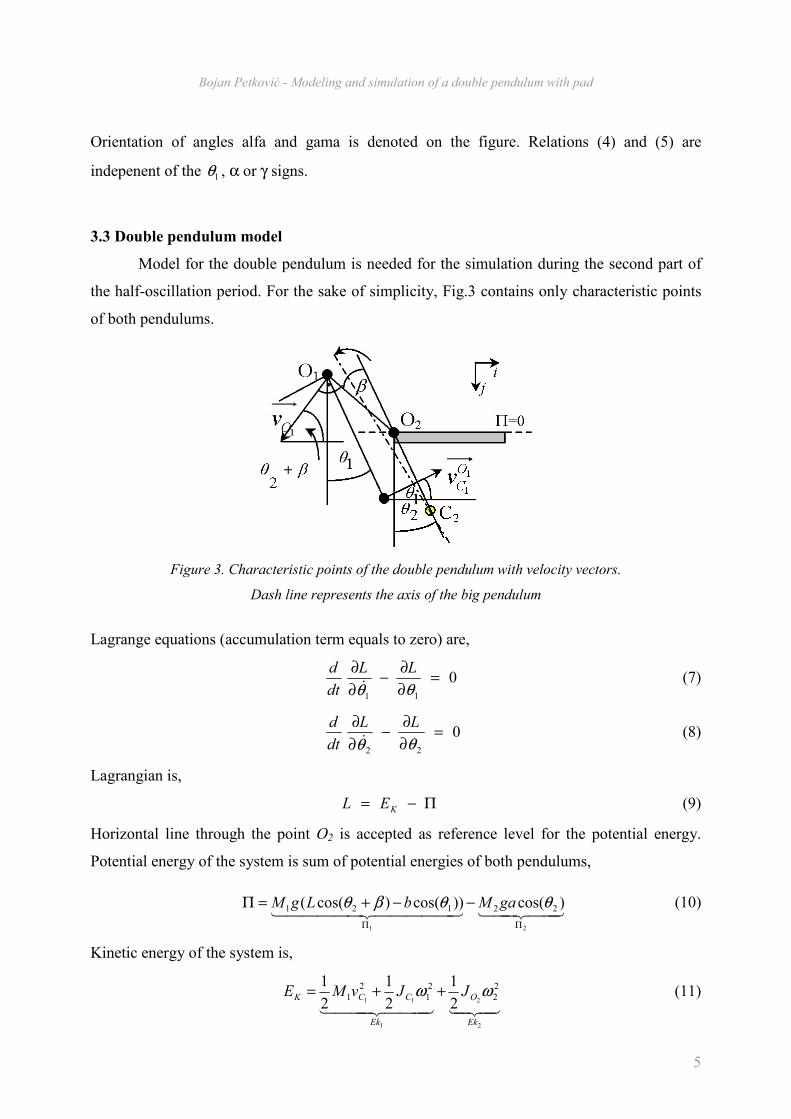
3.3 Double pendulum model

Model for the double pendulum is needed for the simulation during the second part of

the half-oscillation period. For the sake of simplicity, Fig.3 contains only characteristic points

of both pendulums.

Figure 3. Characteristic points of the double pendulum with velocity vectors.

Dash line represents the axis of the big pendulum

Lagrange equations (accumulation term equals to zero) are,

011

=∂

∂−

∂

∂

θθ

LL

dt

d&

(7)

022

=∂

∂−

∂

∂

θθ

LL

dt

d&

(8)

Lagrangian is,

Π−= KEL (9)

Horizontal line through the point O2 is accepted as reference level for the potential energy.

Potential energy of the system is sum of potential energies of both pendulums,

443442144444 344444 2121

)cos())cos()cos(( 22121

ΠΠ

−−+=Π θθβθ gaMbLgM (10)

Kinetic energy of the system is,

43421444 3444 212

2

1

11

2

2

2

1

2

12

1

2

1

2

1

Ek

O

Ek

CCK JJvME ωω ++= (11)


6

where 1C

J is the small pendulum moment of inertia with relation to point C1 and 2O

J is the big

pendulum moment of inertia with respect to O2. Velocity at the point C1 is the sum of two

velocities 1

111

O

COC vvv += ,

4444 34444 21444444 3444444 2111

1

1

1

1

1

111)sin()cos()sin()cos( 1122

OC

O v

O

C

O

C

v

OOC jvivjvivv ⋅−⋅+⋅++⋅+−= θθβθβθ . (12)

After introducing 21θ&LvO = and 1

1

1θ&bv

O

C = we get,

))sin()sin(())cos()cos(( 112211221θθβθθθθβθθ &&&& bLjbLivC −+⋅+++−⋅= (13)

)sin()sin(2)(sin)(sin

)cos()cos(2)(cos)(cos

21211

22

1

2

2

22

2

2

21211

22

1

2

2

22

2

22

1

βθθθθθθβθθ

βθθθθθθβθθ

+−+++

++−++=

&&&&

&&&&

LbbL

LbbLvC (14)

))(cos(2 2121

2

1

22

2

22

1βθθθθθθ +−−+= &&&& LbbLvC (15)

Using relations 11 θω &= , 22 θω &= and the expression for moment of inertia 2

222aMJJ CO += we

get the expression for the kinetic energy,

2

2

2

2

2

12121

2

1

22

2

2

1 )(2

1

2

1)))(cos(2(

2

121

θθβθθθθθθ &&&&&& aMJJLbbLME CCK ++++−−+= (16)

After introducing expressions for Ek i Π in Lagrangian, we have,

[ ])cos())cos()cos((

)(cos(2)()(2

1

22121

21211

2

21

22

21

2

1 21

θθβθ

βθθθθθθ

gaMbLgM

LbMaMJMLJbML CC

+−+−

−+−−++++= &&&& (17)

Partial derivatives in the Lagrangian are,

))(cos()( 2121

2

11

11

βθθθθθ

+−−+=∂

∂ &&&

LbMJbML

C (18)

))(cos()( 2111

2

1

2

12

22

βθθθθθ

+−−++=∂

∂ &&&

LbMaMLMJL

C (19)

)sin()(sin( 1121211

1

θβθθθθθ

gbMLbML

−+−=∂

∂ && (20)

)sin()sin())(sin( 222121211

2

θβθβθθθθθ

gaMgLMLbML

−+++−−=∂

∂ && (21)

))(sin())(sin())(cos()(

)))((sin())(cos()(

211

2

2211212112

2

11

2121122112

2

11

1

1

1

βθθθβθθθθβθθθθ

θθβθθθβθθθθθ

+−−+−++−−+=

=−+−++−−+=∂

∂

LbMLbMLbMJbM

LbMLbMJbML

dt

d

C

C

&&&&&&&

&&&&&&&&

(22)


7

))(sin())(sin())(cos()(

)))((sin())(cos()(

21121211

2

12111

2

1

2

12

2121112111

2

1

2

12

2

2

2

βθθθθβθθθβθθθθ

θθβθθθβθθθθθ

+−−+−++−−++=

=−+−++−−++=∂

∂

LbMLbMLbMaMLMJ

LbMLbMaMLMJL

dt

d

C

C

&&&&&&&

&&&&&&&&

(23)

After using these expressions in the Lagrange equations, we get,

0sinsincos 11211

2

22112

2

11 1=++−−+−−+ )(θgbMβ))(θ(θLbMθβ))(θ(θLbMθ)bMJ(θ

CBBA

C 321321&

321&&

43421&& (24)

)sin(sinsincos 2122211

2

12111

2

2

2

12 1βθgLM)(θgaMβ))(θ(θLbMθβ))(θ(θLbMθ)aMLMJ(θ

FEBBD

C +−++−++−−++321321321

&321

&&444 3444 21

&&

(25)

Using the following expressions,

glMFgaMEaMLMC

JD

gbMCLbMBbMC

JA

1;

2;2

22

11

1;

1;2

11

==++=

==+=

(26)

equations become more readable,

A

θCθ

A

β)(θθBθ

A

β))(θ(θBθ

)1

sin(22

)21

sin(

221

cos

1−

+−+

+−= &&&&& (27)

D

θE

D

βθFθ

D

β)(θθBθ

D

β))(θ(θBθ

)2

sin()2

sin(21

)21

sin(

121

cos

2−

++

+−−

+−= &&&&& (28)

In terms of angular accelerations ( 1θ&& i 2θ&& ), these equations are linear and can be linearly

combined in the equations where each one of them shows up independently. Substituting

second equation into the first and first equation into the second, the following system is

obtained,

−+−+++−−

−⋅+−++−

−

+−−

=

)1

sin()21

cos()2

sin()21

cos()2

sin(

...22

)21

sin(212

))21

(2sin(2

)21

(2cos2

11

θCβ)(θθβθD

FBβ)(θθθ

D

EB

θβ)(θθBθβ)(θθ

D

B

β)(θθD

BA

θ

&&&&

(29)

+−−++−

−⋅+−−+−

+−−

=

)21

cos()1

sin()2

sin()2

sin(

...21

)21

sin(222

))21

(2sin(2

)21

(2cos2

12

β)(θθθA

CBβθFθE

θβ)(θθBθβ)(θθ

A

B

β)(θθA

BD

θ

&&&&

(30)

Using these expressions,

23,

22,

11,

10θθθθ && ==== uuuu (31)


8

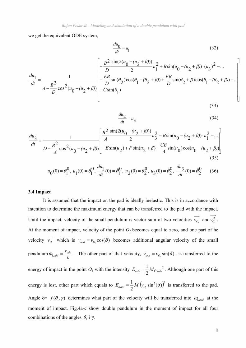
we get the equivalent ODE system,

10 u

dt

du= (32)

−

−+−+++−−

−⋅+−++−

−

+−−

=

)1

sin(

...)21

cos()2

sin()21

cos()2

sin(

...2)3

()20

sin(212

))20

(2sin(2

)20

(2cos2

11

θC

β)(θθβθD

FBβ)(θθθ

D

EB

uβ)(uuBuβ)(uu

D

B

β)(uuD

BA

dt

du

(33)

32 u

dt

du= (34)

+−−++−

−⋅+−−+−

+−−

=

)20

cos()0

sin()2

sin()2

sin(

...21

)20

sin(232

))20

(2sin(2

)20

(2cos2

13

β)(uuuA

CBβuFuE

uβ)(uuBuβ)(uu

A

B

β)(uuA

BD

dt

du

(35)

02

)0(3,02

)0(3

,02

)0(2

,01

)0(1,01

)0(1

,01

)0(0

θθθθθθ &&&&&& ======dt

duuu

dt

duuu (36)

3.4 Impact

It is assumed that the impact on the pad is ideally inelastic. This is in accordance with

intention to determine the maximum energy that can be transferred to the pad with the impact.

Until the impact, velocity of the small pendulum is vector sum of two velocities 1O

v and 1

1

O

Cv .

At the moment of impact, velocity of the point O1 becomes equal to zero, and one part of he

velocity 1O

v which is )cos(1

δOadd vv = becomes additional angular velocity of the small

pendulumb

vaddadd =,1ω . The other part of that velocity, )sin(

1δOaxis vv = , is transferred to the

energy of impact in the point O1 with the intensity 2

12

1axisaxis vME = . Although one part of this

energy is lost, other part which equals to ( )22

1 )(sin2

11

δOtrans vME = is transferred to the pad.

Angle δ= ),( 1 γθf determines what part of the velocity will be transferred into add,1ω at the

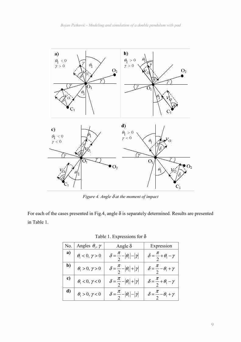
moment of impact. Fig.4a-c show double pendulum in the moment of impact for all four

combinations of the angles 1θ i γ.


9

Figure 4. Angle δ at the moment of impact

For each of the cases presented in Fig.4, angle δ is separately determined. Results are presented

in Table 1.

Table 1. Expressions for δ

No. Angles γθ ,1 Angle δ Expression

a) 0,01 >< γθ γθ

πδ −−= 1

2 γθ

πδ −+= 1

2

b) 0,01 >> γθ γθ

πδ +−= 1

2 γθ

πδ +−= 1

2

c) 0,01 << γθ γθ

πδ +−= 1

2 γθ

πδ −+= 1

2

d) 0,01 <> γθ γθ

πδ −−= 1

2 γθ

πδ +−= 1

2


10

4. Numerical procedure

General description of the numerical procedure follows. Code is given in the appendix.

1) Integrate ODE system for the small pendulum until the condition (6) is satisfied. It

is equivalent to the condition that vertical component of the force F1 is

L

agMF v ⋅⋅=

)cos(

)cos(2,1

γ

α. This condition is used for determination of the time instant

t1. Initial guess 00

1 =t ensures convergence.

2) Integrate ODE system for the double pendulum until big pendulum hits the pad.

Time instant t3 is determined from the condition απ

θ −=2

1 .

3) Determine new initial conditions for the small pendulum. Calculate energy of

impact as kinetic energy of the big pendulum plus transferred energy Etrans.

4) Integrate ODE system of the small pendulum until time t4 that is determined from

the condition 01 =ω .

Runge Kutta method of the 4th order with adaptive step size is used for integration of the ODE

system. Nonlinear equations were solved using Newton’s method.

5. Simulation results and discussion

Dimensions of the pendulums are given in Table 2. Material is iron of density 3/7860 mkg=ρ .

Table 2. Pendulum dimensions, moments of inertia

x [m] y [m] z [m] Mass [kg] CJ [kg⋅m2

]

K1 0.3 0.08 0.05 7.546 0.061

K2 0.6 0.1 0.05 23.58 0.727

Initial conditions used are 0,90,60 0,20,10,20,1 ===−= ωωθθ oo , oo 0,0 == γα

Table 3. Results

tmax Eimpact Etot,before Etot,after

0.488s 0.123J -9.253J -9.308J

One half-oscillation takes around 0.5s.


11

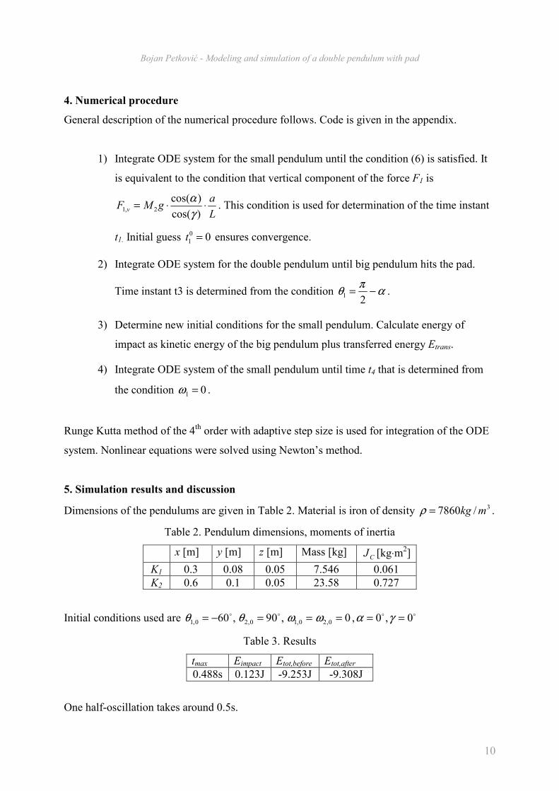
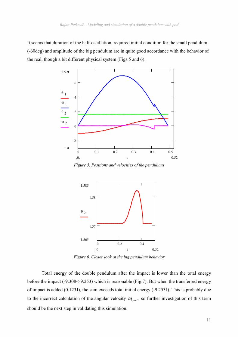
It seems that duration of the half-oscillation, required initial condition for the small pendulum

(-60deg) and amplitude of the big pendulum are in quite good accordance with the behavior of

the real, though a bit different physical system (Figs.5 and 6).

0 0.1 0.2 0.3 0.4 0.5

2

0

2

4

6

2.5 π⋅

π−

θ 1

ω 1

θ 2

ω 2

0.520 t

Figure 5. Positions and velocities of the pendulums

0 0.2 0.4

1.57

1.58

1.585

1.565

θ 2

0.520 t

Figure 6. Closer look at the big pendulum behavior

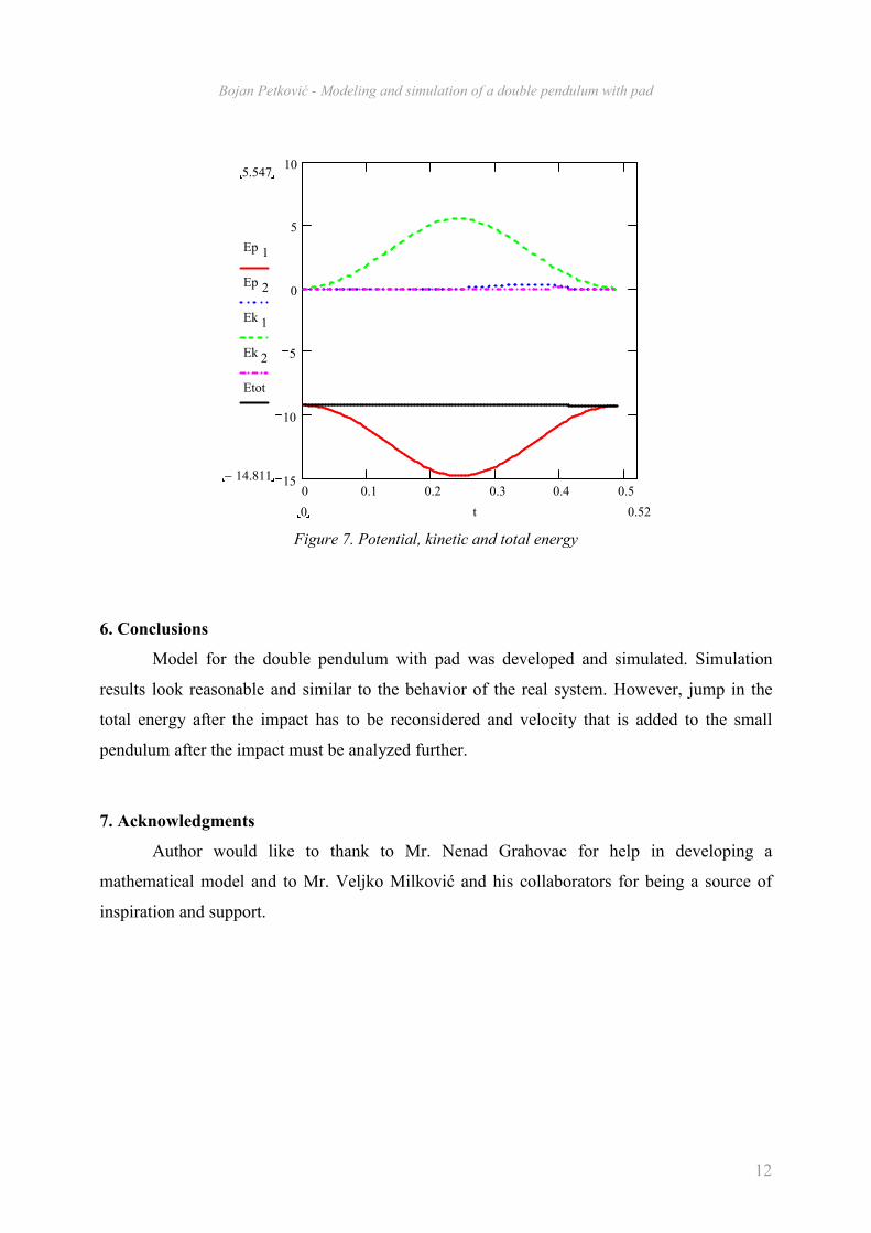
Total energy of the double pendulum after the impact is lower than the total energy

before the impact (-9.308<-9.253) which is reasonable (Fig.7). But when the transferred energy

of impact is added (0.123J), the sum exceeds total initial energy (-9.253J). This is probably due

to the incorrect calculation of the angular velocity add,1ω , so further investigation of this term

should be the next step in validating this simulation.


12

0 0.1 0.2 0.3 0.4 0.515

10

5

0

5

105.547

14.811−

Ep 1

Ep 2

Ek 1

Ek 2

Etot

0.520 t

Figure 7. Potential, kinetic and total energy

6. Conclusions

Model for the double pendulum with pad was developed and simulated. Simulation

results look reasonable and similar to the behavior of the real system. However, jump in the

total energy after the impact has to be reconsidered and velocity that is added to the small

pendulum after the impact must be analyzed further.

7. Acknowledgments

Author would like to thank to Mr. Nenad Grahovac for help in developing a

mathematical model and to Mr. Veljko Milković and his collaborators for being a source of

inspiration and support.

Documents

Bojan Petkovic-Modeling and Simulation of a Double Pendulum With Pad