Boltzmann-type Equations and their Applications · Publicações Matemáticas Boltzmann-type Equations and their Applications Ricardo Alonso PUC-Rio 30o Colóquio Brasileiro de Matemática

Boltzmann-type Equations and their Applications

Publicações Matemáticas

Boltzmann-type Equations and their Applications

Ricardo Alonso

PUC-Rio

30o Colóquio Brasileiro de Matemática

Copyright 2015 by Ricardo Alonso

Impresso no Brasil / Printed in Brazil

Capa: Noni Geiger / Sérgio R. Vaz

30o Colóquio Brasileiro de Matemática

Aplicacoes Matematicas em Engenharia de Producao - Leonardo J. Lustosa

e Fernanda M. P. Raupp

Boltzmann-type Equations and their Applications - Ricardo Alonso

Dissipative Forces in Celestial Mechanics - Sylvio Ferraz-Mello, Clodoaldo

Grotta-Ragazzo e Lucas Ruiz dos Santos

Economic Models and Mean-Field Games Theory - Diogo A. Gomes, Levon

Nurbekyan and Edgard A. Pimentel

Generic Linear Recurrent Sequences and Related Topics - Letterio Gatto

Geração de Malhas por Refinamento de Delaunay - Afonso P. Neto,

Marcelo F. Siqueira e Paulo A. Pagliosa

Global and Local Aspects of Levi-flat Hypersurfaces - Arturo Fernández

Pérez e Jiri Lebl

Introducao as Curvas Elipticas e Aplicacoes - Parham Salehyan

Métodos de Descida em Otimização Multiobjetivo - B. F. Svaiter e L. M.

Grana Drummond

Modern Theory of Nonlinear Elliptic PDE - Boyan Slavchev Sirakov

Novel Regularization Methods for Ill-posed Problems in Hilbert and Banach

Spaces - Ismael R. Bleyer e Antonio Leitão

Probabilistic and Statistical Tools for Modeling Time Series - Paul Doukhan

Tópicos da Teoria dos Jogos em Computação - O. Lee, F. K. Miyazawa, R.

C. S. Schouery e E. C. Xavier

Topics in Spectral Theory - Carlos Tomei

ISBN: 978-85-244-0401-6

Distribuição: IMPA

Estrada Dona Castorina, 110 22460-320 Rio de Janeiro, RJ

E-mail: [email protected]

http://www.impa.br

ii

“Alonso˙kinetic” — 2015/5/11 — 12:43 — page 3 — #3 ii

ii

ii

Contents

1 Introduction 5

2 From particle systems to kinetic models 72.1 Formal derivation of a mean field . . . . . . . . . . . . 82.2 Rigorous derivation of a mean field . . . . . . . . . . . 12

3 Classical Boltzmann equation 173.1 Well-posedness. Method of Kaniel & Shinbrot . . . . . 213.2 The method of DiPerna & Lions . . . . . . . . . . . . 26

3.2.1 Velocity average . . . . . . . . . . . . . . . . . 263.2.2 Renormalized solutions . . . . . . . . . . . . . 30

3.3 Theory of moments . . . . . . . . . . . . . . . . . . . . 383.4 Propagation of regularity . . . . . . . . . . . . . . . . 44

3.4.1 Step 1. Lp-bounds for Q+ . . . . . . . . . . . . 453.4.2 Step 2. Sharp lower bound for Q− . . . . . . . 483.4.3 Step 3. Gain of integrability of Q+ . . . . . . . 503.4.4 Step 4. Propagation of Sobolev regularity . . . 57

3.5 Entropy dissipation method and time asymptotic . . . 603.5.1 Relaxation of the linear Boltzmann model . . . 62

3.6 More on the Cauchy theory for Boltzmann . . . . . . . 68

4 Dissipative Boltzmann equation 694.1 Cucker-Smale model and self organization . . . . . . . 694.2 Modeling a granular material using Boltzmann equation 764.3 Rescaled problem and self-similar profile . . . . . . . . 804.4 1-D inelastic Boltzmann . . . . . . . . . . . . . . . . . 83

3

ii


ii

ii

4 CONTENTS

5 Radiative transfer equation 895.1 Scattering operator as a fractional diffusion . . . . . . 925.2 Regularization mechanism of the RTE . . . . . . . . . 965.3 On the Cauchy problem for singular scattering . . . . 101

6 Appendix 102

ii


ii

ii

Chapter 1

Introduction

Modern Kinetic theory is full of applications not only for the un-derstanding of complex phenomena but also for the development ofaccurate numerical schemes to resolve partial differential equationsin many areas. Let us cite for instance applications in semiconduc-tor modeling, radiative transfer, grain and polymer flows, biologicalsystems, cellular mechanics, chain supply dynamics, quantitative fi-nance, traffic models, wave propagation in random media, hydrody-namic and quantum models, understanding of boundary and inter-action in multi-scale phenomena, and phase transitions. The maingoal of this notes is precisely to present the reader an introduction tomodern kinetic theory. We will cover some of the influential result inthe area and give a baseline for research initiation in this topic leav-ing, of course, many important results out due to space and time.The list of reference is, by no means, exhaustive, yet, it is a goodinitial step for further reading and cross–reference.

These notes are divided in five chapters: Introduction, derivationof kinetic models from particle dynamics, classical Boltzmann equa-tion, dissipative Boltzmann equation and radiative transfer equation.After this introduction, we start covering basic ideas that help to un-derstand the kinetic modeling point of view. This translates math-ematically in the rigorous derivation of kinetic models from systemsof many particles. In some cases this process of going from particlesto kinetics is known as mean field limit. The third chapter begins by

5

ii


ii

ii

6 [CHAP. 1: INTRODUCTION

covering elementary material about the Boltzmann equation such asphysical interpretation, weak formulation, conservation laws and dis-sipation of entropy. It continues with a presentation of the classicaltheory of existence and uniqueness of weak solutions for the inhomo-geneous Boltzmann equation given by Kaniel & Shinbrot and a shortdiscussion of the celebrated theory introduced by DiPerna & Lionsof renormalized solutions. After covering the basic material, the sec-tion moves to the homogeneous Boltzmann equation explaining theimportance of the analysis of moments, propagation of integrabilityand regularity in the study of the equation. This section ends witha discussion on entropic methods and includes a short discussion ofthe celebrated result by Toscanni & Villanni on dissipation of en-tropy and its impact on the analysis for the long time asymptoticof the Boltzmann model. The fourth chapter will cover several rele-vant mathematical and physical aspects in the theory of viscoelasticmaterials modeled using the dissipative Boltzmann equation. Re-cent results on existence and uniqueness of solutions will be givenby revisiting the Kaniel & Shinbrot method adding a short discus-sion on the discrepancies and difficulties with respect to the classicalBoltzmann theory. Interesting phenomena present in dissipative dy-namics such as self-similar profiles, overpopulated tails, intermediateasymptotic properties, propagation of regularity and Haff’s law willbe commented (all of them inexistent in the classical elastic theory!).Several examples of dissipative kinetic models will be given in thissection mainly oriented to applications in biology and economics, suchas the celebrated Cucker & Smale model, wealth distribution modeland rod alignment model. The latter two fall directly in the the-ory of dissipative Boltzmann equation in one dimension. The notesends with a chapter devoted to the study of the radiative transportequation. Classical theory on integrable scattering and recent resultson the forward-peaked regime are presented. This equation will beused to motivate the theory of hypo-elliptic operators and fractionaldiffusions in mathematical physics.

ii


ii

ii

Chapter 2

From particle systemsto kinetic models

We start this notes with a generic example of a particle systemthat is widely used in physics, biomechanics, biology, economy, mate-rial sciences, traffic modeling and many other areas. The idea is sim-ple and comes from elementary mechanics: in a system of large num-ber of particles, particles essentially interact continuously by meansof friction and elasticity. These interactions are of different nature,interaction by friction produces loss of mechanical energy while elas-ticity is related to storage of mechanic energy due to deformation.This is a generic model in material science, a typical example is theKelvin–Voigt model for viscoelastic materials (viscosity and frictionare equivalent terms here). Assume we have a system with N par-ticles having position and velocity (xi, vi), the model that we brieflystudy in this section is given by the ODE system

dxidt

= vi ,dvidt

=1

N

∑j 6=i

Uf(|xj − xi|

)(vj − vi

)+

1

N

∑j 6=i

U ′e(|xj − xi|

)(xj − xi

).

(2.1)

Here Uf and Ue are the frictional and elastic potentials respectivelythat we consider depending only on the distance between particles. A

7

ii


ii

ii

8 [CHAP. 2: FROM PARTICLE SYSTEMS TO KINETIC MODELS

typical elastic potential is given by Ue(s) = κ2 s

2 which gives Hooke’slaw (linear law) in elasticity. A possible interpretation of model (2.1)is that a given particle experiments a weighted averaged frictionaland elastic forces due to interaction with other particles, that is,each particle experiments a mean field interaction. These averagesare presumably more influenced by close neighbors, thus, one expectssuch potentials to decay. Of course, the properties of the potentials,such as decay and smoothness, will completely determine the behav-ior of the system and the physics it models. Thus, it is natural toexpect that the mathematical analysis will be highly dependent onthe properties assumed for the potentials. For example, we refer to[7] for a numerical study of model (2.1) applied to cellular mechanics.

Before entering in mathematical details, let us formally discussa particular case of (2.1), the celebrated model in animal behaviorproposed by Cucker-Smale [36] which was first studied with mathe-matical rigor in [49]. The Cucker-Smale model is precisely the model(2.1) with zero elastic potential and frictional potential Uf ≥ 0 en-joying certain properties.

2.1 Formal derivation of a mean field

The goal in this short discussion is to derive a kinetic model (meanfiled model) for the particle model (2.1). Although this discussionis formal, it will help to introduce key ideas and concepts in kinetictheory that can be made rigorous in many instances. We start recall-ing that a Hamiltonian system is one that is completely described bya scalar function H(t,x,v), the Hamiltonian. The evolution of thesystem is given by

dx

dt= ∂vH

dv

dt= −∂xH ,

where x =(x1, · · · , xN

)and v =

(v1, · · · , vN

)are the vectors of po-

sitions and velocities of the particles respectively. The product space(x,v) is addressed as phase space. Many systems are Hamiltonian,including (2.1). There is a central result for Hamiltonian systemsdue to J. Gibbs: The distribution function of a Hamiltonian parti-cle system is constant along any trajectory in phase space. Indeed,

ii


ii

ii

[SEC. 2.1: FORMAL DERIVATION OF A MEAN FIELD 9

assume that the number of particles is large enough that it becomesmeaningful to observe the N -particle density distribution

fN (t,x,v) =number of particles at (t,x,v)

volume in phase space.

If J is the flux of particles at any given point of phase space, one hasfor any measurable set A

Variation number particles in A =d

dt

∫A

fN (t,x,v)dV(x,v)

=

∫∂A

J (t,x,v) · n dS(x,v) = Net flux through ∂A .

Using the divergence theorem∫∂A

J (t,x,v) · n dS(x,v) = −∫A

∇ · J (t,x,v)dV(x,v) .

It readily follows that∫A

(∂tf

N (t,x,v) +∇ · J (t,x,v))

dV(x,v) = 0 .

Two points are made here: (1) The measurable set A is arbitrary,and (2) the flux is related to the density distribution by the formula

J (t,x,v) = fN (t,x,v)d

dt

(x,v

).

One concludes that

0 = ∂tfN (t,x,v) +∇ · J (t,x,v)

= ∂tfN (t,x,v)+

d

dt

(x,v

)· ∇fN (t,x,v) +

(∇ · d

dt

(x,v

))fN (t,x,v) .

Observe that for the latter term

∇ · ddt

(x,v

)= ∇ ·

(∂vH,−∂xH

)= ∂x∂vH− ∂v∂xH = 0 .

ii


ii

ii


The conclusion is an equation known as Liouville’s equation

∂tfN (t,x,v) +

d

dt

(x,v

)· ∇fN (t,x,v) = 0 , (2.2)

which is precisely Gibbs’ statement. Now, Gibbs’ statement is aboutthe N -particle distribution function, what we really want is a closedequation for the single distribution function

f(t, x1, v1) :=

∫fN (t,x,v)dV N−1(x,v) ,

where the superscript N − 1 is added to the differential to denotean integration on the last N − 1 coordinates (xi, vi) of the phasespace. Since particles are indistinguishable, it is irrelevant which sin-gle density distribution we choose to describe. Of course, in a generalsituation finding a closed equation for the single particle distributionis an impossible task because particle trajectories are necessarily cor-related (particles are interacting at all times), so any mathematicalformalism will include dependence of all particles. However, it is pos-sible to argue that in a situation of a large number of particles, onemay find a good approximating model for the evolution of the singleparticle distribution. The argument goes like this for the Cucker-Smale model: Note that Liouville’s equation in such case reduces to

∂tfN +

∑i

vi · ∇xifN +1

N

∑i

∇vi ·(∑

j

Uf(|xi−xj |

)(vj − vi

)fN).

(2.3)Integrate equation (2.3) in (x,v)N−1 and observe that the divergencetheorem leads to

∫ ∑i

vi · ∇xifN dV N−1(x,v) = v1 · ∇x1f(t, x1, v1) .

ii


ii

ii

[SEC. 2.1: FORMAL DERIVATION OF A MEAN FIELD 11

Additionally,

1

N

∑i

∫∇vi ·

(∑j

Uf(|xi − xj |

)(vj − vi

)fN)dV N−1(x,v)

=1

N

∫∇v1 ·

( N∑j=2

Uf(|x1 − xj |

)(vj − v1

)fN)dV N−1(x,v)

=N − 1

N

∫∇v1 ·

(Uf(|x1 − x2|

)(v2 − v1

)fN)dV N−1(x,v)

=N − 1

N

∫∇v1 ·

(Uf(|x1 − x2|

)(v2 − v1

)f2)

dx2dv2 .

In the first equality we used divergence theorem which vanishes thelast N − 1 terms of the outer sum. In the second equality we usedsymmetry of fN (particles are indistinguishable), thus, the interac-tion between particles (1, j) equals N − 1 times the interaction ofparticles (1, 2). And, for the last equality we used the obvious def-inition of the two-particle distribution function f2. Now, a centralissue rises here and it is known as molecular chaos. That is to say,for large number of particles

f2(t, x1, v1, x2, v2) ≈ f(t, x1, v1) f(t, x2, v2) . (2.4)

This means that the specific position and velocity of one particularparticle is almost uncorrelated, at any time, to the specific positionand velocity of any other particle. Intuitively this should be the casefor particles that follow the mean field of particles rather than a sin-gle one such us model (2.1). Molecular chaos should also holds insystems such as billiards (related to the Boltzmann equation) wheretwo particles bear large number of interactions in between their par-ticular interaction. That is, at the moment of their interaction suchparticles are essentially uncorrelated.

This argument leads to the approximated closed equation

∂tf(t, x, v) + v · ∇xf(t, x, v)

+ N−1N ∇vf(t, x, v) ·

∫Uf(|x∗ − x|

)(v∗ − v

)f(t, x∗, v∗) dx∗dv∗ ≈ 0 ,

valid for large number of particles N . In the limit N → ∞ themolecular chaos approximation (2.4) should become exact, thus, if

ii


ii

ii


the distribution sequence f := fN converges, say to f , one finds thekinetic description (mean field limit) of the Cucker-Smale particlemodel

∂tf + v · ∇xf +∇v ·Q(f, f) = 0 , (2.5)

where,

Q(f, f)(t, x, v) := f(t, x, v)

∫Uf(|x∗−x|

)(v∗−v

)f(t, x∗, v∗) dx∗dv∗ .

(2.6)

2.2 Rigorous derivation of a mean field

Let us give now a rigorous treatment of the mean field limit givenin previous discussion for a particle model slightly more general that(2.1). We add some random fluctuations to the particles and per-form the analysis following the program proposed in [70, 26]. Thus,consider a large system of N -interacting particles having positions(xi(t), vi(t)) ∈ R2d and following the dynamics

dxi(t) = vi(t)dt , dvi(t) =√

2 dBi(t)

− 1

N

∑j 6=i

H(xi(t)− xj(t), vi(t)− vj(t)

)dt ,

(2.7)

with independent initial data (xi(0), vi(0)) all having the same distri-bution law fo. The processes Bi(t) are independent standard brow-nian motions in Rd. The interacting potential H : R2d → Rd isassumed to be Lipschitz continuous.

The central analytical result consists in proving that such process(xi(t), vi(t)) behave in the limit N → ∞ like a process (xi(t), vi(t))solving the McKean-Vlasov equation on R2d

dxi(t) = vi(t)dt , dvi(t) =√

2 dBi(t)−(H ∗ f

)(t, xi(t), vi(t))dt ,

(2.8)where the initial condition is given by (xi(0), vi(0)) = (xi(0), vi(0))and f(t, x, v) is the law of (xi(t), vi(t)). It is well know from the theoryof Ito processes that the law of (xi, vi(t)) satisfies the KolmogorovForward equation, see for instance the tutorial [64]

∂tf + v · ∇xf = ∆vf +∇ ·(f(H ∗ f

)), f(0) = fo . (2.9)

ii


ii

ii

[SEC. 2.2: RIGOROUS DERIVATION OF A MEAN FIELD 13

We refer to [26, Theorem 1.2] for a complete proof about existence anduniqueness of systems (2.7) and (2.8) under suitable conditions on theinitial law fo. In particular, the fact that equation (2.9) have uniquesolution implies that all processes are equally distributed which ex-plain why we dropped the index in the law f := fi. One fact thatholds for solutions f of equation (2.9), which we will need below, isthat spatial and velocity moments of order two are propagated, inorder words∫R2d

(|x|2+|v|2

)dfo(x, v) −→ sup

t∈[0,T ]

∫R2d

(|x|2+|v|2

)df(t, x, v) ≤ CT .

(2.10)

Theorem 2.2.1. Let fo be a Borel probability measure having spatialand velocity moments of order two, and the initial state (xi(0), vi(0))be independent random variables with common law fo. Under theaforementioned conditions, there exists a constant CT such that

supt∈[0,T ]

max0≤i≤N

(E[|xi(t)− xi(t)|2

]+ E

[|vi(t)− vi(t)|2

])= supt∈[0,T ]

(E[|x1(t)− x1(t)|2

]+ E

[|v1(t)− v1(t)|2

])≤ CT

N.

Proof. Define the fluctuations xei (t) := xi(t) − xi(t) and vei (t) :=vi(t)− vi(t) for i = 1, · · · , N and introduce the total error

e(t) = max1≤i≤N

{E[|xei (t)|2 + |vei (t)|2

]}.

Now, subtract the models (2.7) and (2.8). Thus, for the positionfluctuations one has

1

2

d

dtE[|xei (t)|2

]= E

[xei (t) · vei (t)

]≤ e(t)

2. (2.11)

The velocity fluctuations require more work. One certainly has thatthe velocity fluctuations satisfy

1

2

d

dtE[|vei (t)|2

]= − 1

N

∑j 6=i

E[vei (t) ·

(H(xi(t)− xj(t), vi(t)− vj(t))

−(H ∗ f

)(t, xi(t), vi(t))

)]=: I1 + I2 ,

(2.12)

ii


ii

ii


where (dropping the t variable to ease notation)

I1 = − 1

N

∑j 6=i

E[vei ·

(H(xi − xj , vi − vj)−H(xi − xj , vi − vj)

)]and,

I2 = − 1

NE[vei ·

∑j 6=i

(H(xi − xj , vi − vj)−

(H ∗ f

)(t, xi, vi)

)]=: − 1

NE[vei ·

∑j 6=i

Yi,j

].

The term I1 is controlled using Lipschitz continuity of H∣∣∣H(xi − xj , vi − vj)−H(xi − xj , vi − vj)∣∣∣

≤ ‖H‖Lip(|xei |+ |vei |+ |xej |+ |vej |

),

as a consequence, a simple application of Young’s inequality leads to∣∣I1(t)∣∣ ≤ 5

2‖H‖Lip e(t) . (2.13)

For the term I2 one has∣∣I2∣∣ ≤ 1

N

√E[|vei |2

]√E[∣∣∣∑

j 6=i

Yi,j

∣∣∣2] .Furthermore, for any j 6= k

E[Y i,j · Y i,k

]= E

[E[Y i,j · Y i,k

∣∣(xi, vi)]]= E

[E[Y i,j

∣∣(xi, vi)] · E[Y i,k∣∣(xi, vi)]]since processes (xj(t), vj(t)) are uncorrelated. A direct computationshows then

E[Y i,j

∣∣(xi, vi)]=

∫R2d

(H(xi − x∗, vi − v∗)−

(H ∗ f

)(t, xi, vi)

)df(t, x∗, v∗)

= (H ∗ f)(t, xi, vi)− (H ∗ f

)(t, xi, vi) = 0 .

ii


ii

ii

[SEC. 2.2: RIGOROUS DERIVATION OF A MEAN FIELD 15

Here we have use that the law of (xj(t), vj(t)) is precisely f(t). There-fore,

E[∣∣∣∑

j 6=i

Yi,j

∣∣∣2] = (N − 1)E[∣∣Y1,2∣∣2]

≤ (N − 1)

∫R4d

∣∣H(x− x∗, v − v∗)∣∣2df(t, x, v)df(t, x∗, v∗)

≤ 4(N − 1)

∫R4d

(‖H‖2Lip

(∣∣x− x∗∣∣2 +∣∣v − v∗∣∣2)

+∣∣H(0, 0)

∣∣2)df(t, x, v)df(t, x∗, v∗) ≤ CT (N − 1) ,

where in the last inequality we used (2.10). In summary,

∣∣I2(t)∣∣ ≤ CT√e(t)√

N≤ e(t) +

CTN

. (2.14)

Gathering (2.11), (2.12), (2.13) and (2.14) one gets

E[|xei (t)|2

]+ E

[|vei (t)|2

]≤ co

∫ t

0

e(s)ds +CTN

, 1 ≤ i ≤ N . (2.15)

Here co is independent of T > 0. Since the right side of (2.15) isindependent of the particle i, we can compute the max along theparticles and use Gronwall’s lemma to conclude

supt∈[0,T ]

e(t) ≤ CTcoN

ecoT .

The proof is concluded by noticing that all single marginals of thejoin probability of N–particles are equal because particles are indis-tinguishable. Thus,

e(t) = E[|x1(t)− x1(t)|2 + |v1(t)− v1(t)|2

].

Convergence in mean square implies convergence in probability.Thus, Theorem 2.2.1 readily implies that lim

N→∞f1N (t) = f(t), where

ii


ii

ii


f1N (t) is the single marginal of the join probability of N -particles attime t. Furthermore, it also implies a precise quantitative version ofmolecular chaos. In order to see this, let us introduce the Wassersteindistance between Borel probability measures (µ, ν), see for instance[73], as

d2(µ, ν) = inf(X,Y )

√E[|X − Y |2

], (2.16)

where the infimum is taken over all couples of random variable (X,Y )with X having law µ and Y having law ν. Thus,

supt∈[0,T ]

d2(f1N (t), f(t))2

≤ E[∣∣(x1(t), v1(t))− (x1(t), v1(t))

∣∣2]= E

[|x1(t)− x1(t)|2 + |v1(t)− v1(t)|2

]≤ CT

N.

Moreover, the k-marginal fkN converges towards the tensor f⊗k as Nincreases since

supt∈[0,T ]

d2(fkN (t), f⊗k(t))2

≤ E[∣∣(x1(t), v1(t), · · · , xk(t), vk(t))− (x1(t), v1(t), · · · , xk(t), vk(t))

∣∣2]= kE

[|x1(t)− x1(t)|2 + |v1(t)− v1(t)|2

]≤ k CT

N.

ii


ii

ii

Chapter 3

Classical Boltzmannequation

We saw in the previous section that the mean field limit of parti-cle systems interacting with smooth potentials is given by integro–differential equations. Solutions of such equations are interpretedas distributions of particles depending on space x (macroscopic vari-able), velocity v (microscopic or kinetic variable) and time t (which is,somehow, both a macro and a micro variable). The Boltzmann equa-tion is also an integro–differential equation that represents the kineticdescription of a many–particle system interacting through collisions.Such interaction is of different nature to that of friction or elasticity:a collision is a discontinuous process while interactions with smoothpotentials is continuous. This seemingly banal difference proves tobe crucial in the rigorous derivation of the Boltzmann model fromparticle dynamics. In fact, such derivation is still an open (and quiteimportant) problem in statistical physics. Let us write down themodel and try to explain it, at least, at the formal level

∂tf + v · ∇xf = Q(f, f) , (t, x, v) ∈ R+ × R2d , (3.1)

complemented with an initial configuration f(0) = fo. Here the op-erator Q(f, f) will represent collision interactions between particles.More specifically, its bilinear form is defined, for any suitable func-

17

ii


ii

ii

18 [CHAP. 3: CLASSICAL BOLTZMANN EQUATION

tions f and g, as

Q(f, g)(v) :=∫Rd

∫Sd−1

(f(′v)g(′v∗)− f(v)g(v∗)

)B(v − v∗, ω)dωdv∗ .

(3.2)

We need to do some explaining with the introduced notation. Thepair (v, v∗) represents velocities of two particles that just collide andhad, before collision, velocities ′v and ′v∗. In this way, the pair (′v,′v∗)are pre-collisional velocities. Similar, it is common the notation(v′, v′∗) to represent post-collisional velocities of a pair of particleshaving velocities v and v∗ before collision. In the classical Boltz-mann equation the collision law map Cω : (v, v∗) → (v′, v′∗) is veryspecial because must conserve microscopic momentum and energy, inother words, is such that

v′ + v′∗ = v + v∗ , |v′|2 + |v′∗|2 = |v|2 + |v∗|2 . (3.3)

One concludes that it must be the case that (see [34] or Lemma 3.0.2below)

v′ = v − (u · ω)ω , v′∗ = v∗ + (u · ω)ω , (3.4)

where ω represents the unit vector perpendicular to the collision planeand u := v − v∗ is the relative velocity between particles. Now,the function B ≥ 0 is commonly known as collision kernel and itdescribes the physics of the collision, we refer to [34] and [71] forextensive discussion. It is customary to assume the factorization inthe mathematics community

B(u, ω) = |u|γ b(u · ω) , γ ∈ (−d, 2] . (3.5)

It is understood that u = u/|u|. The function b is known as scatter-ing kernel and weights the probability of scattering at certain angleafter a collision event. It is customary to assume the so-called cutoffhypothesis ∫

Sd−1

b(u · ω)dω <∞ .

Although, cutoff is a realistic assumption, such hypothesis fails to betrue in some relevant physical situations. The last section of these

ii


ii

ii

19

notes is brought precisely to give an introduction to the mathematicaltheory when such hypothesis is not met. The most typical exampleof (3.5) is the so called hard-spheres model which describes the dy-namics of a 3-dimensional billiard and is given by B(u, ω) = |u · ω|which corresponds to γ = 1. Furthermore, in the mathematical lit-erature, the cases γ ∈ (−d, 0), γ = 0, and γ ∈ (0, 1] are addressed assoft potentials, Maxwell molecules and hard potentials respectively.Properties of the collision law map Cω are given in the followinglemma,

Lemma 3.0.2. For any ω ∈ Sd−1 it follows that: (1) Cω ◦ Cω = Id,(2) detCω = −1, (3) the only functions ϕ satisfying ϕ+ϕ∗ = ϕ′+ϕ′∗are given by

ϕ(v) = a+ b · v + c |v|2 , a, c ∈ R, b ∈ Rd .

Such functions are called collision invariants (here ϕ′ = ϕ(v′) andϕ′∗ = ϕ(v′∗)).

Proof. Let us denote the post-collisional relative velocity as u′ =v′−v′∗. Item (1) is clear since u′ ·ω = −u ·ω. A proof of (2) follows byintroducing the map Cω : (v, u) → (v′, u′). Clearly, detCω = detCω,moreover, the matrix representation for Cω is given by[

Cω]

=

[1 −ω ⊗ ω0 1− 2ω ⊗ ω

].

Thus, det Cω = det(1−2ω⊗ω

)= det

(diag(−1, 1, · · · , 1)

)= −1. For

a proof of item (3) see for instance [65].

Particles are continuously colliding, thus, one may think that theyare experiencing a birth-death process with respect to the velocityvariable: at time t two particles occupying the same spatial pointx will not longer have velocity (v, v∗) if they collide, that is, withapproximate probability

Prob. of death of a pair (v, v∗) ≈ f(t, x, v) f(t, x, v∗)B(u, ω)dωdv∗ .

Similarly, at time t two particles occupying the same spatial pointx will create two particles with velocities (v, v∗) if they just collidedhaving velocities (′v,′v∗), that is, with approximate probability

Prob. of birth of a pair (v, v∗) ≈ f(t, x,′v) f(t, x,′v∗)B(u, ω)dωdv∗ .

ii


ii

ii


The collision operator is just the integration of this probabilities overall possible collision directions ω and velocities v∗. Note, that we haveused propagation of chaos in computing these approximate probabili-ties, namely, the joint distribution of two particles is approximate theproduct of the single distributions. Intuitively, this should be veryaccurate since the velocity correlation between two particles is min-imal in a large system of them sustaining numerous collisions. Theproof of this fact is a notoriously difficult problem in the Boltzmanncontext. The reader can find a proof of the following proposition in[34, 65].

Proposition 3.0.3. For a B satisfying (3.5) one has the followingproperties:(1) (Conservation) For all suitable functions f and ϕ∫

RdQ(f, f)(v)ϕ(v)dv =

1

4

∫RdQ(f, f)(v)

(ϕ′ + ϕ′∗ − ϕ− ϕ∗

)dv

(2) (Boltzmann’s H-Theorem)∫RdQ(f, f)(v) ln(f(v)) dv ≤ 0 .

(3) (Gaussian equilibria) And, for any B > 0 one have the equivalence

Q(F, F ) = 0←→ F (v) :=ρ

(2πT )d/2e−|v−vo|2

2T .

for some ρ, T ≥ 0 and vo ∈ Rd.

Note that, thanks to Proposition 3.0.3, solutions of the Boltzmannequation formally satisfy

∫Rdf(v)

1v|v|2

dv = 0 . (3.6)

Proposition 3.0.3 also leads to an important observation. Introduce

ii


ii

ii

[SEC. 3.1: WELL-POSEDNESS. METHOD OF KANIEL & SHINBROT 21

the entropy and the dissipation of entropy as

H(f) : =

∫Rdf ln(f)dvdx ,

0 ≤ D(f) : =

1

4

∫R3d

∫Sd−1

(f ′f ′∗ − ff∗

)(ln(f ′f ′∗)− ln(ff∗)

)Bdωdv∗dvdx .

(3.7)

Note the the dissipation of entropy is nonnegative because the loga-rithm is an increasing function. Then, it follows that a solution f ofthe Boltzmann equation formally satisfy

∂tH(f) +D(f) = 0 . (3.8)

In other words, the entropy of our particle system does not increase,H(f) ≤ H(fo) .

3.1 Well-posedness. Method of Kaniel &Shinbrot

The theory of well-posedness for the Cauchy problem of the Boltz-mann equation for general data is incomplete despite the efforts ofthe mathematics community. However, in certain circumstances it ispossible to give a complete proof of existence and uniqueness of non-negative solutions. One of the most celebrated methods, due to itssimplicity and beauty, is the Kaniel & Shinbrot iterations, see [53],which we present here. This method can be used for short time exis-tence with general initial data and for global well-posedness in someperturbative regimes. We sketch the latter by following the papers[51, 12]. First note that, under Grad cutoff assumption, the collisionoperator splits naturally in a gain and loss part (corresponding thethe birth and death process respectively)

Q(f, f) = Q+(f, f)−Q−(f, f) .

Second, obseve that using characteristics f#(t, x, v) := f(t, x+ tv, v)it is possible to write the Boltzmann equation as

df#

dt+Q#

−(f, f) = Q#+(f, f) . (3.9)

ii


ii

ii


Now, for simplicity assume the factorization of the scattering kernel(3.5). Then, it follows that the loss part of the collision operatorreduces to

Q−(f, f)(v) = f(v)

∫Rdf(v∗)

∣∣v − v∗∣∣γdv∗ =: f(v)R(f)(v).

Thus, integrating equation (3.9) follows that a solution of the Boltz-mann equation satisfies the relation

f#(t, x, v) = e−∫ t0R#(f)(s,x,v)dsfo(x, v)

+

∫ t

0

e−∫ tsR#(f)(τ,x,v)dτQ#

+(f, f)(s, x, v)ds .(3.10)

Finally, introduce the Banach space M of functions with Gaussian(or Maxwellian) decay in space-velocity with norm

‖g‖M =∥∥g e|x|2+|v|2∥∥∞ .

With these notations and definitions, we are ready to proceed andgive a well-posedness result for the Boltzmann equation in the so-called near vacuum regime, that is, when the initial data is sufficientlysmall in M. The essence of the method consist in defining the fol-lowing nested sequences of functions {ln} and {un} as solutions ofthe linear problems

dl#ndt

+Q#−(ln, un−1) = Q#

+(ln−1, ln−1) and

du#ndt

+Q#−(un, ln−1) = Q#

+(un−1, un−1) ,

(3.11)

with the terms satisfying the initial condition 0 ≤ ln(0) ≤ fo ≤ un(0).The construction begins by choosing a pair (l0, u0) satisfying whatKaniel and Shinbrot called the beginning condition

0 ≤ l#0 ≤ l#1 ≤ u

#1 ≤ u

#0 ∈M . (3.12)

It is precisely in the beginning condition where the methods fails forgeneral initial data.

ii


ii

ii


Theorem 3.1.1. Assume Grad’s cut off and factorization (3.5) hy-potheses for the scattering kernel B. Assume also −(d− 1) < γ ≤ 1,and let {ln} and {un} be the sequences defined by the mild solutionsof the linear problems (3.11). In addition, assume that the beginningcondition (3.12) is satisfied. Then,

(i) The sequences {ln} and {un} are well defined for n ≥ 1. Inaddition, {ln}, {un} are increasing and decreasing sequencesrespectively, and

l#n ≤ u#n a.e.

(ii) There exists ε > 0 such that if

‖u#0 ‖M ≤ ε and , 0 ≤ ln(0) = fo = un(0) for n ≥ 1 ,

thenlimn→∞

ln = limn→∞

un = f a.e.

The nonnegative limit f ∈ C(0, T ;M), with T > 0, is theunique solution of the Boltzmann equation and fulfills

0 ≤ l#0 ≤ f# ≤ u#0 ∈M a.e.

Proof. Item (i) follows by induction where the beginning condition isexactly the first step of the induction. Assuming that {lk} and {uk}are increasing and decreasing respectively, and such that lk ≤ uk for1 ≤ k ≤ n − 1, we can prove that same holds for k = n. Indeed,integration of the linear system (3.11) give us

l#n (t) = e−∫ t0R#(un−1)(s)dsln(0)

+

∫ t

0

e−∫ tsR#(un−1)(τ)dτQ#

+(ln−1, ln−1)(s)ds

≤ e−∫ t0R#(ln−1)(s)dsun(0)

+

∫ t

0

e−∫ tsR#(un−1)(τ)dτQ#

+(un−1, un−1)(s)ds

= u#n (t) .

(3.13)

Same argument proves that l#n−1 ≤ l#n and u#n ≤ u#n−1. Let us present

a lemma that will help us to prove item (ii).

ii


ii

ii


Lemma 3.1.2. Assume −(d − 1) < γ ≤ 1. Then, for any 0 ≤s ≤ t and functions f#, g# that lie in L∞

([0, T );M

)the following

inequality holds∫ t

s

∣∣∣Q#+(f, g)(τ)

∣∣∣ dτ ≤Cd,γ e

−|x|2−|v|2 ∥∥f#∥∥L∞(0,T ;M)

∥∥g#∥∥L∞(0,T ;M)

,

(3.14)

where the constant Cd,γ depends only on the dimension and γ. Inother words, ∫ t

0

∣∣∣Q#+(f, g)(τ)

∣∣∣ dτ ∈M , t ≥ 0 .

Proof. An explicit calculation yields the inequality,∣∣∣Q#+(f, g)(τ, x, v)

∣∣∣ ≤ e−|v|2 ∥∥f#∥∥L∞(0,T ;M)

∥∥g#∥∥L∞(0,T ;M)

×∫Rde−|v∗|

2

∫Sd−1

e−|x+τ(v−′v)|2−|x+τ(v−′v∗)|2b(u · ω)dω |u|γdv∗.

(3.15)

Note that

|x+ τ(v −′v)|2 + |x+ τ(v −′v∗)|2

= |x|2 + |x+ τu|2 ,

and, ∫ t

s

e−|x+τu|2

dτ ≤∫ ∞−∞

e−|τu|2

dτ ≤√π |u|−1.

Therefore, integrating (3.15) in [s, t]∫ t

s

∣∣∣Q#+(f, g)(τ, x, v)

∣∣∣dτ ≤ √π exp(−|x|2 − |v|2

)∥∥f#∥∥

L∞(0,T ;M)

∥∥g#∥∥L∞(0,T ;M)

∫Rde−|v∗|

2

|u|γ−1dv∗.

Finally, the proof is completed by observing that,∫Rde−|v∗|

2

|u|γ−1dv∗ ≤∫{|v∗|<1}

|u|γ−1dv∗ +

∫{|v∗|≥1}

e−|v∗|2

dv∗

≤ |Sd−1|d+ γ − 1

+ Cd .

ii


ii

ii


Let us proceed to prove item (ii). Define δ#n = u#n − l#n , thus, sub-tracting equations (3.11) follows

dδ#ndt≤ Q#

+(δn−1, un−1) +Q#+(ln−1, δn−1) +Q#

−(ln, δn−1) . (3.16)

Integrating (3.16) in time, recalling that δ#n (0) = δn(0) = 0 and usingLemma 3.1.2, it follows that

δ#n (t) ≤ Cd,γ e−|x|2−|v|2×(

‖u#n−1‖L∞(M) + ‖l#n−1‖L∞(M) + ‖l#n ‖L∞(M)

)‖δ#n−1‖L∞(M)

≤ 3Cd,γ e−|x|2−|v|2‖u#0 ‖M‖δ

#n−1‖L∞(M) , t ≥ 0 .

(3.17)

The conclusion from (3.17) is that

‖δ#n ‖L∞(M) ≤ 3Cd,γ‖u#0 ‖M‖δ#n−1‖L∞(M) . (3.18)

Taking ε := 1/(4Cd,γ) it follows directly from (3.18) that

‖δ#n ‖L∞(M) ≤ (3/4)n−1‖δ#0 ‖L∞(M) ≤ (3/4)n‖u#0 ‖M ,

which proves (ii).

Theorem 3.1.3. (Well-posedness near vacuum) Let B be a scatter-ing kernel satisfying Grad’s cut off and the factorization (3.5) with−(d−1) < γ ≤ 1. Then, there exists εo > 0 such that if ‖fo‖M ≤ εo,the Cauchy-Boltzmann problem has a unique global solution f satis-fying the estimate ∥∥f#∥∥

L∞([0,T );M)≤ 2 εo , (3.19)

for any 0 ≤ T ≤ ∞.

Proof. The key step to apply Theorem 3.1.1 is to find suitable func-tions that satisfy the beginning condition globally. The most natural(and simplest) choice for the first terms of the nested sequences {ln}and {un} is

l#0 = 0 and u#0 = ε e−|x|2−|v|2 .

ii


ii

ii


Here ε > 0 is the parameter given in Theorem 3.1.1, item (ii). Nowcompute the following two terms

l#1 (t) = fo e−

∫ t0R#(u0)(τ)dτ and u#1 (t) = fo +

∫ t

0

Q#+(u0, u0)(τ)dτ.

Clearly, 0 ≤ l#0 ≤ l#1 ≤ u#1 . In addition, using Lemma 3.1.2 in the

expression for u#1 we conclude that, for all t ≥ 0,

u#1 (t) ≤(‖fo‖M + Cd,γ‖u#0 ‖2M

)e−|x|

2−|v|2 .

Noting that ‖u#0 ‖M = ε, it suffices to satisfy the inequality

‖fo‖M + Cd,γε2 ≤ ε

in order to satisfy the beginning condition globally. This is actuallypossible as long as

‖fo‖M ≤ εo :=ε

2≤ 1

4Cd,γ.

3.2 The method of DiPerna & Lions

3.2.1 Velocity average

One of the most influential theories in the area of mathematicalphysics that has been in continuous development in the last cou-ple of decades is the method of renormalized solutions introduced byDiPernal & Lions. This method was first used by the authors to proveexistence of renormalized solutions for the inhomogeneous Boltzmannequation [38]. More recently, the method and its tools have beensuccessfully implemented to tackle different relevant and challengingproblems in kinetic theory, for instance, showing existence of solu-tions for kinetic equations and systems with rather general initialdata, and proving the rigorous derivation of diffusion limits (such asNavier-Stokes equations) from kinetic models. A central result usedin this theory is the so-called average lemma or velocity averaging.

ii


ii

ii

[SEC. 3.2: THE METHOD OF DIPERNA & LIONS 27

The result is easily stated: assume f(t, x, v) satisfies the transportequation

∂tf + v · ∇xf = g , t ≥ 0 , x , v ∈ Rd ,

with f(0, x, v) = fo(x, v). Using the explicit expression of f in termsof fo and g one gets convinced that the regularity of f is given bythe lowest regularity between fo and g. However, a velocity average

fϕ(t, x) :=

∫Rdf(t, x, v)ϕ(v)dv , ϕ ∈ Cc(Rd) ,

enjoys higher regularity. Velocity averages are central in kinetic the-ory because they represent what we can observe and measure in themacroscopic world (mass, momentum, temperature, pressure, etc).Thus, an average lemma is the mathematical expression of the intu-itive idea that in the macroscopic world things should be smootherthan at the kinetic level. The references in this area are extensive,here we mention some [41, 42, 25, 23, 40, 52, 48]. Our first result isthe following classical result.

Proposition 3.2.1. Fix d ≥ 2 and let f, g ∈ L2x,v satisfying the

equationv · ∇xf = g .

Then, the velocity average satisfies fϕ ∈ Hsx for any s ∈

(0, 12)

withestimate

‖fϕ‖Hsx ≤ Cd,s(ϕ)(‖f‖L2

x,x+ ‖g‖L2

x,v

),

where the constant Cd,s(ϕ) depends on ϕ ∈ Cc(Rd) through its supre-mum and support.

Proof. Applying Fourier transform in the spatial variable

F{g}(ξ) = v · ξF{f}(ξ) = |v| |ξ| v · ξF{f}(ξ).

Then,∣∣F{fϕ}(ξ)∣∣2 |ξ|2s =∣∣∣ ∫

RdF{f(·, v)}(ξ)ϕ(v) dv

∣∣∣2|ξ|2s=∣∣∣ ∫

Rd

F{g(·, v)}(ξ)|ξ|1−s |v| v · ξ

ϕ(v) dv∣∣∣2 . (3.20)

ii


ii

ii


But, ∣∣∣∣∣F{g(·, v)}(ξ)|ξ|1−s |v| v · ξ

∣∣∣∣∣ =

∣∣F{f(·, v)}(ξ)∣∣1−s∣∣F{g(·, v)}(ξ)

∣∣s|v|s|v · ξ|s

.

Then, putting the absolute value inside the integral in equation (3.20)and using Cauchy–Schwarz inequality one concludes∣∣F{fϕ}(ξ)∣∣2 |ξ|2s≤(∫

Rd

∣∣F{f(·, v)}(ξ)∣∣1−s∣∣F{g(·, v)}(ξ)

∣∣s|v|s|v · ξ|s

∣∣ϕ(v)∣∣dv)2

≤(∫

Rd

∣∣F{f(·, v)}(ξ)∣∣2(1−s)∣∣F{g(·, v)}(ξ)

∣∣2s dv

)×(∫

Rd

|ϕ(v)|2

|v|2s|v · ξ|2sdv

).

(3.21)

Since ϕ ∈ Cc(Rd), it follows for any d ≥ 2∫Rd

|ϕ(v)|2

|v|2s|v · ξ|2sdv ≤ Cs,d(ϕ)2, s ∈

(0, 12). (3.22)

Additionally, using Young’s inequality∫Rd

∣∣F{f(·, v)}(ξ)∣∣2(1−s)∣∣F{g(·, v)}(ξ)

∣∣2s dv

≤ (1− s)∫Rd

∣∣F{f(·, v)}(ξ)∣∣2dv + s

∫Rd

∣∣F{g(·, v)}(ξ)∣∣2dv .

(3.23)

Using (3.22) and (3.23) in (3.21) and integrating in ξ,∫Rd

∣∣F{fϕ}(ξ)∣∣2 |ξ|2sdξ≤ Cs,d(ϕ)2

(∫R2d

∣∣F{f(·, v)}(ξ)∣∣2dv dξ +

∫R2d

∣∣F{g(·, v)}(ξ)∣∣2dv dξ

).

The result follows applying Plancherel theorem in the ξ–variable.

ii


ii

ii


The L1 space is a natural frame of work in kinetic equations sincemass conservation is the basic property one expects for solutions ofkinetic models. Thus, one may wonder if velocity averages also hap-pen in this framework. The following result states that this is thecase. Before entering in the details, note that the equation

λ f + v · ∇xf = g , λ > 0 , x, v ∈ Rd , (3.24)

has explicit solution

f(x, t) =

∫ ∞0

e−λsg(x− vs, v)ds . (3.25)

Therefore,

‖fϕ‖L1x≤ ‖ϕ‖L∞‖f‖L1

x,v≤ λ−1‖ϕ‖L∞‖g‖1 . (3.26)

Estimate (3.26) can also be obtained by direct integration in space-velocity of the equation (3.24).

Theorem 3.2.2. Let {f ε} a weakly compact family in L1x,v such that

v · ∇xf ε is a bounded family in L1x,v. Then, the velocity average f εϕ

is relatively compact in L1loc,x.

Proof. We follow [48]. Let gε := v · ∇xf ε. Thus,

λf ε + v · ∇xf ε = λf ε + gε , λ > 0 .

Now, write f ε = f ε1,α + f ε2,α with α > 0, where

f ε1,α = 1{|fε|>α} fε , f ε2,α = 1{|fε|≤α} f

ε .

As a consequence, using linearity of (3.24) it follows that f ε = cε+ bε

with

λ cε + v · ∇xcε = λf ε2,α , λ bε + v · ∇xbε = λf ε1,α + gε .

Here c stands for compact and b for bounded. Let us estimate cε

using Proposition (3.2.1). For any s ∈(0,

1

2

)one has

‖cεϕ‖Hsx ≤ Cs,d(ϕ)(λ‖f ε2,α‖L2

x,v+ ‖cε‖L2

x,v

)≤ Cs,d(ϕ)(1 + λ)‖f ε2,α‖L2

x,v

≤ Cs,d(ϕ)(1 + λ)√α√‖f ε‖L1

x,v≤ C(ϕ)(1 + λ)

√α ,

(3.27)

ii


ii

ii


where in the second inequality we used that ‖cε‖L2x,v≤ ‖f ε2,α‖L2

x,v. In

the last inequality we used that {f ε} is weakly compact, and thus, itis a bounded family. Using Rellich’s compactness theorem, the family{cεϕ} is relatively compact in L1

loc,x. Furthermore, recalling (3.26)

‖bεϕ‖L1x≤ ‖ϕ‖L∞

(‖f ε1,α‖L1

x,v+ λ−1‖gε‖L1

x,v

).

Since {f ε} is weakly compact is equiintegrable. Thus, for any δ > 0

there exists α > 0 such that supε‖f ε1,α‖L1

x,v≤(2‖ϕ‖L∞

)−1δ. Ad-

ditionally, we can choose λ = 2‖ϕ‖L∞ supε‖gε‖L1

x,vδ−1 to conclude

that

‖bεϕ‖L1x≤ δ . (3.28)

As a result of this discussion and the fact that f εϕ = cεϕ+bεϕ, we haveproved that for any compact set K and δ > 0, there exists a compactset Kδ ∈ L1

x(K) such that {f εϕ} ⊂ Kδ + B(0, δ). Consequently, the

family {f εϕ} is pre-compact, and since L1x(K) is a Banach space, it

is in fact compact.

Corollary 3.2.3. Assume the conditions of Theorem 3.2.2. Then,for every ϕ ∈ C1c (R3d) the velocity average∫

Rdf ε(x, v∗)ϕ(x, v, v∗)dv∗

belongs to a compact set of L1loc(R2d).

3.2.2 Renormalized solutions

The concept of renormalized solutions was introduced, at least in theBoltzmann equation setting, in [38]. An extensive discussion is foundin the series [54, 55, 56] and, an example of the application of thetheory to systems with bounded domains can be found in [58]. Theidea goes like this: assume that f ≥ 0 is a solution of the Boltzmannequation (3.1), thus, for any β ∈ C1(R) one should have

∂tβ(f) + v · ∇xβ(f) = β′(f)Q(f, f) , β(f(0)) = β(fo) . (3.29)

ii


ii

ii


Thus, a renormalized solution for the Boltzmann equation is any non-negative function f ∈ C

([0,∞);L1(R2d)

)satisfying (3.29), in the

sense of distributions, for any β such that β(0) = 0 and |β′(s)| ≤C(1 + s)−1. More explicitly, for any ϕ ∈ D

([0, T )× R2d

)∫ T

0

∫R2d

(β(f)

(∂tϕ+ v · ∇xϕ

)+ β′(f)Q(f, f)ϕ

)dvdxdt

+

∫R2s

β(fo)ϕdvdx = 0 .

(3.30)

Such suitable functions β are called renormalization functions. Renor-malized solutions must also satisfy the natural a priori estimatescoming from the conservation laws and entropy dissipation, see [38]

supt∈[0,T ]

∫R2d

f(1 + |v|2 + |x|2 + | log(f)|

)dvdx

+

∫ T

0

D(f)dt ≤ C(fo, T ) <∞ .

(3.31)

In addition to time T > 0, the constant C(fo, T ) depends on themass, second moments and entropy of fo. A central result in thetheory of renormalized solutions for the Boltzmann equation is thatthey form a weakly stable set.

Theorem 3.2.4. Fix any finite time T > 0 and, let {fn} be a se-quence of renormalized solutions such that {fn(0)} satisfies (3.31)uniformly in n ∈ Z+ and converges weakly in L1(R2d) to some fo.Then, up to extraction of a subsequence, {fn} converges weakly inL1([0, T ]×R2d

)to a renormalized solution f having initial value fo.

Proof. Let us present the argument of proof as discussed in [38, 56, 58]filling only the most relevant details. Since {fn(0)} satisfies (3.31)uniformly in n ∈ Z+, using Dunford-Pettis lemma one concludes that{fn} is weakly compact in Lp(L1

x,v

)for any p ∈ [1,∞). Thus, up to

subsequence, one has the weak limit fn ⇀ f ∈ Lp([0, T ];L1(R2d)

).

A convexity argument shows that f satisfies the estimate (3.31).Now, for any fixed δ > 0 define βδ(s) := s

1+δs . Then, β′δ =

(1 + δs)−2 and βδ is a valid renormalization function. It follows, in

ii


ii

ii


the sense of distributions, that

∂tβδ(fn) + v · ∇xβδ(fn) = β′δ(f

n)Q(fn, fn) . (3.32)

Since βδ ≤ δ−1, we may assume that

βδ(fn) ⇀ fδ , weakly- ? in L∞

((0, T )× R2d

). (3.33)

The importance of the renormalization is that the sequences

{β′δ(fn)Q±(fn, fn)}

are weakly compact in L1t,x,v. This fact can be proved using only the

natural estimate (3.31). Thus, we may also assume that

β′δ(fn)Q(fn, fn) =

Q(fn, fn)

(1 + δfn)2⇀ Qδ , weakly in L1

((0, T )× R2d

).

We can pass to the limit in (3.32) and obtain the equation in thesense of distributions

∂tfδ + v · ∇xfδ = Qδ , (3.34)

complemented with initial condition wδ := limnβδ(f

n(0)) (weak-?

limit in L∞x,v). The remainder of the proof consists in passing tothe limit δ → 0 in equation (3.34). Note that for any M > 0

0 ≤ s− βδ(s) =δs2

1 + δs≤ δMs+ s1{s≥M} ,

hence, 0 ≤ f − fδ. Thus, for any ε > 0, there exists no := no(ε) suchthat

‖f − fδ‖L1t,x,v≤ ‖fno − βδ(fno)‖L1

t,x,v+ ε

≤ δM‖fno‖L1t,x,v

+ ‖fno1{fno≥M}‖L1t,x,v

+ ε .

Send δ → 0 and then M →∞ to conclude that

lim supδ‖f − fδ‖L1

t,x,v≤ ε .

ii


ii

ii


This proves the strong limit

limδfδ = f , strongly in L1

((0, T )× R2d

). (3.35)

Similarly, the initial condition in equation (3.34) satisfies the strongL1x,v limit wδ → fo as δ → 0. Therefore, we may pick an arbitrary

renormalization function β and renormalize equation (3.34) to obtain

∂tβ(fδ) + v · ∇xβ(fδ) = β′(fδ)Qδ . (3.36)

Sending δ → 0 and using (3.35) one obtains the limit in the sense ofdistributions for the left-side in equation (3.36)

∂tβ(fδ) + v · ∇xβ(fδ)→ ∂tβ(f) + v · ∇xβ(f) , (3.37)

and also, for the initial condition

β(wδ)→ β(fo) . (3.38)

In order to finish the proof of Theorem 3.2.4 we need the followingimportant result.

Lemma 3.2.5. Let BR ⊂ Rd be the ball with center at the origin andradius R ∈ (0,∞). Then, under previous setting

β′(fδ)Qδ → β′(f)Q(f, f) , strongly in L1((0, T )×BR×BR

). (3.39)

Assuming for the moment the validity of Lemma 3.2.5 and using(3.37-3.38) we can take the limit δ → 0 in (3.36) to obtain that

∂tβ(f) + v · ∇xβ(f) = β′(f)Q(f, f) , β(f(0)) = β(fo) . (3.40)

We are allow to use the evaluation f(0) because solutions, in thesense of distributions, of the transport equation with a L1

t,x,v right

side (and L1x,v initial data) are in fact f ∈ C

([0, T );L1(R2d)

). This

proves that f is a renormalized solution.

Proof of Lemma 3.2.5

We prove Lemma 3.2.5 assuming a Boltzmann collision operator hav-ing a smooth collision kernel B(u, ω) = Φ(u)b(u ·ω) with Φ ∈ C1c (Rd).

ii


ii

ii


This assumption simplifies the technicalities and keeps the essentialideas of the argument intact. We consider separately Q±δ correspond-ing to the weak L1

t,x,v limits of {β′δ(fn)Q±(fn, fn)}n respectivelystarting with the loss part of the collision operator. Recall that

β′δ(fn)Q−(fn, fn) =

fn

(1 + δfn)2

∫Rdfn(t, x, v∗)Φ(v − v∗)dv∗ .

Using a version of Corollary 3.2.3 for the transport equation, oneconcludes that the velocity average is strongly convergent locally inL1t,x,v∫Rdfn(t, x, v∗)Φ(v − v∗)dv∗

−→∫Rdf(t, x, v∗)Φ(v − v∗)dv∗ , strongly in L1((0, T )×BR ×BR) .

In addition,

fn

(1 + δfn)2−→ fδ , weakly- ? in L∞

((0, T )× R2d

).

Therefore,

β′δ(fn)Q−(fn, fn) −→

fδ

∫Rdf(t, x, v∗)Φ(v − v∗)dv∗ , weakly in L1((0, T )×BR ×BR) .

Clearly fδ ≤ fδ and, as a consequence, for any renormalization func-tion β

|β′(fδ)fδ| ≤Cβ fδ1 + fδ

≤ Cβ . (3.41)

The same argument given for fδ also proves that fδ converges to fstrongly in L1

t,x,v. Thus, these convergences are almost everywhere as

well. The conclusion is limδβ′(fδ)fδ = β′(f)f a.e. in (0, T )×BR×BR.

ii


ii

ii


Using (3.41) and Lebesgue’s dominated convergence theorem

β′(fδ)Q−δ = β′(fδ)fδ

∫Rdf(t, x, v∗)Φ(v − v∗)dv∗ −→

β′(f)f

∫Rdf(t, x, v∗)Φ(v − v∗)dv∗ ,

strongly in L1((0, T )×BR ×BR) .

(3.42)

This proves the result for the negative collision operator. Now, de-termining the limit for {β′(fδ)Q+

δ } is a bit more involved. It reliesin the following averaging result which is a direct consequence of theaverage lemmas, refer to [38, pg. 341–343] for a proof.

Lemma 3.2.6. Fix T < ∞ and ϕ ∈ L∞((0, T ) × Rd × Rd

). Then,

under the conditions of Theorem 3.2.4 it follows that∫RdQ±(fn, fn)ϕdv →

∫RdQ±(f, f)ϕdv , in measure on (0, T )×BR .

Having at hand Lemma 3.2.6 we finish the argument as presentedin [56]. The strategy to prove strong convergence in L1 for the se-quence {β′(fδ)Q+

δ } and identify its limit consists in showing thatsuch sequence converges L1–weakly and almost everywhere. Indeed,it is easily proved using Egorov’s theorem and the equiintegrabilitycharacterization of weakly compact sets in L1 that sequences enjoy-ing weak and a.e. limits, in fact, converge L1–strong. Of course, suchlimits agree. A first step is to use Arkeryd’s inequality

Q+(fn, fn) ≤ KQ−(fn, fn) +e(fn)

log(K), K > 1 , (3.43)

where

0 ≤ e(f) := 14

∫Rd

∫Sd−1

(f ′f ′∗ − ff∗

)log(f ′f ′∗ff∗

)B dωdv∗ ,

is the entropy dissipation rate at (t, x, v). Indeed, note that usingestimate (3.31)∫ T

0

∫R2d

e(f) =

∫ T

0

D(f) ≤ C(fo, T ) <∞ ,

ii


ii

ii


and therefore, we may assume that e(fn) is converging in the sense ofmeasures to some nonnegative and bounded measure e in [0, T )×R2d.As a consequence, multiplying (3.43) by β′δ(f

n) and taking the limit,it is concluded that

Q+δ ≤ KQ

−δ +

eolog(K)

. (3.44)

Here, eo is the regular part of the measure e. This is allowed becausewe know that Q+

δ lies in L1t,x,v, thus, it is a regular measure. Thus,

that the sequence {β′(fδ)Q+δ } is weakly compact follows from the

weak compactness of {β′(fδ)Q−δ }. Now, note the easy inequality

Q+(fn, fn) ≥ β′δ(fn)Q+(fn, fn) . (3.45)

Multiplying inequality (3.45) by a nonnegative ϕ ∈ C1o(Rd), integrat-ing in velocity and sending to the limit, it follow from Lemma 3.2.6that ∫

RdQ+(f, f)ϕdv ≥

∫RdQ+δ ϕdv , (0, T )×BR ,

which readily implies that Q+(f, f) ≥ Q+δ a.e on (0, T )×R2d. Thus,

Q+(f, f) ≥ lim supδ

Q+δ , a.e on (0, T )× R2d . (3.46)

For the opposite inequality set

L(f) :=

∫Rdf(v∗)Φ(v − v∗)dv∗ ,

and observe that (3.43) leads to

(1 + δR)−2Q+(fn, fn)

1 + νL(fn)

≤ β′δ(fn)Q+(fn, fn) +Q+(fn, fn)1{fn≥R}

1 + νL(fn)

≤ β′δ(fn)Q+(fn, fn) +K

νfn1{fn≥R} +

e(fn)

log(K).

(3.47)

ii


ii

ii


Furthermore, a slight variation of Lemma 3.2.6 implies that∫Rd

Q+(fn, fn)

1 + νL(fn)ϕdv −→

∫Rd

Q+(f, f)

1 + νL(f)ϕdv,

in measure on (0, T )×BR .

The key observation to prove this limit is the fact that average lemmasimply that L(fn) is converging strongly in L1

t,x,v. Thus, multiplyinginequality (3.47) by ϕ ≥ 0, integrating in velocity, and sending to thelimit

(1 + δR)−2∫Rd

Q+(f, f)

1 + νL(f)ϕdv ≤∫

RdQ+δ ϕdv +

K

ν

∫RdfR ϕdv +

∫Rd

e

log(K)ϕdv ,

where fR is the weak limit of fn1{fn≥R}. And thus,

(1 + δR)−2Q+(f, f)

1 + νL(f)≤ Q+

δ +K

νfR +

eolog(K)

, a.e on (0, T )× R2d .

Take, in this order, the limits δ → 0, R→∞, K →∞ and ν → 0 toconclude that

Q+(f, f) ≤ lim infδ

Q+δ , a.e on (0, T )× R2d . (3.48)

Using estimates (3.46) and (3.48) one concludes that

limδβ′(fδ)Q

+δ = β′(f)Q+(f, f) , a.e on (0, T )× R2d .

This concludes the proof. �

Theorem 3.2.4 is the essential tool to prove existence of renormal-ized solutions for the Boltzmann equation with initial data having fi-nite second moments and entropy [38]. The main idea of the argumentis to approximate the collision operator by a simpler operator involv-ing some type of truncation and for which all conservation laws hold.The approximating problem is simple enough to find, using standardfixed point theory, existence of classical solutions. These classical

ii


ii

ii


solutions are, of course, renormalized solutions to the approximat-ing problem. This method provides of a sequence of renormalizedsolutions that, by Theorem 3.2.4, should converge to a renormalizedsolution of the original problem. This is in fact the case provided theapproximating operator converges sufficiently strong to the originalcollision operator.

3.3 Theory of moments

One of the most important quantities to be studied for a solution fof the Boltzmann equation, as for any probability distribution, areits moments

mk(f)(x, t) =

∫Rdf(t, x, v)|v|kdv . (3.49)

Moments are associated to macroscopical quantities or observables.For example, the zero moment (k = 0) is the spatial density andthe second moment (k = 2) is associated to the spatial temperatureof the system. Moments are the basic quantities to study when onewants to pass from the kinetic scale to the macroscopical scale, infact, they are the central quantities when deriving fluid equations(for instance, Navier-Stokes equations) from Boltzmann equation. Ina general setting, the study of moments is a very difficult task due tothe ample physical situations that may be modeled with the Boltz-mann equation. However, in some particular regimes such as spa-tial homogeneous or quasi-homogeneous systems, the theory that hasbeen developed in recent years is quite complete, see the seminal pa-pers [18, 22]. Let us present here an introduction to this theory inthe homogeneous case, that is, when spatial variations are completelyneglected in the model

∂tf = Q(f, f) , (t, v) ∈ R+ × Rd . (3.50)

A central tool of the moment analysis is the so called σ–representationwhich consists in performing the change of variables in the sphere

σ(ω) = u− 2(u · ω)ω ∈ Sd−1 ,

ii


ii

ii

[SEC. 3.3: THEORY OF MOMENTS 39

where u is an arbitrary, but fixed, unitary vector. One can computethe Jacobian of this transformation as 1

dσ

dω= 2d−1|u · ω|d−2 . (3.51)

The computations can be found in the appendix Lemma 6.0.1. Thus,it readily follows the identity∫

Sd−1

b(u · ω)ϕ((u · ω)ω

)dω

=1

2d−1

∫Sd−1

(√1−u·σ

2

)2−db(√

1−u·σ2

)ϕ(u− |u|σ

2

)dσ .

As a conclusion, the following weak representation holds∫RdQ(f, g)(v)ϕ(v)dv =

∫R2d

f(v)g(v∗)S(ϕ)(v, v∗)|u|γdv∗dv , (3.52)

where

S(ϕ)(v, v∗) :=

∫Sd−1

bo(u·σ)(ϕ(v′)+ϕ(v′∗)−ϕ(v)−ϕ(v∗)

)dσ . (3.53)

Here, the new scattering kernel bo is related to the original throughthe formula

bo(u · σ) = 12d

(√1−u·σ

2

)2−db(√

1−u·σ2

),

and, the collision laws in the σ-coordinates are given by the expres-sions

v′ = v − u− |u|σ2

and v′∗ = v∗ +u− |u|σ

2. (3.54)

For simplicity we consider only Grad’s cutoff angular kernels nor-

malized to unity, that is,

∫Sd−1

bo(u · σ)dσ = 1. Observe carefully

that Grad’s cutoff assumption is stronger than the cutoff assumption

1Such change of variables was introduced in [17] for the relevant case of 3-dimensions.

ii


ii

ii


introduced at the beginning of Section 3. Also, note that the collisionkernel in the σ–representation for the important case of hard spheressimply reads

B(u, σ) = cd |u| ,with cd a constant depending only on the dimension. One applica-tion of the σ–representation is the following result known as Povznerlemma. It is specifically designed to study both propagation andgeneration of moments for solutions of the Boltzmann equation.

Lemma 3.3.1. Fix q ≥ 1 and let the angular scattering kernel satisfybo ∈ Lq(Sd−1). Then, for any real k ≥ 1, there exists an explicitconstant ck > 0 such that

S(| · |2k

)(v, v∗) ≤ −(1− ck)

(|v|2k + |v∗|2k

)+ ck

((|v|2 + |v∗|2

)k − |v|2k − |v∗|2k) . (3.55)

The map k → ck has the following properties:

(1) ck is strictly decreasing with c1 = 1. In particular, ck < 1 fork ∈ (1,∞).

(2) When q > 1, one has ck = O(k−1/q

′)for large k. Here 1/q +

1/q′ = 1. For the case q = 1, it still follows that limk→∞

ck = 0.

Proof. Set ϕ(v) = |v|2k =: ψk(|v|2), with k ≥ 1. With obviousdefinitions for S± we can write

S(ϕ)(v, v∗) = S+(ϕ)(v, v∗)− S−(ϕ)(v, v∗) .

Let us focus in the term S+. Introduce the velocity of the center of

mass U =v + v∗

2to write the collision laws as

v′ = U +|u|2σ , and v′∗ = U − |u|

2σ .

Expanding the squares,

ψk(|v′|2

)+ ψk

(|v′∗|2

)= ψk

(|U |2 +

|u|2

4+ |u||U |U · σ

)+ ψk

(|U |2 +

|u|2

4− |u||U |U · σ

)= ψk

(E

1 + ξ U · σ2

)+ ψk

(E

1− ξ U · σ2

),

ii


ii

ii


where we have set

E := |v|2 + |v∗|2 = 2|U |2 +|u|2

2, and ξ := 2

|U | |u|E

.

Since ψk(·) is convex for k ≥ 1, the mapping ψk(s) := ψk(x + sy) +ψk(x−sy) is even and nondecreasing for s ≥ 0 and x, y ∈ R, see [22].Therefore, using that ξ ≤ 1 it follows that

ψk(|v′|2

)+ ψk

(|v′∗|2

)≤ ψk

(E

1 + U · σ2

)+ ψk

(E

1− U · σ2

)= Ek

(ψk

(1 + U · σ2

)+ ψk

(1− U · σ2

)).

Hence,

S+(ϕ)(v, v∗)

≤ Ek∫Sd−1

bo(u · σ

)(ψk

(1 + U · σ2

)+ ψk

(1− U · σ2

))dσ

=: Ek ck(U , u

).

(3.56)

Define ck := supU, u

ck(U , u

). Note that substituting k = 1 in (3.56)

readily implies that

c1(U , u

)=

∫Sd−1

bo(u · σ

)dσ = 1 .

Furthermore, using Holder inequality in (3.56) and then computingexplicitly

ck ≤ ‖b0‖Lq(|Sd−2|

∫ 1

−1

(ψk

(1 + s

2

)+ ψk

(1− s2

))q′ds

)1/q′

≤ Cd,q k−1/q′.

The fact that ck is strictly decreasing follows observing that the inte-grand in (3.56) strictly decreases as k increases. For the case q = 1,the fact that lim

k→∞ck = 0 follows by dominated convergence theo-

rem. Estimate (3.55) follows directly from the definition of ck and(3.56).

ii


ii

ii


Let us explain how Povzner lemma help us to study the genera-tion of moments in the Boltzmann model, namely, solutions of theBoltzmann equation have all moment finite, for any positive time,regardless the initial configuration. There is a caveat though, suchproperty is exclusive for hard potentials with initial configurationshaving finite mass and energy

m0(fo) =

∫Rdfo(v)dv = 1 , m2(fo) =

∫Rdfo(v)|v|2dv <∞ , (3.57)

where the mass is normalized to one for simplicity. In contrast, thisproperty does not hold for soft potentials and Maxwell molecules.Let us consider k ∈ (1, 2) for simplicity, thus, we can write k = 2ξfor some ξ < 1. It follows that(|v|2 + |v∗|2

)k ≤ (|v|2ξ + |v∗|2ξ)2

= |v|2k + |v∗|2k + 2|v|k|v∗|k .

Therefore, using (3.52) and (3.55) one concludes that∫RdQ(f, f)(v)|v|2kdv

= 2ck

∫Rd

∫Rdf(v)|v|kf(v∗)|v∗|k|u|γdv∗dv

− 2(1− ck)

∫Rdf(v)|v|2k

(∫Rdf(v∗)|u|γdv∗

)dv .

(3.58)

Note how Povzner lemma helped canceling the higher order momentscontributing positively. Using the inequality |u|γ ≥ |v|γ − |v∗|γ validfor γ ∈ (0, 1], one concludes that∫

Rdf(v∗)|u|γdv∗ ≥ m0(f)|v|γ −mγ(f) .

Additionally, using the inequality |u|γ ≤ |v|γ + |v∗|γ in the first termof (3.58)∫

Rd

∫Rdf(v)|v|kf(v∗)|v∗|k|u|γdv∗dv ≤ 2mk+γ(f)mk(f) .

ii


ii

ii


Using the last two estimates in (3.58) gives the estimate∫RdQ(f, f)(v)|v|2kdv ≤ 4ckmk+γ(f)mk(f)+

+ 2(1− ck)m2k(f)mγ(f)− 2(1− ck)m0(f)m2k+γ(f) .

(3.59)

Now it is a matter of massaging inequality (3.59), mainly by usingLebesgue’s interpolation, to obtain a suitable estimate. The key in-gredient is that the Boltzmann model conserves mass and energy.Therefore,

m0(f) = m0(fo) = 1 ,

mγ(f) ≤ m0(f)2−γ2 m2(f)

γ2 = m0(fo)

2−γ2 m2(fo)

γ2 ,

mk(f) ≤ m0(fo)1− k2m2(fo)

k2 .

As a consequence, estimate (3.59) turns into∫RdQ(f, f)(v)|v|2kdv ≤

C(fo)(ckmk+γ(f) +m2k(f)

)− 2(1− ck)m2k+γ(f) ,

(3.60)

where the constant C(fo) depends only on mass and energy of theinitial configuration (we continue with such notation in the sequel).A priori the moments k + γ and 2k are not controlled by the massand the energy, however, they can be absorbed using the moment2k + γ and Young’s inequality

mk+γ(f) ≤ ε−2k+γk m0(fo) + ε

2k+γk+γ m2k+γ(f) ,

m2k(f) ≤ ε−2k+γγ m0(fo) + ε

2k+γ2k m2k+γ(f) ,

(3.61)

valid for any ε > 0. Choosing the parameter ε sufficiently small, itfollows that (3.60) reduces to∫

RdQ(f, f)(v)|v|2kdv ≤ Ck(fo)− (1− ck)m2k+γ(f)

≤ Ck(fo)− (1− ck)m2k(f)2k+γ2k .

(3.62)

ii


ii

ii


This estimate will allow us to conclude the generation of momentsresult up to moment 2k < 4. Indeed, assume f being a solutionof the homogeneous Boltzmann equation (3.50) with initial condi-tion fo satisfying (3.57). We assume such solution conserves massand energy, then, multiplying equation (3.50) by |v|2k, integrating invelocity, and using estimate (3.62)

m2k(f)′(t) + (1− ck)m2k(f)2k+γ2k (t) ≤ Ck(fo) . (3.63)

Invoking a classical comparison result in ODE’s, estimate (3.63) im-plies that

m2k(f)(t) ≤ C(fo)(

1 +1

t1+2kγ

), 1 < k < 2 .

It is important when invoking such comparison result for ODE’s thatthe exponent 2k+γ

2k > 1. Of course, this only happens for hard po-tentials. The result for higher moments follows using the same ideasand a little bit more work. Many of the ideas exposed here can befound in [22, 74, 10].

Theorem 3.3.2. Let fo ≥ 0 an initial datum with finite mass andenergy. Then, any solution f of the Boltzmann equation (for hardpotentials) conserving mass and energy has all moments bounded forany positive time

mk(f)(t) ≤ C(fo)(

1 +1

t1+kγ

), k > 2 .

Furthermore, if mk(fo) <∞, then

supt≥0

mk(f)(t) ≤ max{mk(fo), Ck(fo)

}, k > 2 .

The latter result is known as propagation of moments.

3.4 Propagation of regularity

We study in this section the propagation of Lp-integrability andSobolev regularity for the homogeneous Boltzmann equation. Al-though, moments are truly the physically meaningful quantities to

ii


ii

ii

[SEC. 3.4: PROPAGATION OF REGULARITY 45

study, propagation of regularity is an important mathematical issuethat has ripple effects in the physics. For instance, it will be centralin the study of long time behavior of the equation which is presentedlater on. In fact, rates of convergence in the long run are quite de-pendent of the smoothness of the initial data.

The following presentation will borrow ideas that can be found inthe references [39, 11, 63] and started in [47]. Additional treatmentabout the integrability properties of the collision operator includingdiscussion of sharp constants can be found in [6]. Essentially, thereare 3 steps in the study of propagation of integrability: (1) provingan estimate for the operator Q+ which is closely related to Young’sinequality for convolutions, (2) proving a sharp lower bound for theoperator Q− which helps as absorption term (similar to the case ofmoment analysis) and (3) proving the so-called gain of integrabilityfor the operator Q+ which is related to a compactness property due tothe angular averaging in Sd−1. Recall that the angular averaging wasessential in the Povzner’s lemma. Furthemore, for the propagationof Sobolev regularity we will need an additional, and quite technical,result that essentially remarks that higher derivatives of the operatorQ+ can be controlled with lower derivatives. This was a result firstobserved for the collision operator by Lions [54, 55], but, simplerproofs can be found in [75, 63]. In fact, we will use an even simplerapproach given in [24] suited to our purpose.

3.4.1 Step 1. Lp-bounds for Q+

In this exposition the framework will be the weighted Lebesgue’sspace

Lpk(Rd) ={f : f〈v〉k ∈ Lp(Rd)

},

where 〈v〉 :=√

1 + |v|2. To ease the notation we may write ‖ · ‖Lpk =

‖ · ‖p,k. We continue working with hard potential kernels of the form

B(u, σ) = |u|γbo(u · σ) , γ ∈ (0, 1] .

Finally, let us observe an important issue in the Boltzmann equationthat will help us with the proofs: it is a fact that the angular kernel bocan be assumed to be supported in Sd−1+ due to symmetry of collisions.

ii


ii

ii


Indeed, for any fixed vector u∫Sd−1

f(′v)f(′v∗)bo(u · σ)dσ =∑±

∫{±u·σ≥0}

f(′v)f(′v∗)bo(u · σ)dσ

=

∫{u·σ≥0}

f(′v)f(′v∗)(bo(u · σ) + bo(−u · σ)

)dσ ,

where for the last identity we used the change of variables σ → −σ inthe integral performed in the set {u ·σ ≤ 0}. Note that this change ofvariables implies that (′v,′v∗)→ (′v∗,

′v). Thus, this accounts to havean equivalent scattering kernel defined as

bo(z) :=(bo(z) + bo(−z)

)1{u·σ≥0} .

We drop the tilde to ease the notation and continue considering anangular scattering kernel with normalized Grad’s cut off assumption.

Lemma 3.4.1. The positive scattering operator

S+(ϕ)(v, v∗) =

∫Sd−1

ϕ(v′)bo(u · σ)dσ

is a bounded operator S+ : Lp(Rd) → L∞(Rdv∗ , L

p(Rdv))

with normestimated as

‖S+‖p ≤ ‖S+‖1/p1 ≤ 2d/p‖bo‖1/pL1(Sd−1),

where ‖S+‖1 is defined in (3.64)

Proof. Let us prove the result for L1 and L∞, and then, concludeusing Marcinkiewicz interpolation theorem. We address the L1 esti-mate since the L∞ estimate is clear. Observe that,∥∥S+(ϕ)

∥∥L1(Rdv)

=

∫Rd

∫Sd−1

ϕ(v′)bo(u · σ)dσdv

=

∫Sd−1

∫Rdϕ(v′)bo(u · σ)dudσ .

Use the change of variables ξ = 12

(u + |u|σ

), for any fixed unitary

vector σ, in the integral performed in the u variable noticing that thecollision law can be written as

v′ = v − u− |u|σ2

= v∗ + ξ .

ii


ii

ii


The Jacobian of the transformation ξ(u) is easily computed as, seeappendix Lemma 6.0.2

dξ

du=

1 + u · σ2d

,

and therefore,

∥∥S+(ϕ)∥∥L1(Rdu)

= 2d∫Rdϕ(v∗ + ξ)

∫Sd−1

bo(u · σ)

1 + u · σdσdξ

= 2d∣∣Sd−2∣∣ ∫ π/2

0

bo(cos(θ))sin(θ)d−2

1 + cos(θ)dθ ‖ϕ‖1 =: ‖S+‖1‖ϕ‖1 .

(3.64)

Note that the integration in angle is performed in the interval θ ∈[0, π/2] due to the support of bo. This makes the norm bounded withestimate ‖S+‖1 ≤ 2d‖bo‖L1(Sd−1).

Proposition 3.4.2. For every p ∈ [1,∞], γ ≥ 0 and k ≥ −γ,∥∥Q+(f, g)∥∥p,k≤ 2γ/2‖S+‖1/p

′

1 ‖f‖p,k+γ‖g‖1,k+2γ .

Proof. Let us deal first with the case k = 0. Fix nonnegative func-tions f and g and use duality to conclude that∥∥Q+

(f, g)∥∥p

= sup‖ϕ‖p′≤1

∫RdQ+(f, g)(v)ϕ(v)dv

= sup‖ϕ‖p′≤1

∫Rd

∫Rdf(v)g(v∗)|u|γS+(ϕ)(v, v∗)dv∗dv .

Using the inequality |u| ≤ 〈v〉〈v∗〉 and Lemma 3.4.1 one finds thatthe latter integral is bounded by∫

Rd

∫Rdf(v)g(v∗)|u|γS+(ϕ)(v, v∗)dv∗dv

≤∫Rdg(v∗)〈v∗〉γ

(∫Rdf(v)〈v〉γS+(ϕ)(v, v∗)dv

)dv∗

≤ ‖S+‖1/p′

1 ‖g‖1,γ‖f‖p,γ‖ϕ‖p′ .

ii


ii

ii


This proves the case k = 0. To incorporate weights fix k ≥ −γ, in-

troduce u+ :=u+ |u|σ

2, and note the manipulation for the potential

|u|γ = |u+|γ(|u||u+|

)γ= |u+|γ

( 2

1 + u · σ

)γ/2≤ 2γ/2|u+|γ ,

where last inequality is valid in the support of bo, namely, {u ·σ ≥ 0}.Now, u+ = v −′v∗, then

〈v〉k|u|γ ≤ 2γ/2〈v〉k|v −′v∗|γ

≤ 2γ/2〈v〉k+γ〈′v∗〉γ ≤ 2γ/2〈′v〉k+γ〈′v∗〉k+2γ ,

where we used 〈v〉 ≤ 〈′v〉〈′v∗〉 by conservation of energy, and the factthat k + γ ≥ 0. Therefore,

Q+γ

(f, g)(v)〈v〉k ≤ 2γ/2Q+

o

(f〈·〉k+γ , g〈·〉k+2γ

)(v) .

The subscript in the operators indicate the potential order. The prooffollows using the case k = 0.

3.4.2 Step 2. Sharp lower bound for Q−

Lemma 3.4.3. Let f be a solution of the homogeneous Boltzmannequation having initial datum fo with zero momentum and moment2 + µ finite

m2+µ(fo) <∞ for some µ > 0 .

Then, (f ∗ | · |γ

)(v) ≥ C(fo)〈v〉γ , (3.65)

with C(fo) > 0 depending only on the mass and the moment 2 +µ offo.

Proof. Notice that in the ball B(0, r) one has for any R > 0 and

ii


ii

ii


µ > 0,∫|v−w|≤R

f(t, w)|v − w|2dw

=

∫Rdf(t, w)|v − w|2dw −

∫|v−w|≥R

f(t, w)|v − w|2dw

=

∫Rdfo(w)|v − w|2dw −

∫|v−w|≥R

f(t, w)|v − w|2dw

≥ C0(fo) 〈v〉2 −1

Rµ

∫|v−w|≥R

f(t, w)|v − w|2+µdw.

For the last inequality we expanded the square in the first integral ofthe right side and used momentum zero. We now use in the secondintegral the inequality |v−w| ≤ 〈v〉〈w〉 and the uniform propagationof the moment 2 + µ to conclude∫

|v−w|≤Rf(t, w)|v − w|2dw ≥ C0(fo)〈v〉2 −

C1

Rµ〈v〉2+µ

≥ C0(fo)

2, ∀ v ∈ B(0, r) .

We have taken R := R(C1, r) sufficiently large recalling that C1 is aconstant depending only on the mass and m2+µ(fo) thanks to Theo-rem 3.3.2. Therefore,∫Rdf(t, w)|v−w|γdw ≥ 1

R2−γ

∫|v−w|≤R

f(t, w)||v−w|2dw ≥ C0(fo)

2R2−γ ,

valid for any v ∈ B(0, r). Moreover,∫Rdf(t, w)|v − w|γdw ≥ m0(fo)|v|γ − C2(fo) ,

as a consequence,∫Rdf(t, w)|v − w|γdw

≥ C0(fo)

2R2−γ 1B(0,r) +(m0(fo)|v|γ − C2(fo)

)1B(0,r)c .

(3.66)

Inequality (3.65) follows from (3.66) choosing r sufficiently large andthen R := R(C1, r).

ii


ii

ii


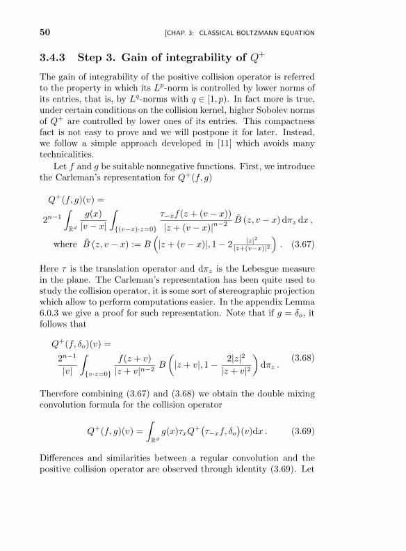
3.4.3 Step 3. Gain of integrability of Q+

The gain of integrability of the positive collision operator is referredto the property in which its Lp-norm is controlled by lower norms ofits entries, that is, by Lq-norms with q ∈ [1, p). In fact more is true,under certain conditions on the collision kernel, higher Sobolev normsof Q+ are controlled by lower ones of its entries. This compactnessfact is not easy to prove and we will postpone it for later. Instead,we follow a simple approach developed in [11] which avoids manytechnicalities.

Let f and g be suitable nonnegative functions. First, we introducethe Carleman’s representation for Q+(f, g)

Q+(f, g)(v) =

2n−1∫Rd

g(x)

|v − x|

∫{(v−x)·z=0}

τ−xf(z + (v − x))

|z + (v − x)|n−2B (z, v − x) dπz dx ,

where B (z, v − x) := B(|z + (v − x)|, 1− 2 |z|2

|z+(v−x)|2

). (3.67)

Here τ is the translation operator and dπz is the Lebesgue measurein the plane. The Carleman’s representation has been quite used tostudy the collision operator, it is some sort of stereographic projectionwhich allow to perform computations easier. In the appendix Lemma6.0.3 we give a proof for such representation. Note that if g = δo, itfollows that

Q+(f, δo)(v) =

2n−1

|v|

∫{v·z=0}

f(z + v)

|z + v|n−2B

(|z + v|, 1− 2|z|2

|z + v|2

)dπz .

(3.68)

Therefore combining (3.67) and (3.68) we obtain the double mixingconvolution formula for the collision operator

Q+(f, g)(v) =

∫Rdg(x)τxQ

+(τ−xf, δo

)(v)dx . (3.69)

Differences and similarities between a regular convolution and thepositive collision operator are observed through identity (3.69). Let

ii


ii

ii


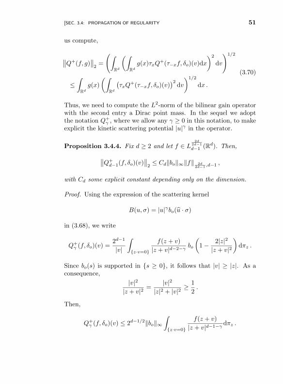
us compute,

∥∥Q+(f, g)∥∥2

=

(∫Rd

(∫Rdg(x)τxQ

+(τ−xf, δo)(v)dx

)2

dv

)1/2

≤∫Rdg(x)

(∫Rd

(τxQ

+(τ−xf, δo)(v))2

dv

)1/2

dx .

(3.70)

Thus, we need to compute the L2-norm of the bilinear gain operatorwith the second entry a Dirac point mass. In the sequel we adoptthe notation Q+

γ , where we allow any γ ≥ 0 in this notation, to makeexplicit the kinetic scattering potential |u|γ in the operator.

Proposition 3.4.4. Fix d ≥ 2 and let f ∈ L2d

2d−1

d−1 (Rd). Then,∥∥Q+d−1(f, δo)(v)

∥∥2≤ Cd‖bo‖∞‖f‖ 2d

2d−1 ,d−1,

with Cd some explicit constant depending only on the dimension.

Proof. Using the expression of the scattering kernel

B(u, σ) = |u|γbo(u · σ)

in (3.68), we write

Q+γ (f, δo)(v) =

2d−1

|v|

∫{z·v=0}

f(z + v)

|z + v|d−2−γbo

(1− 2|z|2

|z + v|2

)dπz .

Since bo(s) is supported in {s ≥ 0}, it follows that |v| ≥ |z|. As aconsequence,

|v|2

|z + v|2=

|v|2

|z|2 + |v|2≥ 1

2.

Then,

Q+γ (f, δo)(v) ≤ 2d−1/2‖bo‖∞

∫{z·v=0}

f(z + v)

|z + v|d−1−γdπz .

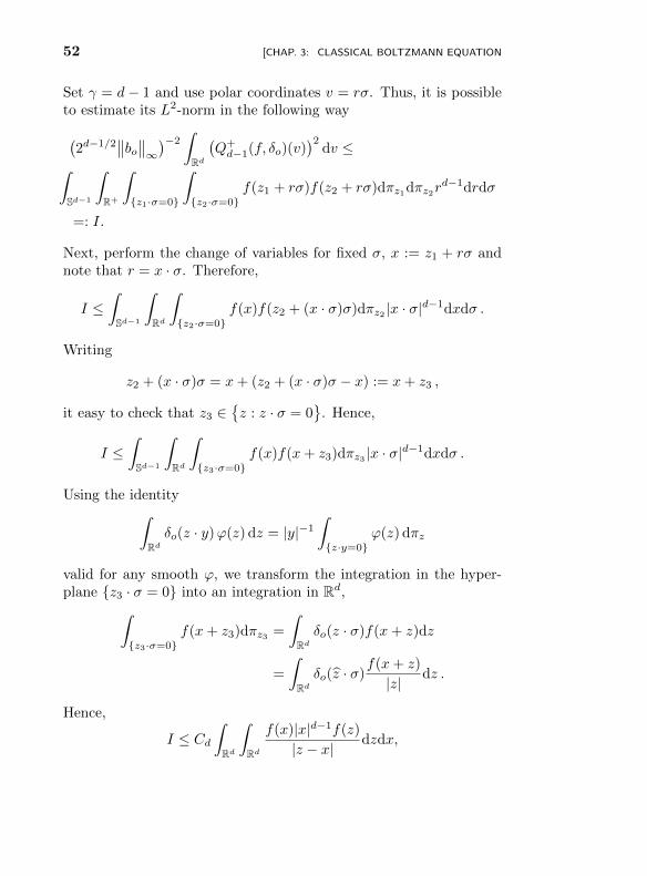
ii


ii

ii


Set γ = d− 1 and use polar coordinates v = rσ. Thus, it is possibleto estimate its L2-norm in the following way(

2d−1/2∥∥bo∥∥∞)−2 ∫

Rd

(Q+d−1(f, δo)(v)

)2dv ≤∫

Sd−1

∫R+

∫{z1·σ=0}

∫{z2·σ=0}

f(z1 + rσ)f(z2 + rσ)dπz1dπz2rd−1drdσ

=: I.

Next, perform the change of variables for fixed σ, x := z1 + rσ andnote that r = x · σ. Therefore,

I ≤∫Sd−1

∫Rd

∫{z2·σ=0}

f(x)f(z2 + (x · σ)σ)dπz2 |x · σ|d−1dxdσ .

Writing

z2 + (x · σ)σ = x+ (z2 + (x · σ)σ − x) := x+ z3 ,

it easy to check that z3 ∈{z : z · σ = 0

}. Hence,

I ≤∫Sd−1

∫Rd

∫{z3·σ=0}

f(x)f(x+ z3)dπz3 |x · σ|d−1dxdσ .

Using the identity∫Rdδo(z · y)ϕ(z) dz = |y|−1

∫{z·y=0}

ϕ(z) dπz

valid for any smooth ϕ, we transform the integration in the hyper-plane {z3 · σ = 0} into an integration in Rd,∫

{z3·σ=0}f(x+ z3)dπz3 =

∫Rdδo(z · σ)f(x+ z)dz

=

∫Rdδo(z · σ)

f(x+ z)

|z|dz .

Hence,

I ≤ Cd∫Rd

∫Rd

f(x)|x|d−1f(z)

|z − x|dzdx,

ii


ii

ii


where the constant can be taken as

Cd =

∫Sd−1

δo(z · σ)dσ =∣∣Sd−2∣∣ ∫ 1

−1δo(s)(1− s2)

d−32 ds =

∣∣Sd−2∣∣ .Finally, recalling the Hardy-Littlewood-Sobolev inequality we havefor any r ∈ (1,∞),

I ≤ Cd∥∥f | · |d−1∥∥

r′

∥∥f ∗ | · |−1∥∥r≤ Cd,r

∥∥f | · |d−1∥∥r′‖f‖p,

where 1/p+ 1/d = 1 + 1/r. Choosing p = r′, that is p = 2d2d−1 , yields

I ≤ Cd,r∥∥f | · |d−1∥∥ 2d

2d−1

∥∥f∥∥ 2d2d−1

≤ Cd,r ‖f‖2 2d2d−1 ,d−1

.

Since r := r(d) the result follows.

Let us come back to the estimation of the L2-norm of Q+. Fixa dimension d ≥ 2 and recall that the physical accepted values of γsatisfy 0 < γ ≤ 1 ≤ d− 1. Thus,

|u|γ ≤ εs′

s′+

1

sεs|u|γs s = d−1

γ , ε > 0 . (3.71)

Additionally, we write the scattering kernel bo = b1o + b∞o with

(1) b1o ≥ 0 having small mass, say ‖b1o‖L1(Sd−1) = δ > 0.

(2) And, b∞o ≥ 0 essentially bounded and such that b∞o ≤ b1o. Ofcourse, ‖b∞o ‖∞ will depend in general on δ.

Therefore, for any k ≥ −γ it follows that∥∥Q+γ (f, g)

∥∥2,k

=∥∥Q+

γ,b1o(f, g) +Q+

γ,b∞o(f, g)

∥∥2,k

≤∥∥Q+

γ,b1o(f, g)

∥∥2,k

+∥∥Q+

γ,b∞o(f, g)

∥∥2,k

≤∥∥Q+

γ,b1o(f, g)

∥∥2,k

+ εs′

s′

∥∥Q+o,b∞o

(f, g)∥∥2,k

+ 1sεs

∥∥Q+d−1,b∞o

(f, g)∥∥2,k.

(3.72)

ii


ii

ii


For the last inequality we have used (3.71). Using Proposition 3.4.2it follows that∥∥Q+

γ,b1o(f, g)

∥∥2,k≤ 2

d+γ2 ‖b1o‖

1/21 ‖f‖2,k+γ‖g‖1,k+2γ

= 2d+γ2

√δ ‖f‖2,k+γ‖g‖1,k+2γ ,∥∥Q+

o,b∞o(f, g)

∥∥2,k≤ 2

d+γ2 ‖b∞o ‖

1/21 ‖f‖2,k+‖g‖1,k+

≤ 2d+γ2 ‖f‖2,k+‖g‖1,k+ ,

where, in the last inequality, we introduced k+ := max{0, k}. For thelatter term in (3.72) use (3.70) and Proposition 3.4.4. Thus, whenk = 0∥∥Q+

d−1,b∞o(f, g)

∥∥2≤∫Rd

∥∥τxQ+d−1,b∞o

(τ−xf, δo)∥∥2g(x)dx

≤ Cd‖b∞o ‖∞∫Rd

∥∥τ−xf∥∥ 2d2d−1 ,d−1

g(x)dx

≤ Cd,δ‖f‖ 2d2d−1 ,d−1

‖g‖1,d−1 .

Therefore, when a weight k ≥ −γ is used∥∥Q+d−1,b∞o

(f, g)∥∥2,k≤∥∥Q+

d−1,b∞o(f〈·〉k

+

, g〈·〉k+

)∥∥2

≤ Cd,δ‖f‖ 2d2d−1 ,k

++d−1‖g‖1,k++d−1 .

This proves the following proposition.

Proposition 3.4.5. Fix d ≥ 2 and γ ∈ (0, 1]. The collision operatorsatisfies the estimate for any ε > 0, δ > 0 and k ≥ −γ

‖Q+γ (f, g)‖2,k ≤ 2

d+γ2

√δ ‖f‖2,k+γ‖g‖1,k+2γ +

2d+γ2εs′

s′‖f‖2,k+‖g‖1,k+ +

Cd,δsεs‖f‖ 2d

2d−1 ,k++d−1‖g‖1,k++d−1 ,

where s = d−1γ , k+ = max{0, k}, and Cd,δ depends only on d and

δ. In the case s = 1, the second term in the right side vanishes andε = 1.

We have all the ingredients to prove the main result of this sec-tion, propagation of L2 integrability for the Boltzmann homogeneousequations.

ii


ii

ii


Theorem 3.4.6. Fix a dimension d ≥ 2 and potential γ ∈ (0, 1].Assume Grad’s cutoff in the angular kernel (normalized to one). Ad-ditionally, fix k ≥ 0 and assume an initial estate fo ∈ L1

ko∩L2k. Then,

the solution f to the homogeneous Boltzmann equation propagates L2k

integrabilitysupt≥0

∥∥f(t)∥∥2,k≤ C(fo) .

The constant depends on the mass, mko(fo) and ‖fo‖2,k, where

ko = max{k + 3γ

2 , k + γ + dd−1(d− 1− γ

)}.

Proof. Fix k ≥ 0 and multiply the Boltzmann equation (3.50) byf〈·〉k and integrate in velocity. This process leads to

d

dt‖f(t)‖2

2, k2=

∫RdQ+(f, f)(v)f(v)〈v〉kdv

−∫RdQ−(f, f)(v)f(v)〈v〉kdv .

(3.73)

Using Lemma 3.4.3 one obtains∫RdQ−(f, f)(v)f(v)〈v〉kdv

=

∫Rdf(v)2〈v〉k

(f ∗ | · |γ

)(v)dv ≥ C(fo)

∥∥f∥∥22, k+γ2

.

(3.74)

For the first term in (3.73) use Proposition 3.4.5, with f = g, toconclude∫

Rd

(Q+(f, f)(v)〈v〉

k−γ2

)f(v)〈v〉

k+γ2 dv ≤

2d+γ2

(√δ ‖f‖2, k+γ2 ‖f‖1, k+3γ

2+εs′

s′‖f‖

2,(k−γ2

)+‖f‖1,(k−γ2

)++Cd,δsεs‖f‖

2d2d−1 ,

(k−γ2

)++d−1

‖f‖1,(k−γ2

)++d−1

)∥∥f∥∥2, k+γ2

.

(3.75)

Since 2d2d−1 < 2, it is possible to use Lebesgue’s interpolation

‖f‖2d

2d−1 ,(k−γ2

)++d−1

≤ ‖f‖1d

2, k+γ2‖f‖

d−1d

1, k2+γ+dd−1 (d−1−γ)

. (3.76)

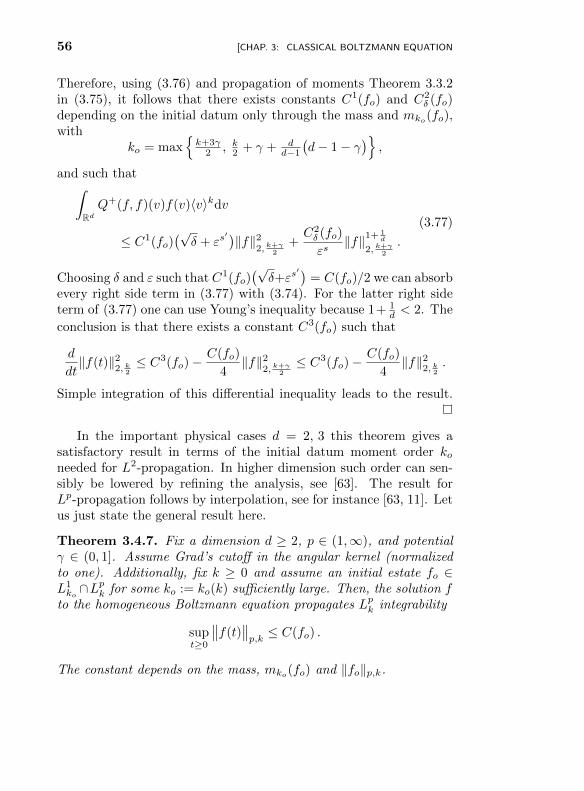
ii


ii

ii


Therefore, using (3.76) and propagation of moments Theorem 3.3.2in (3.75), it follows that there exists constants C1(fo) and C2

δ (fo)depending on the initial datum only through the mass and mko(fo),with

ko = max{k+3γ

2 , k2 + γ + dd−1(d− 1− γ

)},

and such that∫RdQ+(f, f)(v)f(v)〈v〉kdv

≤ C1(fo)(√δ + εs

′)‖f‖2

2, k+γ2+C2δ (fo)

εs‖f‖1+

1d

2, k+γ2.

(3.77)

Choosing δ and ε such that C1(fo)(√δ+εs

′)= C(fo)/2 we can absorb

every right side term in (3.77) with (3.74). For the latter right sideterm of (3.77) one can use Young’s inequality because 1+ 1

d < 2. The

conclusion is that there exists a constant C3(fo) such that

d

dt‖f(t)‖2

2, k2≤ C3(fo)−

C(fo)

4‖f‖2

2, k+γ2≤ C3(fo)−

C(fo)

4‖f‖2

2, k2.

Simple integration of this differential inequality leads to the result.

In the important physical cases d = 2, 3 this theorem gives asatisfactory result in terms of the initial datum moment order koneeded for L2-propagation. In higher dimension such order can sen-sibly be lowered by refining the analysis, see [63]. The result forLp-propagation follows by interpolation, see for instance [63, 11]. Letus just state the general result here.

Theorem 3.4.7. Fix a dimension d ≥ 2, p ∈ (1,∞), and potentialγ ∈ (0, 1]. Assume Grad’s cutoff in the angular kernel (normalizedto one). Additionally, fix k ≥ 0 and assume an initial estate fo ∈L1ko ∩L

pk for some ko := ko(k) sufficiently large. Then, the solution f

to the homogeneous Boltzmann equation propagates Lpk integrability

supt≥0

∥∥f(t)∥∥p,k≤ C(fo) .

The constant depends on the mass, mko(fo) and ‖fo‖p,k.

ii


ii

ii


3.4.4 Step 4. Propagation of Sobolev regularity

Before entering in details about propagation of regularity for the ho-mogeneous Boltzmann equation, we will need a result very much re-lated to Proposition 3.4.4, yet, of slightly different nature. It is aboutthe fact that under certain integrability condition on the angular ker-nel, higher Sobolev norms can be controlled by lower ones. There areseveral versions of this fact, see for instance [54, 55, 75, 63]. For ourpurpose, it will suffice to follow a neat result that was brought in [24].

Proposition 3.4.8. Let bo ∈ L2(Sd−1). Then∥∥Q+γ (f, g)

∥∥Hd−12 (Rd)

≤ Cd‖bo‖2 ‖f‖2,γ+1‖g‖2,γ+1 , γ ≥ 0 .

Proof. The proof is based on the Fourier transform of the gain oper-ator Q+ using the weak formulation

F{Q+(f, g)

}(ξ) =

∫RdQ+(f, g)(v)e−iv·ξdv

=

∫R2d

f(v)g(v∗)|u|γ(∫

Sd−1

e−iv′·ξbo(u · σ)dσ

)dv∗dv .

For the average in the sphere, it follows that∫Sd−1

e−iv′·ξb(u · σ)dσ = e−i(v−

u2 )·ξ

∫Sd−1

e−i|u||ξ|

2 ξ·σbo(u · σ)dσ

= e−i(v−u2 )·ξ

∫Sd−1

e−i|u||ξ|

2 u·σbo(ξ · σ)dσ .

The last equality results after interchanging u ↔ ξ which is allowedsince the integral on the sphere is a function of the inner product u · ξonly (and the norms |u| and |ξ|). Thus,

F{Q+(f, g)

}(ξ) =∫

Sd−1

(∫R2d

f(v)g(v∗)|u|γe−i(ξ+|ξ|σ

2 )·ve−i(ξ−|ξ|σ

2 )·v∗dv∗dv)bo(ξ · σ)dσ

=

∫Sd−1

F{F}( ξ+|ξ|σ

2 , ξ−|ξ|σ2

)bo(ξ · σ)dσ . (3.78)

ii


ii

ii


where F (v, v∗) := f(v)g(v∗)|u|γ . The use of the Fourier transform inthe Boltzmann equation was proposed in [17] for Maxwell moleculesand later refined to other potentials. Thus, using Cauchy-Schwarz’sinequality∣∣F{Q+(f, g)

}(ξ)∣∣2 ≤ ‖bo‖22 ∫

Sd−1

∣∣∣F{F}( ξ+|ξ|σ2 , ξ−|ξ|σ2

)∣∣∣2dσ .

(3.79)Now, compute∫

Sd−1

∣∣∣F{F}( ξ+|ξ|σ2 , ξ−|ξ|σ2

)∣∣∣2dσ

=

∫Sd−1

∫ ∞|ξ|−∂r

∣∣∣F{f(v)g(v∗)|u|γ}(

ξ+rσ2 , ξ−rσ2

)∣∣∣2drdσ

=

∫Sd−1

∫ ∞|ξ|F{F}(∇2F

{F}−∇1F

{F})(

ξ+rσ2 , ξ−rσ2

)· σdrdσ

=

∫{|η|≥|ξ|}

F{F}F{− i(v∗ − v)F

}(ξ+η2 , ξ−η2

)· η dη

|η|d−1.

(3.80)

As a consequence from (3.79) and (3.80)

‖bo‖−22

∥∥Q+(f, g)∥∥2Hd−12

=

∫Rd

∣∣∣F{Q+(f, g)}

(ξ)|ξ|d−12

∣∣∣2dξ

≤∫R2d

∣∣∣F{F}F{− i(v∗ − v)F}(

ξ+η2 , ξ−η2

)∣∣∣dηdξ

= 2d∥∥F{F}F{(v∗ − v)F}

∥∥L1(R2d)

≤ 2d∥∥F{F}∥∥

L2(R2d)

∥∥F{(v∗ − v)F}‖L2(R2d) .

Fourier isometry give us

∥∥F{F}∥∥L2(R2d)

= (2π)2d∥∥F∥∥

L2(R2d)≤ (2π)2d

∥∥f∥∥2,γ‖g∥∥2,γ

,∥∥F{(v∗ − v)F}∥∥L2(R2d)

= (2π)2d∥∥(v∗ − v)F

∥∥L2(R2d)

≤ (2π)2d∥∥f∥∥

2,γ+1‖g∥∥2,γ+1

.

ii


ii

ii


Now, the way one uses Proposition 3.4.8 to prove propagationof Sobolev regularity is the following. Set the dimension d = 3 forsimplicity and consider an initial datum fo ∈ L1

k(γ) ∩ L21+γ , with

k(γ) sufficiently large, belonging to H1(Rd). Then, differentiatingthe Boltzmann equation by vi

∂tfi = ∂viQ+(f, f)− fi

(f ∗ | · |γ

)− f

(f ∗ ∂vi | · |γ

). (3.81)

Here of course fi := ∂vif . Recall the lower bound on the Q− givenin Lemma 3.4.3, and also note the simple estimate

f ∗ ∂vi | · |γ ≤ cγ(‖f‖2 +m(fo)

)≤ C(fo) , γ ∈ (0, 1] .

The last inequality follows from Theorem 3.4.6 since fo ∈ L2(Rd).As a consequence, multiplying equation (3.81) by fi and integratingin velocity one concludes

12

d

dt‖fi‖22 ≤ ‖∂viQ+(f, f) fi‖1 + C(fo)‖fi f‖1 − c(fo)‖fi‖22,γ/2 .

(3.82)Using Proposition 3.4.8 it follows that (here d−1

2 = 1)

‖∂viQ+(f, f) fi‖1 ≤ ‖∂viQ+(f, f)‖2‖fi‖2≤ Cd‖bo‖2‖f‖22,γ+1‖fi‖2 ≤ C(fo)‖fi‖2 .

(3.83)

In summary, gathering (3.82) and (3.83)

12

d

dt‖fi‖22 ≤ C(fo)‖fi‖2 − c(fo)‖fi‖22,γ/2 . (3.84)

This a priori estimate readily implies that

supt≥0‖f‖H1 ≤ C(fo) . (3.85)

The dependence of the constant is written in terms of the L1k(γ)∩L

21+γ

norms and the H1-regularity of the initial data. Higher Sobolev regu-larity is implemented with induction using the differentiation Leibnizrule holding for the collision operator

∂νvQ(f, g) =

ν∑η=0

(νη

)Q(∂ηvf, ∂

ν−ηv g

),

ii


ii

ii


where ν and η are multi-indexes. The details are left to the readeror can be found in [63].

Theorem 3.4.9. Let γ ∈ (0, 1] and bo ∈ L2(Sd−1). Assume fo ∈L12 ∩ Hk

k(1+γ). Then, the solution of the homogeneous Boltzmannequation satisfies

supt≥0‖f‖Hk ≤ Ck(fo) , k ∈ N.

3.5 Entropy dissipation method and timeasymptotic

The starting point of this section is an essential process in physics: theOrnstein–Uhlenbeck process. Such process is describing the velocityof a particle that experiences friction and Brownian forces (thermal-ization)

dv(t) = −ν v(t)dt+ η dB(t) , v(0) = vo . (3.86)

Here the non negative parameters ν and η are the friction and ther-malization coefficients respectively. The Brownian motion is addedto the equation to model the influence of a smaller scale physicsinfluencing the particle, such as, small molecules in continuous col-lision with this macroscopic particle. As a consequence, the frictionterm decreases the kinetic energy of the particle while the thermal-ization increases it. The Ornstein–Uhlenbeck stochastic equation hasKolmogorov forward equation (commonly known as Fokker–Planckequation)

∂tf = ν∇v · (vf) +η2

2∆vf , f(0) = fo . (3.87)

Equation (3.87) does not conserves momentum or energy, due to colli-sions with the micro-scale, only conserves mass. However, it is easy tosee that energy will remain uniformly bounded. Furthermore, giventhe physics of the problem one expects a non trivial relaxation of thisprocess as time evolve. Let us prove this by introducing the relativeentropy (compare with 3.7)

H(f∣∣M) =

∫Rdf(v) log

f(v)

M(v)dv , M(v) =

e−|v|22

(2π)d2

. (3.88)

ii


ii

ii

[SEC. 3.5: ENTROPY DISSIPATION METHOD AND TIME ASYMPTOTIC 61

Thus, set ν = 1 and η =√

2 for simplicity and multiply the Fokker–

Planck equation (3.87) by log( f(v)M(v)

), one finds2

d

dtH(f∣∣M) = −I

(f∣∣M) , (3.89)

where I is the relative Fisher information

I(f∣∣M) :=

∫Rdf(v)

∣∣∣∇v logf(v)

M(v)

∣∣∣2dv . (3.90)

Using the Stam–Gross logarithmic Sobolev inequality, see [69]

H(f∣∣M) ≤ 1

2I(f∣∣M) , (3.91)

valid for any f ∈ L1(Rd) having unit mass since M is a normalizedGaussian. Therefore, using (3.91) in (3.89) one gets

H(f∣∣M) ≤ e−2tH(fo∣∣M) .

With this at hand it is possible to invoke Csiszar–Kullback–Pinskerinequality

‖f −M‖1 ≤√

2H(f∣∣M) ,

to deduce that the distribution of the Ornstein–Uhlenbeck processexperiments an exponential relaxation in the L1-metric, provided theinitial datum fo has finite second moment (energy) and entropy, to-wards a Gaussian distribution. We refer to [71] for an ample discus-sion on the topic and references. Let us conclude this short discussionby noticing that multiplying equation (3.87) by log(f), it is concludedafter integration by parts that

d

dtH(f) = −I(f) + d = −I(f) + I(M) .

Here I is the Fisher information (given by (3.90) with M ≡ 1). Now,integrate in the time interval [0,∞), use that f(t) → M in L1 and

2Simply observe that v = −∇M(v)

M(v).

ii


ii

ii


the fact that f has second moment uniformly bounded, to concludethat

H(fo)−H(M) =

∫ ∞0

(I(f(s))− I(M)

)ds . (3.92)

Representation formula (3.92) will be important in the next subsec-tion and it is valid for any function fo ∈ L1(Rd) with unitary massand finite energy.

3.5.1 Relaxation of the linear Boltzmann model

The Ornstein–Uhlenbeck process, as important as it is, does notpresent big analytic challenges. In fact, the machinery just intro-duced previously it is not needed to prove relaxation to a Gaussianstate. The reason is that one can easily compute the Green functionof the Fokker-Planck equation (3.87): Assume a initial particle dis-tribution fo(v) = δo(v −w), then, the probability distribution of theOrnstein–Uhlenbeck process evolves as

ht(v, w) =e− 1

2|v−e−tw|2

1−e−2t(2π(1− e−2t)

) d2

.

Thus, the semigroup St of the Fokker-Planck equation has the explicitform

Stf(v) =

∫Rdht(v, w) f(w)dw = edt

(Ht ∗ Ft

)(v) ,

where Ht(v) :=e− 1

2|v|2

1−e−2t(2π(1− e−2t)

) d2

, Ft(v) := f(et v) .

(3.93)

From here it is clear that Stf → M as t → ∞ at exponentialrate. This observation, however, does not mean that the Ornstein–Uhlenbeck process is just a simple example to introduce advancedtools, we will see next that it plays a central role in more compli-cated processes having distributions evolving to Gaussians.

Let us try to apply the entropy relaxation method to the linearBoltzmann model with Maxwell molecules interactions, that is, whenthe collision operator has potential γ = 0. This problem is quite

ii


ii

ii


interesting because the Boltzmann model represents a jump processin contrast with the Fokker–Planck equation. The linear Boltzmannequation reads

∂tf = Qo(f,M) =: L(f) , f(0) = fo . (3.94)

The physics representing this equation is a cloud of particles collid-ing with an homogeneous background (of particles) having a Gaus-sian distribution. This model approximates a regime where the back-ground particles are many in comparison with the particles distributedwith f . In such a case, particle–particle interaction is a secondaryphenomena compared to the particle–background interaction. Thus,thermodynamics tells us that it should be the case that f → M astime evolves. A first indication that this is in fact the case comesfrom the equations for the momentum and energy of f

dv(f)

dt= − 1−λ

2 v(f) , v(f)(t) :=

∫Rdf(t, v) v dv ,

dm2(f)

dt= − 1−λ

2

(m2(f)−m2(M)

),

(3.95)

where the parameter λ is given by

λ :=

∫Sd−1

(u · σ) bo(u · σ)dσ ∈ (0, 1) . (3.96)

Equations (3.95) follows after multiplying (3.94) with v and |v|2 andintegrating in velocity. Thus, v(f) → v(M) and m2(t) → m2(M)at exponential rate 1−λ

2 . We observe that closed equations for mo-ments is a benefit only happening for Maxwellian interactions due tohomogeneity of the potential.

The problem of exponential converge of the equation (3.94) to-wards the Gaussian background has been nicely treated in [16] forMaxwell molecules and other potentials as well. We follow here theirpresentation and argument only in the case of Maxwell molecules andrefer to [16] for a complete discussion to more general potentials andlinks to logarithmic Sobolev inequalities. The idea is, as presentedpreviously, to control the relative entropy with the entropy dissipa-tion which is the analogous of the Fisher information in the case of

ii


ii

ii


Boltzmann

d

dtH(f(t)

∣∣M) =

∫RdL(f(t))(v) log

f(t, v)

M(v)dv = −D

(f(t)

), (3.97)

where

D(f) := 12

∫R2d

M(v)M(v∗)×(∫Sd−1

Φ( f(v)

M(v),f(v′)

M(v′)

)bo(u · σ)dσ

)dv∗dv ,

(3.98)

and Φ(x, y) := (x− y) log(x/y) ≥ 0.

Theorem 3.5.1. The functional inequality

D(f) ≥ 1−λ2 H

(f∣∣M)

holds for any probability distribution f ∈ L1(Rd). The constant λ isgiven in (3.96).

There are several interesting steps in proving Theorem 3.5.1, eachof them important in their own right. The first step consists in thefollowing commutativity property: Let St be the semigroup generatedby the Fokker-Planck equation (3.93), then

Q+(Stf,Stg) = StQ+(f, g) , t ≥ 0 , (3.99)

valid for any f ∈ L1(Rd) with finite energy. This commutativityproperty looks odd, as one would expect such property holding forthe generator of the Ornstein–Uhlenbeck process (the adjoint of St)related to the Kolmogorov backward equation rather than for St (re-lated to the Kolmogorov forward equation). Indeed, propagatingtwo particles backward in time using the Ornstein–Uhlenbeck processand, then, perform a collision looks the same as collide the particlesand, then, propagate backwards in time. However, one recalls thatfor elastic interactions the collision law is time symmetric, pre/poscollision laws are interchangeable, which explains, at least intuitively,identity (3.99). The proof of (3.99) goes by direct computation using

ii


ii

ii


Fourier transform in velocity. Indeed, recalling formula (3.78)

F{Q+(Ht ∗ Ft, Ht ∗Gt

)}(ξ)

=

∫Sd−1

F{Ht ∗ Ft

}(ξ+)F

{Ht ∗Gt

}(ξ−) bo(ξ · σ)dσ

=

∫Sd−1

F{Ht}(ξ+)F

{Ht}(ξ−)F

{Ft}

(ξ+)F{Gt}

(ξ−) bo(ξ · σ)dσ .

Here ξ± = 12 (ξ ± |ξ|σ). Now, Ht is a normalized Gaussian, so its

Fourier transform is a unitary Gaussian. In addition, note that |ξ|2 =|ξ+|2 + |ξ−|2, therefore

F{Ht}(ξ+)F

{Ht}(ξ−) = F

{Ht}(ξ) .

As a consequence,

F{Q+(Ht ∗ Ft, Ht ∗Gt

)}(ξ) = F

{Ht}F

{Q+(Ft, Gt

)}(ξ) .

And thus,

Q+(Stf,Stg) = Ht ∗Q+(Ft, Gt

)= edt

(Ht ∗Q+

(f, g)t

)= StQ+

(f, g).

The second step is further proof of the importance of the Ornstein–Uhlenbeck process, the complete proof can be found in [57].

Proposition 3.5.2. Let I be the Fisher information and Q+ be theBoltzmann collision operator with Maxwellian interactions. Then,

I(Q+(f, g)

)≤ 1+λ

2 I(f) + 1−λ2 I(g) ,

valid for any sufficiently smooth probability densities f, g. The con-stant λ is given in (3.96).

Corollary 3.5.3. Let Q+ be the Boltzmann collision operator withMaxwellian interactions. Then,

H(Q+(f, g)

)≤ 1+λ

2 H(f) + 1−λ2 H(g)

for any probability densities f, g.

ii


ii

ii


Proof. Note that identity (3.92) can be written in terms of the Fokker-Planck semigroup St

H(f)−H(M) =

∫ ∞0

(I(Stf)− I(M)

)dt

for any probability density f ∈ L1(Rd) with finite energy. Thus,taking f ≡ Q+(f, g) it follows that

H(Q+(f, g))−H(M) =

∫ ∞0

(I(StQ+(f, g))− I(M)

)dt

=

∫ ∞0

(I(Q+(Stf,Stg))− I(M)

)dt

≤ 1+λ2

∫ ∞0

(I(Stf)− I(M)

)dt+ 1−λ

2

∫ ∞0

(I(Stg)− I(M)

)dt

= 1+λ2 H(f) + 1−λ

2 H(g)−H(M) .

where we used the commutativity property (3.99) and Proposition3.5.2.

Corollary 3.5.4. Let L be the linear Boltzmann collision operatorwith Maxwellian interactions. Then,

H(L+(f)

∣∣M) ≤ 1+λ2 H

(f∣∣M)

for any probability density f . Here, of course, L(f) =: L+(f)− f .

Proof. Let us use Corollary 3.5.3 with g ≡M to estimate

H(L+(f)

∣∣M) = H(L+(f)

)−∫RdL+f logMdv

≤ 1+λ2 H

(f)

+ 1−λ2 H

(M)−∫RdL+f logMdv

= 1+λ2 H

(f∣∣M)+ 1−λ

2

∫Rd

(M − f

)logMdv −

∫RdL(f) logMdv

= 1+λ2 H

(f∣∣M) .

We used conservation of mass and the equation for the energy givenin (3.95) to conclude that the last two terms cancel out.

ii


ii

ii


Proof of Theorem 3.5.1

Estimate the dissipation of entropy as follows

D(f) = −∫RdL(f) log

f

Mdv

= H(f∣∣M)−H

(L+(f)

∣∣M)+H(L+(f)

∣∣f)≥ H

(f∣∣M)−H

(L+(f)

∣∣M) ≥ 1−λ2 H

(f∣∣M) .

In the first inequality we used thatH(L+(f)

∣∣f) ≥ 0 because the massof f and L+f are both one. The second inequality follows from Corol-lary 3.5.4. �

As a consequence of Theorem 3.5.1, the solution of (3.94) satisfiesthe exponential relaxation

H(f∣∣M) ≤ H(fo∣∣M)e− 1−λ

2 t ,

which seems to be the sharp rate of relaxation (by comparing with therelaxation rate of the momentum and energy). Furthermore, Csiszar–Kullback–Pinsker inequality implies the relaxation in the L1-metric

‖f −M‖1 ≤√

2H(f∣∣M) ≤√2H

(fo∣∣M)e− 1−λ

4 t .

Let us finishing this discussion by mentioning that the nonlinearBoltzmann equation relaxation has already been studied with en-tropy methods, we refer to [67, 71] and their related references, bysolving the so-called Cercignani’s conjecture. Needless to say, in thenonlinear cases an entropy functional becomes more valuable sinceit is unique to the process in question as opposed to the linear casewhere there may be plenty of entropy functionals. Interestingly, theprogram presented here for the linear case follows essentially the samesteps of the program given in [67] for the nonlinear case (up to math-ematical technicalities).

ii


ii

ii


3.6 More on the Cauchy theory for Boltz-mann

There is a vast literature for the Cauchy problem treating kineticequations. In particular, the theory of existence and uniqueness ofsolutions for the Boltzmann equation in a Gaussian–perturbativeregime has been pursued quite successfully by an number of au-thors. The methods include linearization of the collision operatorand the development of a mathematical machinery used to controlthe non linear dynamic of the model using the linear dynamics.These ideas are far reaching and have many applications, we referto [32, 33, 44, 45, 46] for an initiation on this theory.

ii


ii

ii

Chapter 4

Dissipative Boltzmannequation

4.1 Cucker-Smale model and self organi-zation

We start this discussion on dissipative systems with an example thatwe discussed at the beginning of this note (Section 1), the Cucker-Smale (CS) model. We recall that the CS model represents a systemof N particles interacting by an average law of friction through afriction potential

dxidt

= vi ,dvidt

=1

N

∑j 6=i

Uf(|xj − xi|

)(vj − vi) , (4.1)

where (xi, vi) represents the position and velocity of the i-particle.In the applied literature, the CS model has been used to explain“flocking” of birds, school of fish, swarming of bacteria and otherbiological organisms. The word flocking represents a phenomenonin which self-propelled individuals organize into an ordered motion.In the following lines we present a simple analysis on the particlesystem (4.1) and its kinetic equation to represent, up to some extent,mathematically this phenomenon. The main assumption simply read:

69

ii


ii

ii

70 [CHAP. 4: DISSIPATIVE BOLTZMANN EQUATION

Uf is Lipschitz continuous, decreasing and such that

c

(1 + |x|2)β≤ Uf (|x|) ≤ C , β ≥ 0 . (4.2)

The position and velocity of the center of mass of the particles isgiven by

xc(t) :=1

N

N∑i=1

xi(t) , vc(t) :=1

N

N∑i=1

vi(t) . (4.3)

Summing over all velocities in the equation for the velocity in (4.1)and using the symmetry of the interaction it follows that

vc(t) = vc(0) , xc(t) = xc(0) + t vc(0) . (4.4)

That is, the system conserves momentum, and hence, the trajectoryof the center of mass is just a straight line. Define the fluctuationsof the particles around the center of mass as xi(t) := xi(t) − xc(t)and vi(t) := vi(t) − vc(t) and introduce the variance, or fluctuation,functions

X(t) :=

N∑i=1

|xi(t)|2 , V (t) :=

N∑i=1

|vi(t)|2 . (4.5)

Then, we can show the formation of a flock by showing that V (t)decays towards zero and X(t) remains uniformly bounded. In otherwords, in the long run particles will travel in one group and sharingthe same velocity. Moreover, if the decay on V (t) is sufficiently fast,this behavior will be stable under external perturbations, refer to [49]for ample discussion. First, let us investigate the spatial fluctuationwith the following computation

dX

dt=

2

N

N∑i=1

(xi − xc

)·(dxidt− dxc

dt

)=

2

N

N∑i=1

(xi − xc

)·(vi − vc

)≤ 2√X√V ,

(4.6)

ii


ii

ii

[SEC. 4.1: CUCKER-SMALE MODEL AND SELF ORGANIZATION 71

where the last estimate follows from Cauchy-Schwarz inequality. Sec-ond, let us estimate the velocity fluctuation in the following way

dV

dt= − 1

N2

∑1≤i,j≤N

Uf (|xj − xi|)|vj − vi|2

≤ −Uf(2√X)

N2

∑1≤i,j≤N

|vj − vi|2

= −2Uf(2√X)( 1

N

N∑i=1

|vi|2 − v2c)

= −2Uf(2√X)V ≤ 0 .

(4.7)

For the inequality we have used that Uf (|xj − xi|) ≥ Uf(2√X), for

any i, j, since Uf (·) is decreasing. Thus, thanks to (4.7) and (4.6) itfollows that

V (t) ≤ Vo ,√X(t) ≤

√Xo +

√Vo t . (4.8)

Theorem 4.1.1. (Flock formation) Let (xi, vi) be solutions to the CSmodel (4.1) with Uf satisfying (4.2). Then, the fluctuation functionssatisfy √

X(t) ≤√Xo + C , V (t) ≤ Vo e−c1t , β ∈ [0, 12 ] .

The constants C and c1 are positive, finite and explicit in terms of theinitial fluctuation (Xo, Vo), the model parameter β and the constantc defining the lower bound for Uf .

Proof. Integrating inequality (4.7) gives

V (t) ≤ Vo e−2∫ t0Uf

(2√X(s)

)ds . (4.9)

Assume first that β ∈ [0, 1/2). Thus, using estimate (4.8) on thespatial fluctuation and assumption (4.1), it is not very difficult toestimate the time integral

2

∫ t

0

Uf(2√X(s)

)ds ≥ c

(1− 2β)V βot1−2β .

ii


ii

ii


Plugging this estimate in (4.9), one upgrades the estimate on thevelocity fluctuation to

V (t) ≤ Vo e− c

(1−2β)Vβo

t1−2β

,

and bootstrapping into estimate (4.6) gives us√X(t) ≤

√Xo +

∫ t

0

√V (s) ds ≤

√Xo + C(Vo, β, c) .

This in turn implies that 2Uf (2√X(t)) ≥ c1 := c1(Xo, Vo, β, c) > 0

which together with (4.9) gives

V (t) ≤ Vo e−c1t .

The case β =1

2follows the same lines: First, using (4.9) we upgrade

the estimate on the velocity fluctuation to

V (t) ≤ Vo(1 + 2

√Vo

1+2√Xot)− c

2√Vo .

Second, we use (4.6) and (4.9) successively to improve the estimateon fluctutions√

X(t) ≤√Xo + C t

1− c4√Vo −→ V (t) ≤ Vo exp

(− c t

c4√Vo

)−→

√X(t) ≤

√Xo + C −→ V (t) ≤ Voe−c1t .

This completes the proof for any β ∈ [0, 12 ].

Now that we have shown that the CS model exhibit flocking dy-namics, it would be interesting to look at the mean field limit search-ing for similar behavior. Recall that such limit is given by the equa-tions (2.5–2.6). Here, we write it in non conservative form as

∂tf+v · ∇xf + L(f) · ∇vf = −f ∇ · L(f) ,

L(f)(t, x, v) : =

∫R2d

Uf(|x∗ − x|

)(v∗ − v

)f(t, x∗, v∗)dx∗dv∗ .

(4.10)

The characteristics or trajectories (x(t), v(t)) for equation (4.10) aredefined by the ODE system

dx(t)

dt= v(t) ,

dv(t)

dt= L(f)(t, x(t), v(t)) , (4.11)

ii


ii

ii


and complemented with initial conditions (xo, vo). The characteris-tics have the natural interpretation of being the pair position-velocityof a particle at time t provided it started from position xo and veloc-ity vo. Such particle evolves through the mean field force L(f) whichis given by the superposition of the interactions with every other par-ticle. The characteristics (4.11) are well defined provided we have asufficiently smooth solution f , say Lipschitz continuous. We refer to[49] for a well-posedness theory of equation (4.10) in C1 in time, spaceand velocity. Observe that we can estimate the velocity of a particlein the mean field limit similarly as we estimated velocity in the dis-crete model. Indeed, multiplying the velocity characteristic equationby v(t) we obtain

12

d|v(t)|2

dt= v(t) · L(f)(t, x(t), v(t))

=

∫R2d

Uf(|x∗ − x(t)|

)(v(t) · v∗ − |v(t)|2

)f(t, x∗, v∗)dx∗dv∗

≤ 12

∫R2d

Uf(|x∗ − x(t)|

)(|v∗|2 − |v(t)|2

)f(t, x∗, v∗)dx∗dv∗ .

Observe something quite interesting here: If the distribution of par-ticles f at some time t > 0 is compactly supported in velocity (uni-formly in space), we can define a finite maximum speed as

vmax(t) := supx∈Rd{|v| : f(t, x, v) > 0} .

Then, any particle velocity v(t) such that |v(t)| ≥ vmax(t) will satisfy

d|v(t)|2

dt≤ 0 ,

because in the support of f , at time t, one has that |v∗|2−|v(t)|2 ≤ 0.In other words, at every time t, the ball with radii vmax(t), denoted asBv(vmax(t)

), is an attractive set for the velocity trajectories v(t). As

a consequence, if the initial configuration fo is such that vmax(0) <∞, then, at any further time vmax(t) ≤ vmax(0) < ∞. Indeed,the initial particle velocity vo belongs to the support of fo, that is,it belongs to the stable set Bv

(vmax(0)

), henceforth, the particle

velocity v(t) will remain in such set at all times t > 0. The rigorous

ii


ii

ii


proof of this fact is left as exercise. This reasoning leads us to theestimate for the velocity trajectories

|v(t)| ≤ vmax(0) , t ≥ 0 . (4.12)

The estimate on the spatial trajectories follows from (4.11)

1

2

d|x(t)|2

dt= x(t) · v(t) ≤ |x(t)||v(t)| ,

thus,

|x(t)| ≤ |xo|+ vmax(0) t , t ≥ 0 . (4.13)

Estimates (4.12–4.13) lead us to conclude that if fo is compactlysupported in both space and velocity, the velocity support remainsbounded and the spatial support grows linearly with time

supv∈Rd

diameter{

spatial support of f(t, v, x)}≤ Do + 2 vmax(0) t ,

(4.14)where Do is the supremum (in velocity) of the initial spatial supportdiameters. Let us proceed now presenting proof for flocking dynamicsin the mean field model by introducing the fluctuations

X(f)(t) :=

∫R2d

|x− xc(t)|2f(t, x, v)dvdx ,

xc(t) :=

∫R2d

x f(t, x, v) dvdx .

V (f)(t) :=

∫R2d

|v − vc(t)|2f(t, x, v)dvdx ,

vc(t) :=

∫R2d

v f(t, x, v) dvdx .

(4.15)

Here, (xc(t), vc(t)) are the position and velocity of the center of mass.Using the equation (4.10), it is clear that vc(t) = vc(0) and xc(t) =

ii


ii

ii


xc(0) + vc(0) t. Furthermore,

dV (f)

dt=

∫R2d

|v − vc|2∂tf dvdx

= −∫R2d

|v − vc|2v · ∇xf dvdx−∫R2d

|v − vc|2∇v ·(fL(f)

)dvdx

= −∫R4d

Uf(|x∗ − x|

)|v∗ − v|2f∗ f dv∗dx∗dvdx .

(4.16)

For the last identity, we have used the divergence theorem and thesymmetry of the expressions. Thus, in light of (4.14) and (4.16) oneconcludes that

dV (f)

dt≤ −2Uf

(Do + 2 vmax(0) t

)V (f)(t)

≤ − 2c

(1 +Do + vmax(0) t)2βV (f)(t) .

(4.17)

In this inequality we have assumed implicitly that the particle distri-bution f has unitary mass, thus

2V (f)(t) =

∫R4d

|v∗ − v|2f∗ f dv∗dx∗dvdx .

Theorem 4.1.2. Let f be a classical solution of the kinetic model(4.10) with compactly supported initial datum fo ∈ C1 having unitarymass. Then, the spatial fluctuation satisfies√

X(f)(t) ≤√X(fo) + C , β ∈ [0, 12 ) ,

and the velocity fluctuation satisfies

V (f)(t) ≤ V (fo)×{C e−c1t

1−2β

if β ∈ [0, 12 )

(1 + t)−c2 if β = 12 .

The constants C, c1 and c2 are positive, finite and depending only onthe support of the initial configuration fo, the parameter β and theconstant c defining a lower bound for Uf in (4.2).

ii


ii

ii


Proof. The estimate for the velocity fluctuation follows after directintegration of the differential inequality (4.17). The estimate for thespatial fluctuation is concluded first noticing the identity

dX(f)

dt= −

∫R2d

∇x · (vf)|x− xc|2 dvdx

= 2

∫R2d

f(v − vc) · (x− xc) dvdx .

Therefore, using Cauchy–Schwarz inequality

d√X(f)

dt≤√V (f) −→

√X(f)(t) ≤

√X(fo) +

∫ t

0

√V (f)(s)ds .

The result follows using the estimate for the velocity fluctuation.

4.2 Modeling a granular material usingBoltzmann equation

We have introduced and studied the Boltzmann model in previoussections. Recall, that such model is used to describe a large numberof particles interacting elastically. That is, the total energy of a pairof interacting particles is unchanged in the interaction process. Atypical situation where this is not the case is when particles deformin the process of interaction. Such deformation transforms kineticenergy in other type of energy such as heat. This is the typical casein granular materials where particles interact by physical contact.The key parameter introduced by physicist to model this issue is therestitution coefficient, defined as the proportion of relative impactvelocity lost in a collision. The formula is

e := −u′ · ωu · ω

, with e ∈ [0, 1] . (4.18)

General speaking, the restitution coefficient may have a complicatedependence on the state of the system and on the microscopic vari-ables, in particular, it may depend on the temperature of the systemand on the relative velocity of particles. The so-called viscoelastic

ii


ii

ii

[SEC. 4.2: MODELING A GRANULAR MATERIAL USING BOLTZMANN EQUATION 77

particles model is a simplification of this fact. Here, the restitutioncoefficient depends inversely of the impact velocity e = e(u · ω), see[28]. This particular dependence is intuitive, since the deformationwill be greater for higher impact velocity. In the following discus-sion we mostly assume, for simplicity, that the restitution coefficientis constant [61, 62] and give a short and intuitive discussion for themore interesting viscoelastic case, [10, 9]. One can deduce from (4.18)and momentum conservation that the collision laws are given by theformulas

v′ = v − 1 + e

2

(u · ω

)ω

v′∗ = v∗ +1 + e

2

(u · ω

)ω .

(4.19)

In particular, the rate of kinetic energy dissipation is

|v′|2 + |v′∗|2 − |v|2 − |v′|2 = −1− e2

4

(u · ω

)2 ≤ 0 . (4.20)

Note then, that e = 1 reduces to the elastic Boltzmann equationand e = 0 corresponds to sticky particles, that is, after collisionparticles travel together. Contrary to the elastic case, the collisionlaw (4.19) does not have unitary Jacobian. In fact, after elementarycalculations, one can prove that

dv∗dv = edv′∗dv′ . (4.21)

Formula (4.21) is valid only for a constant restitutions coefficient,we refer to [4] for a more general situation that includes viscoelasticparticles. Thus, the collision operator writes

Qin(f, g) =

∫R3

∫S2

(f(′v)g(′v∗)

e2− f(v)g(v∗)

)|u · ω|dωdv∗ . (4.22)

We have chosen to work in the notes with the relevant case of hardspheres interactions (recall that in granular material interactions hap-pen through physical contact of the particles) in 3-D. Also, the form(4.22) has to be the correct one by conservation of mass and momen-

ii


ii

ii


tum. Indeed, the weak formulation follows readily as∫R3

Qin(f, g)(v)ψ(v)dv =

12

∫R3

f(v)g(v∗)

(∫S2|u · ω|

(ϕ(v′) + ϕ(v′∗)− ϕ(v)− ϕ(v∗)

)dω

)dv∗dv .

(4.23)

Although, the form of the weak formulations for the elastic and in-elastic interactions looks the same, they are not due to the collisionlaws defining the processes. In particular taking ϕ ≡ 1, ϕ(v) = vand ϕ(v) = |v|2 successively in (4.23) and using (4.20), one obtainsconservation of mass and momentum and dissipation of energy∫

R3

Qin(f, g)(v)dv =

∫R3

Qin(f, g)(v) v dv = 0 ,∫R3

Qin(f, g)(v)|v|2dv = −co1− e2

8

∫R3

f(v)g(v∗)|u|3dv∗dv ,

(4.24)

with co :=

∫S2|e1 · ω|3dω > 0. A central observation is made when

one tries to find a dissipation of entropy for Qin by choosing ϕ(v) =log(f(v)

),∫

R3

Qin(f, f)(v) log(f(v)

)dv = −Din(f)

+ c11− e2

e2

∫R3

f(v)f(v∗)|u|dv∗dv ,(4.25)

where c1 :=

∫S2|e1 · ω|dω > 0 and

Din(f) :=

∫R3

f(v)g(v∗)

(∫S2|u · ω|Ψ

(f(v′)f(v′∗)

f(v)f(v∗)

)dω

)dv∗dv ,

(4.26)with Ψ(x) = x− log(x)− 1 ≥ 0. In other words, as long as the resti-tution coefficient e ∈ [0, 1), the dissipation of entropy does not havea sign and therefore the Boltzmann equation for granular materials

∂tf + v · ∇xf = Qin(f, f) , (t, x, v) ∈ R+ × R6 , (4.27)

ii


ii

ii

[SEC. 4.2: MODELING A GRANULAR MATERIAL USING BOLTZMANN EQUATION 79

does not have a priori bounded entropy. This is a major set back forthe Cauchy problem as we recall that DiPerna & Lions theory wasbased on the compactness brought by the entropy estimate. More-over, near equilibria theories which rely heavily in linearization aredifficult to apply as Gaussian distributions are not stationary solu-tions of equation (4.27). There are at least two instances in whichproblem (4.27) can be solved globally, one is in the so-called weaklyinelastic regime, see [68], which reduces to assume e ≈ 1. This regimeis quite important as many important systems fall in this category,in addition, the validity of model (4.27) should hold precisely in thisregime. Thus, the weakly inelastic regime is a perturbation of theelastic Boltzmann model and many of the machinery created for itcan be applied. A second example is the near vacuum case, see [4].Interestingly, the near vacuum case can be solved by the classical it-eration of Kaniel & Shinbrot for general restitution coefficients usinga Gaussian upper barrier. The reader can easily verify that all stepsgiven in section 3.1 are valid for the inelastic model (4.27), in particu-lar, the important Lemma 3.1.2. Apart from this, the in-homogenousgranular Boltzmann equation continues being a big mystery, refer to[72] for additional comments and references.

In the sequel, we consider only the homogenous granular Boltz-mann model, that is, the spatial dependence will be neglected in themodel. In contrast to elastic systems, inelastic systems can developstrong spatial inhomogeneity even departing from homogenous con-figurations. Still, the homogeneous problem is quite relevant fromboth physical and mathematical point of view. It is an accurateapproximation of weakly inelastic systems and thermalized systemspresenting diffusive effects. Furthermore, for a vico-elastic system,numerical simulations and theoretical results [28, 10] show that thesystem tends to homogenize as it cools down. As a consequence, thehomogeneous equation is a valid model in the long time asymptotic.Rigorous results for the homogeneous granular Boltzmann equationcan be found for instance in [19, 20, 22, 39, 61, 62, 59, 8, 9, 10].In these references the reader will find a mathematical analysis ofphenomena happening exclusively of dissipative Boltzmann such asoverpopulated tails and optimal cooling rate as well as the use ofcontracting distances and entropy in the inelastic context.

ii


ii

ii


4.3 Rescaled problem and self-similar pro-file

Let us start by fixing an initial datum fo having unitary mass, zeromomentum and finite energy. Since mass and momentum are con-served for granular Boltzmann, it follows that for all t ≥ 0∫

R3

f(t, v)dv = 1 ,

∫R3

f(t, v) v dv = 0 .

As a consequence of Jensen’s inequality

∫R3

f(t, v∗)|u|3dv∗ ≥ |v|3.

Plugging this estimate into the dissipation of energy given in (4.24)it follows that

d

dtm2(f) ≤ −co

1− e2

8m2(f)

32 =: −com2(f)

32 .

Simple integration leads to

m2(f)(t) ≤ 4m2(fo)(2 + co

√m(fo) t

)2 , t ≥ 0 . (4.28)

This proves that f(t)→ δo as time increases. Note, that such coolingeffect is at odds with the in-homogenous granular Boltzmann modelfor near vacuum where Kaniel & Shinbrot iteration shows that thesolution remains controlled by a Gaussian (in space and velocity!).Now, we want to understand better this cooling down process. Forthis matter, it is introduced a closely related problem where the sta-tionary state is not a singular measure but rather a regular function.The key idea is to stop the continuous loss of energy of the dissipa-tive problem using scaling: the scaling method can be interpretedas a “zooming in” process in the velocity variable at a very preciserate, so that, the rescaled function has a stationary state which is afunction (no concentration of mass at zero velocity). Indeed, definethe function g with the scaling formula

f(t, v) =: (1 + t)3 g(

ln(1 + t), (1 + t)v), (4.29)

then, it is not difficult to prove that g(s, ξ) solves

∂sg +∇ξ · (ξ g) = Qin(g, g) , (s, ξ) ∈ R+ × R3 , (4.30)

ii


ii

ii

[SEC. 4.3: RESCALED PROBLEM AND SELF-SIMILAR PROFILE 81

where s = ln(1 + t) and ξ = (1 + t)v. Note that effectively thevariable ξ is a “zoom in” version of the physical variable v. Trivially,the scaled function g has unitary mass and zero momentum for alltime s ≥ 0. In fact, the energy of g is simply estimated by thedifferential inequality

d

dsm2(g) ≤ −co

1− e2

8m2(g)

32 + 2m2(g) .

Thus,

sups≥0

m2(g)(s) ≤ max{m2(fo),

( 16

co(1− e2)

)2}. (4.31)

Given that the second moment of the rescaled problem remains finite,the machinery developed for the elastic Boltzmann equation can beproven to work also for the inelastic interaction operator Qin, see[62].

Theorem 4.3.1. Let g be a solution to the rescaled problem (4.30)with nonnegative initial datum fo having unitary mass, zero momen-tum and finite energy. Then,

sups≥0

mk(g)(s) ≤ max{mk(fo), Ck

}, k ≥ 2 ,

where the constant Ck depends only on the mass and energy of fo ande. Moreover, if in addition fo ∈ Lp(R3) it follows that

sups≥0‖g(s)‖p ≤ max

{‖fo‖p, Cp

}, p ≥ 1 ,

where Cp depends only on the mass and energy of fo and e.

Proof. With the exception of one, all the results given for Q(f, f) insection 3.3 and 3.4 can be easily extended to Qin(f, f) in the case econstant. For more general restitution coefficient is technically morechallenging, see [8]. The exception is the lower bound of Lemma 3.4.3which is based on propagation of energy. There is not conservationof energy for g, thus, the best we can say at the moment is (usingJensen’s inequality) (

g ∗ | · |)(ξ) ≥ |ξ| .

ii


ii

ii


At this point is where the term ∇ξ · (ξ g) comes to the rescue. Recallthat this term is present due to the scaling. Thus, after integrationby parts, it follows for any p ≥ 1∫

R3

∇ξ · (ξ g)gp−1dξ =3

p′‖g‖pp , (4.32)

which translates in the estimate∫R3

(Q−(g, g)

+∇ · (ξ g))gp−1dξ ≥ cp‖g‖pp,1/p .

This observation leads to the propagation of the Lp-norm for g butnot for f . Indeed, the physical solution f cannot propagate uniformlythe Lp-norm for p > 1 since it is converging to δo as time increases.

The uniform propagation of the Lp-norm for g obtained in The-orem 4.3.1 readily implies that g cannot converge (if converges) to asingular measure. In particular, it cannot converge to δo. Further-more, it also implies that

infs≥0

m2(g)(s) ≥ c ,

for some constant c > 0, depending only on sups≥0‖g(s)‖p, which to-

gether with estimate (4.31) give us

c ≤ m2(g)(s) ≤ C .

This translates into the optimal rate of cooling for the physical solu-tion f . This rate is known as Haff’s law

c

(1 + t)2≤ m2(f)(t) ≤ C

(1 + t)2.

This discussion lead us to believe that g must be converging, in somesense, to a L1-solution of the stationary problem

∇ξ · (ξ G) = Qin(G,G) , ξ ∈ R3 . (4.33)

ii


ii

ii

[SEC. 4.4: 1-D INELASTIC BOLTZMANN 83

Such a stationary solution is called self-similar profile because thefact that g ≈ G for large time, translates into

f(t, v) ≈ (1 + t)3G((1 + t)v

)in the physical solution, that is, there exists a profile G attracting f .Unfortunately, it is quite hard to prove the convergence of the rescalefunction g to the self-similar profile G even without explicit rate ofconvergence. Furthermore, uniqueness of solutions of equation (4.33)is not always guarantee. There are some instances where this can bedone relatively easy such as in the example that we discuss in thenext section, see also [10].

4.4 1-D inelastic Boltzmann

A good introductory example that helps understanding the toolsused in the analysis of converge of dissipative systems is dissipativeMaxwell particles interacting in the real line. In such a case, theinteraction law (4.19) reduces to

v′ =1− e

2v +

1 + e

2v∗ , v′∗ =

1 + e

2v +

1− e2

v∗ , (4.34)

and thus, the Boltzmann model reduces to

∂tf(v) = Qin(f, f)(v)

=

∫R

(f(′v)f(′v∗)− f(v)f(v∗)

)dv∗ , v ∈ R .

(4.35)

The weak formulation follows directly from here as

d

dt

∫Rf(v)ϕ(v)dv =

12

∫R2

f(v)f(v∗)(ϕ(v′) + ϕ(v′∗)− ϕ(v)− ϕ(v∗)

)dv∗dv ,

(4.36)

valid for any suitable ϕ. The weak formulation shows that two con-servation laws hold: conservation of mass mo(f)(t) = mo(fo) andconservation of momentum

m(f)(t) :=

∫Rf(t, v)vdv = m(fo) , t ≥ 0 .

ii


ii

ii


It also shows the explicit dynamics of the global energy of the particles

m2(f)(t) =

∫Rf(t, v)|v|2dv = m2(fo)e

− 1−e22 t . (4.37)

Thus, rescaling the velocity variable as

g(t, ξ) :=√m2(f)(t) f

(t,√m2(f)(t) ξ

), (4.38)

one obtains the rescaled equation as

∂tg(ξ) +1− e2

4∂ξ(ξ g)(ξ) = Qin(g, g)(ξ) . (4.39)

Note that the rescaling (4.38) is exactly the one used in (4.29). Itis given now in terms of the dissipation rate of the energy. This isquite intuitive as the “zooming in” process should be related withthe exact rate of the dissipation of energy occurring in the system.Furthermore, scaling (4.38) is unique in the sense that give us conser-vation of energy for g(t, v), that is, equation (4.39) conserves energyin addition to mass and momentum. Thus, philosophically speak-ing one uses rescaling to gain a conservation law in the dynamics.Observe, however, that such rescaling is well defined if the dynam-ics of the global energy m2(f) is known a priori. More complicatedmodels such as hard spheres do not render such explicit forms. Thisissue complicate matters in non Maxwellian interactions. Now, tak-ing advantage that we are in the Maxwell case, it is possible to applyFourier transform in the scaled velocity variable ξ in equation (4.39)and obtain, using the shorthand g := F{g}, that

∂tg(k)− 1− e2

4k ∂kg(k) = g

(1−e2 k)g(1+e2 k)− g(k)g(0) . (4.40)

Thus, in the Maxwell case it is possible to find a close form for theequation solved by the Fourier transform of the physical solution and,in addition, such equation is simpler than the original. The associatedsteady state problem to (4.40) is given by

−1− e2

4k ∂kg∞(k) = g∞

(1−e2 k)g∞(1+e2 k)− g∞(k)g∞(0) . (4.41)

ii


ii

ii


Interestingly, this problem has explicit solution that can be found byTaylor expansion, we refer to [20] for details. Indeed, normalizing g∞to have unitary mass and zero momentum it follows that

g∞(k) =(1 + |k|

)e−|k| ←→ g∞(ξ) =

2/π

(1 + ξ2)2. (4.42)

Thus, the problem of existence of stationary solutions is a relativelysimple matter for 1-D homogenous Maxwell particles. Let us addressnow the convergence of the time dependent problem towards the sta-tionary problem by following the discussion given in [31]. One of themain tools helping us here will be a Fourier-based metric ds definedon suitable subspaces of L1(R)

ds(f, g) := supk∈R

∣∣f(k)− g(k)∣∣

|k|s, s ≥ 0 . (4.43)

That the Fourier-based metric is well defined depends on the modulusof continuity at the origin of the Fourier transform of a given function.This is closely related to the moments such function has.

Definition 4.4.1. Fix N ∈ N. We say that two functions f, g ∈L1N (R) have equal moments up to N if∫

R

(f(ξ)− g(ξ)

)ξndξ = 0 , 0 ≤ n ≤ N .

Proposition 4.4.2. [31, Proposition 2.6] Consider two functionsf, g ∈ L1

s(R) with s > 0 and equal moments up to N where

N =

{s− 1 if s ∈ N ,

[s] otherwise .

Then, ds(f, g) <∞.

Proposition 4.4.3. Given functions fn, gn ∈ L1s(R), with n = 1, 2

and s > 0, having equal moments up to N (as defined in Proposition4.4.2). Then, ds enjoys the following properties:(1) Scaling

ds(αf1(α ·), αg1(α ·)

)= α−sds(f1, g1) , α > 0 . (4.44)

ii


ii

ii


(2) Convexity

ds(αf1 + (1− α)f2, αg1 + (1− α)g2

)≤ αds(f1, g1) + (1− α)ds(f2, g2) , α ∈ [0, 1] . (4.45)

(3) Super additivity with respect to convolution

ds(f1 ∗ f2, g1 ∗ g2

)≤ ‖f2‖1 ds(f1, g1) + ‖g1‖1 ds(f2, g2) . (4.46)

Proof. This is an easy exercise. For example for item (3)∣∣F{f1 ∗ f2} − F{g1 ∗ g2}∣∣|k|s

=

∣∣f1f2 − g1g2∣∣|k|s

≤∣∣(f1 − g1)f2

∣∣|k|s

+

∣∣g1(f2 − g2)∣∣

|k|s.

The result follows since ‖f‖∞ ≤ ‖f‖1.

Let us use the Fourier-based metric to prove stability of the 1-D inelastic Boltzmann with Maxwell interactions by assuming thatfor any T < ∞ there exist solutions f1 and f2 in C

([0, T );L1(R)

)of

(4.35) associated to nonnegative initial data f1o and f2o respectively.The initial data is assumed with unitary mass and zero momentumfor simplicity. Then, Fourier transform implies that

∂tfn(k) = fn(1−e2 k)fn(1+e2 k)− fn(k) , n = 1, 2 .

Subtracting these equations and integrating in time

f1(k)− f2(k) =(f1o (k)− f2o (k)

)e−t

+

∫ t

0

e−(t−t′)F (f1, f2)(t′, k)dt′ ,

(4.47)

where

F (f1, f2)(t, k) : = f1(1−e2 k)f1(1+e2 k)− f2

(1−e2 k)f2(1+e2 k)

=(f1(1−e2 k)− f2

(1−e2 k))f1(1+e2 k)

+ f2(1−e2 k)(f1(1+e2 k)− f2

(1+e2 k)).

ii


ii

ii


Therefore, for any s > 0∣∣∣∣F (f1, f2)(t, k)

|k|s

∣∣∣∣ ≤ (( 1−e2 )s +(1+e2

)s)ds(f1, f2) =: κe,s ds(f1, f2) ,

where we used conservation of mass to estimate ‖fn‖∞ ≤ ‖fo‖1 = 1for n = 1, 2. As a consequence, estimate (4.47) implies that

ds(f1, f2)(t) ≤ ds(f1o , f2o )e−t + κe,s

∫ t

0

e−(t−t′)ds(f1, f2)(t′)dt′ .

Hence, Gronwall’s lemma readily gives that

ds(f1, f2)(t) ≤ ds(f1o , f2o )e−(1−ke,s)t . (4.48)

Thus, the dynamics of the inelastic Boltzmann for Maxwell inter-actions is contractive in any Fourier based norm with s > 1 sinceclearly κe,s < 1 for any e ∈ [0, 1). Such restriction in s is natu-ral since solutions f1 and f2 at least should share same mass andmomentum, that is, the conserved quantities. Observe that (4.48)can be proved by working directly in the velocity space. This is thecase because the collision operator can be written as a convolution ofrescaled functions

Qin(f, f) =(

21−ef

(2

1−e ·))∗(

21+ef

(2

1+e ·))− f .

Thus, the result follows using the properties of ds given in Proposition(4.4.3). In fact, estimate (4.48) and the scaling property of ds givefor the rescaled solutions g1 and g2

ds(g1, g2)(t) ≤ ds(f1o , f2o )e−(1−ke,s)tθ(t)−s/2 = ds(f1o , f

2o )e−Ce,st ,

(4.49)provided the initial data share the same initial energy m2(f1o ) =m2(f2o ) = 1, so that, m2(f1)(t) = m2(f2)(t) =: θ(t) for all times t(recall equation (4.37)). The rate of contraction is given by

Ce,s = ps + qs − 1− s

2

(p2 + q2 − 1

), p := 1−e

2 , q := 1+e2 , (4.50)

which can be shown to be positive, for any e ∈ [0, 1), in the ranges ∈ (2, 3). Thus, recalling that equation (4.39) also conserves energy,

ii


ii

ii


one naturally must have two solutions g1 and g2 sharing same mass,momentum and energy to obtain a contractive dynamics betweenthem.

Theorem 4.4.4. Let g be a solution of the rescaled problem (4.39)with initial data fo having unitary mass and energy, and zero mo-mentum. Then, for any e ∈ [0, 1)

ds(g, g∞)(t) ≤ ds(fo, g∞)e−Ce,st , s ∈ (2, 3) ,

where g∞ and Ce,s > 0 are given by (4.42) and (4.50) respectively.

Proof. Simply take g1 ≡ g and g2 ≡ g∞ in (4.49). Note that thisis allowed since g∞ is solution of the stationary problem, thus, it issolution of the time dependent problem with initial datum g∞ whichhas unitary mass and energy, and zero momentum.

As a corollary, Theorem 4.4.4 implies uniqueness for the station-ary problem (4.41). Of course, a uniqueness result for such problemmust be stated up to functions having a given mass, momentum andenergy.

Corollary 4.4.5. The function g∞ given in (4.42) is the uniquesolution of the stationary problem (4.41) in the class of functions inL1(R) having unitary mass and energy, and zero momentum.

Proof. Given any other solution g∞ having the desired properties onecan take g ≡ g∞ in Theorem 4.4.4. Thus, for any fixed s ∈ (2, 3)

0 ≤ ds(g∞, g∞) ≤ ds(g∞, g∞)e−Ce,st , t ≥ 0 .

Since Ce,s > 0, it must be the case that ds(g∞, g∞) = 0.

ii


ii

ii

Chapter 5

Radiative transferequation

In the last section section of this note we bring an example of highlydiffusive phenomena happening in kinetic equations. Diffusion com-monly happens in particle systems due to interactions and, there arespecific instances when one can see the action of the diffusion phenom-ena playing a central role in a specific proof. For example, a classicalresult in the homogeneous Boltzmann equation is: given any initialstate in L1

2 ∩ L2, then, the solution of the homogeneous Boltzmannequation has an uniform lower Gaussian barrier depending only onthe mass, energy, and the L2-norm of the initial state for any positivetime. In other words, there is an infinite speed of propagation for thehomogeneous Boltzmann equation (in the velocity variable), we referto [66] for a proof of this fact. Now, if the interactions are sufficientlystrong, it is reasonable to expect that stronger diffusive properties,such as instantaneous regularization, will appear in the model. Thisis the case for example in radiative transport in the forward peakedregime, see [13] and references therein.

Radiative transfer is the physical phenomenon of energy trans-fer/propagation in the form of electromagnetic radiation. The prop-agation of radiation through an inhomogeneous medium is describedby absorption, emission, and scattering processes. In the case that

89

ii


ii

ii

90 [CHAP. 5: RADIATIVE TRANSFER EQUATION

the medium is free of absorption and emission, the radiative transferequation (RTE) in free space reduces to

∂tu+ θ · ∇xu = I(u) , (t, x, θ) ∈ (0,∞)× Rd × Sd−1 . (5.1)

The equation is complemented with an initial data uo ≥ 0. The nonnegative solution u := u(t, x, θ) to equation (5.1) is understood asthe radiation distribution at time t > 0, spatial location x ∈ Rd,and propagation direction θ ∈ Sd−1. As usual, the operator I is theinteraction operator which in the radiative transfer literature is calledscattering operator. More explicitly,

I(u) := Ibs(u) =

∫Sd−1

(u(θ′)− u(θ)

)bs(θ · θ′)dθ′. (5.2)

The function bs is called scattering kernel (or phase function) andhas the purpose of describing the scattering pattern of the wavesin a specific medium. It is commonly assumed that bs satisfies thenormalized integrability condition

1 =

∫Sd−1

bs(θ · θ′)dθ′ . (5.3)

Assumption (5.3) is satisfactory in diverse physical situations andmany of the mathematical theory was built around it, we refer to [37,Chapter XXI]. However, it is common to find a propagation regimewhere the scattering pattern is highly peaked in the direction of prop-agation, the so-called highly forward-peaked regime. Such regime canbe found in neutron transport, atmospheric radiative transfer andoptical imaging of animal tissue among others. This peak in thescattering pattern is modeled as a quasi-singularity in the scatter-ing kernel bs happening at θ · θ′ = 1 which is barely integrable. Asa consequence, for practical purposes condition (5.3) is not correct.Indeed, in the scattering physics literature it is customary to usethe Henyey-Greenstein angular scattering kernel, introduced in [50],which in 3D reads

bgHG(θ · θ′) =1− g2(

1 + g2 − 2 g θ · θ′) 3

2

.

ii


ii

ii

91

The anisotropic factor g ∈ (0, 1) measures the strength of forward-peakedness of the scattering kernel. As an example, typical valuesfor this factor in animal tissues are in the range 0.9 ≤ g ≤ 0.99. Atthis point, the reader may argue that as long as g < 1 the Henyey-Greenstein angular scattering kernel is integrable in S2, thus, it fallsin the category given by assumption (5.3). This is correct from themathematical point of view, yet, unsatisfactory from the modelingpoint of view. The reason is that waves are usually traveling longdistances (measured in wavelengths) through the media, as a conse-quence, the peaked scattering will have a sizable cumulative effect onthe radiation profile. To see this, let uHG be the solution of the RTEwith Henyey-Greenstein kernel and introduce the rescaled radiationprofile ug as

ug(t, x, θ) := 1(1−g)d uHG

(t

1−g ,x

1−g , θ),

where the time-space variables (t, x) are order one quantities. Thisrescaling is natural in order to observe the large spatial-time radiationprofile (of the original problem) so that the highly forward-peakedscattering has a visible effect. A simple computation shows that ug

solves the radiative transfer equation (5.1) with new scattering kernelgiven by

bgs(θ · θ′) :=bgHG(θ · θ′)

1− g=

1 + g(1 + g2 − 2 g θ · θ′

) 32

,

and new initial condition ugo := uHG(0). Since

limg→1

bgs(θ · θ′) =1√

2(1− θ · θ′) 32

=: bHG(θ · θ′) ,

it is reasonable to expect that the profile ug is converging, in the limitg → 1, to a solution of the equation (5.1) having scattering kernelbHG which, in particular, does not satisfies assumption (5.3).

In the remainder of the discussion we consider scattering kernelsof the form

bs(θ ·θ′) =D(

1− θ · θ′) d−1

2 +s+h(θ ·θ′), s ∈

(0,min{1, d−12 }

), (5.4)

ii


ii

ii


where D > 0 will be the scattering diffusion coefficient and h ∈L1(Sd−1). This decomposition is commonly used to separate theforward-peaked scattering from others such as the Rayleigh scattering(modeled by h). Observe that the operator I in (5.2) is not welldefined unless the radiation distribution u has sufficient regularity. Asufficient condition is u being twice continuously differentiable in thevariable θ. This motivate the introduction of the weak formulationfor the scattering operator I: for any sufficiently regular functions uand ϕ,∫

Sd−1

I(u)(θ)ϕ(θ) dθ :=

− 12

∫Sd−1

∫Sd−1

(u(θ′)− u(θ)

)(ϕ(θ′)− ϕ(θ)

)bs(θ, θ

′)dθ′dθ

= limε→0

∫Sd−1

u(θ)

∫{1−θ·θ′≥ε}

(ϕ(θ′)− ϕ(θ)

)bs(θ, θ

′)dθ′dθ .

(5.5)

The presentation that follows is borrowed from [13] where a detailedexposition of the techniques and a good list references can be found.

5.1 Scattering operator as a fractional dif-fusion

Interestingly we start this discussion with the stereographic projec-tion S : Sd−1 → Rd−1. Using subscripts to denote the coordinates ofa vector, we write the stereographic projection as

S(θ)i =θi

1− θd, 1 ≤ i ≤ d− 1 .

The stereographic projection is surjective and smooth (except in thenorth pole) with its inverse J : Rd−1 → Sd−1 given by

J (v)i = 2vi〈v〉2

, 1 ≤ i ≤ d− 1 , and J (v)d =|v|2 − 1

〈v〉2,

ii


ii

ii

[SEC. 5.1: SCATTERING OPERATOR AS A FRACTIONAL DIFFUSION 93

where 〈v〉 :=√

1 + |v|2. The Jacobian of such transformations canbe computed respectively as

dv =dθ

(1− θd)d−1, and dθ =

2d−1 dv

〈v〉2(d−1).

Using the notation θ = J (v) and θ′ = J (v′), it follows that

1− θ · θ′ = 2|v − v′|2

〈v〉2〈v′〉2. (5.6)

These simple facts about the stereographic projection are enough toprove the following result about the scattering operator in the peakedregime and its diffusive nature in the angular variable.

Proposition 5.1.1. Let bs be a scattering kernel satisfying (5.4) andwrite the scattering operator as Ibs = ID + Ih. Then, for any suf-ficiently regular function u in the sphere the stereographic projectionof the operator ID is given by[ID(u)

]J

〈·〉d−1= D

2d−12 −s

cd−1,s〈v〉2s

(− (−∆v)

swJ + uJ (−∆v)s 1

〈·〉d−1−2s)

= D2d−12 −s

cd−1,s〈v〉2s

(− (−∆v)

swJ + cd,suJ

〈v〉d−1+2s

),

(5.7)

where uJ = u ◦ J (the projected function) and wJ :=uJ

〈·〉d−1−2s. In

particular, one has the formula

1

D

∫ID(u)(θ)u(θ) dθ =

− cd,s∥∥(−∆v)

s/2wJ∥∥2L2(Rd−1)

+ Cd,s ‖u‖2L2(Sd−1) ,

(5.8)

for some explicit positive constants cd,s and Cd,s depending on s andd. Furthermore, defining the differential operator (−∆θ)

s acting onfunctions defined on the sphere by the formula[

(−∆θ)su]J := 〈·〉d−1+2s (−∆v)

swJ , (5.9)

ii


ii

ii


the scattering operator simply writes as the sum of a singular and aL2θ-bounded parts

Ibs = −Do (−∆θ)s + cd,s 1 + Ih , (5.10)

where Do =2d−12 −s

cd−1,sD is the diffusion parameter.

Before entering in the details of the proof recall the characteriza-tion of the fractional Laplacian (−∆v)

s using the Fourier transform

F{

(−∆v)sϕ}

(ξ) = |ξ|2s F{ϕ}(ξ) , s ∈ (0, 1) , (5.11)

valid for any suitable function ϕ. This characterization is equivalentto the singular integral relation

(−∆v)sϕ(v) = cd,s

∫Rd−1

ϕ(v)− ϕ(v + z)

|z|d−1+2sdz , (5.12)

where the constant is given by

1

cd,s=

∫Rd

1− e−iξ·z

|z|d+2sdz > 0 .

Thus, Proposition 5.1.1 essentially claims that the scattering operatorin the forward-peaked regime acts as a fractional Laplacian in angle.The degree of the fractional diffusivity is completely determined bythe non integrable singularity of the scattering kernel which in ourcase is measured by s ∈ (0, 1).

Proof. The decomposition I = ID + Ih is assured by assumption(5.4) on bs. Cauchy-Schwarz inequality shows that the operator Ihis a bounded operator in L2(Sd−1)∥∥Ih(u)

∥∥L2(Sd−1)

≤ 2∥∥h∥∥

L1(Sd−1)‖u‖L2(Sd−1) . (5.13)

Let us concentrate on the operator ID. Using the stereographic pro-

ii


ii

ii

[SEC. 5.1: SCATTERING OPERATOR AS A FRACTIONAL DIFFUSION 95

jection and (5.6)[ID(u)

]J (v) = 2

d−12 −sD 〈v〉d−1+2s

∫Rd−1

uJ (v′)− uJ (v)

|v − v′|d−1+2s

dv′

〈v′〉d−1−2s

= 2d−12 −sD 〈v〉d−1+2s

(∫Rd−1

wJ (v′)− wJ (v)

|v − v′|d−1+2sdv′

+ uJ (v)

∫Rd−1

1〈v〉d−1−2s − 1

〈v′〉d−1−2s

|v − v′|d−1+2sdv′

)

=2d−12 −sD

cd−1,s〈v〉d−1+2s

(− (−∆v)

swJ + uJ (−∆v)s 1

〈·〉d−1−2s)

=2d−12 −sD

cd−1,s〈v〉d−1+2s

(− (−∆v)

swJ + cd,suJ

〈v〉d−1+2s

).

(5.14)

For the last inequality we have used the identity which can be provedthrough elementary Bessel potential theory

(−∆v)s 1

〈·〉d−1−2s(v) =

cd,s〈v〉d−1+2s

.

This proves (5.7) and as a direct consequence,∫Sd−1

ID(u)(θ)u(θ) dθ = 2d−1∫Sd−1

[ID(u)

]J

(v)uJ (v)dv

〈v〉2(d−1)

= 23(d−1)

2 −s D

cd−1,s

[−∥∥(−∆v)

s/2wJ∥∥2L2(Rd−1)

+cd,s2d−1

‖u‖2L2(Sd−1)

],

(5.15)

which completes the proof.

Proposition 5.1.1 readily implies the following central a priorienergy estimate

12

∫Rd

∫Sd−1

∣∣u(t, x, θ)∣∣2dθdx+ Do

∫ t

t′

∫Rd

∥∥(−∆v)s/2wJ

∥∥2L2(Rd−1)

dxdτ

≤ 12

∫Rd

∫Sd−1

∣∣u(t′, x, θ)∣∣2dθdx+ C

∫ t

t′

∫Rd

∫Sd−1

∣∣u(τ, x, θ)∣∣2dθdxdτ ,

(5.16)

ii


ii

ii


valid for any 0 < t′ ≤ t <∞. Here the parameters Do and C dependon d, s and D with C additionally depending on ‖h‖L1(Sd−1).

5.2 Regularization mechanism of the RTE

Energy estimate (5.16) is essentially pointing out the diffusive natureof the radiative transport equation in the angular variable due to thecumulative effect of the forward-peaked scattering. Such estimate isenough to prove instantaneous fractional Sobolev regularization inthe angular variable for solutions of the RTE having quite generalinitial data say in L1

x,θ. In fact, L1x,θ (as opposed to L2

x,θ) is a naturalspace for the initial configuration since mass is the only conservedquantity for the RTE model (5.1). Interestingly, estimate (5.16) saysnothing about the spatial variable. In order to shown instantaneousregularization in space, one is forced to dig deeper into the equation,namely, to use the action of the transport operator θ · ∇x. We sawpreviously that the transport operator has some weak regularizingeffects that can be manifested, for instance, in the form of an averagelemma or some type of compactness result as in the theory of DiPerna& Lions. In our particular case, such weak regularization will beamplified because of the a priori regularity in the angular variablewhich is transported to the spatial variable.

Theorem 5.2.1. Fix any dimension d ≥ 3 and assume that u ∈C([t0, t1), L2(Rd × Sd−1)

)solve the transport problem

∂tu+ θ · ∇xu = I(u) , t ∈ [t0, t1) . (5.17)

Then, for any s ∈ (0, 1) there exists a constant C := C(d, s) indepen-dent of time such that∥∥(−∆x)

s02 u∥∥L2([t0,t1)×Rd×Sd−1)

≤ C(∥∥u(t0)

∥∥L2(Rd×Sd−1)

+∥∥u∥∥

L2([t0,t1)×Rd×Sd−1)

+∥∥(−∆v)

s/2wJ∥∥L2([t0,t1)×Rd×Rd−1)

), s0 := s/4

2s+1 .

(5.18)

Proof. A proof for this theorem can be found in [13] which follows atechnique based heavily on average lemmas [23, 25].

ii


ii

ii

[SEC. 5.2: REGULARIZATION MECHANISM OF THE RTE 97

Although the proof of Theorem 5.2.1 is a bit technical, it is basedin the following simple observation (recall Proposition 3.2.1): Con-sider a function f(x, θ) ∈ L2(Rd × Sd−1) with d ≥ 3 and such that

θ · ∇xf ∈ L2x,θ .

Consider now the average in angle of such function

fϕ(x) :=

∫Sd−1

f(x, θ)ϕ(θ) dθ ,

with function ϕ bounded. Then,

‖fϕ‖Hsx ≤ Cs,d‖ϕ‖∞(‖f‖L2

x,θ+ ‖θ · ∇xf‖L2

x,θ

), s ∈

(0, 12). (5.19)

Indeed, define g := θ · ∇xf and compute its Fourier transform in thespatial variable

F{g(·, θ)}(ξ) = iθ · ξF{f(·, θ)}(ξ) = i|ξ|θ · ξF{f(·, θ)}(ξ) .

As a consequence,∣∣F{fϕ}(ξ)∣∣2 |ξ|2s =∣∣∣ ∫

Sd−1

F{f(·, θ)}(ξ)ϕ(θ) dθ∣∣∣2|ξ|2s

=∣∣∣ ∫

Sd−1

F{g(·, θ)}(ξ)|ξ|1−sθ · ξ

ϕ(θ) dθ∣∣∣2 . (5.20)

But, ∣∣∣∣∣F{g(·, θ)}(ξ)|ξ|1−s θ · ξ

∣∣∣∣∣ =

∣∣F{f(·, θ)}(ξ)∣∣1−s∣∣F{g(·, θ)}(ξ)

∣∣s|θ · ξ|s

.

Then, permuting the absolute value and the integral in equation(5.20), and using Cauchy–Schwarz inequality∣∣F{fϕ}(ξ)∣∣2 |ξ|2s ≤(∫

Sd−1

∣∣F{f(·, θ)}(ξ)∣∣1−s∣∣F{g(·, θ)}(ξ)

∣∣s|θ · ξ|s

∣∣ϕ(θ)∣∣ dθ)2

≤(∫

Sd−1

∣∣F{f(·, θ)}(ξ)∣∣2(1−s)∣∣F{g(·, θ)}(ξ)

∣∣2s dθ

)×(∫

Sd−1

|ϕ(θ)|2

|θ · ξ|2sdθ

).

(5.21)

ii


ii

ii


Each term in the right can be estimated as follows,∫Sd−1

|ϕ(θ)|2

|θ · ξ|2sdθ ≤ ‖ϕ‖2∞

∣∣Sd−2∣∣ ∫ π

0

sind−2(z)

| cos(z)|2sdz

≤ C2d,s‖ϕ‖2∞ , s ∈

(0, 12).

(5.22)

Meanwhile, Young’s inequality implies∫Sd−1

∣∣F{f(·, θ)}(ξ)∣∣2(1−s)∣∣F{g(·, θ)}(ξ)

∣∣2s dθ

≤ (1− s)∫Sd−1

∣∣F{f(·, θ)}(ξ)∣∣2dθ + s

∫Sd−1

∣∣F{g(·, θ)}(ξ)∣∣2dθ .

(5.23)

Using (5.22) and (5.23) in (5.21), and integrating in ξ ∈ Rd,∫Rd

∣∣F{fϕ}(ξ)∣∣2 |ξ|2sdξ≤ C2

d,s‖ϕ‖2∞(∫ ∣∣F{f(·, θ)}(ξ)

∣∣2dθ dξ +

∫ ∣∣F{g(·, θ)}(ξ)∣∣2dθ dξ

).

As a consequence, estimate (5.19) follows after applying Planchereltheorem in the ξ–variable on previous inequality. Stronger results,such as Theorem 5.2.1, which state regularization on the function fcan be proven from the regularization of the averages fϕ and the apriori angle regularity. In essence, the proof is obtained by choosingϕ := {ϕε}ε>0 as an approximation to the identity, and then, findinguniform estimates in the mollification index ε > 0. Finding suchuniform estimate for ‖fϕε‖Hsx is a trade-off process, thus, a fractionof regularization s must be lost.

Using Theorem 5.2.1 and the energy estimate (5.16) we obtain acomplete a priori energy inequality

12

∫Rd

∫Sd−1

∣∣u(t, x, θ)∣∣2dθdx+

D

∫ t

t′

∫Rd

(∥∥(−∆v)s/2wJ

∥∥2L2(Rd−1)

+∥∥(−∆x)s0/2u

∥∥2L2(Sd−1)

)dxdτ ≤

Co

∫Rd

∫Sd−1

∣∣u(t′, x, θ)∣∣2dθdx+ C1

∫ t

t′

∫Rd

∫Sd−1

∣∣u(τ, x, θ)∣∣2dθdxdτ ,

(5.24)

ii


ii

ii

[SEC. 5.2: REGULARIZATION MECHANISM OF THE RTE 99

valid for any 0 < t′ ≤ t <∞. The parameters D, Co and C1 dependon d, s and D with C1 additionally depending on ‖h‖L1(Sd−1). Havingat hand estimate (5.24), classical arguments used for parabolic equa-tions imply instantaneous fractional Sobolev regularization of solu-tions for the RTE in the forward-peaked regime, we refer to [13]. Letus present here only the initial step of a regularization proof which isquite natural, namely, solutions in L1

x,θ are in fact in L2x,θ. Before en-

tering into the details observe that (5.24) implies the following morestandard version of parabolic energy estimate

supt′≤t≤ 1

4C1

14‖u(t)‖2L2

x,θ

+ D

∫ t

t′

∫Rd

(∥∥(−∆v)s/2wJ

∥∥2L2(Rd−1)

+∥∥(−∆x)s0/2u

∥∥2L2(Sd−1)

)dxdτ

≤ 3Co ‖u(t′)‖L2x,θ, t′ ≤ t ≤ 1

4C1.

(5.25)

Proposition 5.2.2. Suppose u is a solution to the transport equa-tion (5.1) on [0, 1

4C1]. Then, there exists constants ω := ω(s) > 1

and C := C(mo,D, s) such that

‖u(t)‖2L2x,θ≤ C

t1

ω−1

, 0 < t ≤ 1

4C1,

where mo =

∫Rd

∫Sd−1

uo(x, θ)dxdθ is the mass of u and C1 is the

constant appearing in (5.24).

Proof. Using Sobolev embedding on has that∫Rd

(∥∥(−∆v)s/2wJ

∥∥2L2(Rd−1)

+∥∥(−∆x)s0/2u

∥∥2L2(Sd−1)

)dx

≥ c ‖u(t)‖2Lpx,θ ,

for some p := p(s) > 2. Also, note that Lebesgue’s interpolation gives

‖u(t)‖L2x,θ≤ ‖u(t)‖1−1/ω

L1x,θ‖u(t)‖1/ω

Lpx,θ= m1−1/ω

o ‖u(t)‖1/ωLpx,θ

,

ii


ii

ii


for some 1/ω ∈ (0, 1) depending only on p (so, ω depends only on s).Putting these two together in estimate (5.25) it follows that∫ t

t′‖u(τ)‖2ωL2

x,θdτ ≤ C1/ω‖u(t′)‖2L2

x,θ, t′ ≤ t ≤ 1

4C1, (5.26)

for some constant C > 0 depending on the mass and D. DenoteX(t) := ‖u(t)‖2ωL2

x,θ, then, estimate (5.26) becomes(∫ t

t′X(τ)dτ

)ω≤ C X(t′) , t′ ≤ t ≤ 1

4C1.

If we fix t = 14C1

and further denote Y (t′) :=

∫ 14C1

t′X(τ)dτ , it is

concluded that

CdY (t′)

dt+ Y ω(t′) ≤ 0 .

Such differential inequality leads to the estimate∫ 14C1


x,θdτ = Y (t′) ≤ C

t′1

ω−1

, 0 < t′ ≤ 1

4C1, (5.27)

where the constant C may have changed from line to line. Now, it isquite easy to show that solutions of the RTE do not increase its L2

x,θ

norm, hence

‖u(t)‖2ωL2x,θ≤ ‖u(τ)‖2ωL2

x,θ, 0 < t′ ≤ τ ≤ t ≤ 1

4C1. (5.28)

Taking the average in τ ∈ (t′, t) in (5.28) and using (5.27) we have

‖u(t)‖2ωL2x,θ≤ 1

t− t′

∫ t


x,θdτ

≤ C

t− t′1

t′1

ω−1

, 0 < t′ < t ≤ 1

4C1.

In particular, if we take t′ = t/2 it follows that

‖u(t)‖2ωL2x,θ≤ 2

ww−1

C

tww−1

, 0 < t ≤ 1

4C1,

which is the desired result.

ii


ii

ii

[SEC. 5.3: ON THE CAUCHY PROBLEM FOR SINGULAR SCATTERING 101

5.3 On the Cauchy problem for singularscattering

As a final comment let us just mention that the Cauchy problemfor the inhomogeneous Boltzmann equation with singular scattering,usually regarded to as without angular cutoff, has been studied bysome authors in the community, refer for example to [1, 2, 3, 43, 35].As good as these references are, these works are a first step towardsa more complete strategy leading to a theory of well-posedness ofsolutions, in the singular case, for the inhomogeneous Boltzmannequation with general initial data.

ii


ii

ii

Chapter 6

Appendix

Lemma 6.0.1. Fix a unitary vector u. The map σ : Sd−1 → Sd−1given by

σ(ω) = u− 2(u · ω)ω

has Jacobiandσ

dω= 2d−1

∣∣u · ω∣∣d−2 .Proof. Let Ou be the orthogonal space to u, α be the angle betweenu and ω, and β be the angle between u and σ. In this way one maywrite

ω = cos(α)u+ ωo , σ = cos(β)u+ σo

where ωo, σo ∈ Ou. Using spherical coordinates with north pole givenby u, the measures dω and dσ are given by

dω = sin(α)d−2 dωo dα , dσ = sin(β)d−2 dσo dβ .

Here the measures dωo and dσo are the Lebesgue measure in Sd−2parameterized with the vectors ωo and σo respectively. Directly fromthe expression of the map one has

cos(β) = u · σ = 1− 2(u · ω

)2= 1− 2 cos(α)2 .

Then, it follows by direct differentiation that

− sin(β)dβ = 4 cos(α) sin(α)dα .

102

ii


ii

ii

103

Now, choose a orthonormal base {ξi}d−2i=1 for Ou. Compute againusing the explicit expression of the map

σo =∑i

(σ · ξi

)ξi = −2

(u · ω

)∑i

(ω · ξi

)ξi

= −2(u · ω

)ωo = −2 cos(α)ωo .

Thus, wo = σo, and as a consequence, dwo = dσo . Gathering theserelations all together and using basic trigonometry

dω =

(sin(α)

sin(β)

)d−3dσ

4∣∣ cos(α)

∣∣ =dσ

2d−1∣∣ cos(α)

∣∣d−2 .This completes the proof.

Lemma 6.0.2. Fix σ ∈ Sd−1. The map z : Rd → Rdgiven by

z(u) = 12

(u+ |u|σ

)has Jacobian

dz

du=

1 + u · σ2d

.

Proof. Choose an orthonormal base {σ, ξi}, with 2 ≤ i ≤ d. Then,the coordinates of this change of variables are

z1 = z · σ = 12

(u · σ + |u|

)= 1

2

(u1 + |u|

),

zi = z · ξi = 12ui , i = 2, · · · , d .

Thus,

∂u1z1 = 1

2

(1 + u · σ

), ∂ujzi = 1

2δij , i = 2, · · · , d ,

and, thereforedz

du=∏i

∣∣∂uizi∣∣ =1 + u · σ

2d.

ii


ii

ii

104 [CHAP. 6: APPENDIX

Lemma 6.0.3. (Carlemman representation) For any sufficiently smoothfunctions f and g the gain collision operator has the representation

Q+(f, g)(v) = 2d−1∫Rd

g(x)

|v − x|

∫{y·(v−x)=0}

τ−xf(y + (v − x))

|y + (v − x)|d−2×

B(− y + (v − x),

y + (v − x)

|y + (v − x)|

)dπydx .

Proof. We start with the identity∫Sd−1

ϕ(σ)dσ =

∫Rdϕ(k)δo

( |k|2 − 1

2

)dk ,

and write

Q+(f, g)(v) =

∫R2d

f(′v)g(′v∗)B(u, k)δo

( |k|2 − 1

2

)dkdu .

recalling that ′v = v′ and ′v∗ = v′∗ (for elastic interactions) one has

′v = v − u+u+ |u|k

2, ′v∗ = v − u+ |u|k

2.

Using the change of variables z = −u+ |u|k2

, for fixed u, it follows

that

Q+(f, g)(v)

=

∫R2d

g(v + z)f(v − u− z)B(u,−2z + u

|u|

)δo

(2z · (z + u)

|u|2) 2d

|u|ddzdu

= 2d−1∫R2d

g(v + z)f(v − u− z)|u|d−2

B(u,−2z + u

|u|

)δo(z · (z + u)

)dzdu

= 2d−1∫R2d

g(v + z)f(v + y)

|y + z|d−2B(− y − z, y − z

|y + z|

)δo(z · y

)dydz

Using the identity∫Rdδo(z · y

)ϕ(y)dy =

1

|z|

∫{z·y=0}

ϕ(y)dπy ,

ii


ii

ii

105

one finds

Q+(f, g)(v)

= 2d−1∫Rd

g(v + z)

|z|

∫{y·z=0}

f(v + y)

|y + z|d−2B(− y − z, y − z

|y + z|

)dπydz

= 2d−1∫Rd

g(x)

|v − x|

∫{y·(v−x)=0}

τ−xf(y + (v − x))

|y + (v − x)|d−2×

B(− y + (v − x),

y + (v − x)

|y + (v − x)|

)dπydx .

In the last inequality we used the change of variables x = z + v andthe fact that y · z = 0 to write |y + z| = |y − z| .

ii


ii

ii

ii


ii

ii

Bibliography

[1] Alexandre, R., Desvillettes, L., Villani, C. &Wennberg, B. Entropy dissipation and long-range interactions.Arch. Ration. Mech. Anal. 152, (2000) 327–355.

[2] Alexandre, R., Morimoto, Y., Ukai, S., Xu, C.-J. &Yang T. Regularizing effect and local existence for non-cutoffBoltzmann equation. Arch. Ration. Mech. Anal. 198, (2010) 39–123.

[3] Alexandre, R., Morimoto, Y., Ukai, S., Xu, C.-J. &Yang, T. Global existence and full regularity of the Boltzmannequation without angular cutoff. Commun. Math. Phys. 304,(2011) 513–581.

[4] Alonso, R. Existence of global solutions to the Cauchy problemfor the inelastic Boltzmann equation with near-vacuum data.Ind. Univ. Math. Jour. 58, no. 3, (2009) 999–1022.

[5] Alonso, R., Bagland, V., Cheng, Y. & Lods, B. On thekinetic theory of rods alignment. Preprint.

[6] Alonso, R., Carneiro, E. & Gamba, I. Classical inequalitiesfor the Boltzmann collision operator. Comm. Math. Phys. 298,no. 2, (2010) 293–322.

[7] Alonso, R., Young J. & Chen, Y. A Particle InteractionModel for the Simulation of Biological, Cross-Linked Fiber Net-works Inspired From flocking Theory. Cellular and MolecularBioengineering 7, (2014) 58–72.

107

ii


ii

ii

108 BIBLIOGRAPHY

[8] Alonso, R. & Lods, B. Uniqueness and regularity of steadystates of the Boltzmann equation for viscoelastic hard-spheresdriven by thermal bath. Commun. Math. Sci. 11, no. 3, (2013)807–862.

[9] Alonso, R. & Lods, B. Two proofs of Haff’s law for dissipativegases: The use of entropy and the weakly inelastic regime. J.Math. Anal. Appl. 397, (2013) 260–275.

[10] Alonso, R. & Lods, B. Boltzmann model for viscoelastic par-ticles: Asymptotic behavior, pointwise lower bounds and regu-larity. Comm. Math. Phys. 331, no. 2, (2014) 545–591.

[11] Alonso, R. & Gamba, I. M. Gain of integrability for theBoltzmann collisional operator Kinetic Rel. Mod. 4 (2011), 41–51.

[12] Alonso, R. & Gamba, I. Distributional and classical solu-tions to the Cauchy Boltzmann problem for soft potentials withintegrable angular cross section. J. Statist. Phys. 137, no. 5–6,(2010) 1147–1165.

[13] Alonso, R. & Sun, W. The radiative transfer equation in theforward-peaked regime. Preprint in arXiv:1411.0163.

[14] Aranson, I. S. & Tsimring, L. S. Pattern formation of mi-crotubules and motors: Inelastic interaction of polar rods. Phys.Rev. E. 71 050901(R), 2005.

[15] Arkeryd, L. Loeb solution’s of the Boltzmann equation. Arch.Rational Mech. Anal. 86, (1984) 85–97.

[16] Bisi, M., Canizo J. A. & Lods B. Entropy dissipa-tion estimates for the linear Boltzmann operator. Preprint inarXiv:1405.0366.

[17] Bobylev, A. Fourier transform method in the theory of theBoltzmann equation for Maxwell molecules. Dokl. Akad. NaukUSSR 225, (1975) 1041–1044.

ii


ii

ii

BIBLIOGRAPHY 109

[18] Bobylev, A. Moment inequalities for the Boltzmann equationand application to spatially homogeneous problems. J. Statist.Phys. 88, (1997) 1183–1214.

[19] Bobylev, A. V., Carrillo, J. A. & Gamba, I. M. On someproperties of kinetic and hydrodynamic equations for inelasticinteractions. J. Statist. Phys. 98, (2000) 743–773. Erratum in:J. Statist. Phys. 103, (2001) 1137–1138.

[20] Bobylev, A. V. & Cercignani, C. Self-similar asymptoticsfor the Boltzmann equation with inelastic and elastic interac-tions. J. Statist. Phys. 110, (2003) 333–375.

[21] Bobylev, A. V., Cercignani, C. & Gamba, I. M. Onthe self-similar asymptotics for generalized non-linear kineticMaxwell models, Comm. Math. Phys. 291, (2009) 599–644.

[22] Bobylev, A. V., Gamba, I. M. & Panferov, V. A. Momentinequalities and high-energy tails for Boltzmann equations withinelastic interactions. J. Statist. Phys. 116, (2004) 1651–1682.

[23] Bouchut, F. Hypoelliptic regularity in kinetic equations. J.Math. Pures Appl. 81, (2002) 1135–1159.

[24] Bouchut, F. & Desvillettes, L. A proof of the smoothingproperties of the positive part of Boltzmann’s kernel. Rev. Mat.Iberoamericana 14, (1998) 47–61.

[25] Bouchut, F. & Desvillettes, L. Averaging lemmas with-out time Fourier transform and application to discretized kineticequations. Proc. of the Royal Soc. of Edinburgh. 129A, (1999)19–36.

[26] Bolley, F., Canizo J. A. & Carrillo, J. A. StochasticMean-Field Limit: Non-Lipschitz Forces & Swarming. Math.Mod. Meth. App. Sci. 21, (2011) 2179–2210.

[27] Bolley, F., Canizo J. A. & Carrillo, J. A. Mean-field limitfor the stochastic Vicsek model. Appl. Math. Lett. 25, (2011)339–343.

ii


ii

ii

110 BIBLIOGRAPHY

[28] Brilliantov, N., & Poschel, T. Kinetic theory of granulargases. Oxford Graduate Texts. Oxford University Press, 2004.

[29] Brugna, C. & Toscani, G. Wealth redistribution inBoltzmann-like models of conservative economies, in Econo-physics & Economics of Games, Social Choices and Quantita-tive Techniques. B. Basu, B.K. Chackabarti, S.R. Chackavarty,K. Gangopadhyay (Eds.) Springer Verlag, Milan (2010), 71–82.

[30] Caffarelli, L. & Vasseur, A. Drift diffusion equations withfractional diffusion and the quasi-geostrophic equation. Ann.Math. 171, (2010) 1903–1930.

[31] Carrillo, J. A. & Toscani, G Contractive probability met-rics and asymptotic behavior of dissipative kinetic equations. InNotes of the Porto Ercole School, June 2006 Riv. Mat. Univ.Parma, 7, (2007) 75–198.

[32] Caflisch, R. The Boltzmann equation with a soft potential (I).Comm. Math. Phys. 74, (1980) 71–96

[33] Caflisch, R. The Boltzmann equation with a soft potential(II). Comm. Math. Phys. 74, (1980) 97–109

[34] Cercignani, C., Illner, R. & Pulvirenti, M. The Mathe-matical Theory of Dilute Gases. Springer, (1994).

[35] Chen, Y. & He, L. Smoothing Estimates for BoltzmannEquation with Full-range Interactions: Spatially InhomogeneousCase. Arch. Rational Mech. Anal. 203, (2012) 343–377.

[36] Cucker, F. & Smale, S. Emergent behavior in flocks, IEEETrans. Automat. Control 52, (2007) 852–862.

[37] Dautray, R. & Lions, J.-L. Mathematical Analysis and Nu-merical Methods for Science and Technology, Berlin–Springer 6,(1993) 209–408.

[38] DiPerna, R. & Lions, P.-L. On the Cauchy problem for theBoltzmann equation : Global existence and weak stability. Ann.of Math. 2, (1989) 312–366.

ii


ii

ii

BIBLIOGRAPHY 111

[39] Gamba, I. M., Panferov, V. & Villani, C. On the Boltz-mann equation for diffusively excited granular media. Comm.Math. Phys. 246, (2004) 503–541.

[40] Golse, F., & Saint-Raymond, L. Velocity averaging in L1

for the transport equation, C. R. Acad. Sci. Paris Ser. I Math334, (2002) 557–562.

[41] Golse, F., Perthame, B., & Sentis, R. Un resultat de com-pacite pour les equations de transport et application au calculde la limite de la valeur propre principale dOun operateur detransport, C. R. Acad. Sci. Paris Ser. I Math. 301, (1985) 341–344.

[42] Golse, F., Lions, P.-L., Perthame, B., & Sentis, R. Reg-ularity of the Moments of the Solution of a Transport Equation,J. Funct. Anal. 76, (1988) 110–125.

[43] Gressman, P.T. & Strain, R.M. Global classical solutions ofthe Boltzmann equation without angular cut-off. J. Am. Math.Soc. 24, (2011) 771–847.

[44] Guo, Y. Classical solutions to the Boltzmann equation formolecules with an angular cutoff, Arch. Ration. Mech. Anal.169, (2003) 305–353.

[45] Guo, Y. The Boltzmann equation in the whole space, IndianaUniv. Math. J. 53, (2004) 1081–1094.

[46] Guo, Y. The Vlasov Maxwell Boltzmann system nearMaxwellians, Invent. Math. 153, (2003) 593–630.

[47] Gustafsson, T. Global Lp-properties for the spatially homo-geneous Boltzmann equation Arch. Rational Mech. Anal. 103,(1988) 1–38.

[48] Han-Kwan, D. L1 averaging lemma for transport equationswith Lipschitz force fields Kinet. Relat. Models 3, (2010) 669–683.

ii


ii

ii

112 BIBLIOGRAPHY

[49] Ha, S.-Y. & Tadmor, E. From particle to kinetic and hy-drodynamic descriptions of flocking. Kinet. Rel. Mod. 1, (2008)415–435.

[50] Henyey, L. G. & Greenstein, J. L. Diffuse radiation in thegalaxy. Astrophys. J. (1941) 70–83.

[51] Illner, R. & Shinbrot, M. The Boltzmann equation: globalexistence for a rare gas in an infinite vacuum. Comm. Math.Phys. 95, (1984) 217–226.

[52] Jabin, P.-E., Averaging lemmas and dispersion estimates forkinetic equations, Riv. Mat. Univ. Parma 8, (2009) 71–138.

[53] Kaniel, S. & Shinbrot, M. The Boltzmann equation. I.Uniqueness and local existence. Comm. Math. Phys. 58, (1978)65–84.

[54] Lions, P.-L. Compactness in Boltzmann equation via Fourierintegral operators and applications. I. J. Math. Kyoto Univ. 34,(1994) 391–427.

[55] Lions, P.-L. Compactness in Boltzmann equation via Fourierintegral operators and applications. II. J. Math. Kyoto Univ. 34,(1994) 429–461.

[56] Lions, P.-L. Compactness in Boltzmann equation via Fourierintegral operators and applications. III. J. Math. Kyoto Univ.34, (1994) 539–584.

[57] Matthes, D. & Toscani, G. Variation on a theme by Bobylevand Villani. Comptes Rendus Mathematique, 350(1-2):107–110,January 2012. ISSN 1631073X.

[58] Mischler, S. On the Initial Boundary Value Problem for theVlasov–Poisson–Boltzmann System, Comm. Math. Phys. 210,(2000) 447–466.

[59] Mischler, S. & Mouhot, C. Stability, convergence to thesteady state and elastic limit for the Boltzmann equation fordiffusively excited granular media, Disc. Cont. Dyn. Sys. A 24,(2009) 159–185.

ii


ii

ii

BIBLIOGRAPHY 113

[60] Mischler, S. & Wennberg, B. On the spatially homoge-neous Boltzmann equation. Ann. Inst. H. Poincare Anal. NonLineaire. 16, (1999) 467–501.

[61] Mischler, S., Mouhot, C. & Rodriguez Ricard, M. Cool-ing process for inelastic Boltzmann equations for hard spheres,Part I: The Cauchy problem. J. Statist. Phys. 124, (2006) 655–702.

[62] Mischler, S., Mouhot, C. Cooling process for inelastic Boltz-mann equations for hard spheres, Part II: Self-similar solutionsand tail behavior. J. Statist. Phys. 124, (2006) 703–746.

[63] Mouhot, C. & Villani, C. Regularity theory for the spatiallyhomogeneous Boltzmann equation with cut-off. Arch. Ration.Mech. Anal. 173, (2004) 169–212.

[64] Movellan, J. R. Tutorial on Stochastic Differential Equations,MPLab Tutorials Version 06.1 (2011).

[65] Perthame, B. Introduction to the collision models in Boltz-mannOs theory. In Modeling of Collisions. P. Raviart, Ed., vol.2 of Series in Applied Mathematics. Gauthier-Villars, 1998, ch.2, 139–176.

[66] Pulvirenti, A. & Wennberg, B. A Maxwellian lower boundfor solutions to the Boltzmann equation. Comm. Math. Phys.183, (1997) 145–160.

[67] Toscani, G. & Villani, C. Sharp entropy dissipation boundsand explicit rate of trend to equilibrium for the spatially homo-geneous Boltzmann equation. Comm. Math. Phys. 203, (1999)667–706.

[68] Tristani, I. Boltzmann equation for granular media with ther-mal force in a weakly inhomogeneous setting. arXiv:1311.5168(2013).

[69] Stam, A. Some inequalities satisfied by the quantities of infor-mation of Fisher and Shannon. Inform. Control 2, (1959) 101–112.

ii


ii

ii

114 BIBLIOGRAPHY

[70] Sznitman, A.-S. Topics in propagation of chaos. Ecole d’Ete deProbabilites de Saint-Flour XIX – 1989, Lecture Notes in Math.1464. Springer, Berlin, 1991.

[71] Villani, C. A review of mathematical topics in collisional ki-netic theory. In Handbook of mathematical fluid dynamics Vol.I. North-Holland, Amsterdam, (2002) 71–305.

[72] Villani, C. Mathematics of Granular Materials. J. Statist.Phys. 124, (2006) 781–822.

[73] Villani, C. Optimal transport, old and new. Springer-Verlag,Berlin, 2009.

[74] Wennberg, B. Entropy dissipation and moment production forthe Boltzmann equation. J. Statist. Phys. 86, (1997) 1053–1066.

[75] Wennberg, B. Regularity in the Boltzmann equation and theRadon transform. Comm. Part. Diff. Equ. 19, (1994) 2057–2074.

Documents

Boltzmann-type Equations and their Applications · Publicações Matemáticas Boltzmann-type Equations and their Applications Ricardo Alonso PUC-Rio 30o Colóquio Brasileiro de Matemática