University of DaytoneCommons

Physics Faculty Publications Department of Physics

5-2015

Boom or Bust? Mapping Out the KnownUnknowns of Global Shale Gas ProductionPotentialJérôme HilairePotsdam Institute for Climate Impact Research

Nico BauerPotsdam Institute for Climate Impact Research

Robert J. BrechaUniversity of Dayton, rbrecha1@udayton.edu

Follow this and additional works at: https://ecommons.udayton.edu/phy_fac_pub

Part of the Climate Commons, Oil, Gas, and Energy Commons, Physics Commons, and theSustainability Commons

This Article is brought to you for free and open access by the Department of Physics at eCommons. It has been accepted for inclusion in Physics FacultyPublications by an authorized administrator of eCommons. For more information, please contact frice1@udayton.edu, mschlangen1@udayton.edu.

eCommons CitationHilaire, Jérôme; Bauer, Nico; and Brecha, Robert J., "Boom or Bust? Mapping Out the Known Unknowns of Global Shale GasProduction Potential" (2015). Physics Faculty Publications. 10.https://ecommons.udayton.edu/phy_fac_pub/10

Boom or bust? Mapping out the known unknowns of1

global shale gas production potential2

Jerome Hilairea, Nico Bauera, Robert J. Brechaa,b3

aPotsdam Institute for Climate Impact Research, Potsdam, Germany4

bUniversity of Dayton, Dayton, OH, USA5

Abstract6

To assess the global production costs of shale gas, we combine global top-down

data with detailed bottom-up information. Studies solely based on top-down

approaches do not adequately account for the heterogeneity of shale gas de-

posits and hence, are unlikely to appropriately capture the extraction costs of

shale gas. We design and provide an expedient bottom-up method based on

publicly available US data to compute the levelized costs of shale gas extrac-

tion. Our results indicate the existence of economically attractive areas but

also reveal a dramatic costs increase as lower-quality reservoirs are exploited.

At the global level, our best estimate suggests that, at a cost of 6 US$/GJ, only

39% of the technically recoverable resources reported in top-down studies should

be considered economically recoverable. This estimate increases to about 77%

when considering an optimistic recovery of resources but could be lower than

12% when considering pessimistic ones. The current lack of information on the

heterogeneity of shale gas deposits as well as on the development of future pro-

duction technologies leads to significant uncertainties regarding recovery rates

and production costs. Much of this uncertainty may be inherent, but for energy-

system planning purposes, with or without climate change mitigation policies,

it is crucial to recognize the full ranges of recoverable quantities and costs.

Keywords: shale gas, extraction cost curve, global, ERR7

JEL: Q310, Q320, Q330, Q410, Q470, Q5408

Preprint submitted to Elsevier March 16, 2015

*ManuscriptClick here to view linked References

1. Introduction9

In the 1970s growing concerns about natural gas scarcity led a number of10

policy makers and energy companies to direct their efforts toward extracting11

unconventional gas (Trembath et al., 2012). Three decades later the concur-12

rence of technological improvements and high gas prices sparked a remarkable13

outcome: the recent US shale gas boom (Trembath et al., 2012; Wang and14

Krupnick, 2013). In fact, US shale gas production increased 12-fold in 10 years15

(EIA, 2012) and covered 37% of domestic gas production in 2012 (BP, 2013).16

Despite multiple social, environmental and economic concerns, an official best17

estimate scenario shows that US shale gas production could further increase and18

reach more than 50% of domestic gas production by 2040 while having a pro-19

found impact on global gas markets (EIA, 2014). As a result other parts of the20

world including Argentina, Australia, China, India, South Africa and the EU are21

currently assessing the potential to expand gas supply from domestic shale-gas22

endowments (EIA, 2011; IEA, 2011; Pearson et al., 2012; Nakano et al., 2012).23

In the near future and under propitious conditions one could witness the emer-24

gence of a ”golden age of gas” (IEA, 2012a) during which 15% of global natural25

gas production could be supplied by shale gas in 2035 (IEA, 2012b; BP, 2013;26

IEA, 2013b). Conversely, considering more pessimistic assumptions could lead27

to a more moderate scenario in which US shale gas production peaks around28

2030 (EIA, 2014). Even more dramatic scenarios in which production peaks be-29

tween 2015-2020 have been generated and reported (Richter, 2015; Ikonnikova30

et al., 2015). The large uncertainty reflected in these extreme scenarios is a31

great burden to energy policy makers, investors, and infrastructure planners.32

33

The challenges of energy access, energy security and climate change mitiga-34

tion call for enhancing our knowledge of the role of shale gas within the global35

energy system and its impact on the climate system (McCollum et al., 2014).36

Such a study should not only consider medium-term scenarios but also include37

a longer term-perspective and assess uncertainty within a single framework, an38

2

approach that is lacking in the literature to date. In the present article we39

investigate the following research questions: What is the global and long-term40

economic shale gas production potential? What is the associated uncertainty41

range and what are the key uncertainty factors?42

43

Assessing the potential economic production of shale gas in a global and long-44

term context requires information on the costs of production. This information45

is commonly summarized in the form of a cumulative production cost function.46

Constructing a global cumulative production cost function, in a scientific man-47

ner, requires a transparent methodology that accounts for both the limitations48

and uncertainties of publicly available data. To the best of our knowledge such49

a methodology has not yet been published. The present study is a first attempt50

to close this gap. In particular we combine global resource estimates from geo-51

logical surveys with more detailed US techno-economic information to construct52

a cumulative extraction cost function (CECF) and we assess the implications of53

techno-economic data uncertainties on the global economic shale gas production54

potential and identify key uncertainty factors.55

56

In a seminal study Rogner (1997) employed a methodology that divides ag-57

gregated fossil fuel endowments from global geological surveys into a few cost58

categories. The production costs associated with each category are based on59

expert judgments and ad-hoc assumptions. In 2012, new global geological sur-60

veys (USGS, 2000; BGR, 2009, 2011) and production cost data were employed61

to update the original study (Rogner et al., 2012). However only 5 categories62

were used to define shale gas endowments. Using a small number of categories63

neglects the heterogeneity of unconventional deposits and may misrepresent the64

relationship between quantities in situ and extraction costs. US shale gas CECFs65

derived from more detailed approaches seem to confirm this hypothesis (Petak,66

2011; Jacoby et al., 2012).67

68

In this article we present a method (section 2) that rests upon the work of69

3

Rogner (1997); Rogner et al. (2012) but allows for a higher disaggregation of70

shale gas endowments using data at the shale gas play level. In section 3 we71

present and discuss the results and in section 4 we conclude.72

2. Methodology73

We first describe the overall procedure to generate a global shale gas CECF.74

We then provide the methodology to compute a detailed US CECF which is75

a prerequisite to obtaining a global one. Lastly we explain the treatment of76

uncertainties.77

2.1. Global CECF78

Constructing a global shale gas CECF is challenging because necessary pub-79

lic data lack systematic reporting and are exclusively or only available for the80

US. Despite large regional differences in below- and above-ground factors, we81

assume that data for the 27 US shale gas plays considered in this study provide82

a representative sample of shale plays. For this reason we develop a thorough83

and transparent method to construct a US CECF that includes the most rele-84

vant factors and their uncertainties in order to identify the key characteristics of85

shale gas CECFs. These characteristics are captured by normalising the CECF86

along the quantity dimension. Scaling the normalized CECF to regional tech-87

nically recoverable resources (TRR) estimates and adjusting extraction costs to88

account for differences in geology and techno-economic characteristics enables89

us to derive a global CECF of shale gas. As such the method improves the90

top-down approach of Rogner (1997) by deriving assumptions on cost classes91

from a detailed analysis of US CECF.92

2.2. US CECF93

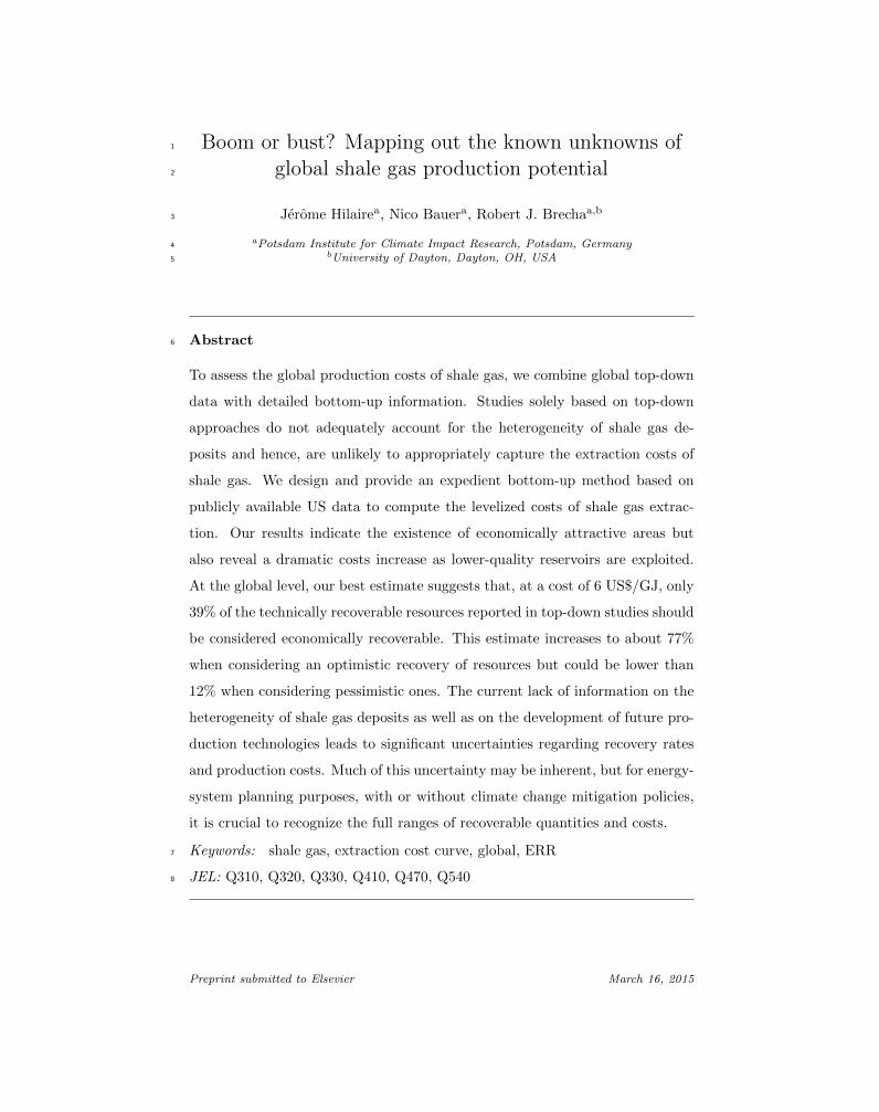
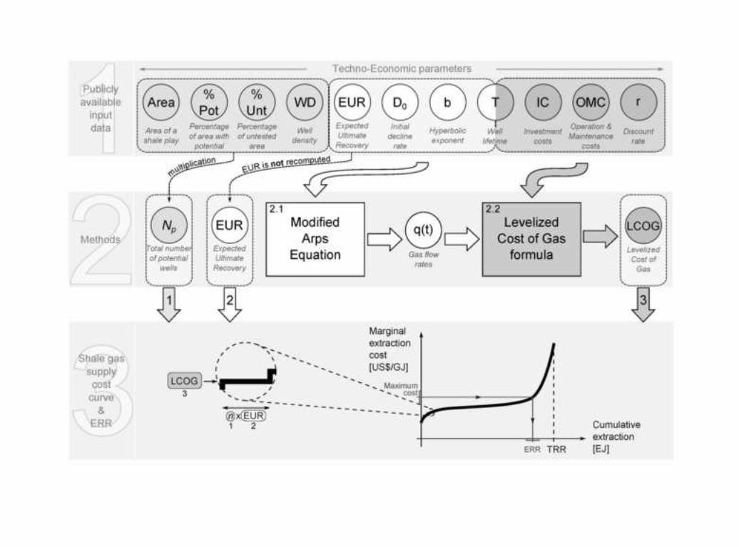
The methodology to compute a CECF is depicted in Figure 1. We start94

with a careful review of the grey and peer-reviewed literature that gives us an95

indication of the paucity of data and an overview of methods used by various96

communities - including academia, industry, NGO ... - to estimate shale gas97

extraction costs. We then design a comprehensive approach that accounts for98

4

the limits and uncertainties of available data. This enables us to compute US99

shale gas CECFs and importantly, include uncertainties. The main aspects of100

this approach are presented in the following paragraphs. For a more detailed101

description of methods and data, the reader is invited to consult the supple-102

mentary online material.103

1Publicly

available

input

data

Techno-Economic parameters

3Shale gas

supply

cost

curve

&

ERR

TRR

Marginal

extraction

cost

[US$/GJ]

Cumulative

extraction

[EJ]

LCOG

n x EUR

Maximumcost

ERR

3

1 2

2Methods

Levelized

Cost of Gas

formula

q(t)

Gas flow

rates

Modified

Arps

Equation

2.1 2.2

EUR is not recomputed

m

ultiplication

1 2 3

Figure 1: Flow diagram of the methodology employed in the computed tool. Note that EURdata are used in the Modified Arps’ equation as well as directly in the cumulative extractioncost curve.

104

We first collect and harmonise data for 11 techno-economic parameters that are105

repeatedly reported in the literature (Block 1 in Figure 1). These parameters106

are divided into 3 categories corresponding to 3 methods required to obtain a107

CECF. The first category contains 4 parameters coloured in light grey: Area108

(A), percentage of area with potential1 (%Pot), percentage of untested area2109

(%Unt) and well density (WD). These parameters are multiplied together to110

1Percent of area that is expected to have technically recoverable resources (EIA, 2013a)2Percent of total wells left to be drilled (EIA, 2013a)

5

obtain the total number of potential wells (Np) in a shale play (p) (Equation 1111

and Method 2.1 in Figure 1)).112

Np = A× %Pot× %Unt×WD (1)

The next 4 techno-economic parameters in white consist of the Estimated Ul-113

timate Recovery (EUR), the hyperbolic factor (b), the initial decline rate (D0)114

and the well lifetime (T ). These are fed to an equation based on the original115

Arps’ equation to compute gas production over time q(t), which is a crucial in-116

termediate step to calculating shale gas production costs (Method 2.2 in Figure117

1).118

119

Using empirical data, Arps devised an equation that describes oil and gas pro-120

duction decline over time (Arps, 1944). Owing to its simplicity, this formula is121

still largely employed in the oil and gas industry, including by shale gas extrac-122

tion companies. Shale gas producers have observed that early gas production123

rates could be reasonably estimated with hyperbolic decline type curves. The124

hyperbolic form of the Arps equation leads however to infinitely decreasing de-125

cline rates and requires the inclusion of additional parameters such as well life126

time to avoid overestimating future production.127

128

Despite continuous debate over the accuracy of the Arps equation, no alterna-129

tive method has yet proven to be superior in predicting gas production. Though130

a promising one recently proposed by Patzek et al. (2013) might turn out to131

be more useful in the future3, most published data currently relate to the Arps132

equation and so we use this well-established and expedient method here.133

134

3Patzek et al. (2013) developed a stylized physical model of a multi-stage hydraulic frac-tured horizontal shale gas well. With the help of gas production data of more than 8000 UShorizontal wells over 10 years, they employed their model to devise a 2-stage equation thatdescribed gas production over time. The early transient flow regime is modelled by a scalingcurve that is proportional to the inverse of the square root of time. The later boundary flowregime that starts after the so-called interference time is estimated with a simple exponentialdecline curve.

6

In its original form the hyperbolic Arps equation states that gas production135

is a function of initial gas production q0 and that it follows a hyperbolic decline136

over time. However, for lack of reported q0 data, we replace q0 by better re-137

ported parameters and effectively modify the Arps equation. In particular EUR138

can be obtained from integrating q(t) over T so we substitute q0 by a function139

of EUR, b, D0 and T to calculate q(t) (See supplementary online material for140

calculation details). This approach enables us to find the unique gas production141

rates q(t) that are consistent with the parameter values of EUR, b, D0 and T .142

The modified equation reads:143

q(t) =EUR (b−1)D0

(1+bD0T )(b−1)/b−1

(1 + bD0t)1/b

(2)

144

Next, gas production rates q(t) are combined with Investment Costs (IC), Op-145

eration and Maintenance Costs (OMC), a discount rate (r) and well lifetime146

(T ) to compute the levelized costs of gas (LCOG). The LCOG formula is bor-147

rowed from the field of economics and provides the unit costs of producing shale148

gas over the lifetime of a well (Equation 3 and Method 2.3 in Figure 1).149

LCOG =IC +

∑Tt=0

q(t)OMC

(1+r)t∑Tt=0

q(t)

(1+r)t

(3)

150

151

Finally, we combine the above equations 1, 2 and 3 to construct a CECF. For152

each play p, EUR probability distributions (Pp(EUR)) are multiplied by the153

total number of potential wells (Np) to identify the number of wells (n) which154

will produce a certain EUR. Sorting then the LCOG of all potential shale gas155

wells in ascending order and combining them with their associated EUR and the156

number of potential wells n yield a cumulative extraction cost function of shale157

gas (Block 3 in Figure 1). Technically Recoverable Resources (TRR), a metric158

common to many shale gas assessment studies, can be obtained by summing159

the EUR of all total potential wells across all shale plays P (Equation 4). In160

7

addition, economic recoverable resources (ERR) can be inferred from the curve161

for any given cost threshold.162

TRR =

P∑p=1

Np × Pp(EUR) × EUR (4)

163

164

165

2.3. Uncertainty166

Techno-economic estimates bear large uncertainties. Those can be partly167

explained by the lack of in situ data but in this study they also stem from a168

lack of public data availability. To test the sensitivity of our results to these un-169

certainties we define lower, best and upper estimates for the 11 techno-economic170

parameters considered in this analysis. The best estimate for the EUR param-171

eter is the result of combining the distributional data from USGS (2012) and172

EIA (2013a) with estimates of Area, well density in those same references. We173

then apply a ±50% change in EUR to define the lower and upper estimates4174

as in (EIA, 2013a). The lower, best and upper estimates of the other param-175

eters including b, D0, T , IC, OMC, r are based on our literature review (See176

supplementary online material for more information). When several estimates177

are available we define the best estimate as the mean, the lower estimate as the178

minimum value and the upper estimate as the maximum value. For some shale179

gas play data could nonetheless not be retrieved. In this case, the best estimate180

is simply the mean across all currently available data (See Table 1).181

182

At the global scale, an additional level of uncertainty on TRR needs to be taken183

into account for the global CECF. We compile the most recent world TRR es-184

timates from Rogner et al. (2012); Pearson et al. (2012); McGlade et al. (2013);185

EIA (2013b) and define best, lower and upper estimates accordingly. We also186

4Note that these sensitivity factors are not supposed to reflect uncertainty but are usedallow discussion.

8

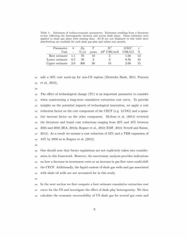
Table 1: Estimates of techno-economic parameters. Estimates resulting from a literaturereview reflecting the heterogeneity between and across shale plays. These estimates wereapplied to shale gas plays with missing data. EUR are not displayed in this table sincedistributions are available for each shale gas play and values vary greatly.

Parameter b D0 T IC OMC rUnit - %/yr years 106 US$/well US$/GJ %

Best estimate 1.1 70 10 5 1.00 12Lower estimate 0.5 50 2 3 0.50 10Upper estimate 2.0 300 30 10 2.00 15

add a 50% cost mark-up for non-US regions (Deutsche Bank, 2011; Pearson187

et al., 2012).188

189

The effect of technological change (TC) is an important parameter to consider190

when constructing a long-term cumulative extraction cost curve. To provide191

insights on the potential impacts of technological innovation, we apply a cost192

reduction factor on the cost component of the CECF (e.g. LCOG) and a quan-193

tity increase factor on the other component. McJeon et al. (2014) reviewed194

the literature and found cost reductions ranging from 20% and 45% between195

2035 and 2050 (IEA, 2012a; Rogner et al., 2012; EMF, 2013; Newell and Raimi,196

2014). As a result we assume a cost reduction of 33% and a TRR expansion of197

44% by 2050 as in Rogner et al. (2012).198

199

One should note that future regulations are not explicitely taken into consider-200

ation in this framework. However, the uncertainty analysis provides indications201

on how a decrease in investment costs or an increase in gas flow rates could shift202

the CECF. Additionally, the liquid content of shale gas wells and gas associated203

with shale oil wells are not accounted for in this study.204

205

In the next section we first compute a best estimate cumulative extraction cost206

curve for the US and investigate the effect of shale play heterogeneity. We then207

calculate the economic recoverability of US shale gas for several gas costs and208

9

draw conclusions regarding shale gas availability at the global scale.209

3. Results and discussion210

3.1. US shale gas extraction costs211

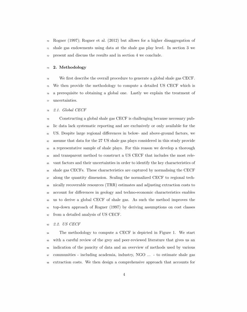
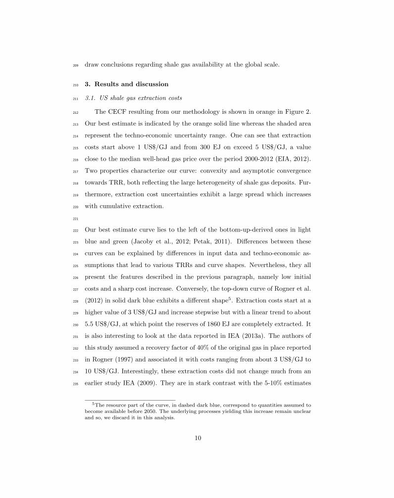
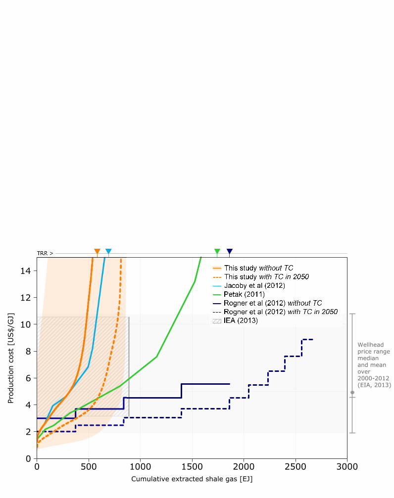
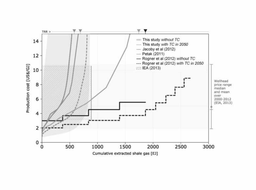
The CECF resulting from our methodology is shown in orange in Figure 2.212

Our best estimate is indicated by the orange solid line whereas the shaded area213

represent the techno-economic uncertainty range. One can see that extraction214

costs start above 1 US$/GJ and from 300 EJ on exceed 5 US$/GJ, a value215

close to the median well-head gas price over the period 2000-2012 (EIA, 2012).216

Two properties characterize our curve: convexity and asymptotic convergence217

towards TRR, both reflecting the large heterogeneity of shale gas deposits. Fur-218

thermore, extraction cost uncertainties exhibit a large spread which increases219

with cumulative extraction.220

221

Our best estimate curve lies to the left of the bottom-up-derived ones in light222

blue and green (Jacoby et al., 2012; Petak, 2011). Differences between these223

curves can be explained by differences in input data and techno-economic as-224

sumptions that lead to various TRRs and curve shapes. Nevertheless, they all225

present the features described in the previous paragraph, namely low initial226

costs and a sharp cost increase. Conversely, the top-down curve of Rogner et al.227

(2012) in solid dark blue exhibits a different shape5. Extraction costs start at a228

higher value of 3 US$/GJ and increase stepwise but with a linear trend to about229

5.5 US$/GJ, at which point the reserves of 1860 EJ are completely extracted. It230

is also interesting to look at the data reported in IEA (2013a). The authors of231

this study assumed a recovery factor of 40% of the original gas in place reported232

in Rogner (1997) and associated it with costs ranging from about 3 US$/GJ to233

10 US$/GJ. Interestingly, these extraction costs did not change much from an234

earlier study IEA (2009). They are in stark contrast with the 5-10% estimates235

5The resource part of the curve, in dashed dark blue, correspond to quantities assumed tobecome available before 2050. The underlying processes yielding this increase remain unclearand so, we discard it in this analysis.

10

reported in Sandrea (2012). In this analysis, 65% of shale gas resources can be236

economically recovered at 6 US$/GJ but this value we decreases to 19% at 3237

US$/GJ. Clearly, the heterogeneity of shale gas deposits is not reflected in the238

outcomes of these top-down studies which could lead to a misrepresentation of239

extraction costs, as well as larger TRR estimates.240

241

As expected technological change induces a shift rightward and downward of242

the CECFs. Nonetheless the differences observed in the previous paragraph243

between bottom-up and top-down studies are still present. Our best estimate244

becomes cheaper than the CECF in Petak (2011) for the first 600 EJ but still245

exhibits a steep cost increase after it. The CECF that accounts for technologi-246

cal change in Rogner et al. (2012) still misses cheap deposits and the steep cost247

increase because of the small number of categories.248

249

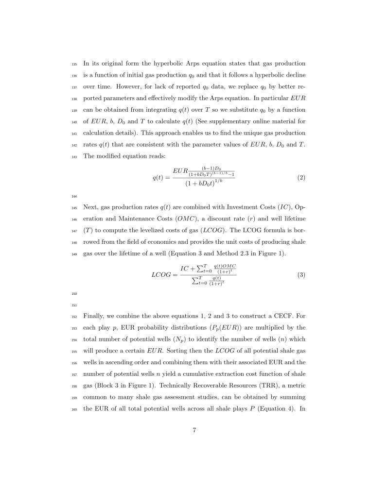
As a means of harmonizing the six different results shown in Fig. 2, we nor-250

malize the cumulative extraction cost curves, thereby identifying the fraction251

of assumed TRR that can be economically recovered at a given cost (Fig. 3).252

Differences between all bottom-up curves have faded out to a large extent. Our253

results are more optimistic between 4.5 and 6.5 US$/GJ but our middle curve254

remains within a distance of 20% from the other two. On the contrary, discrep-255

ancies between bottom-up and top-down curves are emphasized on this figure.256

The linear assumption and small number of categories in the top-down study257

is clearly at odds with the exponential increase in bottom-up studies. The two258

curves accounting for technological change are close to each other for production259

costs ranging between 3-6 US$/GJ but the top-down curve does not account for260

the cheap deposits and the steep cost increase.261

262

Given the relatively robust shape of bottom-up curves, we further perform a263

regression on our curve with a 3rd order polynomial in order to facilitate the264

estimation of ERR and the use of the CECF in future studies. (Details are given265

in the supplementary online material) Not only can this equation be employed266

11

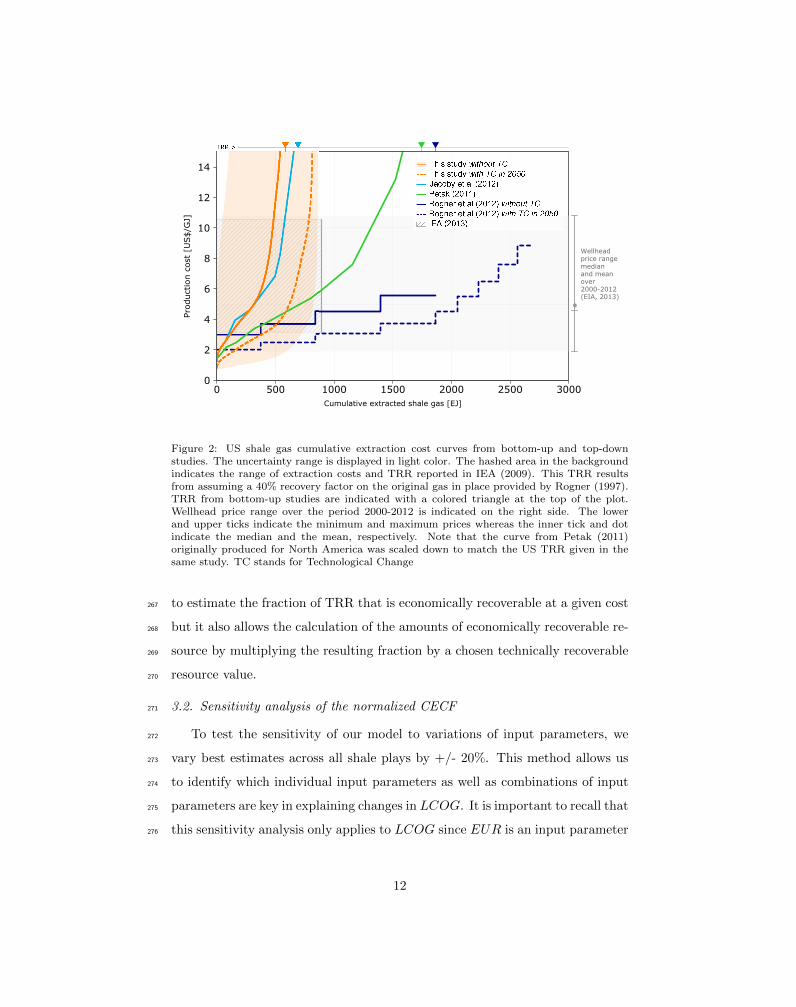
Figure 2: US shale gas cumulative extraction cost curves from bottom-up and top-downstudies. The uncertainty range is displayed in light color. The hashed area in the backgroundindicates the range of extraction costs and TRR reported in IEA (2009). This TRR resultsfrom assuming a 40% recovery factor on the original gas in place provided by Rogner (1997).TRR from bottom-up studies are indicated with a colored triangle at the top of the plot.Wellhead price range over the period 2000-2012 is indicated on the right side. The lowerand upper ticks indicate the minimum and maximum prices whereas the inner tick and dotindicate the median and the mean, respectively. Note that the curve from Petak (2011)originally produced for North America was scaled down to match the US TRR given in thesame study. TC stands for Technological Change

to estimate the fraction of TRR that is economically recoverable at a given cost267

but it also allows the calculation of the amounts of economically recoverable re-268

source by multiplying the resulting fraction by a chosen technically recoverable269

resource value.270

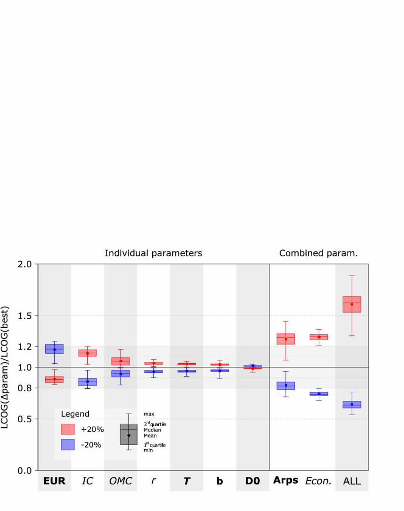
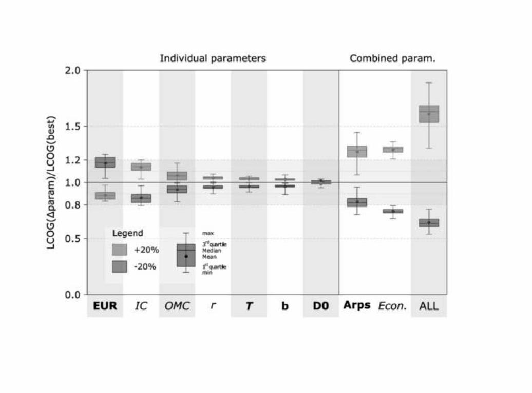
3.2. Sensitivity analysis of the normalized CECF271

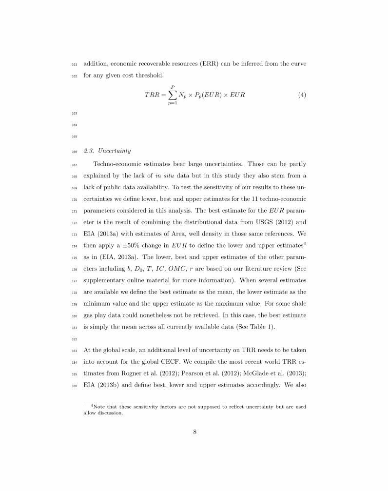
To test the sensitivity of our model to variations of input parameters, we272

vary best estimates across all shale plays by +/- 20%. This method allows us273

to identify which individual input parameters as well as combinations of input274

parameters are key in explaining changes in LCOG. It is important to recall that275

this sensitivity analysis only applies to LCOG since EUR is an input parameter276

12

Production costs [US$/GJ]

Figure 3: Economically recoverable fraction of TRR. Same as for Fig. 2.

in our framework. Changes in LCOG are defined as the ratio between LCOGs277

resulting from a change in input parameters and LCOGs resulting from the best-278

estimate case. These changes are summarised in box plots and shown on Figure279

4. Regarding individual parameters, it turns out that EUR, IC and OMC have280

the largest effects on LCOG, though they mostly remain below +/- 20%. As for281

combinations of input parameters, the effect of economic parameters is larger282

than 20% and dominates over that of Arps parameters. Nonetheless combining283

all input parameter sensitivities result in LCOG changes ranging between -20%284

and +80%, far greater than the effects of economic parameters alone. It is also285

important to note that these effects vary along the CECF as indicated by the286

box plots. In particular, the effect of OMC is reduced at higher costs. Given287

the relatively small effect of b, D0 and T , the results suggest that q0 has a large288

impact on LCOG.289

13

Figure 4: Sensitivity analysis of the normalized CECF. Economic parameters are in italicletters whereas non-economic parameters are in bold letters. The effect of single parametersis shown in the left panel. Combinations of parameters are displayed on the right panel.

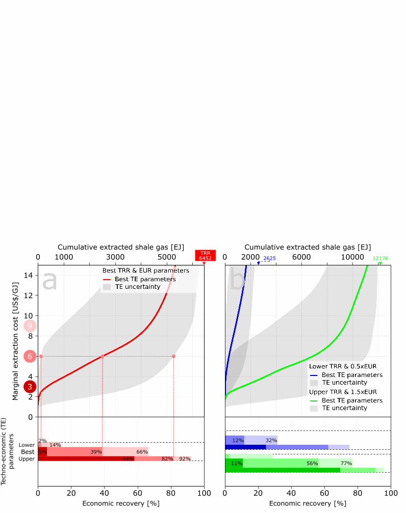
3.3. Global shale gas extraction costs290

Since shale gas activities outside the US are still in their infancy, detailed291

techno-economic data are not yet publicly available. As an alternative, one may292

gain insights at the global scale by scaling up the US shale gas CECF using293

global TRR estimates. Global TRRs have been estimated and recently com-294

piled by Pearson et al. (2012) and McGlade et al. (2013). In the present study295

we complete this dataset with other recent estimates from Rogner et al. (2012)296

and EIA (2013b). We compute a best estimate of about 6500 EJ and lower and297

upper estimates of about 2600 EJ and 12100 EJ, respectively (Details on these298

calculations can be found in the supplementary online material).299

300

In this last result section, we apply the previously computed normalized US301

curve to TRR estimates to obtain a global cumulative extraction cost curve. To302

make this extrapolation a bit more realistic, we apply a 50% cost mark-up to303

14

Techno-e

conom

ic (

TE)

para

mete

rs

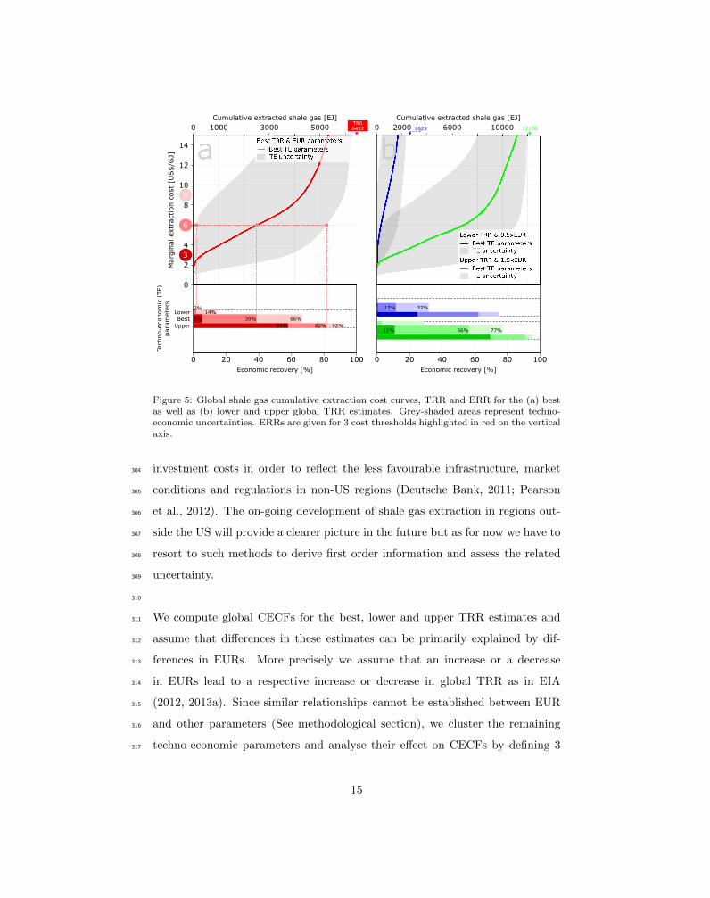
Figure 5: Global shale gas cumulative extraction cost curves, TRR and ERR for the (a) bestas well as (b) lower and upper global TRR estimates. Grey-shaded areas represent techno-economic uncertainties. ERRs are given for 3 cost thresholds highlighted in red on the verticalaxis.

investment costs in order to reflect the less favourable infrastructure, market304

conditions and regulations in non-US regions (Deutsche Bank, 2011; Pearson305

et al., 2012). The on-going development of shale gas extraction in regions out-306

side the US will provide a clearer picture in the future but as for now we have to307

resort to such methods to derive first order information and assess the related308

uncertainty.309

310

We compute global CECFs for the best, lower and upper TRR estimates and311

assume that differences in these estimates can be primarily explained by dif-312

ferences in EURs. More precisely we assume that an increase or a decrease313

in EURs lead to a respective increase or decrease in global TRR as in EIA314

(2012, 2013a). Since similar relationships cannot be established between EUR315

and other parameters (See methodological section), we cluster the remaining316

techno-economic parameters and analyse their effect on CECFs by defining 3317

15

parameter combinations best, lower and upper cases that span the range of318

possibilities (See online supplementary online material). In addition, for each319

of the three global CECFs, we provide estimates of economic recoverability6 at320

three different cost thresholds that pertain to the range of US wellhead prices321

between 2000 and 20127: 3, 6, and 9US$/GJ. To sum up, we perform an ex-322

tensive sensitivity analysis of economic recoverability along three dimensions:323

TRR and EUR, techno-economic parameters and costs.324

325

Let us first focus on the global CECF corresponding to the best TRR esti-326

mate and indicated by a red line on Figure 5(a). The associated economic327

recoverability is shown in the lower panel. At 6 US$/GJ, 39% of the TRR328

is economically recoverable which contrasts with the entire shale gas reserves329

that can be extracted in Rogner et al. (2012). The large uncertainties in input330

techno-economic data (grey area) change the recoverability at a cost of US$6/GJ331

to 2% and 82% in the lower and upper cases respectively, highlighting the need332

for better reporting of these parameters. Sensitivity to costs is also substantial.333

At 3 US$/GJ economic recoverability decreases to 5% whereas at 9 US$/GJ it334

increases to 66%, emphasizing the large impact of future gas prices on economic335

recovery.336

337

When the TRR and EUR uncertainty is accounted for economic recoverabil-338

ity is further impacted (Fig. 5(b)). One may first notice the important gap of339

about 10 ZJ between the blue and green curves that correspond to the lower340

and upper TRR and EUR cases. This reflects the lack of knowledge about shale341

gas plays inside and outside the US. The two curves exhibit the same insights342

gathered in the best TRR and EUR case. An additional interesting result is343

the decreasing incremental quantity available from moving from 3 US$/GJ to344

6defined as ERR/TRR7Wellhead price throughout the 1980s and 1990s was about $2. This was followed by a

large upward swing from 2000-2007 and then a downward trend. http://www.eia.gov/dnav/

ng/hist/n9190us3a.htm

16

6 US$/GJ and from 6 US$/GJ to 9 US$/GJ. This diminishing returns effect is345

the result of the shape of the CECFs.346

347

It is interesting to put these estimates into perspective. On the one hand, Henry348

Hub natural gas prices are currently around 4 US$/GJ and are projected to in-349

crease in the future (EIA, 2014). On the other hand, the US had produced about350

50 EJ of shale gas by the end of 2013 (EIA, 2014). These facts invalidate some351

of the CECFS. In particular those resting from lower techno-economic estimates352

and especially in the lower TRR & 0.5xEUR case. It is however worthwhile to353

note that all best techno-economic estimates at 6 US$/GJ which range between354

300 EJ and 6800 EJ are in agreement with current shale gas production.355

4. Conclusion356

In this study, we developed a method based on publicly available data that357

enables us to compute cumulative extraction cost curves of shale gas, derive358

economic recoverability and identify key uncertainties. We offer this method359

in the form of a computing tool8 and also provide 3rd order polynomial fitting360

curves that can be applied to estimates of technically recoverable resources to361

quickly approximate shale gas extraction costs. Our results are found to be in362

good agreement with previous bottom-up studies and highlight the importance363

of accounting for the heterogeneity of shale gas deposits in estimating extraction364

costs. Crucially, our results show that extraction costs are likely not adequately365

represented in previously published top-down studies. More importantly we366

identified initial production, iunvestment costs, and operation and maintenance367

costs as key parameters driving differences in estimates of the levelized costs of368

gas. It is also interesting to note that Arps parameters describing gas flow over369

time have a lesser impact on overall costs than economic ones (e.g. investment370

costs, operation and maintenance costs, and discount rate).371

372

8Please send an e-mail to hilaire@pik-potsdam.de

17

For the US, we calculated that about 400 EJ or two thirds of technically recover-373

able resources could be economically recovered at a cost of 6 US$/GJ in the best374

estimate case. This estimate decreases dramatically to 100 EJ at 3 US$/GJ,375

a result that is still in agreement with current production. At the global level376

and at 6 US$/GJ, we obtain economically recoverable resources ranging be-377

tween 300 EJ and 6800 EJ in the case of best techno-economic estimates. It378

is worthwhile to note that the extrapolation of detailed US data to the global379

level, even when including a +50% mark-up on investment costs, cannot fully380

account for the different techno-economic characteristics of other regions. As381

drilling activity starts to take place outside the US and new data will become382

available, estimates could be refined.383

384

Since data availability is an important factor that determines the outcome of385

such analysis, it is necessary to address its scarcity to refine estimates in the386

future. Although the results from this analysis can only be as accurate as the387

information and the assumptions upon which it draws, they suggest that anal-388

yses at the global level and over the 21st century using estimates reported in389

top-down studies could overestimate the future of gas production. This could390

have important repercussions on both climate change mitigation strategies and391

energy security and access.392

Acknowledgments393

We would like to thank Austin Mitchell (Carnegie Mellon University) and El-394

mar Kriegler (Potsdam Institute for Climate Impact Research) for valuable com-395

ments and stimulating discussions. Our thanks go also to the two anonymous396

reviewers for their useful comments and suggestions to improve this manuscript.397

We are very grateful to Hans-Holger Rogner who provided us with US shale gas398

data from the Global Energy Assessment. Funding from the German Federal399

Ministry of Education and Research (BMBF) in the call ”Okonomie des Kli-400

mawandels” (funding code 01LA11020B/Green Paradox) is gratefully acknowl-401

edged.402

18

References403

Arps, J.J., 1944. Analysis of decline curves. Petroleum Technology .404

BGR, 2009. Reserven, Ressourcen, Verfgbarkeit. Annual Report. Federal Insti-405

tute for Geoscience and Natural Resources (BGR). Hannover, Germany.406

BGR, 2011. Reserves, Resources and Availability of Energy Resources. An-407

nual Report. Federal Institute for Geoscience and Natural Resources (BGR).408

Hannover, Germany.409

BP, 2013. BP Energy Outlook 2030. Technical Report. British Petroleum.410

URL: http://www.bp.com/content/dam/bp/pdf/Energy-economics/411

Energy-Outlook/BP_Energy_Outlook_Booklet_2013.pdf.412

Deutsche Bank, 2011. European gas: A first look at EU shale-gas prospects.413

EIA, 2011. World Shale Gas Resources: An Initial Assessment of 14 Regions414

Outside the United States. Technical Report. Energy Information Adminis-415

tration. Washington DC.416

EIA, 2012. Annual Energy Outlook 2012 with Projection to 2035. Techni-417

cal Report DOE/EIA-0383(2012). U.S. Energy Information Administration.418

Washington, DC, USA.419

EIA, 2013a. Annual Energy Outlook 2013 with Projection to 2040. Techni-420

cal Report DOE/EIA-0383(2013). U.S. Energy Information Administration.421

Washington, DC, USA.422

EIA, 2013b. Technically Recoverable Shale Oil and Shale Gas Resources: An As-423

sessment of 137 Shale Formations in 41 Countries Outside the United States.424

Technical Report. U.S. Energy Information Administration. U.S. Department425

of Energy, Washington, DC 20585, USA.426

EIA, 2014. Annual Energy Outlook 2014 with Projection to 2040. Techni-427

cal Report DOE/EIA-0383(2013). U.S. Energy Information Administration.428

Washington, DC, USA.429

19

EMF, 2013. Changing the game? Emissions and Market Implications of New430

Natural Gas Supplies. Technical Report. Energy Modelling Forum. Stanford431

University, Stanford, California, USA. URL: https://web.stanford.edu/432

group/emf-research/docs/emf26/Summary26.pdf.433

IEA, 2009. World Energy Outlook. Technical Report. International Energy434

Agency (IEA). Paris, France.435

IEA, 2011. World Energy Outlook. Technical Report. International Energy436

Agency (IEA). Paris, France.437

IEA, 2012a. Golden Age of Gas. Technical Report. International Energy Agency438

(IEA). Paris, France.439

IEA, 2012b. World Energy Outlook. Technical Report. International Energy440

Agency (IEA). Paris, France.441

IEA, 2013a. Resources to Reserves. Technical Report. International Energy442

Agency (IEA). Paris, France.443

IEA, 2013b. World Energy Outlook. Technical Report. International Energy444

Agency (IEA). Paris, France.445

Ikonnikova, S., Browning, J., Gulen, G., Smye, K., Tinker, S., 2015. Factors446

influencing shale gas production forecasting: Empirical studies of barnett,447

fayetteville, haynesville, and marcellus shale plays. Economics of Energy &448

Environmental Policy 4. doi:dx.doi.org/10.5547/2160-5890.4.1.siko.449

Jacoby, H.D., O’Sullivan, F.M., Paltsev, S., 2012. The influence of shale gas on450

U.S. energy and environmental policy. Economics of Energy & Environmental451

Policy 1. URL: http://dx.doi.org/10.5547/2160-5890.1.1.5.452

McCollum, D., Bauer, N., Calvin, K., Kitous, A., Riahi, K., 2014. Fos-453

sil resource and energy security dynamics in conventional and carbon-454

constrained worlds. Climatic Change 123. URL: http://dx.doi.org/10.455

1007/s10584-013-0939-5.456

20

McGlade, C., Speirs, J., Sorrell, S., 2013. Unconventional gas - a review of457

regional and global resource estimates. Energy 55, 571–584.458

McJeon, H., Edmonds, J., Bauer, N., Clarke, L., Fisher, B., Flannery, B.P.,459

Hilaire, J., Krey, V., Marangoni, G., Mi, R., Riahi, K., Rogner, H., Tavoni,460

M., 2014. Limited impact on decadal-scale climate change from increased use461

of natural gas. Nature 514.462

Nakano, J., Pumphrey, D., Price Jr., R., Walton, M.A., 2012. Prospects for463

Shale Gas Development in Asia: Examining potentials and challenges in464

China and India. Technical Report. Center for Strategic and International465

Studies (CSIS). Washington, DC.466

Newell, R.G., Raimi, D., 2014. Implications of shale gas development for climate467

change. Environ. Sci. Technol. 48, 83608368.468

Patzek, T.W., Male, F., Marder, M., 2013. Gas production in the barnett469

shale obeys a simple scaling theory. Proceedings of the National Academy of470

Sciences URL: http://www.pnas.org/cgi/doi/10.1073/pnas.1313380110.471

Pearson, I.L.G., Zeniewski, P., Gracceva, F., Zastera, P., McGlade, C., Sorrell,472

S., Speirs, J., Thonhauser, G., Alecu, C., Eriksson, A., Schuetz, M., Toft, P.,473

2012. Unconventional Gas: Potential Energy Market Impacts in the Euro-474

pean Union. JRC Scientific and Policy Report EU R 25305 EN. European475

Commission, Joint Research Centre, Institute for Energy and Transport. Wes-476

terduinweg 3, 1755 LE, Petten, The Netherlands. URL: http://ec.europa.477

eu/dgs/jrc/downloads/jrc_report_2012_09_unconventional_gas.pdf.478

Petak, K.R., 2011. Impact of natural gas supply on CHP deployment, in: US479

Clean Heat & Power Association’s (USCHPA), Spring CHP Forum, Wash-480

ington, DC.481

Richter, P., 2015. From boom to bust? a critical look at us shale gas projections.482

Economics of Energy & Environmental Policy 4.483

21

Rogner, H.H., 1997. An assessment of world hydrocarbon resources.484

Annual Review of Energy and the Environment 22, 217–262. URL:485

http://arjournals.annualreviews.org/doi/abs/10.1146%2Fannurev.486

energy.22.1.217, doi:10.1146/annurev.energy.22.1.217.487

Rogner, H.H., Aguilera, R.F., Archer, C.L., Bertani, R., Bhattacharya, S.,488

Dusseault, M.B., Gagnon, L., Haberl, H., Hoogwijk, M., Johnson, A., Rogner,489

M.L., Wagner, H., Yakushev, V., 2012. Energy resources and potentials, in:490

Global Energy Assessment - Toward a Sustainable Future. Cambridge Uni-491

versity Press.492

Sandrea, R., 2012. Evaluating production potential of mature us oil, gas shale493

plays. Oil & Gas Journal .494

Trembath, A., Jenkins, J., Nordhaus, T., Shellenberger, M., 2012. Where the495

Shale Gas Revolution Came From: Government’s role in the development496

of hydraulic fracturing in shale. Technical Report. Breakthrough Institute.497

Oakland, CA, USA.498

USGS, 2000. World Petroleum Assessment. Technical Report. US Geological499

Survey. Washington, DC.500

USGS, 2012. Variability of Distributions of Well-Scale Estimated Ultimate Re-501

covery for Continuous (Unconventional) Oil and Gas Resources in the United502

States. Technical Report. U.S. Geological Survey. U.S. Geological Survey,503

Reston, Virginia, USA.504

Wang, Z., Krupnick, A., 2013. A restrospective review of shale gas development505

in the united states. what led to the boom? Resources for the Future, Dis-506

cussion Paper URL: http://www.rff.org/RFF/documents/RFF-DP-13-12.507

pdf.508

22

LaTeX Source FilesClick here to download LaTeX Source Files: LaTeX source files.zip

1Publicly

available

input

data

Techno-Economic parameters

3Shale gas

supply

cost

curve

&

ERR

TRR

Marginal

extraction

cost

[US$/GJ]

Cumulative

extraction

[EJ]

LCOG

n x EUR

Maximumcost

ERR

3

1 2

2Methods

Levelized

Cost of Gas

formula

q(t)

Gas flow

rates

Modified

Arps

Equation

2.1 2.2

EUR is not recomputed

m

ultiplication

1 2 3

Figure(s)

Figure(s)

Production costs [US$/GJ]

Figure(s)

Figure(s)

Techno-e

conom

ic (

TE)

para

mete

rs

Figure(s)

Figure(s)Click here to download high resolution image

Figure(s)Click here to download high resolution image

Figure(s)Click here to download high resolution image

Figure(s)Click here to download high resolution image

Figure(s)Click here to download high resolution image

Boom or Bust? Mapping out the known

unknowns of global shale gas production

potential

Supplementary material

Jérôme Hilaire, Nico Bauer and Robert J. Brecha

Contents Modified Arps equation .......................................................................................................................... 3

Data, input parameters and assumptions ............................................................................................... 3

Technically recoverable resources (TRR) ............................................................................................ 3

Africa (sub-saharan) ........................................................................................................................ 6

Australia .......................................................................................................................................... 6

Canada ............................................................................................................................................. 6

China ................................................................................................................................................ 7

Central and South America ............................................................................................................. 7

Eastern Europe ................................................................................................................................ 7

Former Soviet Union ....................................................................................................................... 8

India ................................................................................................................................................. 8

Middle East and North Africa .......................................................................................................... 9

Other developing Asia ..................................................................................................................... 9

USA .................................................................................................................................................. 9

Western Europe ............................................................................................................................ 10

Area (A), Percentage of Potential Area (%Pot), Percentage of Untested Area (%Unt)..................... 10

Well drainage, well spacing and well density (WD) .......................................................................... 10

Estimated ultimate recovery (EUR) ................................................................................................... 10

Initial decline rate (D0) ....................................................................................................................... 11

Hyperbolic exponent (b) .................................................................................................................... 12

Investment costs (IC) ......................................................................................................................... 12

Operation and Maintenance costs (OMC) ........................................................................................ 12

Discount rate (r) ................................................................................................................................ 13

Well’s lifetime (T) .............................................................................................................................. 13

Supplementary online material

Sensitivity analysis ................................................................................................................................. 13

Sensitivity to modified Arps parameters ........................................................................................... 14

Sensitivity to LCOG parameters ........................................................................................................ 15

CECF regressions ................................................................................................................................... 16

Unit conversion ..................................................................................................................................... 16

Glossary ................................................................................................................................................. 16

Model parameters and variables ...................................................................................................... 16

Institutions ........................................................................................................................................ 17

References ............................................................................................................................................. 17

Appendix A: Investment Costs estimates .............................................................................................. 18

Modified Arps equation

In this section we show how we derive the numerator of the modified Arps equation.

1 ⁄

1

1 ⁄

We pose 1 . As a result we obtain .

The equation then becomes:

1 ⁄

We know that , if 1. Thus we obtain the following equation:

!"/ $ 1/%

1 &"/ $ 1

$ 1

Hence

$ 11 &"/ $ 1

Data, input parameters and assumptions

In this section, we provide further information about data used and assumptions made in our

methodology. All data, algorithms and code are available from the authors upon request. The

equations presented in our study are repeated here:

'( ) *%,- *% *. (1)

$ 11 &" ⁄ $ 1

1 ⁄

(2)

/01 ∑34 051 6778∑ 1 6778

(3)

& 9'( * ,( * :

(8

(4)

Technically recoverable resources (TRR)

TRR can be calculated over different geographical areas and is mainly reported for countries. For

instance US estimates range between 509 EJ and 1863 EJ (see Table 1). The best-estimate taken in

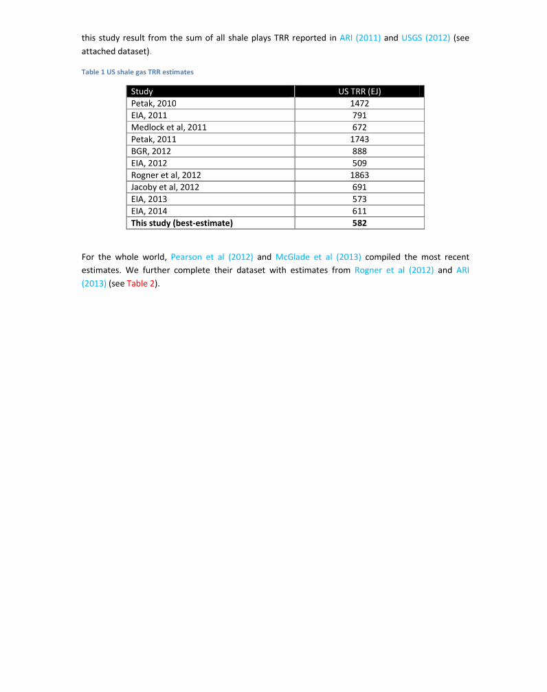
this study result from the sum of all shale plays TRR reported in ARI (2011) and USGS (2012) (see

attached dataset).

Table 1 US shale gas TRR estimates

Study US TRR (EJ)

Petak, 2010 1472

EIA, 2011 791

Medlock et al, 2011 672

Petak, 2011 1743

BGR, 2012 888

EIA, 2012 509

Rogner et al, 2012 1863

Jacoby et al, 2012 691

EIA, 2013 573

EIA, 2014 611

This study (best-estimate) 582

For the whole world, Pearson et al (2012) and McGlade et al (2013) compiled the most recent

estimates. We further complete their dataset with estimates from Rogner et al (2012) and ARI

(2013) (see Table 2).

Table 2 Global shale gas TRR

Technically Recoverable

Resources (EJ)

World regions and

countries Low Best High Sources

Africa (sub-saharan)* 411 457 512 McGlade et al (2013), Rogner et al (2012) and

ARI (2013)

Australia 149 341 461 McGlade et al (2013), Rogner et al (2012) and

ARI (2013)

Canada 133 412 1047 McGlade et al (2013), Rogner et al (2012) and

ARI (2013)

China 241 917 1336 McGlade et al (2013), Rogner et al (2012) and

ARI (2013)

Central and South

America**

149 1183 2084 McGlade et al (2013), Rogner et al (2012) and

ARI (2013)

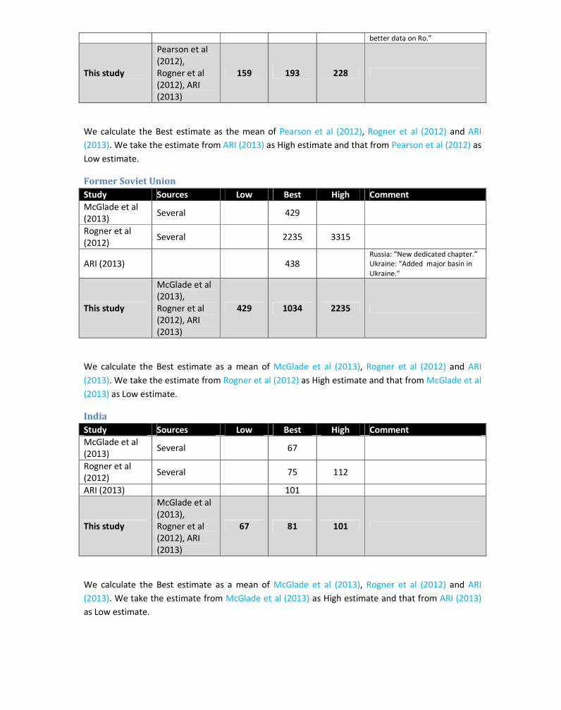
Eastern Europe 159 193 228 Pearson et al (2012), Rogner et al (2012) and

ARI (2013)

Former Soviet Union 429 1034 2235 McGlade et al (2013), Rogner et al (2012) and

ARI (2013)

India 67 81 101 McGlade et al (2013), Rogner et al (2012) and

ARI (2013)

Middle East and North

Africa 104 665 1062 McGlade et al (2013), Rogner et al (2012) and

ARI (2013)

Other developing Asia 48 271 818 McGlade et al (2013), Rogner et al (2012) and

ARI (2013)

USA 511 582 1863 McGlade et al (2013), Rogner et al (2012) and

ARI (2013)

Western Europe 224 316 429 Pearson et al (2012), Rogner et al (2012) and

ARI (2013)

TOTAL 2624 6454 12175

* In McGlade et al (2013), Africa included North Africa which was also accounted in Middle East. This

is why we discard this estimate.

** In this study, Mexico belongs to the Central and South America region.

The estimate taken from Rogner et al (2012) includes 20% of gas in place that are deemed to

become recoverable by 2050.

All estimates provided in this section are in exajoules (EJ) and have been converted (when required)

by using the unit conversion table in Rogner et al (2012) (Table 7.3, page 437).

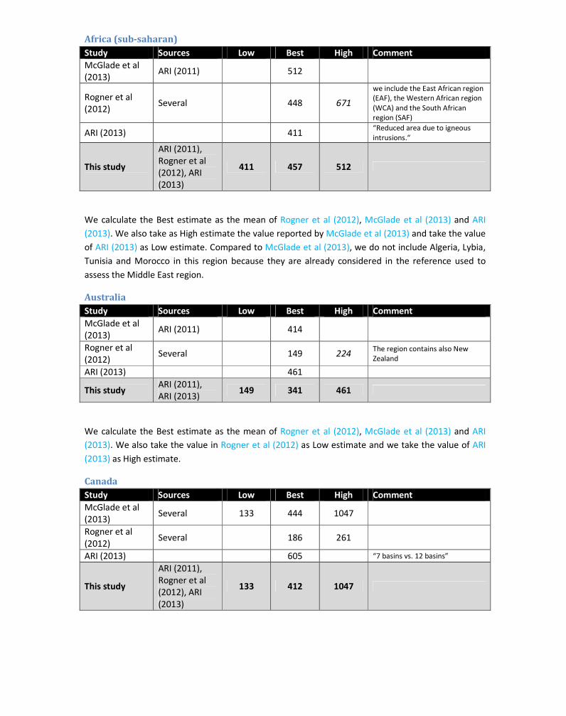
Africa (sub-saharan)

Study Sources Low Best High Comment

McGlade et al

(2013) ARI (2011) 512

Rogner et al

(2012) Several 448 671

we include the East African region

(EAF), the Western African region

(WCA) and the South African

region (SAF)

ARI (2013) 411 “Reduced area due to igneous

intrusions.“

This study

ARI (2011),

Rogner et al

(2012), ARI

(2013)

411 457 512

We calculate the Best estimate as the mean of Rogner et al (2012), McGlade et al (2013) and ARI

(2013). We also take as High estimate the value reported by McGlade et al (2013) and take the value

of ARI (2013) as Low estimate. Compared to McGlade et al (2013), we do not include Algeria, Lybia,

Tunisia and Morocco in this region because they are already considered in the reference used to

assess the Middle East region.

Australia

Study Sources Low Best High Comment

McGlade et al

(2013) ARI (2011) 414

Rogner et al

(2012) Several 149 224

The region contains also New

Zealand

ARI (2013) 461

This study ARI (2011),

ARI (2013) 149 341 461

We calculate the Best estimate as the mean of Rogner et al (2012), McGlade et al (2013) and ARI

(2013). We also take the value in Rogner et al (2012) as Low estimate and we take the value of ARI

(2013) as High estimate.

Canada

Study Sources Low Best High Comment

McGlade et al

(2013) Several 133 444 1047

Rogner et al

(2012) Several 186 261

ARI (2013) 605 “7 basins vs. 12 basins”

This study

ARI (2011),

Rogner et al

(2012), ARI

(2013)

133 412 1047

We calculate the Best estimate as the mean of Rogner et al (2012), McGlade et al (2013) and ARI

(2013). We keep the Low and High estimates as defined in McGlade et al (2013).

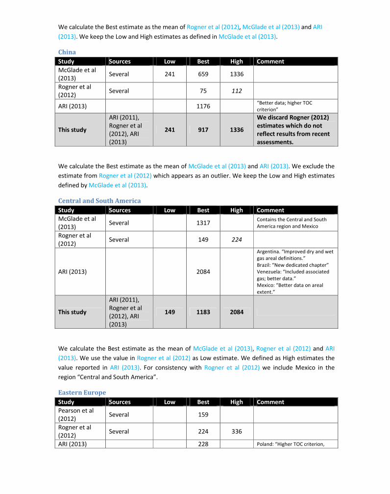
China

Study Sources Low Best High Comment

McGlade et al

(2013) Several 241 659 1336

Rogner et al

(2012) Several 75 112

ARI (2013) 1176 “Better data; higher TOC

criterion”

This study

ARI (2011),

Rogner et al

(2012), ARI

(2013)

241 917 1336

We discard Rogner (2012)

estimates which do not

reflect results from recent

assessments.

We calculate the Best estimate as the mean of McGlade et al (2013) and ARI (2013). We exclude the

estimate from Rogner et al (2012) which appears as an outlier. We keep the Low and High estimates

defined by McGlade et al (2013).

Central and South America

Study Sources Low Best High Comment

McGlade et al

(2013) Several 1317

Contains the Central and South

America region and Mexico

Rogner et al

(2012) Several 149 224

ARI (2013) 2084

Argentina. “Improved dry and wet

gas areal definitions.”

Brazil: “New dedicated chapter”

Venezuela: “Included associated

gas; better data.”

Mexico: “Better data on areal

extent.”

This study

ARI (2011),

Rogner et al

(2012), ARI

(2013)

149 1183 2084

We calculate the Best estimate as the mean of McGlade et al (2013), Rogner et al (2012) and ARI

(2013). We use the value in Rogner et al (2012) as Low estimate. We defined as High estimates the

value reported in ARI (2013). For consistency with Rogner et al (2012) we include Mexico in the

region “Central and South America”.

Eastern Europe

Study Sources Low Best High Comment

Pearson et al

(2012) Several 159

Rogner et al

(2012) Several 224 336

ARI (2013) 228 Poland: “Higher TOC criterion,

better data on Ro.”

This study

Pearson et al

(2012),

Rogner et al

(2012), ARI

(2013)

159 193 228

We calculate the Best estimate as the mean of Pearson et al (2012), Rogner et al (2012) and ARI

(2013). We take the estimate from ARI (2013) as High estimate and that from Pearson et al (2012) as

Low estimate.

Former Soviet Union

Study Sources Low Best High Comment

McGlade et al

(2013) Several 429

Rogner et al

(2012) Several 2235 3315

ARI (2013) 438 Russia: “New dedicated chapter.”

Ukraine: “Added major basin in

Ukraine.”

This study

McGlade et al

(2013),

Rogner et al

(2012), ARI

(2013)

429 1034 2235

We calculate the Best estimate as a mean of McGlade et al (2013), Rogner et al (2012) and ARI

(2013). We take the estimate from Rogner et al (2012) as High estimate and that from McGlade et al

(2013) as Low estimate.

India

Study Sources Low Best High Comment

McGlade et al

(2013) Several 67

Rogner et al

(2012) Several 75 112

ARI (2013) 101

This study

McGlade et al

(2013),

Rogner et al

(2012), ARI

(2013)

67 81 101

We calculate the Best estimate as a mean of McGlade et al (2013), Rogner et al (2012) and ARI

(2013). We take the estimate from McGlade et al (2013) as High estimate and that from ARI (2013)

as Low estimate.

Middle East and North Africa

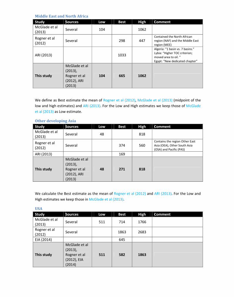
Study Sources Low Best High Comment

McGlade et al

(2013) Several 104 1062

Rogner et al

(2012) Several 298 447

Contained the North African

region (NAF) and the Middle East

region (MEE)

ARI (2013) 1033

Algeria: “1 basin vs. 7 basins.”

Lybia: “Higher TOC criterion;

moved area to oil. ”

Egypt: “New dedicated chapter”

This study

McGlade et al

(2013),

Rogner et al

(2012), ARI

(2013)

104 665 1062

We define as Best estimate the mean of Rogner et al (2012), McGlade et al (2013) (midpoint of the

low and high estimates) and ARI (2013). For the Low and High estimates we keep those of McGlade

et al (2013) as Low estimate.

Other developing Asia

Study Sources Low Best High Comment

McGlade et al

(2013) Several 48 818

Rogner et al

(2012) Several 374 560

Contains the region Other East

Asia (OEA), Other South Asia

(OSA) and Pacific (PAS)

ARI (2013) 169

This study

McGlade et al

(2013),

Rogner et al

(2012), ARI

(2013)

48 271 818

We calculate the Best estimate as the mean of Rogner et al (2012) and ARI (2013). For the Low and

High estimates we keep those in McGlade et al (2013).

USA

Study Sources Low Best High Comment

McGlade et al

(2013) Several 511 714 1766

Rogner et al

(2012) Several 1863 2683

EIA (2014) 645

This study

McGlade et al

(2013),

Rogner et al

(2012), EIA

(2014)

511 582 1863

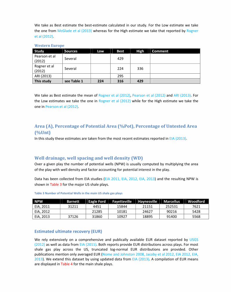
We take as Best estimate the best-estimate calculated in our study. For the Low estimate we take

the one from McGlade et al (2013) whereas for the High estimate we take that reported by Rogner

et al (2012).

Western Europe

Study Sources Low Best High Comment

Pearson et al

(2012) Several 429

Rogner et al

(2012) Several 224 336

ARI (2013) 295

This study see Table 1 224 316 429

We take as Best estimate the mean of Rogner et al (2012), Pearson et al (2012) and ARI (2013). For

the Low estimates we take the one in Rogner et al (2012) while for the High estimate we take the

one in Pearson et al (2012).

Area (A), Percentage of Potential Area (%Pot), Percentage of Untested Area

(%Unt)

In this study these estimates are taken from the most recent estimates reported in EIA (2013).

Well drainage, well spacing and well density (WD)

Over a given play the number of potential wells (NPW) is usually computed by multiplying the area

of the play with well density and factor accounting for potential interest in the play.

Data has been collected from EIA studies (EIA 2011, EIA, 2012, EIA, 2013) and the resulting NPW is

shown in Table 3 for the major US shale plays.

Table 3 Number of Potential Wells in the main US shale gas plays

NPW Barnett Eagle Ford Fayetteville Haynesville Marcellus Woodford

EIA, 2011 31211 4451 15844 21151 252531 7621

EIA, 2012 21285 10181 24627 90216 5428

EIA, 2013 37126 31860 10927 18895 91400 5568

Estimated ultimate recovery (EUR)

We rely extensively on a comprehensive and publically available EUR dataset reported by USGS

(2012) as well as data from EIA (2011). Both reports provide EUR distributions across plays. For most

shale gas play across the US, truncated log-normal EUR distributions are provided. Other

publications mention only averaged EUR (Nome and Johnston 2008, Jacoby et al 2012, EIA 2012, EIA,

2013). We extend this dataset by using updated data from EIA (2013). A compilation of EUR means

are displayed in Table 4 for the main shale plays.

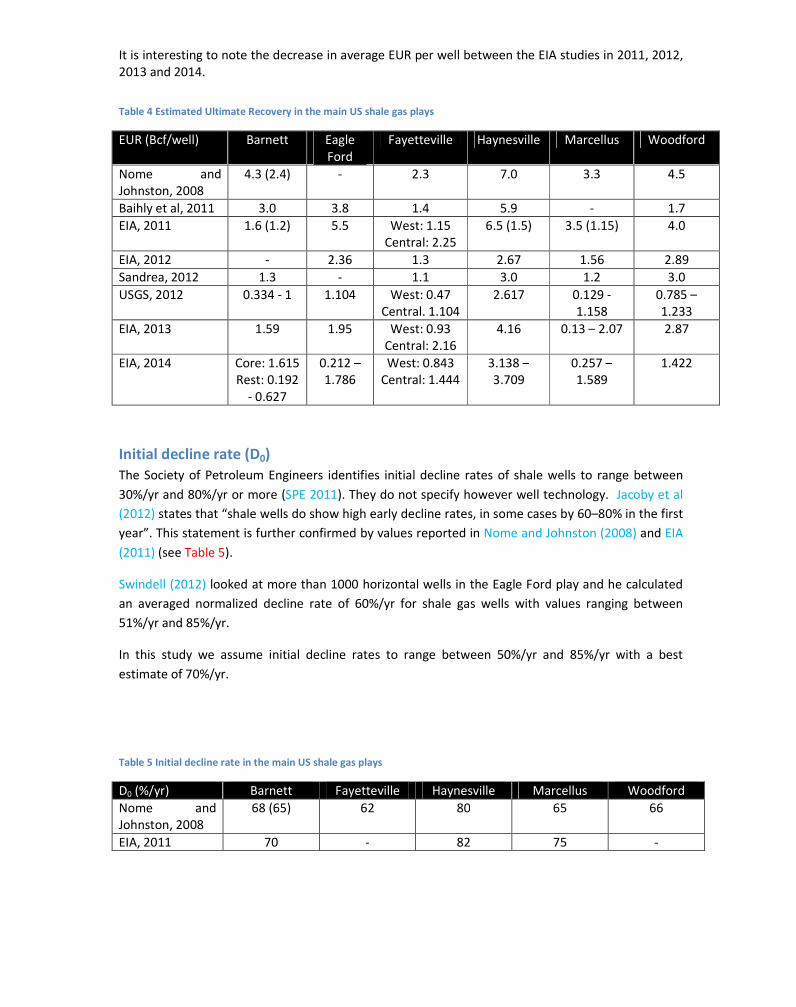
It is interesting to note the decrease in average EUR per well between the EIA studies in 2011, 2012,

2013 and 2014.

Table 4 Estimated Ultimate Recovery in the main US shale gas plays

EUR (Bcf/well) Barnett Eagle

Ford

Fayetteville Haynesville Marcellus Woodford

Nome and

Johnston, 2008

4.3 (2.4) - 2.3 7.0 3.3 4.5

Baihly et al, 2011 3.0 3.8 1.4 5.9 - 1.7

EIA, 2011 1.6 (1.2) 5.5 West: 1.15

Central: 2.25

6.5 (1.5) 3.5 (1.15) 4.0

EIA, 2012 - 2.36 1.3 2.67 1.56 2.89

Sandrea, 2012 1.3 - 1.1 3.0 1.2 3.0

USGS, 2012 0.334 - 1 1.104 West: 0.47

Central. 1.104

2.617 0.129 -

1.158

0.785 –

1.233

EIA, 2013 1.59 1.95 West: 0.93

Central: 2.16

4.16 0.13 – 2.07 2.87

EIA, 2014 Core: 1.615

Rest: 0.192

- 0.627

0.212 –

1.786

West: 0.843

Central: 1.444

3.138 –

3.709

0.257 –

1.589

1.422

Initial decline rate (D0)

The Society of Petroleum Engineers identifies initial decline rates of shale wells to range between

30%/yr and 80%/yr or more (SPE 2011). They do not specify however well technology. Jacoby et al

(2012) states that “shale wells do show high early decline rates, in some cases by 60–80% in the first

year”. This statement is further confirmed by values reported in Nome and Johnston (2008) and EIA

(2011) (see Table 5).

Swindell (2012) looked at more than 1000 horizontal wells in the Eagle Ford play and he calculated

an averaged normalized decline rate of 60%/yr for shale gas wells with values ranging between

51%/yr and 85%/yr.

In this study we assume initial decline rates to range between 50%/yr and 85%/yr with a best

estimate of 70%/yr.

Table 5 Initial decline rate in the main US shale gas plays

D0 (%/yr) Barnett Fayetteville Haynesville Marcellus Woodford

Nome and

Johnston, 2008

68 (65) 62 80 65 66

EIA, 2011 70 - 82 75 -

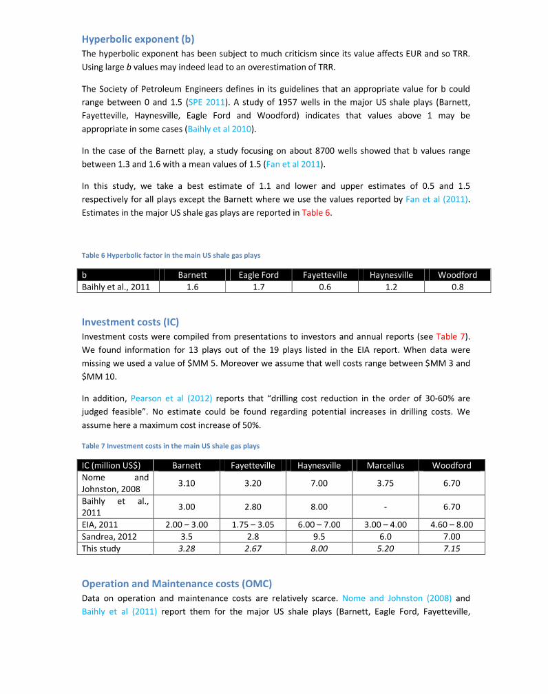
Hyperbolic exponent (b)

The hyperbolic exponent has been subject to much criticism since its value affects EUR and so TRR.

Using large b values may indeed lead to an overestimation of TRR.

The Society of Petroleum Engineers defines in its guidelines that an appropriate value for b could

range between 0 and 1.5 (SPE 2011). A study of 1957 wells in the major US shale plays (Barnett,

Fayetteville, Haynesville, Eagle Ford and Woodford) indicates that values above 1 may be

appropriate in some cases (Baihly et al 2010).

In the case of the Barnett play, a study focusing on about 8700 wells showed that b values range

between 1.3 and 1.6 with a mean values of 1.5 (Fan et al 2011).

In this study, we take a best estimate of 1.1 and lower and upper estimates of 0.5 and 1.5

respectively for all plays except the Barnett where we use the values reported by Fan et al (2011).

Estimates in the major US shale gas plays are reported in Table 6.

Table 6 Hyperbolic factor in the main US shale gas plays

b Barnett Eagle Ford Fayetteville Haynesville Woodford

Baihly et al., 2011 1.6 1.7 0.6 1.2 0.8

Investment costs (IC)

Investment costs were compiled from presentations to investors and annual reports (see Table 7).

We found information for 13 plays out of the 19 plays listed in the EIA report. When data were

missing we used a value of $MM 5. Moreover we assume that well costs range between $MM 3 and

$MM 10.

In addition, Pearson et al (2012) reports that “drilling cost reduction in the order of 30-60% are

judged feasible”. No estimate could be found regarding potential increases in drilling costs. We

assume here a maximum cost increase of 50%.

Table 7 Investment costs in the main US shale gas plays

IC (million US$) Barnett Fayetteville Haynesville Marcellus Woodford

Nome and

Johnston, 2008 3.10 3.20 7.00 3.75 6.70

Baihly et al.,

2011 3.00 2.80 8.00 - 6.70

EIA, 2011 2.00 – 3.00 1.75 – 3.05 6.00 – 7.00 3.00 – 4.00 4.60 – 8.00

Sandrea, 2012 3.5 2.8 9.5 6.0 7.00

This study 3.28 2.67 8.00 5.20 7.15

Operation and Maintenance costs (OMC)

Data on operation and maintenance costs are relatively scarce. Nome and Johnston (2008) and

Baihly et al (2011) report them for the major US shale plays (Barnett, Eagle Ford, Fayetteville,

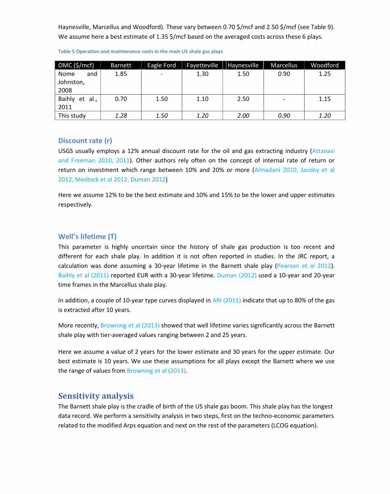
Haynesville, Marcellus and Woodford). These vary between 0.70 $/mcf and 2.50 $/mcf (see Table 9).

We assume here a best estimate of 1.35 $/mcf based on the averaged costs across these 6 plays.

Table 5 Operation and maintenance costs in the main US shale gas plays

OMC ($/mcf) Barnett Eagle Ford Fayetteville Haynesville Marcellus Woodford

Nome and

Johnston,

2008

1.85 - 1.30 1.50 0.90 1.25

Baihly et al.,

2011

0.70 1.50 1.10 2.50 - 1.15

This study 1.28 1.50 1.20 2.00 0.90 1.20

Discount rate (r)

USGS usually employs a 12% annual discount rate for the oil and gas extracting industry (Attanasi

and Freeman 2010, 2011). Other authors rely often on the concept of internal rate of return or

return on investment which range between 10% and 20% or more (Almadani 2010, Jacoby et al

2012, Medlock et al 2012, Duman 2012)

Here we assume 12% to be the best estimate and 10% and 15% to be the lower and upper estimates

respectively.

Well’s lifetime (T)

This parameter is highly uncertain since the history of shale gas production is too recent and

different for each shale play. In addition it is not often reported in studies. In the JRC report, a

calculation was done assuming a 30-year lifetime in the Barnett shale play (Pearson et al 2012).

Baihly et al (2011) reported EUR with a 30-year lifetime. Duman (2012) used a 10-year and 20-year

time frames in the Marcellus shale play.

In addition, a couple of 10-year type curves displayed in ARI (2011) indicate that up to 80% of the gas

is extracted after 10 years.

More recently, Browning et al (2013) showed that well lifetime varies significantly across the Barnett

shale play with tier-averaged values ranging between 2 and 25 years.

Here we assume a value of 2 years for the lower estimate and 30 years for the upper estimate. Our

best estimate is 10 years. We use these assumptions for all plays except the Barnett where we use

the range of values from Browning et al (2013).

Sensitivity analysis The Barnett shale play is the cradle of birth of the US shale gas boom. This shale play has the longest

data record. We perform a sensitivity analysis in two steps, first on the techno-economic parameters

related to the modified Arps equation and next on the rest of the parameters (LCOG equation).

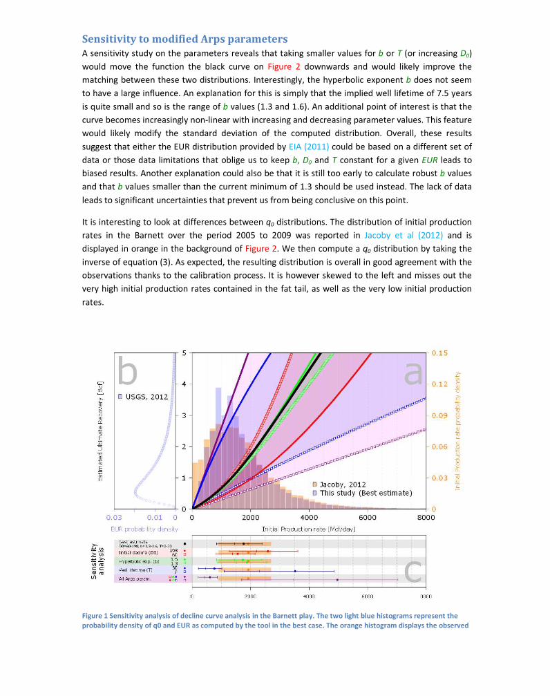
Sensitivity to modified Arps parameters

A sensitivity study on the parameters reveals that taking smaller values for b or T (or increasing D0)

would move the function the black curve on Figure 2 downwards and would likely improve the

matching between these two distributions. Interestingly, the hyperbolic exponent b does not seem

to have a large influence. An explanation for this is simply that the implied well lifetime of 7.5 years

is quite small and so is the range of b values (1.3 and 1.6). An additional point of interest is that the

curve becomes increasingly non-linear with increasing and decreasing parameter values. This feature

would likely modify the standard deviation of the computed distribution. Overall, these results

suggest that either the EUR distribution provided by EIA (2011) could be based on a different set of

data or those data limitations that oblige us to keep b, D0 and T constant for a given EUR leads to

biased results. Another explanation could also be that it is still too early to calculate robust b values

and that b values smaller than the current minimum of 1.3 should be used instead. The lack of data

leads to significant uncertainties that prevent us from being conclusive on this point.

It is interesting to look at differences between q0 distributions. The distribution of initial production

rates in the Barnett over the period 2005 to 2009 was reported in Jacoby et al (2012) and is

displayed in orange in the background of Figure 2. We then compute a q0 distribution by taking the

inverse of equation (3). As expected, the resulting distribution is overall in good agreement with the

observations thanks to the calibration process. It is however skewed to the left and misses out the

very high initial production rates contained in the fat tail, as well as the very low initial production

rates.

Figure 1 Sensitivity analysis of decline curve analysis in the Barnett play. The two light blue histograms represent the

probability density of q0 and EUR as computed by the tool in the best case. The orange histogram displays the observed

IP rates as reported by Jacoby et al (2012). The black line represents the best case whereas the dashed lines represent

the lower and upper bound of the range of values reported in the literature for D0 (red), b (green) and T (blue). The

purple curves and areas correspond to extreme cases in which all parameters were switched to their lower or upper

estimates. The black triangles on panels (a) and (b) indicate the data points provided in EIA (2011).

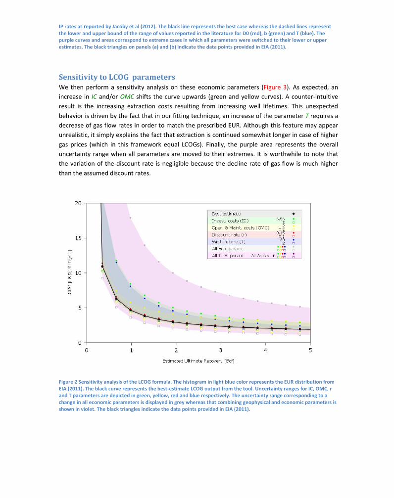
Sensitivity to LCOG parameters

We then perform a sensitivity analysis on these economic parameters (Figure 3). As expected, an

increase in IC and/or OMC shifts the curve upwards (green and yellow curves). A counter-intuitive

result is the increasing extraction costs resulting from increasing well lifetimes. This unexpected

behavior is driven by the fact that in our fitting technique, an increase of the parameter T requires a

decrease of gas flow rates in order to match the prescribed EUR. Although this feature may appear

unrealistic, it simply explains the fact that extraction is continued somewhat longer in case of higher

gas prices (which in this framework equal LCOGs). Finally, the purple area represents the overall

uncertainty range when all parameters are moved to their extremes. It is worthwhile to note that

the variation of the discount rate is negligible because the decline rate of gas flow is much higher

than the assumed discount rates.

Figure 2 Sensitivity analysis of the LCOG formula. The histogram in light blue color represents the EUR distribution from

EIA (2011). The black curve represents the best-estimate LCOG output from the tool. Uncertainty ranges for IC, OMC, r

and T parameters are depicted in green, yellow, red and blue respectively. The uncertainty range corresponding to a

change in all economic parameters is displayed in grey whereas that combining geophysical and economic parameters is

shown in violet. The black triangles indicate the data points provided in EIA (2011).

CECF regressions As mentioned in the main text we fit 3

rd-order polynomials to our CECFs in order to facilitate the

utilization of our curves. This regression takes the following form:

;<=> ? ? ?@@ ?AA

where ;<=> is the normalized TRR and C is the LCOG (see Fig. 3 in the main text).

Case ? ? ?@ ?A

Best-estimate -4.45e-1 2.88e-1 -2.20e-2 5.90e-4

Lower estimate -1.29e-1 4.32e-1 -7.87e-3 4.65e-4

Upper estimate -4.60e-1 3.58e-1 -3.12e-2 9.26e-4

Unit conversion 1 cubic feet of natural gas = 1.055 MJ (Rogner et al 2012)

1 cubic feet of natural gas = 35.31 cubic meter of gas (Rogner et al 2012)

Glossary

Model parameters and variables

Acronym Stands for… Description

b Hyperbolic factor Factor used in the modified Arps equation (2).

D0 Initial decline rate Factor used in the modified Arps equation (2).

CECF Cumulative Extraction

Cost Function

Mathematical function that relates cumulative extraction to

marginal extraction costs in a given region.

ERR Economic Recoverable

Resources

Same as TRR but account for economic factors. (in this

study we do not include the effect of tax and royalties)

EUR Estimated Ultimate

Recovery

The expected amount of resources to be produced from a

single well. Used in equation (2).

LCOG Levelized Cost Of Gas Unit cost of producing one unit of energy including all costs

over the well lifetime. Result of equation (3).

TRR Technically Recoverable

Resources

The amount of resources that can be produced over an area

(e.g. shale play) with currently existing technologies,

discarding any economic factor. Result of equation (4)

IC investment costs In this study investment costs are represented by average

well costs. Used in equation (3).

OMC Operation and

Maintenance costs

In this study operation and maintenance costs include field

operating costs and transportation costs. Used in equation

(3).

r Discount rate Used in equation (3).

A Area Shale play area. Used in equation (1).

WD Well Density Used in equation (1).

%Pot Percentage of Potential

area

Used in equation (1).

%Unt Percentage of Untested

area

Used in equation (1).

Institutions

Acronym Stands for…

EIA Energy Information Administration

USGS United States Geological Survey

IEA International Energy Agency

References Almadani H. S. A., A methodology to determine both the technically recoverable resource and the

economically recoverable resource in an unconventional gas play

Attanasi E. D. and Freeman P. A. , “Survey of Stranded Gas and Delivered Costs to Europe of Selected

Gas Resources”, SPE Economics & Management, 2011

Attanasi E. D. and Freeman P. A., “Role of Stranded Gas from Central Asia and Russia in Meeting

Europe’S Future Import Demand for Gas”, Natural Resources Research, 2012

Advanced Resources International. World shale gas resources: an initial assessment of 14 regions

outside the United States. Washington, DC: Advanced Resources International Inc; 2011

Advanced Resources International. World shale gas and shale oil resource assessment. Washington,

DC: Advanced Resources International Inc; 2013

Baihly J., Altman R., Malpani R. and Luo F., “Study Assesses Shale Decline Rates”, The American Oil &

Gas Reporter, May 2011

BGR 2012, „Abschätzung des Erdgaspotenzials aus dichten Tongesteinen (Schiefergas) in

Deutschland“, Bundesanstalt für Geowissenschaften und Rohstoffe Hannover, May 2012

Browning J., Tinker S., Ikonnikova S., Gülen G, Potter E., Fu Q., Horvath S., Patzek T., Male F., Fisher

W., Roberts F., „Barnett Shale Model 1 & 2“, Oil and Gas Journal, 2013

Duman R. J., “Economic viability of shale gas production in the Marcellus shale, indicated by

production rates costs and current natural gas prices”, thesis, University of Michigan, 2012

EIA 2011, Review of Emerging resources US shale gas and shale oil plays, a report prepared by INTEK

for the Energy Information Administration, Washington, USA

EIA 2012, Annual Energy Outlook, Energy Information Administration, Washington, USA

EIA 2013a, Annual Energy Outlook, Energy Information Administration, Washington, USA

EIA 2013b, Technically Recoverable Shale Oil and Shale Gas resources: An Assessment of 137 Shale

Formations in 41 Countries outside the United States, a report prepared by ARI for the Energy

Information Administration, Washington, USA

EIA 2014, Annual Energy Outlook, Energy Information Administration, Washington, USA

Fan L., Luo F., Lindsay G., Thompson J., Robinson J., “The Bottom-line of Horizontal Well Production

Decline in the Barnett Shale”, Conference Paper, Society of Petroleum Engineers, 2011

Jacoby H. D., O’Sullivan F. M. and Paltsev S., “The Influence of Shale Gas on U.S. Energy and

Environmental Policy”, Economics of Energy & Environmental Policy, 2012

McGlade C., Speirs J. and Sorrell S., “Unconventional gas – A review of regional and global resource

estimates”, Energy, 55, 571-584, 2013

Medlock K. B., “Modeling the implications of expanded US shale gas production”, Energy Strategy

Reviews, 2012

Nome S. and Johnston P., “From Shale to shinning shale”, Deutsche Bank Research, 2011

Pearson I. L. G., Zeniewski P., Gracceva F., Zastera P., McGlade C., Sorrell S., Speirs J., ThonHauser G.,

Aleen C., Eriksson A., Schütz M. and Toft P., “Unconventional Gas: Potential Energy market impacts

in the European Union, JRC Scientific and Policy report EU R 25305 EN, European Commission, JRC,

Institute for Energy and Transport, The Netherlands, 2012

Petak K., “Fundamental Point to Demand Growth, Stronger Prices in Long Term”, The American Oil &

Gas Reporter, October 2010

Petak K., “Impact of Natural Gas Supply on CHP Deployment”, ICF International, Spring CHP Forum, 5

May 2011

Rogner H.-H., Aguilera R. F., Archer C. L., Bertani R., Bhattacharya S., Dusseault M. B., Gagnon L.,

Haberl H., Hoogwijk M., Johnson A., Rogner M. L., Wagner H. and Yakushev V., “Energy Resources

and Potentials”, Chapter 7 in “Global Energy Assessment - Towards a Sustainable Future”, IIASA and

Cambridge University Press, 2012

SPE 2011, “Guidelines for application of the petroleum resources management system”, Society of

Petroleum Engineers (http://www.spe.org/industry/docs/PRMS_Guidelines_Nov2011.pdf)

Swindell G., “Eagle Ford Shale - An Early look at Ultimate Recovery”, SPE 158207, Society of

Petroleum Engineers, 2012

Appendix A: Investment Costs estimates The list of documents reviewed to estimate investment costs is given below.

1. EIA[2011] - ReviewOfEmergingResources.pdf

2. AnadarkoPetroleumCorp - [11-2012] - 111312APC_BOA Appendix.pdf

3. ConchoResources - [11-2012] - November Investor Presentation VFinal2.pdf (slide 14)

4. ClimarexEnergy - [11-2012] - BAML Global Energy Conf Miami.pdf

5. DevonEnergy - [2011] - DVN_2011AR_Full.pdf (own calculations from p. 14, p. 92)

6. Abraxas - [11-2012] - Presentation Stephens 11-6-12 v2.pdf

7. Baytex - [11-2012] - November Corporate Handout - Nov 15.pdf

8. Continental Resources - [11-2012] - 1pm 3Q12 Investor Presentation as of 11 9 12.pdf

9. GMX Resources - [10-2012] - Johnson+Rice+2012.pdf

10. Halcon - [10-2012] - Halcon Elephant Rollout_vFINAL6.pdf

11. Chesapeake Energy Corp. - [2012] - Annual_Report_2011.pdf

12. http://info.drillinginfo.com/urb/barnett/uncategorized/2012/07/barnett-showing-some-gray-

yet-still-providing-opportunity/

13. http://info.drillinginfo.com/urb/barnett/uncategorized/2012/02/whats-the-scoop-in-the-

barnett-combo-play/

14. EOG Resources - [2013-01] - InvPres_010713.pdf

15. XTO Energy - [2009-06] - casey_patterson.pdf

16. GMX Resources - [12-2012] - CapitalOne+Southcoast+Conference_FINAL__.pdf

17. http://info.drillinginfo.com/urb/eagleford/operators/2012/02/eog-talks-eagle-ford-ups-

reserves-discusses-best-practices/

18. http://info.drillinginfo.com/urb/eagleford/operators/2011/11/recent-ep-thoughts-cop-

newfield-hess/

19. http://info.drillinginfo.com/urb/eagleford/files/2011/10/Slide3.png

20. http://info.drillinginfo.com/urb/eagleford/operators/2011/07/a-dissection-of-the-newfield-

eagle-ford-program-seismic-science-and-rising-costs/

21. http://info.drillinginfo.com/urb/eagleford/operators/2011/07/swift-energy-finds-and-oil-sweet-

spot-increases-lateral-lengths/

22. http://info.drillinginfo.com/urb/eagleford/operators/2011/06/forest-oil-gives-insight-into-

eastern-eagle-ford-oil/

23. http://info.drillinginfo.com/urb/eagleford/operators/2011/02/rosetta-resources-details-

production-stream-breakout/

24. http://info.drillinginfo.com/urb/eagleford/operators/2010/08/quick-look-at-maverick-basin-

eagle-ford-operators-anadarko-and-newfield/

25. http://info.drillinginfo.com/urb/eagleford/operators/2010/03/geosouthern-petrohawk-and-

black-hawk-in-dewitt-county/

26. Carrizo Oil&Gas Inc. - [11-2012] - Stephens, Inc. 2012 Fall Investment Conference.pdf

27. ZaZA - [12-2012] - ZaZa Investor Presentation to Capital One Southcoast 2012 Energy

Conference.pdf

28. Halcon - [08-2012] - EnerCom_Halcon_vFINAL2.pdf

29. http://info.drillinginfo.com/urb/granitewash/operators/2011/03/forest-oil-continues-to-be-a-

top-performer-in-the-granite-wash/

30. http://info.drillinginfo.com/urb/granitewash/operators/2010/08/linn-energy-holds-2q2010-

conference-call-excited-about-tx-and-ok-granite-wash/

31. http://info.drillinginfo.com/urb/haynesville/operators/2011/08/some-operator-notes-eca-gmxr-

qep/

32. http://info.drillinginfo.com/urb/haynesville/operators/2011/03/tx-haynesville-snapshot/

33. http://info.drillinginfo.com/urb/haynesville/operators/2011/01/to-scale-back-and-to-choke-

back-that-is-the-haynesville-question/

34. http://info.drillinginfo.com/urb/haynesville/operators/2010/05/comstock-lease-positions-and-

quarterly-earnings-call/

35. GoodrichPetroleum - [11-2012] - 2012_Nov07_RaymondJames.pdf

36. AnadarkoPetroleumCorp - [11-2012] - 111312APC_BOA Appendix.pdf

37. http://info.drillinginfo.com/urb/marcellus/operators/2011/01/eqt-marcellus-assets-producing-

strong/

38. Gastar - [11-2012] - Nov_2012_Jefferies.pdf

39. http://info.drillinginfo.com/urb/niobrara/operators/2010/11/voyager-and-slawson-are-excited-

about-initial-dj-basin-discovery-wells/

40. http://info.drillinginfo.com/urb/niobrara/operators/2010/10/carrizos-niobrara-plan/

41. http://info.drillinginfo.com/urb/niobrara/operators/2010/06/eog-getting-serious-in-the-

niobrara/

42. GoodrichPetroleum - [11-2012] - 2012_Nov08_BMO.pdf

43. Altai Resources - [2010] - 10_Apr.pdf

44. Gulfport Energy - [11-2012] - DUGEast_11-14-12.pdf

45. http://info.drillinginfo.com/urb/wolfberry/operators/2011/11/approach-resources-update-

offset-el-paso-acreage-key-horizontals/

46. http://info.drillinginfo.com/urb/wolfberry/operators/2011/02/pioneer-gives-4q2010-wolfberry-

update-horizontals-and-cost-control/

47. http://info.drillinginfo.com/urb/wolfberry/operators/2010/05/petroleum-development-corp-

wants-in/

48. http://info.drillinginfo.com/urb/wolfberry/operators/2010/04/clayton-williams-ramps-up-

wolfberry-program/

49. http://info.drillinginfo.com/urb/wolfberry/operators/2010/03/upton-county-wolfberry-is-

producing-attractive-wells/

50. http://info.drillinginfo.com/urb/wolfberry/uncategorized/2010/03/concho-to-drill-300-texas-

wolfberry-locations-in-2010/

51. http://info.drillinginfo.com/urb/woodford/uncategorized/2012/05/some-recent-top-operator-

notes-in-the-woodford/

52. http://info.drillinginfo.com/urb/woodford/operators/2010/10/newfield-woodford-update/

53. http://info.drillinginfo.com/urb/woodford/operators/2010/05/continental-impressed-with-the-

cana-woodford/

54. Continental Resources - [11-2012] - 1pm 3Q12 Investor Presentation as of 11 9 12.pdf