Embed Size (px)
Citation preview
'
&
$
%
Boosted PLS Regression: Seminaire J.P. Fenelon 2008-1
Boosted Partial Least-Squares
Regression
Jean-Francois Durand
Montpellier II University, France
E-Mail: [email protected]
Web site: www.jf-durand-pls.com
'
&
$
%
Boosted PLS Regression: Seminaire J.P. Fenelon 2008-2
I. Introduction
– Machine Learning versus Data Mining
– The data mining prediction process
– Partial Least-Squares boosted by splines
II. Short introduction to splines
– Few words on smoothing splines
– Regression splines
∗ Two sets of basis functions
∗ Bivariate regression splines
∗ Least-Squares Splines
∗ Penalized Splines
III. Boosted PLS regression
– What is L2 Boosting?
– Ordinary PLS viewed as a L2 Boost algorithm
– The linear PLS regression: algorithm and model
– The building-model stage: choosing M
– PLS Splines (PLSS): a main effects additive model
∗ The PLSS model
∗ Choosing the tuning parameters
∗ Example 1: Multi-collinearity and outliers, the orange juice data
∗ Example 2: The Fisher iris data revisited by PLS boosting
– MAPLSS to capture interactions
∗ The ANOVA type model for main effects and interactions
∗ The building-model stage
∗ Example 3: Comparison between MAPLSS, MARS and BRUTO on simu-lated data
∗ Example 4: Multi-collinearity and bivariate interaction, the ”chem” data
IV. References

'
&
$
%
Boosted PLS Regression: Seminaire J.P. Fenelon 2008-3
I. Introduction
Machine Learning versus Data mining
Machine Learning: machine learning is concerned with the design
and development of algorithms and techniques that allow comput-
ers to ”learn”. The major focus of machine learning research is
to extract information from data automatically, by computational
and statistical methods. [http://www.wikipedia.org/]
Data mining: Data mining has been defined as ”the nontrivial ex-
traction of implicit, previously unknown, and potentially useful in-
formation from data” and ”the science of extracting useful informa-
tion from large data sets or databases.” [http://www.wikipedia.org/]
To be franc, I do not like very much the word ”Machine Learn-
ing”. I do prefer ”Data Mining” that suggests helping humans to
learn rather than machines... More concretely, many automatic
black-box methods involve thresholds for decision rules whose val-
ues may be more or less well understood and controlled by the lazy
user who mostly accepts the default values proposed by the author.
In the R-package, called PLSS for Partial Least-Squares Splines,
I tried to make the automatic part, inescapable to face with the
huge amount of data and computation, easy to master by on-line
conversational controls.
'
&
$
%
Boosted PLS Regression: Seminaire J.P. Fenelon 2008-4
The data mining prediction processThe timing of the data mining prediction process to be followed
with PLSS functions, can be split up into 3 steps:
1. Set up the aims of the problem and the associated schedule
conditions.
2. The building-model phase: a 2.1-2.2 round-trip until obtaining
a validated model.
2.1 Build an evolutionary training data base following the re-
tained schedule conditions.
2.2 Process the regression and validate or not the model built
on the data at hand.
3. Elaborate a scenario of prediction. A scenario allows the user
to conveniently enter new real or fictive observations to test the
validated models.
Partial Least-Squares boosted by splines
Partial Least-Squares regression [19, S. Wold et al.], in short PLS,
may be viewed as a repeated Least-Squares fit of residuals from
regressions on latent variables that are linear compromises of the
predictors and of maximum covariance with the responses. This
method is presented here in the framework of L2 boosting methods
[11, Hastie et al.], [8, J.H. Friedman], by considering PLS compo-
nents as the base learners.

'
&
$
%
Boosted PLS Regression: Seminaire J.P. Fenelon 2008-5
Historically very popular in chemistry and now in many scien-
tific domains, Partial Least-Squares regression of responses Y on
predictors X , PLS(X,Y ), produces linear models and has been re-
cently extended to ANOVA style decomposition models called PLS
Splines, PLSS, and Multivariate Additive PLS Splines, MAPLSS,
[4], [5], [12].
The key point of this nonlinear approach was inspired by the
book of A. Gifi [9] who replaced in exploratory data analysis meth-
ods, the design matrix X by the super-coding matrix B from trans-
forming the variables by B-splines. Let Bi be the coding of pre-
dictor i by B-splines, PLSS produces main effects additive models
PLSS(X,Y ) ≡ PLS(B, Y )
where B = [B1| . . . |Bp], while capturing main effects plus bivariate
interactions leads to
MAPLSS(X, Y ) ≡ PLS(B, Y )
where B = [B1| . . . |Bp ‖ . . . |Bi,i′| . . .], Bi,i′ being the tensor prod-
uct of splines for the two predictors i and i′.
The aim of this course is twofold, first to detail the theory
of that way of boosting PLS that involves regression splines in the
base learner, second to present real and simulated examples treated
by the free PLSS package available at
http://www.jf-durand-pls.com .

'
&
$
%
Boosted PLS Regression: Seminaire J.P. Fenelon 2008-6
II. Short introduction to splines
Few words on smoothing splines
Consider the signal plus noise model
yi = s(xi) + εi, i = 1 . . . n, x1 < . . . < xn ∈ [0, 1]
(ε1 . . . , εn)′ ∼ N(0, σ2In×n), σ2 is unknown and s ∈ Wm2 [0, 1]
Wm2 [0, 1] = {s/s(l) l = 1, . . . ,m− 1 are absolutely continuous, and s(m) ∈ L2[0, 1]}.
The smoothing spline estimator of s is
sλ = arg minµ∈Wm
2 [0,1]
1
n
n∑i=1
(yi − µ(xi))2 + λ
∫ 1
0
[µ(m)(t)]2dt; λ > 0
usually m = 2, to penalize convexity and overfitting.
The solution sλ is unique and belongs to the space of univariate
natural spline functions of degree 2m− 1 (usually 3) with knots
at distinct data points x1 < . . . < xn.
'
&
$
%
Boosted PLS Regression: Seminaire J.P. Fenelon 2008-7
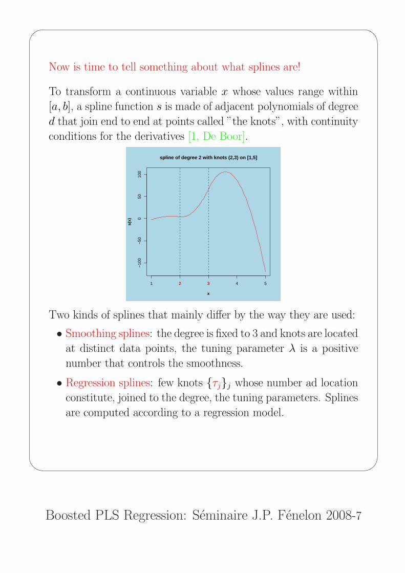
Now is time to tell something about what splines are!
To transform a continuous variable x whose values range within
[a, b], a spline function s is made of adjacent polynomials of degree
d that join end to end at points called ”the knots”, with continuity
conditions for the derivatives [1, De Boor].
1 4 5
−10
0−
500
5010
0
x
s(x)
spline of degree 2 with knots (2,3) on [1,5]
2 3
Two kinds of splines that mainly differ by the way they are used:
• Smoothing splines: the degree is fixed to 3 and knots are located
at distinct data points, the tuning parameter λ is a positive
number that controls the smoothness.
• Regression splines: few knots {τj}j whose number ad location
constitute, joined to the degree, the tuning parameters. Splines
are computed according to a regression model.

'
&
$
%
Boosted PLS Regression: Seminaire J.P. Fenelon 2008-8
Regression splines
A spline belongs to a functional linear space
S(m, {τm+1, . . . , τm+K}, [a, b])
of dimension m + K characterized by three tuning parameters
- the degree d or the order m = d + 1 of the polynomials,
- the number K and
- the location of knots {τm+1, . . . , τm+K}τ1 = . . . = τm = a < τm+1 ≤ . . . ≤ τm+K < b = τm+K+1 = . . . = τ2m+K .
A spline s ∈ S(m, {τm+1, . . . , τm+K}, [a, b]) can be written
s(x) =
m+K∑i=1
βiBmi (x)
where {Bmi (.)}i=1,...,m+K is a basis of spline functions.
The vector β of the coordinate values is to be estimated by a
regression method.

'
&
$
%
Boosted PLS Regression: Seminaire J.P. Fenelon 2008-9
Two sets of basis functions
• The truncated power functions
x −→ (x − τ )d+
1 2 3 4 5
02
46
8
x
truncated power functions at knot 2
d=1
d=3
d=2
d=0
When knots are distinct, a basis of S(m, {τm+1, . . . , τm+K}, [a, b])
is given by
1, x, . . . , xd, (x− τm+1)d+, . . . , (x− τm+K)d+
Notice that, when K = 0,
S(m, ∅, [a, b]) = the set polynomials of order m on [a, b].
'
&
$
%
Boosted PLS Regression: Seminaire J.P. Fenelon 2008-10
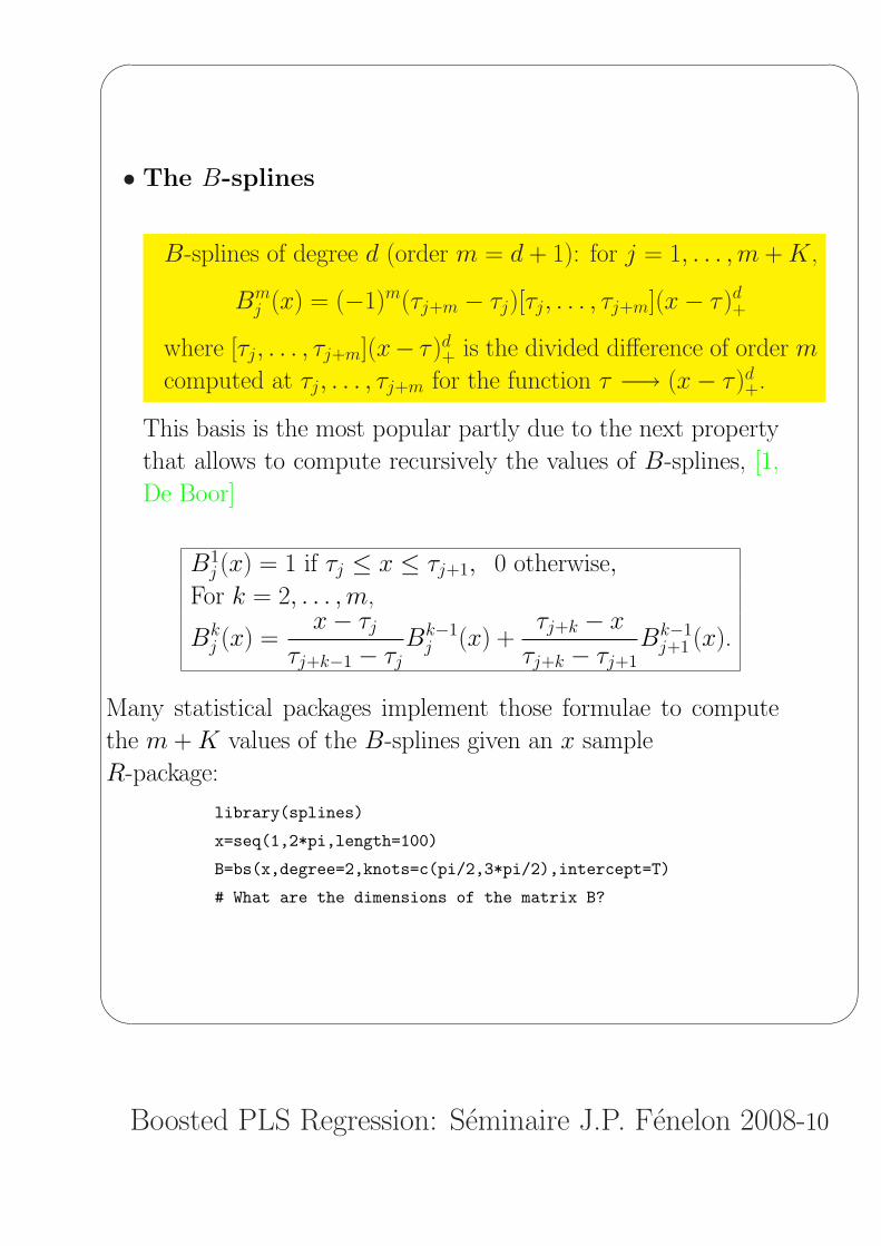
• The B-splines
B-splines of degree d (order m = d + 1): for j = 1, . . . , m + K,
Bmj (x) = (−1)m(τj+m − τj)[τj, . . . , τj+m](x− τ )d+
where [τj, . . . , τj+m](x− τ )d+ is the divided difference of order m
computed at τj, . . . , τj+m for the function τ −→ (x− τ )d+.
This basis is the most popular partly due to the next property
that allows to compute recursively the values of B-splines, [1,
De Boor]
B1j (x) = 1 if τj ≤ x ≤ τj+1, 0 otherwise,
For k = 2, . . . , m,
Bkj (x) =
x− τj
τj+k−1 − τjBk−1
j (x) +τj+k − x
τj+k − τj+1Bk−1
j+1 (x).
Many statistical packages implement those formulae to compute
the m + K values of the B-splines given an x sample
R-package:
library(splines)
x=seq(1,2*pi,length=100)
B=bs(x,degree=2,knots=c(pi/2,3*pi/2),intercept=T)
# What are the dimensions of the matrix B?
'
&
$
%
Boosted PLS Regression: Seminaire J.P. Fenelon 2008-11
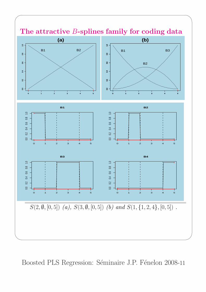
The attractive B-splines family for coding data
0 1 2 3 4 5
0.0
0.2
0.4
0.6
0.8
1.0
0 1 2 3 4 5
0.0
0.2
0.4
0.6
0.8
1.0
(a)
B1 B2
0 1 2 3 4 5
0.0
0.2
0.4
0.6
0.8
1.0
0 1 2 3 4 5
0.0
0.2
0.4
0.6
0.8
1.0
0 1 2 3 4 5
0.0
0.2
0.4
0.6
0.8
1.0
(b)
B1
B2
B3
0 1 2 3 4 5
0.00.2
0.40.6
0.81.0
B1
1
2
0 1 2 3 4 5
0.00.2
0.40.6
0.81.0
B2
1 2
0 1 2 3 4 5
0.00.2
0.40.6
0.81.0
B3
1 2
0 1 2 3 4 5
0.00.2
0.40.6
0.81.0
B4
1
2
S(2, ∅, [0, 5]) (a), S(3, ∅, [0, 5]) (b) and S(1, {1, 2, 4}, [0, 5]) .
'
&
$
%
Boosted PLS Regression: Seminaire J.P. Fenelon 2008-12
0 1 2 3 4 5
0.00.2
0.40.6
0.81.0
B1
0 1 2 3 4 5
0.00.2
0.40.6
0.81.0
B2
0 1 2 3 4 5
0.00.2
0.40.6
0.81.0
B3
0 1 2 3 4 5
0.00.2
0.40.6
0.81.0
B4
0 1 2 3 4 5
0.00.2
0.40.6
0.81.0
B5
0 1 2 3 4 5
0.00.2
0.40.6
0.81.0
B1
0 1 2 3 4 5
0.00.2
0.40.6
0.81.0
B2
0 1 2 3 4 5
0.00.2
0.40.6
0.81.0
B3
0 1 2 3 4 5
0.00.2
0.40.6
0.81.0
B4
0 1 2 3 4 5
0.00.2
0.40.6
0.81.0
B5
0 1 2 3 4 5
0.00.2
0.40.6
0.81.0
B6
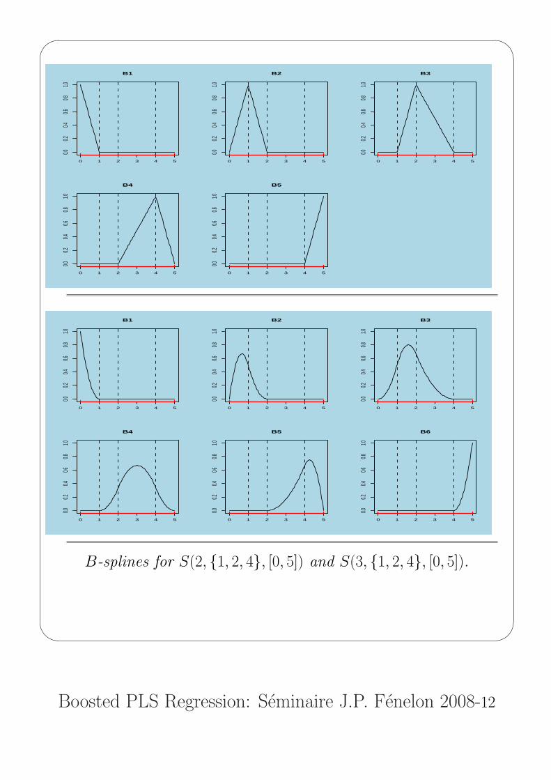
B-splines for S(2, {1, 2, 4}, [0, 5]) and S(3, {1, 2, 4}, [0, 5]).

'
&
$
%
Boosted PLS Regression: Seminaire J.P. Fenelon 2008-13
• Local support:
Bmi (x) = 0, ∀x /∈ [τi, τi+m].
♥ → One observation xi, has a local influence on s(xi) that
depends only on the m basis functions whose supports encom-
pass this data.
♠ → The counterpart is that s(x) = 0 outside [a, b].
• Fuzzy coding functions:
0 ≤ Bmi (x) ≤ 1 (1) and
m+K∑i=1
Bmi (x) = 1 (2).
♥ →Bmi (x) measures the degree of membership of x to [τi, τi+m].
The set {[τi, τi+m] |i = 1, ..., m+K} is a fuzzy partition of [a, b].
• The multiplicity of knots controls the smoothness:
The multiplicity of a knot is the number of knots that merge
at the same point. The multiplicity may vary from 1, a simple
knot, to m, a multiple knot of order m.
Let mi be the multiplicity of τi, 0 ≤ mi ≤ m,
then the first m− 1−mi right and left derivatives are equal,
s(j)− (τi) = s
(j)+ (τi), j ≤ m− 1−mi.
mi = m ⇒ discontinuity at τi
mi = 1 ⇒ locally Cm−2 at τi.

'
&
$
%
Boosted PLS Regression: Seminaire J.P. Fenelon 2008-14
• Coding a variable x through B-splines
Due to (2), two B-splines bases are generally used:
{Bmj (x) | j = 1, . . . , m + K} usual basis
{1, Bmj (x) | j = 2, . . . , m + K} , modified basis.
Let X = (x1, . . . , xn)′ be a n-sample of the variable x, denote
B = [B1(X) . . . Bm+K(X)] or B = [B2(X) . . . Bm+K(X)]
the complete n× (m + K), or incomplete n× (d + K), coding matrix
of the sample.
Notice that d = 0 provides a binary coding matrix B.
D-centering the coding matrix
When the columns of B are centered, then,
rank(B) ≤ min(n− 1, d + K).

'
&
$
%
Boosted PLS Regression: Seminaire J.P. Fenelon 2008-15
Bivariate regression splines for (x, z)
{1, Bj1(x) | j ∈ I1} and {1, Bj
2(z) | j ∈ I2} univariate bases
s(x, z) ∈ span[{1, Bj1(x)|j ∈ I1}
⊗{1, Bj2(z)|j ∈ I2}]
A bivariate regression spline split into the ANOVA decomposition:
s(x, z) = β1 +∑
j∈I1
β1j B
j1(x) +
∑
j∈I2
β2j B
j2(z) +
∑
i∈I1
∑
j∈I2
β1,2i,j Bi
1(x)Bj2(z)
main effects s1 and s2 in x and z
s1(x) =∑
j∈I1
β1j B
j1(x) s2(z) =
∑
j∈I2
β2j B
j2(z)
interaction part s12
s12(x, z) =∑
i∈I1
∑
j∈I2
β1,2i,j Bi
1(x)Bj2(z)
How to measure the importance of an ANOVA term?
by the range of the transformation (when standardized variables).
B = [B1|B2|B1,2] column centered coding matrix from X and Z.
Curse of dimensionality: expansion of the column dimension.
ncol(B1) = 10, ncol(B2) = 10, ⇒ ncol(B1,2) = 100.
'
&
$
%
Boosted PLS Regression: Seminaire J.P. Fenelon 2008-16
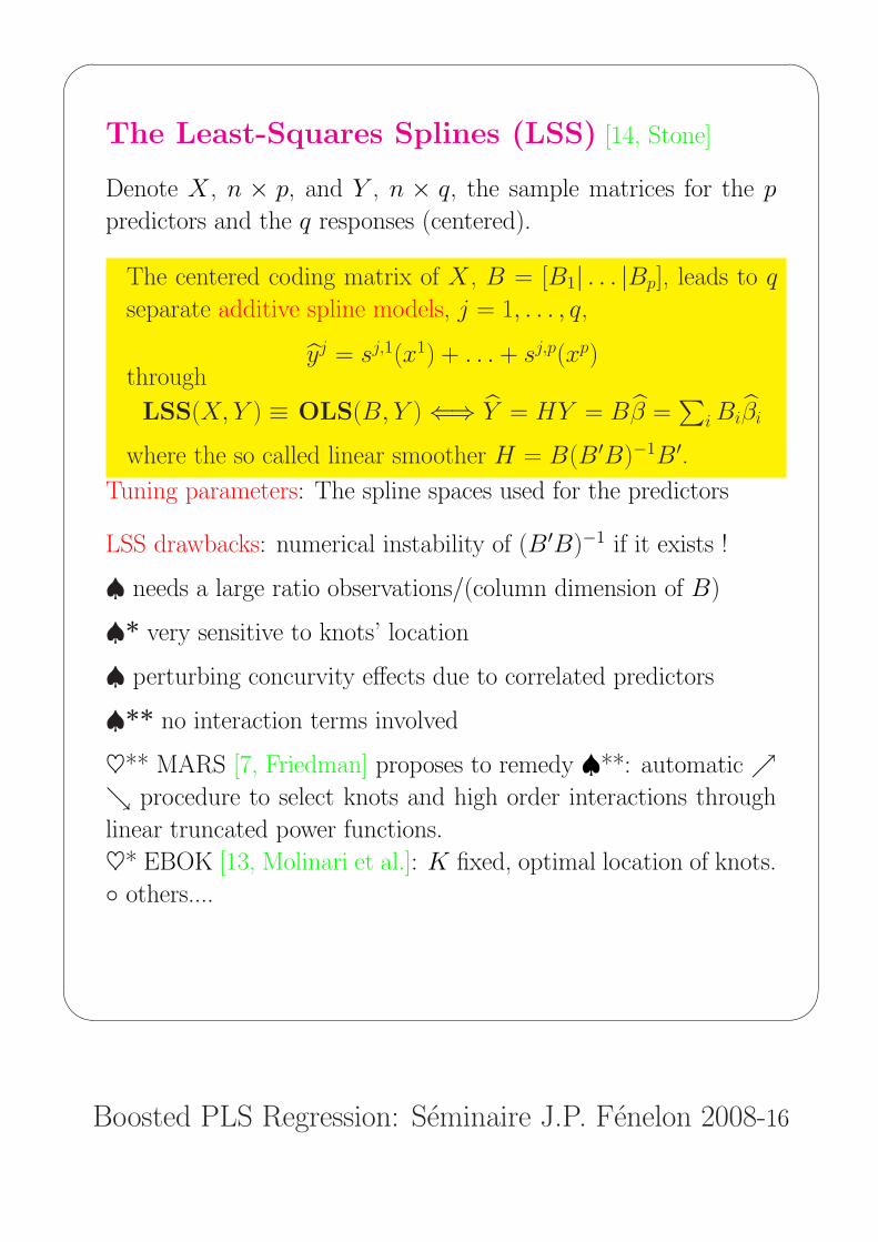
The Least-Squares Splines (LSS) [14, Stone]
Denote X , n × p, and Y , n × q, the sample matrices for the p
predictors and the q responses (centered).
The centered coding matrix of X , B = [B1| . . . |Bp], leads to q
separate additive spline models, j = 1, . . . , q,
yj = sj,1(x1) + . . . + sj,p(xp)through
LSS(X, Y ) ≡ OLS(B, Y ) ⇐⇒ Y = HY = Bβ =∑
i Biβi
where the so called linear smoother H = B(B′B)−1B′.Tuning parameters: The spline spaces used for the predictors
LSS drawbacks: numerical instability of (B′B)−1 if it exists !
♠ needs a large ratio observations/(column dimension of B)
♠* very sensitive to knots’ location
♠ perturbing concurvity effects due to correlated predictors
♠** no interaction terms involved
♥** MARS [7, Friedman] proposes to remedy ♠**: automatic ↗↘ procedure to select knots and high order interactions through
linear truncated power functions.
♥* EBOK [13, Molinari et al.]: K fixed, optimal location of knots.
◦ others....

'
&
$
%
Boosted PLS Regression: Seminaire J.P. Fenelon 2008-17
The Penalized Least-Squares Splines[6, P. Eilers and B. Marx]
Because of drawbacks cited above, L-S Splines are mostly efficient
in the one-dimensional context (p = 1).
In that univariate case, to remedy ♠* by using a large number of
equidistant knots, [6] proposed to penalize the L2 cost by a penalty
(λ) on k-finite differences of the coefficients of adjacent B-splines.
S =
n∑i=1
yi −
r∑j=1
βjBj(xi)
2
+ λr∑
j=k+1
(∆kβj)2
The linear smoother associated to the P-splines model becomes
H = B(B′B + λDk′Dk)
−1B′
Notice that λ = 0 leads to LSS and k = 0 to ridge regression.
Default : k = 2 (strong connection with second derivatives)
example : r = ncol(B) = 5 D2 =
1 −2 1 0 0
0 1 −2 1 0
0 0 1 −2 1
.
Following [10, T. Hastie and R. Tibshirani]
trace(H) = effective dimension of the smoother
'
&
$
%
Boosted PLS Regression: Seminaire J.P. Fenelon 2008-18
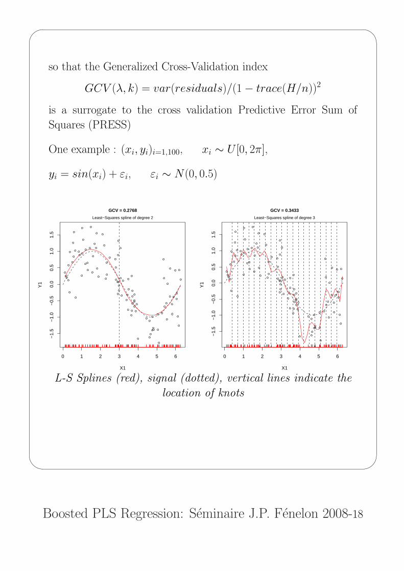
so that the Generalized Cross-Validation index
GCV (λ, k) = var(residuals)/(1− trace(H/n))2
is a surrogate to the cross validation Predictive Error Sum of
Squares (PRESS)
One example : (xi, yi)i=1,100, xi ∼ U [0, 2π],
yi = sin(xi) + εi, εi ∼ N(0, 0.5)
0 1 2 3 4 5 6
−1.
5−
1.0
−0.
50.
00.
51.
01.
5
GCV = 0.2768
X1
Y1
Least−Squares spline of degree 2
0 1 2 3 4 5 6
−1.
5−
1.0
−0.
50.
00.
51.
01.
5GCV = 0.3433
X1
Y1
Least−Squares spline of degree 3
L-S Splines (red), signal (dotted), vertical lines indicate the
location of knots
'
&
$
%
Boosted PLS Regression: Seminaire J.P. Fenelon 2008-19
0 1 2 3 4 5 6
−1.
5−
1.0
−0.
50.
00.
51.
01.
5
GCV(lambda=0.2, diff=2) = 0.2705
X1
Y1
Penalized Least−Squares spline of degree 3
0 1 2 3 4 5 6−
1.5
−1.
0−
0.5
0.0
0.5
1.0
1.5
GCV(lambda=1.5, diff=2) = 0.2969
X1
Y1
Penalized Least−Squares spline of degree 3
0 1 2 3 4 5 6
−1.
5−
1.0
−0.
50.
00.
51.
01.
5
GCV(lambda=3, diff=2) = 0.3252
X1
Y1
Penalized Least−Squares spline of degree 3
0 1 2 3 4 5 6
−1.
5−
1.0
−0.
50.
00.
51.
01.
5
GCV(lambda=30, diff=2) = 0.4267
X1
Y1
Penalized Least−Squares spline of degree 3
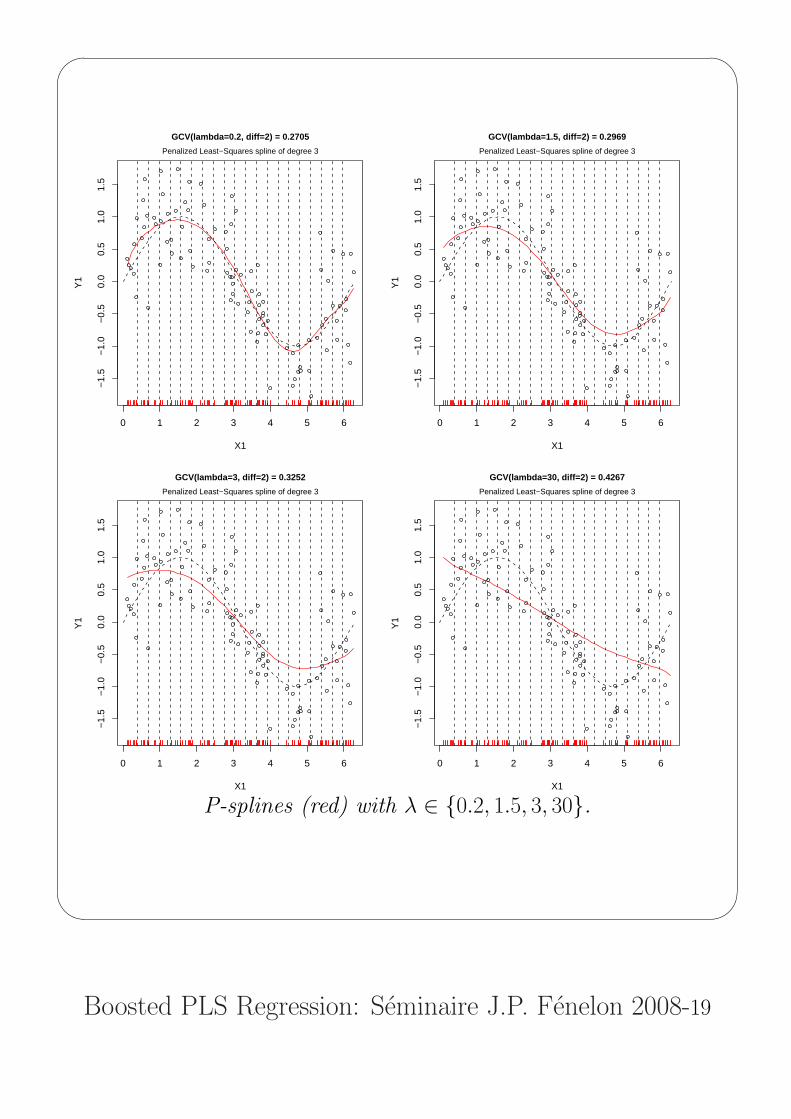
P-splines (red) with λ ∈ {0.2, 1.5, 3, 30}.
'
&
$
%
Boosted PLS Regression: Seminaire J.P. Fenelon 2008-20
III. Boosted PLS regression
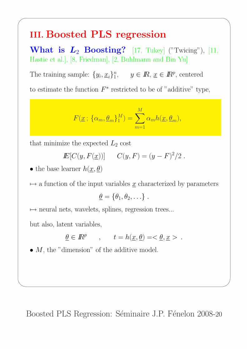
What is L2 Boosting? [17, Tukey] (”Twicing”), [11,
Hastie et al.], [8, Friedman], [2, Buhlmann and Bin Yu]
The training sample: {yi, xi}n1 , y ∈ IR, x ∈ IRp, centered
to estimate the function F ∗ restricted to be of ”additive” type,
F (x ; {αm, θm}M1 ) =
M∑m=1
αmh(x, θm),
that minimize the expected L2 cost
IE[C(y, F (x))] C(y, F ) = (y − F )2/2 .
• the base learner h(x, θ)
7→ a function of the input variables x characterized by parameters
θ = {θ1, θ2, . . .} .
7→ neural nets, wavelets, splines, regression trees...
but also, latent variables,
θ ∈ IRp , t = h(x, θ) =< θ, x > .
• M , the ”dimension” of the additive model.

'
&
$
%
Boosted PLS Regression: Seminaire J.P. Fenelon 2008-21
Boosting:
a stagewise functional gradient descent method with respect to F .
L2 boost algorithm:
F0(x) = 0
For m = 1 to M do
yi = −∂C(yi,F )∂F |F=Fm−1(xi) = yi − Fm−1(xi), i = 1, n,
(αm, θm) = arg minα,θ
n∑i=1
[yi − αh(xi; θ)]2 (∗)
Fm(x) = Fm−1(x) + αmh(x; θm)
endFor
Extended L2 boost algorithm:
Replace (∗) by
Criterion or procedure to construct θm from {(xi, yi)}i=1,n, (∗1)
αm = arg minα
n∑i=1
[yi − αh(xi; θm)]2. (∗2)
To summarize, L2 boosting is characterized by
• choosing the type of the base learner
• repeated least-squares fitting of residuals
• fitting the data by a linear combination of the base learners.
'
&
$
%
Boosted PLS Regression: Seminaire J.P. Fenelon 2008-22
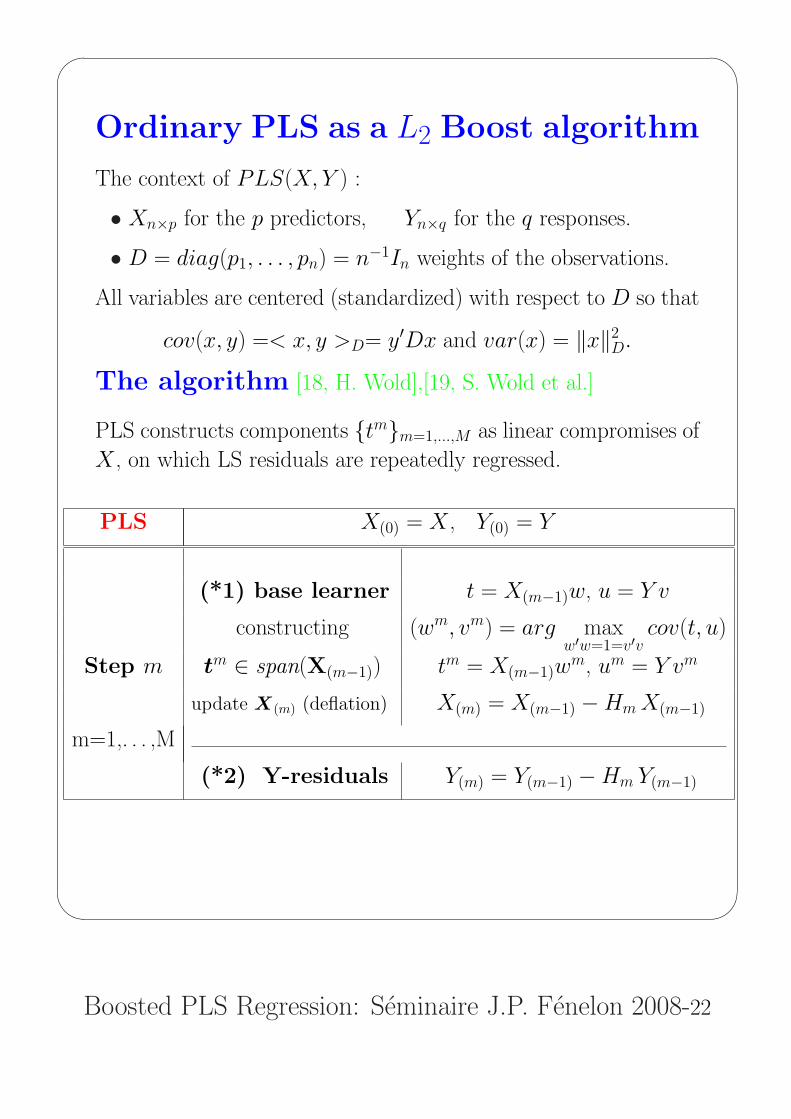
Ordinary PLS as a L2 Boost algorithm
The context of PLS(X, Y ) :
• Xn×p for the p predictors, Yn×q for the q responses.
• D = diag(p1, . . . , pn) = n−1In weights of the observations.
All variables are centered (standardized) with respect to D so that
cov(x, y) =< x, y >D= y′Dx and var(x) = ‖x‖2D.
The algorithm [18, H. Wold],[19, S. Wold et al.]
PLS constructs components {tm}m=1,...,M as linear compromises of
X , on which LS residuals are repeatedly regressed.
PLS X(0) = X , Y(0) = Y
(*1) base learner t = X(m−1)w, u = Y v
constructing (wm, vm) = arg maxw′w=1=v′v
cov(t, u)
Step m tm ∈ span(X(m−1)) tm = X(m−1)wm, um = Y vm
update X(m) (deflation) X(m) = X(m−1) −Hm X(m−1)
m=1,. . . ,M
(*2) Y-residuals Y(m) = Y(m−1) −Hm Y(m−1)

'
&
$
%
Boosted PLS Regression: Seminaire J.P. Fenelon 2008-23
where the so-called linear PLS learner,
Hm = ΠDtm = tmtm′D/‖tm‖2
D
is the n× n D-orthogonal Least-Squares projector onto tm.
Notice that the projector Hm depends also on Y since tm is of
maximum covariance with a Y -compromise .
To solve the optimization problem 1) with two constraints,
the Lagrange multipliers technique leads to
Proposition : The PLS base learner problem is solved by the
first term in the singular value decomposition of the p×q covari-
ance matrix
X ′(m−1)DY.
Let (λm, wm, vm) be the triple corresponding to the largest (first)
singular value λm, then
tm = X(m−1)wm, um = Y vm, λm = cov(tm, um).
In the one-response case, vm = 1 and wm = X ′(m−1)DY/||X ′
(m−1)DY ||.

'
&
$
%
Boosted PLS Regression: Seminaire J.P. Fenelon 2008-24
Components {tm}• belong to span(X), that is tm = Xθm
• are mutually D-orthogonal tm1 ′Dtm2 = 0, m1 6= m2 .
• Partial Regressions of pseudo variables give the same results as
LS regressions of the original variables on the components.
Xm = HmX(m−1) = HmX = tmpm′
Ym = HmY(m−1) = HmY = tmαm′
��������
��
����
��������
��
������
������
0R
n( D),
t
LS regression line
slope : ami
Y m-1( )
t
i
ami
m m
LS regressions of both responses
=
Y
Ytm ^
i
iY m
i^=
Yi
Yi
(m-1 )
mean individual
on the component t m
pseudo Yi
(m-1 ) and natural Yi
'
&
$
%
Boosted PLS Regression: Seminaire J.P. Fenelon 2008-25
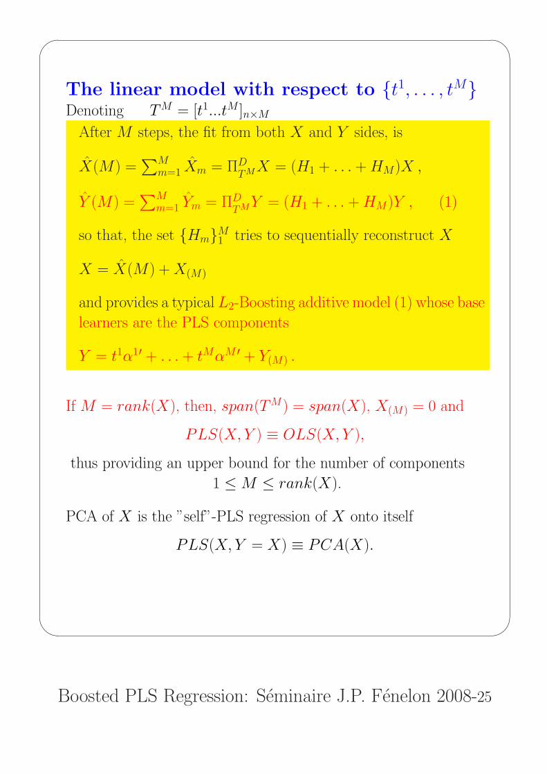
The linear model with respect to {t1, . . . , tM}Denoting TM = [t1...tM ]n×M
After M steps, the fit from both X and Y sides, is
X(M) =∑M
m=1 Xm = ΠDTMX = (H1 + . . . + HM)X ,
Y (M) =∑M
m=1 Ym = ΠDTMY = (H1 + . . . + HM)Y , (1)
so that, the set {Hm}M1 tries to sequentially reconstruct X
X = X(M) + X(M)
and provides a typical L2-Boosting additive model (1) whose base
learners are the PLS components
Y = t1α1′ + . . . + tMαM ′ + Y(M) .
If M = rank(X), then, span(TM) = span(X), X(M) = 0 and
PLS(X,Y ) ≡ OLS(X,Y ),
thus providing an upper bound for the number of components
1 ≤ M ≤ rank(X).
PCA of X is the ”self”-PLS regression of X onto itself
PLS(X, Y = X) ≡ PCA(X).
'
&
$
%
Boosted PLS Regression: Seminaire J.P. Fenelon 2008-26
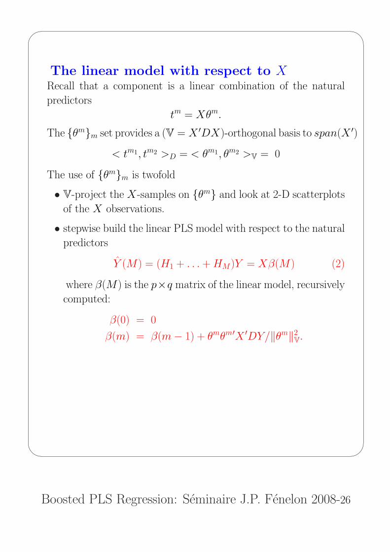
The linear model with respect to XRecall that a component is a linear combination of the natural
predictors
tm = Xθm.
The {θm}m set provides a (V = X ′DX)-orthogonal basis to span(X ′)
< tm1, tm2 >D = < θm1, θm2 >V = 0
The use of {θm}m is twofold
• V-project the X-samples on {θm} and look at 2-D scatterplots
of the X observations.
• stepwise build the linear PLS model with respect to the natural
predictors
Y (M) = (H1 + . . . + HM)Y = Xβ(M) (2)
where β(M) is the p×q matrix of the linear model, recursively
computed:
β(0) = 0
β(m) = β(m− 1) + θmθm′X ′DY/‖θm‖2V.
'
&
$
%
Boosted PLS Regression: Seminaire J.P. Fenelon 2008-27
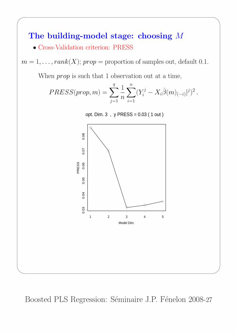
The building-model stage: choosing M
• Cross-Validation criterion: PRESS
m = 1, . . . , rank(X); prop = proportion of samples out, default 0.1.
When prop is such that 1 observation out at a time,
PRESS(prop, m) =
q∑j=1
1
n
n∑i=1
(Y ji −Xiβ(m)(−i)|j)2 .
1 2 3 4 5
Model Dim.
0.0
30.0
40.0
50.0
60.0
70.0
8
PR
ES
S
opt. Dim. 3 , y PRESS = 0.03 ( 1 out )
'
&
$
%
Boosted PLS Regression: Seminaire J.P. Fenelon 2008-28
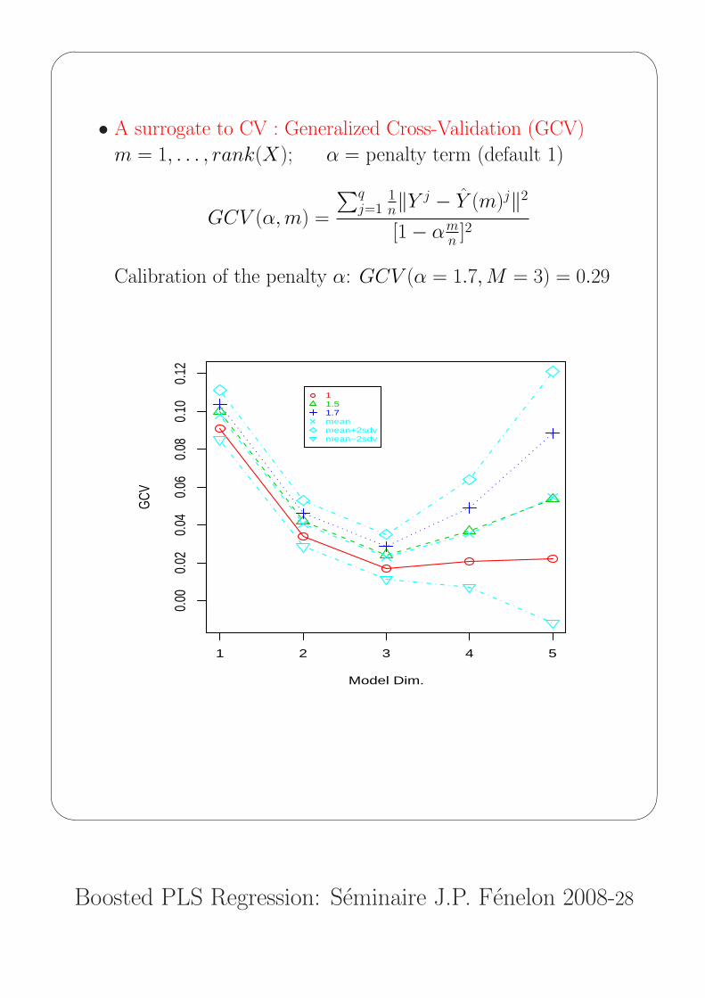
• A surrogate to CV : Generalized Cross-Validation (GCV)
m = 1, . . . , rank(X); α = penalty term (default 1)
GCV (α, m) =
∑qj=1
1n‖Y j − Y (m)j‖2
[1− αmn ]2
Calibration of the penalty α: GCV (α = 1.7,M = 3) = 0.29
Model Dim.
GCV
1 2 3 4 5
0.00
0.02
0.04
0.06
0.08
0.10
0.12
11.51.7meanmean+2sdvmean−2sdv
'
&
$
%
Boosted PLS Regression: Seminaire J.P. Fenelon 2008-29
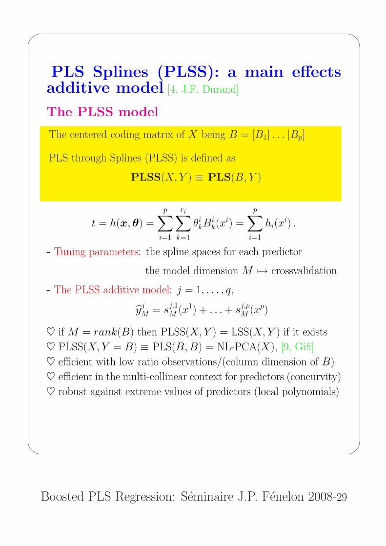
PLS Splines (PLSS): a main effectsadditive model [4, J.F. Durand]
The PLSS model
The centered coding matrix of X being B = [B1| . . . |Bp]
PLS through Splines (PLSS) is defined as
PLSS(X,Y ) ≡ PLS(B, Y )
t = h(x, θ) =
p∑i=1
ri∑
k=1
θikB
ik(x
i) =
p∑i=1
hi(xi) .
- Tuning parameters: the spline spaces for each predictor
the model dimension M 7→ crossvalidation
- The PLSS additive model: j = 1, . . . , q,
yjM = sj,1
M (x1) + . . . + sj,pM (xp)
♥ if M = rank(B) then PLSS(X, Y ) = LSS(X, Y ) if it exists
♥ PLSS(X,Y = B) ≡ PLS(B, B) = NL-PCA(X), [9, Gifi]
♥ efficient with low ratio observations/(column dimension of B)
♥ efficient in the multi-collinear context for predictors (concurvity)
♥ robust against extreme values of predictors (local polynomials)

'
&
$
%
Boosted PLS Regression: Seminaire J.P. Fenelon 2008-30
♠ ♥ no automatic procedure for choosing spline parameters
♠ no interaction terms involved
Choosing the tuning parameters
1. For each predictor: degree, number and location of knots
2. the number of PLS components 7→ cross validation
1. Two strategies for choosing the spline spaces
• The ascending strategy
– First, take d = 1 with no knots (K = 0) 7→ linear model.
– Increase the degree d, keeping K = 0, 7→ polynomial model.
– for fixed d, add knots, 7→ local polynomial model
”adding a knot increases the local flexibility of the spline
and then, the freedom of fitting the data in this area.”
• The descending strategy
– First, take a high degree, d = 3, and more knots than nec-
essary.
– Remove superfluous knots and decrease the degree as much
as possible
2. To stop a strategy : find a balance between
thriftiness (M and the total spline dimension) andgoodness-of-prediction, PRESS and/or GCV .
'
&
$
%
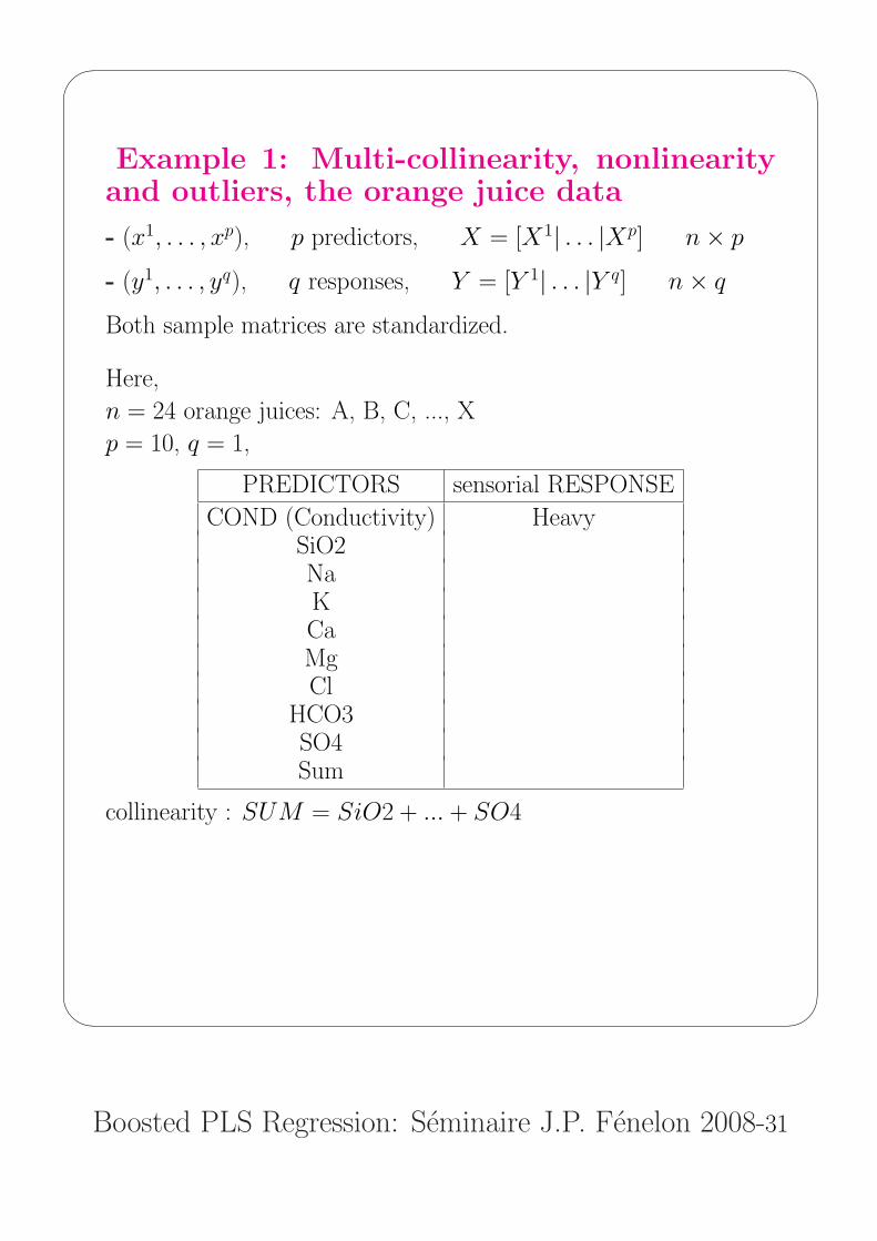
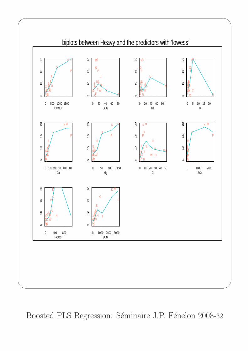
Boosted PLS Regression: Seminaire J.P. Fenelon 2008-31
Example 1: Multi-collinearity, nonlinearityand outliers, the orange juice data
- (x1, . . . , xp), p predictors, X = [X1| . . . |Xp] n× p
- (y1, . . . , yq), q responses, Y = [Y 1| . . . |Y q] n× q
Both sample matrices are standardized.
Here,
n = 24 orange juices: A, B, C, ..., X
p = 10, q = 1,
PREDICTORS sensorial RESPONSE
COND (Conductivity) HeavySiO2NaKCaMgCl
HCO3SO4Sum
collinearity : SUM = SiO2 + ... + SO4
'
&
$
%
Boosted PLS Regression: Seminaire J.P. Fenelon 2008-32
0 500 1000 1500COND
510
15
20
AB
CD
E
F
GHIJ
K
L
M
N
OP
QR
S
TU
V WX
0 20 40 60 80SiO2
510
15
20
AB
CD
E
F
GH IJ
K
L
M
N
OP
Q R
S
TU
V WX
0 20 40 60 80Na
510
15
20
AB
CD
E
F
GHIJ
K
L
M
N
OP
Q R
S
TU
V WX
0 5 10 15 20K
510
15
20
AB
CD
E
F
GHIJ
K
L
M
N
OP
Q R
S
TU
VWX
0 100 200 300 400 500Ca
510
15
20
AB
CD
E
F
GHIJ
K
L
M
N
OP
QR
S
TU
VWX
0 50 100 150Mg
510
15
20
AB
CD
E
F
GHIJ
K
L
M
N
OP
QR
S
TU
V WX
0 10 20 30 40 50Cl
510
15
20
AB
C D
E
F
G HIJ
K
L
M
N
OP
Q R
S
TU
V WX
0 1000 2000SO4
510
15
20
AB
CD
E
F
GHIJ
K
L
M
N
OP
QR
S
TU
VWX
0 400 800HCO3
510
15
20
AB
CD
E
F
G H IJ
K
L
M
N
OP
QR
S
TU
V WX
0 1000 2000 3000SUM
510
15
20
AB
CD
E
F
G H IJ
K
L
M
N
OP
QR
S
TU
V WX
biplots between Heavy and the predictors with ’lowess’
'
&
$
%
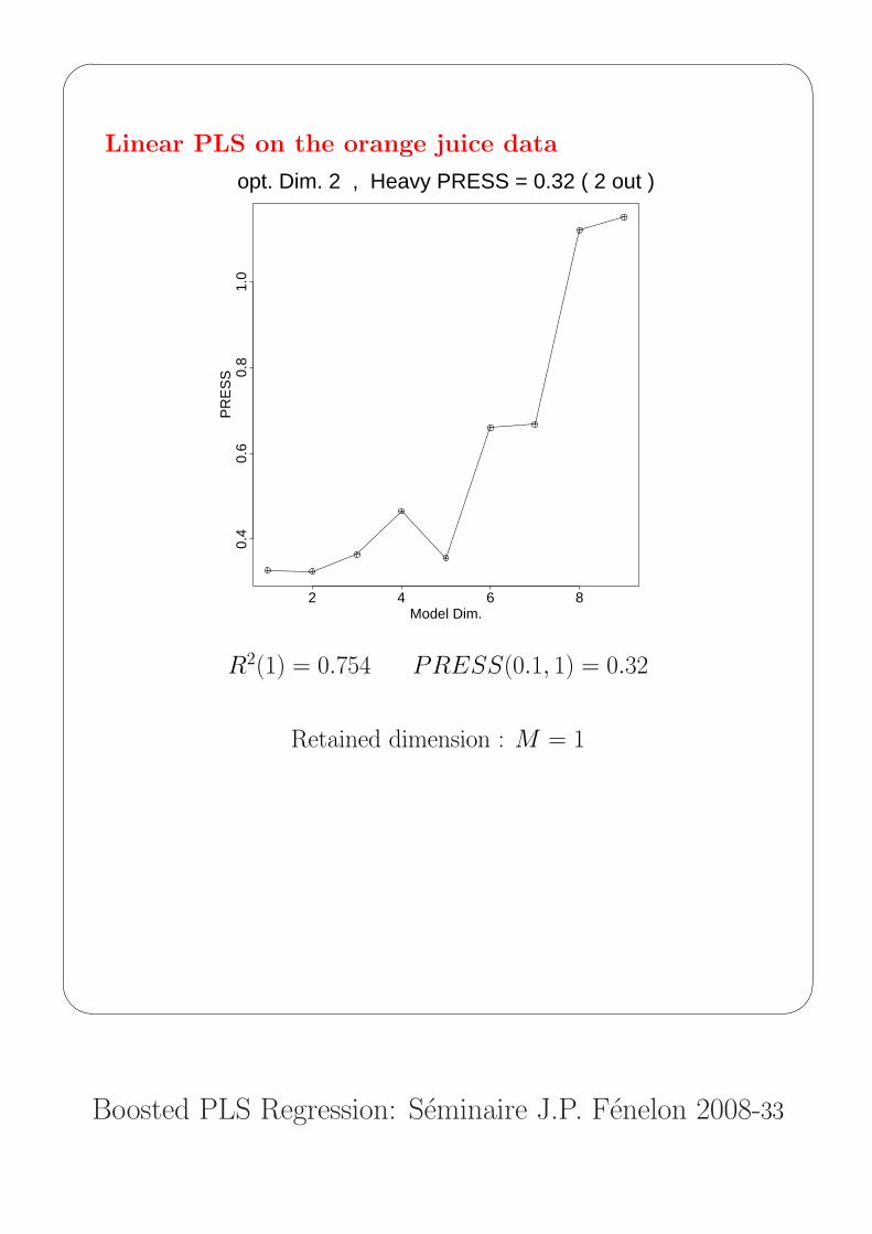
Boosted PLS Regression: Seminaire J.P. Fenelon 2008-33
Linear PLS on the orange juice data
opt. Dim. 2 , Heavy PRESS = 0.32 ( 2 out )
Model Dim.
PR
ES
S
2 4 6 8
0.4
0.6
0.8
1.0
R2(1) = 0.754 PRESS(0.1, 1) = 0.32
Retained dimension : M = 1
'
&
$
%
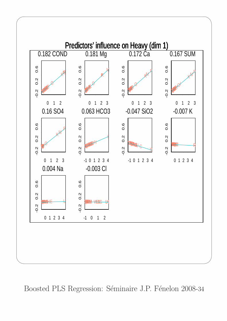
Boosted PLS Regression: Seminaire J.P. Fenelon 2008-34
0 1 2
-0.2
0.2
0.6
0.182 COND
ABCDE
FGHIJ
K
L
M
NO
P
QRSTU
VW
X
Predictors’ influence on Heavy (dim 1)
0 1 2 3
-0.2
0.2
0.6
0.181 Mg
ABCD
EFGHIJ
K
L
M
NO
P
QRSTUVWX
Predictors’ influence on Heavy (dim 1)
0 1 2 3
-0.2
0.2
0.6
0.172 Ca
ABCDEFGHIJ
K
L
M
NO
P
QRSTUVWX
Predictors’ influence on Heavy (dim 1)
0 1 2 3
-0.2
0.2
0.6
0.167 SUM
ABCD EFGH
IJ
K
L
M
NO
P
QRSTUVWX
Predictors’ influence on Heavy (dim 1)
0 1 2 3
-0.2
0.2
0.6
0.16 SO4
ABCDEFGHIJ
K
L
M
N O
P
QRSTUVWX
Predictors’ influence on Heavy (dim 1)
-1 0 1 2 3 4
-0.2
0.2
0.6
0.063 HCO3
ABCD EFGH
I
J KLMN OPQRSTUV WX
Predictors’ influence on Heavy (dim 1)
-1 0 1 2 3 4
-0.2
0.2
0.6
-0.047 SiO2
AB CD EF GH IJKLMNOPQ
RS T UV WX
Predictors’ influence on Heavy (dim 1)
0 1 2 3 4-0
.20
.20
.6
-0.007 K
AB CD EFGHIJKL MNOPQ RSTUVWX
Predictors’ influence on Heavy (dim 1)
0 1 2 3 4
-0.2
0.2
0.6
0.004 Na
ABCD EF GHIJKLMNOPQRST UV WX
Predictors’ influence on Heavy (dim 1)
-1 0 1 2
-0.2
0.2
0.6
-0.003 Cl
ABC DEF G HIJKL MNOPQ RST UV WX
Predictors’ influence on Heavy (dim 1)

'
&
$
%
Boosted PLS Regression: Seminaire J.P. Fenelon 2008-35
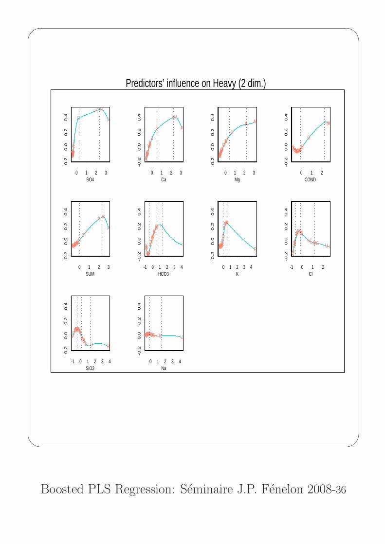
PLSS on the orange juice data
degree=2 for all predictors
Table of selected knots for the predictorsCOND SiO2 Na K Ca Mg Cl SO4 HCO3 Sum
400 10 10 2.5 160 40 4 400 100 600
1600 20 40 5 400 110 11 1700 300 2600
40 30 500
opt. Dim. 2 , Heavy PRESS = 0.154 ( 2 out )
Model Dim.
PR
ES
S
2 4 6 8 10
0.2
0.3
0.4
0.5
R2(2) = 0.917 PRESS(0.1, 2) = 0.154
'
&
$
%
Boosted PLS Regression: Seminaire J.P. Fenelon 2008-36
0 1 2 3SO4
-0.2
0.0
0.2
0.4
AB
C
D
E
FGHIJ
K
L
M
N
O P
QRST
U
VWX
0 1 2 3Ca
-0.2
0.0
0.2
0.4
A
B
CD
E
FGHIJ
K
L
M
N
O P
QR
STU
V
W
X
0 1 2 3Mg
-0.2
0.0
0.2
0.4
A
BCD
E
FGHIJ
K
L
M
N
O
P
QRS
T
UV
W
X
0 1 2COND
-0.2
0.0
0.2
0.4
ABCDEF
GHIJ
K
L
M
N
O
P
QRSTUV
WX
0 1 2 3SUM
-0.2
0.0
0.2
0.4
ABCDE
FGH
I
J
K
L
M
N
OP
QRSTU
V WX
-1 0 1 2 3 4HCO3
-0.2
0.0
0.2
0.4
AB
CD
E
FG
H
I
J
KLM
N
OP
QR
STU
V
W
X
0 1 2 3 4K
-0.2
0.0
0.2
0.4
AB
C
D
E
FGHIJ
K
L
M
N
O
P
Q
RSTU
VWX
-1 0 1 2Cl
-0.2
0.0
0.2
0.4
A
B
CDEF G
H
IJK
L
M
N
OP
Q
RS
T UV
WX
-1 0 1 2 3 4SiO2
-0.2
0.0
0.2
0.4
AB
C
DE
F
G
H
IJ
KL
MNOPQ
R
S T
U
V WX
0 1 2 3 4Na
-0.2
0.0
0.2
0.4
ABCD EF GHIJKL MNOPQ RST UV WX
Predictors’ influence on Heavy (2 dim.)
'
&
$
%
Boosted PLS Regression: Seminaire J.P. Fenelon 2008-37
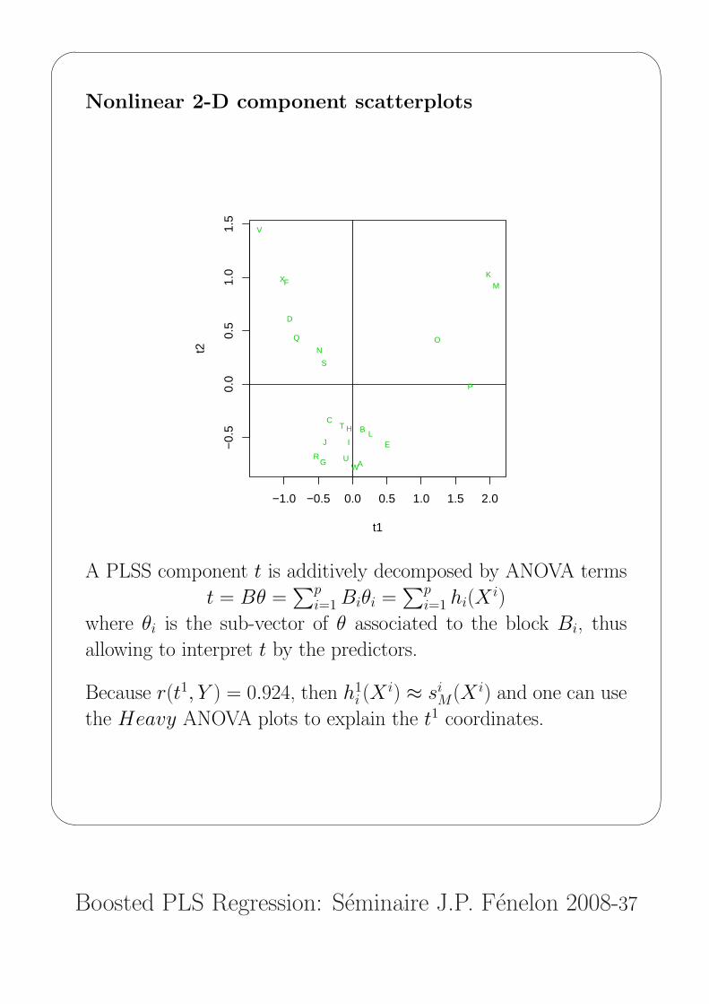
Nonlinear 2-D component scatterplots
−1.0 −0.5 0.0 0.5 1.0 1.5 2.0
−0.
50.
00.
51.
01.
5
t1
t2
A
BC
D
E
F
G
H
IJ
K
L
M
NO
P
Q
R
S
T
U
V
W
X
A PLSS component t is additively decomposed by ANOVA terms
t = Bθ =∑p
i=1 Biθi =∑p
i=1 hi(Xi)
where θi is the sub-vector of θ associated to the block Bi, thus
allowing to interpret t by the predictors.
Because r(t1, Y ) = 0.924, then h1i (X
i) ≈ siM(X i) and one can use
the Heavy ANOVA plots to explain the t1 coordinates.

'
&
$
%
Boosted PLS Regression: Seminaire J.P. Fenelon 2008-38
Example 2: The Fisher iris data revisited byPLS boosting
A multi-response PLS discriminant Analysis context, [15, Sjostrom
et al.], [16, Tenenhaus] :
p = 4 predictors: sepal width and length, petal width and length
q = 3 responses: the binary indicators of 3 Iris species,
setosa (s), versicolor (c), virginica (v)
n = 150 Iris specimen (50 per species).
The (t1, t2) scatterplot and the table of PLS diagnostics:
−3 −2 −1 0 1 2 3
−2
−1
01
2
s
s
ss
s
s
ss
s
s
s
s
ss
s
s
s
s
ss
s
s
s
s s
s
sss
ss
s
s
s
ss
s s
s
ss
s
s
s
s
s
s
s
s
s
ccc
c
c
c
c
c
c
c
c
c
c
cc
c
c
c
c
c
c
c
c
c
c
c
c
c
c
c
cc
cc
c
c
c
c
c
cc
c
c
c
c
cc
c
c
c
v
v
v
v
v
v
v
v
v
v
v
v
v
v
v
v
v
v
v
v
v
v
v
v
vv
v
vv
v
v
v
vv
v
v
v
v
v
vv v
v
vv
v
v
v
v
v
Linear PLS
Table of diagnostics
s true c true v true
s predicted 49 0 0
c predited 1 42 13
v predicted 0 8 37
PRESS(3) = 1.379, 10% out.
'
&
$
%
Boosted PLS Regression: Seminaire J.P. Fenelon 2008-39
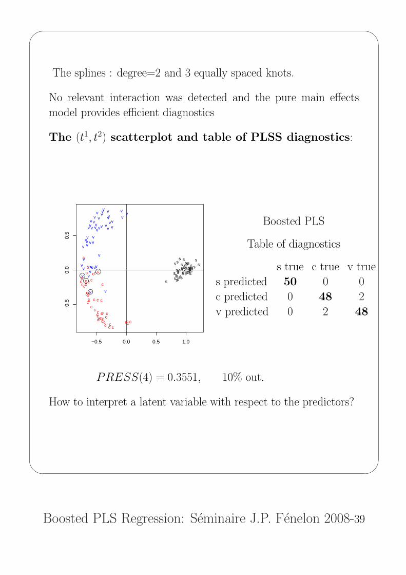
The splines : degree=2 and 3 equally spaced knots.
No relevant interaction was detected and the pure main effects
model provides efficient diagnostics
The (t1, t2) scatterplot and table of PLSS diagnostics:
−0.5 0.0 0.5 1.0
−0.
50.
00.
5
ssss s
s
ss
sss
ss
s
s
ss
ss
ss s
s
s
ss s ss
ss
ss
s
s ss
ss
sss
s
s s
s s
s
ss
cc
c
c
c
c
c
c
c
c
c
c
c
c
c
c
c
c
c
c
c
c
c
cc
cc
c
c
cc c
c
c
c
c
c
c
c
cc
c
cc
c cc
c
c
c
v
v
v
v
v v
v
v
v
v
v
v
v
v
v
v
v
v
v
v
v
v
v
v
v
v
v v
v
v
v
v
v
v v
v
v
v
v
vv
v
v
v
v
v
v
v
v
v
Boosted PLS
Table of diagnostics
s true c true v true
s predicted 50 0 0
c predicted 0 48 2
v predicted 0 2 48
PRESS(4) = 0.3551, 10% out.
How to interpret a latent variable with respect to the predictors?
'
&
$
%
Boosted PLS Regression: Seminaire J.P. Fenelon 2008-40
−1.5 0.0 1.0
−0
.20
.10
.3
Petal.Width
11111
11
11111
111
11111
1
1
1
1
11
1
1111
1
11111
11111
1
1
11
1111
2222 222
2
22
2
2
2
2222
2
2
2
22 22222 22
22
22
222222222
22
22222
2
3
33
333
333
3
3333
33
333
3
333
33
3333
3 333
33
33
333
33
3
33
3
333
3
−1.5 0.0 1.0
−0
.20
.10
.3
Petal.Length
11111111111111111111111
1111111111111111111111
11111
2222
222
2
22
2
222
2
222
22
22
2222222
2222
2222222222
2
2222
2
23
33
33
3
3
333
3333333
33
33
3
3
333
3333
33
33
33
333 3333
3333333
−2 0 1 2
−0
.20
.10
.3
Sepal.Length
1111 1
1
1 11
1
1
111
111
1
1
11
11 1111
1111
11
1
11
1
11 1111
111
111
1
22 2
2
2
2
2
2
2
22
222
2
2
22
2
22
22
22222
22
222
2
2
2
22
222
22
2
222
2
2
2
3
3
333
3
3
33
333 3
33
33
333
3
33
3 3333 333
3
333
3
333
333
3
333333
3
−2 0 1 2 3
−0
.20
.10
.3
Sepal.Width
1
1
11
1 111
11
11
11
11
11 111
1111
1
111
11
1 11
11
11
1
11
1
1
1 1
1
1
1
11
222
2 22
2
2 22
222
222
22
22
2
22 2222
22222 222
2
22 2
222
22
22222 2
3
33333
3 33
3
3
33
3 3
3
3
3
33
3
333
33
33
33
3
3
3333
3
33333
3
33
33
3
3
3
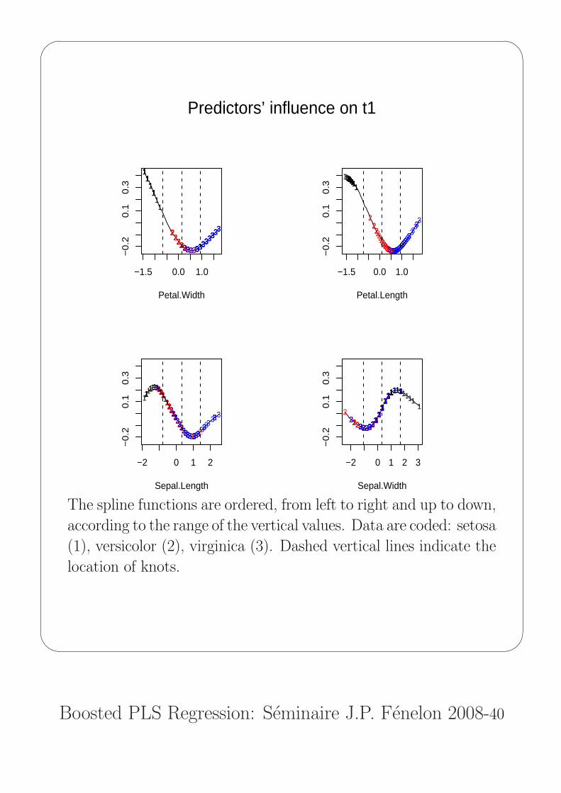
Predictors’ influence on t1
The spline functions are ordered, from left to right and up to down,
according to the range of the vertical values. Data are coded: setosa
(1), versicolor (2), virginica (3). Dashed vertical lines indicate the
location of knots.
'
&
$
%
Boosted PLS Regression: Seminaire J.P. Fenelon 2008-41
−1.5 0.0 1.0
−0
.30
.00
.2
Petal.Width
1111111111111111111111
1
1
111
11111
11111111111
1
111111
222
2
2
2
2
222
2
2
2
2222
2
2
2
2
2
2
2222
2
2
222 2
222
2
22222
222222
22
33
3
3
33
333
333
33
33
3
33
3
333
3
3
333
3
3
33
3
33
33
33
3 33
3
33
3
33
3
3
−1.5 0.0 1.0
−0
.30
.00
.2
Petal.Length
11111111111111111111111
111111111111111111111111111
22
2
2
222
2
2
2222
2
222
22
2
2
2
22
2222
2
2222
2
222
22222
2222222 2
3
3
333 3
3
333
333
3333
33
3
3
3
3
3
33
33
3333
3
3
33
33
3
33
33
33
3333
3
−2 0 1 2
−0
.30
.00
.2
Sepal.Length
11
111
1
11
1
11
11
1
1111 11
11
1
11
1111
11
11 111
11
1
11
11
111
1
1
11
2
22
2
2
2
2
2
2
22 22
2
2
2
22
2
22
22
2
2222
22222
2
2
2
2
2
222
2
22222
2
2 2
3
3
3
33
3
3
33 333
3
33
3333
3
3
3
3
3
3 3
33
3
333
333
3
33
3
333
3
333
33
3
3
−2 0 1 2 3
−0
.30
.00
.2
Sepal.Width
11 11
1 1111 1 1111 1
111 111 1111
1111111
1111 111
11
1
1 1 11
11 11222
222
2
22
222
222 22
22 2
22
22222
2222222
22
2
2
2
222
222
2222
23
33333
33
3
333
3
33
333
33
3333
333
33
33
333
33
333333
333
3
3
33
3
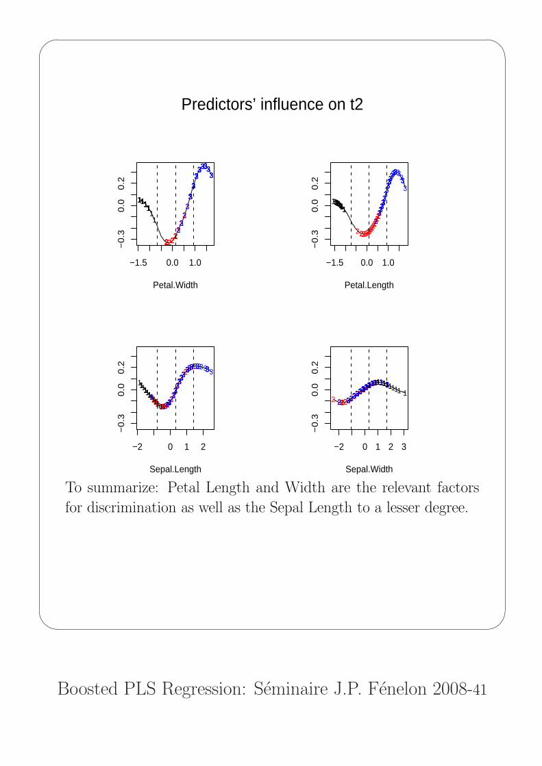
Predictors’ influence on t2
To summarize: Petal Length and Width are the relevant factors
for discrimination as well as the Sepal Length to a lesser degree.

'
&
$
%
Boosted PLS Regression: Seminaire J.P. Fenelon 2008-42
Multivariate Additive PLS Splines(MAPLSS): capture of interactions[5, Durand & Lombardo][12, Lombardo, Durand, De Veaux ]
The ANOVA type model for main effects andinteractions
The centered main effects + interactions coding matrix:
B = [B1| . . . |Bp ‖ . . . |Bi,i′| . . .]where (i, i′) belong to the set I of accepted couples of interactions
MAPLSS(X,Y ) ≡ PLS(B, Y )
t = h(x, θ) =
p∑i=1
ri∑
k=1
θikB
ik(x
i)+∑
{i,i′}∈I
[ri∑
k=1
ri′∑
l=1
θi,i′k,lB
ik(x
i)Bi′l (xi′)
].
q simultaneous models casted in the ANOVA decomposition
j = 1, . . . , q, yjM =
p∑i=1
sj,iM(xi) +
∑
(i,i′)∈Isj,ii′M (xi, xi′)
PLSS with interactions shares the preceding ♥ properties
♠ ♥ no automatic procedure for choosing spline parameters

'
&
$
%
Boosted PLS Regression: Seminaire J.P. Fenelon 2008-43
The building-model stageInputs: threshold = 20%, Mmax = dim. maximum to explore
0 Preliminary phase: the main effects model (mandatory).
Decide on the spline parameters as well as on Mm for the main
effects model (m): denote GCVm(Mm) and R2m(Mm).
1 Individual evaluation of all interactions.
Each interaction i is separately added to the main effects.
crit(Mi) = maxM∈{1,Mmax}
R2m+i(M)−R2
m(Mm)
R2m(Mm)
+GCVm(Mm)−GCVm+i(M)
GCVm(Mm)
Eliminate interactions i such that CRIT (Mi) < 0
Order decreasingly the accepted candidate interactions.
2 Add successively interactions to main effects (forward phase).
Set GCV0 = GCVm(Mm) and i = 0.
REPEAT
2 i ← i + 1
2 add interaction i and index the new model with i
2 GCVi ← optimal GCV among all dimensions
UNTIL (GCVi < GCVi−1 − threshold ∗GCVi−1)
3 prune ANOVA terms of lowest influence (backward phase)
criterion: the range of the values of the ANOVA function

'
&
$
%
Boosted PLS Regression: Seminaire J.P. Fenelon 2008-44
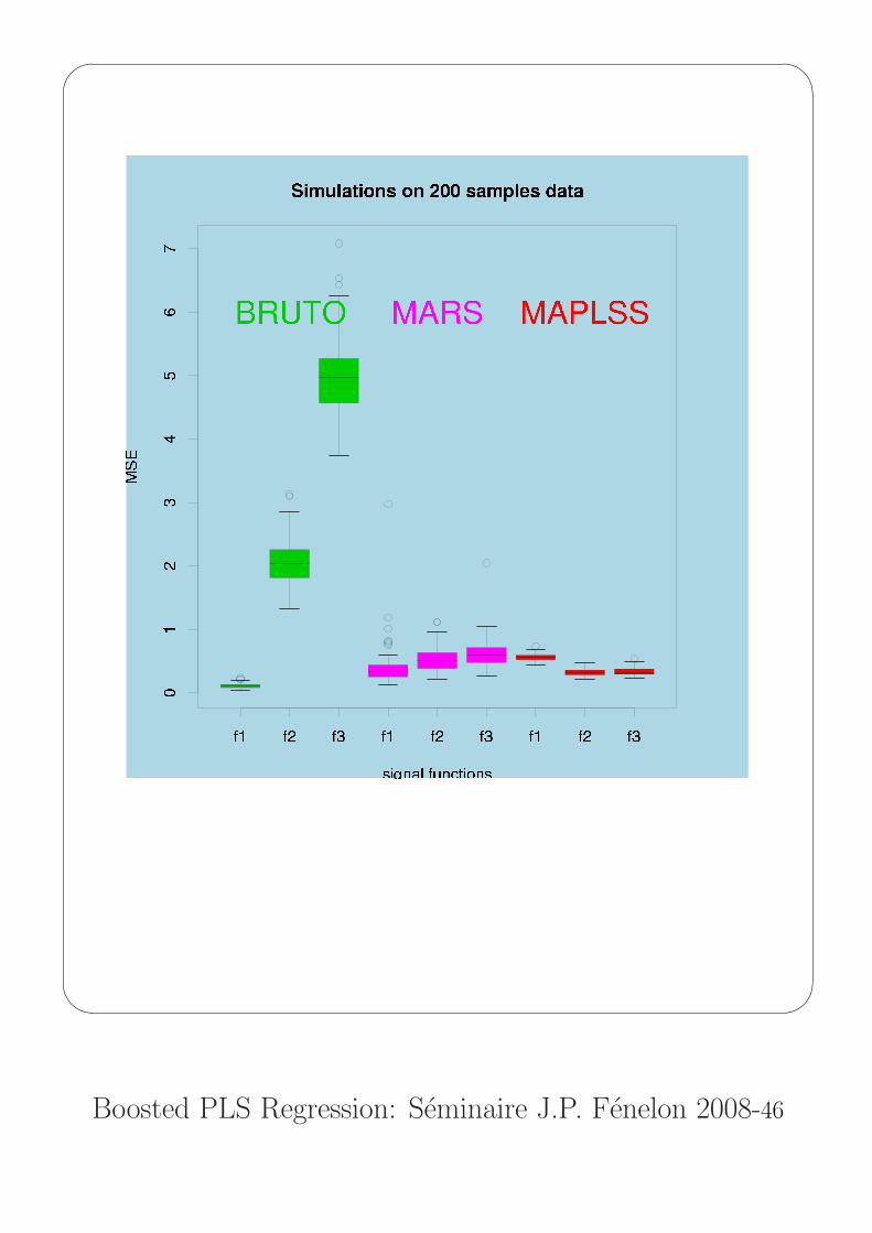
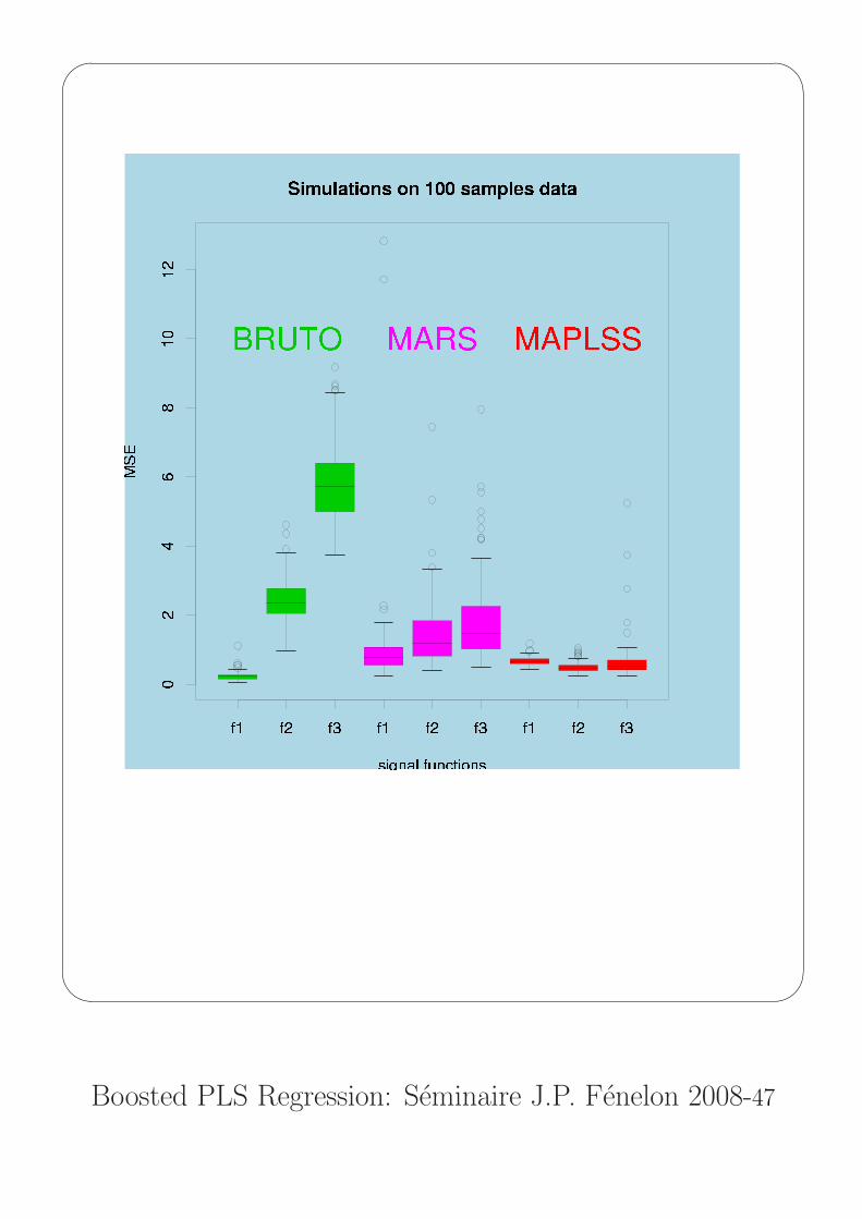
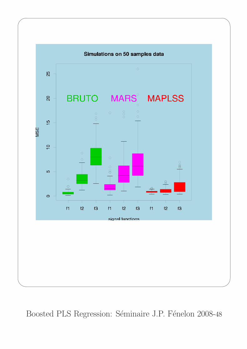
Example 3: Comparison between MAPLSS,MARS and BRUTO on simulated data
BRUTO [10, Hastie & Tibshirani]: A multi-response additive model
fitted by adaptive back-fitting using smoothing splines.
MARS[8, Friedman]: Multivariate Adaptive Regression Splines.
A two-phase process to build ANOVA style decomposition models
by fitting truncated power basis function. Variables, knots and in-
teractions are optimized simultaneously by using a GCV criterion.
Campaign of simulations:
Three signals (pure additive, one and two interactions respectively)
f1(x) = 0.1 exp(4 x1)+4
1 + exp(−20 (x2 − 0.5))+3 x3+2 x4+x5+0
10∑i=6
xi
f2(x) = 10 sin(πx1x2) + 20 (x3 − 0.5)2 + 10 x4 + 5 x5 + 0
10∑i=6
xi
f3(x) = 10 sin(πx1x2) + 20 (x3 − 0.5)2 + 20 x4x5 + 0
10∑i=6
xi
not depending on the last five variables.

'
&
$
%
Boosted PLS Regression: Seminaire J.P. Fenelon 2008-45
The model associated to the signal fj
yi = fj(xi) + εi, i = 1, . . . , n
xi ∼ U [0, 1]10 and εi ∼ N [0, 1].
100 training data sets (xi, yi)i=1,n were generated according to
n = 50, 100, 200 and j = 1, 2, 3.
For each of the 900 data sets, the goodness-of-prediction of BRUTO,
MARS and MAPLSS were measured on a new test set (ntest = n)
by computing the Mean Squared Error
MSE = n−1test
ntest∑i=1
(fj(xi)− yi)2.
These data sets were not only used to compare the domain of
efficiency of the three methods but also to calibrate the MAPLSS
tuning parameter allowing to accept or not one interaction
threshold = 20%.
'
&
$
%
Boosted PLS Regression: Seminaire J.P. Fenelon 2008-46
'
&
$
%
Boosted PLS Regression: Seminaire J.P. Fenelon 2008-47
'
&
$
%
Boosted PLS Regression: Seminaire J.P. Fenelon 2008-48
'
&
$
%
Boosted PLS Regression: Seminaire J.P. Fenelon 2008-49
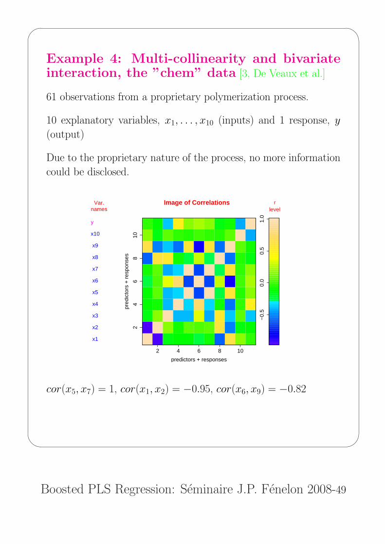
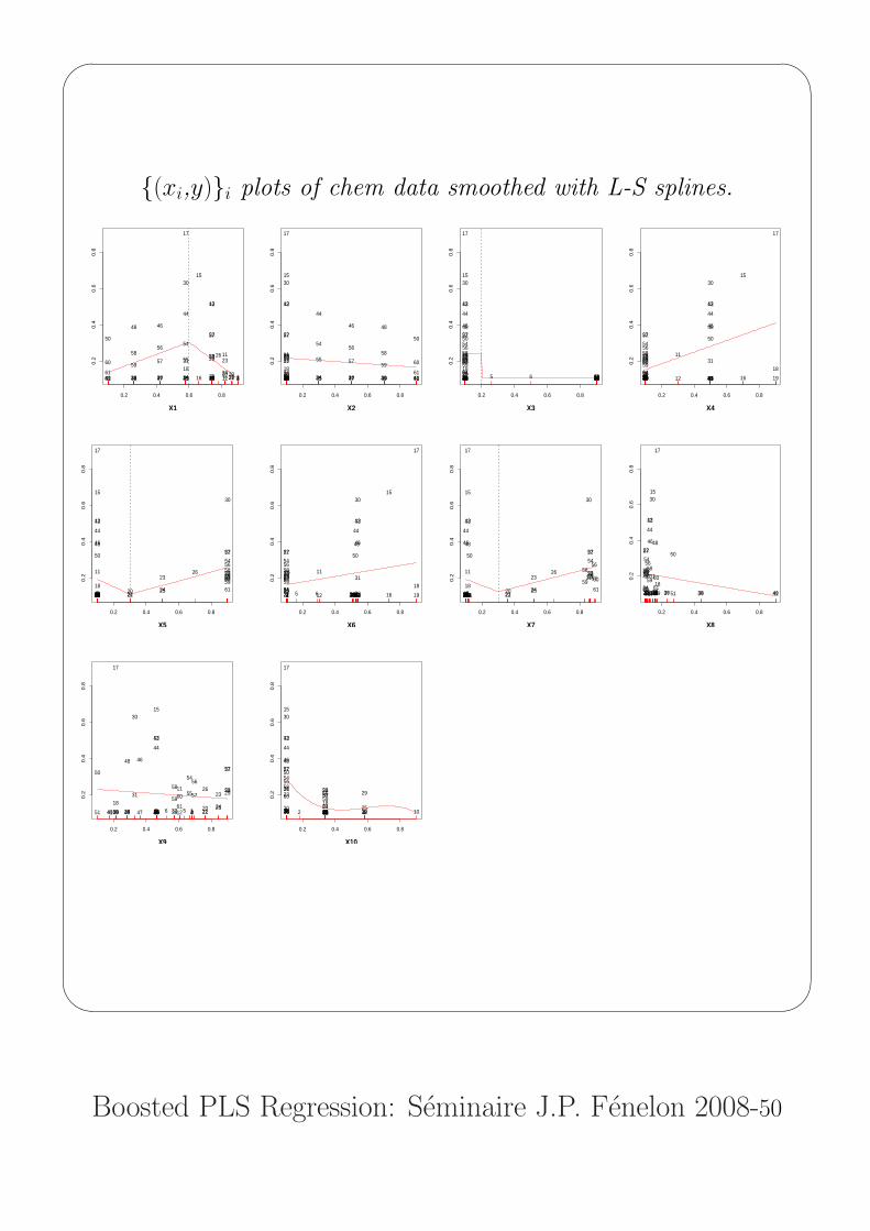
Example 4: Multi-collinearity and bivariateinteraction, the ”chem” data [3, De Veaux et al.]
61 observations from a proprietary polymerization process.
10 explanatory variables, x1, . . . , x10 (inputs) and 1 response, y
(output)
Due to the proprietary nature of the process, no more information
could be disclosed.
2 4 6 8 10
24
68
10
predictors + responses
pred
icto
rs +
res
pons
es
−0.
50.
00.
51.
0
Var.names
Image of Correlations rlevel
x1
x2
x3
x4
x5
x6
x7
x8
x9
x10
y
cor(x5, x7) = 1, cor(x1, x2) = −0.95, cor(x6, x9) = −0.82
'
&
$
%
Boosted PLS Regression: Seminaire J.P. Fenelon 2008-50
{(xi,y)}i plots of chem data smoothed with L-S splines.
0.2 0.4 0.6 0.8
0.2
0.4
0.6
0.8
X1
12345678910
11
12
13
14
15
16
17
18
19202122
23
2425
26
27
2829
30
31
32333435363738394041
42
43
44
45
46
47
48
49
50
51
52
53
54
55
56
57
58
5960
61
0.2 0.4 0.6 0.8
0.2
0.4
0.6
0.8
X2
12345678910
11
12
13
14
15
16
17
18
19202122
23
2425
26
27
2829
30
31
3233 3435 3637 3839 4041
42
43
44
45
46
47
48
49
50
51
52
53
54
55
56
57
58
59 60
61
0.2 0.4 0.6 0.8
0.2
0.4
0.6
0.8
X3
1234 5 6 78910
11
12
13
14
15
16
17
18
19202122
23
2425
26
27
2829
30
31
32333435363738394041
42
43
44
45
46
47
48
49
50
51
52
53
54
55
56
57
58
5960
61
0.2 0.4 0.6 0.8
0.2
0.4
0.6
0.8
X4
12345678910
11
12
13
14
15
16
17
18
19202122
23
2425
26
27
2829
30
31
32333435363738394041
42
43
44
45
46
47
48
49
50
51
52
53
54
55
56
57
58
5960
61
0.2 0.4 0.6 0.8
0.2
0.4
0.6
0.8
X5
12345678910
11
12
13
14
15
16
17
18
19202122
23
2425
26
27
2829
30
31
32333435363738394041
42
43
44
45
46
47
48
49
50
51
52
53
54
55
56
57
58
5960
61
0.2 0.4 0.6 0.8
0.2
0.4
0.6
0.8
X6
1234 5 6 78910
11
12
13
14
15
16
17
18
19202122
23
2425
26
27
2829
30
31
32333435363738394041
42
43
44
45
46
47
48
49
50
51
52
53
54
55
56
57
58
5960
61
0.2 0.4 0.6 0.8
0.2
0.4
0.6
0.8
X7
12345678910
11
12
13
14
15
16
17
18
19202122
23
2425
26
27
2829
30
31
32333435363738394041
42
43
44
45
46
47
48
49
50
51
52
53
54
55
56
57
58
59 60
61
0.2 0.4 0.6 0.8
0.2
0.4
0.6
0.8
X8
123456 78910
11
12
13
14
15
16
17
18
19202122
23
2425
26
27
2829
30
31
32333435 3637 3839 4041
42
43
44
45
46
47
48
49
50
51
52
53
54
55
56
57
58
59 60
61
0.2 0.4 0.6 0.8
0.2
0.4
0.6
0.8
X9
12345678910
11
12
13
14
15
16
17
18
19202122
23
2425
26
27
2829
30
31
32333435363738394041
42
43
44
45
46
47
48
49
50
51
52
53
54
55
56
57
58
5960
61
0.2 0.4 0.6 0.8
0.2
0.4
0.6
0.8
X10
1 2 3 4567 8 9 10
11
12
13
14
15
16
17
18
1920
21 22
23
24 25
26
27
28 29
30
31
32 3334 3536 3738 3940 41
42
43
44
45
46
47
48
49
50
51
52
53
54
55
56
57
58
5960
61
'
&
$
%
Boosted PLS Regression: Seminaire J.P. Fenelon 2008-51
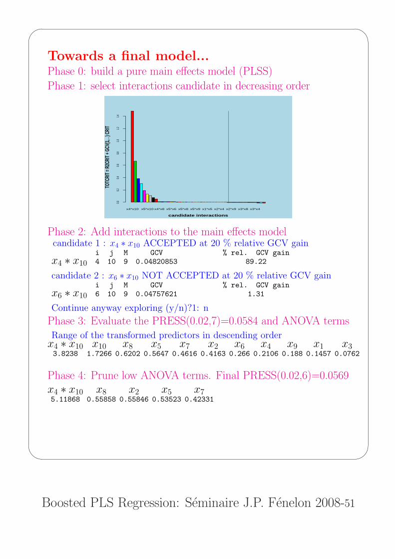
Towards a final model...Phase 0: build a pure main effects model (PLSS)
Phase 1: select interactions candidate in decreasing order
x4*x10 x5*x10 x4*x8 x5*x6 x5*x8 x5*x9 x1*x5 x2*x4 x2*x9 x3*x8 x3*x4
candidate interactions
TOTC
RIT =
R2C
RIT +
GCV
(1, . )
CRI
T
0.00.2
0.40.6
0.81.0
1.21.4
Phase 2: Add interactions to the main effects modelcandidate 1 : x4 ∗ x10 ACCEPTED at 20 % relative GCV gain
i j M GCV % rel. GCV gainx4 ∗ x10 4 10 9 0.04820853 89.22
candidate 2 : x6 ∗ x10 NOT ACCEPTED at 20 % relative GCV gaini j M GCV % rel. GCV gain
x6 ∗ x10 6 10 9 0.04757621 1.31
Continue anyway exploring (y/n)?1: n
Phase 3: Evaluate the PRESS(0.02,7)=0.0584 and ANOVA termsRange of the transformed predictors in descending order
x4 ∗ x10 x10 x8 x5 x7 x2 x6 x4 x9 x1 x33.8238 1.7266 0.6202 0.5647 0.4616 0.4163 0.266 0.2106 0.188 0.1457 0.0762
Phase 4: Prune low ANOVA terms. Final PRESS(0.02,6)=0.0569x4 ∗ x10 x8 x2 x5 x75.11868 0.55858 0.55846 0.53523 0.42331
'
&
$
%
Boosted PLS Regression: Seminaire J.P. Fenelon 2008-52
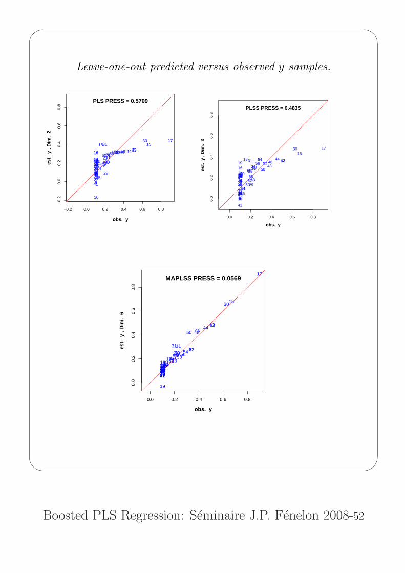
Leave-one-out predicted versus observed y samples.
−0.2 0.0 0.2 0.4 0.6 0.8
−0.
20.
00.
20.
40.
60.
8
PLS PRESS = 0.5709
obs. y
est.
y ,
Dim
. 2
12
3
4
567
8
9
10
11
12
13
14
15
16
1718
19
20
21
22
23
24
25
2627
28
29
3031
32
33
34
35
36
37
38
39
40
41
42
43
44
45
46
47
48
49
50
51
52
53
54
55
56
57
58
59
60
61
0.0 0.2 0.4 0.6 0.8
0.0
0.2
0.4
0.6
0.8
PLSS PRESS = 0.4835
obs. y
est.
y ,
Dim
. 3
1
2
34
567
8910
11
12
13
14
15
16
17
1819
20
2122
23
2425
2627
2829
30
31
32
33
34
35
36
37
38
39
40
41
42
43
44
45
46
47
48
49
50
51
52
53
54
55
56
57
58
59
60
61
0.0 0.2 0.4 0.6 0.8
0.0
0.2
0.4
0.6
0.8
MAPLSS PRESS = 0.0569
obs. y
est.
y ,
Dim
. 6
12345678910
11
12
13
14
15
16
17
18
19
202122
232425
2627
2829
30
31
3233343536373839
40
41
42
43
44
45
46
47
48
49
50
51
5253 54
55 565758
596061
'
&
$
%
Boosted PLS Regression: Seminaire J.P. Fenelon 2008-53
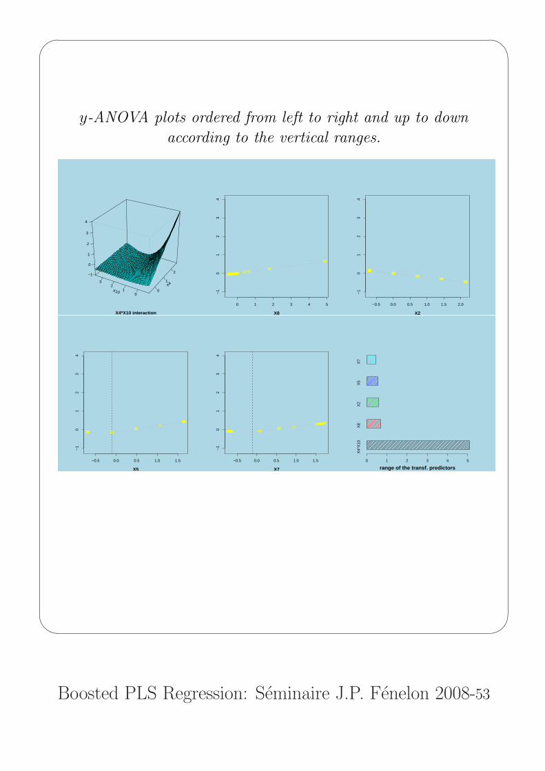
y-ANOVA plots ordered from left to right and up to down
according to the vertical ranges.
X4*X10 interaction
X4
0
1
2
X100
12
3
−1
0
1
2
3
4
0 1 2 3 4 5
−10
12
34
X8
123456 7891011121314151617181920212223242526272829 303132333435 36373839
4041
4243444546474849 50515253545556575859 6061
−0.5 0.0 0.5 1.0 1.5 2.0
−10
12
34
X2
1234567891011121314151617181920212223242526272829303132333435
36373839
4041
42434445
46474849
5051
52535455
56575859
6061
−0.5 0.0 0.5 1.0 1.5
−10
12
34
X5
12345678910111213141516171819 202122232425
262728293031
3233343536373839404142434445464748495051
52535455565758596061
−0.5 0.0 0.5 1.0 1.5
−10
12
34
X7
12345678910111213141516171819 202122232425 26
2728293031
3233343536373839404142434445464748495051
5253545556575859 6061
X4*
X10
X
8
X2
X
5
X7
range of the transf. predictors0 1 2 3 4 5
'
&
$
%
Boosted PLS Regression: Seminaire J.P. Fenelon 2008-54
References
[1] C. De Boor. A Practical Guide to Splines, Springer-Verlag, Berlin, 1978.
[2] P. Buhlmann and Bin Yu, Boosting with the L2 Loss: Regression and Classification. Journal of theAmerican Association, 98, pages 324-339, 2000.
[3] R.D. De Veaux, D.C. Psichoggios and L.H. Ungar. A comparison of two nonparametric estimationschemes: MARS and neural networks,Computers chem. Engng, Vol. 17, No. 8, pp. 819-837, 1993
[4] J.F. Durand. Local Polynomial Additive Regression through PLS and Splines: PLSS, Chemometricsand Intelligent Laboratory Systems 58, 235-246, 2001.
[5] J. F. Durand and R. Lombardo. Interactions terms in nonlinear PLS via additive spline transforma-tions. In ”Studies in Classification, Data Analysis, and Knowledge Organization”, Springer-Verlag,2003.
[6] P.H.C. Eilers and B.D. Marx Flexible smoothing with B-splines and Penalties, (with discussion).Statistical Science, 19, 89-121, 1996.
[7] J.H. Friedman. Multivariate Adaptive Regression Splines, (with discussion). The Annals of Statistics,19, 1-123, 1991.
[8] J.H. Friedman. Greedy function approximation: a gradient boosting machine. The Annals of Statis-tics, 29, 5, 1189-1232, 2001.
[9] A. Gifi. Non Linear Multivariate Analysis, J. Wiley & Sons, Chichester, 1990.
[10] T. Hastie and R. Tibshirani. Generalized additive models. Chapman and Hall, London, 1990.
[11] T. Hastie, R. Tibshirani and J.H. Friedman, The Elements of Statistical Learning, Springer, 2001.
[12] R. Lombardo, J. F. Durand and D. De Veaux. Multivariate Additive Partial Least-Squares Splines,MAPLSS. Submitted.
[13] N. Molinari, J.F. Durand and R. Sabatier. Bounded Optimal knots for Regression Splines. Compu-tational Statistics & Data Analysis, 2, 159-178, 2004.
[14] C.J. Stone. Additive regression and other nonparametric models. The Annals of Statistics, 13, 689-705, 1985.
[15] M. Sjostrom, S. Wold and B. Soderstrom, PLS discrimination plots. In E.S. Gelsema et L.N. Kanals(Eds): Pattern Recognition in Practice II. Elsevier, Amsterdam, 1986.
[16] M. Tenenhaus. La regression PLS, Theorie et Applications, Technip, Paris, 1998.
[17] J.W. Tukey, Exploratory Data Analysis. Reading Massachusetts: Addison-Wesley, 1977.
[18] H. Wold. Estimation of principal components and related models by iterative least squares. In Multi-variate Analysis, (Eds.) P.R. Krishnaiah, New York: Academic Press, 391-420, 1966.
[19] S. Wold., H. Martens and H. Wold. The mutivariate calibration problem in chemistry solved byPLS method. In: A. Ruhe, B. Kagstrom (Eds), Lecture Notes in Mathematics, Proceedings of theConference on Matrix Pencils, Springer-Verlag, Heidelberg, 286-293, 1983.