Embed Size (px)
Citation preview
Bootstrapped Meta-Learning
Sebastian FlennerhagDeepMind
Yannick SchroeckerDeepMind
Tom ZahavyDeepMind
Hado van HasseltDeepMind
David SilverDeepMind
Satinder SinghDeepMind
Abstract
Meta-learning empowers artificial intelligence to increase its efficiency by learn-ing how to learn. Unlocking this potential involves overcoming a challengingmeta-optimisation problem that often exhibits ill-conditioning, and myopic meta-objectives. We propose an algorithm that tackles these issues by letting the meta-learner teach itself. The algorithm first bootstraps a target from the meta-learner,then optimises the meta-learner by minimising the distance to that target undera chosen (pseudo-)metric. Focusing on meta-learning with gradients, we estab-lish conditions that guarantee performance improvements and show that the im-provement is related to the target distance. Thus, by controlling curvature, thedistance measure can be used to ease meta-optimization, for instance by reducingill-conditioning. Further, the bootstrapping mechanism can extend the effectivemeta-learning horizon without requiring backpropagation through all updates. Thealgorithm is versatile and easy to implement. We achieve a new state-of-the artfor model-free agents on the Atari ALE benchmark, improve upon MAML infew-shot learning, and demonstrate how our approach opens up new possibilitiesby meta-learning efficient exploration in an ε-greedy Q-learning agent.
1 Introduction
In a standard machine learning problem, a learner or agent learns a task by iteratively adjusting itsparameters under a given update rule, such as Stochastic Gradient Descent (SGD). Typically, thelearner’s update rule must be tuned manually for each task. In contrast, humans learn new tasksseamlessly by relying on previous experiences to inform their learning processes [53].
For a (machine) learner to have the same capability, it must be able to learn its update rule (or suchinductive biases). Meta-learning is one approach that learns (parts of) an update rule by applying itfor some number of steps and then evaluating the resulting performance [47, 24, 10]. For instance, awell-studied and often successful approach is to tune parameters of a gradient-based update, eitheronline during training on a single task [9, 34, 66, 68], or meta-learned over a distribution of tasks[16, 46, 18, 26, 13]. More generally, the update rule can be an arbitrary parameterised function[25, 4, 39], or the function itself can be meta-learned jointly with its parameters [2, 44].
Meta-learning is challenging because to evaluate an update rule, it must first be applied. This oftenleads to high computational costs. As a result most works optimise performance after K applicationsof the update rule and assume that this yields improved performance for the remainder of the learner’slifetime [10, 34, 35]. When this assumption fails, meta-learning suffers from a short-horizon bias[65, 35]. Similarly, optimizing the learner’s performance after K updates can fail to account for theprocess of learning, causing another form of myopia [17, 54, 12, 11]. Challenges in meta-optimisationhave been observed to cause degraded lifetime performance [32, 63], collapsed exploration [54, 12],biased learner updates [54, 69], and poor generalisation performance [65, 67, 59].
arX
iv:2
109.
0450
4v1
[cs
.LG
] 9
Sep
202
1
We argue that defining the meta-learner’s objective directly in terms of the learner’s objective—i.e. theperformance after K update steps—creates two bottlenecks in meta-optimisation. The first bottleneckis curvature: the meta-objective is constrained to the same type of geometry as the learner; the secondis myopia: the meta-objective is fundamentally limited to evaluating performance within the K-stephorizon, but ignores future learning dynamics. Our goal is to design an algorithm that removes these.
The algorithm relies on two main ideas. First, to mitigate myopia, we introduce the notion ofbootstrapping a target from the meta-learner itself or from some other update rule, what we refer toas a meta-bootstrap. This allows us to infuse information about learning dynamics into the objective.Second, to control curvature, we formulate the meta-objective in terms of minimising distance (ordivergence) to the bootstrapped target. This gives us control over the optimisation landscape. The keyinsight is that the meta-learner can learn to learn from itself by trying to match future desired updateswith fewer steps. This leads to a bootstrapping effect, where improvements beget improvements.
We present a detailed formulation in Section 3; on a high level, as in previous works, we first unrollthe meta-learned update rule for K steps to obtain the learner’s new parameters. Whereas standardmeta-objectives optimise the update rule with respect to (w.r.t.) the learner’s performance under thenew parameters, our proposed algorithm constructs the meta-objective in two steps:
1. It bootstraps a target from the learner’s new parameters. In this paper, we generate targetsby continuing to update the learner’s parameters—either under the meta-learned update ruleor another update rule—for some number of steps.
2. The learner’s new parameters—which are a function of the meta-learner’s parameters—andthe target are projected onto a matching space. A simple example is Euclidean parameterspace. To control curvature, we may choose a different (pseudo-)metric space. For instance,a common choice under probabilistic models is the Kullback-Leibler (KL) divergence.
The meta-learner is optimised by minimising distance to the bootstrapped target. We focus ongradient-based optimisation, but other optimisation routines are equally applicable. By optimisingmeta-parameters in a well-behaved space, we can drastically reduce ill-conditioning and otherphenomena that disrupt meta-optimisation. In particular, this form of Bootstrapped Meta-Gradient(BMG) enables us to infuse information about future learning dynamics without increasing thenumber of update steps to backpropagate through. In effect, the meta-learner becomes its own teacher.Because BMG optimises the meta-learner to reach a desired future target state faster, it embodiesa form of acceleration akin to Nesterov Momentum [37] and Raphson-Newton updates. We showthat BMG can guarantee performance improvements (Theorem 1) and that this guarantee can bestronger than under standard meta-gradients (Corollary 1). Empirically, we find that BMG providessubstantial performance improvements over standard meta-gradients in various settings. We obtain anew state-of-the-art result for model-free agents on Atari (Section 5.2) and improve upon MAML[16] in the few-shot setting (Section 6). Finally, we demonstrate how BMG enables new forms ofmeta-learning, exemplified by meta-learning ε-greedy exploration (Section 5.1).
2 Related Work
The idea of bootstrapping, as used here, stems from temporal difference (TD) algorithms in rein-forcement learning (RL) [55]. In these algorithms, an agent learns a value function by using its ownfuture predictions as targets. Bootstrapping has recently been introduced in the self-supervised setting[21, 20]. In this paper, we introduce the idea of bootstrapping in the context of meta-learning, wherea meta-learner learns about an update rule by generating future targets from it.
Our approach to target matching is related to methods in multi-task meta-learning [17, 38] thatmeta-learn an initialisation for SGD by minimising the Euclidean distance to task-optimal parameters.BMG generalise this concept by allowing for arbitrary meta-parameters, matching functions, andtarget bootstraps. It is further related the more general concept of self-referential meta-learning[47, 48], where the meta-learned update rule is used to optimise its own meta-objective.
Target matching under KL divergences results in a form of distillation [23], where an online network(student) is encouraged to match a target network (teacher). In a typical setup, the target is either afixed (set of) expert(s) [23, 45] or a moving aggregation of current experts [57, 20], whereas BMGbootstraps a target by following an update rule. Finally, BMG is loosely inspired by trust-regionmethods that introduce a distance function to regularize gradient updates [41, 51, 58, 22].
2
3 Bootstrapped Meta-Gradients
x
x(K)
w
w
x
πx(K)
πx
(x, f(x))
(s, πx(s))
∇wµ(x,x(K)(w)) π
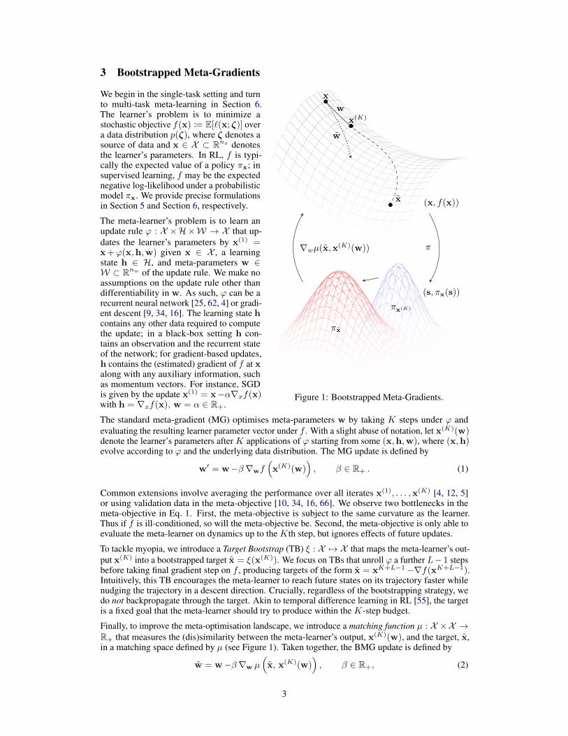
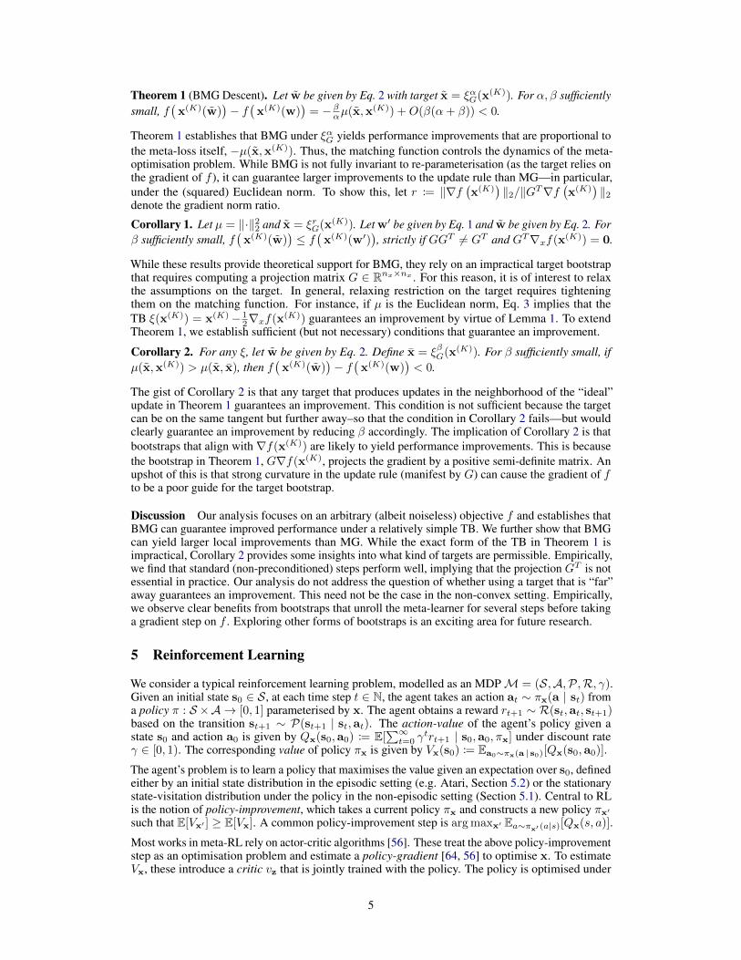
Figure 1: Bootstrapped Meta-Gradients.
We begin in the single-task setting and turnto multi-task meta-learning in Section 6.The learner’s problem is to minimize astochastic objective f(x) := E[`(x; ζ)] overa data distribution p(ζ), where ζ denotes asource of data and x ∈ X ⊂ Rnx denotesthe learner’s parameters. In RL, f is typi-cally the expected value of a policy πx; insupervised learning, f may be the expectednegative log-likelihood under a probabilisticmodel πx. We provide precise formulationsin Section 5 and Section 6, respectively.
The meta-learner’s problem is to learn anupdate rule ϕ : X ×H×W → X that up-dates the learner’s parameters by x(1) =x+ϕ(x,h,w) given x ∈ X , a learningstate h ∈ H, and meta-parameters w ∈W ⊂ Rnw of the update rule. We make noassumptions on the update rule other thandifferentiability in w. As such, ϕ can be arecurrent neural network [25, 62, 4] or gradi-ent descent [9, 34, 16]. The learning state hcontains any other data required to computethe update; in a black-box setting h con-tains an observation and the recurrent stateof the network; for gradient-based updates,h contains the (estimated) gradient of f at xalong with any auxiliary information, suchas momentum vectors. For instance, SGDis given by the update x(1) = x−α∇xf(x)with h = ∇xf(x), w = α ∈ R+.
The standard meta-gradient (MG) optimises meta-parameters w by taking K steps under ϕ andevaluating the resulting learner parameter vector under f . With a slight abuse of notation, let x(K)(w)denote the learner’s parameters after K applications of ϕ starting from some (x,h,w), where (x,h)evolve according to ϕ and the underlying data distribution. The MG update is defined by
w′ = w−β∇wf(x(K)(w)
), β ∈ R+ . (1)
Common extensions involve averaging the performance over all iterates x(1), . . . ,x(K) [4, 12, 5]or using validation data in the meta-objective [10, 34, 16, 66]. We observe two bottlenecks in themeta-objective in Eq. 1. First, the meta-objective is subject to the same curvature as the learner.Thus if f is ill-conditioned, so will the meta-objective be. Second, the meta-objective is only able toevaluate the meta-learner on dynamics up to the Kth step, but ignores effects of future updates.
To tackle myopia, we introduce a Target Bootstrap (TB) ξ : X 7→ X that maps the meta-learner’s out-put x(K) into a bootstrapped target x = ξ(x(K)). We focus on TBs that unroll ϕ a further L− 1 stepsbefore taking final gradient step on f , producing targets of the form x = xK+L−1−∇f(xK+L−1).Intuitively, this TB encourages the meta-learner to reach future states on its trajectory faster whilenudging the trajectory in a descent direction. Crucially, regardless of the bootstrapping strategy, wedo not backpropagate through the target. Akin to temporal difference learning in RL [55], the targetis a fixed goal that the meta-learner should try to produce within the K-step budget.
Finally, to improve the meta-optimisation landscape, we introduce a matching function µ : X ×X →R+ that measures the (dis)similarity between the meta-learner’s output, x(K)(w), and the target, x,in a matching space defined by µ (see Figure 1). Taken together, the BMG update is defined by
w = w−β∇w µ(x, x(K)(w)
), β ∈ R+, (2)
3
where the gradient is with respect to the second argument of µ. Thus, BMG describes a family ofalgorithms based on the choice of matching function µ and TB ξ. In particular, MG is a special case ofBMG under matching function µ(x,x(K)) = ‖x−x(K) ‖22 and TB ξ(x(K)) = x(K)− 1
2∇xf(x(K)),since the bootstrapped meta-gradient reduces to the standard meta-gradient:
∇w∥∥∥x− x(K)(w)
∥∥∥2
2= −2D
(x− x(K)
)= D∇xf
(x(K)
)= ∇wf
(x(K)(w)
), (3)
where D denotes the (transposed) Jacobian of x(K)(w). For other matching functions and targetstrategies, BMG produces different meta-updates compared to MG. We discuss these choices below.
Matching Function Of primary concern to us are deep neural networks that output a probabilisticdistribution, πx. A common pseudo-metric over a space of probability distributions is the Kullback-Leibler (KL) divergence. For instance, Natural Gradients [3] point in the direction of steepest descentunder the KL-divergence. In neural networks, this is often approximated through a KL-regularizationterm [41], which is an instance of Mirror Descent [7]. KL-divergences also arise naturally in RLalgorithms [28], often in the form of trust-region methods [51, 52, 1]. Hence, a natural starting pointis to consider KL-divergences between the target and the iterate, e.g. µ(x,x(K)) = KL (πx ‖ πx(K)).In actor-critic algorithms [56], the policy defines only part of the agent—the value function definesthe other. Thus, we also consider a composite matching function over both policy and value function.
Target Bootstrap We analyze conditions under which BMG guarantees performance improvementsin Section 4 and find that the target should co-align with the gradient direction. Thus, in this paper wefocus on gradient-based TBs and find that they perform well empirically. As with matching functions,this is a small subset of all possible choices; we leave the exploration of other choices for future work.
4 Performance Guarantees
In this analysis, we restrict attention to the noise-less setting (true expectations) and consider 1-steptarget updates. In this setting, we ask three questions: (1) what local performance guarantees areprovided by MG? (2) What performance guarantees can BMG provide? (3) How do these guaranteesrelate to each other? To answer these questions, we analyse how the performance around f(x(K)(w))changes by updating w either under standard meta-gradients (Eq. 1) or bootstrapped meta-gradients(Eq. 2). Throughout, we assume that f and x(K) are Lipschitz.
First, consider improvements under the MG update. In online optimisation, the MG update can achievestrong convergence guarantees if the problem is well-behaved [60], with similar guarantees in themulti-task setting [6, 30, 13]. A central component of these results is that the MG update guaranteesa local improvement in the objective. Lemma 1 below presents this result in our setting, with thefollowing notation: let ‖u ‖A :=
√〈u, Au〉 for any square real matrix A. Let GT = DTD ∈
Rnx×nx , with D :=[∂∂w x(K)(w)
]T ∈ Rnw×nx . Note that∇wf(x(K)(w)) = D∇xf(x(K)).
Lemma 1 (MG Descent). Let w′ be given by Eq. 1. For β sufficiently small, f(x(K)(w′)
)−
f(x(K)(w)
)= −β‖∇xf(x(K))‖2GT +O(β2) < 0.
We defer all proofs to Appendix A. Lemma 1 relates the gains obtained under standard meta-gradientsto the local gradient norm of the objective. A key property of the meta-gradient is that, because themeta-objective is given by f , it is not scale-free [c.f. 50], nor invariant to re-parameterisation. Thus, iff is a highly non-linear function, the meta-gradient can vary widely, preventing efficient performanceimprovement. Next, we turn to BMG. To facilitate the analysis we assume µ differentiable, Lipschitzcontinuous and convex in its second argument, with 0 being its minimum:
µ(x, z) = 0 ⇐⇒ x = z, µ(x, z) ≥ 0 ∀x, z ∈ X . (4)
To obtain performance improvement guarantees, we must place some structure on the TB. This isbecause if x points away from the solution space, updating the meta-learner in this direction will notimprove the update rule. For instance, this can happen if ϕ is a black-box meta-learner and the targetis generated by unrolling ϕ. To establish a descent guarantee, we first analyse a gradient-based TB ofthe form ξαG(x(K)) := x(K)−αGT∇xf(x(K)), α ∈ R+, which provides an intuitive guarantee.
4
Theorem 1 (BMG Descent). Let w be given by Eq. 2 with target x = ξαG(x(K)). For α, β sufficientlysmall, f
(x(K)(w)
)− f
(x(K)(w)
)= −β
αµ(x,x(K)) +O(β(α+ β)) < 0.
Theorem 1 establishes that BMG under ξαG yields performance improvements that are proportional tothe meta-loss itself, −µ(x,x(K)). Thus, the matching function controls the dynamics of the meta-optimisation problem. While BMG is not fully invariant to re-parameterisation (as the target relies onthe gradient of f ), it can guarantee larger improvements to the update rule than MG—in particular,under the (squared) Euclidean norm. To show this, let r := ‖∇f
(x(K)
)‖2/‖GT∇f
(x(K)
)‖2
denote the gradient norm ratio.
Corollary 1. Let µ = ‖·‖22 and x = ξrG(x(K)). Let w′ be given by Eq. 1 and w be given by Eq. 2. Forβ sufficiently small, f
(x(K)(w)
)≤ f
(x(K)(w′)
), strictly if GGT 6= GT and GT∇xf(x(K)) = 0.
While these results provide theoretical support for BMG, they rely on an impractical target bootstrapthat requires computing a projection matrix G ∈ Rnx×nx . For this reason, it is of interest to relaxthe assumptions on the target. In general, relaxing restriction on the target requires tighteningthem on the matching function. For instance, if µ is the Euclidean norm, Eq. 3 implies that theTB ξ(x(K)) = x(K)− 1
2∇xf(x(K)) guarantees an improvement by virtue of Lemma 1. To extendTheorem 1, we establish sufficient (but not necessary) conditions that guarantee an improvement.
Corollary 2. For any ξ, let w be given by Eq. 2. Define x = ξβG(x(K)). For β sufficiently small, ifµ(x,x(K)) > µ(x, x), then f
(x(K)(w)
)− f
(x(K)(w)
)< 0.
The gist of Corollary 2 is that any target that produces updates in the neighborhood of the “ideal”update in Theorem 1 guarantees an improvement. This condition is not sufficient because the targetcan be on the same tangent but further away–so that the condition in Corollary 2 fails—but wouldclearly guarantee an improvement by reducing β accordingly. The implication of Corollary 2 is thatbootstraps that align with ∇f(x(K)) are likely to yield performance improvements. This is becausethe bootstrap in Theorem 1, G∇f(x(K), projects the gradient by a positive semi-definite matrix. Anupshot of this is that strong curvature in the update rule (manifest by G) can cause the gradient of fto be a poor guide for the target bootstrap.
Discussion Our analysis focuses on an arbitrary (albeit noiseless) objective f and establishes thatBMG can guarantee improved performance under a relatively simple TB. We further show that BMGcan yield larger local improvements than MG. While the exact form of the TB in Theorem 1 isimpractical, Corollary 2 provides some insights into what kind of targets are permissible. Empirically,we find that standard (non-preconditioned) steps perform well, implying that the projection GT is notessential in practice. Our analysis do not address the question of whether using a target that is “far”away guarantees an improvement. This need not be the case in the non-convex setting. Empirically,we observe clear benefits from bootstraps that unroll the meta-learner for several steps before takinga gradient step on f . Exploring other forms of bootstraps is an exciting area for future research.
5 Reinforcement Learning
We consider a typical reinforcement learning problem, modelled as an MDPM = (S,A,P,R, γ).Given an initial state s0 ∈ S , at each time step t ∈ N, the agent takes an action at ∼ πx(a | st) froma policy π : S ×A → [0, 1] parameterised by x. The agent obtains a reward rt+1 ∼ R(st,at, st+1)based on the transition st+1 ∼ P(st+1 | st,at). The action-value of the agent’s policy given astate s0 and action a0 is given by Qx(s0,a0) := E[
∑∞t=0 γ
trt+1 | s0,a0, πx] under discount rateγ ∈ [0, 1). The corresponding value of policy πx is given by Vx(s0) := Ea0∼πx(a | s0)[Qx(s0,a0)].
The agent’s problem is to learn a policy that maximises the value given an expectation over s0, definedeither by an initial state distribution in the episodic setting (e.g. Atari, Section 5.2) or the stationarystate-visitation distribution under the policy in the non-episodic setting (Section 5.1). Central to RLis the notion of policy-improvement, which takes a current policy πx and constructs a new policy πx′
such that E[Vx′ ] ≥ E[Vx]. A common policy-improvement step is arg maxx′ Ea∼πx′ (a|s)[Qx(s, a)].
Most works in meta-RL rely on actor-critic algorithms [56]. These treat the above policy-improvementstep as an optimisation problem and estimate a policy-gradient [64, 56] to optimise x. To estimateVx, these introduce a critic vz that is jointly trained with the policy. The policy is optimised under
5
2 4 8 16 32 64 outer = 0 outer = 0.1K+L
1 1 1 3 1 3 7 1 3 7 15 1 3 7 15 31 1 3 7 15 31 1 3 7 15 31K
0.0
0.5
1.0
1.5
Ret
urn
afte
r 10
M s
teps
(Mill
ions
) Bootstrapped Meta-gradients Meta-gradients No MG
0.05
0.15
0.25
Rew
./Ste
p
0 100000 200000 300000Env Steps into Cycle
0.0
0.2
0.4
0.6
Ent
ropy
Rat
e
No MG BMG MG
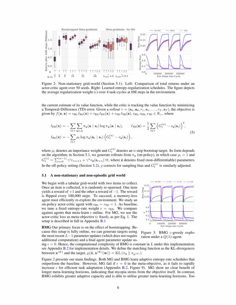
Figure 2: Non-stationary grid-world (Section 5.1). Left: Comparison of total returns under anactor-critic agent over 50 seeds. Right: Learned entropy-regularization schedules. The figure depictsthe average regularization weight (ε) over 4 task-cycles at 6M steps in the environment.
the current estimate of its value function, while the critic is tracking the value function by minimizinga Temporal-Difference (TD) error. Given a rollout τ = (s0,a0, r1, s1, . . . , rT , sT ), the objective isgiven by f(x, z) = εPG `PG(x) + εEN `EN(x) + εTD `TD(z), εPG, εEN, εTD ∈ R+, where
`EN(x) = −∑t∈τ
∑a∈A
πx(a | st) log πx(a | st), `TD(z) =1
2
∑t∈τ
(G
(n)t − vz(st)
)2
,
`PG(x) = −∑t∈τ
ρt log πx(at | st)(G
(n)t − vz(st)
),
(5)
where ρt denotes an importance weight and G(n)t denotes an n-step bootstrap target. Its form depends
on the algorithm; in Section 5.1, we generate rollouts from πx (on-policy), in which case ρt = 1 andG
(n)t =
∑(n−1)i=0 γirt+i+1 + γnvz(st+n)∀t, where z denotes fixed (non-differentiable) parameters.
In the off-policy setting (Section 5.2), ρ corrects for sampling bias and G(n)t is similarly adjusted.
5.1 A non-stationary and non-episodic grid world
0.05
0.15
0.25
Rew
./Ste
p
0 100000 200000 300000Env Steps into Cycle
0.1
0.2
0.3
0.4
No MG L=16 L=32 L=128
Figure 3: BMG ε-greedy explo-ration under a Q(λ)-agent.
We begin with a tabular grid-world with two items to collect.Once an item is collected, it is randomly re-spawned. One itemyields a reward of +1 and the other a reward of−1. The rewardis flipped every 100,000 steps. To succeed, a memory-lessagent must efficiently re-explore the environment. We study anon-policy actor-critic agent with εPG = εTD = 1. As baseline,we tune a fixed entropy-rate weight ε = εEN. We compareagainst agents that meta-learn ε online. For MG, we use theactor-critic loss as meta-objective (ε fixed), as per Eq. 1. Thesetup is described in full in Appendix B.1
BMG Our primary focus is on the effect of bootstrapping. Be-cause this setup is fully online, we can generate targets usingthe most recentL−1 parameter updates (which does not requireadditional computation) and a final agent parameter update us-ing ε = 0. Hence, the computational complexity of BMG is constant in L under this implementation;see Appendix B.2 for implementation details. We define the matching function as the KL-divergencesbetween x(K) and the target, µ(x,x(K)(w)) = KL (πx ‖ πx(K)).
Figure 2 presents our main findings. Both MG and BMG learn adaptive entropy-rate schedules thatoutperform the baseline. However, MG fail if ε = 0 in the meta-objective, as it fails to rapidlyincrease ε for efficient task adaptation (Appendix B.2, Figure 9). MG show no clear benefit oflonger meta-learning horizons, indicating that myopia stems from the objective itself. In contrast,BMG exhibits greater adaptive capacity and is able to utilise greater meta-learning horizons. Too
6
Games with absolute difference > 0.5
0
10
20
30
40
Rel
ativ
e pe
rfor
man
ce
0 50M 100M 150M 200MLearning frames
0
1
2
3
4
5
6
Med
ian
hum
an n
orm
aliz
ed s
core
IMPALA192%, [8]
Metagradient287%, [44]
STACX364%, [45]
LASER431%, [32]
BMG611% (ours)BMG w. KL & V, L=4
BMG w. KL & VBMG w. KLSTACX*
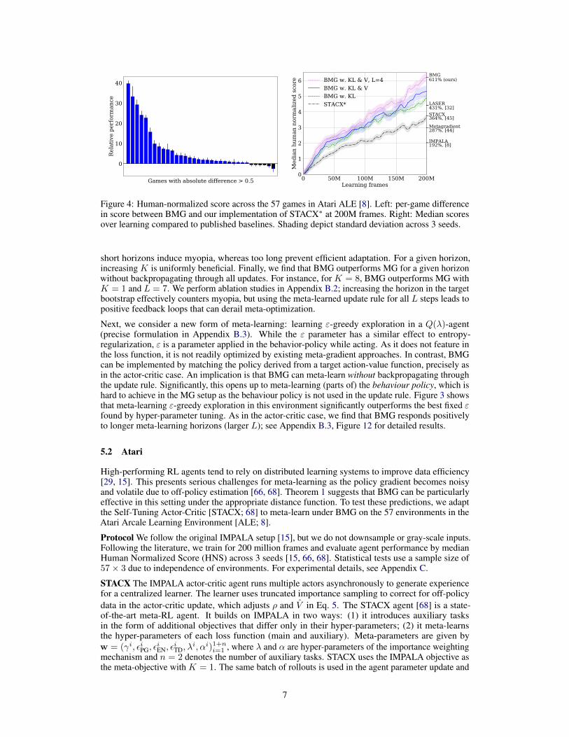
Figure 4: Human-normalized score across the 57 games in Atari ALE [8]. Left: per-game differencein score between BMG and our implementation of STACX∗ at 200M frames. Right: Median scoresover learning compared to published baselines. Shading depict standard deviation across 3 seeds.
short horizons induce myopia, whereas too long prevent efficient adaptation. For a given horizon,increasing K is uniformly beneficial. Finally, we find that BMG outperforms MG for a given horizonwithout backpropagating through all updates. For instance, for K = 8, BMG outperforms MG withK = 1 and L = 7. We perform ablation studies in Appendix B.2; increasing the horizon in the targetbootstrap effectively counters myopia, but using the meta-learned update rule for all L steps leads topositive feedback loops that can derail meta-optimization.
Next, we consider a new form of meta-learning: learning ε-greedy exploration in a Q(λ)-agent(precise formulation in Appendix B.3). While the ε parameter has a similar effect to entropy-regularization, ε is a parameter applied in the behavior-policy while acting. As it does not feature inthe loss function, it is not readily optimized by existing meta-gradient approaches. In contrast, BMGcan be implemented by matching the policy derived from a target action-value function, precisely asin the actor-critic case. An implication is that BMG can meta-learn without backpropagating throughthe update rule. Significantly, this opens up to meta-learning (parts of) the behaviour policy, which ishard to achieve in the MG setup as the behaviour policy is not used in the update rule. Figure 3 showsthat meta-learning ε-greedy exploration in this environment significantly outperforms the best fixed εfound by hyper-parameter tuning. As in the actor-critic case, we find that BMG responds positivelyto longer meta-learning horizons (larger L); see Appendix B.3, Figure 12 for detailed results.
5.2 Atari
High-performing RL agents tend to rely on distributed learning systems to improve data efficiency[29, 15]. This presents serious challenges for meta-learning as the policy gradient becomes noisyand volatile due to off-policy estimation [66, 68]. Theorem 1 suggests that BMG can be particularlyeffective in this setting under the appropriate distance function. To test these predictions, we adaptthe Self-Tuning Actor-Critic [STACX; 68] to meta-learn under BMG on the 57 environments in theAtari Arcale Learning Environment [ALE; 8].
Protocol We follow the original IMPALA setup [15], but we do not downsample or gray-scale inputs.Following the literature, we train for 200 million frames and evaluate agent performance by medianHuman Normalized Score (HNS) across 3 seeds [15, 66, 68]. Statistical tests use a sample size of57× 3 due to independence of environments. For experimental details, see Appendix C.
STACX The IMPALA actor-critic agent runs multiple actors asynchronously to generate experiencefor a centralized learner. The learner uses truncated importance sampling to correct for off-policydata in the actor-critic update, which adjusts ρ and V in Eq. 5. The STACX agent [68] is a state-of-the-art meta-RL agent. It builds on IMPALA in two ways: (1) it introduces auxiliary tasksin the form of additional objectives that differ only in their hyper-parameters; (2) it meta-learnsthe hyper-parameters of each loss function (main and auxiliary). Meta-parameters are given byw = (γi, εiPG, ε
iEN, ε
iTD, λ
i, αi)1+ni=1 , where λ and α are hyper-parameters of the importance weighting
mechanism and n = 2 denotes the number of auxiliary tasks. STACX uses the IMPALA objective asthe meta-objective with K = 1. The same batch of rollouts is used in the agent parameter update and
7
SGDL2
L=1
RMSL2
L=1
RMSKL
L=1
RMSKL & V
L=1
RMSKL & V
L=4
3.5
4.0
4.5
5.0
5.5
6.0
Hum
an n
orm
aliz
ed s
core
KL KL & V
20
25
30
35
40
Epi
sode
Ret
urn
(100
0x)
L1248
2 0 2 4Normalized mean episode return
0.00
0.05
0.10
0.15
0.20
0.25
0.30
0.35
0.40
Den
sity
KL & VKL-SKLV
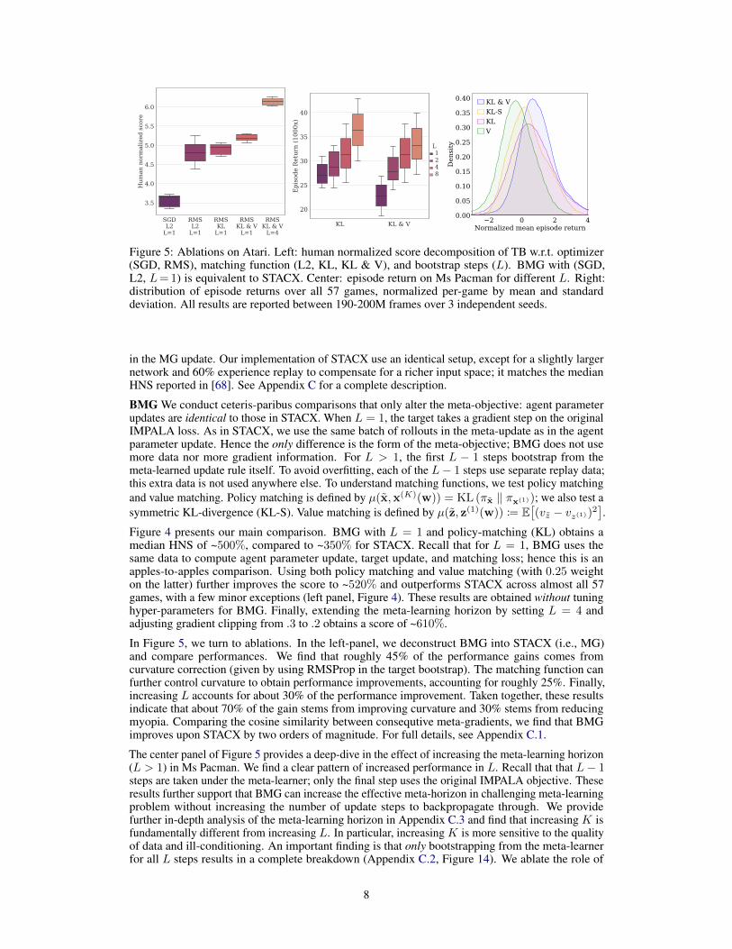
Figure 5: Ablations on Atari. Left: human normalized score decomposition of TB w.r.t. optimizer(SGD, RMS), matching function (L2, KL, KL & V), and bootstrap steps (L). BMG with (SGD,L2, L= 1) is equivalent to STACX. Center: episode return on Ms Pacman for different L. Right:distribution of episode returns over all 57 games, normalized per-game by mean and standarddeviation. All results are reported between 190-200M frames over 3 independent seeds.
in the MG update. Our implementation of STACX use an identical setup, except for a slightly largernetwork and 60% experience replay to compensate for a richer input space; it matches the medianHNS reported in [68]. See Appendix C for a complete description.
BMG We conduct ceteris-paribus comparisons that only alter the meta-objective: agent parameterupdates are identical to those in STACX. When L = 1, the target takes a gradient step on the originalIMPALA loss. As in STACX, we use the same batch of rollouts in the meta-update as in the agentparameter update. Hence the only difference is the form of the meta-objective; BMG does not usemore data nor more gradient information. For L > 1, the first L − 1 steps bootstrap from themeta-learned update rule itself. To avoid overfitting, each of the L− 1 steps use separate replay data;this extra data is not used anywhere else. To understand matching functions, we test policy matchingand value matching. Policy matching is defined by µ(x,x(K)(w)) = KL (πx ‖ πx(1)); we also test asymmetric KL-divergence (KL-S). Value matching is defined by µ(z, z(1)(w)) := E
[(vz − vz(1))2
].
Figure 4 presents our main comparison. BMG with L = 1 and policy-matching (KL) obtains amedian HNS of ~500%, compared to ~350% for STACX. Recall that for L = 1, BMG uses thesame data to compute agent parameter update, target update, and matching loss; hence this is anapples-to-apples comparison. Using both policy matching and value matching (with 0.25 weighton the latter) further improves the score to ~520% and outperforms STACX across almost all 57games, with a few minor exceptions (left panel, Figure 4). These results are obtained without tuninghyper-parameters for BMG. Finally, extending the meta-learning horizon by setting L = 4 andadjusting gradient clipping from .3 to .2 obtains a score of ~610%.
In Figure 5, we turn to ablations. In the left-panel, we deconstruct BMG into STACX (i.e., MG)and compare performances. We find that roughly 45% of the performance gains comes fromcurvature correction (given by using RMSProp in the target bootstrap). The matching function canfurther control curvature to obtain performance improvements, accounting for roughly 25%. Finally,increasing L accounts for about 30% of the performance improvement. Taken together, these resultsindicate that about 70% of the gain stems from improving curvature and 30% stems from reducingmyopia. Comparing the cosine similarity between consequtive meta-gradients, we find that BMGimproves upon STACX by two orders of magnitude. For full details, see Appendix C.1.
The center panel of Figure 5 provides a deep-dive in the effect of increasing the meta-learning horizon(L > 1) in Ms Pacman. We find a clear pattern of increased performance in L. Recall that that L− 1steps are taken under the meta-learner; only the final step uses the original IMPALA objective. Theseresults further support that BMG can increase the effective meta-horizon in challenging meta-learningproblem without increasing the number of update steps to backpropagate through. We providefurther in-depth analysis of the meta-learning horizon in Appendix C.3 and find that increasing K isfundamentally different from increasing L. In particular, increasing K is more sensitive to the qualityof data and ill-conditioning. An important finding is that only bootstrapping from the meta-learnerfor all L steps results in a complete breakdown (Appendix C.2, Figure 14). We ablate the role of
8
replay in meta-updates Appendix C.2. We find that standard MG generally degrades as we increasethe amount of replay, but that BMG can successfully leverage replay in the target bootstrap.
The right panel of Figure 5 studies the effect of the matching function. Overall, we find that jointpolicy and value matching exhibits superior performance. Interestingly, while recent work [58, 22]suggest that reversing or using a symmetric KL-objective can yield improvements, we do not findthis to be the case here. Using only value-matching results in worse performance, as it only optimisesfor efficient policy evaluation but lacks an explicit signal for optimising the policy improvementoperator. Finally, we conduct detailed analysis of scalability. We find that while BMG is 20% slowerfor K = 1, L = 1 due to the target bootstrap, it is 200% faster when MG uses K = 4 and BMG usesK = 1, L = 3. For more detailed results, including effect of network size, see Appendix C.4.
6 Multi-Task Few-Shot Learning
100 200 300 400 500 600Steps (1000x)
50
55
60
65
70
75
80
Valid
atio
n ac
cura
cy (%
)BMG, KL-1BMG, KL-2BMG, KL-SMAML
KL-1 KL-2 KL-S58
60
62
64
66
68
Accu
racy
(%)
L1510
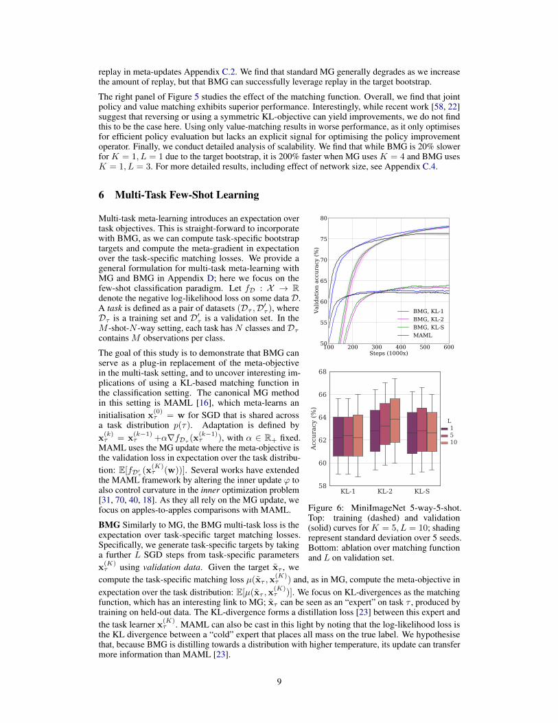
Figure 6: MiniImageNet 5-way-5-shot.Top: training (dashed) and validation(solid) curves for K = 5, L = 10; shadingrepresent standard deviation over 5 seeds.Bottom: ablation over matching functionand L on validation set.
Multi-task meta-learning introduces an expectation overtask objectives. This is straight-forward to incorporatewith BMG, as we can compute task-specific bootstraptargets and compute the meta-gradient in expectationover the task-specific matching losses. We provide ageneral formulation for multi-task meta-learning withMG and BMG in Appendix D; here we focus on thefew-shot classification paradigm. Let fD : X → Rdenote the negative log-likelihood loss on some data D.A task is defined as a pair of datasets (Dτ ,D′τ ), whereDτ is a training set and D′τ is a validation set. In theM -shot-N -way setting, each task has N classes and Dτcontains M observations per class.
The goal of this study is to demonstrate that BMG canserve as a plug-in replacement of the meta-objectivein the multi-task setting, and to uncover interesting im-plications of using a KL-based matching function inthe classification setting. The canonical MG methodin this setting is MAML [16], which meta-learns aninitialisation x
(0)τ = w for SGD that is shared across
a task distribution p(τ). Adaptation is defined byx
(k)τ = x
(k−1)τ +α∇fDτ (x
(k−1)τ ), with α ∈ R+ fixed.
MAML uses the MG update where the meta-objective isthe validation loss in expectation over the task distribu-tion: E[fD′
τ(x
(K)τ (w))]. Several works have extended
the MAML framework by altering the inner update ϕ toalso control curvature in the inner optimization problem[31, 70, 40, 18]. As they all rely on the MG update, wefocus on apples-to-apples comparisons with MAML.
BMG Similarly to MG, the BMG multi-task loss is theexpectation over task-specific target matching losses.Specifically, we generate task-specific targets by takinga further L SGD steps from task-specific parametersx
(K)τ using validation data. Given the target xτ , we
compute the task-specific matching loss µ(xτ ,x(K)τ ) and, as in MG, compute the meta-objective in
expectation over the task distribution: E[µ(xτ ,x(K)τ )]. We focus on KL-divergences as the matching
function, which has an interesting link to MG; xτ can be seen as an “expert” on task τ , produced bytraining on held-out data. The KL-divergence forms a distillation loss [23] between this expert andthe task learner x(K)
τ . MAML can also be cast in this light by noting that the log-likelihood loss isthe KL divergence between a “cold” expert that places all mass on the true label. We hypothesisethat, because BMG is distilling towards a distribution with higher temperature, its update can transfermore information than MAML [23].
9
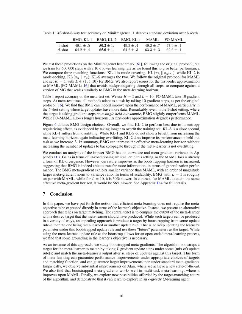
Table 1: M -shot-5-way test accuracy on MiniImagenet. ± denotes standard deviation over 5 seeds.
BMG, KL-1 BMG, KL-2 BMG, KL-s MAML FO-MAML1-shot 49.1± .5 50.2± 1. 49.3± .4 49.2± .7 47.9± .15-shot 64.2± .4 65.0± 1. 64.2± .3 63.3± .3 62.6± .1
We test these predictions on the MiniImagenet benchmark [61], following the original protocol, butwe train for 600 000 steps with a 10× lower learning rate as we found this to give better performance.We compare three matching functions: KL-1 is mode-covering, KL (πx ‖ πx(K)), while KL-2 ismode-seeking, KL (πx ‖ πx); KL-S averages the two. We follow the original protocol for MAMLand set K = 5, with L ∈ {1, 5, 10} for BMG. We also report scores for the first-order approximationto MAML [FO-MAML; 16] that avoids backpropagating through all steps, to compare against aversion of MG that scales similarly to BMG in the meta-learning horizon.
Table 1 report accuracy on the meta-test set. We use K = 5 and L = 10. FO-MAML take 10 gradientsteps. At meta-test time, all methods adapt to a task by taking 10 gradient steps, as per the originalprotocol [16]. We find that BMG can indeed improve upon the performance of MAML, particularly inthe 5-shot setting where target updates have more data. Remarkably, even in the 1-shot setting, wherethe target is taking gradient steps on a single held-out sample, BMG slightly outperforms MAML.While FO-MAML allows longer horizons, its first-order approximation degrades performance.
Figure 6 ablates BMG design choices. Overall, we find KL-2 to perform best due to its entropyregularizing effect, as evidenced by taking longer to overfit the training set. KL-S is a close second,while KL-1 suffers from overfitting. While KL-1 and KL-S do not show a benefit from increasing themeta-learning horizon, again indicating overfitting, KL-2 does improve its performance on held-outtask as we increase L. In summary, BMG can increase the effective meta-learning horizon withoutincreasing the number of updates to backpropagate through if the meta-learner is not overfitting.
We conduct an analysis of the impact BMG has on curvature and meta-gradient variance in Ap-pendix D.3. Gains in terms of ill-conditioning are smaller in this setting, as the MAML loss is alreadya form of KL-divergence. However, curvature improves as the bootstrapping horizon is increased,suggesting that BMG is indeed able to transfer more information, in terms of generalization perfor-mance. The BMG meta-gradient exhibits smaller variance than MAML, with an order of magnitudelarger meta-gradient norm to variance ratio. In terms of scalability, BMG with L = 1 is roughlyon par with MAML, while for L = 10, it is 50% slower. In contrast, for MAML to attain the sameeffective meta-gradient horizon, it would be 56% slower. See Appendix D.4 for full details.
7 Conclusion
In this paper, we have put forth the notion that efficient meta-learning does not require the meta-objective to be expressed directly in terms of the learner’s objective. Instead, we present an alternativeapproach that relies on target matching. The central tenet is to compare the output of the meta-learnerwith a desired target that the meta-learner should have produced. While such targets can be producedin a variety of ways, an appealing approach is produce a target by bootstrapping from some updaterule–either the one being meta-learned or another update rule. That is, to keep updating the learner’sparameter under this bootstrapped update rule and use these “future” parameters as the target. Whileusing the meta-learned update rule as the bootstrap allows for an open-ended meta-learning process,we find that some grounding in the learner’s objective is necessary.
As an instance of this approach, we study bootstrapped meta-gradients. The algorithm bootstraps atarget for the meta-learner to match by taking L gradient update steps under some (mix of) updaterule(s) and match the meta-learner’s output after K steps of updates against this target. This formof meta-learning can guarantee performance improvements under appropriate choices of targetsand matching function, and can guarantee larger improvements than under standard meta-gradients.Empirically, we observe substantial improvements on Atari, where we achieve a new state-of-the-art.We also find that bootstrapped meta-gradients works well in multi-task meta-learning, where itimproves upon MAML. Finally, we explore new possibilities afforded by the target-matching natureof the algorithm, and demonstrate that it can learn to explore in an ε-greedy Q-learning agent.
10
Acknowledgments and Disclosure of Funding
The authors would like to thank Guillaume Desjardins, Junhyuk Oh, Luisa Zintgraf, Razvan Pascanu,and Nando de Freitas for insightful feedback on earlier versions of this paper. This work was fundedby DeepMind.
References[1] A. Abdolmaleki, J. T. Springenberg, Y. Tassa, R. Munos, N. Heess, and M. Riedmiller. Maxi-
mum a Posteriori Policy Optimisation. In International Conference on Learning Representations,2018.
[2] F. Alet, M. F. Schneider, T. Lozano-Perez, and L. P. Kaelbling. Meta-Learning CuriosityAlgorithms. In International Conference on Learning Representations, 2020.
[3] S.-I. Amari. Natural Gradient Works Efficiently in Learning. Neural computation, 10(2):251–276, 1998.
[4] M. Andrychowicz, M. Denil, S. Gómez, M. W. Hoffman, D. Pfau, T. Schaul, and N. de Freitas.Learning to Learn by Gradient Descent by Gradient Descent. In Advances in Neural InformationProcessing Systems, 2016.
[5] A. Antoniou, H. Edwards, and A. J. Storkey. How to Train Your MAML. In InternationalConference on Learning Representations, 2019.
[6] M.-F. Balcan, M. Khodak, and A. Talwalkar. Provable Guarantees for Gradient-Based Meta-Learning. In International Conference on Machine Learning, 2019.
[7] A. Beck and M. Teboulle. Mirror Descent and Nonlinear Projected Subgradient Methods forConvex Optimization. Operations Research Letters, 31:167–175, 2003.
[8] M. G. Bellemare, Y. Naddaf, J. Veness, and M. Bowling. The Arcade Learning Environment: AnEvaluation Platform for General Agents. Journal of Artificial Intelligence Research, 47:253–279,2013.
[9] Y. Bengio. Gradient-Based Optimization of Hyperparameters. Neural computation, 12(8):1889–1900, 2000.
[10] Y. Bengio, S. Bengio, and J. Cloutier. Learning a Synaptic Learning Rule. Université deMontréal, Département d’informatique et de recherche opérationnelle, 1991.
[11] Y. Cao, T. Chen, Z. Wang, and Y. Shen. Learning to Optimize in Swarms. Advances in NeuralInformation Processing Systems, 2019.
[12] Y. Chen, M. W. Hoffman, S. G. Colmenarejo, M. Denil, T. P. Lillicrap, and N. de Freitas.Learning to learn for Global Optimization of Black Box Functions. In Advances in NeuralInformation Processing Systems, 2016.
[13] G. Denevi, D. Stamos, C. Ciliberto, and M. Pontil. Online-Within-Online Meta-Learning. InAdvances in Neural Information Processing Systems, 2019.
[14] J. Deng, W. Dong, R. Socher, L.-J. Li, K. Li, and L. Fei-Fei. Imagenet: A Large-ScaleHierarchical Image Database. In Computer Vision and Pattern Recognition, 2009.
[15] L. Espeholt, H. Soyer, R. Munos, K. Simonyan, V. Mnih, T. Ward, Y. Doron, V. Firoiu, T. Harley,I. Dunning, et al. Impala: Scalable Distributed Deep-RL with Importance Weighted Actor-Learner Architectures. In International Conference on Machine Learning, 2018.
[16] C. Finn, P. Abbeel, and S. Levine. Model-Agnostic Meta-Learning for Fast Adaptation of DeepNetworks. In International Conference on Machine Learning, 2017.
[17] S. Flennerhag, P. G. Moreno, N. D. Lawrence, and A. Damianou. Transferring Knowledgeacross Learning Processes. In International Conference on Learning Representations, 2019.
11
[18] S. Flennerhag, A. A. Rusu, R. Pascanu, F. Visin, H. Yin, and R. Hadsell. Meta-Learning withWarped Gradient Descent. In International Conference on Learning Representations, 2020.
[19] E. Grant, C. Finn, S. Levine, T. Darrell, and T. L. Griffiths. Recasting Gradient-Based Meta-Learning as Hierarchical Bayes. In International Conference on Learning Representations,2018.
[20] J.-B. Grill, F. Strub, F. Altché, C. Tallec, P. Richemond, E. Buchatskaya, C. Doersch,B. Avila Pires, Z. Guo, M. Gheshlaghi Azar, B. Piot, k. kavukcuoglu, R. Munos, and M. Valko.Bootstrap Your Own Latent: A New Approach to Self-Supervised Learning. In Advances inNeural Information Processing Systems, 2020.
[21] Z. D. Guo, B. A. Pires, B. Piot, J.-B. Grill, F. Altché, R. Munos, and M. G. Azar. BootstrapLatent-Predictive Representations for Multitask Reinforcement Learning. In InternationalConference on Machine Learning, 2020.
[22] M. Hessel, I. Danihelka, F. Viola, A. Guez, S. Schmitt, L. Sifre, T. Weber, D. Silver, andH. van Hasselt. Muesli: Combining Improvements in Policy Optimization. arXiv preprintarXiv:2104.06159, 2021.
[23] G. Hinton, O. Vinyals, and J. Dean. Distilling the Knowledge in a Neural Network. arXivpreprint arXiv:1503.02531, 2015.
[24] G. E. Hinton and D. C. Plaut. Using Fast Weights to Deblur Old Memories. In CognitiveScience Society, 1987.
[25] S. Hochreiter, A. S. Younger, and P. R. Conwell. Learning To Learn Using Gradient Descent.In International Conference on Artificial Neural Networks, 2001.
[26] G. Jerfel, E. Grant, T. Griffiths, and K. A. Heller. Reconciling Meta-Learning and ContinualLearning with Online Mixtures of Tasks. In Advances in Neural Information Processing Systems,2019.
[27] N. P. Jouppi, C. Young, N. Patil, D. Patterson, G. Agrawal, R. Bajwa, S. Bates, S. Bhatia,N. Boden, and A. Borchers. In-Datacenter Performance Analysis of a Tensor Processing Unit.In International Symposium on Computer Architecture, 2017.
[28] S. M. Kakade. A Natural Policy Gradient. In Advances in Neural Information ProcessingSystems, 2001.
[29] S. Kapturowski, G. Ostrovski, J. Quan, R. Munos, and W. Dabney. Recurrent ExperienceReplay in Distributed Reinforcement Learning. In International Conference on LearningRepresentations, 2018.
[30] M. Khodak, M.-F. F. Balcan, and A. S. Talwalkar. Adaptive Gradient-Based Meta-LearningMethods. Advances in Neural Information Processing Systems, 2019.
[31] Y. Lee and S. Choi. Gradient-Based Meta-Learning with Learned Layerwise Metric andSubspace. In International Conference on Machine Learning, 2018.
[32] K. Lv, S. Jiang, and J. Li. Learning Gradient Descent: Better Generalization and LongerHorizons. In International Conference on Machine Learning, 2017.
[33] M. C. Machado, M. G. Bellemare, E. Talvitie, J. Veness, M. Hausknecht, and M. Bowling.Revisiting the Arcade Learning Environment: Evaluation Protocols and Open Problems forGeneral Agents. Journal of Artificial Intelligence Research, 61:523–562, 2018.
[34] D. Maclaurin, D. Duvenaud, and R. Adams. Gradient-Based Hyperparameter OptimizationThrough Reversible Learning. In International conference on machine learning, pages 2113–2122. PMLR, 2015.
[35] L. Metz, N. Maheswaranathan, J. Nixon, D. Freeman, and J. Sohl-Dickstein. Understandingand Correcting Pathologies in the Training of Learned Optimizers. In International Conferenceon Machine Learning, 2019.
12
[36] V. Mnih, K. Kavukcuoglu, D. Silver, A. Graves, I. Antonoglou, D. Wierstra, and M. Riedmiller.Playing Atari with Deep Reinforcement Learning. arXiv preprint arXiv:1312.5602, 2013.
[37] Y. Nesterov. A Method for Solving the Convex Programming Problem with Convergence RateO(1/k2). Proceedings of the USSR Academy of Sciences, 269:543–547, 1983.
[38] A. Nichol, J. Achiam, and J. Schulman. On First-Order Meta-Learning Algorithms. arXivpreprint ArXiv:1803.02999, 2018.
[39] J. Oh, M. Hessel, W. M. Czarnecki, Z. Xu, H. P. van Hasselt, S. Singh, and D. Silver. DiscoveringReinforcement Learning Algorithms. In Advances in Neural Information Processing Systems,volume 33, 2020.
[40] E. Park and J. B. Oliva. Meta-Curvature. In Advances in Neural Information Processing Systems,2019.
[41] R. Pascanu and Y. Bengio. Revisiting Natural Gradient for Deep Networks. In InternationalConference on Learning Representations, 2014.
[42] J. Peng and R. J. Williams. Incremental Multi-Step Q-Learning. In International Conferenceon Machine Learning, 1994.
[43] S. Ravi and H. Larochelle. Optimization as a Model for Few-Shot Learning. In InternationalConference on Learning Representations, 2017.
[44] E. Real, C. Liang, D. R. So, and Q. V. Le. AutoML-Zero: Evolving Machine LearningAlgorithms From Scratch. In International Conference on Machine Learning, 2020.
[45] A. A. Rusu, S. G. Colmenarejo, C. Gulcehre, G. Desjardins, J. Kirkpatrick, R. Pascanu, V. Mnih,K. Kavukcuoglu, and R. Hadsell. Policy Distillation. arXiv preprint arXiv:1511.06295, 2015.
[46] A. A. Rusu, D. Rao, J. Sygnowski, O. Vinyals, R. Pascanu, S. Osindero, and R. Hadsell.Meta-Learning with Latent Embedding Optimization. In International Conference on LearningRepresentations, 2019.
[47] J. Schmidhuber. Evolutionary Principles in Self-Referential Learning. PhD thesis, TechnischeUniversität München, 1987.
[48] J. Schmidhuber. A ’self-referential’ weight matrix. In International Conference on ArtificialNeural Networks, pages 446–450. Springer, 1993.
[49] S. Schmitt, M. Hessel, and K. Simonyan. Off-Policy Actor-Critic with Shared ExperienceReplay. In International Conference on Machine Learning, 2020.
[50] N. N. Schraudolph. Local Gain Adaptation in Stochastic Gradient Descent. In InternationalConference on Artificial Neural Networks, 1999.
[51] J. Schulman, S. Levine, P. Abbeel, M. Jordan, and P. Moritz. Trust Region Policy Optimization.In International Conference on Machine Learning, 2015.
[52] J. Schulman, F. Wolski, P. Dhariwal, A. Radford, and O. Klimov. Proximal Policy OptimizationAlgorithms. arXiv preprint arXiv:1707.06347, 2017.
[53] E. S. Spelke and K. D. Kinzler. Core Knowledge. Developmental science, 10(1):89–96, 2007.
[54] B. C. Stadie, G. Yang, R. Houthooft, X. Chen, Y. Duan, Y. Wu, P. Abbeel, and I. Sutskever.Some Considerations on Learning to Explore via Meta-Reinforcement Learning. In Advancesin Neural Information Processing Systems, 2018.
[55] R. S. Sutton. Learning to Predict by the Methods of Temporal Differences. Machine learning,3(1):9–44, 1988.
[56] R. S. Sutton, D. A. McAllester, S. P. Singh, and Y. Mansour. Policy Gradient Methods forReinforcement Learning with Function Approximation. In Advances in Neural InformationProcessing Systems, volume 99, 1999.
13
[57] Y. W. Teh, V. Bapst, W. M. Czarnecki, J. Quan, J. Kirkpatrick, R. Hadsell, N. Heess, andR. Pascanu. Distral: Robust Multitask Reinforcement Learning. In Advances in NeuralInformation Processing Systems, 2017.
[58] M. Tomar, L. Shani, Y. Efroni, and M. Ghavamzadeh. Mirror Descent Policy Optimization.arXiv preprint arXiv:2005.09814, 2020.
[59] E. Triantafillou, T. Zhu, V. Dumoulin, P. Lamblin, U. Evci, K. Xu, R. Goroshin, C. Gelada,K. Swersky, and P.-A. Manzagol. Meta-Dataset: A Dataset of Datasets for Learning to Learnfrom Few Examples. International Conference on Learning Representations, 2020.
[60] T. van Erven and W. M. Koolen. MetaGrad: Multiple Learning Rates in Online Learning. InAdvances in Neural Information Processing Systems, 2016.
[61] O. Vinyals, C. Blundell, T. Lillicrap, K. Kavukcuoglu, and D. Wierstra. Matching Networks forOne Shot Learning. In Advances in Neural Information Processing Systems, 2016.
[62] J. X. Wang, Z. Kurth-Nelson, D. Tirumala, H. Soyer, J. Z. Leibo, R. Munos, C. Blundell,D. Kumaran, and M. Botvinick. Learning to Reinforcement Learn. In Annual Meeting of theCognitive Science Society, 2016.
[63] O. Wichrowska, N. Maheswaranathan, M. W. Hoffman, S. G. Colmenarejo, M. Denil, N. de Fre-itas, and J. Sohl-Dickstein. Learned Optimizers that Scale and Generalize. In InternationalConference on Machine Learning, 2017.
[64] R. J. Williams and J. Peng. Function Optimization using Connectionist Reinforcement LearningAlgorithms. Connection Science, 3(3):241–268, 1991.
[65] Y. Wu, M. Ren, R. Liao, and R. B. Grosse. Understanding Short-Horizon Bias in StochasticMeta-Optimization. In International Conference on Learning Representations, 2018.
[66] Z. Xu, H. P. van Hasselt, and D. Silver. Meta-Gradient Reinforcement Learning. In Advancesin Neural Information Processing Systems, 2018.
[67] M. Yin, G. Tucker, M. Zhou, S. Levine, and C. Finn. Meta-Learning without Memorization. InInternational Conference on Learning Representations, 2020.
[68] T. Zahavy, Z. Xu, V. Veeriah, M. Hessel, J. Oh, H. P. van Hasselt, D. Silver, and S. Singh. ASelf-Tuning Actor-Critic Algorithm. Advances in Neural Information Processing Systems, 33,2020.
[69] Z. Zheng, J. Oh, and S. Singh. On Learning Intrinsic Rewards for Policy Gradient Methods.Advances in Neural Information Processing Systems, 2018.
[70] L. Zintgraf, K. Shiarli, V. Kurin, K. Hofmann, and S. Whiteson. Fast Context Adaptation viaMeta-Learning. In International Conference on Machine Learning, 2019.
14
Bootstrapped Meta-Learning: Appendix
Contents
Appendix A: proofs accompanying Section 4.Appendix B: non-stationary Grid-World (Section 5.1).Appendix C: ALE Atari (Section 5.2).Appendix D: Multi-task meta-learning, Few-Shot Learning on MiniImagenet (Section 6).
A Proofs
This section provides complete proofs for the results in Section 4. Throughout, we assume that(x(0),h(0),w) is given and write x := x(0), h := h(0). We assume that h evolves according to someprocess that maps a history H(k) := (x(0),h(0), . . . ,x(k−1),h(k−1),x(k)) into a new learner stateh(k), including any sampling of data (c.f. Section 3). Recall that we restrict attention to the noiselesssetting, and hence updates are considered in expectation. We define the map x(K)(w) by
x(1) = x(0) +ϕ(x(0),h(0),w
)x(2) = x(1) +ϕ
(x(1),h(1),w
)...
x(K) = x(K−1) +ϕ(x(K−1),h(K−1),w
).
The derivative ∂∂w x(K)(w) differentiates through each step of this process [25]. As previously
stated, we assume f is Lipschitz and that x(K) is Lipschitz w.r.t. w; we assume that µ satisfies Eq. 4.We are now in a position to prove results from the main text. We re-state them for convenience.
Lemma 1 (MG Descent). Let w′ be given by Eq. 1. For β sufficiently small, f(x(K)(w′)
)−
f(x(K)(w)
)= −β‖∇xf(x(K))‖2GT +O(β2) < 0.
Proof. Define g := ∇xf(x(K)(w)). The meta-gradient at (x,h,w) is given by ∇wf(x(K)(w)) =D g. Under Eq. 1, we find w′ = w−βD g. By first-order Taylor Series Expansion of f around(x,h,w′) with respect to w:
f(x(K)(w′)
)= f
(x(K)(w)
)+ 〈D g,w′−w〉+O(‖w′−w ‖22)
= f(x(K)(w)
)− β〈D g, D g〉+O(β2)
= f(x(K)(w)
)− β‖g ‖2GT +O(β2).
Noting that ‖g ‖2GT ≥ 0 by virtue of positive semi-definiteness of G completes the proof. �
Theorem 1 (BMG Descent). Let w be given by Eq. 2 with target x = ξαG(x(K)). For β sufficientlysmall, f
(x(K)(w)
)− f
(x(K)(w)
)< 0. Further, for α, β sufficiently small, f
(x(K)(w)
)−
f(x(K)(w)
)= −β
αµ(x,x(K)) +O(β(α+ β)) < 0.
Proof. The bootstrapped meta-gradient at (x,h,w) is given by
∇wµ(x, x(K)(w)
)= D u, where u := ∇zµ
(x, z
)∣∣∣z=x(K)
.
Under Eq. 2, we find w = w−βD u. Define g := ∇xf(x(K)). By first-order Taylor SeriesExpansion of f around (x,h, w) with respect to w:
15
f(x(K)(w)
)= f
(x(K)(w)
)+ 〈D g, w −w〉+O(‖w −w ‖22)
= f(x(K)(w)
)− β〈D g, D u〉+O(β2)
= f(x(K)(w)
)− β〈u, GT g〉+O(β2). (6)
To bound the inner product, by convexity in µ(x, ·):
µ(x, x) ≥ µ(x,x(K)) +⟨u, x− x(K)
⟩≥ µ(x,x(K)) +
⟨u, x(K)−αGT g−x(K)
⟩≥ µ(x,x(K))− α
⟨u, GT g
⟩.
Using that µ(x, x) = 0 by virtue Eq. 4, we find −µ(x,x(K)) ≥ −α〈g, GT u〉. Further, fromEq. 4, we have that µ(x,x(K)) > 0. Therefore, −〈g, GT u〉 < 0. Thus, for β sufficiently smallthe residual vanishes and f
(x(K)(w)
)− f
(x(K)(w)
)< 0, as was to be proved. For the final
part of the proof, from a first-order Taylor series expansion of µ(x, ·), we have −βαµ(x,x(K)) =
−β〈u, GT g〉+O(αβ). Then, in Eq. 6, substitute −β⟨u, GT g
⟩for −β
αµ(x,x(K)) +O(αβ). �
We now prove that, controlling for scale, BMG can yield larger performance gains than MG. Recallthat ξαG(x(K)) = x(K)−αGT∇f x(K). Consider ξrG, with r := ‖∇f(x(K))‖2/‖GT∇f(x(K))‖2.
Corollary 1. Let µ = ‖ · ‖22 and x = ξrG(x(K)). Let w′ be given by Eq. 1 and w be given by Eq. 2.For β sufficiently small, f
(x(K)(w)
)≤ f
(x(K)(w′)
), with strict inequality if GGT 6= GT .
Proof. Let g := ∇xf(x(K)
). By Lemma 1, f
(x(K)(w′)
)−f(x(K)(w)
)= −β〈GT g,g〉+O(β2).
From Theorem 1, with µ = ‖ · ‖22, f(x(K)(w)
)−f(x(K)(w)
)= −r〈GT g, GT g〉+O(β(α+β)).
For β sufficiently small, the inner products dominate and we have
f(x(K)(w)
)− f
(x(K)(w′)
)≈ −β
(r〈GT g, GT g〉 − 〈GT g,g〉
).
To determine the sign of the expression in parenthesis, consider the problem
maxv∈Rnx
〈GT g,v〉 s.t. ‖v ‖2 ≤ 1.
Form the Lagrangian L(v, λ) := 〈GT g,v〉 − λ(‖v ‖2 − 1). Solve for first-order conditions:
GT g−λ v∗
‖v∗ ‖2= 0 =⇒ v∗ =
‖v∗ ‖2λ
GT g .
If λ = 0, then we must have ‖v∗ ‖20, which clearly is not an optimal solution. Complementary slack-ness then implies ‖v∗ ‖2 = 1, which gives λ = ‖v∗ ‖2‖GT g ‖2 and hence v∗ = GT g /‖GT g ‖2.By virtue of being the maximiser, v∗ attains a higher function value than any other v with ‖v ‖2 ≤ 1,in particular v = g /‖g ‖2. Evaluating the objective at these two points gives
〈GT g, GT g〉‖GT g ‖2
≥ 〈GT g,g〉‖g ‖2
=⇒ r〈GT g, GT g〉 ≥ 〈GT g,g〉,
where we use that r = ‖g ‖2/‖GT g ‖2 by definition. Thus f(x(K)(w)
)≤ f
(x(K)(w′)
), with
strict inequality if GGT 6= GT and GT g 6= 0. �
Corollary 2. For any ξ, let w be given by Eq. 2. Define x = ξβG(x(K)). Let µ be convex in its secondargument. For β sufficiently small, if µ(x,x(K)) > µ(x, x), then f
(x(K)(w)
)− f
(x(K)(w)
)< 0.
16
Proof. Define u := ∇zµ(x, z)∣∣z=x(K) . From the proof of Theorem 1, we have that for α = β,
f(x(K)(w)
)− f
(x(K)(w)
)= −β〈u, GT g〉+O(β2) = 〈u, x− x(K)〉+O(β2).
Since u is the gradient of the BMG objective under x, it does not immediately follow that this guar-antees an improvement. From convexity of µ, we have that µ(x, x) ≥ µ(x,x(K)) +
⟨u, x− x(K)
⟩.
Thus, if µ(x,x(K)) > µ(x, x), it follows that⟨u, x− x(K)
⟩≤ 0. �
B Non-Stationary non-episodic reinforcement learning
B.1 Setup
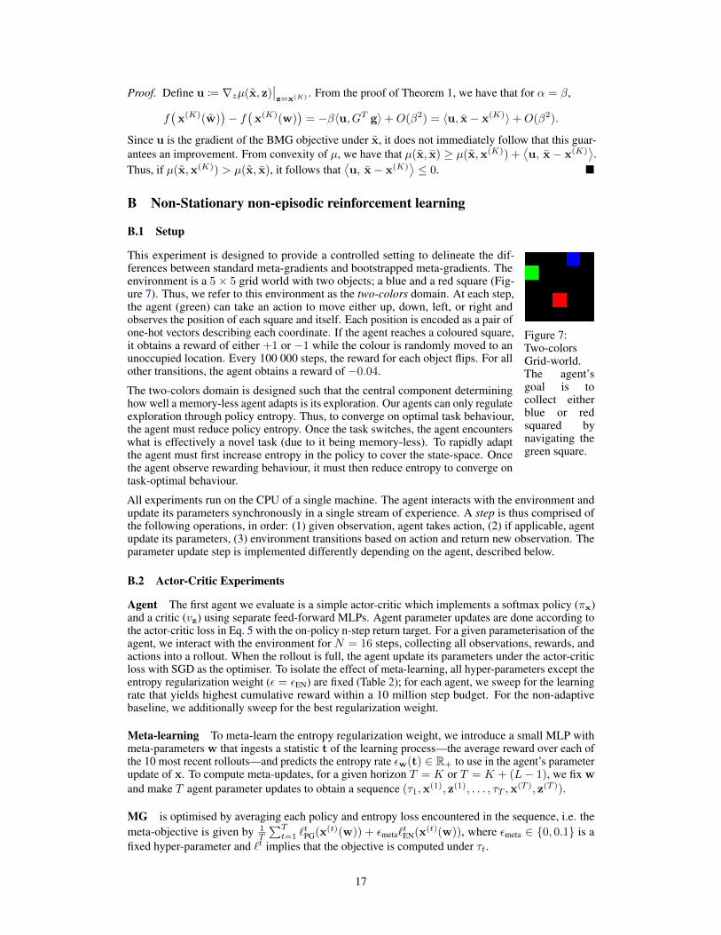
Figure 7:Two-colorsGrid-world.The agent’sgoal is tocollect eitherblue or redsquared bynavigating thegreen square.
This experiment is designed to provide a controlled setting to delineate the dif-ferences between standard meta-gradients and bootstrapped meta-gradients. Theenvironment is a 5× 5 grid world with two objects; a blue and a red square (Fig-ure 7). Thus, we refer to this environment as the two-colors domain. At each step,the agent (green) can take an action to move either up, down, left, or right andobserves the position of each square and itself. Each position is encoded as a pair ofone-hot vectors describing each coordinate. If the agent reaches a coloured square,it obtains a reward of either +1 or −1 while the colour is randomly moved to anunoccupied location. Every 100 000 steps, the reward for each object flips. For allother transitions, the agent obtains a reward of −0.04.
The two-colors domain is designed such that the central component determininghow well a memory-less agent adapts is its exploration. Our agents can only regulateexploration through policy entropy. Thus, to converge on optimal task behaviour,the agent must reduce policy entropy. Once the task switches, the agent encounterswhat is effectively a novel task (due to it being memory-less). To rapidly adaptthe agent must first increase entropy in the policy to cover the state-space. Oncethe agent observe rewarding behaviour, it must then reduce entropy to converge ontask-optimal behaviour.
All experiments run on the CPU of a single machine. The agent interacts with the environment andupdate its parameters synchronously in a single stream of experience. A step is thus comprised ofthe following operations, in order: (1) given observation, agent takes action, (2) if applicable, agentupdate its parameters, (3) environment transitions based on action and return new observation. Theparameter update step is implemented differently depending on the agent, described below.
B.2 Actor-Critic Experiments
Agent The first agent we evaluate is a simple actor-critic which implements a softmax policy (πx)and a critic (vz) using separate feed-forward MLPs. Agent parameter updates are done according tothe actor-critic loss in Eq. 5 with the on-policy n-step return target. For a given parameterisation of theagent, we interact with the environment for N = 16 steps, collecting all observations, rewards, andactions into a rollout. When the rollout is full, the agent update its parameters under the actor-criticloss with SGD as the optimiser. To isolate the effect of meta-learning, all hyper-parameters except theentropy regularization weight (ε = εEN) are fixed (Table 2); for each agent, we sweep for the learningrate that yields highest cumulative reward within a 10 million step budget. For the non-adaptivebaseline, we additionally sweep for the best regularization weight.
Meta-learning To meta-learn the entropy regularization weight, we introduce a small MLP withmeta-parameters w that ingests a statistic t of the learning process—the average reward over each ofthe 10 most recent rollouts—and predicts the entropy rate εw(t) ∈ R+ to use in the agent’s parameterupdate of x. To compute meta-updates, for a given horizon T = K or T = K + (L− 1), we fix wand make T agent parameter updates to obtain a sequence (τ1,x
(1), z(1), . . . , τT ,x(T ), z(T )).
MG is optimised by averaging each policy and entropy loss encountered in the sequence, i.e. themeta-objective is given by 1
T
∑Tt=1 `
tPG(x(t)(w)) + εmeta`
tEN(x(t)(w)), where εmeta ∈ {0, 0.1} is a
fixed hyper-parameter and `t implies that the objective is computed under τt.
17
0.0 0.2 0.4 0.6 0.8 1.0Steps 1e7
0.0
0.5
1.0
1.5
Cum
ulat
ive
Rew
ard
(Mill
ions
)
(a) Fixed entropy-regularization
0.0 0.2 0.4 0.6 0.8 1.0Steps 1e7
0.0
0.5
1.0
1.5
Cum
ulat
ive
Rew
ard
(Mill
ions
)
K=1K=3K=7K=15K=31
(b) Meta-gradients
0.0 0.2 0.4 0.6 0.8 1.0Steps 1e7
0.0
0.5
1.0
1.5
Cum
ulat
ive
Rew
ard
(Mill
ions
)
K=1K=3K=7K=15K=31
(c) Meta-gradients + regularization
0.0 0.2 0.4 0.6 0.8 1.0Steps 1e7
0.0
0.5
1.0
1.5
Cum
ulat
ive
Rew
ard 1e6 K+L=2
0.0 0.2 0.4 0.6 0.8 1.0Steps 1e7
K+L=4
0.0 0.2 0.4 0.6 0.8 1.0Steps 1e7
K+L=8
0.0 0.2 0.4 0.6 0.8 1.0Steps 1e7
K+L=16
0.0 0.2 0.4 0.6 0.8 1.0Steps 1e7
K+L=32K=1K=3K=7K=15K=31
(d) Bootstrapped meta-gradients
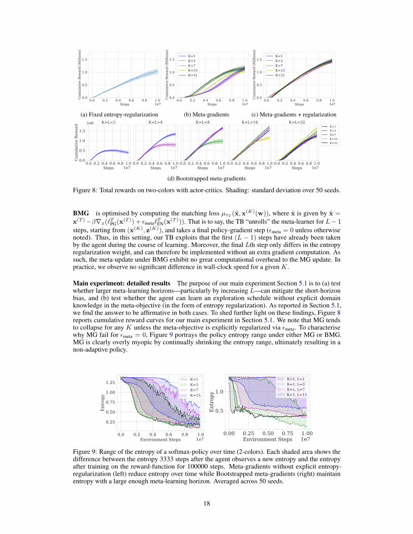
Figure 8: Total rewards on two-colors with actor-critics. Shading: standard deviation over 50 seeds.
BMG is optimised by computing the matching loss µτT (x,x(K)(w)), where x is given by x =x(T )−β∇x(`TPG(x(T )) + εmeta`
TEN(x(T ))). That is to say, the TB “unrolls” the meta-learner for L− 1
steps, starting from (x(K), z(K)), and takes a final policy-gradient step (εmeta = 0 unless otherwisenoted). Thus, in this setting, our TB exploits that the first (L − 1) steps have already been takenby the agent during the course of learning. Moreover, the final Lth step only differs in the entropyregularization weight, and can therefore be implemented without an extra gradient computation. Assuch, the meta-update under BMG exhibit no great computational overhead to the MG update. Inpractice, we observe no significant difference in wall-clock speed for a given K.
Main experiment: detailed results The purpose of our main experiment Section 5.1 is to (a) testwhether larger meta-learning horizons—particularly by increasing L—can mitigate the short-horizonbias, and (b) test whether the agent can learn an exploration schedule without explicit domainknowledge in the meta-objective (in the form of entropy regularization). As reported in Section 5.1,we find the answer to be affirmative in both cases. To shed further light on these findings, Figure 8reports cumulative reward curves for our main experiment in Section 5.1. We note that MG tendsto collapse for any K unless the meta-objective is explicitly regularized via εmeta. To characterisewhy MG fail for εmeta = 0, Figure 9 portrays the policy entropy range under either MG or BMG.MG is clearly overly myopic by continually shrinking the entropy range, ultimately resulting in anon-adaptive policy.
0.0 0.2 0.4 0.6 0.8 1.0Environment Steps 1e7
0.25
0.50
0.75
1.00
1.25
Ent
ropy
K=1K=3K=7K=15
0.00 0.25 0.50 0.75 1.00Environment Steps 1e7
0.5
1.0
Ent
ropy
K=1, L=1K=1, L=3K=1, L=7K=1, L=15
Figure 9: Range of the entropy of a softmax-policy over time (2-colors). Each shaded area shows thedifference between the entropy 3333 steps after the agent observes a new entropy and the entropyafter training on the reward-function for 100000 steps. Meta-gradients without explicit entropy-regularization (left) reduce entropy over time while Bootstrapped meta-gradients (right) maintainentropy with a large enough meta-learning horizon. Averaged across 50 seeds.
18
0.0 0.2 0.4 0.6 0.8 1.0Environment Steps 1e7
0.2
0.4
0.6
0.8
1.0
Ent
ropy
-loss
wei
ght
meta =meta = 0meta = 0.1
0.0 0.2 0.4 0.6 0.8 1.0Environment Steps 1e7
0.0
0.2
0.4
0.6
0.8
1.0
Ent
ropy
-loss
wei
ght
meta =meta = 0meta = 0.1
meta = 0 meta = 0.1 meta =Type of target update
0.0
0.5
1.0
1.5
Tota
l ret
urns
1e6K+L=2K+L=4K+L=8
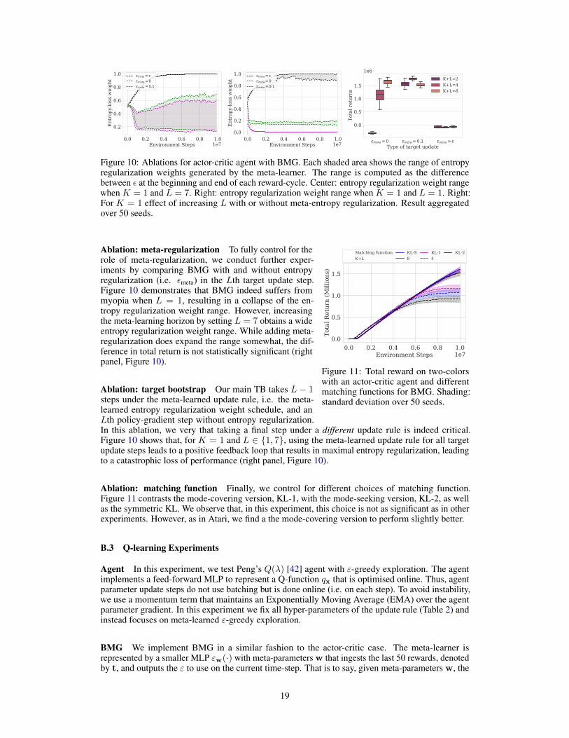
Figure 10: Ablations for actor-critic agent with BMG. Each shaded area shows the range of entropyregularization weights generated by the meta-learner. The range is computed as the differencebetween ε at the beginning and end of each reward-cycle. Center: entropy regularization weight rangewhen K = 1 and L = 7. Right: entropy regularization weight range when K = 1 and L = 1. Right:For K = 1 effect of increasing L with or without meta-entropy regularization. Result aggregatedover 50 seeds.
0.0 0.2 0.4 0.6 0.8 1.0Environment Steps 1e7
0.0
0.5
1.0
1.5
Tota
l Ret
urn
(Mill
ions
)
Matching functionK+L
KL-S8
KL-14
KL-2
Figure 11: Total reward on two-colorswith an actor-critic agent and differentmatching functions for BMG. Shading:standard deviation over 50 seeds.
Ablation: meta-regularization To fully control for therole of meta-regularization, we conduct further exper-iments by comparing BMG with and without entropyregularization (i.e. εmeta) in the Lth target update step.Figure 10 demonstrates that BMG indeed suffers frommyopia when L = 1, resulting in a collapse of the en-tropy regularization weight range. However, increasingthe meta-learning horizon by setting L = 7 obtains a wideentropy regularization weight range. While adding meta-regularization does expand the range somewhat, the dif-ference in total return is not statistically significant (rightpanel, Figure 10).
Ablation: target bootstrap Our main TB takes L − 1steps under the meta-learned update rule, i.e. the meta-learned entropy regularization weight schedule, and anLth policy-gradient step without entropy regularization.In this ablation, we very that taking a final step under a different update rule is indeed critical.Figure 10 shows that, for K = 1 and L ∈ {1, 7}, using the meta-learned update rule for all targetupdate steps leads to a positive feedback loop that results in maximal entropy regularization, leadingto a catastrophic loss of performance (right panel, Figure 10).
Ablation: matching function Finally, we control for different choices of matching function.Figure 11 contrasts the mode-covering version, KL-1, with the mode-seeking version, KL-2, as wellas the symmetric KL. We observe that, in this experiment, this choice is not as significant as in otherexperiments. However, as in Atari, we find a the mode-covering version to perform slightly better.
B.3 Q-learning Experiments
Agent In this experiment, we test Peng’s Q(λ) [42] agent with ε-greedy exploration. The agentimplements a feed-forward MLP to represent a Q-function qx that is optimised online. Thus, agentparameter update steps do not use batching but is done online (i.e. on each step). To avoid instability,we use a momentum term that maintains an Exponentially Moving Average (EMA) over the agentparameter gradient. In this experiment we fix all hyper-parameters of the update rule (Table 2) andinstead focuses on meta-learned ε-greedy exploration.
BMG We implement BMG in a similar fashion to the actor-critic case. The meta-learner isrepresented by a smaller MLP εw(·) with meta-parameters w that ingests the last 50 rewards, denotedby t, and outputs the ε to use on the current time-step. That is to say, given meta-parameters w, the
19
0.05
0.15
0.25
Rew
./Ste
p
0 100000 200000 300000Env Steps into Cycle
0.1
0.2
0.3
0.4
No MG L=16 L=32 L=128
0.00 0.25 0.50 0.75 1.00Environment Steps 1e7
0.0
0.5
1.0
1.5
Tota
l Ret
urns
(Mill
ions
)
L=16L=32L=128Fixed = 0.3
0.0 0.2 0.4 0.6 0.8 1.0Environment Steps 1e7
0.0
0.5
1.0
1.5
2.0
Tota
l Ret
urns
(Mill
ions
) Policy Matching"Value" matchingFixed = 0.3
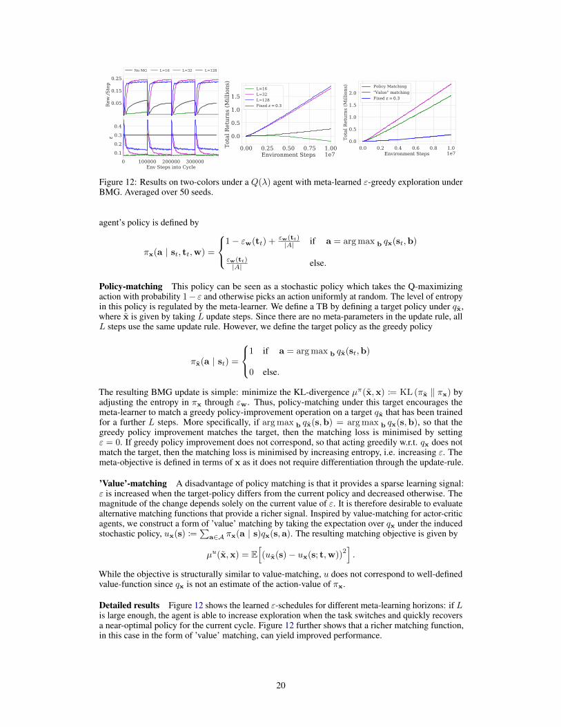
Figure 12: Results on two-colors under a Q(λ) agent with meta-learned ε-greedy exploration underBMG. Averaged over 50 seeds.
agent’s policy is defined by
πx(a | st, tt,w) =
1− εw(tt) + εw(tt)|A| if a = arg max b qx(st,b)
εw(tt)|A| else.
Policy-matching This policy can be seen as a stochastic policy which takes the Q-maximizingaction with probability 1− ε and otherwise picks an action uniformly at random. The level of entropyin this policy is regulated by the meta-learner. We define a TB by defining a target policy under qx,where x is given by taking L update steps. Since there are no meta-parameters in the update rule, allL steps use the same update rule. However, we define the target policy as the greedy policy
πx(a | st) =
1 if a = arg max b qx(st,b)
0 else.
The resulting BMG update is simple: minimize the KL-divergence µπ(x,x) := KL (πx ‖ πx) byadjusting the entropy in πx through εw. Thus, policy-matching under this target encourages themeta-learner to match a greedy policy-improvement operation on a target qx that has been trainedfor a further L steps. More specifically, if arg max b qx(s,b) = arg max b qx(s,b), so that thegreedy policy improvement matches the target, then the matching loss is minimised by settingε = 0. If greedy policy improvement does not correspond, so that acting greedily w.r.t. qx does notmatch the target, then the matching loss is minimised by increasing entropy, i.e. increasing ε. Themeta-objective is defined in terms of x as it does not require differentiation through the update-rule.
’Value’-matching A disadvantage of policy matching is that it provides a sparse learning signal:ε is increased when the target-policy differs from the current policy and decreased otherwise. Themagnitude of the change depends solely on the current value of ε. It is therefore desirable to evaluatealternative matching functions that provide a richer signal. Inspired by value-matching for actor-criticagents, we construct a form of ’value’ matching by taking the expectation over qx under the inducedstochastic policy, ux(s) :=
∑a∈A πx(a | s)qx(s,a). The resulting matching objective is given by
µu(x,x) = E[(ux(s)− ux(s; t,w))
2].
While the objective is structurally similar to value-matching, u does not correspond to well-definedvalue-function since qx is not an estimate of the action-value of πx.
Detailed results Figure 12 shows the learned ε-schedules for different meta-learning horizons: if Lis large enough, the agent is able to increase exploration when the task switches and quickly recoversa near-optimal policy for the current cycle. Figure 12 further shows that a richer matching function,in this case in the form of ’value’ matching, can yield improved performance.
20
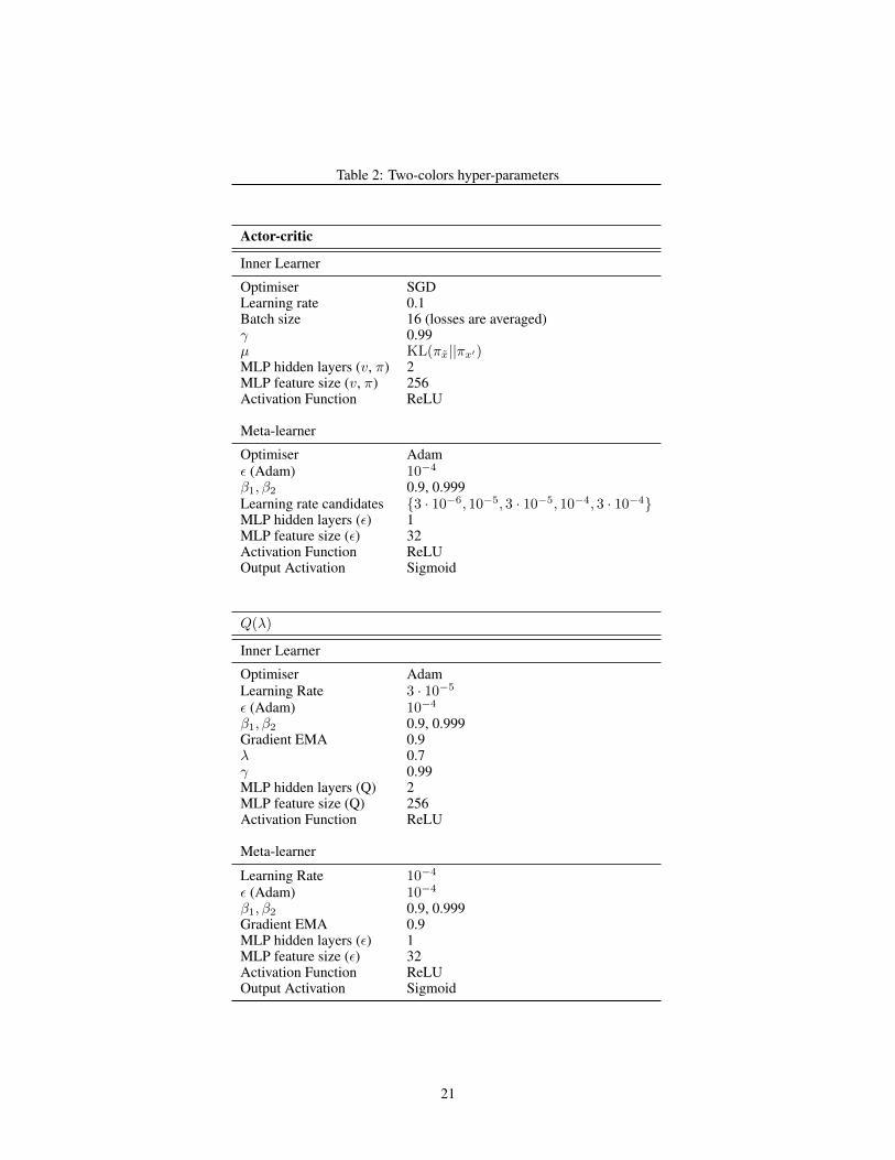
Table 2: Two-colors hyper-parameters
Actor-critic
Inner Learner
Optimiser SGDLearning rate 0.1Batch size 16 (losses are averaged)γ 0.99µ KL(πx||πx′)MLP hidden layers (v, π) 2MLP feature size (v, π) 256Activation Function ReLU
Meta-learner
Optimiser Adamε (Adam) 10−4
β1, β2 0.9, 0.999Learning rate candidates {3 · 10−6, 10−5, 3 · 10−5, 10−4, 3 · 10−4}MLP hidden layers (ε) 1MLP feature size (ε) 32Activation Function ReLUOutput Activation Sigmoid
Q(λ)
Inner Learner
Optimiser AdamLearning Rate 3 · 10−5
ε (Adam) 10−4
β1, β2 0.9, 0.999Gradient EMA 0.9λ 0.7γ 0.99MLP hidden layers (Q) 2MLP feature size (Q) 256Activation Function ReLU
Meta-learner
Learning Rate 10−4
ε (Adam) 10−4
β1, β2 0.9, 0.999Gradient EMA 0.9MLP hidden layers (ε) 1MLP feature size (ε) 32Activation Function ReLUOutput Activation Sigmoid
21
C AtariTable 3: Atari hyper-parameters
ALE [8]
Frame dimensions (H, W, D) 160, 210, 3Frame pooling NoneFrame grayscaling NoneNum. stacked frames 4Num. action repeats 4Sticky actions [33] FalseReward clipping [−1, 1]γ = 0 loss of life TrueMax episode length 108 000 framesInitial noop actions 30
IMPALA Network [15]
Convolutional layers 4Channel depths 64, 128, 128, 64Kernel size 3Kernel stride 1Pool size 3Pool stride 2Padding ’SAME’Residual blocks per layer 2Conv-to-linear feature size 512
STACX [68]
Auxiliary tasks 2MLP hidden layers 2MLP feature size 256Max entropy loss value 0.9
Optimisation
Unroll length 20Batch size 18
of which from replay 12of which is online data 6
Replay buffer size 10 000LASER [49] KL-threshold 2Optimiser RMSPropInitial learning rate 10−4
Learning rate decay interval 200 000 framesLearning rate decay rate Linear to 0Momentum decay 0.99Epsilon 10−4
Gradient clipping, max norm 0.3
Meta-Optimisation
γ, λ, ρ, c, α 0.995, 1, 1, 1, 1εPG, εEN, εTD 1, 0.01, 0.25Optimiser AdamLearning rate 10−3
β1, β2 0.9, 0.999Epsilon 10−4
Gradient clipping, max norm 0.3
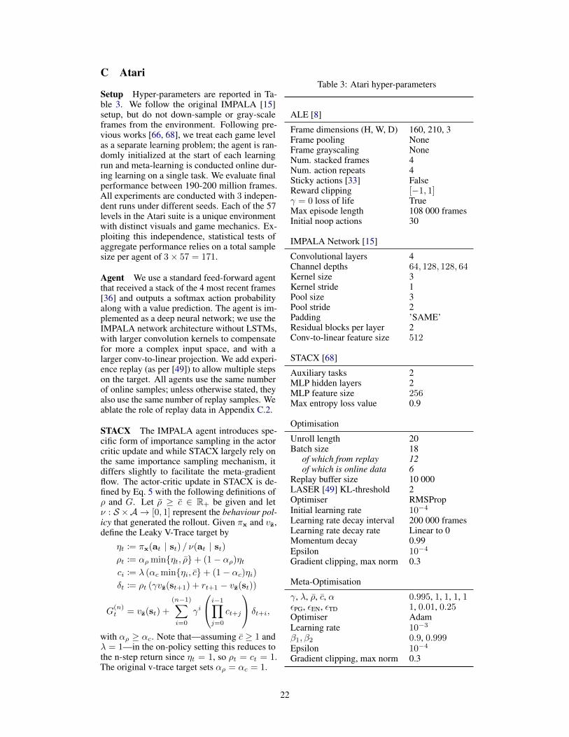
Setup Hyper-parameters are reported in Ta-ble 3. We follow the original IMPALA [15]setup, but do not down-sample or gray-scaleframes from the environment. Following pre-vious works [66, 68], we treat each game levelas a separate learning problem; the agent is ran-domly initialized at the start of each learningrun and meta-learning is conducted online dur-ing learning on a single task. We evaluate finalperformance between 190-200 million frames.All experiments are conducted with 3 indepen-dent runs under different seeds. Each of the 57levels in the Atari suite is a unique environmentwith distinct visuals and game mechanics. Ex-ploiting this independence, statistical tests ofaggregate performance relies on a total samplesize per agent of 3× 57 = 171.
Agent We use a standard feed-forward agentthat received a stack of the 4 most recent frames[36] and outputs a softmax action probabilityalong with a value prediction. The agent is im-plemented as a deep neural network; we use theIMPALA network architecture without LSTMs,with larger convolution kernels to compensatefor more a complex input space, and with alarger conv-to-linear projection. We add experi-ence replay (as per [49]) to allow multiple stepson the target. All agents use the same numberof online samples; unless otherwise stated, theyalso use the same number of replay samples. Weablate the role of replay data in Appendix C.2.
STACX The IMPALA agent introduces spe-cific form of importance sampling in the actorcritic update and while STACX largely rely onthe same importance sampling mechanism, itdiffers slightly to facilitate the meta-gradientflow. The actor-critic update in STACX is de-fined by Eq. 5 with the following definitions ofρ and G. Let ρ ≥ c ∈ R+ be given and letν : S ×A → [0, 1] represent the behaviour pol-icy that generated the rollout. Given πx and vz,define the Leaky V-Trace target by
ηt := πx(at | st) / ν(at | st)ρt := αρ min{ηt, ρ}+ (1− αρ)ηtci := λ (αc min{ηi, c}+ (1− αc)ηi)δt := ρt (γvz(st+1) + rt+1 − vz(st))
G(n)t = vz(st) +
(n−1)∑i=0
γi
i−1∏j=0
ct+j
δt+i,
with αρ ≥ αc. Note that—assuming c ≥ 1 andλ = 1—in the on-policy setting this reduces tothe n-step return since ηt = 1, so ρt = ct = 1.The original v-trace target sets αρ = αc = 1.
22
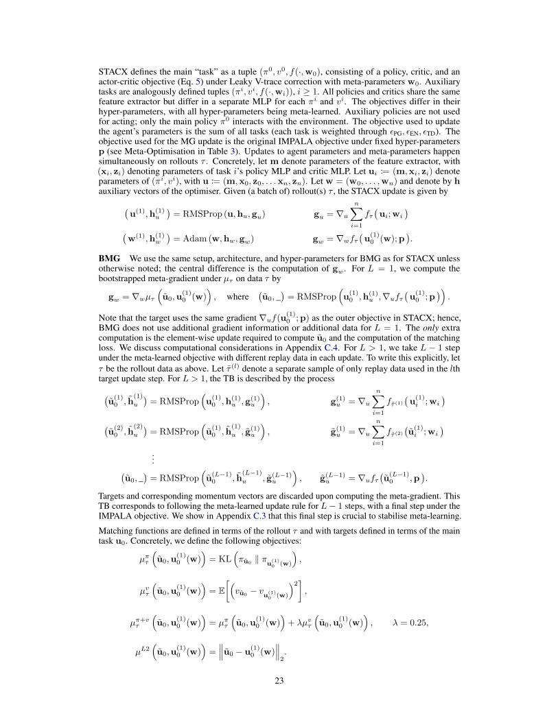
STACX defines the main “task” as a tuple (π0, v0, f(·,w0), consisting of a policy, critic, and anactor-critic objective (Eq. 5) under Leaky V-trace correction with meta-parameters w0. Auxiliarytasks are analogously defined tuples (πi, vi, f(·,wi)), i ≥ 1. All policies and critics share the samefeature extractor but differ in a separate MLP for each πi and vi. The objectives differ in theirhyper-parameters, with all hyper-parameters being meta-learned. Auxiliary policies are not usedfor acting; only the main policy π0 interacts with the environment. The objective used to updatethe agent’s parameters is the sum of all tasks (each task is weighted through εPG, εEN, εTD). Theobjective used for the MG update is the original IMPALA objective under fixed hyper-parametersp (see Meta-Optimisation in Table 3). Updates to agent parameters and meta-parameters happensimultaneously on rollouts τ . Concretely, let m denote parameters of the feature extractor, with(xi, zi) denoting parameters of task i’s policy MLP and critic MLP. Let ui := (m,xi, zi) denoteparameters of (πi, vi), with u := (m,x0, z0, . . .xn, zn). Let w = (w0, . . . ,wn) and denote by hauxiliary vectors of the optimiser. Given (a batch of) rollout(s) τ , the STACX update is given by(
u(1),h(1)u
)= RMSProp (u,hu,gu) gu = ∇u
n∑i=1
fτ(ui;wi
)(w(1),h(1)
w
)= Adam (w,hw,gw) gw = ∇wfτ
(u
(1)0 (w);p
).
BMG We use the same setup, architecture, and hyper-parameters for BMG as for STACX unlessotherwise noted; the central difference is the computation of gw. For L = 1, we compute thebootstrapped meta-gradient under µτ on data τ by
gw = ∇wµτ(u0,u
(1)0 (w)
), where
(u0, _
)= RMSProp
(u
(1)0 ,h(1)
u ,∇ufτ(u
(1)0 ;p
)).
Note that the target uses the same gradient ∇uf(u(1)0 ;p) as the outer objective in STACX; hence,
BMG does not use additional gradient information or additional data for L = 1. The only extracomputation is the element-wise update required to compute u0 and the computation of the matchingloss. We discuss computational considerations in Appendix C.4. For L > 1, we take L − 1 stepunder the meta-learned objective with different replay data in each update. To write this explicitly, letτ be the rollout data as above. Let τ (l) denote a separate sample of only replay data used in the lthtarget update step. For L > 1, the TB is described by the process(
u(1)0 , h
(1)
u
)= RMSProp
(u
(1)0 ,h(1)
u ,g(1)u
), g(1)
u = ∇un∑i=1
fτ(1)
(u
(1)i ;wi
)(u
(2)0 , h
(2)
u
)= RMSProp
(u
(1)0 , h
(1)
u , g(1)u
), g(1)
u = ∇un∑i=1
fτ(2)
(u
(1)i ;wi
)...(
u0, _)
= RMSProp(u
(L−1)0 , h
(L−1)
u , g(L−1)u
), g(L−1)
u = ∇ufτ(u
(L−1)0 ,p
).
Targets and corresponding momentum vectors are discarded upon computing the meta-gradient. ThisTB corresponds to following the meta-learned update rule for L− 1 steps, with a final step under theIMPALA objective. We show in Appendix C.3 that this final step is crucial to stabilise meta-learning.
Matching functions are defined in terms of the rollout τ and with targets defined in terms of the maintask u0. Concretely, we define the following objectives:
µπτ
(u0,u
(1)0 (w)
)= KL
(πu0‖ π
u(1)0 (w)
),
µvτ
(u0,u
(1)0 (w)
)= E
[(vu0− v
u(1)0 (w)
)2],
µπ+vτ
(u0,u
(1)0 (w)
)= µπτ
(u0,u
(1)0 (w)
)+ λµvτ
(u0,u
(1)0 (w)
), λ = 0.25,
µL2(u0,u
(1)0 (w)
)=∥∥∥u0 − u
(1)0 (w)
∥∥∥2.
23
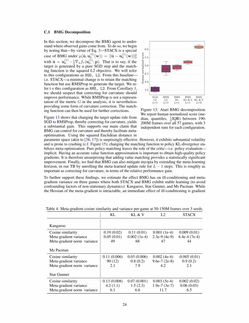
C.1 BMG Decomposition
SGDL2
L=1
RMSL2
L=1
RMSKL
L=1
RMSKL & V
L=1
RMSKL & V
L=4
3.5
4.0
4.5
5.0
5.5
6.0
Hum
an n
orm
aliz
ed s
core
Figure 13: Atari BMG decomposition.We report human normalized score (me-dian, quantiles, 1
2 IQR) between 190-200M frames over all 57 games, with 3independent runs for each configuration.
In this section, we decompose the BMG agent to under-stand where observed gains come from. To do so, we beginby noting that—by virtue of Eq. 3—STACX is a specialcase of BMG under µ(u,u
(1)0 (w)) = ‖u − u
(1)0 (w)‖22
with u = u(1)0 − 1
2∇ufτ (u(1)0 ;p). That is to say, if the
target is generated by a pure SGD step and the match-ing function is the squared L2 objective. We will referto this configurations as SGD, L2. From this baseline—i.e. STACX—a minimal change is to retain the matchingfunction but use RMSProp to generate the target. We re-fer t o this configuration as RMS, L2. From Corollary 1,we should suspect that correcting for curvature shouldimprove performance. While RMSProp is not a represen-tation of the metric G in the analysis, it is neverthelessproviding some form of curvature correction. The match-ing function can then be used for further corrections.
Figure 13 shows that changing the target update rule fromSGD to RMSProp, thereby correcting for curvature, yieldsa substantial gain. This supports our main claim thatBMG can control for curvature and thereby facilitate meta-optimisation. Using the squared Euclidean distance inparameter space (akin to [38, 17]) is surprisingly effective. However, it exhibits substantial volatilityand is prone to crashing (c.f. Figure 15); changing the matching function to policy KL-divergence sta-bilizes meta-optimisation. Pure policy-matching leaves the role of the critic—i.e. policy evaluation—implicit. Having an accurate value function approximation is important to obtain high-quality policygradients. It is therefore unsurprising that adding value matching provides a statistically significantimprovement. Finally, we find that BMG can also mitigate myopia by extending the meta-learninghorizon, in our TB by unrolling the meta-learned update rule for L − 1 steps. This is roughly asimportant as correcting for curvature, in terms of the relative performance gain.
To further support these findings, we estimate the effect BMG has on ill-conditioning and meta-gradient variance on three games where both STACX and BMG exhibit stable learning (to avoidconfounding factors of non-stationary dynamics): Kangaroo, Star Gunner, and Ms Pacman. Whilethe Hessian of the meta-gradient is intractable, an immediate effect of ill-conditioning is gradient
Table 4: Meta-gradient cosine similarity and variance per-game at 50-150M frames over 3 seeds.KL KL & V L2 STACX
Kangaroo
Cosine similarity 0.19 (0.02) 0.11 (0.01) 0.001 (1e-4) 0.009 (0.01)Meta-gradient variance 0.05 (0.01) 0.002 (1e-4) 2.3e-9 (4e-9) 6.4e-4 (7e-4)Meta-gradient norm variance 49 68 47 44
Ms Pacman
Cosine similarity 0.11 (0.006) 0.03 (0.006) 0.002 (4e-4) -0.005 (0.01)Meta-gradient variance 90 (12) 0.8 (0.2) 9.6e-7 (2e-8) 0.9 (0.2)Meta-gradient norm variance 2.1 7.9 4.2 2.1
Star Gunner
Cosine similarity 0.13 (0.008) 0.07 (0.001) 0.003 (5e-4) 0.002 (0.02)Meta-gradient variance 4.2 (1.1) 1.5 (2.3) 1.9e-7 (3e-7) 0.06 (0.03)Meta-gradient norm variance 6.1 6.6 11.7 6.5
24
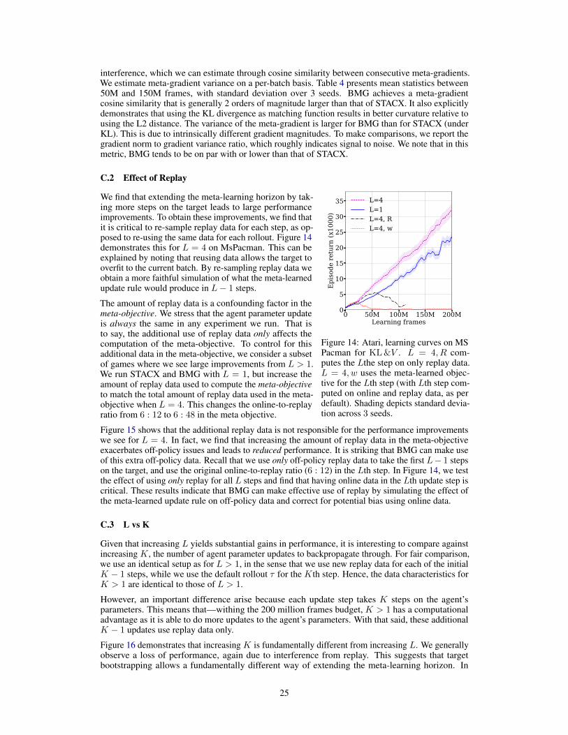
interference, which we can estimate through cosine similarity between consecutive meta-gradients.We estimate meta-gradient variance on a per-batch basis. Table 4 presents mean statistics between50M and 150M frames, with standard deviation over 3 seeds. BMG achieves a meta-gradientcosine similarity that is generally 2 orders of magnitude larger than that of STACX. It also explicitlydemonstrates that using the KL divergence as matching function results in better curvature relative tousing the L2 distance. The variance of the meta-gradient is larger for BMG than for STACX (underKL). This is due to intrinsically different gradient magnitudes. To make comparisons, we report thegradient norm to gradient variance ratio, which roughly indicates signal to noise. We note that in thismetric, BMG tends to be on par with or lower than that of STACX.
C.2 Effect of Replay
0 50M 100M 150M 200MLearning frames
0
5
10
15
20
25
30
35
Epi
sode
ret
urn
(x10
00)
L=4L=1L=4, RL=4, w
Figure 14: Atari, learning curves on MSPacman for KL &V . L = 4, R com-putes the Lthe step on only replay data.L = 4, w uses the meta-learned objec-tive for the Lth step (with Lth step com-puted on online and replay data, as perdefault). Shading depicts standard devia-tion across 3 seeds.
We find that extending the meta-learning horizon by tak-ing more steps on the target leads to large performanceimprovements. To obtain these improvements, we find thatit is critical to re-sample replay data for each step, as op-posed to re-using the same data for each rollout. Figure 14demonstrates this for L = 4 on MsPacman. This can beexplained by noting that reusing data allows the target tooverfit to the current batch. By re-sampling replay data weobtain a more faithful simulation of what the meta-learnedupdate rule would produce in L− 1 steps.
The amount of replay data is a confounding factor in themeta-objective. We stress that the agent parameter updateis always the same in any experiment we run. That isto say, the additional use of replay data only affects thecomputation of the meta-objective. To control for thisadditional data in the meta-objective, we consider a subsetof games where we see large improvements from L > 1.We run STACX and BMG with L = 1, but increase theamount of replay data used to compute the meta-objectiveto match the total amount of replay data used in the meta-objective when L = 4. This changes the online-to-replayratio from 6 : 12 to 6 : 48 in the meta objective.
Figure 15 shows that the additional replay data is not responsible for the performance improvementswe see for L = 4. In fact, we find that increasing the amount of replay data in the meta-objectiveexacerbates off-policy issues and leads to reduced performance. It is striking that BMG can make useof this extra off-policy data. Recall that we use only off-policy replay data to take the first L− 1 stepson the target, and use the original online-to-replay ratio (6 : 12) in the Lth step. In Figure 14, we testthe effect of using only replay for all L steps and find that having online data in the Lth update step iscritical. These results indicate that BMG can make effective use of replay by simulating the effect ofthe meta-learned update rule on off-policy data and correct for potential bias using online data.
C.3 L vs K
Given that increasing L yields substantial gains in performance, it is interesting to compare againstincreasing K, the number of agent parameter updates to backpropagate through. For fair comparison,we use an identical setup as for L > 1, in the sense that we use new replay data for each of the initialK − 1 steps, while we use the default rollout τ for the Kth step. Hence, the data characteristics forK > 1 are identical to those of L > 1.
However, an important difference arise because each update step takes K steps on the agent’sparameters. This means that—withing the 200 million frames budget, K > 1 has a computationaladvantage as it is able to do more updates to the agent’s parameters. With that said, these additionalK − 1 updates use replay data only.
Figure 16 demonstrates that increasing K is fundamentally different from increasing L. We generallyobserve a loss of performance, again due to interference from replay. This suggests that targetbootstrapping allows a fundamentally different way of extending the meta-learning horizon. In
25
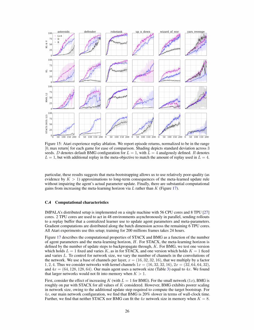
0
25
50
75
100
KL
& V
asteroidsL=4DR
defender robotank up_n_down wizard_of_wor yars_revenge
0
25
50
75
100
KL
0
25
50
75
100
RM
S, L
2
0 50 100 150 2000
25
50
75
100
STAC
X (S
GD
, L2)
0 50 100 150 200 0 50 100 150 200 0 50 100 150 200 0 50 100 150 200 0 50 100 150 200
Figure 15: Atari experience replay ablation. We report episode returns, normalized to be in the range[0,max return] for each game for ease of comparison. Shading depicts standard deviation across 3seeds. D denotes default BMG configuration for L = 1, with L = 4 analgously defined. R denotesL = 1, but with additional replay in the meta-objective to match the amount of replay used in L = 4.
particular, these results suggests that meta-bootstrapping allows us to use relatively poor-quality (asevidence by K > 1) approximations to long-term consequences of the meta-learned update rulewithout impairing the agent’s actual parameter update. Finally, there are substantial computationalgains from increasing the meta-learning horizon via L rather than K (Figure 17).
C.4 Computational characteristics
IMPALA’s distributed setup is implemented on a single machine with 56 CPU cores and 8 TPU [27]cores. 2 TPU cores are used to act in 48 environments asynchronously in parallel, sending rolloutsto a replay buffer that a centralized learner use to update agent parameters and meta-parameters.Gradient computations are distributed along the batch dimension across the remaining 6 TPU cores.All Atari experiments use this setup; training for 200 millions frames takes 24 hours.
Figure 17 describes the computational properties of STACX and BMG as a function of the numberof agent parameters and the meta-learning horizon, H . For STACX, the meta-learning horizon isdefined by the number of update steps to backpropagate through, K. For BMG, we test one versionwhich holds L = 1 fixed and varies K, as in for STACX, and one version which holds K = 1 ficedand varies L. To control for network size, we vary the number of channels in the convolutions ofthe network. We use a base of channels per layer, x = (16, 32, 32, 16), that we multiply by a factor1, 2, 4. Thus we consider networks with kernel channels 1x = (16, 32, 32, 16), 2x = (32, 64, 64, 32),and 4x = (64, 128, 128, 64). Our main agent uses a network size (Table 3) equal to 4x. We foundthat larger networks would not fit into memory when K > 1.
First, consider the effect of increasing K (with L = 1 for BMG). For the small network (1x), BMG isroughly on par with STACX for all values of K considered. However, BMG exhibits poorer scalingin network size, owing to the additional update step required to compute the target bootstrap. For4x, our main network configuration, we find that BMG is 20% slower in terms of wall-clock time.Further, we find that neither STACX nor BMG can fit the 4x network size in memory when K = 8.
26
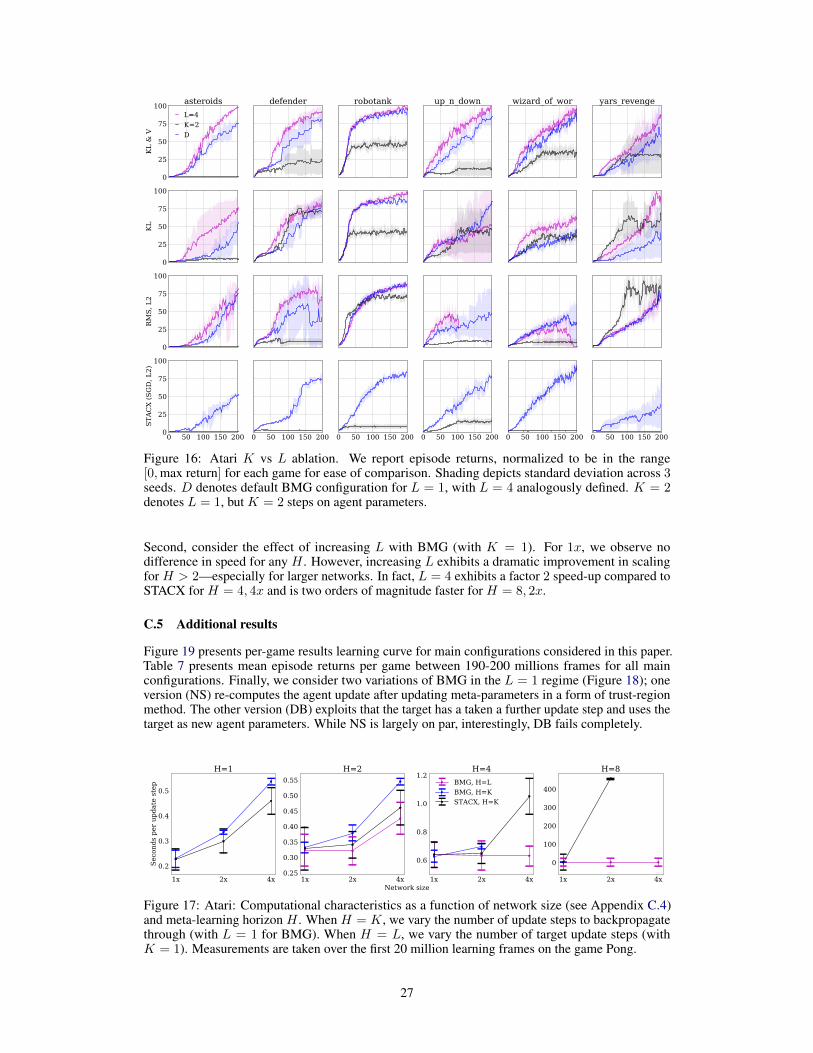
0
25
50
75
100
KL
& V
asteroidsL=4K=2D
defender robotank up_n_down wizard_of_wor yars_revenge
0
25
50
75
100
KL
0
25
50
75
100
RM
S, L
2
0 50 100 150 2000
25
50
75
100
STAC
X (S
GD
, L2)
0 50 100 150 200 0 50 100 150 200 0 50 100 150 200 0 50 100 150 200 0 50 100 150 200
Figure 16: Atari K vs L ablation. We report episode returns, normalized to be in the range[0,max return] for each game for ease of comparison. Shading depicts standard deviation across 3seeds. D denotes default BMG configuration for L = 1, with L = 4 analogously defined. K = 2denotes L = 1, but K = 2 steps on agent parameters.
Second, consider the effect of increasing L with BMG (with K = 1). For 1x, we observe nodifference in speed for any H . However, increasing L exhibits a dramatic improvement in scalingfor H > 2—especially for larger networks. In fact, L = 4 exhibits a factor 2 speed-up compared toSTACX for H = 4, 4x and is two orders of magnitude faster for H = 8, 2x.
C.5 Additional results
Figure 19 presents per-game results learning curve for main configurations considered in this paper.Table 7 presents mean episode returns per game between 190-200 millions frames for all mainconfigurations. Finally, we consider two variations of BMG in the L = 1 regime (Figure 18); oneversion (NS) re-computes the agent update after updating meta-parameters in a form of trust-regionmethod. The other version (DB) exploits that the target has a taken a further update step and uses thetarget as new agent parameters. While NS is largely on par, interestingly, DB fails completely.
1x 2x 4x
0.2
0.3
0.4
0.5
Seco
nds
per
upda
te s
tep
H=1
1x 2x 4x0.25
0.30
0.35
0.40
0.45
0.50
0.55H=2
1x 2x 4x
0.6
0.8
1.0
1.2H=4
BMG, H=LBMG, H=KSTACX, H=K
1x 2x 4x
0
100
200
300
400
H=8
Network size
Figure 17: Atari: Computational characteristics as a function of network size (see Appendix C.4)and meta-learning horizon H . When H = K, we vary the number of update steps to backpropagatethrough (with L = 1 for BMG). When H = L, we vary the number of target update steps (withK = 1). Measurements are taken over the first 20 million learning frames on the game Pong.
27
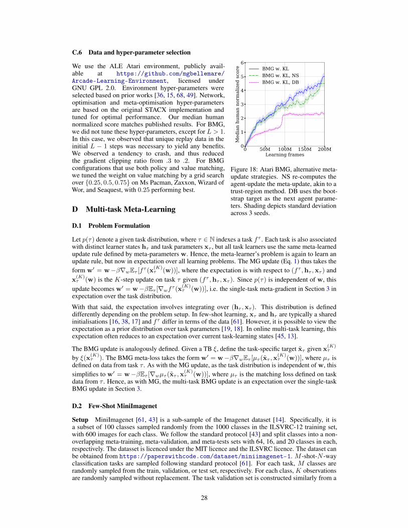
C.6 Data and hyper-parameter selection
0 50M 100M 150M 200MLearning frames
0
1
2
3
4
5
6
Med
ian
hum
an n
orm
aliz
ed s
core BMG w. KL
BMG w. KL, NSBMG w. KL, DB
Figure 18: Atari BMG, alternative meta-update strategies. NS re-computes theagent-update the meta-update, akin to atrust-region method. DB uses the boot-strap target as the next agent parame-ters. Shading depicts standard deviationacross 3 seeds.
We use the ALE Atari environment, publicly avail-able at https://github.com/mgbellemare/Arcade-Learning-Environment, licensed underGNU GPL 2.0. Environment hyper-parameters wereselected based on prior works [36, 15, 68, 49]. Network,optimisation and meta-optimisation hyper-parametersare based on the original STACX implementation andtuned for optimal performance. Our median humannormalized score matches published results. For BMG,we did not tune these hyper-parameters, except for L > 1.In this case, we observed that unique replay data in theinitial L − 1 steps was necessary to yield any benefits.We observed a tendency to crash, and thus reducedthe gradient clipping ratio from .3 to .2. For BMGconfigurations that use both policy and value matching,we tuned the weight on value matching by a grid searchover {0.25, 0.5, 0.75} on Ms Pacman, Zaxxon, Wizard ofWor, and Seaquest, with 0.25 performing best.
D Multi-task Meta-Learning
D.1 Problem Formulation
Let p(τ) denote a given task distribution, where τ ∈ N indexes a task fτ . Each task is also associatedwith distinct learner states hτ and task parameters xτ , but all task learners use the same meta-learnedupdate rule defined by meta-parameters w. Hence, the meta-learner’s problem is again to learn anupdate rule, but now in expectation over all learning problems. The MG update (Eq. 1) thus takes theform w′ = w−β∇wEτ [fτ (x
(K)τ (w))], where the expectation is with respect to (fτ ,hτ ,xτ ) and
x(K)τ (w) is the K-step update on task τ given (fτ ,hτ ,xτ ). Since p(τ) is independent of w, this
update becomes w′ = w−βEτ [∇wfτ (x(K)τ (w))], i.e. the single-task meta-gradient in Section 3 in
expectation over the task distribution.
With that said, the expectation involves integrating over (hτ ,xτ ). This distribution is defineddifferently depending on the problem setup. In few-shot learning, xτ and hτ are typically a sharedinitialisations [16, 38, 17] and fτ differ in terms of the data [61]. However, it is possible to view theexpectation as a prior distribution over task parameters [19, 18]. In online multi-task learning, thisexpectation often reduces to an expectation over current task-learning states [45, 13].
The BMG update is analogously defined. Given a TB ξ, define the task-specific target xτ given x(K)τ
by ξ(x(K)τ ). The BMG meta-loss takes the form w′ = w−β∇wEτ [µτ (xτ ,x
(K)τ (w))], where µτ is
defined on data from task τ . As with the MG update, as the task distribution is independent of w, thissimplifies to w′ = w−βEτ [∇wµτ (xτ ,x
(K)τ (w))], where µτ is the matching loss defined on task
data from τ . Hence, as with MG, the multi-task BMG update is an expectation over the single-taskBMG update in Section 3.
D.2 Few-Shot MiniImagenet
Setup MiniImagenet [61, 43] is a sub-sample of the Imagenet dataset [14]. Specifically, it isa subset of 100 classes sampled randomly from the 1000 classes in the ILSVRC-12 training set,with 600 images for each class. We follow the standard protocol [43] and split classes into a non-overlapping meta-training, meta-validation, and meta-tests sets with 64, 16, and 20 classes in each,respectively. The datasset is licenced under the MIT licence and the ILSVRC licence. The dataset canbe obtained from https://paperswithcode.com/dataset/miniimagenet-1. M -shot-N -wayclassification tasks are sampled following standard protocol [61]. For each task, M classes arerandomly sampled from the train, validation, or test set, respectively. For each class, K observationsare randomly sampled without replacement. The task validation set is constructed similarly from a
28
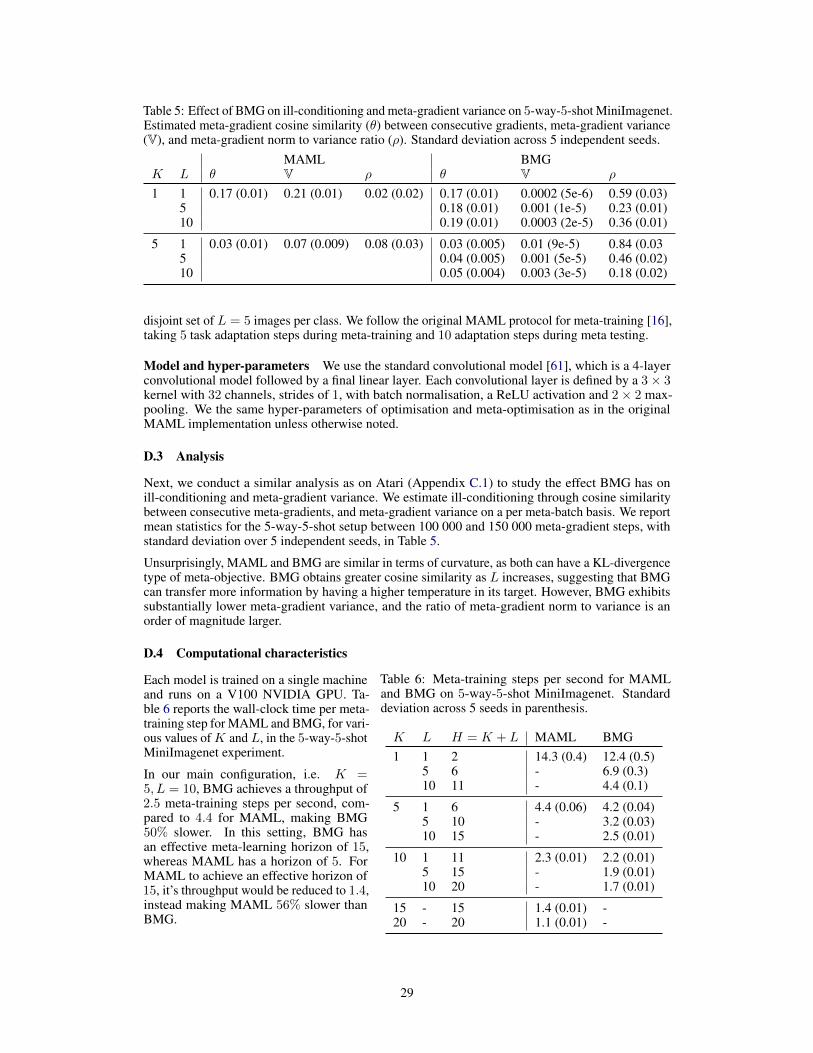
Table 5: Effect of BMG on ill-conditioning and meta-gradient variance on 5-way-5-shot MiniImagenet.Estimated meta-gradient cosine similarity (θ) between consecutive gradients, meta-gradient variance(V), and meta-gradient norm to variance ratio (ρ). Standard deviation across 5 independent seeds.
MAML BMGK L θ V ρ θ V ρ
1 1 0.17 (0.01) 0.21 (0.01) 0.02 (0.02) 0.17 (0.01) 0.0002 (5e-6) 0.59 (0.03)5 0.18 (0.01) 0.001 (1e-5) 0.23 (0.01)10 0.19 (0.01) 0.0003 (2e-5) 0.36 (0.01)
5 1 0.03 (0.01) 0.07 (0.009) 0.08 (0.03) 0.03 (0.005) 0.01 (9e-5) 0.84 (0.035 0.04 (0.005) 0.001 (5e-5) 0.46 (0.02)10 0.05 (0.004) 0.003 (3e-5) 0.18 (0.02)
disjoint set of L = 5 images per class. We follow the original MAML protocol for meta-training [16],taking 5 task adaptation steps during meta-training and 10 adaptation steps during meta testing.
Model and hyper-parameters We use the standard convolutional model [61], which is a 4-layerconvolutional model followed by a final linear layer. Each convolutional layer is defined by a 3× 3kernel with 32 channels, strides of 1, with batch normalisation, a ReLU activation and 2× 2 max-pooling. We the same hyper-parameters of optimisation and meta-optimisation as in the originalMAML implementation unless otherwise noted.
D.3 Analysis
Next, we conduct a similar analysis as on Atari (Appendix C.1) to study the effect BMG has onill-conditioning and meta-gradient variance. We estimate ill-conditioning through cosine similaritybetween consecutive meta-gradients, and meta-gradient variance on a per meta-batch basis. We reportmean statistics for the 5-way-5-shot setup between 100 000 and 150 000 meta-gradient steps, withstandard deviation over 5 independent seeds, in Table 5.
Unsurprisingly, MAML and BMG are similar in terms of curvature, as both can have a KL-divergencetype of meta-objective. BMG obtains greater cosine similarity as L increases, suggesting that BMGcan transfer more information by having a higher temperature in its target. However, BMG exhibitssubstantially lower meta-gradient variance, and the ratio of meta-gradient norm to variance is anorder of magnitude larger.
D.4 Computational characteristics
Table 6: Meta-training steps per second for MAMLand BMG on 5-way-5-shot MiniImagenet. Standarddeviation across 5 seeds in parenthesis.
K L H = K + L MAML BMG1 1 2 14.3 (0.4) 12.4 (0.5)
5 6 - 6.9 (0.3)10 11 - 4.4 (0.1)
5 1 6 4.4 (0.06) 4.2 (0.04)5 10 - 3.2 (0.03)10 15 - 2.5 (0.01)
10 1 11 2.3 (0.01) 2.2 (0.01)5 15 - 1.9 (0.01)10 20 - 1.7 (0.01)
15 - 15 1.4 (0.01) -20 - 20 1.1 (0.01) -
Each model is trained on a single machineand runs on a V100 NVIDIA GPU. Ta-ble 6 reports the wall-clock time per meta-training step for MAML and BMG, for vari-ous values ofK and L, in the 5-way-5-shotMiniImagenet experiment.
In our main configuration, i.e. K =5, L = 10, BMG achieves a throughput of2.5 meta-training steps per second, com-pared to 4.4 for MAML, making BMG50% slower. In this setting, BMG hasan effective meta-learning horizon of 15,whereas MAML has a horizon of 5. ForMAML to achieve an effective horizon of15, it’s throughput would be reduced to 1.4,instead making MAML 56% slower thanBMG.
29
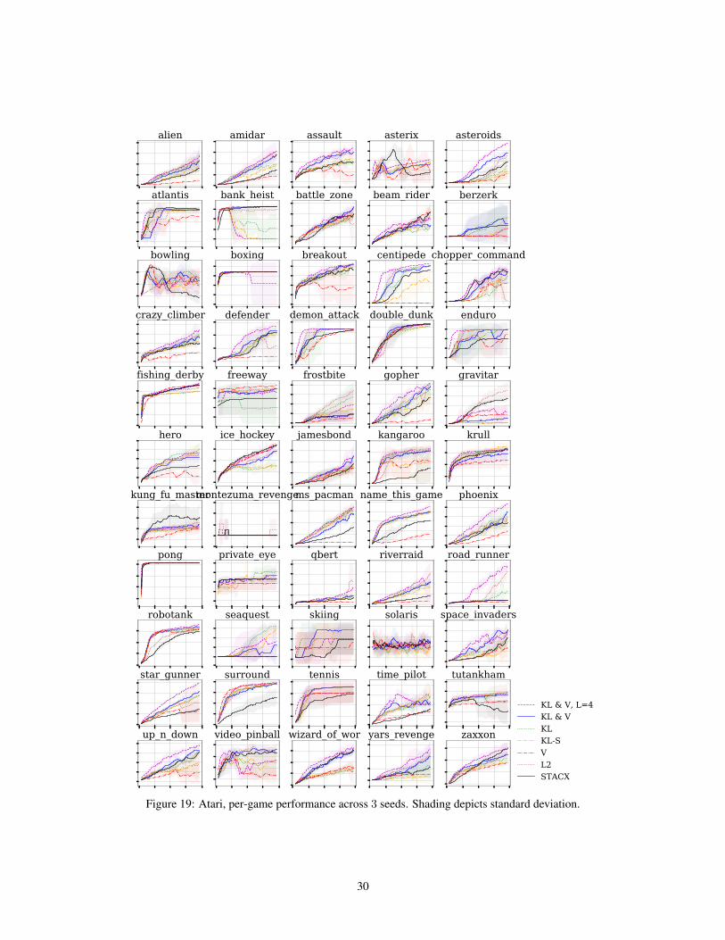
alien amidar assault asterix asteroids
atlantis bank_heist battle_zone beam_rider berzerk
bowling boxing breakout centipede chopper_command
crazy_climber defender demon_attack double_dunk enduro
fishing_derby freeway frostbite gopher gravitar
hero ice_hockey jamesbond kangaroo krull
kung_fu_mastermontezuma_revengems_pacman name_this_game phoenix
pong private_eye qbert riverraid road_runner
robotank seaquest skiing solaris space_invaders
star_gunner surround tennis time_pilot tutankham
up_n_down video_pinball wizard_of_wor yars_revenge zaxxon
KL & V, L=4KL & VKLKL-SVL2STACX
Figure 19: Atari, per-game performance across 3 seeds. Shading depicts standard deviation.
30
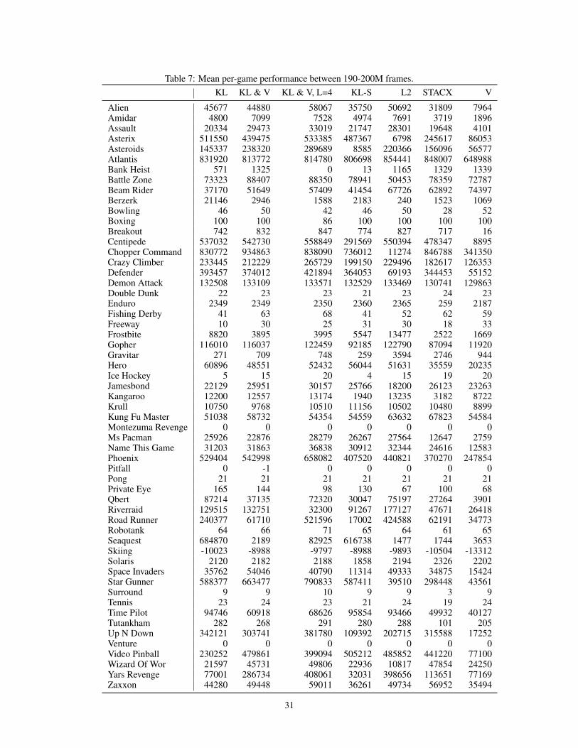
Table 7: Mean per-game performance between 190-200M frames.KL KL & V KL & V, L=4 KL-S L2 STACX V
Alien 45677 44880 58067 35750 50692 31809 7964Amidar 4800 7099 7528 4974 7691 3719 1896Assault 20334 29473 33019 21747 28301 19648 4101Asterix 511550 439475 533385 487367 6798 245617 86053Asteroids 145337 238320 289689 8585 220366 156096 56577Atlantis 831920 813772 814780 806698 854441 848007 648988Bank Heist 571 1325 0 13 1165 1329 1339Battle Zone 73323 88407 88350 78941 50453 78359 72787Beam Rider 37170 51649 57409 41454 67726 62892 74397Berzerk 21146 2946 1588 2183 240 1523 1069Bowling 46 50 42 46 50 28 52Boxing 100 100 86 100 100 100 100Breakout 742 832 847 774 827 717 16Centipede 537032 542730 558849 291569 550394 478347 8895Chopper Command 830772 934863 838090 736012 11274 846788 341350Crazy Climber 233445 212229 265729 199150 229496 182617 126353Defender 393457 374012 421894 364053 69193 344453 55152Demon Attack 132508 133109 133571 132529 133469 130741 129863Double Dunk 22 23 23 21 23 24 23Enduro 2349 2349 2350 2360 2365 259 2187Fishing Derby 41 63 68 41 52 62 59Freeway 10 30 25 31 30 18 33Frostbite 8820 3895 3995 5547 13477 2522 1669Gopher 116010 116037 122459 92185 122790 87094 11920Gravitar 271 709 748 259 3594 2746 944Hero 60896 48551 52432 56044 51631 35559 20235Ice Hockey 5 15 20 4 15 19 20Jamesbond 22129 25951 30157 25766 18200 26123 23263Kangaroo 12200 12557 13174 1940 13235 3182 8722Krull 10750 9768 10510 11156 10502 10480 8899Kung Fu Master 51038 58732 54354 54559 63632 67823 54584Montezuma Revenge 0 0 0 0 0 0 0Ms Pacman 25926 22876 28279 26267 27564 12647 2759Name This Game 31203 31863 36838 30912 32344 24616 12583Phoenix 529404 542998 658082 407520 440821 370270 247854Pitfall 0 -1 0 0 0 0 0Pong 21 21 21 21 21 21 21Private Eye 165 144 98 130 67 100 68Qbert 87214 37135 72320 30047 75197 27264 3901Riverraid 129515 132751 32300 91267 177127 47671 26418Road Runner 240377 61710 521596 17002 424588 62191 34773Robotank 64 66 71 65 64 61 65Seaquest 684870 2189 82925 616738 1477 1744 3653Skiing -10023 -8988 -9797 -8988 -9893 -10504 -13312Solaris 2120 2182 2188 1858 2194 2326 2202Space Invaders 35762 54046 40790 11314 49333 34875 15424Star Gunner 588377 663477 790833 587411 39510 298448 43561Surround 9 9 10 9 9 3 9Tennis 23 24 23 21 24 19 24Time Pilot 94746 60918 68626 95854 93466 49932 40127Tutankham 282 268 291 280 288 101 205Up N Down 342121 303741 381780 109392 202715 315588 17252Venture 0 0 0 0 0 0 0Video Pinball 230252 479861 399094 505212 485852 441220 77100Wizard Of Wor 21597 45731 49806 22936 10817 47854 24250Yars Revenge 77001 286734 408061 32031 398656 113651 77169Zaxxon 44280 49448 59011 36261 49734 56952 35494
31

![Unsupervised Meta-Learning for Reinforcement Learning · are drawn from the same distribution as the meta-training tasks [8]. In effect, meta-reinforcement learning offloads some](https://img.pdfslide.net/doc/110x75/5c4e57c893f3c31436491eeb/unsupervised-meta-learning-for-reinforcement-learning-are-drawn-from-the-same.jpg)

![Contrasting Meta-learning and Hyper-heuristic Research ... · Contrasting Meta-learning and Hyper-heuristic Research 3 [11]. Later, meta-learning developed other research branches,](https://img.pdfslide.net/doc/110x75/5edcb8e0ad6a402d6667827d/contrasting-meta-learning-and-hyper-heuristic-research-contrasting-meta-learning.jpg)