Border Fences and the Mexican Drug War

Benjamin Laughlin∗

April 20, 2018

For the most recent version of this paper, click here.

Abstract

The Secure Fence Act resulted in the construction of 649 miles of fencing along the US-Mexicoborder. At the same time, violence in the Mexican drug war spiked as drug cartels fought tocontrol territory. I hypothesize that construction of the border fence caused fighting betweendrug cartels by changing the value of territory for smuggling, undermining agreements betweencartels. I use novel fine-grained data on violence from death certificates, engineering maps ofthe border fence, and a difference in differences research design to show that construction of thefence caused at least 2, 000 additional deaths in the border region. The entire effect of borderfence construction is due to escalation of violence in areas where smuggling routes were notblocked by new border fence construction—territories that became relatively more valuable forsmuggling.

∗Postdoctoral Fellow, University of Pennsylvania, e: benlaugh@upenn.edu, w: benjamin-laughlin.com

1 Introduction

The US government built 649 miles of fence on the border with Mexico between 2007 and 2011

(Borkowski, Fisher and Kostelnik, 2011). As the fence was being built the drug war in Mexico

escalated, reaching a peak of over 25, 000 homicides in 2011 as drug cartels fought to control

territory. One of the goals of the Secure Fence Act was to reduce drug smuggling into the US

(Bush, 2006). If successful, this would change the value of territory to drug cartels. I investigate

whether the construction of the border fence caused drug war violence by changing the value of

territory for smuggling, undermining agreements between cartels.

An important theoretical literature expects powerful individuals or organizations to seek to

control territory when expectations of future revenue from that territory are high (Olson, 1993;

Acemoglu and Robinson, 2005; Konrad and Skaperdas, 2012). A nascent empirical literature pro-

vides evidence that attempts to control territory by states (Caselli, Morelli and Rohner, 2015) and

insurgent groups (de la Sierra, 2014) are driven by changes in the economic value of territory. The

construction of the fence on the US-Mexico border provides an opportunity to investigate whether

criminal organizations also seek to control territory when the expected future value is higher and

whether they will fight for that control.

The effect of economic shocks on rebellion by groups seeking to capture the state and its revenue

is conceptually similar. However, the large literature on whether economic shocks affect the onset

of civil war has mixed results. Some authors find a higher chance of rebellion when the value of that

could be expropriated is higher (Collier and Hoeffler, 1998; Fearon, 2005; Besley and Persson, 2008,

e.g.,). Other, more recent papers, find the there is less rebellion when economics shocks increase

the value that can be captured by rebelling (Miguel, Satyanath and Sergenti, 2004; Bruckner and

Ciccone, 2010; Nielsen et al., 2011; Bazzi and Blattman, 2014).

I hypothesize that the construction of the border fence caused agreements between drug cartels

about territorial control to break down by changing the value of territory. I expect fighting over

territory where the new border fence was not constructed —territory that becomes relatively more

valuable once the border fence is completed. Once the border fence is completed and cartels

understand how it impacts smuggling and the value of territory, cartels can reach new agreements

about territorial control and violence will fall.

1

To test this theory, I use novel fine-grained data on violence from death certificates, engineering

maps of the border fence and a difference in differences research design. I show that construction of

the fence caused at least 2, 000 additional deaths in the border region. The entire effect of border

fence construction is due to escalation of violence in areas where smuggling routes were not blocked

by the new border fence—territories that became relatively more valuable for smuggling.

We know very little about the effects of increased border security.1 Yet the construction of

border fences and walls around the world is widespread and accelerating (Hassner and Wittenberg,

2015; Carter and Poast, 2017; Vallet, 2014). The U.S. government is again planning a major

expansion of border security infrastructure by building a large wall.

The paper proceeds as follows. The next section provides more information on the border fence

constructed due to the Secure Fence Act. Section 3 develops a theory of fighting for territorial

control by drug cartels and contrasts it with other explanations for the Mexican drug war. Section

4 explains the data and section 5 outlines the empirical strategy used to find the effect of the border

wall construction on drug cartel violence. Section 6 overviews and results and finally section 7

concludes.

2 The Secure Fence Act

The Secure Fence Act was signed on October 26, 2006, requiring the US Department of Homeland

Security (DHS) to construct double layered fencing along 850 miles of the US-Mexico border in

five specific areas, but no funds were initially appropriated. Even after the passage of the Secure

Fence Act, it was not clear the fence would actually be built as intended. Previous border security

construction had been haphazard and plans were often proposed and not implemented.

In fact, the requirements of Secure Fence Act itself were relaxed by the time funding was

appropriated a year later. The initial requirement of double fence was dropped, the mandated

length was reduced to 700 km and the Secretary of Homeland Security was given authority to

use his discretion as to the type and location of fencing. Initial plans for the fence were quickly

stymied by environmental lawsuits, numerous landowners on the border refusing to sell their land,

and multiple tracts of land for which the owner could not be determined.

1One important exception is Getmansky, Grossman and Wright (2017), who investigate the effect of border wallson property crime.

2

Month

Hom

icid

es

Jan 2002 Jan 2005 Jan 2008 Jan 2011 Jan 2014

050

010

0020

00

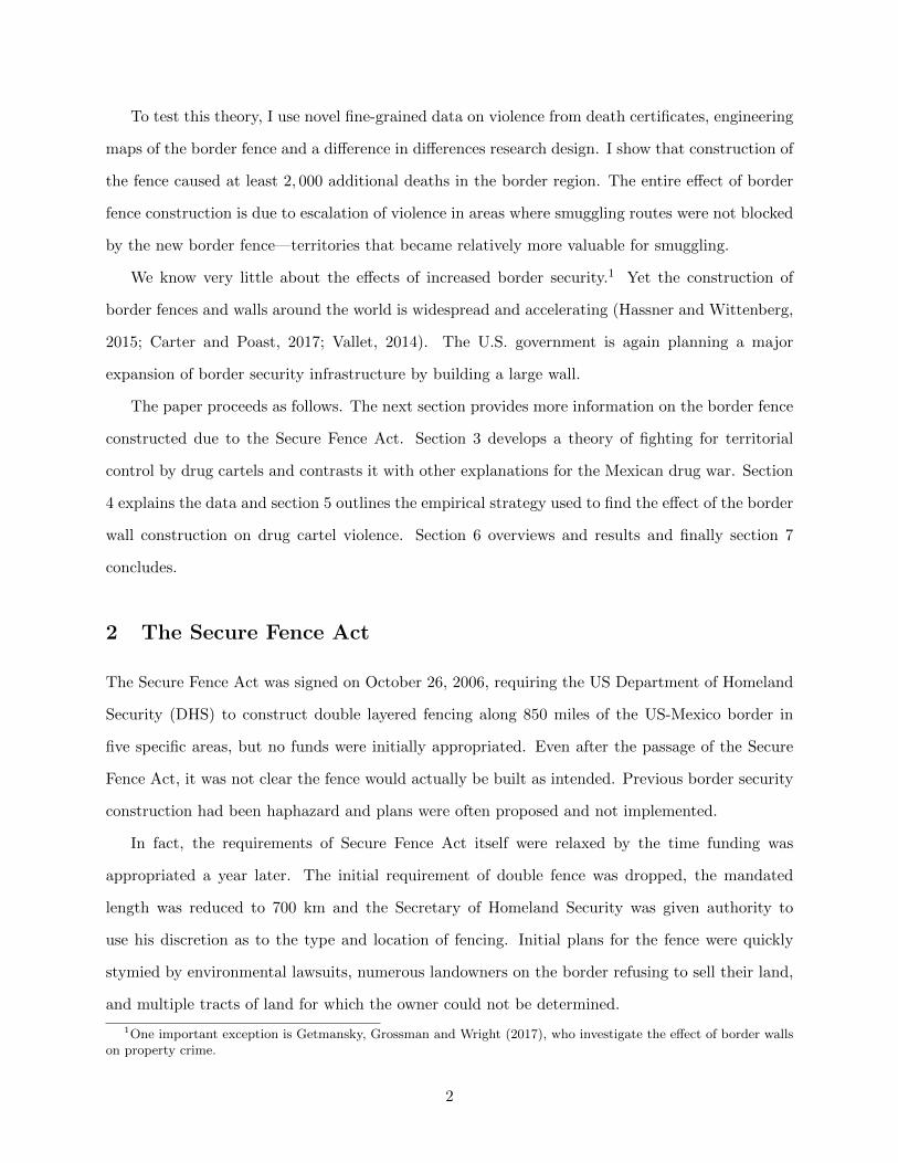
Figure 1: Violence in Mexico over time.

By September 30, 2007 only 2.32 miles of fencing had been constructed. Thus, it would not

have been obvious to leaders of drug cartels that the Secure Fence Act would have a major impact

on them. Only the actual construction of the fence indicated that a border fence of any significant

size would actually be built. The exact location of the fence remained a secret. During construction

plans continued to change due to cost overruns. The plans for the border fence were only released

in 2011—after the fence was complete—after a long Freedom of Information Act lawsuit.

3 Explaining Violence in the Mexican Drug War

The intensity of the Mexican drug war increased dramatically in 2007, especially near the US border.

Numerous explanations for the escalation of the drug war have been offered. These include the

election of PAN mayors (Dell, 2015), the killing or arrest of cartel leaders (Calderon et al., 2015),

uncertainty about government corruption(Zachary and Spaniel, 2015), and events in Colombia

(Castillo, Mejia and Restrepo, 2013). I present another explanation: the construction of the border

fence on the US-Mexico border changed the value of territory to drug cartels.

It is well known that inter-cartel violence is driven by competition between drug cartels over

territory (Beittel, 2015). Territorial control is valuable to cartels as locations to grow and process

3

Month

Hom

icid

es (

% J

an 2

002

leve

l)

Jan 2002 Jan 2005 Jan 2008 Jan 2011 Jan 2014

02

46

810

Border FenceConstruction

≤ 10 km from US≥ 100 km from US

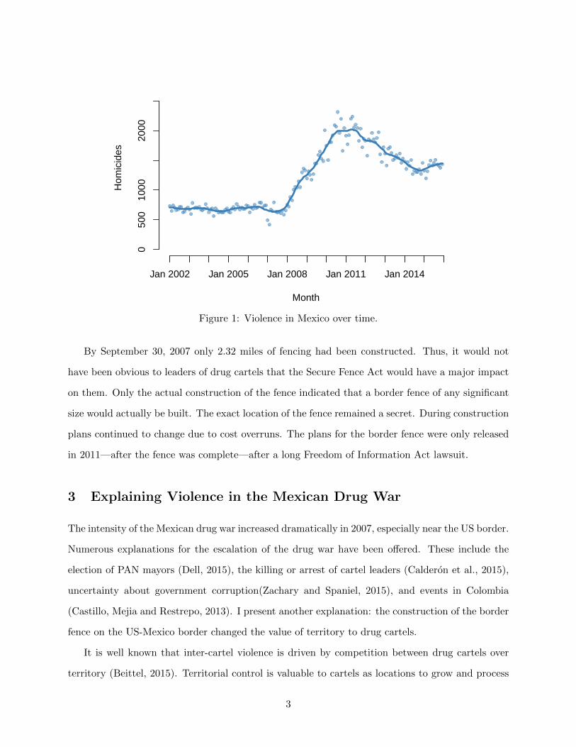
Figure 2: Violence in Mexico near and far from the U.S. border.

drugs, remain safe from the government, and smuggle drugs into and out of Mexico. The border

region is especially valuable for its smuggling routes into the US. Physical border security, including

walls and fences, changes the cost of smuggling by drug cartels. Often cartels make significant

investments into circumventing border security. Multiple tunnels crossing the border between

Tijuana and San Diego have been discovered.

Constructing a border wall changes the relative value of territory near the border for drug

cartels, which upsets the equilibrium of territorial control. Fighting over territory can be limited

by agreements between cartels about territorial control. This is ideal for cartels for the same reason

it is for states: because negotiating agreements over territorial control is less costly than fighting

(Fearon, 1995). This is not unusual. Non-state actors reaching agreements about territorial control

and fighting when those agreements break down has be identified in organized crime (Klein, 1997;

Gambetta, 1996, 7) and insurgent groups (Mampilly, 2011; Staniland, 2012).

Territory near the border is used by drug cartels to smuggle drugs across the border. Border

fences directly affect the costs of smuggling. When a fence blocks a smuggling routes from a

particular area, smuggling from that area becomes more costly and smuggling from other areas

where routes across the border have not been blocked by the new fence become relatively less

4

costly. The change in the cost of smuggling directly affects the value of territory near the border

to drug cartels. Areas near the new fence become less valuable to cartels and other areas with

alternative smuggling routes become relatively more valuable. This shock to the value of territory

controlled by drug cartels may cause cartels to fight over nearly more valuable territory.2 If the

fighting is actually caused by changes in the value of territory caused by the border fence, there

should be increased competition over territory where smuggling routes were not blocked by the

construction of the border fence.

Not only were there changes in the expected future value of territory to drug cartels it was

unknown how they would be affected when the border fence was complete. When construction of

the border fence began, there was some uncertainty about exactly where it would be located. Even

when cartels could guess where the fence was likely to be built, uncertainty about how construction

of the fence would affect smuggling revenues—both their own and the revenues of competing cartels.

This uncertainty about future power and resources can lead to fighting.3 However, fighting reveals

which cartels are stronger, enabling them to reach agreements that were previously impossible

due to differing beliefs about the balance of power (Fearon, 1995; Reiter, 2003; Powell, 2006). I

hypothesize that cartels will fight over territory in the border region only while uncertainty about

the long-term value of territory near the border remains—while the fence is being constructed.

Once the relative value of territory is known and stops changing, new agreements can be reached,

limiting the violence.

This implies both partial equilibrium and general equilibrium hypotheses. The partial equilib-

rium hypothesis is that near the border, violence will be displaced from territories where smuggling

routes are blocked by the newly constructed border fence to areas where the value of the territory

for smuggling has not been reduced by the border fence. The general equilibrium hypothesis is

that the overall effect of the border fence on violence—combining areas where smuggling routes

are blocked by the new border fence and other areas where smuggling could be displaced—will be

positive while the fence is under construction.

2Changes in revenue to non-state actors has been shown to affect the production of violence in numerous othercontexts (Berman et al., 2011; Dube and Vargas, 2013; Wright, 2016).

3In other contexts, it has been shown that expectations about the future matter for territorial control by non-state actors (Sanchez de la Sierra, 2015) and uncertainty has been linked to instability and increased risk of violence(Acharya and Lee, 2016).

5

4 Data on Drug War Violence and Construction of the Border

Fence

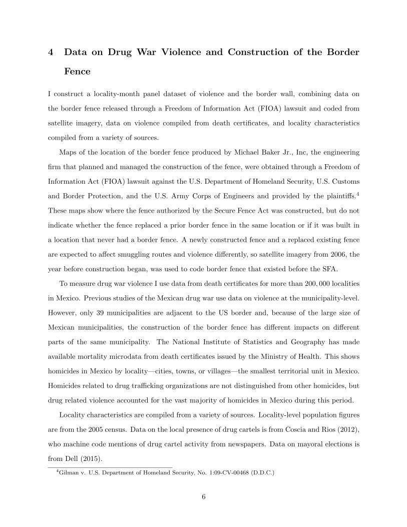
I construct a locality-month panel dataset of violence and the border wall, combining data on

the border fence released through a Freedom of Information Act (FIOA) lawsuit and coded from

satellite imagery, data on violence compiled from death certificates, and locality characteristics

compiled from a variety of sources.

Maps of the location of the border fence produced by Michael Baker Jr., Inc, the engineering

firm that planned and managed the construction of the fence, were obtained through a Freedom of

Information Act (FIOA) lawsuit against the U.S. Department of Homeland Security, U.S. Customs

and Border Protection, and the U.S. Army Corps of Engineers and provided by the plaintiffs.4

These maps show where the fence authorized by the Secure Fence Act was constructed, but do not

indicate whether the fence replaced a prior border fence in the same location or if it was built in

a location that never had a border fence. A newly constructed fence and a replaced existing fence

are expected to affect smuggling routes and violence differently, so satellite imagery from 2006, the

year before construction began, was used to code border fence that existed before the SFA.

To measure drug war violence I use data from death certificates for more than 200, 000 localities

in Mexico. Previous studies of the Mexican drug war use data on violence at the municipality-level.

However, only 39 municipalities are adjacent to the US border and, because of the large size of

Mexican municipalities, the construction of the border fence has different impacts on different

parts of the same municipality. The National Institute of Statistics and Geography has made

available mortality microdata from death certificates issued by the Ministry of Health. This shows

homicides in Mexico by locality—cities, towns, or villages—the smallest territorial unit in Mexico.

Homicides related to drug trafficking organizations are not distinguished from other homicides, but

drug related violence accounted for the vast majority of homicides in Mexico during this period.

Locality characteristics are compiled from a variety of sources. Locality-level population figures

are from the 2005 census. Data on the local presence of drug cartels is from Coscia and Rios (2012),

who machine code mentions of drug cartel activity from newspapers. Data on mayoral elections is

from Dell (2015).

4Gilman v. U.S. Department of Homeland Security, No. 1:09-CV-00468 (D.D.C.)

6

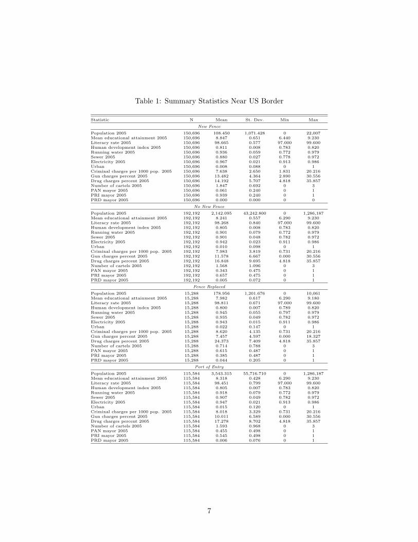
Table 1: Summary Statistics Near US Border

Statistic N Mean St. Dev. Min Max

New Fence

Population 2005 150,696 108.450 1,071.428 0 22,007Mean educational attainment 2005 150,696 8.847 0.651 6.440 9.230Literacy rate 2005 150,696 98.665 0.577 97.000 99.600Human development index 2005 150,696 0.811 0.008 0.783 0.820Running water 2005 150,696 0.936 0.059 0.772 0.979Sewer 2005 150,696 0.880 0.027 0.778 0.972Electricity 2005 150,696 0.967 0.021 0.913 0.986Urban 150,696 0.008 0.088 0 1Criminal charges per 1000 pop. 2005 150,696 7.638 2.650 1.831 20.216Gun charges percent 2005 150,696 13.482 4.364 2.890 30.556Drug charges percent 2005 150,696 14.192 5.707 4.818 35.857Number of cartels 2005 150,696 1.847 0.692 0 3PAN mayor 2005 150,696 0.061 0.240 0 1PRI mayor 2005 150,696 0.939 0.240 0 1PRD mayor 2005 150,696 0.000 0.000 0 0

No New Fence

Population 2005 192,192 2,142.095 43,242.800 0 1,286,187Mean educational attainment 2005 192,192 8.241 0.557 6.290 9.230Literacy rate 2005 192,192 98.268 0.840 97.000 99.600Human development index 2005 192,192 0.805 0.008 0.783 0.820Running water 2005 192,192 0.901 0.079 0.772 0.979Sewer 2005 192,192 0.901 0.048 0.782 0.972Electricity 2005 192,192 0.942 0.023 0.911 0.986Urban 192,192 0.010 0.098 0 1Criminal charges per 1000 pop. 2005 192,192 7.983 3.819 0.731 20.216Gun charges percent 2005 192,192 11.578 6.667 0.000 30.556Drug charges percent 2005 192,192 16.848 9.695 4.818 35.857Number of cartels 2005 192,192 1.568 1.096 0 3PAN mayor 2005 192,192 0.343 0.475 0 1PRI mayor 2005 192,192 0.657 0.475 0 1PRD mayor 2005 192,192 0.005 0.072 0 1

Fence Replaced

Population 2005 15,288 178.956 1,201.676 0 10,061Mean educational attainment 2005 15,288 7.982 0.617 6.290 9.180Literacy rate 2005 15,288 98.811 0.671 97.000 99.600Human development index 2005 15,288 0.800 0.007 0.789 0.820Running water 2005 15,288 0.945 0.055 0.797 0.979Sewer 2005 15,288 0.935 0.049 0.782 0.972Electricity 2005 15,288 0.943 0.015 0.911 0.986Urban 15,288 0.022 0.147 0 1Criminal charges per 1000 pop. 2005 15,288 8.620 4.135 0.731 20.216Gun charges percent 2005 15,288 7.457 4.597 0.000 18.327Drug charges percent 2005 15,288 24.373 7.409 4.818 35.857Number of cartels 2005 15,288 0.714 0.788 0 3PAN mayor 2005 15,288 0.615 0.487 0 1PRI mayor 2005 15,288 0.385 0.487 0 1PRD mayor 2005 15,288 0.044 0.205 0 1

Port of Entry

Population 2005 115,584 3,543.315 55,716.710 0 1,286,187Mean educational attainment 2005 115,584 8.318 0.428 6.290 9.230Literacy rate 2005 115,584 98.451 0.799 97.000 99.600Human development index 2005 115,584 0.805 0.007 0.783 0.820Running water 2005 115,584 0.918 0.079 0.772 0.979Sewer 2005 115,584 0.907 0.049 0.782 0.972Electricity 2005 115,584 0.947 0.021 0.913 0.986Urban 115,584 0.015 0.120 0 1Criminal charges per 1000 pop. 2005 115,584 8.018 3.329 0.731 20.216Gun charges percent 2005 115,584 10.011 6.589 0.000 30.556Drug charges percent 2005 115,584 17.278 8.702 4.818 35.857Number of cartels 2005 115,584 1.593 0.968 0 3PAN mayor 2005 115,584 0.455 0.498 0 1PRI mayor 2005 115,584 0.545 0.498 0 1PRD mayor 2005 115,584 0.006 0.076 0 1

7

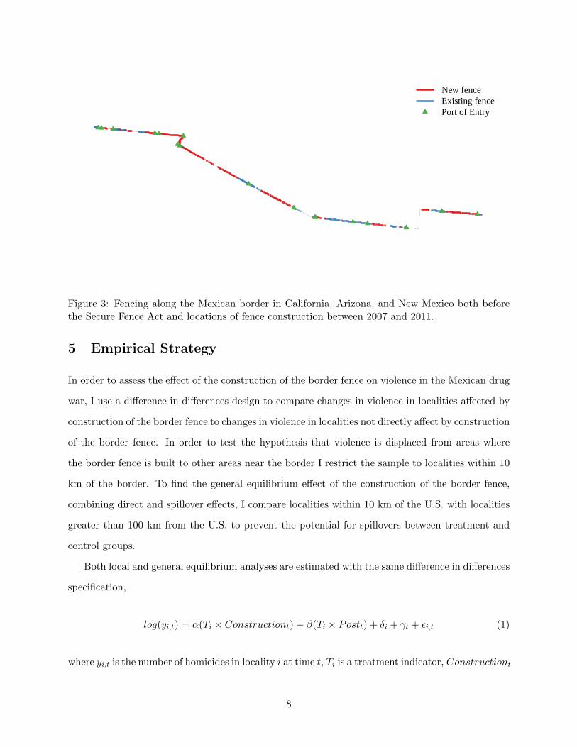
New fenceExisting fencePort of Entry

Figure 3: Fencing along the Mexican border in California, Arizona, and New Mexico both beforethe Secure Fence Act and locations of fence construction between 2007 and 2011.

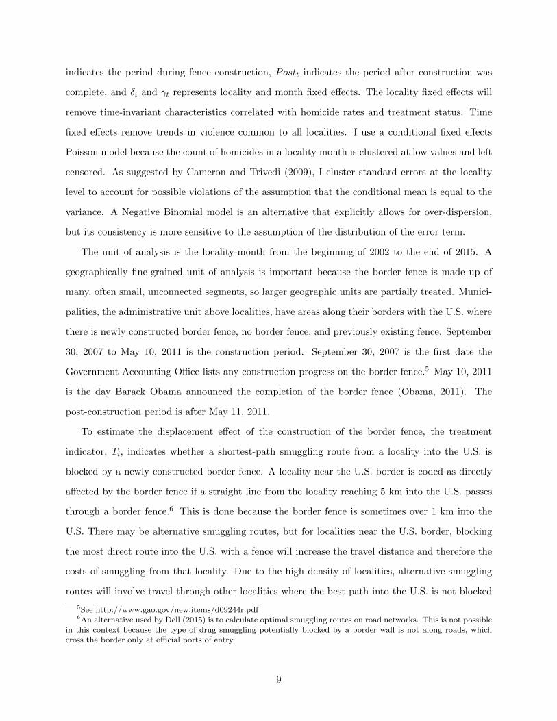
5 Empirical Strategy

In order to assess the effect of the construction of the border fence on violence in the Mexican drug

war, I use a difference in differences design to compare changes in violence in localities affected by

construction of the border fence to changes in violence in localities not directly affect by construction

of the border fence. In order to test the hypothesis that violence is displaced from areas where

the border fence is built to other areas near the border I restrict the sample to localities within 10

km of the border. To find the general equilibrium effect of the construction of the border fence,

combining direct and spillover effects, I compare localities within 10 km of the U.S. with localities

greater than 100 km from the U.S. to prevent the potential for spillovers between treatment and

control groups.

Both local and general equilibrium analyses are estimated with the same difference in differences

specification,

log(yi,t) = α(Ti × Constructiont) + β(Ti × Postt) + δi + γt + εi,t (1)

where yi,t is the number of homicides in locality i at time t, Ti is a treatment indicator, Constructiont

8

indicates the period during fence construction, Postt indicates the period after construction was

complete, and δi and γt represents locality and month fixed effects. The locality fixed effects will

remove time-invariant characteristics correlated with homicide rates and treatment status. Time

fixed effects remove trends in violence common to all localities. I use a conditional fixed effects

Poisson model because the count of homicides in a locality month is clustered at low values and left

censored. As suggested by Cameron and Trivedi (2009), I cluster standard errors at the locality

level to account for possible violations of the assumption that the conditional mean is equal to the

variance. A Negative Binomial model is an alternative that explicitly allows for over-dispersion,

but its consistency is more sensitive to the assumption of the distribution of the error term.

The unit of analysis is the locality-month from the beginning of 2002 to the end of 2015. A

geographically fine-grained unit of analysis is important because the border fence is made up of

many, often small, unconnected segments, so larger geographic units are partially treated. Munici-

palities, the administrative unit above localities, have areas along their borders with the U.S. where

there is newly constructed border fence, no border fence, and previously existing fence. September

30, 2007 to May 10, 2011 is the construction period. September 30, 2007 is the first date the

Government Accounting Office lists any construction progress on the border fence.5 May 10, 2011

is the day Barack Obama announced the completion of the border fence (Obama, 2011). The

post-construction period is after May 11, 2011.

To estimate the displacement effect of the construction of the border fence, the treatment

indicator, Ti, indicates whether a shortest-path smuggling route from a locality into the U.S. is

blocked by a newly constructed border fence. A locality near the U.S. border is coded as directly

affected by the border fence if a straight line from the locality reaching 5 km into the U.S. passes

through a border fence.6 This is done because the border fence is sometimes over 1 km into the

U.S. There may be alternative smuggling routes, but for localities near the U.S. border, blocking

the most direct route into the U.S. with a fence will increase the travel distance and therefore the

costs of smuggling from that locality. Due to the high density of localities, alternative smuggling

routes will involve travel through other localities where the best path into the U.S. is not blocked

5See http://www.gao.gov/new.items/d09244r.pdf6An alternative used by Dell (2015) is to calculate optimal smuggling routes on road networks. This is not possible

in this context because the type of drug smuggling potentially blocked by a border wall is not along roads, whichcross the border only at official ports of entry.

9

by a border fence.

The set of localities potentially affected by construction of the border fence is conservatively

restricted to localities within 10 km of the border with California, Arizona, and New Mexico.

Localities very close to the U.S. border are likely to be the most valuable for smuggling, as smugglers

must cross these areas to reach the U.S. It is less clear how small changes in the border fence might

affect smuggling from localities farther from the U.S. Localities near the Texas border are not

considered for three reasons. First, less than 15 km of the SFA fence was constructed along the Texas

border because the Rio Grande provides a natural barrier. These localities are a poor control group

because DHS’s strategic decision not to build a border fence in these areas indicates differences that

might affect trends. With the exception of Juarez, areas of Mexico bordering Texas are much more

rural and poorer than areas in Mexico bordering California, Arizona, and New Mexico. Second, the

border fence that was built in Texas was delayed by cost overruns and lawsuits. All of the border

fence built in California, Arizona, and New Mexico was built between September 30, 2007 and

May 10, 2011, but fence construction in some parts of Texas did not start until 2013. It is unclear

from the data DHS has released exactly when different border fences in Texas were built, which is

necessary to code the construction and post-construction period indicators. Third, because of the

huge distance, the Texas border would be an unlikely location to displace smuggling routes from

localities near California, Arizona, and New Mexico. Nearer areas where no new border fence was

built are likely to be better alternative smuggling routes.

To estimate the general equilibrium effect of the construction of the border fence it is necessary

to compare the change in violence both in areas directly affected by the border fence and and

areas where smuggling might have be displaced and which become more valuable to drug cartels

to violence in areas unaffected by construction of the border fence. This means the treatment

group should be all localities near the U.S. border, control of which is either relatively more or less

valuable to drug cartels after construction of the border fence. Therefore, the treatment indicator

for the general equilibrium analysis, Ti, indicates whether a locality is within 10 km of the border

with California, Arizona, or New Mexico. Texas is again excluded, for the reasons given above and

for consistency.

10

6 Results

The theory presented in section 3 implies that the shock to the value of territory controlled by drug

cartels due to the construction of the border fence will cause competition between drug cartels

for territorial control. This leads to the hypotheses that construction of the border fence will (1)

displace violence from localities where border fence construction increases the costs of smuggling

and thus lowers the value of territorial control to areas where the relative value of territorial control

has increased and (2) increase the overall level of violence in the border region. These effects are

expected during the period when the border fence is under construction because the construction

plans—and therefore the final value of territorial control—were unknown. Once construction was

complete the relative value of different territories became know to the drug cartels and agreements

over territorial control between cartels could reduce fighting, so violence is expected to be lower

after construction is complete compared to the period when the border fence was being constructed.

6.1 Displacement Effects of Border Fence Construction

In this section I examine the hypothesis that construction of the border fence displaced violence

from areas where the new fence increased the difficulty of smuggling and lowered the value of the

territory to drug cartels to other areas near the border where border security was not increased.

Areas not next to newly constructed border fence are alternative smuggling routes, so the relative

value of these territories to drug smugglers will increase. Violence is expected to increase these

alternatives due to competition between drug cartels for control of these territories.

All localities near the border where a new fence is not constructed are alternatives to localities

where smuggling is more costly due to border fence construction. These include areas where no

fence is constructed, areas where a prior border fence existed, and ports of entry into the U.S. The

cost of using these smuggling routes has not changed, but alternatives are more costly after the

SFA fence is built, so these areas become relatively more valuable to drug cartels.

Table 2 shows difference in differences estimates of equation 1 for localities within 10 km of the

U.S. Column (1) shows that Mexican localities next to a newly constructed fence along the U.S.

border experienced an additional 1.282 log-point, or 72.3 percent, decrease in violence compared

to localities where no new fence was built during the period of fence construction and a 0.727

11

log-point, or 51.6 percent, reduction in violence in the period after construction of the fence was

completed.

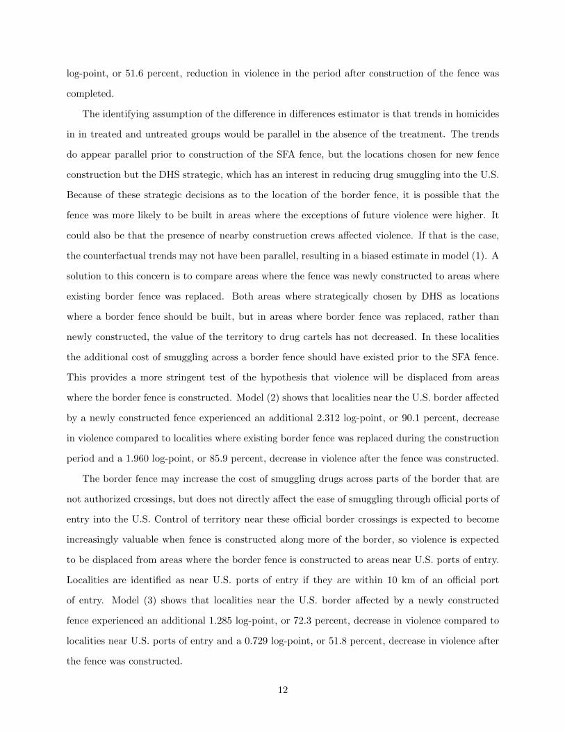
The identifying assumption of the difference in differences estimator is that trends in homicides

in in treated and untreated groups would be parallel in the absence of the treatment. The trends

do appear parallel prior to construction of the SFA fence, but the locations chosen for new fence

construction but the DHS strategic, which has an interest in reducing drug smuggling into the U.S.

Because of these strategic decisions as to the location of the border fence, it is possible that the

fence was more likely to be built in areas where the exceptions of future violence were higher. It

could also be that the presence of nearby construction crews affected violence. If that is the case,

the counterfactual trends may not have been parallel, resulting in a biased estimate in model (1). A

solution to this concern is to compare areas where the fence was newly constructed to areas where

existing border fence was replaced. Both areas where strategically chosen by DHS as locations

where a border fence should be built, but in areas where border fence was replaced, rather than

newly constructed, the value of the territory to drug cartels has not decreased. In these localities

the additional cost of smuggling across a border fence should have existed prior to the SFA fence.

This provides a more stringent test of the hypothesis that violence will be displaced from areas

where the border fence is constructed. Model (2) shows that localities near the U.S. border affected

by a newly constructed fence experienced an additional 2.312 log-point, or 90.1 percent, decrease

in violence compared to localities where existing border fence was replaced during the construction

period and a 1.960 log-point, or 85.9 percent, decrease in violence after the fence was constructed.

The border fence may increase the cost of smuggling drugs across parts of the border that are

not authorized crossings, but does not directly affect the ease of smuggling through official ports of

entry into the U.S. Control of territory near these official border crossings is expected to become

increasingly valuable when fence is constructed along more of the border, so violence is expected

to be displaced from areas where the border fence is constructed to areas near U.S. ports of entry.

Localities are identified as near U.S. ports of entry if they are within 10 km of an official port

of entry. Model (3) shows that localities near the U.S. border affected by a newly constructed

fence experienced an additional 1.285 log-point, or 72.3 percent, decrease in violence compared to

localities near U.S. ports of entry and a 0.729 log-point, or 51.8 percent, decrease in violence after

the fence was constructed.

12

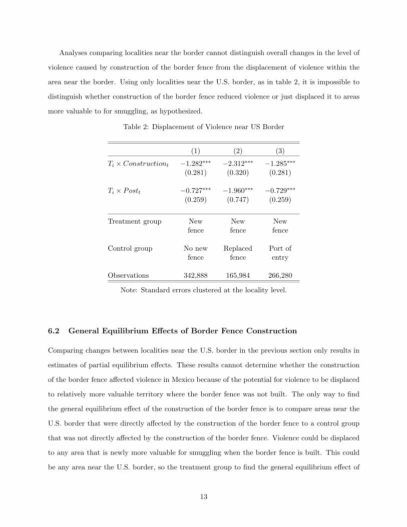
Analyses comparing localities near the border cannot distinguish overall changes in the level of

violence caused by construction of the border fence from the displacement of violence within the

area near the border. Using only localities near the U.S. border, as in table 2, it is impossible to

distinguish whether construction of the border fence reduced violence or just displaced it to areas

more valuable to for smuggling, as hypothesized.

Table 2: Displacement of Violence near US Border

(1) (2) (3)

Ti × Constructiont −1.282∗∗∗ −2.312∗∗∗ −1.285∗∗∗

(0.281) (0.320) (0.281)

Ti × Postt −0.727∗∗∗ −1.960∗∗∗ −0.729∗∗∗

(0.259) (0.747) (0.259)

Treatment group New New Newfence fence fence

Control group No new Replaced Port offence fence entry

Observations 342,888 165,984 266,280

Note: Standard errors clustered at the locality level.

6.2 General Equilibrium Effects of Border Fence Construction

Comparing changes between localities near the U.S. border in the previous section only results in

estimates of partial equilibrium effects. These results cannot determine whether the construction

of the border fence affected violence in Mexico because of the potential for violence to be displaced

to relatively more valuable territory where the border fence was not built. The only way to find

the general equilibrium effect of the construction of the border fence is to compare areas near the

U.S. border that were directly affected by the construction of the border fence to a control group

that was not directly affected by the construction of the border fence. Violence could be displaced

to any area that is newly more valuable for smuggling when the border fence is built. This could

be any area near the U.S. border, so the treatment group to find the general equilibrium effect of

13

Month

Mea

n ho

mic

ides

(%

pre

−tr

eatm

ent l

evel

)

Jan 2002 Jan 2005 Jan 2008 Jan 2011 Jan 2014

02

46

810

Border FenceConstruction

New fenceNot new fence

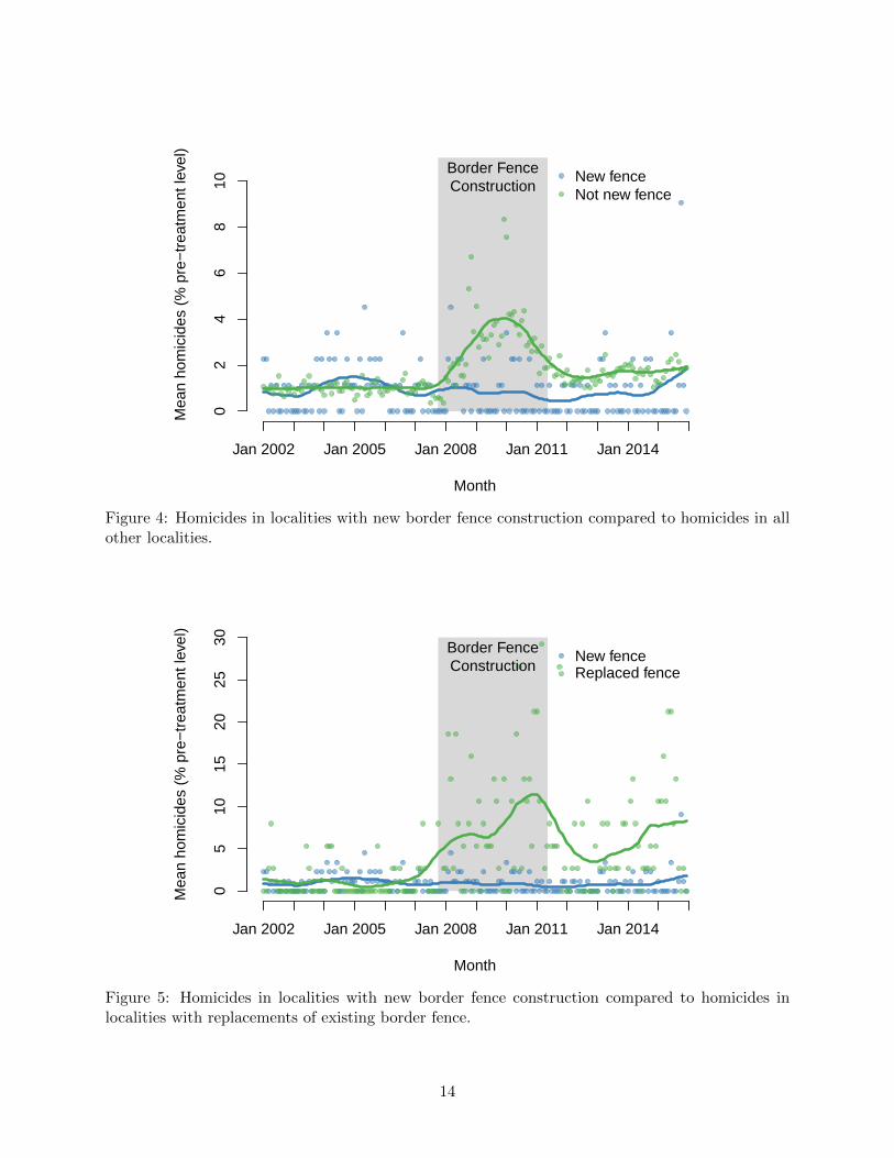
Figure 4: Homicides in localities with new border fence construction compared to homicides in allother localities.

Month

Mea

n ho

mic

ides

(%

pre

−tr

eatm

ent l

evel

)

Jan 2002 Jan 2005 Jan 2008 Jan 2011 Jan 2014

05

1015

2025

30 Border FenceConstruction

New fenceReplaced fence

Figure 5: Homicides in localities with new border fence construction compared to homicides inlocalities with replacements of existing border fence.

14

Month

Mea

n ho

mic

ides

(%

pre

−tr

eatm

ent l

evel

)

Jan 2002 Jan 2005 Jan 2008 Jan 2011 Jan 2014

02

46

810

Border FenceConstruction

New fenceUS port of entry

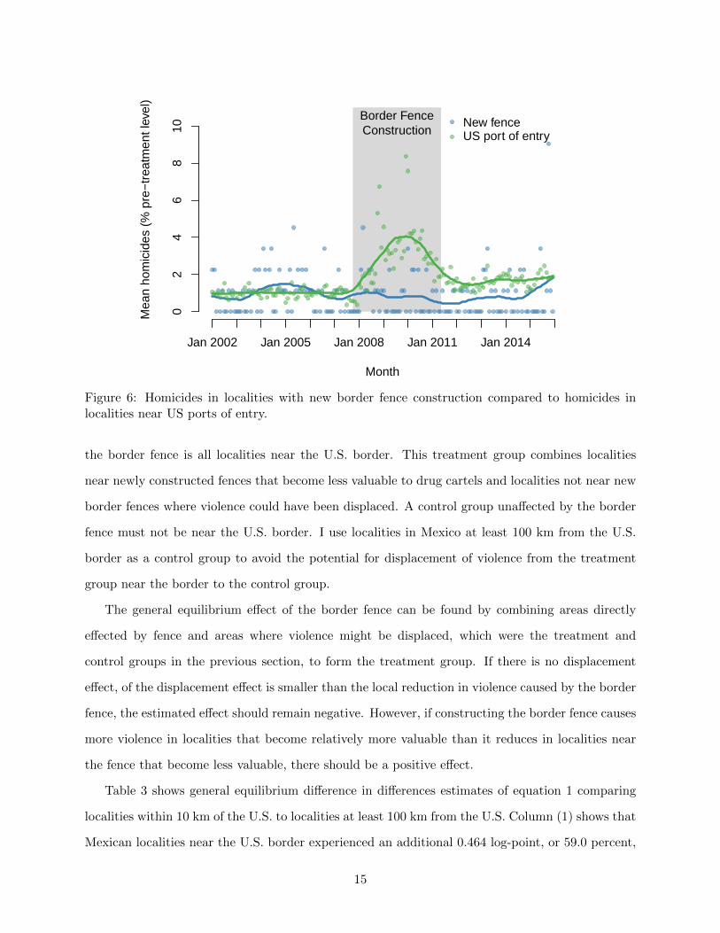
Figure 6: Homicides in localities with new border fence construction compared to homicides inlocalities near US ports of entry.

the border fence is all localities near the U.S. border. This treatment group combines localities

near newly constructed fences that become less valuable to drug cartels and localities not near new

border fences where violence could have been displaced. A control group unaffected by the border

fence must not be near the U.S. border. I use localities in Mexico at least 100 km from the U.S.

border as a control group to avoid the potential for displacement of violence from the treatment

group near the border to the control group.

The general equilibrium effect of the border fence can be found by combining areas directly

effected by fence and areas where violence might be displaced, which were the treatment and

control groups in the previous section, to form the treatment group. If there is no displacement

effect, of the displacement effect is smaller than the local reduction in violence caused by the border

fence, the estimated effect should remain negative. However, if constructing the border fence causes

more violence in localities that become relatively more valuable than it reduces in localities near

the fence that become less valuable, there should be a positive effect.

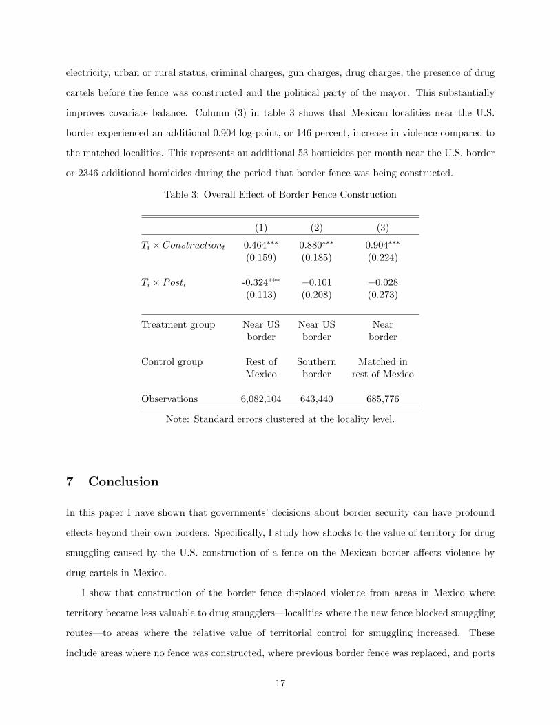
Table 3 shows general equilibrium difference in differences estimates of equation 1 comparing

localities within 10 km of the U.S. to localities at least 100 km from the U.S. Column (1) shows that

Mexican localities near the U.S. border experienced an additional 0.464 log-point, or 59.0 percent,

15

increase in violence compared to a 1 percent sample of localities not near the U.S. border during

the period of fence construction and a 0.324 log-point, or 27.7 percent, reduction in violence in

the period after construction of the fence was completed. An average of 36.3 homicides per month

occurred within 10 km of the U.S. states of California, Arizona, and New Mexico, so an additional

59 percent increase represents an additional 942 homicides during the period that border fence was

being constructed.

Difference in differences estimates relies on the assumption that if the border fence had not

been built, violence in the border region and violence in the control region would have had the

same trends over time. The main concern in selecting a control group is that border localities and

control localities may differ in ways related to the trends in violence over time. There is a concern

that all localities in Mexico far from the border is not an ideal control group for localities near the

border that may have been affected, directly or through displacement, by the construction of the

border fence. Pre-treatment trends appear parallel, but it may be the that areas near the border

are unique because of the value of the territory for cross-border smuggling and that this affects

trends. This suggests localities near Mexico’s southern border with Guatemala and Belize as a

control group. Drugs are smuggled across this border by cartels, but no border fence was build

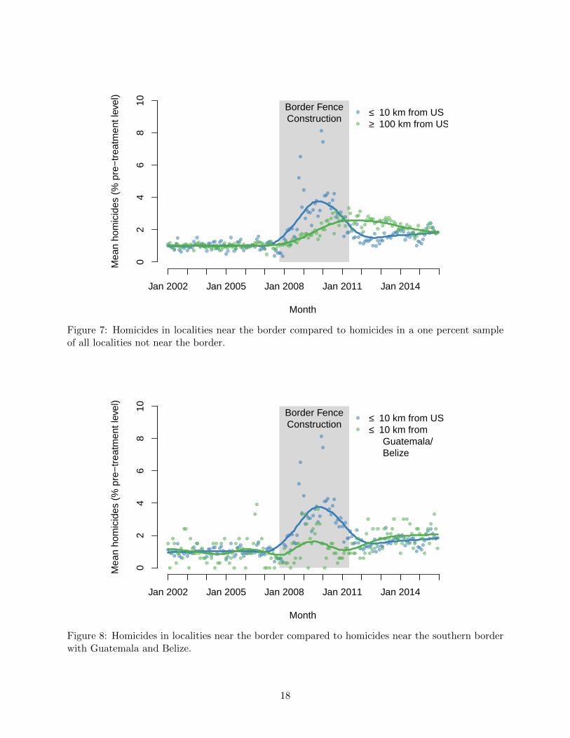
along Mexico’s southern border. Column (2) in table 3 shows that Mexican localities near the U.S.

border experienced an additional 0.880 log-point, or 141.1 percent, increase in violence compared

to localities near Mexico’s southern border. This represents an additional 51 homicides per month

near the U.S. border or 2252 additional homicides during the period that border fence was being

constructed.

It may be that localities near the U.S. border differ in ways that affect trends in homicides from

localities that are not near the border. Localities near the U.S. border differed prior to construction

of the border fence from those far from the border in ways previous research has indicated may

affect drug war violence. Localities near the border are on average richer, better educated, and

differ in crime rates, drug cartel presence, and political parties elected. To alleviate the concern that

the results may be driven by these differences, I construct control group from localities at least 100

km from the U.S border matched on pre-treatment covariates. I use nearest neighbor propensity

score matching without replacement to match on pre-treatment population, average education

level, literacy rate, the human development index, indices of access to running water, sewer, and

16

electricity, urban or rural status, criminal charges, gun charges, drug charges, the presence of drug

cartels before the fence was constructed and the political party of the mayor. This substantially

improves covariate balance. Column (3) in table 3 shows that Mexican localities near the U.S.

border experienced an additional 0.904 log-point, or 146 percent, increase in violence compared to

the matched localities. This represents an additional 53 homicides per month near the U.S. border

or 2346 additional homicides during the period that border fence was being constructed.

Table 3: Overall Effect of Border Fence Construction

(1) (2) (3)

Ti × Constructiont 0.464∗∗∗ 0.880∗∗∗ 0.904∗∗∗

(0.159) (0.185) (0.224)

Ti × Postt -0.324∗∗∗ −0.101 −0.028(0.113) (0.208) (0.273)

Treatment group Near US Near US Nearborder border border

Control group Rest of Southern Matched inMexico border rest of Mexico

Observations 6,082,104 643,440 685,776

Note: Standard errors clustered at the locality level.

7 Conclusion

In this paper I have shown that governments’ decisions about border security can have profound

effects beyond their own borders. Specifically, I study how shocks to the value of territory for drug

smuggling caused by the U.S. construction of a fence on the Mexican border affects violence by

drug cartels in Mexico.

I show that construction of the border fence displaced violence from areas in Mexico where

territory became less valuable to drug smugglers—localities where the new fence blocked smuggling

routes—to areas where the relative value of territorial control for smuggling increased. These

include areas where no fence was constructed, where previous border fence was replaced, and ports

17

Month

Mea

n ho

mic

ides

(%

pre

−tr

eatm

ent l

evel

)

Jan 2002 Jan 2005 Jan 2008 Jan 2011 Jan 2014

02

46

810 Border Fence

Construction≤ 10 km from US≥ 100 km from US

Figure 7: Homicides in localities near the border compared to homicides in a one percent sampleof all localities not near the border.

Month

Mea

n ho

mic

ides

(%

pre

−tr

eatm

ent l

evel

)

Jan 2002 Jan 2005 Jan 2008 Jan 2011 Jan 2014

02

46

810 Border Fence

Construction≤ 10 km from US≤ 10 km from Guatemala/ Belize

Figure 8: Homicides in localities near the border compared to homicides near the southern borderwith Guatemala and Belize.

18

Month

Mea

n ho

mic

ides

(%

pre

−tr

eatm

ent l

evel

)

Jan 2002 Jan 2005 Jan 2008 Jan 2011 Jan 2014

02

46

810 Border Fence

Construction≤ 10 km from US≥ 100 km from US

Figure 9: Homicides in localities near the border compared to homicides in a propensity scorematched set of localities not near the border.

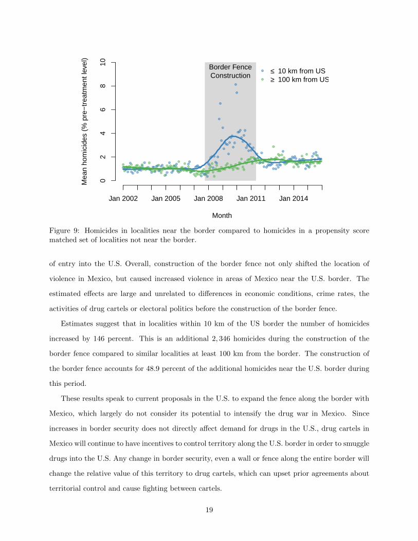
of entry into the U.S. Overall, construction of the border fence not only shifted the location of

violence in Mexico, but caused increased violence in areas of Mexico near the U.S. border. The

estimated effects are large and unrelated to differences in economic conditions, crime rates, the

activities of drug cartels or electoral politics before the construction of the border fence.

Estimates suggest that in localities within 10 km of the US border the number of homicides

increased by 146 percent. This is an additional 2, 346 homicides during the construction of the

border fence compared to similar localities at least 100 km from the border. The construction of

the border fence accounts for 48.9 percent of the additional homicides near the U.S. border during

this period.

These results speak to current proposals in the U.S. to expand the fence along the border with

Mexico, which largely do not consider its potential to intensify the drug war in Mexico. Since

increases in border security does not directly affect demand for drugs in the U.S., drug cartels in

Mexico will continue to have incentives to control territory along the U.S. border in order to smuggle

drugs into the U.S. Any change in border security, even a wall or fence along the entire border will

change the relative value of this territory to drug cartels, which can upset prior agreements about

territorial control and cause fighting between cartels.

19

By demonstrating that construction of the border fence caused drug cartel violence, I provide

evidence that non-state actors fight to control territory and that the value of the territory af-

fects their willingness to fight. The increase in violence persisted only while the fence was under

construction—while exact location and effects on smuggling revenues remained uncertain. This

suggests that uncertainty over the future value of territory for smuggling prevented drug cartels

from reaching agreements about territorial control that would have prevented fighting between

cartels.

References

Acemoglu, Daron and James A Robinson. 2005. Economic origins of dictatorship and democracy.

Cambridge University Press.

Acharya, Avidit and Alexander Lee. 2016. “Path Dependence in European Development: Medieval

Politics, Conflict, and State-Building.”.

Bazzi, Samuel and Christopher Blattman. 2014. “Economic shocks and conflict: Evidence from

commodity prices.” American Economic Journal: Macroeconomics 6(4):1–38.

Beittel, June. 2015. “Mexico: Organized crime and drug trafficking organizations.” Washington

DC: Congressional Research Service .

Berman, Eli, Michael Callen, Joseph H Felter and Jacob N Shapiro. 2011. “Do working men rebel?

Insurgency and unemployment in Afghanistan, Iraq, and the Philippines.” Journal of Conflict

Resolution 55(4):496–528.

Besley, Timothy J and Torsten Persson. 2008. “The incidence of civil war: Theory and evidence.”.

Borkowski, Mark, Michael Fisher and Michael Kostelnik. 2011. “After SBInet - the Future of

Technology on the Border.” Testimony before the United States House Committee on Homeland

Security, Subcommittee on Border and Maritime Security . March 15.

URL: https://www.dhs.gov/news/2011/03/15/written-testimony-cbp-house-homeland-security-

subcommittee-border-and-maritime

20

Bruckner, Markus and Antonio Ciccone. 2010. “International commodity prices, growth and the

outbreak of civil war in Sub-Saharan Africa.” The Economic Journal 120(544):519–534.

Bush, George W. 2006. “Bush’s Speech on Immigration.” The New York Times . March 15.

URL: http://www.nytimes.com/2006/05/15/washington/15text-bush.html

Calderon, Gabriela, Gustavo Robles, Alberto Dıaz-Cayeros and Beatriz Magaloni. 2015. “The

beheading of criminal organizations and the dynamics of violence in Mexico.” Journal of Conflict

Resolution 59(8):1455–1485.

Cameron, A Colin and Pravin K Trivedi. 2009. “Microeconometrics with STATA.” College Station,

TX: StataCorp LP .

Carter, David B and Paul Poast. 2017. “Why do states build walls? Political economy, security,

and border stability.” Journal of conflict resolution 61(2):239–270.

Caselli, Francesco, Massimo Morelli and Dominic Rohner. 2015. “The geography of interstate

resource wars.” The Quarterly Journal of Economics 130(1):267–315.

Castillo, Juan Camilo, Daniel Mejia and Pascual Restrepo. 2013. “Illegal drug markets and violence

in Mexico: The causes beyond Calderon.” Universidad de los Andes typescript .

Collier, Paul and Anke Hoeffler. 1998. “On economic causes of civil war.” Oxford economic papers

50(4):563–573.

Coscia, Michele and Viridiana Rios. 2012. Knowing where and how criminal organizations operate

using web content. In Proceedings of the 21st ACM international conference on Information and

knowledge management. ACM pp. 1412–1421.

de la Sierra, Raul Sanchez. 2014. “On the origin of states: Stationary bandits and taxation in

Eastern Congo.”.

Dell, Melissa. 2015. “Trafficking networks and the Mexican drug war.” The American Economic

Review 105(6):1738–1779.

Dube, Oeindrila and Juan F Vargas. 2013. “Commodity price shocks and civil conflict: Evidence

from Colombia.” The Review of Economic Studies 80(4):1384–1421.

21

Fearon, James D. 1995. “Rationalist explanations for war.” International organization 49(3):379–

414.

Fearon, James D. 2005. “Primary commodity exports and civil war.” Journal of conflict Resolution

49(4):483–507.

Gambetta, Diego. 1996. The Sicilian Mafia: the business of private protection. Harvard University

Press.

Getmansky, Anna, Guy Grossman and Austin L. Wright. 2017. “Border Walls and the Economics

of Crime.”.

Hassner, Ron E and Jason Wittenberg. 2015. “Barriers to Entry: Who Builds Fortified Boundaries

and Why?” International Security .

Klein, Malcolm W. 1997. The American street gang: Its nature, prevalence, and control. Oxford

University Press.

Konrad, Kai A and Stergios Skaperdas. 2012. “The Market for Protection and the Origin of the

State.” Economic Theory 50(2):417–443.

Mampilly, Zachariah Cherian. 2011. Rebel rulers: Insurgent governance and civilian life during

war. Cornell University Press.

Miguel, Edward, Shanker Satyanath and Ernest Sergenti. 2004. “Economic shocks and civil conflict:

An instrumental variables approach.” Journal of political Economy 112(4):725–753.

Nielsen, Richard A, Michael G Findley, Zachary S Davis, Tara Candland and Daniel L Nielson.

2011. “Foreign aid shocks as a cause of violent armed conflict.” American Journal of Political

Science 55(2):219–232.

Obama, Barack. 2011. “Remarks by the President on Comprehensive Immigration Reform in El

Paso, Texas.”.

Olson, Mancur. 1993. “Dictatorship, democracy, and development.” American political science

review 87(3):567–576.

22

Powell, Robert. 2006. “War as a commitment problem.” International organization 60(1):169–203.

Reiter, Dan. 2003. “Exploring the bargaining model of war.” Perspectives on Politics 1(1):27–43.

Sanchez de la Sierra, Raul. 2015. “Dis-organizing Violence: On the Ends of the State, Stationary

Bandits and the Time Horizon.” Unpublished manuscript. University of California, Haas School

of Business, Berkeley .

Staniland, Paul. 2012. “States, insurgents, and wartime political orders.” Perspectives on Politics

10(2):243–264.

Vallet, Elisabeth, ed. 2014. Borders, fences and walls: State of insecurity? Ashgate Publishing,

Ltd.

Wright, Austin L. 2016. “Economic Shocks and Rebel Tactics.”.

Zachary, Paul and William Spaniel. 2015. “Getting a Hand By Cutting Them Off: How Uncertainty

over Political Corruption Affects Violence.”.

23