Border following : new definition gives improved borders

T.D. Haig, BE Y. Attikiouzel, BSc, PhD M.D. Alder, MEngSc, PhD

Indexing terms: Algorithm, Image processing, Picture processing and pattern recognition

Abstract: Border following is widely used in the preprocessing of many binary images. Images may be taken to consist of a set of black objects on a white background, or vice versa, and the objects may have holes in them; some of the holes may contain objects, and this may be repeated. Finding the borders of the objects allows considerable compression and has other advantages, but is more difficult than may appear at first sight. In particular, it is not dificult to obtain algorithms which produce reentrant curves as candidate borders, and others which produce borders which are unsatisfactory for various reasons. The paper describes a co-recursive algorithm obtained from a new definition of borders. Because of some counter-intuitive aspects of the subject, it was necessary to prove that the algorithm produces a border in the sense of the paper. Experiments on a variety of images are described, and the results show that the borders described in the paper are generally smaller and better connected than some others.

1 Introduction

Border-following techniques have a wide variety of appli- cations, including picture recognition, topological analysis, object counting and image compression. The present work arose from the reconstruction of biomedical objects from images of sections; such images pose a severe test for border-following algorithms, partly because of the complex shape of the boundaries, and partly because noise often remains after the common noise-reduction techniques have been applied.

We may define a border-following algorithm by suppos- ing that a binary two-dimensional raster image is pre- sented to the algorithm, and some indeterminate number of chain code sequences, of indeterminate length, is output, together with some pixel on each chain code sequence. Not all algorithms are in precisely this form, but enough are equivalent to it, or are variants of it, to justify this as an introductory definition. Such algorithms have been studied by Rosenfeld and Kak [l] and Pavlidis [2 ] , who offer a variety of solutions. More recently, Suzuki and Abe [3] and Ly and Attikiouzel [4] have

Paper 84691 (E4), received 16th July 1991 Mr. Haig and Prof. Attikiouzel are with the Department of Electrical and Electronic Engineering, and Dr. Alder is with the Department of Mathematics, The University of Western Australia, Nedlands, Perth, WA 6009, Australia

206

described others. Kruse [SI and Danielsson [6] have investigated multilevel images, and methods for tracing three-dimensional voxel image sets have been presented by Toriwaki and Yokoi [7]. Chen and Siy [SI have pro- posed a technique which uses a priori knowledge and feedback to improve gradually the border extraction.

These existing methods can find and trace outermost borders even when there may be several objects in the image; when the image contains objects having holes in them, and objects inside the holes, recursively several levels deep, the inner borders tend to be unsatisfactory, as may be discovered experimentally. In general, it is the ‘hole borders’ which are incorrectly traced. This paper proposes a new method which avoids these deficiencies.

As is plain from the general literature on image pro- cessing (e.g. Pavlidis [Z]), there are some subtleties in going to a discrete binary array of pixels, with naive expectations based on the topology of the euclidean plane. If, for example, we assume that two pixels of the same colour are adjacent if they share a common edge or corner, then a simple closed curve may be defined as a sequence of such adjacent pixels, all of the same colour, the first pixel and the last also being adjacent, and all other pixels adjacent to any pixels of the sequence being of the opposite colour. Unlike the corresponding case in the plane, however, such a simple closed curve fails to separate the plane into two disconnected components. This is one form of the connectivity paradox. So the reasoning about algorithms which operate on pixel arrays has to be done with extreme care if it is not to fall victim to some piece of ‘common sense’ which is in fact wrong: it is intuitively plausible that the boundary of an object has to be made up of simple closed curves, but this might also turn out to be false. It has been judged neces- sary, in some of the literature, to attempt to give proofs of correctness of the algorithms. We consider this to be essential if an algorithm is to be anything more than something known to function only on the particular set of examples on which it has been tested; the analogy with proofs of correctness of programs is plain. We therefore follow this procedure here. It necessitates a number of definitions. So far as possible we have tried to follow extant terminology where our definitions coincide with others, and otherwise to follow the terminology of topol- ogy where appropriate.

2 Definitions and notation

If p is a pixel, the &neighbours are the eight pixels which share a common edge or corner with p . We shall label these anticlockwise from 0 to 7, starting with 0 at the pixel to the right of p; thus pixel 2 is directly above p .

IEE PROCEEDINGS-I, Vol. 139, No. 2, APRIL 1992

Authorized licensed use limited to: Universidad Nacional Autonoma de Mexico. Downloaded on July 8, 2009 at 12:54 from IEEE Xplore. Restrictions apply.

and pixel 3 immediately to the left of pixel 2 and to the north-west of p . A chain code is a sequence of these numbers indicating the direction taken at each step.

Consider a dumb-bell-shaped region consisting of two discs joined by a line of pixels. Then the perimeter, in an intuitive sense to be made precise below, is a loop, but it has to traverse the connecting line twice, once in each

0 0 0 0 0 0 0 0 0 0

0 0 0 0 0 0 0 0 0 0

Fig. 1 Connectivity paradox showing two valid interpretations

0 0 0 0 0

0 0 0 0 0 0 0 0 e

a b

0 0 0 0 0

C d

Fig. 2 a Length = 8 + 4 b Length = 12 + 1 e Length = 4 d Length = 4 + 4 + 4

Assymmetry in inverse patterns

0 0 0 0 0 0 0 0 0 0 0 0 0

0 0

0 0 0 0 0 0 0 0 0 0 0 0 0

a b

0 0 0 0 0 0 0 0 0 0 0 0 0 0 0 0

0 0 0 0 0 0 0 0 0 0 0 0 0 0 0 0 0 0 0 0 0 0

C

Fig. 3 Incorrectly traced patterns LI Inner border not detected b Should be single object e Inner border masked

Pixels are 4-adjacent if they share a common edge, and 8-adjacent if they share a common edge or a common corner point. Thus, Cadjacent implies 8-adjacent, but 8- adjacent does not always imply Cadjacent. Two pixels are 4-(8-)connected if they are of the same colour and are 4-(8-) adjacent, respectively.

A path of length n is a sequence P = ( p l , p 2 , . . ., pJ of pixels such that p i is connected to p i + l for 1 < i < n. Since there are two senses of the term ‘connected’, there are two sorts of paths, which we call 4-paths and 8-paths. For technical reasons, which will be discussed below, we do not require that the pixels be distinct. It is not the case, then, that a path of length n will necessarily contain n distinct pixels, although it cannot contain more.

The idea of a loop is central: a loop of length n is a path of length n + 1, (Po , p l , . . ., p.) with p o = p l . Again, there are 4-loops and 8-loops.

I E E PROCEEDINGS-I, Vol. 139, No. 2, APRIL 1992

direction, which is why we do-not require the pixels in a path or a loop to be distinct.

The set of pixels in a loop L will be called the loop set. A loop is minimal if every other loop on the same loop set has a length of at least n. Three pixels of a loop are con- secutive when they are P k , pt + 1, p k + * for some k.

A loop cuts itself if there is a pixel p in the loop set, and four distinct pixels a, b, c, d of the loop set are 8- adjacent to it in such a way that a, p , b and c, p, d are consecutive, and the numbering of the neighbours of p assigned to a, b, c, d is neither increasing nor decreasing. A loop which does not cut itself is called simple. This is not a property of the loop set, since a figure 8 traversed one way will be simple, although it touches itself, but it need not be simple if traced in a different way. Alterna- tively, a loop having any pixel p, where the loop enters p twice without leaving p in between the directions of entry, is not simple.

We shall of course be concerned with images, which are sets of pixels which we shall not in general require to be rectangular arrays, but which will in an intuitive sense be connected and have a boundary. More precisely, the boundary of a set X of pixels is that subset B(X) of X having 8-neighbours not in X, or not defined at all.

An image in our sense is a finite nonempty set of pixels having a boundary which is the loop set of some simple loop. We have that this excludes many things which are images in the ordinary sense because we require that all the boundary pixels have the same colour. We can always treat this case by putting a 1-pixel-wide frame of the same colour pixels around the other non-image to turn it into an image in our sense.

A pixel p in an image 0 is surrounded by a set X if every 4-path which starts at p and finishes on the bound- ary of the image contains a pixel of X. A set Y is sur- rounded by X if every pixel of Y is surrounded by X. A set Y is surrounded by a loop if it is surrounded by the loop set of the loop. It follows immediately that every set surrounds itself, and that the boundary of an image sur- rounds the whole image.

We shall talk of 0-pixels and 1-pixels without colour prejudice, and without loss of generality we suppose that the initial image has a bounding loop of 0-pixels. An object is a nonempty set of 1-pixels such that if a pixel is 8-connected to the object, it is in the object; the com- plement of the set of objects in an image (all the 1-pixels) contains a set which is 4-connected to the bounding loop and is called the background. Other 8-connected subsets of the image composed of 0-pixels, if any, are called holes.

These definitions capture the common-sense ideas with sufficient precision to allow us to state unam- biguously exactly what the algorithm we provide accom- plishes, and also to discuss other algorithms.

3 Previous border definitions

Previous publications [l-41 have defined objects to be 8-connected and holes to be 4-connected. This is one way of avoiding the connectivity paradox (see Fig. 1). They have all traced borders over 1-pixels and never over 0- pixels; it has been shown [l] that this ensures that borders to be traced are those pixels which are 4-adjacent to a 0-pixel, and algorithms which find such borders may be found in the literature [l-41.

207

Authorized licensed use limited to: Universidad Nacional Autonoma de Mexico. Downloaded on July 8, 2009 at 12:54 from IEEE Xplore. Restrictions apply.

3.1 Problems with previous methods Borders surrounding solids are traced successfully by the methods mentioned above, but hole borders are frequent- ly poorly formed and may follow suboptimal paths. In Fig. 2 we have offset the borders for clarity. The pixels on the left are colour complements of those on the right, but the border shapes are very different, the hole borders being longer and more numerous. Moreover, the algo- rithms of References 1 and 4 failed to trace correctly the borders of the patterns shown in Fig. 3. See Reference 6 for other examples of incorrectly traced patterns.

4 Proposed new method

4.1 Outline The algorithm we offer uses a different way of avoiding the connectivity paradox and restores invariance of the results under change of colour. The border of an object is traced over 1-pixels and over holes over 0-pixels. All pixels are 8-connected in either case, but loops are not permitted to cut themselves. Ensuring that this can be carried out for all possible images breaks down into two parts: first we need to show that an object always has an external bounding loop with the properties that it does not cut itself (although it may touch itself), and that it surrounds the object. We call this the rim border. We can apply this to all the (disjoint) objects in an image. The second part consists, in effect, of pairing off the rim borders and all the pixels 4-connected to them, inverting the colours, and showing that the result is a disjoint set of (negatived) subimages on which the process can be repeated until the residue is empty. Our procedure will be as follows: first we define the terms rim and rim border, and the floodfill and paring operations. This is done so that there is invariance under colour alternation. We show that every object has a unique rim border. The critical result is then a constructive proof that every rim border is the loop set of a minimal loop which is unique to starting point. This is the algorithm for finding the rim border of an object. The only complications arise from the need to ensure that the resulting loop does not cut itself. Finally, we show that paring an image yields a dis- joint set of subimages of the empty set, enabling the recursion. This completes the description of the algo- rithm and the proof of its correctness; the remainder of the paper discusses the implementation and results.

4.2 Preliminaries For any nonempty set X of pixels, the rim of X, R(X), is the set intersection of all subsets of X that surround X. Since X surrounds X, R ( X ) always exists and is non- empty and it is clearly unique. Intuitively, it is the outside border of X.

For any pixel p in an image 0, thefloodfill of p,ffl(p), is the set of all those pixels which are connected to p by a 4-path. From the definition of ‘connected‘ it follows that every pixel infl(p) has the same colour as p . If X is any subset of 0 having pixels of all the same colour, then the floodfill of X, f l ( X ) , is the union of the sets fl(p) for all p in X . It is immediate that f l [ f l ( X ) ] =ff l (X) , that X is a subset of ffl(X), and that f l ( X ) is the set union of all 4- connected sets containing X.

Paring is an operation applied to images or objects. If 0 is an image then it has, by definition, a boundary which is the loop set of some simple loop, L e . We take the set difference 0 - f l ( L e ) ; that is we excise from 0 all those pixels 4-connected to the boundary of 0. We then colour-

208

invert this set, all 0-pixels become 1-pixels and vice versa, the resulting set being written P(0). It is clear that this operation is well defined. We shall show below that the result of performing this operation gives a set which is either empty or is the union of some finite number of subimages, where a subimage is a subset that is an image. This is the result which enables the recursion step.

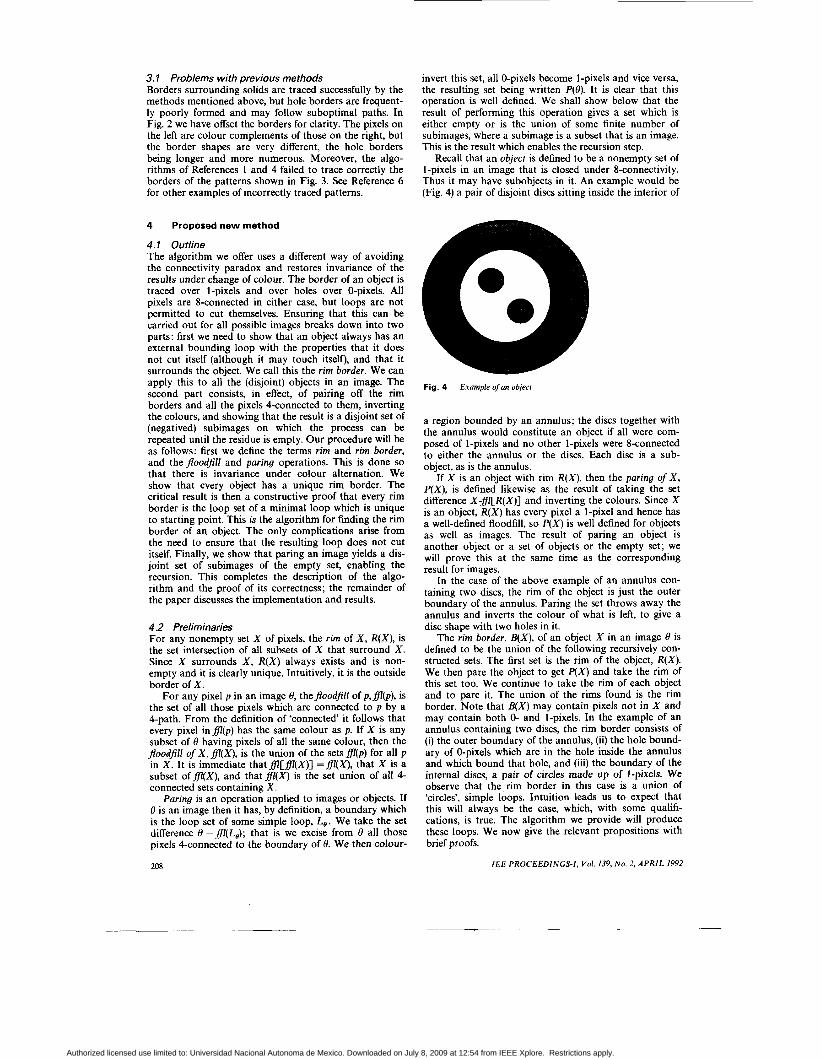
Recall that an object is defined to be a nonempty set of 1-pixels in an image that is closed under 8-connectivity. Thus it may have subobjects in it. An example would be (Fig. 4) a pair of disjoint discs sitting inside the interior of

Fig. 4 Example ofan object

a region bounded by an annulus; the discs together with the annulus would constitute an object if all were com- posed of 1-pixels and no other 1-pixels were 8-connected to either the annulus or the discs. Each disc is a sub- object, as is the annulus.

If X is an object with rim R(X) , then the paring of X, P(X) , is defined likewise as the result of taking the set difference X - f l [ R ( X ) ] and inverting the colours. Since X is an object, R ( X ) has every pixel a 1-pixel and hence has a well-defined floodfill, so P ( X ) is well defined for objects as well as images. The result of paring an object is another object or a set of objects or the empty set; we will prove this at the same time as the corresponding result for images.

In the case of the above example of an annulus con- taining two discs, the rim of the object is just the outer boundary of the annulus. Paring the set throws away the annulus and inverts the colour of what is left, to give a disc shape with two holes in it.

The rim border, B(X), of an object X in an image 8 is defined to be the union of the following recursively con- structed sets. The first set is the rim of the object, R(X) . We then pare the object to get P ( X ) and take the rim of this set too. We continue to take the rim of each object and to pare it. The union of the rims found is the rim border. Note that B(X) may contain pixels not in X and may contain both 0- and I-pixels. In the example of an annulus containing two discs, the rim border consists of (i) the outer boundary of the annulus, (ii) the hole bound- ary of 0-pixels which are in the hole inside the annulus and which bound that hole, and (iii) the boundary of the internal discs, a pair of circles made up of 1-pixels. We observe that the rim border in this case is a union of ‘circles’, simple loops. Intuition leads us to expect that this will always be the case, which, with some qualifi- cations, is true. The algorithm we provide will produce these loops. We now give the relevant propositions with brief proofs.

IEE PROCEEDINGS-I, Vol. 139, No . 2, A P R I L 1992

Authorized licensed use limited to: Universidad Nacional Autonoma de Mexico. Downloaded on July 8, 2009 at 12:54 from IEEE Xplore. Restrictions apply.

4.3 Justifying propositions Proposition I : If p is in the rim of an object X, then there is a 4-path from p to the boundary of the image which intersects X only in p.

Proof: Suppose every path from p to the boundary of the image intersects the rim in some pixel other than p. Then p may be removed from the rim, and it is still true that every pixel of X is surrounded by the new reduced set. But this contradicts the minimality of the rim.

Proposition 2: If a pixel p is in the rim of an object X and has any 8-neighbours also in X, at least one of them is also in the rim.

Proof: Suppose p and q are 8-adjacent pixels of X ; p is in the rim and q is not. By Proposition 1 there is a 4-path from p to the boundary which intersects X only in p. It must pass through one of the 4-neighbours of p ; without loss of generality, suppose it passes through location 0 relative to p. Then q is not in location 0 else there is a 4-path from q to the boundary of the image which inter- sects X only in q and hence q is not surrounded by the rim; a contradiction. In any other location, there are two possible 4-paths to the pixel 0 relative to p, which go around p , remaining 8-adjacent to p, and both of these must encounter a pixel of X which is 8-adjacent to p , and is in the rim of X, or q is not surrounded by the rim.

The following proposition has as (constructive) proof the border-tracing algorithm which is the core of this paper.

4.4 Border- following algorithm Proposition 3 : The rim of any object X in an image 0 is the loop set of some minimal simple loop which is unique up to starting point.

Proof: The image boundary can be expressed, by hypoth- esis, as a simple loop which may be taken to be minimal and traced anticlockwise. We may suppose that it has been constructed by some such process as using a point- ing device to generate the loop from some larger image. In generating such a loop, we start at some pixel and move onto another which is 8-connected to the first; if at some stage k we next move to a pixel p r + l which is already in the path set so far constructed, F say, we are constrained to ensure that we do not cut F; i.e. we must leave p by a pixel p k + 2 which does not have a pixel already traced lying between our consecutive pixels pr , pkc l , p k + 2 in the ordering of the 8-neighbours of p. Since simplicity is a local condition, we may make this check algorithmically without difficulty; it is, of course, a simple enough task for the human eye.

Constructing such a simple loop allows us to find 0- pixels which are topmost in the boundary of the image, i.e. no pixel in the loop is higher in the raster scan. We record the y-coordinate of a topmost pixel. Of these pixels we can find the leftmost (i.e. none of the topmost pixels are further left than this pixel) which is clearly unique. We also need to have the values of the x- coordinate of the leftmost and rightmost pixels and the y-coordinate of the downmost pixels, effectively putting a rectangular box around the image. We shall start scan- ning the image from this leftmost of the topmost pixels in the usual raster, left to right then move down, and scan. Horizontal scans require us to check right across the whole image until the x-coordinate is equal to that of some rightmost pixel; simply encountering the bounding

IEE PROCEEDINGS-I, Vol. 139, No. 2, APRIL 1992

loop is not enough reason a stop since there may be other pixels to the right.

To move down, we simply take the pixel in the loop which follows the last starting point of a horizontal scan. This suffices to ensure that every pixel of the image is scanned: but suppose this is not the case. Then there is a pixel q in the image which has not been scanned, and we have at completion returned to our starting point and have covered every pixel in the bounding loop as the start of a horizontal scan. Take the horizontal line of pixels to the left of q. This cannot meet the bounding loop, which therefore does not surround the image; a contradiction.

In constructing the bounding loop, it is convenient to label the pixels of the loop as either searchable if an image pixel lies to the right of them or unsearchable if no such image pixel exists. We shall do the same for objects.

We can now start the search to find the objects of 8. The bounding loop is, by definition, a set of @pixels.

0 0 0 0 0 0 0

direction of ~

l inescan O O O 0

0 0 0 0 0 0 0 0 0

Fig. 5 Initial poim may be re-entered

Starting again at the leftmost of the topmost pixels of the bounding loop of 8, we scan until a 1-pixel is encohntered or we meet an unsearchable pixel. If a 1-pixel is encoun- tered, we enter a border-following procedure defined as follows.

We know that there is no 1-pixel of the object encoun- tered to the left of the current scan line. We therefore consider the ray which has its origin in this first I-pixel, p I , and extends to the left, and which intersects only 0- pixels except for p 1 itself. This ray is swept clockwise about p l until it encounters another 1-pixel which is an 8-neighbour of p 1 or returns to its starting position. Now p 1 must be in the rim of the object X containing it, and by Proposition 2 either it is the only pixel of X or the rotating ray will find an 8-neighbour of p 1 which is in X. The first such pixel is declared to be p 2 . We claim this is in the rim of X, and the argument is that of Proposition 2.

We now go to the inductive step. Suppose we have found a rim pixel of X, p k , for k > 1. Then we take the ray from pk back through pt - 1. This is swept clockwise until it encounters another 1-pixel; the first such pixel is declared to be p k I 1 . We observe that this process ensures that there is never another incoming pixel between an incoming pixel and an outgoing one, so if it defines a loop the loop must be simple. The termination condition has two parts: we must return to a pixel previously encountered in the path, thus giving a loop. This is not sufficient, however; we must continue tracing until the ray also returns to its original position or we may omit part of the object.

It is plain that the path must indeed return to its start- ing point and the ray to its original orientation even- tually, since there are only finitely many 1-pixels in the image, only eight possible orientations, and pr and pk+ I

are always distinct. It is also plain that the loop is minimal and contains only rim pixels. It yields the rim border of the object.

Having terminated the finding of the rim border of X (which is conveniently specified by its first pixel and a

209

Authorized licensed use limited to: Universidad Nacional Autonoma de Mexico. Downloaded on July 8, 2009 at 12:54 from IEEE Xplore. Restrictions apply.

since there'may be other objects to the right of the found object. The same procedure is implemented on encoun- tering another 1-pixel unless that pixel is one already in the rim border of an earlier object. This may be done conveniently by finding the topmost, leftmost, downmost and rightmost elements of the rim border of X and label- ling the pixels as searchable or unsearchable in the same sense as for the image, except that now we do it on 1- pixels.

On completing a horizontal scan by encountering an unsearchable boundary pixel, we return to the last pixel of the bounding loop of 8 used as a scan start, and take the next loop pixel to be our next scan start. A 1-pixel which is found may be checked to see if it is the bounding loop of a rim border found higher up; if so we jump all the 1-pixels until a 1-pixel in the boundary labelled as unsearchable is encountered, and then we restart the horizontal scan from the @pixel to its right. This ensures that we do not start tracing the rim border of objects entirely surrounded by the outer object. It is plain that this procedure will give a simple minimal loop which has loop-set the rim border of the object X; moreover, every such object X must be found by the scanning procedure which calls the border-following procedure for X. We observe that the objects are disjoint since they are closed under 8-connectivity.

4.5 The induction step Proposition 4 : The result of paring an image 8 is a set which is either empty or the finite union of disjoint images, and the result of paring an object is that it is empty or a finite union of disjoint objects.

Proof: To take the trivial case first, if an image contains no objects, then it must consist of only 0-pixels and paring it will yield the empty set. So we may take it that there is at least one object X in 8. Paring removes all the 0-pixels in the background, which leaves everything inside the rim border of the (disjoint) set of objects. Let H ( X ) denote the hull of the object X, i.e. the set of all pixels surrounded by the rim of X. Since the objects are closed under 8-connections, the complement of the union of the hulls is 4-connected and must therefore be the floodfill of the boundary of 8. Paring first removes this complement, giving a union of the hulls, which are also disjoint. Each hull is then colour-inverted. The rim of each hull is, by Proposition 3, the loop set of a simple minimal loop and is hence an image.

If X is an object, the same argument holds by colour inversion.

Proposition 5: The rim border of an object in an image suffices to reconstruct the object.

Proof: Recall that the rim border is constructed by taking the union of the rim of an object, then paring and taking the rim of the result, which process is iterated until the result is empty. This yields a set of chain codes for the rim loops and some pixels on each such loop, the colours of the pixels alternating as we move into the object and its holes. To reconstruct the object, we start with the out- ermost loop and floodfill with the loop's colour. The only obstruction is any internal loop, which is precisely the rim border of a hole. Clearly all the floodfilled pixels return to the correct colour. This is now iterated with the appropriate colour change from the rim border of the holes.

210

5.1 Effect of the new definition The images of Fig. 2, may be compared with those of Fig. 6, which were obtained using the new definition. The improvements may be seen to include the following:

(1) There are fewer hole borders in some cases, resulting in better data compression and faster processing in later stages.

(2) Colour inversion produces the same chain code. (3) Hole borders are shorter, again resulting in better

compression and less postprocessing.

These improvements can also be achieved for three- dimensional images [S-81.

0 0 0 0 0 e e m e m

0 e 0 0 0 0 0 e e e e e

a b

0 0 0 0 0 e e e e m

o o o o o e e e e e C d

Fig. 6 a. b Length = 9 e. d Length = 4

Hole shape is improved (cf Fig. 2)

5.2 Implementation 5.2.1 Border-tracing algorithm: This is readily imple- mented as a pair of co-recursive procedures. It does not require the image border to be rectangular, although it may require a frame of 0-pixels to be placed around the initial image. The object search and the image search are identical except for colour inversion.

52.2 Coding: The algorithm requires a frame buffer of 3-bit planes to store the list of searchable and unsearch- able pixels and to extract the topological information to

Fig. 7 Topology of image

arbitrary depth. This compares favourably with those methods where the depth of the buffer depends on the number of loops used. The algorithm has been coded in C and comprises about 150 lines.

5.3 Results The method has been tested extensively on artificial and biomedical images. It correctly locates and traces all the borders shown in Fig. 3 that were incorrectly traced by the previous methods. It may be seen that the hole borders are better shaped and more compact.

IEE PROCEEDINGS-I, Vol. 139, No. 2, APRIL I992

Authorized licensed use limited to: Universidad Nacional Autonoma de Mexico. Downloaded on July 8, 2009 at 12:54 from IEEE Xplore. Restrictions apply.

6 Acknowledgments

The authors wish to express their gratitude to Mr. Ian Morris of the Queen Elizabeth Medical Centre for sup- plying the magnetic resonance images used in this work. We also wish to thank Mr. Khanh Ly for valuable dis- cussions and providing code for other algorithms used for comparisons. This work was supported by an Aus- tralian Commonwealth Postgraduate Research Award, and by a research grant from The University of Western Australia.

7 References

1 ROSENFELD, A., and KAK, A.C.: ‘Digital picture processing’ (Academic Press, New York, 1982,2nd edn.), Vol. 2

IEE PROCEEDINGS-I, Vol. 139, No . 2, APRIL 1992

2 PAVLIDIS, T.: ‘Algorithms for graphics and image processing’ (Springer-Verlag, Computer Science Press, MD, 1982)

3 SUZUKI, S., and ABE, K.: ‘Topological structural analysis of digital binary image by border following’, Comput. Graphics Image Process., 1985,Jo. pp. 32-46

4 LY, K., and AlTIKIOUZEL, Y.: ‘Contour tracing of biomedical binary images’, Proc. Int. Symp. Signal Process., 1987,2, pp. 735-739

5 KRUSE, B.: ‘A fast stack-based algorithm for region extraction in binary and nonbinary images’ in ‘Signal processing theories and applications’ (North-Holland Publishing Co., Amsterdam, 1980)

6 DANIELSSON, P.-E.: ‘An improved segmentation and coding algo- rithm for binary and nonbinary images’, IBM J. Res. Den, 1982, 26, pp. 698-707

7 TORIWAKI, J . 4 , and YOKOI, S.: ‘Algorithms for skeletonizing three dimensional digitized binary pictures’, Proc. SPIE, 1983, 435, pp. 2-91

8 CHEN, B.-D., and SIY, P.: ‘Forward/backward contour tracing with feedback’, IEEE Trans., 1987, PAMI-9, (3), pp. 438-446

211

Authorized licensed use limited to: Universidad Nacional Autonoma de Mexico. Downloaded on July 8, 2009 at 12:54 from IEEE Xplore. Restrictions apply.