WP 13/27

Born to Win? The Role of Circumstances and Luck in

Early Childhood Health Inequalities

David Madden

August 2013

york.ac.uk/res/herc/hedgwp

Born to Win? The Role of Circumstancesand Luck in Early Childhood Health

Inequalities

David Madden

(University College Dublin)

August 2013

Abstract: This paper measures the degree of inequality of opportunity in

birthweight and birthlength for a sample of Irish infants. The sample is partitioned

into eight types by mothers’ education and mothers’ smoking status. Stochastic

dominance tests reveal the presence of inequality of opportunity but its fraction of

total inequality is comparatively small at 1-2%, with the remainder of inequality

assigned to random, unobserved factors. These results are robust to finer

partitioning of the population and to re-definition of types’ opportunity sets which

gives greater weight to inequality at the lower end of the distribution. Analysis of

the incidence of low birthweight and short birthlength using measures from the

poverty and segregation literature also reveal that incidence is not uniform across

type and is consistent with the presence of inequality of opportunity.

Keywords: Inequality of opportunity, decomposition, poverty, child health

JEL Codes: I14, I24, J13.

Corresponding Author: David Madden,

School of Economics,

University College Dublin,

Belfield,

Dublin 4,

Ireland.

Phone: 353-1-7168396

Fax: 353-1-2830068

E-Mail: david.madden@ucd.ie

Born to Lose? The Role of Circumstances and Luck in Early

Childhood Health Inequalities

1. Introduction

There is now a fairly wide body of evidence that health inequalities and deprivations which

are experienced in very early childhood can have long lasting effects. This includes not just

effects on subsequent health, but also effects on other outcomes such as education and

earnings (for example see Almond and Currie, 2011a, 2011b, Black et al., 2007, Currie, 2011

and for evidence for Ireland, Delaney et al, 2011). One of the most frequently studied early

childhood health outcomes is birthweight. There is evidence that low birthweight is

associated with adult mortality, especially cardiovascular mortality (see Risnes et al, 2011),

and also evidence that low birthweight is concentrated among lower income groups (see

Kramer et al 2000, and for evidence for Ireland see, Madden, 2013, McAvoy et al 2006,

McGovern, 2011 and Niedhammer et al 2011). Recent research by Figlio et al (2013)

suggest that the gaps observed in adulthood arising from low birthweight become established

at very early ages, perhaps even as low as kindergarden, indicating that “...some biological

factors may be very difficult to overcome”. Associations have also been found between birth

length and adult mortality (Nybo Andersen and Osler, 2004).

The evidence cited above indicates that analysis of childhood health inequalities in such

outcomes, as well as providing insights into childhood mortality and morbidities, may also be

of use in combating adverse health and labour market outcomes for adults. Patterns of

inequality which are found in childhood health may be reproduced in adulthood. Thus

analysis of the extent and nature of inequality in childhood health outcomes may be an

important input into research into a variety of both childhood and adult outcomes.

Much of the recent literature in the analysis of (in)equality has concentrated upon equality of

opportunity, as opposed to equality of outcome and this has also been the case in the area of

health economics (e.g. Dworkin, 1981, Rosa Dias and Jones, 2007). While the precise

definitions of equality of opportunity may differ, in all cases a clear distinction is made

between what may be regarded as “fair” and “unfair” sources of inequality. In some cases

the terms ethically defensible and indefensible have been used. For example, what are

sometimes labelled as ”circumstances” such as genetic endowments and parental socio-

economic outcomes are seen as unfair sources of inequality, whereas inequality arising from

factors such as effort or lifestyles may be seen as fair.

A formal framework for this view of equality was established by Romer (1998, 2002). For a

given health outcome for an individual hi we divide all factors which might affect this

outcome into effort factors and circumstance factors, bearing in mind that some effort factors

themselves may depend upon circumstances e.g. the amount of care/effort someone puts into

their diet may be affected by the dietary habits of their parents. The Romer model does not

specify which factors could be considered as effort and which as circumstance and clearly

there is considerable room for debate here. There may also be purely random factors which

affect health outcomes in the sense that once all effort and circumstance factors have been

accounted for there will still be a residual degree of inequality in the health outcome.

In this paper we try to identify factors which affect early childhood outcomes and which can

be clearly regarded as circumstances. The outcomes we choose are birthweight and

birthlength. Note that since we are analysing an outcome at birth, we do not need to dwell

on the circumstance/effort distinction, since it is entirely unreasonable to expect an infant to

consciously exert effort. Thus our analysis will concentrate entirely upon inequality arising

from differential circumstance, plus whatever residual inequality is left.

The Romer model partitions the population into different types, whereby a type consists of

individuals who are exposed to the same set of circumstances and the number of types should

be mutually exclusive and exhaustive. The precise number of types is left to the choice of the

analyst but the types should be meaningful in the sense that each should have a sufficiently

different set of circumstances so that they can be realistically regarded as providing a

different opportunity set for each type. From a purely practical point of view there may also

be an upper limit on the number of types. Too fine a partition will lead to types containing

only a small number of individuals and these small cell sizes may inhibit statistically

significant comparisons between types. The range and number of types will also clearly be

constrained by data availability. In our application here we partition the population along

two dimensions, education of mother and smoking status of mother. We define four

categories of education and two categories of smoking, thus giving us eight types in total.

Equality of opportunity then dictates that average health outcomes should be identical for

each type, for given levels of effort.

For models where effort is relevant, then what is known as the Romer identification

assumption deems that two individuals (from different types) are reckoned to have exerted

the same effort if they are located at the same percentile of their type’s distribution of effort.

Even if effort is not directly observable then an additional assumption of a monotonic

relationship between effort and the health outcome implies that individuals (from different

types) located at the same percentile of the health outcome are considered to have exerted the

same effort. However, as we explained above, given that we are looking at outcomes in very

early childhood, effort is not relevant.

Given this framework for analysing inequality of opportunity, there are a number of different

ways to proceed. First of all, in section 2 we will examine stochastic dominance in the health

outcomes between different types. The presence of stochastic dominance is sufficient to

illustrate the presence of inequality of opportunity. In section 3 we will attempt to measure

the degree of inequality of opportunity in our health outcomes, while in section 4 we carry

out some sensitivity tests. In section 5 we change the focus slightly and examine the

incidence of low birthweight and birthlength across different sets of circumstances while

section 6 provides discussion and concluding comments.

2. Detecting Inequality of Opportunity: Stochastic Dominance

Stochastic dominance provides a means for testing for the presence of inequality of

opportunity, but it does not provide a direct measure of such inequality. First order stochastic

dominance (FSD) applies to all utility functions u(.) whereby 0(.) u and involves

comparison of the cumulative distribution functions (cdf) of whatever is the argument of the

utility function e.g. income, health etc. Second order stochastic dominance applies to utility

functions which are increasing and concave, 0(.) u and 0(.) u and involves the

comparison of the integrals of the cdfs. Alternatively, second order stochastic dominance is

relevant when agents are risk-averse. Lefranc et al (2008) discuss which dominance concept

should apply under different circumstances. They suggest that in a purely deterministic

world, where outcomes are the product of circumstances and effort, and where individuals

know their level of effort, then FSD is appropriate. However, where luck is involved, or

where it is difficult to disentangle the effects of effort and luck and hence where the outcome

is uncertain, even when circumstances are known, then SSD is appropriate. In our example,

here, while it does not seem reasonable to regard effort as relevant, there clearly is a role for

random factors (which we can call “luck”) and in that case SSD seems most appropriate.

A comparison of the cdfs for different types can be used to detect the presence of inequality

of opportunity. If we denote type, or circumstance, by c and the cdf for our health outcome

by F(.) then inequality of opportunity is present if for any )(., cFcc >SSD )(.cF and >SSD

refers to second order stochastic dominance. Thus we need to compare the integrals of the

cdfs for the different types to check if second-order stochastic dominance holds in any

bilateral comparison.

Before testing for stochastic dominance we first give some details concerning our data.

The data comes from the Growing Up in Ireland (GUI) survey, 9 month old infant cohort,

wave 1 (for a summary guide to this survey see Quail et al, 2011). The 9 month cohort

comprised 11134 children born between 1st December 2007 and 30th June 2008. The

sampling frame was drawn from the Child Benefit Register. Child Benefit is a payment made

with respect to all children aged 16 years or under, and has many features which render it an

ideal sampling frame for this exercise (see Quail et al, 2011, for details). The sampling

weights provided are used to further ensure that the sample is representative.

The two health outcome measures which we analyse are birthweight and birthlength.

Birthweight is recorded in the survey in intervals of 100 grams and there is data censoring at

both the top and bottom of the distribution. All birthweights in excess of 4600 grams are

listed as 4600. Meanwhile all birthweights below 1499 grams are listed as 1499. In addition

birthweights in the 1500-2499 interval are simply listed as 2499. 0.74% of observations are

below 1499 grams, 4.86% are in the 1500-2499 interval while 2.2% are above 4600 grams.

To remove some of the censoring of the data for the 1500-2499 interval we used data from

the 2009 perinatal statistics to interpolate birthweights for the <1499 and 1500-2499

intervals. On that basis, birthweights for these intervals are set at 1066 and 2127gms

respectively. Overall, however, the censoring of the data at top and bottom and its

presentation in interval form will reduce recorded inequality.

Birthlength is recorded in centimetres. Once again there is some censoring of the data and

some presentation in interval form. Babies with length less than 29cm are listed as 29cm.

Length is then listed in intervals of 30-39 and 40-45cms. It is listed in one cm intervals up to

57cm and then in intervals of 58-59cm, 60-64cm and >65cm. 1.81% of babies are less than

29cm and 1.72% are greater than 65cm. For the case of babies whose length is listed in

intervals we assume that the distribution of length within these intervals is uniform and so we

use the mid-point of the interval.

We two sets of circumstances which in total provide us with eight types. The first set of

circumstances is the highest level of education completed by the mother. We divide this into

four types. Type 1 consists of those mothers who have not completed secondary school

education. Type 2 consists of mothers who highest level of education is the Leaving

Certificate (or equivalent). The Leaving Certificate is the standard exam which all Irish

students undertake on completion of second level schooling. Type 3 consists of mothers who

complete a post Leaving Certificate diploma or certificate but do not take a university degree.

Finally, type 4 consists of mothers who have completed a primary degree (this type also

includes those with a postgraduate degree). The second circumstance we use is current

smoking status. Respondents who answer “yes” to the question “do you currently smoke

daily?” are deemed as smokers.

Of the original sample of 11096 singleton births where the survey is completed by the birth

mother, there are 127 observations with missing birthweight data. More problematically

there are 5695 observations with birthlength data missing. The missing observations for

birthlength do not appear to be at random. For example, a two-sample t test for equality of

birthweight between those where birthlength data is missing and those where it is present, has

a t statistic of over 11 and a p-value of 0.000. Thus in the results which follow we will

present inequality results for birthweight for the complete sample and also for the sample

where only data on both birthweight and length are available.

In tables 1 and 1A we present some summary statistics for the smaller and larger samples.

We can see straightaway that cell sizes (i.e. types) are far from uniform in size. In particular

types which include smokers are generally smaller, reflecting the fact that smokers are a

minority amongst mothers. Our sample has smoking rates of 15-17 percent, depending upon

whether the larger or smaller sample is used. This is below the overall smoking rate for

women of child-bearing age (see Brugha et al, 2009), but of course this overall rate also

includes non-mothers. Comparing tables 1 and 1A, we also see that within the smaller

sample, there is a higher proportional representation amongst the better educated (for both

smokers and non-smokers).

In table 2 we present results for pairwise tests between types of second order stochastic

dominance for birthweight. The results are presented in the form of a grid which shows

whether dominance applies. The table should be interpreted as indicating whether the row

type dominates the column type, whereby dominance indicates that the integral of the

cumulative frequency for the column type for each birthweight (as we go from lower to

higher) is always higher than the integral of the cumulative frequency for the row type. We

denote dominance by an entry of “>” and this indicates that the difference was statistically

significant. This also covers the situation where the difference between the integrals of cdfs

was not statistically significant over some part of our birthweight range, but that it was

statistically significant over another part. We do not observe dominance if either there is no

part of the birthweight range where there is a statistically significant difference or if over the

range we observe two (or more) instances of a statistically significant difference but of

opposite sign. In carrying out this analysis we used the Distributive Analysis Stata Package,

DASP, kindly provided by Arrar and Duclos (2012).

What overall message can be drawn from table 2? Firstly, the presence of second order

stochastic dominance indicates that inequality of opportunity is present. Note also that the

majority of “>” entries are in columns corresponding to smokers i.e. it is smokers who are

dominated. This indicates that smoking status seems to be the most important circumstance

in terms of inequality of opportunity. In one case a non-smoking type with lower education

attainment dominates a smoking type with higher educational attainment i.e. non-smokers

who have not completed secondary school education dominate smokers who have completed

secondary education.

To summarise, it is clear from the presence of second order dominance in many of the

pairwise comparisons that inequality of opportunity is present. It is also clear that in terms of

the types we have identified, the circumstance which appears to “matters most” is smoking.

Within categories of education, non-smokers almost always dominate smokers (the exception

is Diploma/Cert). Non-smokers always dominate smokers of lower education, and in one

case even dominate smokers of a higher education level.

Do these results carry through when we use the larger sample? By and large the answer is

yes and given that we have a larger sample we have considerably more “>” entries. Once

again, smoking is the critical factor with most of the “>” entries in the columns of smokers.

We observe again that non-smokers can dominate smokers of higher education, with 3rd level

smokers in particular dominated by non-smokers from lower educational types. Within the

category of smokers, it is only for those who failed to complete second level education that

education matters. Within the category of non-smokers, it is only those who have completed

the Leaving Cert who are dominated by higher educated types.

What about birth length, our other child health measure? Table 3 shows the same grid as

tables 2 and 2A, bearing in mind that we are dealing with the smaller sample here, so

statistical significance is more difficult to establish. In general, we see fewer cases of

dominance, with the exception of smokers who have not completed second level education.

This group is dominated by all others. The other instances where we see dominance are

where 3rd level non-smokers dominate nearly all other types, apart from 3rd level smokers.

We can summarise the results of this section as follows: analysis of second order stochastic

dominance in birthweight for pairwise comparisons of our eight different types provide fairly

conclusive evidence of inequality of opportunity, in that many of the comparisons reveal such

dominance. Smoking status appears to be the key characteristic, more so than education.

With respect to birthlength, there is less evidence of dominance and hence of inequality of

opportunity. However, outcomes for smokers who have not completed second level

education are dominated by outcomes for other groups, indicating that this type, at least,

experiences inequality of opportunity. It is also the case that 3rd level non-smokers dominate

the other groups, so once again this is evidence for inequality of opportunity.

Having confirmed the presence of inequality of opportunity in our data, we now attempt to

measure it.

3. Measuring Inequality of Opportunity

There are a variety of approaches which can be taken to measuring inequality of opportunity

and a recent comprehensive survey can be found in Ramos and Van de gaer (2012). What

they term the direct way of measuring Inequality of Opportunity is to estimate the degree of

inequality in a counterfactual distribution where inequalities due to effort have been removed

and what remains is simply inequality arising from circumstances. Thus given the health

outcome hi, we wish to measure I(hf) where hf represents counterfactual health, whereby

inequalities due to differences in effort or luck have been eliminated. There are then two

critical decisions to be taken: the choice of hf and the choice of the specific inequality index I.

We consider two non-parametric approaches to hf. In the first case the health outcome for

each individual is replaced by the average health outcome for his type. Thus we have

cNi

i

c

fc h

Nh

11 where Nc refers to the number of people in type c.

Before considering the second non-parametric approach, we discuss the choice of inequality

index. Van de gaer proposed an inequality index with infinite inequality aversion, on the

basis that all inequality arising from circumstances is morally objectionable. Checci and

Pergaine (2010) and Ferreira and Gignoux (2011) on the other hand prefer the use of the

mean log deviation (also known as the Theil (0) measure), since this measure has the

advantage of being both decomposable and path independent. The expression for this is

N

i ih

h

NMLD

1

ln1

where h is the average health outcome and we have suppressed the

notation for “type” for convenience. When 1fch is employed, then total health inequality

decomposes exactly into )( 1fchI and a counterfactual where all types have an opportunity set

of the same value ).(1f

c

ih

hhI .

The second non-parametric approach is that of Lefranc et al (2008) who propose what they

term the Gini Opportunity index (GO). The intuition behind this is that if we label the Gini

index for the health outcome for each type as Gc then the opportunity set for each type is

given by )1( cc Gh where ch is the average health outcome for type c. Thus

)1(2cc

fc Ghh and once again, applying the mean log deviation measure overall inequality

will decompose exactly into )( 2fchI and a counterfactual where all types have an opportunity

set of the same value ).(2f

c

ih

hhI .

It should be noted that the above approaches fall within the category labelled as the

“utilitarian ex ante (types)” approach by Checci and Peragine (2010). They also suggest an

“ex post (tranches)” approach whereby each tranche represents a given level of effort. In

general, it is useful to look at both approaches and to compare the results. However, since it

simply does not make sense to speak in terms of effort for our application here, we restrict

ourselves to the ex ante approach.

It is also worth noting that Lefranc et al do not use the mean log deviation measure but

instead suggest measuring ex-ante inequality by calculating the Gini coefficient for 2fch .

Thus if we index types from 1...k and order types in increasing order by 2fch the GO index is

then given by

k

i ji

fci

fcjji hhpp

hGO ][

1 2,

2, and pi refers to the sample weight for type i.

Effectively what they are doing is to construct a form of Gini index over types’ opportunity

sets.

Lefranc et al also show that it is possible to decompose their GO index into a risk and return

component. Since the opportunity set is the product of average health for each type and the

Gini within each type, the overall GO index will comprise a part arising purely from

differences in return, and a part arising from differences in risk. To isolate the part arising

from return only we assume that all within type risk is eliminated, leaving us with the

following expression:

k

i jiijjipt hhpp

hGO ][

1.

The pure risk component is then obtained by assuming that between type inequality of health

outcome is eliminated, leaving us with the expression:

k

i jijijipr GGpp

hGO ][

1.

Note that the ranking which is used in the construction of these two terms is the same ranking

as used in the overall GO index and because of this it is possible that one or other of GOpt or

GOpr may be negative. It is also the case that the decomposition will not be exact, as is

typically the case with Gini based decompositions. Hence there will be a residual interaction

term:

k

i jijjiijiprpt hhGhhGpp

hGOGOGO )]()([

1.

In general the expectation is that the ranking by average health will be highly correlated with

that by health opportunities and so GOpt is unlikely to be negative. However if it is the case

that health riskiness is greater for healthier types then GOpr may be negative. Thus the sign

of GOpr is a useful summary of the correlation between risk and return by type.

Table 4 provides results for the decomposition of overall inequality of our health outcomes

into that arising from inequality of opportunity (essentially inequality between types, once

within type inequality has been eliminated) and that arising from inequality within types

(when between type inequality has been removed). We provide results for both health

counterfactuals (average health for each type and the health opportunity set for each type).

The qualitative results are very similar. First note that overall inequality is greatest for

birthweight with the larger sample and inequality for birthlength is only about 50-60% of that

for birthweight. This is consistent with the extent of “>” entries in tables 2 and 3.

The second feature of table 4 is that inequality of opportunity (in the sense of inequality

between types) is only a small fraction of overall inequality, typically in the region of 1-2%.

By far the greatest contribution to inequality comes from within-type inequality. In other

applications of this analysis such inequality would be regarded as inequality arising from

different effort. However, as it is not realistic to think of effort in this application it must be

concluded that the bulk of inequality is arising from random factors or “luck”. This result

holds regardless of which counterfactual measure of birthweight/length is used, although

inequality of opportunity is slightly higher when 2fch is used.

Of course, this is conditional upon mothers education and smoking status being the only

relevant circumstances. It is highly likely that there are omitted circumstances and their

contribution to overall inequality is being classified under luck or random factors. Thus our

estimate of inequality of opportunity should be seen as a lower bound. Given the approach

we take here to measuring inequality of opportunity, the inclusion of extra circumstances

would come at the cost of increasing the number of types and hence create problems with

small cell sizes etc.

Table 5 gives the results for the GO index of Lefranc et al. Note that we cannot compare the

values of the indices in tables 4 and 5, since in table 4 inequality is measured via the mean

log deviation, whereas in table 5 it is measured by a Gini type index. Once again, inequality

of opportunity is greater for birthweight than for birthlength, but this time it is slightly higher

for the smaller sample. In terms of the decomposition into pure risk and pure return, by far

the larger contribution comes from pure return, indicating that inequality in the health

opportunity sets arises primarily from differences in the average health outcome by type, as

opposed to differences in the level of inequality within each type. It is also worth noting that

the values of the GO index obtained in table 5 are qualitatively similar to those obtained in

Rosa Dias (2009), although he was looking at overall adult self-assessed health.

Finally, we note that the values of GOpr which we obtain are very small, indicating very little

correlation between risk and return by type.

The results from table 4 are perhaps surprising. Given that tables 2 and 2A indicated that

inequality of opportunity was present, the extent of such inequality, as measured by table 4,

seems modest. In the next section, we try to explore this and examine the sensitivity of our

results to some of the assumptions we have made.

4. Discussion and Sensitivity Checks

In this section we explore our results to see if they are robust to a number of changes in

specification. In particular, we choose to extend the analysis in three directions (in the

examples which follow we provide results for birthweight only for the larger sample – results

for other measures are available on request).

First of all, we use a different counterfactual distribution of health, hf, one which uses the

concept of health opportunity sets as with 2fch above, but where a greater weight is placed

upon inequality at the lower end of the distribution. In many ways, this perhaps comes closer

to what we are ideally trying to measure, since the health consequences of inequality at the

upper end of the birthweight distribution are presumably less serious than at the lower end

(see for example the results in Nybo Andersen et al, where relative risk ratios fall quite

sharply as birthweight moves from <2500gms to the 2500-3400gms interval).

Recall that in our measure 2fch above that we defined the opportunity set for each type as

)1(2cc

fc Ghh i.e. average health for each type times one minus the Gini coefficient for

health within that type. This uses what we can regard as the “standard” Gini coefficient.

However it is also possible to use the extended Gini coefficient of Donaldson and Weymark

(1980). The Gini coefficient can be thought of as the sum of the distance between the line of

perfect equality and the Lorenz curve. For the standard Gini the distance for each percentile

is given the same weight. However it is also possible to introduce percentile dependent

weights, along the lines of κ(p; ν)=ν(ν-1)(1-p)ν-1. By altering the parameter v we can change

the weight placed on the lower part of the distribution (the case of the standard Gini is where

v=2) whereby a higher value corresponds to a higher weighting on inequalitires at the lower

end of the distribution. We choose a value of v=5 and calculate a new health counterfactual

))5(1(3 vGhh ccf

c . We then apply the mean log deviation measure of overall inequality

again, which will decompose exactly into )( 3fchI and the counterfactual where all types have

an opportunity set of the same value ).(3f

c

ih

hhI .

The second direction in which we extend the analysis is to increase the number of types. It is

possible that our partitioning of the sample into eight distinct types (by education and

smoking status) is not fine enough. Thus we introduce a further partitioning, this time by

self-assessed health. All mothers provide a response to the question: in general, how would

you say your current health is? There are five possible responses: excellent, very good, good,

fair and poor. We convert this into a binary response with two heath types, those who

respond excellent or very good (about 70% of the sample) and the rest. This further

partitioning gives us in total sixteen different types, the eight we have used so far which are

further repartitioned into two health types.

Tables 6 and 7 gives the results for these “sensitivity” tests. We first of all present results

using 3fch with the original eight types. We then present results for 1f

ch , 2fch and 3f

ch using

sixteen types. The results are extremely similar to those in table 4. Both changes lead to

marginal increases in measured inequality of opportunity, but even when we combine the two

changes, with the case of 3fch with sixteen types, inequality of opportunity still only accounts

for just over 5% of total inequality. The vast majority of inequality still arises from

inequality within each type. We also carried out the same analysis using income quartiles

rather than education and the results were qualitatively similar (results available on request).

Are the results presented here consistent with other results concerning the socioeconomic

gradient of low birthweight? Studies cited in the introduction to this paper indicate a fairly

consistent pattern of low birthweight being predominantly concentrated amongst lower

income groups (or types), yet the results here suggest that when looking at overall

birthweight, inequality by type is not pronounced, even when using an inequality measure

which places a high weight on inequality at the bottom of the distribution. Perhaps the

solution to this apparent contradiction is that other studies have examined the incidence of

low birthweight (i.e. births less than 2500 gms) as opposed to this study which has looked at

inequality over the complete distribution of birthweight.

Concentration upon the incidence of low birthweight (and birthlength) is more akin to

economic studies of poverty whereby there is a focus on those observations below a certain

key threshold. In the case of standard income poverty analysis the focus is upon those below

the poverty line. Here, however, the focus is upon those below the relevant low birthweight

and birthlength thresholds. As will be discussed below, given the nature of poverty indices it

is not possible to directly translate the inequality of opportunity analysis over to the case of

poverty. Nevertheless it is still possible to decompose such indices on the basis of type and

to assess the contribution of each type to the overall incidence of low birthweight/birthlength.

It is also possible to construct summary indices which indicate the degree to which the

incidence of low birthweight/birthlength is not uniform across type. This is the focus of the

next section.

5. The Poverty of Low Birthweight and Birthlength

The results above indicated that there was relatively little inequality in birthweight between

types. In terms of total inequality, it accounted for only about 1-2%, with the remainder

being assigned to within-type inequality. It was commented that this appeared strange, given

that the results of the stochastic dominance analysis indicated the presence of inequality of

opportunity (i.e. inequality between type). It also appears to be at odds with other results

which indicate the presence of socioeconomic inequality in low birthweight (Madden, 2013).

One reason for this anomaly is that the analysis in section 3 examines inequality across the

whole of the birthweight distribution. However, it is arguable that it is inequality at the lower

end of this distribution which should be of concern to us. In section 4 we tried to overcome

this by redefining the opportunity sets of each type as being average birthweight times one

minus the extended Gini. This will tend to lower the opportunity sets for types where there is

greater inequality at the lower end of the birthweight distribution and should increase the

spread between types. However, the change in measured inequality of opportunity was

relatively marginal.

In this section, we take a different approach, albeit at the cost of abandoning to some degree

the framework of inequality of opportunity. In the immediate exposition which follows we

use birthweight as our example, and we subsequently apply the analysis to birthlength also.

We use the standard 2500 gms threshold for low birthweight and thus we can regard it as our

“poverty line”. We analyse low birthweight by type via the group-wise decomposition of the

well-known Foster-Greer-Thorbeck (FGT) Pα poverty index. The formal expression for this

index is:

H

i h

ih

z

hz

NP

1

1where zh is the low birthweight threshold, hi refers to

birthweight of observation i, H is the total number of observations below the threshold and N

is the total number of observations. The parameter α represents the weight placed on each

proportionate “poverty gap”. When α=0, the poverty measure collapses into the headcount

index i.e. the fraction of the sample below the threshold. When α=1, then we have the sum

of proportional poverty gaps and when α=2 we have the sum of squared proportional gaps,

whereby inequality amongst those below the threshold is taken into account.

For our analysis in this section, we concentrate upon the case where α=0, since as explained

in the data section above, there is censoring of the data for some of the very low birthweight

observations, and hence it is not possible to obtain an accurate measure of birthweight (and

hence of the gap between birthweight and the 2500 gms threshold) which is needed for the

cases where α≥1.

The FGT measure has the convenient property that, given k mutually exclusive and

exhaustive groups, total poverty is equal to the weighted sum of the FGT measure for each

sub-group, where the weights are provided by each group’s share of the sample. Table 7

provides the groupwise decomposition of low birthweight for our sample. The table shows

the rate of low birthweight for each type, the population share of each type and the absolute

and relative contribution of each type to overall birthweight. The final column shows the

relative risk of low birthweight for each type. If low birthweight was distributed uniformly

across the population then this column would consist simply of “ones”. However, as is clear

from the column, the relative risk is not uniform across types and it is highest in the smoking

groups (the odd numbered types) and is highest of all for smokers with the minimum level of

education. The qualitative pattern is the same for both large and small samples.

What about birthlength? There is less consensus concerning the appropriate threshold for

short birthlength. We chose a threshold of 40cm. While this is to some extent arbitrary, the

same criticism could be made for pretty much any length which was chosen. The value of 40

is chosen as it approximates to being two standard deviations below the mean, a rule-of-

thumb suggested in Saenger et al (2007). The decomposition is in table 8 and once again an

effect of education and smoking status is evident. However, unlike the case with birthweight,

non-smoking observations with lower education (types 2 and 4) have a higher relative risk.

The relative risk for the highest educated smokers (type 7) while higher than their non-

smoking counterparts is not as high as is the case with birthweight. A further notable feature

of the birthlength data is that the relative penalty and advantage attached to the two

“outlying” types (the least educated smokers and the best educated non-smokers) respectively

are greater in the case of birthlength compared to birthweight.

In table 9 we also present a version of tables 7 and 8 for a group which can be termed as

“small for gestational age” or SGA. These are infants who are either low birthweight and/or

short birthlength i.e. the union of the two sets (see Saenger et al, 2007). Since this group is

essentially a mixture of the other two it is to be expected that the results will reflect the

results in tables 7 and 8, and this is what we observe. There are penalties for smokers and

also for the less well-educated. The higher educated non-smokers are the only groups with

relative ratios significantly below 1.

Finally, in table 10 we present results for the Human Opportunity Index as introduced in Paes

de Barros et al (2009). This is a version of the Duncan Dissimilarity Index and provides a

summary measure of the extent to which a given characteristic (e.g. low birthweight) is

distributed across different types in a non-uniform way. For example, suppose the average

prevalence of low birthweight in the sample is p , and the prevalence in each type is denoted

by pi. The Dissimilarity Index is then calculated as

k

iii pp

pD

12

1 where βi is the

weight for each type i. Where the number of types is large then pi is typically calculated as

the fitted value from the logistic regression of the characteristic on whatever set of

circumstances define the types. Clearly if ippi then D=0. As can be seen from table 10,

the D values are very similar for low birthweight, short birthlength and SGA, all in the region

of 0.10-0.11. One way of interpreting this figure is that it indicates the fraction of total, say

low birthweight, which would have to be reallocated so that rates of low birthweight would

be uniform across type i.e. inequality of opportunity of low birthweight was eliminated. This

of course is conditional upon mothers’ education and smoking being the only sources of this

inequality of opportunity. For comparison’s sake, Paes de Barros et al (2009) calculate a

similar value of the D index for a measure of education (completing sixth grade on time) for a

group of Latin American and Caribbean countries.

The results from tables 7-10 show that the incidence of low birthweight, short birthlength and

SGA clearly differs by type. However it is not desirable to decompose the poverty measures

into within and between type measures, as is the case with inequality. While such

decompositions can be carried out, they rely on the principle of different thresholds for each

type, which does not seem relevant for our application (see Salardi, 2008). It is also

noticeable from examination of table 2 that for no type does the average birthweight (or

birthlength) fall below the relevant threshold.

What are the policy implications which can be drawn from these tables? The relative risk

figures would suggest that policy should be directed towards those types with higher relative

risk, which effectively means smokers. However, given that smokers only comprise about 15

per cent of the sample (though about 25 per cent of those with low birthweight/short

birthlength), it is also arguable that greater absolute returns might be obtained by directing

policy at non-smokers. It is also possible that while smoking mothers may have

shorter/lighter babies, it is not just smoking which is causing this. Smoking may be

correlated with other, unobserved, factors which lead to poor childhood health outcomes.

6. Summary and Conclusion

This paper has investigated inequalities in childhood health outcomes for a sample of Irish

infants. Inequality was analysed using the “inequality of opportunity” framework, whereby a

distinction is made between inequality arising from inequality of circumstance, inequality of

effort and “luck”. Since the concept of effort does not seem relevant when dealing with a

sample of infants, measured inequality in this case arises from inequality of circumstance/

type and other unobserved factors which we refer to as “luck”. The sample was partitioned

into eight types, defined by mothers’ education and smoking status, and for all health

measures the fraction of inequality which was accounted for by inequality of circumstance

was marginal, only about 1-2%.

Finer partitionings of the population led to little change in this result. Nor did a redefinition

of the opportunity set of each type whereby a greater weight was placed upon inequality at

the lower end of the distribution. However it should be borne in mind that this figure of 1-

2% refers to inequality of opportunity arising specifically from the two factors mentioned

above (mothers education and smoking). The inclusion of other potential sources of

inequality of opportunity would lead to an increase in this percentage but for reasons outlined

above, the inclusion of more circumstances can lead to small cell sizes and loss in precision.

In the final part of the paper, rather than concentrating on inequality in health outcomes

across the whole of the distribution, the focus switched to those infants below key

birthweight and birthlength thresholds. In this case poverty and segregation, rather than

inequality, analysis was the approach chosen. Once again there was a higher incidence of

poor health outcomes amongst children born to smokers and the less well-educated, with

relative risk ratios almost twice the sample average in some cases. While values of the

indices are not strictly comparable, it does appear as though inequality is greater with respect

to the incidence of low birthweight and birthlength than in the case of birthweight and

birthlength across the whole of the respective distributions.

Table 1: Summary Statistics (N=5356)

Type Pop Freq (%) Mean Birthweight

(gms)

St Dev in brackets

Mean Birthlength

(cm)

St Dev in brackets

Low-Sec Smoker 3.1 3305.4 (570.9) 47.9 (7.6)

Low-Sec Non-smoker 4.7 3538.1 (550.4) 50.7 (7.3)

Leaving Smoker 6.5 3324.7 (569.2 50.4 (7.3)

Leaving Non-Smoker 23.4 3533.8 (554.5) 50.6 (6.5)

Dip-Cert Smoker 2.5 3444.6 (532.7) 50.4 (6.6)

Dip-Cert Non-Smoker 17.4 3542.2 (526.5) 50.8 (5.8)

3rd Lev Smoker 2.4 3453.5 (577.8) 51.0 (6.0)

3rd Lev Non-Smoker 40.2 3573.0 (542.8) 51.3 (5.1)

Table 1A: Summary Statistics (N=10959)

Type Pop Freq (%) Mean Birthweight

(gms)

St Dev in brackets

Mean Birthlength

(cm)

St Dev in brackets

Low-Sec Smoker 5.0 3196.0 (568.3)

Low-Sec Non-smoker 6.7 3480.8 (585.9)

Leaving Smoker 7.5 3304.4 (584.3)

Leaving Non-Smoker 25.2 3476.6 (601.2)

Dip-Cert Smoker 2.4 3392.6 (575.4)

Dip-Cert Non-Smoker 16.9 3496.5 (562.1)

3rd Lev Smoker 2.1 3333.4 (708.8)

3rd Lev Non-Smoker 34.1 3519.3 (574.5)

Table 2: Second Order Stochastic Dominance – Birthweight (N=5356)

Low-Sec

Smoker

Low-Sec

Non-

smok

Leaving

Smoker

Leaving

Non-

Smok

Dip-Cert

Smoker

Dip-Cert

Non-

Smok

3rd Lev

Smoker

3rd Lev

Non-

Smok

Low-Sec

Smoker

Low-Sec

Non-smok

> >

Leaving

Smoker

Leaving

Non-Smok

> >

Dip-Cert

Smoker

Dip-Cert

Non-Smok

> >

3rd Lev

Smoker

3rd Lev

Non-Smok

> > > >

Table 2A: Second Order Stochastic Dominance – Birthweight sample only (N=10969)

Low-Sec

Smoker

Low-Sec

Non-

smok

Leaving

Smoker

Leaving

Non-

Smok

Dip-Cert

Smoker

Dip-Cert

Non-

Smok

3rd Lev

Smoker

3rd Lev

Non-

Smok

Low-Sec

Smoker

Low-Sec

Non-smok

> > >

Leaving

Smoker

>

Leaving

Non-Smok

> > >

Dip-Cert

Smoker

>

Dip-Cert

Non-Smok

> > > > >

3rd Lev

Smoker

3rd Lev

Non-Smok

> > > > >

Table 3: Second Order Stochastic Dominance – Birthlength (N=5356)

Low-Sec

Smoker

Low-Sec

Non-

smok

Leaving

Smoker

Leaving

Non-

Smok

Dip-Cert

Smoker

Dip-Cert

Non-

Smok

3rd Lev

Smoker

3rd Lev

Non-

Smok

Low-Sec

Smoker

Low-Sec

Non-smok

>

Leaving

Smoker

>

Leaving

Non-Smok

>

Dip-Cert

Smoker

>

Dip-Cert

Non-Smok

>

3rd Lev

Smoker

>

3rd Lev

Non-Smok

> > > > > >

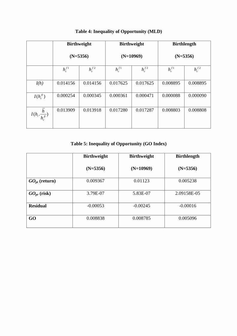
Table 4: Inequality of Opportunity (MLD)

Birthweight

(N=5356)

Birthweight

(N=10969)

Birthlength

(N=5356)

1fch 2f

ch 1fch 2f

ch 1fch 2f

ch

I(h) 0.014156 0.014156 0.017625 0.017625 0.008895 0.008895

)( fichI 0.000254 0.000345 0.000361 0.000471 0.000088 0.000090

).(fi

c

ih

hhI

0.013909 0.013918 0.017280 0.017287 0.008803 0.008808

Table 5: Inequality of Opportunity (GO Index)

Birthweight

(N=5356)

Birthweight

(N=10969)

Birthlength

(N=5356)

GOpt (return) 0.009367 0.01123 0.005238

GOpr (risk) 3.79E-07 5.83E-07 2.09158E-05

Residual -0.00053 -0.00245 -0.00016

GO 0.008838 0.008785 0.005096

Table 6: Inequality of Opportunity - Sensitivity Checks

Birthweight

(N=10969)

3fch

8 types

1fch

16 types

2fch

16 types

3fch

16 types

I(h) 0.017625 0.017625 0.017625 0.017625

)( fichI 0.000743 0.000382 0.000517 0.000980

).(fi

c

ih

hhI

0.017375 0.017260 0.017273 0.017473

Table 7: FGT Low Birthweight – Decomposition by Group

Type FGT Population

Share

Absolute

Contribution

Relative

Contribution

Relative

Risk

1 0.074933 0.048702 0.003649 0.095194 1.954622

2 0.049034 0.079748 0.00391 0.102002 1.279054

3 0.065145 0.06286 0.004095 0.106819 1.699316

4 0.036882 0.241155 0.008894 0.232006 0.962062

5 0.051817 0.025937 0.001344 0.035057 1.351621

6 0.03135 0.182336 0.005716 0.149111 0.817781

7 0.049541 0.018454 0.000914 0.023848 1.292294

8 0.028607 0.339779 0.00972 0.253549 0.746217

Population 0.038336 1 0.038336 1 1

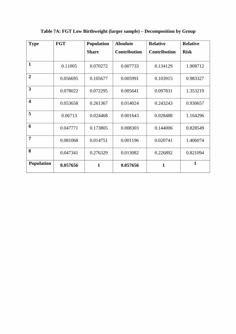
Table 7A: FGT Low Birthweight (larger sample) – Decomposition by Group

Type FGT Population

Share

Absolute

Contribution

Relative

Contribution

Relative

Risk

1 0.11005 0.070272 0.007733 0.134129 1.908712

2 0.056695 0.105677 0.005991 0.103915 0.983327

3 0.078022 0.072295 0.005641 0.097831 1.353219

4 0.053658 0.261367 0.014024 0.243243 0.930657

5 0.06713 0.024468 0.001643 0.028488 1.164296

6 0.047771 0.173805 0.008303 0.144006 0.828549

7 0.081068 0.014751 0.001196 0.020741 1.406074

8 0.047341 0.276329 0.013082 0.226892 0.821094

Population 0.057656 1 0.057656 1 1

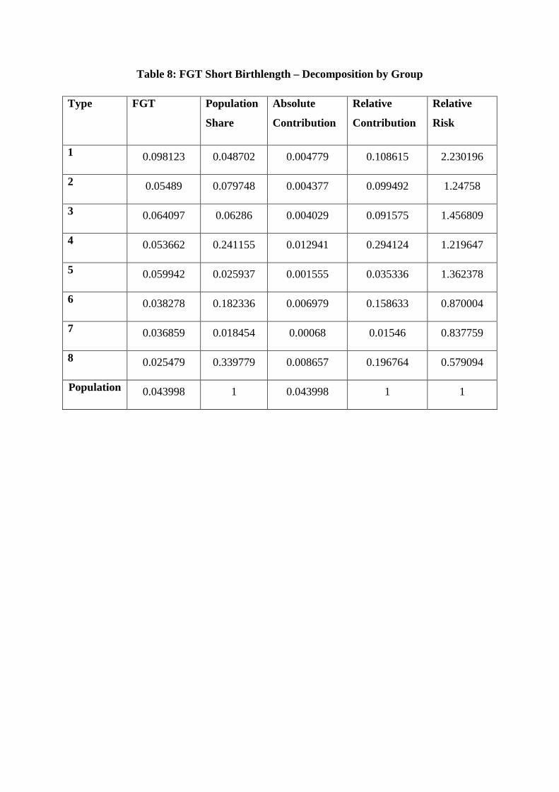
Table 8: FGT Short Birthlength – Decomposition by Group

Type FGT Population

Share

Absolute

Contribution

Relative

Contribution

Relative

Risk

1 0.098123 0.048702 0.004779 0.108615 2.230196

2 0.05489 0.079748 0.004377 0.099492 1.24758

3 0.064097 0.06286 0.004029 0.091575 1.456809

4 0.053662 0.241155 0.012941 0.294124 1.219647

5 0.059942 0.025937 0.001555 0.035336 1.362378

6 0.038278 0.182336 0.006979 0.158633 0.870004

7 0.036859 0.018454 0.00068 0.01546 0.837759

8 0.025479 0.339779 0.008657 0.196764 0.579094

Population 0.043998 1 0.043998 1 1

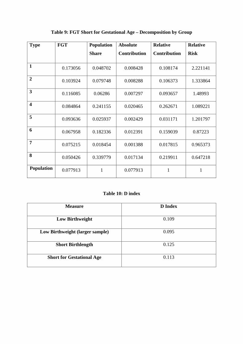
Table 9: FGT Short for Gestational Age – Decomposition by Group

Type FGT Population

Share

Absolute

Contribution

Relative

Contribution

Relative

Risk

1 0.173056 0.048702 0.008428 0.108174 2.221141

2 0.103924 0.079748 0.008288 0.106373 1.333864

3 0.116085 0.06286 0.007297 0.093657 1.48993

4 0.084864 0.241155 0.020465 0.262671 1.089221

5 0.093636 0.025937 0.002429 0.031171 1.201797

6 0.067958 0.182336 0.012391 0.159039 0.87223

7 0.075215 0.018454 0.001388 0.017815 0.965373

8 0.050426 0.339779 0.017134 0.219911 0.647218

Population 0.077913 1 0.077913 1 1

Table 10: D index

Measure D Index

Low Birthweight 0.109

Low Birthweight (larger sample) 0.095

Short Birthlength 0.125

Short for Gestational Age 0.113

References

Almond, D and J. Currie, (2011a) Human Capital Development Before Age Five. Handbookof Labour Economics, 4, 1315-1486.

Almond, D and J. Currie, (2011b) Killing Me Softly: The Fetal Origins Hypothesis. Journalof Economic Perspectives, 25, 153-172.

Araar, A., and JY Duclos (2012) DASP Distributive Analysis Stata Package, UniversiteeLaval, PEP, CIRPEE and World Bank.

Black, S.E., P. Devereux and K. Salvanes (2007). From the Cradle to the Labour Market?The Effect of Birthweight on Adult Outcomes. Quarterly Journal of Economics, 122, 409-439.

Brugha, R., Tully, N., Dicker, P., Shelley, E., Ward, M. and McGee, H. (2009) SLÁN 2007:Survey of Lifestyle, Attitudes and Nutrition in Ireland. Smoking Patterns in Ireland:Implications for policy and services, Department of Health and Children. Dublin: TheStationery Office.

Currie, J., (2011). Inequality at Birth: Some Causes and Consequences. mimeo, PrincetonUniversity.

Cutler, D., Richardson, E., (1997). Measuring the health of the United States population.Brookings papers on Economic activity. Microeconomics 217–271.

Delaney, L., M. McGovern and J. Smith, (2011) From Angela’s Ashes to the Celtic Tiger:Early Life Conditions and Adult Health in Ireland. Journal of Health Economics, 30, 1-10.

Donaldson, D., and J, Weymark. (1980) A Single Parameter Extension of the Gini Indices ofInequality. Journal of Economic Theory, 22, 67-86.

Dworkin, R., (1981) What is Inequality? Part 2: Equality of Resources. Philosophy andPublic Affairs, 10, 283-345.

Figlio, D., J. Guryan, K. Karbownik and J. Roth (2013) The Effects of Poor Neonatal Healthon Children’s Cognitive Development, NBER Working Paper 18846.

Kramer, M.S., L. Seguin, J. Lydon and L. Goulet, (2000) Socio-economic disparities inpregnancy outcome: why do the poor fare so poorly?. Paediatric and Perinatal Epidemiology,14, 194-210.

Madden, D. (2013) The Relationship Between Low Birthweight and Socioeconomic Status inIreland, forthcoming, Journal of Biosocial Science.

McAvoy, H., J. Sturley, S. Burke and K. Balanda. (2006) Unequal at Birth: Inequalities in theOccurrence of Low Birthweight Babies in Ireland. Institute of Public Health in Ireland.

McGovern, M., (2011) Still Unequal at Birth: Socioeconomic Status and Birthweight inIreland. Mimeo.

Niedhammer, I., C. Murrin, D. O’Mahony, S. Daly, J. Morrison and C. Kelleher. (2011)Explanations for Social Inequalities in Preterm Delivery in the Propspective Lifeways Cohortin the Republic of Ireland. European Journal of Public Health, 1-6.

Nybo Andersen A-M and M Osler (2004) Birth Dimensions, Parental Mortality and Mortalityin early Adult Age: a Cohort Study of Danish Men Born in 1953. International Journal ofEpidemiology., 33, 92-99.

Paes de Barros, R., F. Ferreira, J Molinas Vega and J Sanduvi (2009). Measuring Inequalityof Opportunities in Latin America and the Caribbean. World Bank.

Quail, A., J. Williams, C. McCrory, A. Murray and M. Thornton. (2011). A Summary Guideto Wave 1 of the Infant Cohort (at 9 months) of Growing Up in Ireland. Economic andSocial Research Institute, Dublin.

Ramos, X., and D. Van de gaer (2012) Empirical Approaches to Inequality of Opportunity:Principles, Measures and Evidence. IZA Discussion paper 6672.

Risnes, K, L. Vatten, J.Baker et al. (2011) Birthweight and Mortality in Adulthood: ASystematic Review and Meta-Analysis. International Journal of Epidemiology., 40, 647-661.

Rosa Dias, P. and A, Jones (2007) Giving Equality of Opportunity a Fair Innings, HealthEconomics, 16, 109-112.

Romer, J (1998) Equality of Opportunity. Harvard University Press, Harvard.

Romer, J (2002) Equality of Opportunity: A Progress Report. Social Choice and Welfare, 19,455-471.

Saenger, P., P. Czernichow, I. Hughes and P. Reiter (2007) Small for Gestational Age: ShortStature and Beyond, Endocrine Reviews, 28, 219-251.

Salardi, P., 2008. "Brazilian Poverty Between And Within Groups: Decomposition ByGeographical, Group-Specific Poverty Lines," PRUS Working Papers 41, Poverty ResearchUnit at Sussex, University of Sussex.