Borrowing, Depreciation, Taxes in Cash Flow Problems

Scott Matthews12-706 / 19-702

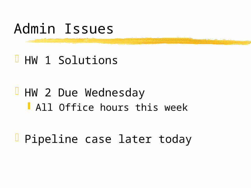
Admin Issues

HW 1 Solutions

HW 2 Due Wednesday All Office hours this week

Pipeline case later today

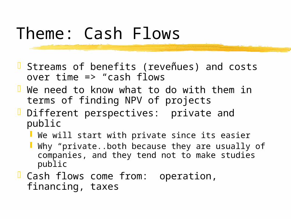
Theme: Cash Flows

Streams of benefits (revenues) and costs over time => “cash flows”

We need to know what to do with them in terms of finding NPV of projects

Different perspectives: private and public We will start with private since its easier Why “private..both because they are usually of

companies, and they tend not to make studies public

Cash flows come from: operation, financing, taxes

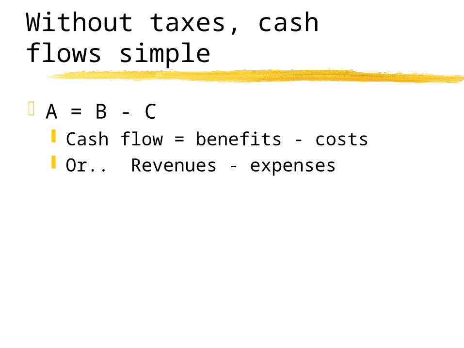
Without taxes, cash flows simple

A = B - C Cash flow = benefits - costs Or.. Revenues - expenses

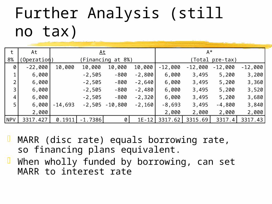
Further Analysis (still no tax)t At

8% (Operation)0 -22,000 10,000 10,000 10,000 10,000 -12,000 -12,000 -12,000 -12,0001 6,000 -2,505 -800 -2,800 6,000 3,495 5,200 3,2002 6,000 -2,505 -800 -2,640 6,000 3,495 5,200 3,3603 6,000 -2,505 -800 -2,480 6,000 3,495 5,200 3,5204 6,000 -2,505 -800 -2,320 6,000 3,495 5,200 3,6805 6,000 -14,693 -2,505 -10,800 -2,160 -8,693 3,495 -4,800 3,840

2,000 2,000 2,000 2,000 2,000NPV 3317.427 0.1911 -1.7386 0 1E-12 3317.62 3315.69 3317.4 3317.43

At(Financing at 8%)

A*(Total pre-tax)

MARR (disc rate) equals borrowing rate, so financing plans equivalent.

When wholly funded by borrowing, can set MARR to interest rate

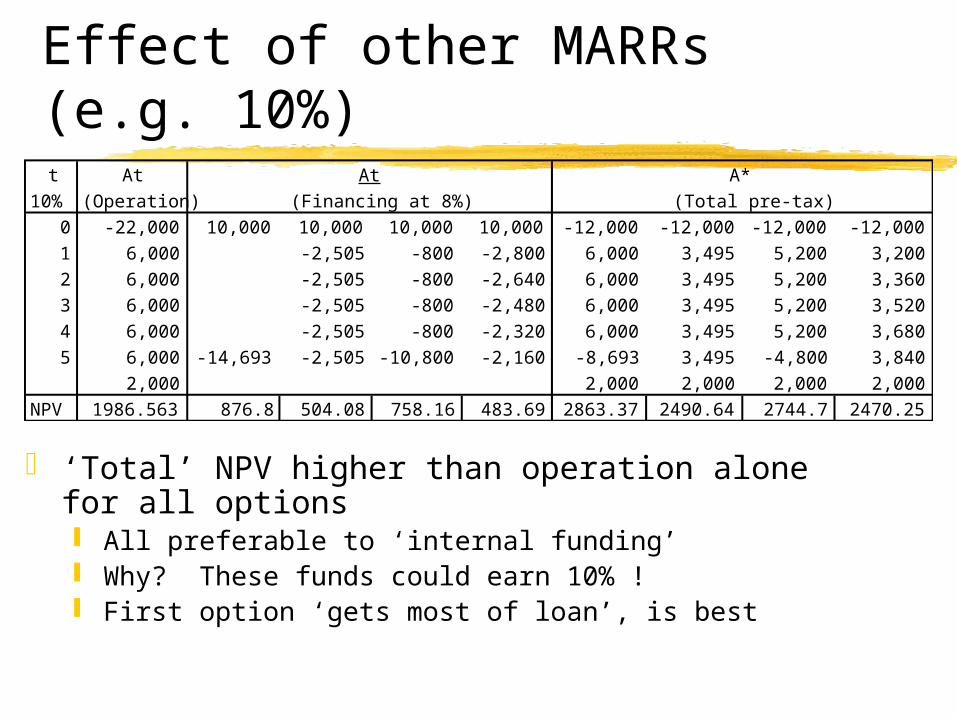
Effect of other MARRs (e.g. 10%)t At

10% (Operation)0 -22,000 10,000 10,000 10,000 10,000 -12,000 -12,000 -12,000 -12,0001 6,000 -2,505 -800 -2,800 6,000 3,495 5,200 3,2002 6,000 -2,505 -800 -2,640 6,000 3,495 5,200 3,3603 6,000 -2,505 -800 -2,480 6,000 3,495 5,200 3,5204 6,000 -2,505 -800 -2,320 6,000 3,495 5,200 3,6805 6,000 -14,693 -2,505 -10,800 -2,160 -8,693 3,495 -4,800 3,840

2,000 2,000 2,000 2,000 2,000NPV 1986.563 876.8 504.08 758.16 483.69 2863.37 2490.64 2744.7 2470.25

At A*(Financing at 8%) (Total pre-tax)

‘Total’ NPV higher than operation alone for all options All preferable to ‘internal funding’ Why? These funds could earn 10% ! First option ‘gets most of loan’, is best

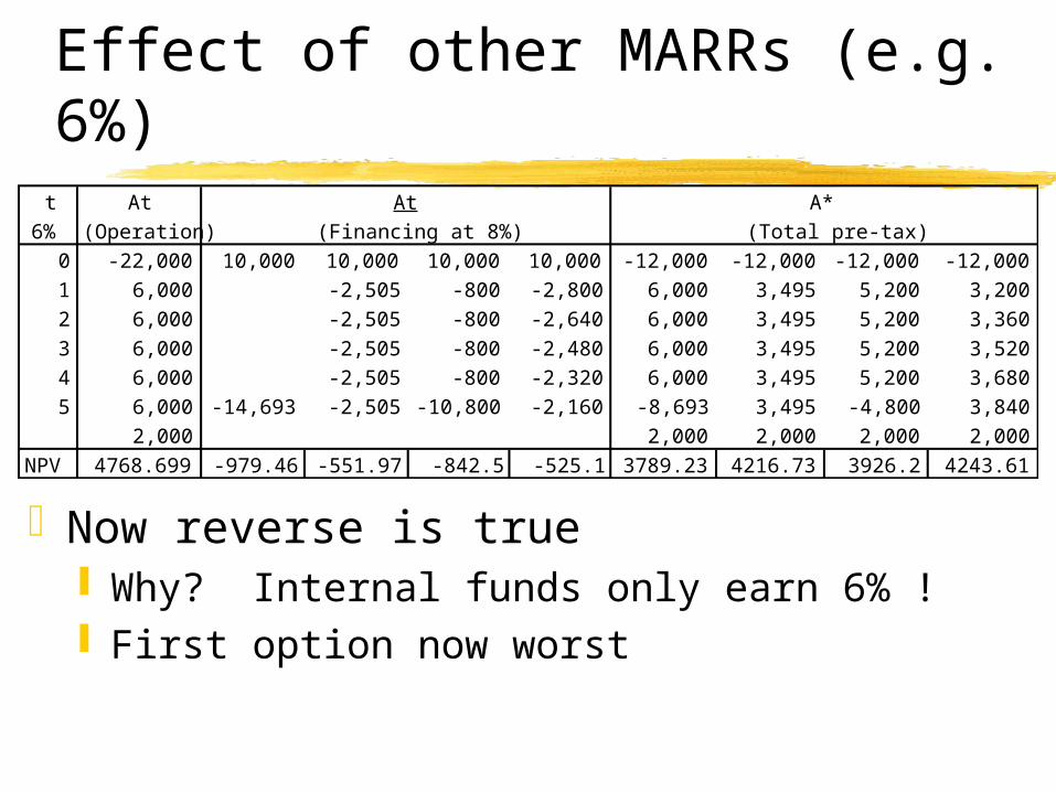
Effect of other MARRs (e.g. 6%)t At

6% (Operation)0 -22,000 10,000 10,000 10,000 10,000 -12,000 -12,000 -12,000 -12,0001 6,000 -2,505 -800 -2,800 6,000 3,495 5,200 3,2002 6,000 -2,505 -800 -2,640 6,000 3,495 5,200 3,3603 6,000 -2,505 -800 -2,480 6,000 3,495 5,200 3,5204 6,000 -2,505 -800 -2,320 6,000 3,495 5,200 3,6805 6,000 -14,693 -2,505 -10,800 -2,160 -8,693 3,495 -4,800 3,840

2,000 2,000 2,000 2,000 2,000NPV 4768.699 -979.46 -551.97 -842.5 -525.1 3789.23 4216.73 3926.2 4243.61

At A*(Financing at 8%) (Total pre-tax)

Now reverse is true Why? Internal funds only earn 6% ! First option now worst

Bonds

Done similar to loans, but mechanically different

Usually pay annual interest only, then repay interest and entire principal in yr. n Similar to financing option #3 in previous

slides There are other, less common bond

methods

Tax Effects of Financing

Companies deduct interest expense Bt=total pre-tax operating benefits

Excluding loan receipts

Ct=total operating pre-tax expenses Excluding loan payments

At= Bt- Ct = net pre-tax operating cash flow A,B,C: financing cash flows A*,B*,C*: pre-tax totals / all sources

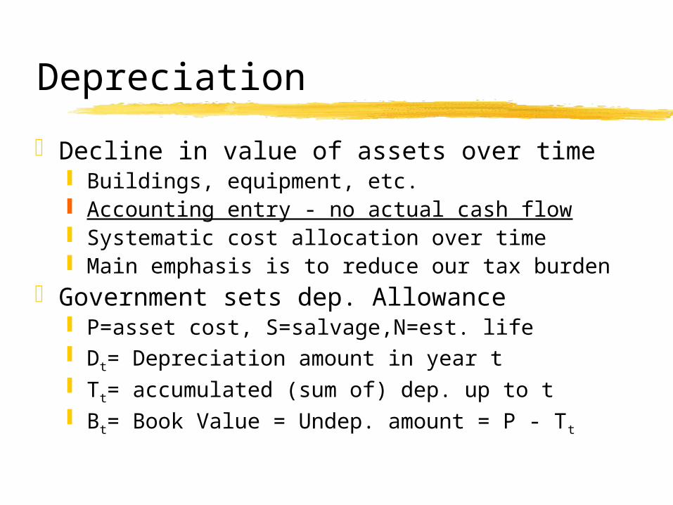
Depreciation

Decline in value of assets over time Buildings, equipment, etc. Accounting entry - no actual cash flow Systematic cost allocation over time Main emphasis is to reduce our tax burden

Government sets dep. Allowance P=asset cost, S=salvage,N=est. life Dt= Depreciation amount in year t Tt= accumulated (sum of) dep. up to t Bt= Book Value = Undep. amount = P - Tt

After-tax cash flows

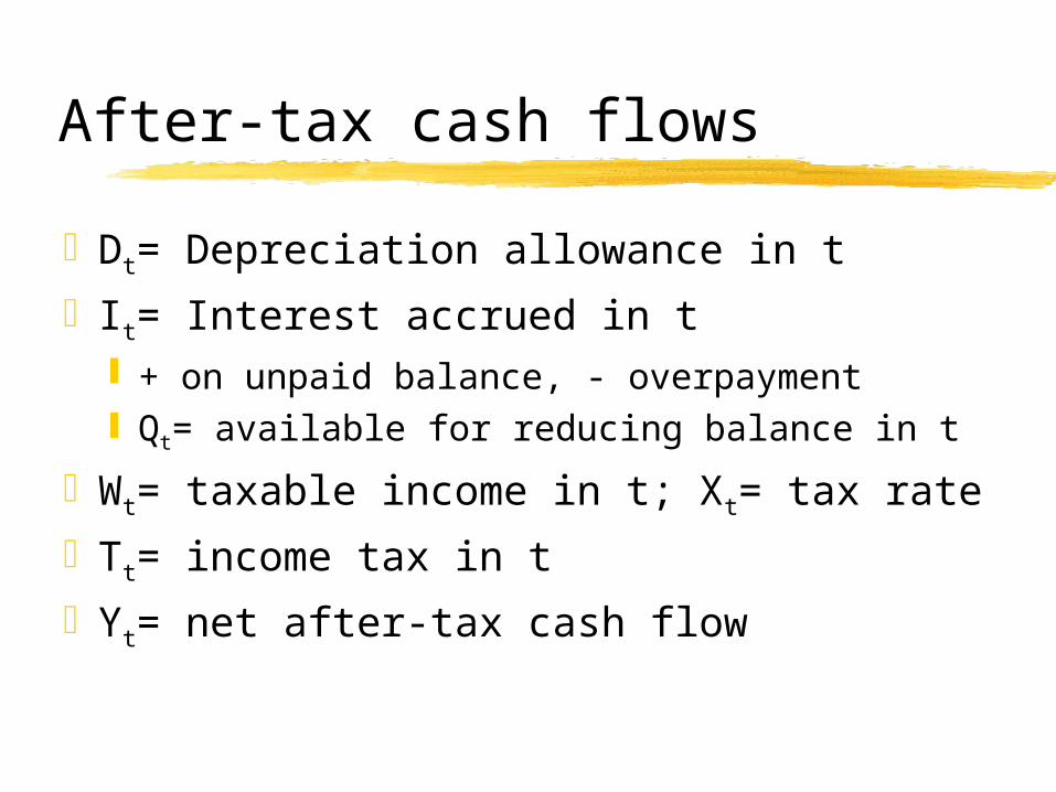
Dt= Depreciation allowance in t

It= Interest accrued in t + on unpaid balance, - overpayment Qt= available for reducing balance in t

Wt= taxable income in t; Xt= tax rate

Tt= income tax in t

Yt= net after-tax cash flow

Equations

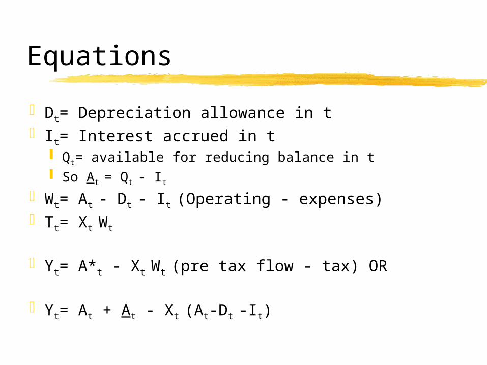
Dt= Depreciation allowance in tIt= Interest accrued in t

Qt= available for reducing balance in t So At = Qt - It

Wt= At - Dt - It (Operating - expenses)Tt= Xt Wt

Yt= A*t - Xt Wt (pre tax flow - tax) OR

Yt= At + At - Xt (At-Dt -It)

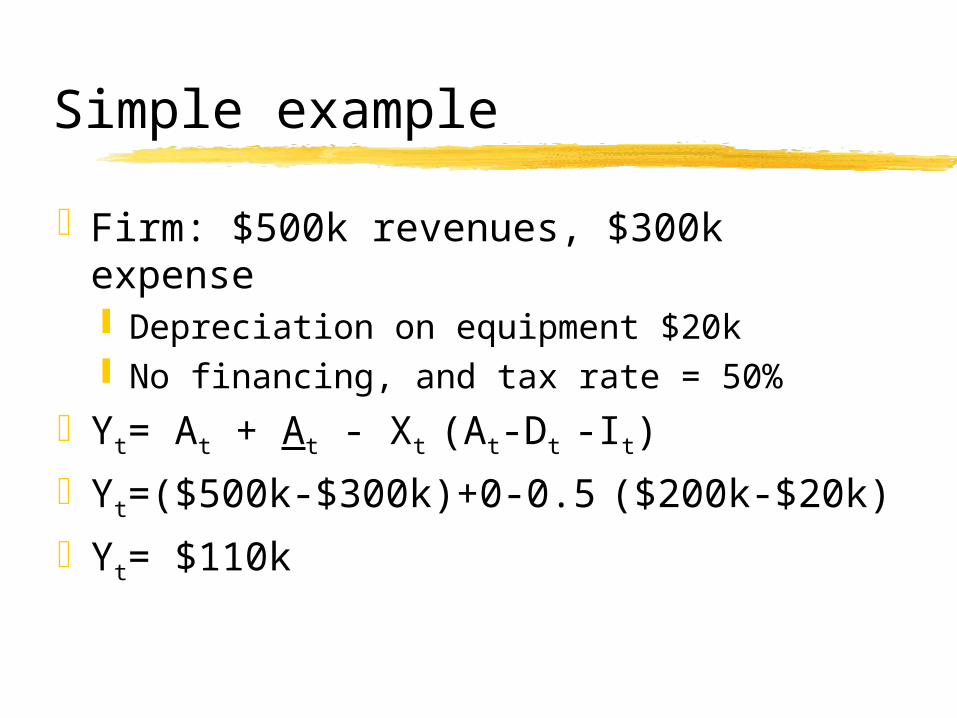
Simple example

Firm: $500k revenues, $300k expense Depreciation on equipment $20k No financing, and tax rate = 50%

Yt= At + At - Xt (At-Dt -It)

Yt=($500k-$300k)+0-0.5 ($200k-$20k)

Yt= $110k

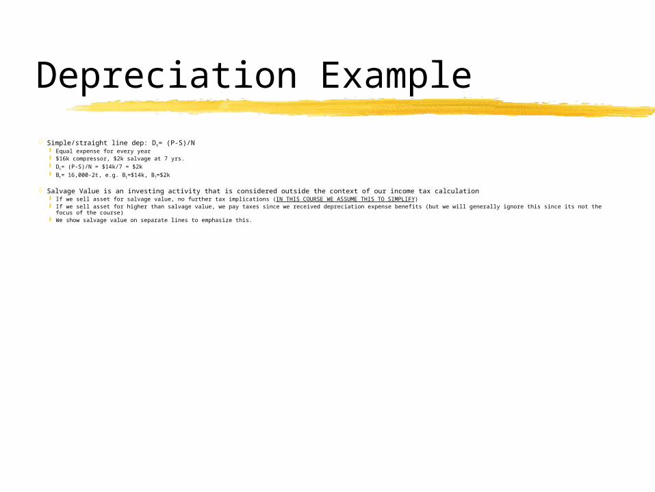
Depreciation Example

Simple/straight line dep: Dt= (P-S)/N Equal expense for every year $16k compressor, $2k salvage at 7 yrs. Dt= (P-S)/N = $14k/7 = $2k Bt= 16,000-2t, e.g. B1=$14k, B7=$2k

Salvage Value is an investing activity that is considered outside the context of our income tax calculation If we sell asset for salvage value, no further tax implications (IN THIS COURSE WE ASSUME THIS TO SIMPLIFY) If we sell asset for higher than salvage value, we pay taxes since we received depreciation expense benefits (but we will generally ignore this since its not the focus of the course) We show salvage value on separate lines to emphasize this.

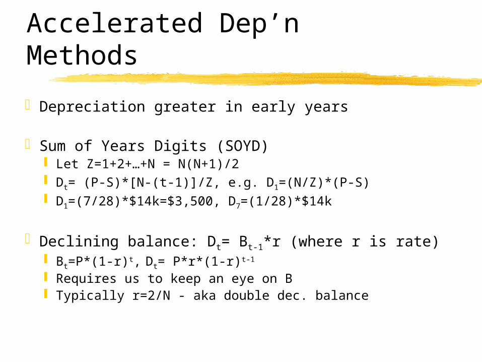
Accelerated Dep’n Methods

Depreciation greater in early years

Sum of Years Digits (SOYD) Let Z=1+2+…+N = N(N+1)/2 Dt= (P-S)*[N-(t-1)]/Z, e.g. D1=(N/Z)*(P-S) D1=(7/28)*$14k=$3,500, D7=(1/28)*$14k

Declining balance: Dt= Bt-1*r (where r is rate) Bt=P*(1-r)t, Dt= P*r*(1-r)t-1

Requires us to keep an eye on B Typically r=2/N - aka double dec. balance

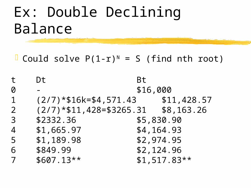
Ex: Double Declining Balance

Could solve P(1-r)N = S (find nth root)

t Dt Bt0 - $16,0001 (2/7)*$16k=$4,571.43 $11,428.572 (2/7)*$11,428=$3265.31 $8,163.263 $2332.36 $5,830.904 $1,665.97 $4,164.935 $1,189.98 $2,974.956 $849.99 $2,124.967 $607.13** $1,517.83**

Notes on Example

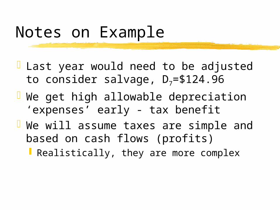
Last year would need to be adjusted to consider salvage, D7=$124.96

We get high allowable depreciation ‘expenses’ early - tax benefit

We will assume taxes are simple and based on cash flows (profits) Realistically, they are more complex

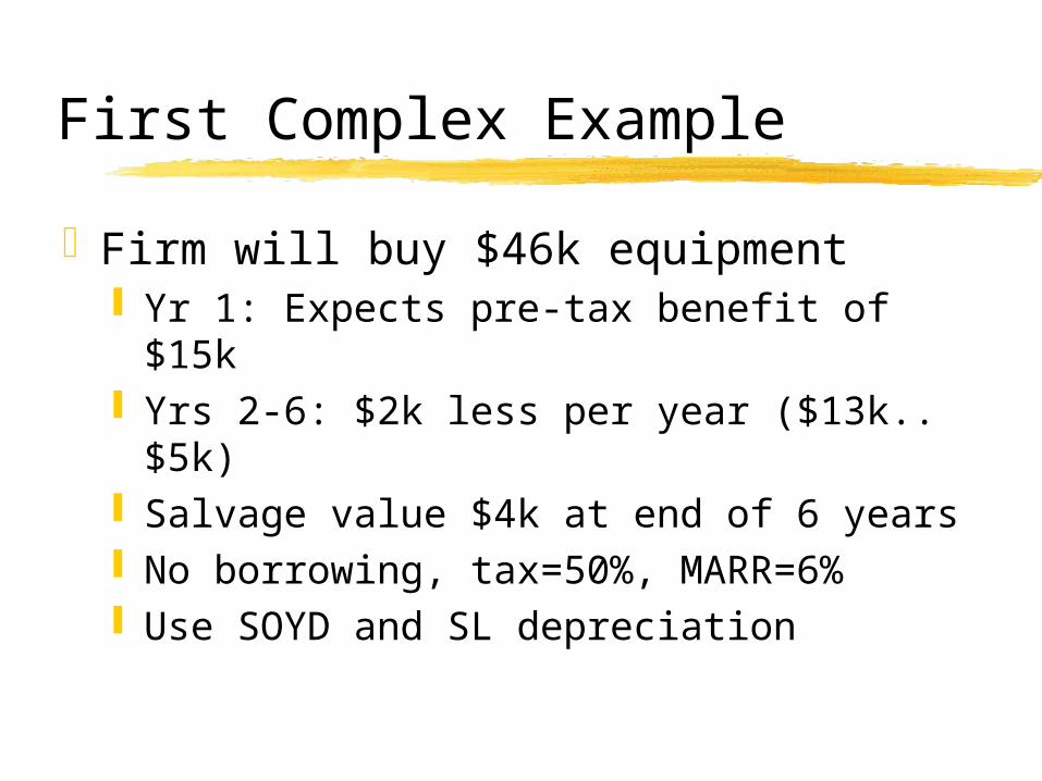
First Complex Example

Firm will buy $46k equipment Yr 1: Expects pre-tax benefit of $15k Yrs 2-6: $2k less per year ($13k..$5k) Salvage value $4k at end of 6 years No borrowing, tax=50%, MARR=6% Use SOYD and SL depreciation

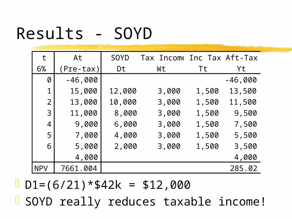
Results - SOYD

D1=(6/21)*$42k = $12,000SOYD really reduces taxable income!

t At SOYD Tax Income Inc Tax Aft-Tax6% (Pre-tax) Dt Wt Tt Yt

0 -46,000 -46,0001 15,000 12,000 3,000 1,500 13,5002 13,000 10,000 3,000 1,500 11,5003 11,000 8,000 3,000 1,500 9,5004 9,000 6,000 3,000 1,500 7,5005 7,000 4,000 3,000 1,500 5,5006 5,000 2,000 3,000 1,500 3,500

4,000 4,000NPV 7661.004 285.02

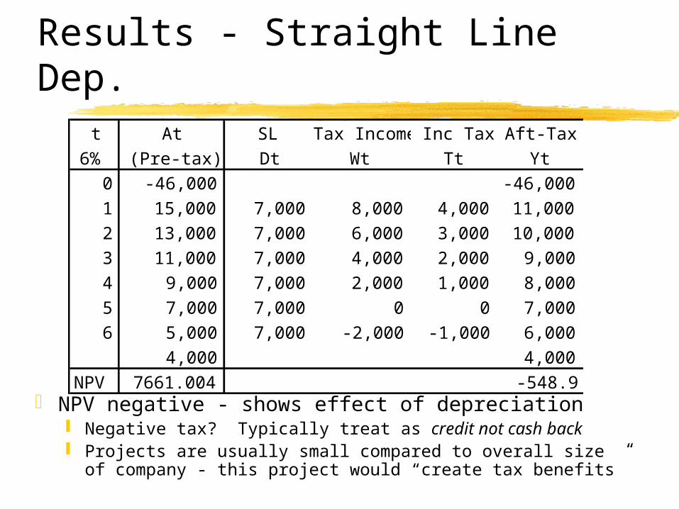
Results - Straight Line Dep.

NPV negative - shows effect of depreciation Negative tax? Typically treat as credit not cash back Projects are usually small compared to overall size of

company - this project would “create tax benefits”

t At SL Tax Income Inc Tax Aft-Tax6% (Pre-tax) Dt Wt Tt Yt

0 -46,000 -46,0001 15,000 7,000 8,000 4,000 11,0002 13,000 7,000 6,000 3,000 10,0003 11,000 7,000 4,000 2,000 9,0004 9,000 7,000 2,000 1,000 8,0005 7,000 7,000 0 0 7,0006 5,000 7,000 -2,000 -1,000 6,000

4,000 4,000NPV 7661.004 -548.9

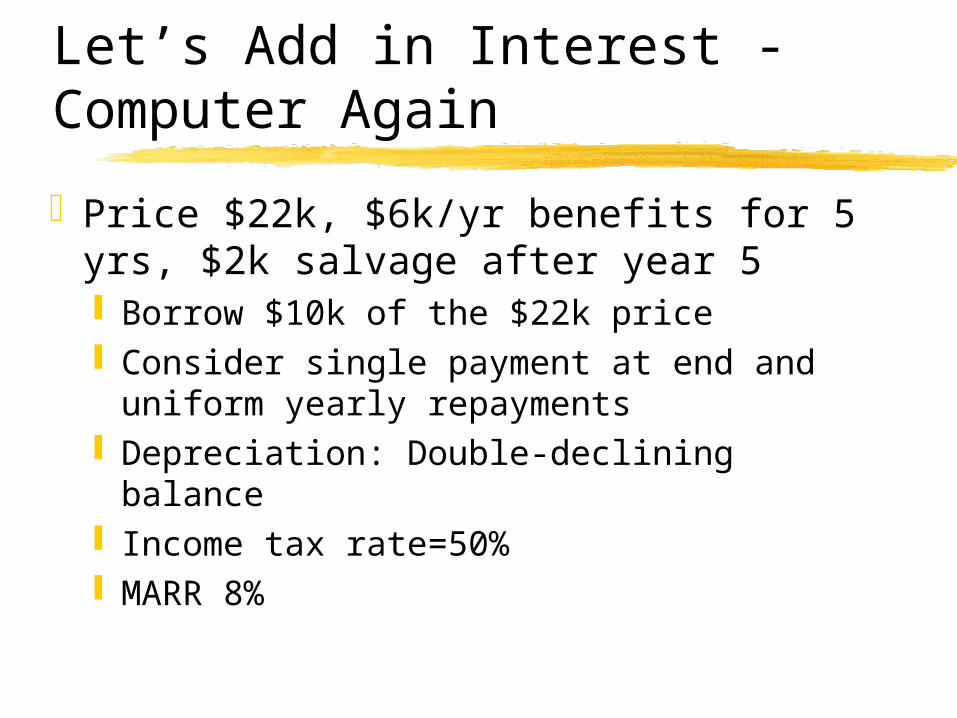
Let’s Add in Interest - Computer Again

Price $22k, $6k/yr benefits for 5 yrs, $2k salvage after year 5 Borrow $10k of the $22k price Consider single payment at end and

uniform yearly repayments Depreciation: Double-declining balance Income tax rate=50% MARR 8%

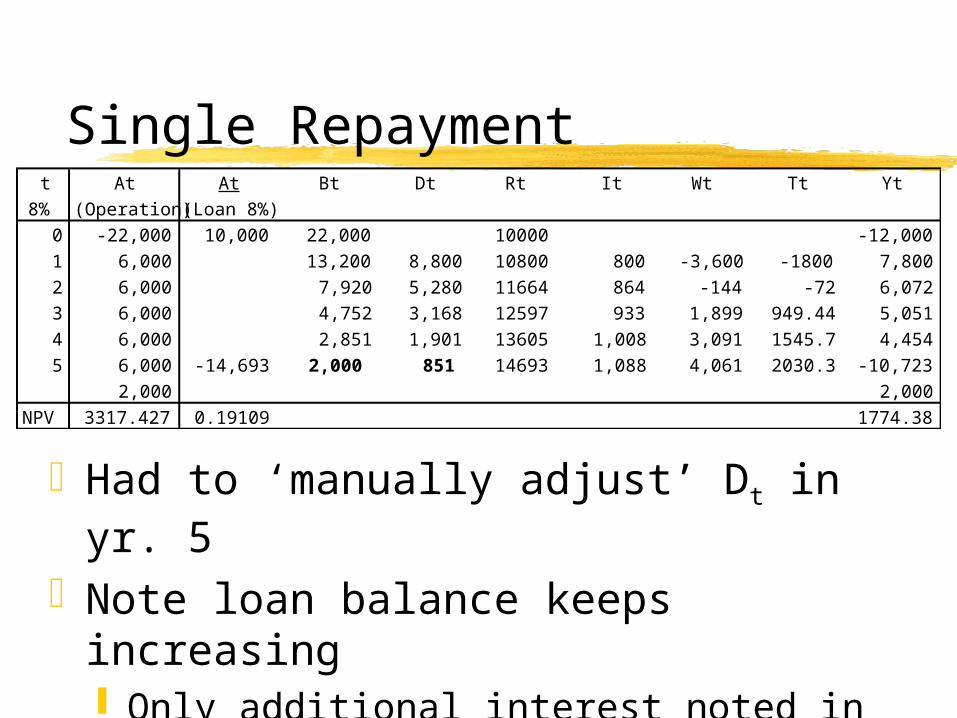
t At At Bt Dt Rt It Wt Tt Yt8% (Operation) (Loan 8%)

0 -22,000 10,000 22,000 10000 -12,0001 6,000 13,200 8,800 10800 800 -3,600 -1800 7,8002 6,000 7,920 5,280 11664 864 -144 -72 6,0723 6,000 4,752 3,168 12597 933 1,899 949.44 5,0514 6,000 2,851 1,901 13605 1,008 3,091 1545.7 4,4545 6,000 -14,693 2,000 851 14693 1,088 4,061 2030.3 -10,723

2,000 2,000NPV 3317.427 0.19109 1774.38

Single Repayment

Had to ‘manually adjust’ Dt in yr. 5Note loan balance keeps increasing

Only additional interest noted in It as interest expense

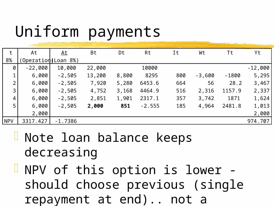
Uniform paymentst At At Bt Dt Rt It Wt Tt Yt

8% (Operation) (Loan 8%)0 -22,000 10,000 22,000 10000 -12,0001 6,000 -2,505 13,200 8,800 8295 800 -3,600 -1800 5,2952 6,000 -2,505 7,920 5,280 6453.6 664 56 28.2 3,4673 6,000 -2,505 4,752 3,168 4464.9 516 2,316 1157.9 2,3374 6,000 -2,505 2,851 1,901 2317.1 357 3,742 1871 1,6245 6,000 -2,505 2,000 851 -2.555 185 4,964 2481.8 1,013

2,000 2,000NPV 3317.427 -1.7386 974.707

Note loan balance keeps decreasingNPV of this option is lower - should

choose previous (single repayment at end).. not a general result

Leasing

‘Make payments to owner’ instead of actually purchasing the asset Since you do not own it, you can not

take depreciation expense Lease payments are just a standard

expense (i.e., part of the Ct stream) At= Bt - Ct ; Yt= At - At Xt

Tradeoff is lower expenses vs. loss of depreciation/interest tax benefits

Show of Hands Example

Choice #1: $50 today or $100 paid 1 year from now? Why?

Choice #2: $50 to be paid in 5 years or $100 in 6

years? Why?

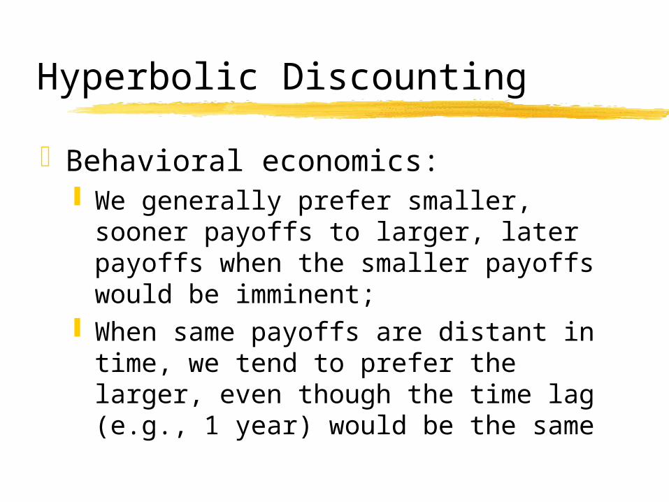
Hyperbolic Discounting

Behavioral economics: We generally prefer smaller, sooner payoffs

to larger, later payoffs when the smaller payoffs would be imminent;

When same payoffs are distant in time, we tend to prefer the larger, even though the time lag (e.g., 1 year) would be the same

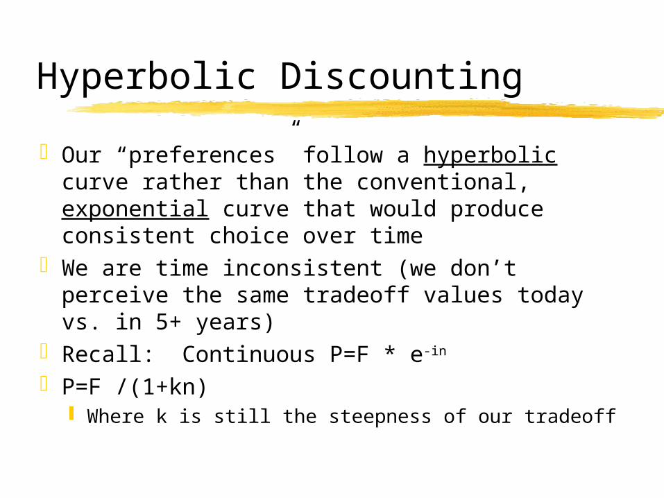
Hyperbolic Discounting

Our “preferences” follow a hyperbolic curve rather than the conventional, exponential curve that would produce consistent choice over time

We are time inconsistent (we don’t perceive the same tradeoff values today vs. in 5+ years)

Recall: Continuous P=F * e-in

P=F /(1+kn) Where k is still the steepness of our tradeoff

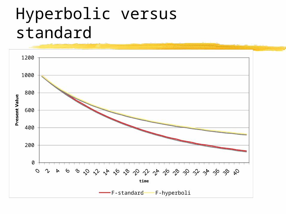
Hyperbolic versus standard

0

200

400

600

800

1000

1200

0 2 4 6 8 10 12 14 16 18 20 22 24 26 28 30 32 34 36 38 40time

Present Value

F-standard F-hyperbolic

Hyperbolic Discounting-Implications

If we actually have hyperbolic preferences

What do our discount rates look like?

How would that affect our preferences for social projects, especially those with long time horizons? Time inconsistency known in advance

Pipeline Case

Hand them InDiscussion / OverviewModels BuiltSample Model

What is Missing in these models?Did they build it?