Embed Size (px)
Citation preview
BOSTON UNIVERSITY
COLLEGE OF ENGINEERING
Dissertation
NEURAL NETWORK COMPUTING USING ON-CHIP
ACCELERATORS
by
SCHUYLER ELDRIDGE
B.S., Boston University, 2010
Submitted in partial fulfillment of the
requirements for the degree of
Doctor of Philosophy
2016

© 2016 bySCHUYLER ELDRIDGEAll rights reserved
Approved by
First Reader
Ajay J. Joshi, PhDAssociate Professor of Electrical and Computer Engineering
Second Reader
Allyn E. Hubbard, PhDProfessor of Biomedical EngineeringProfessor of Electrical and Computer Engineering
Third Reader
Martin C. Herbordt, PhDProfessor of Electrical and Computer Engineering
Fourth Reader
Jonathan Appavoo, PhDAssociate Professor of Computer Science

. . . he looked carefully at the barman.
“A dry martini,” he said. “One. In a deep champagne goblet.”
“Oui, monsieur.”
“Just a moment. Three measures of Gordon’s, one of vodka, half a mea-sure of Kina Lillet. Shake it very well until it’s ice-cold, then add a largethin slice of lemon peel. Got it?”
“Certainly, monsieur.” The barman seemed pleased with the idea.
“Gosh, that’s certainly a drink,” said Leiter.
Bond laughed. “When I’m . . . er . . . concentrating,” he explained, “I neverhave more than one drink before dinner. But I do like that one to be largeand very strong and very cold and very well-made. I hate small portionsof anything, particularly when they taste bad. This drink’s my own inven-tion. I’m going to patent it when I can think of a good name.”
[Fleming, 1953]
iv
Acknowledgments
All of this work was enabled by my gracious funding sources over the past six years.
In my first year, Prof. Ayse Coskun helped me secure a Dean’s Fellowship through
Boston University. My second year was funded through Boston University’s former
Center of Excellence for Learning in Education, Science, and Technology (CELEST)
working with Dr. Florian Raudies and Dr. Max Versace. Florian and Max were
instrumental in providing my first introduction to biological modeling and neural
networks.
I am incredibly thankful for funding through the subsequent four years from the
National Aeronautics and Space Administration (NASA) via a Space Technology
Research Fellowship (NSTRF). This provided me with the unbelievable opportunity
to work at NASA Jet Propulsion Lab (JPL) for three summers with Dr. Adrian
Stoica. Adrian’s discussions were invaluable and I’m incredibly thankful for him
acting as host, mentor, instigator, and friend.
Digressing, I must mention a number of people who guided me along the way up
to this point and on whose wisdom I drew during this process. Luis Lovett, my figure
skating coach in Virginia, taught me that there’s beauty just in the effort of trying.
Allen Schramm, my choreographer, similarly showed me the brilliance of abandoning
perfection for artistic immersion within and without. Tommy Litz, my technical
coach, impressed on me that eventually you’ll hit a point and you just have to be a
man. And finally, Slavka Kohout, my competitive coach, taught me the unforgettable
lesson that the crowd really does just want to see blood.1
1c.f. [Hemingway, 1926]:
Romero’s bull-fighting gave real emotion, because he kept the absolute purity of linein his movements and always quietly and calmly let the horns pass him close eachtime. He did not have to emphasize their closeness. Brett saw how something thatwas beautiful done close to the bull was ridiculous if it were done a little way off. Itold her how since the death of Joselito all the bull-fighters had been developing atechnique that simulated this appearance of danger in order to give a fake emotional
v

Naturally, I’m thankful for the help and guidance of my advisor, Prof. Ajay Joshi,
who helped me through (and stuck with me) during the meandering, confusing, and
dead-end-riddled path that I took. I am also forever indebted to Prof. Jonathan
Appavoo, acting as an unofficial advisor, collaborator, and friend over the past three
years. My one regret throughout this whole process was not getting to know him
sooner.
It goes without saying that none of this would have been possible without the
friendship of my parents, John and Diana Eldridge. They have consistently been my
wellspring of support throughout my life. This is further remarkable considering our
atypical family and all of the extraneous and incredibly challenging circumstances
we’ve collectively experienced. Furthermore, my lifelong friends Alex Scott and Peter
Achenbaum have always been there and, critically, always ready for a cocktail.
Finally, as I’ve attempted to impress on new PhD students, a PhD is a psycholog-
ical gauntlet testing your mental limits. It’s hard, it’s terrible, and it will push you
in every way imaginable, but it’s one of the only times in your lives when you can
lose yourself in maniacal focus. It’s a lot like wandering into a forest.2 It’s pretty for
a while, but you will eventually, without fail, become (seemingly) irrevocably lost.
Be worried, but not overly so—there’s a catharsis coming. You will hit a point and
you’ll take ownership,3 and after that your perspective in all things changes. So, it
does get better, I promise, and there’s beauty in all of it.
feeling, while the bull-fighter was really safe. Romero had the old thing, the holdingof his purity of line through the maximum of exposure, while he dominated the bullby making him realize he was unattainable, while he prepared him for the killing.
2c.f. [The Cure, 1980]3c.f. [The Cure, 1985]
vi
NEURAL NETWORK COMPUTING USING ON-CHIP
ACCELERATORS
SCHUYLER ELDRIDGE
Boston University, College of Engineering, 2016
Major Professor: Ajay J. Joshi, PhDAssociate Professor of Electrical and ComputerEngineering
ABSTRACT
The use of neural networks, machine learning, or artificial intelligence, in its broadest
and most controversial sense, has been a tumultuous journey involving three distinct
hype cycles and a history dating back to the 1960s. Resurgent, enthusiastic interest
in machine learning and its applications bolsters the case for machine learning as a
fundamental computational kernel. Furthermore, researchers have demonstrated that
machine learning can be utilized as an auxiliary component of applications to enhance
or enable new types of computation such as approximate computing or automatic par-
allelization. In our view, machine learning becomes not the underlying application,
but a ubiquitous component of applications. This view necessitates a different ap-
proach towards the deployment of machine learning computation that spans not only
hardware design of accelerator architectures, but also user and supervisor software to
enable the safe, simultaneous use of machine learning accelerator resources.
In this dissertation, we propose a multi-transaction model of neural network com-
putation to meet the needs of future machine learning applications. We demonstrate
that this model, encompassing a decoupled backend accelerator for inference and
vii
learning from hardware and software for managing neural network transactions can
be achieved with low overhead and integrated with a modern RISC-V microprocessor.
Our extensions span user and supervisor software and data structures and, coupled
with our hardware, enable multiple transactions from different address spaces to ex-
ecute simultaneously, yet safely. Together, our system demonstrates the utility of
a multi-transaction model to increase energy efficiency improvements and improve
overall accelerator throughput for machine learning applications.
viii
Preface
Neural Networks, machine learning, and artificial intelligence—some of the most
hyped technologies of the past half century—have seen a dramatic, recent resurgence
towards solving many hard yet computable problems. However, it is with the utmost
caution that the reader must temper their enthusiasm, as I have been forced to over
the duration of the following work. Nevertheless, neural networks are a very powerful
tool, while not truly biological to a purist, that reflect some of the structure of the
brain. These biological machines, evolved over millennia, must indicate a viable
computational substrate for processing the world around us. It is my belief, a belief
shared by others, that this style of computation provides a way forward—beyond the
current difficulties of semiconductor technology—towards more efficient, biologically-
inspired systems capable of providing the next great leap for computation. What
follows, broadly, concerns the design, analysis, and evaluation of hybrid systems that
bring neural networks as close as possible to traditional computer architectures. While
I admit that such architectures are only a stopgap, I hope that this will contribute
towards that aforementioned way forward.
ix
Contents
1 Introduction 1
1.1 Background . . . . . . . . . . . . . . . . . . . . . . . . . . . . . . . . 1
1.1.1 An ontology for computation . . . . . . . . . . . . . . . . . . 4
1.1.2 Machine learning accelerators of the future . . . . . . . . . . . 6
1.2 Motivating Applications . . . . . . . . . . . . . . . . . . . . . . . . . 7
1.3 Outline of Contributions . . . . . . . . . . . . . . . . . . . . . . . . . 9
1.3.1 Thesis statement . . . . . . . . . . . . . . . . . . . . . . . . . 9
1.3.2 Contributions . . . . . . . . . . . . . . . . . . . . . . . . . . . 10
1.4 Dissertation Outline . . . . . . . . . . . . . . . . . . . . . . . . . . . 12
2 Background 14
2.1 A Brief History of Neural Networks . . . . . . . . . . . . . . . . . . . 14
2.1.1 Neural networks and early computer science . . . . . . . . . . 14
2.1.2 Criticisms of neural networks and artificial intelligence . . . . 18
2.1.3 Modern resurgence as machine learning . . . . . . . . . . . . . 21
2.2 Neural Network Software and Hardware . . . . . . . . . . . . . . . . 23
2.2.1 Software . . . . . . . . . . . . . . . . . . . . . . . . . . . . . . 24
2.2.2 Hardware . . . . . . . . . . . . . . . . . . . . . . . . . . . . . 25
2.2.3 Context of this dissertation . . . . . . . . . . . . . . . . . . . 28
3 T-fnApprox: Hardware Support for Fine-Grained Function Approx-
imation using MLPs 31
3.1 Function Approximation . . . . . . . . . . . . . . . . . . . . . . . . . 32
x
3.1.1 CORDIC and Unified CORDIC . . . . . . . . . . . . . . . . . 34
3.2 A Fixed-topology Neural Network Accelerator . . . . . . . . . . . . . 36
3.2.1 Approximation capability . . . . . . . . . . . . . . . . . . . . 39
3.3 Evaluation . . . . . . . . . . . . . . . . . . . . . . . . . . . . . . . . . 42
3.3.1 Energy efficiency . . . . . . . . . . . . . . . . . . . . . . . . . 42
3.3.2 Comparison against traditional floating point . . . . . . . . . 43
3.3.3 Affect on application benchmarks . . . . . . . . . . . . . . . . 47
3.4 Approximation and Fixed-topology Neural Network Accelerators . . . 48
4 X-FILES: Software/Hardware for Neural Networks as First Class
Primitives 52
4.1 Motivation: Neural Networks as Function Primitives . . . . . . . . . 52
4.2 X-FILES: Software and Hardware for Transaction Management . . . 57
4.2.1 X-FILES Hardware Arbiter . . . . . . . . . . . . . . . . . . . 60
4.2.2 Supervisor data structures: the ASID–NNID Table . . . . . . . 63
4.2.3 Supervisor and user API . . . . . . . . . . . . . . . . . . . . . 67
4.3 Operating System Integration . . . . . . . . . . . . . . . . . . . . . . 69
4.3.1 RISC-V Proxy Kernel . . . . . . . . . . . . . . . . . . . . . . 69
4.3.2 RISCV-V Linux port . . . . . . . . . . . . . . . . . . . . . . . 70
4.4 Summary . . . . . . . . . . . . . . . . . . . . . . . . . . . . . . . . . 72
5 DANA: An X-FILES Accelerator for Neural Network Computation 73
5.1 Motivation and Guidelines for a General Neural Network Accelerator 74
5.2 DANA: A Dynamically Allocated Neural Network Accelerator . . . . 77
5.2.1 Transaction Table . . . . . . . . . . . . . . . . . . . . . . . . . 78
5.2.2 Configuration Cache . . . . . . . . . . . . . . . . . . . . . . . 79
5.2.3 ASID–NNID Table Walker . . . . . . . . . . . . . . . . . . . . . 82
5.2.4 Control module . . . . . . . . . . . . . . . . . . . . . . . . . . 83
xi
5.2.5 Processing Elements . . . . . . . . . . . . . . . . . . . . . . . 84
5.2.6 Scratchpad memories . . . . . . . . . . . . . . . . . . . . . . . 86
5.3 Operation for Neural Network Transactions . . . . . . . . . . . . . . 88
5.3.1 Feedforward computation . . . . . . . . . . . . . . . . . . . . 88
5.3.2 Learning . . . . . . . . . . . . . . . . . . . . . . . . . . . . . . 89
5.4 Summary . . . . . . . . . . . . . . . . . . . . . . . . . . . . . . . . . 91
6 Evaluation of X-FILES/DANA 92
6.1 Different Implementations of X-FILES/DANA . . . . . . . . . . . . . 92
6.2 X-FILES/DANA in SystemVerilog . . . . . . . . . . . . . . . . . . . 95
6.2.1 Power and latency . . . . . . . . . . . . . . . . . . . . . . . . 96
6.2.2 Single and multi-transaction throughput . . . . . . . . . . . . 101
6.3 Rocket + X-FILES/DANA . . . . . . . . . . . . . . . . . . . . . . . . 107
6.4 Summary . . . . . . . . . . . . . . . . . . . . . . . . . . . . . . . . . 110
7 Conclusion 111
7.1 Summary of Contributions . . . . . . . . . . . . . . . . . . . . . . . . 111
7.2 Limitations of X-FILES/DANA . . . . . . . . . . . . . . . . . . . . . 112
7.3 Future Work . . . . . . . . . . . . . . . . . . . . . . . . . . . . . . . . 114
7.3.1 Transaction granularity . . . . . . . . . . . . . . . . . . . . . . 114
7.3.2 Variable transaction priority . . . . . . . . . . . . . . . . . . . 115
7.3.3 Asynchronous in-memory input–output queues . . . . . . . . . 116
7.3.4 New X-FILES backends . . . . . . . . . . . . . . . . . . . . . 117
7.3.5 Linux kernel modifications . . . . . . . . . . . . . . . . . . . . 118
7.4 Final Remarks . . . . . . . . . . . . . . . . . . . . . . . . . . . . . . . 118
References 119
Curriculum Vitae 129
xii
List of Tables
2.1 Related work on neural network software and hardware . . . . . . . . 23
3.1 Identities from Unified CORDIC . . . . . . . . . . . . . . . . . . . . . 35
3.2 Scaling steps for Unified CORDIC . . . . . . . . . . . . . . . . . . . . 36
3.3 Error for neural networks approximating transcendental functions . . 40
3.4 Accelerator configurations with minimum energy delay error product 43
3.5 Error and energy of T-fnApprox approximating transcendental functions 43
3.6 Area, frequency, and energy of floating point transcendental functions 45
3.7 Energy delay product of T-fnApprox applied to transcendental functions 46
3.8 Percentage of execution time for transcendental functions in PARSEC 48
3.9 Error of PARSEC applications with T-fnApprox . . . . . . . . . . . 49
4.1 X-FILES Hardware Arbiter Transaction Table bit fields . . . . . . . . 61
4.2 Exceptions generated by X-FILES/DANA . . . . . . . . . . . . . . . 66
4.3 X-FILES supervisor and user API . . . . . . . . . . . . . . . . . . . . 67
5.1 A taxonomy of neural network accelerators . . . . . . . . . . . . . . . 74
6.1 Neural network configurations evaluated for feedforward transactions 99
6.2 Feedforward energy and performance gains of DANA vs. software . . 106
6.3 Neural network configurations evaluated for learning transactions . . 108
xiii
List of Figures
1·1 Venn diagram of general and special-purpose computation . . . . . . 4
2·1 A single artificial neuron with five inputs . . . . . . . . . . . . . . . . 16
2·2 A two layer neural network with four inputs and three outputs . . . . 17
2·3 Related software and hardware work . . . . . . . . . . . . . . . . . . 28
3·1 Decomposition of sine and cosine functions . . . . . . . . . . . . . . . 35
3·2 Overview of the T-fnApprox hardware architecture . . . . . . . . . . 38
3·3 Approximated transcendental functions using a neural network . . . . 41
3·4 Instruction counts for transcendental functions in the GNU C Library 44
3·5 GNU C Library transcendental function energy consumption . . . . . 45
4·1 Hardware/software view of neural network acceleration . . . . . . . . 54
4·2 The RoCC accelerator interface for RISC-V microprocessors . . . . . 58
4·3 The X-FILES/DANA hardware architecture . . . . . . . . . . . . . . 60
4·4 An ASID–NNID Table . . . . . . . . . . . . . . . . . . . . . . . . . . . 65
5·1 Neural network configuration data structure . . . . . . . . . . . . . . 81
5·2 Processing Element architecture . . . . . . . . . . . . . . . . . . . . . 84
5·3 Block of elements DANA data format . . . . . . . . . . . . . . . . . . 85
5·4 Memory utilization in DANA for feedforward and learning transactions 86
6·1 Register File used for intermediate storage in early versions of DANA 94
6·2 X-FILES/DANA architecture in SystemVerilog . . . . . . . . . . . . 96
6·3 Power and performance of DANA in 40nm CMOS . . . . . . . . . . . 97
xiv

6·4 Single-transaction throughput of X-FILES/DANA . . . . . . . . . . . 102
6·5 Dual-transaction throughput of X-FILES/DANA . . . . . . . . . . . 104
6·6 Dual-transaction throughput speedup of X-FILES/DANA . . . . . . 105
6·7 Learning throughput of X-FILES/DANA hardware vs. software . . . 109
xv

List of Abbreviations
AI . . . . . . . . . . . . . . . . . . . . . . Artificial IntelligenceALU . . . . . . . . . . . . . . . . . . . . Arithmetic Logic UnitANTP . . . . . . . . . . . . . . . . . . ASID–NNID Table PointerANTW . . . . . . . . . . . . . . . . . ASID–NNID Table WalkerAOT. . . . . . . . . . . . . . . . . . . . Ahead-of-time (Compilation)API. . . . . . . . . . . . . . . . . . . . . Application Programming InterfaceASIC . . . . . . . . . . . . . . . . . . . Application-specific Integrated CircuitASID . . . . . . . . . . . . . . . . . . . Address Space IdentifierATLAS . . . . . . . . . . . . . . . . . Automatically Tuned Linear Algebra Software (ATLAS)BJT . . . . . . . . . . . . . . . . . . . . Bipolar Junction TransistorBLAS. . . . . . . . . . . . . . . . . . . Basic Linear Algebra SubprogramsBSD . . . . . . . . . . . . . . . . . . . . Berkeley Software DistributionCAPI . . . . . . . . . . . . . . . . . . . Coherent Accelerator Processor InterfaceCISC . . . . . . . . . . . . . . . . . . . Complex Instruction Set ComputerCGRA . . . . . . . . . . . . . . . . . . Coarse-grained Reconfigurable AcceleratorCMOS . . . . . . . . . . . . . . . . . . Complimentary Metal-oxide-semiconductorCNN. . . . . . . . . . . . . . . . . . . . Convolutional Neural NetworkCNS . . . . . . . . . . . . . . . . . . . . Cognitive NeuroscienceCORDIC . . . . . . . . . . . . . . . Coordinate Rotation Digital ComputerCPU . . . . . . . . . . . . . . . . . . . . Central Processing UnitCSR . . . . . . . . . . . . . . . . . . . . Control/Status RegisterCUDA . . . . . . . . . . . . . . . . . . NVIDIA’s Parallel Programming API for GPUsDANA . . . . . . . . . . . . . . . . . . Dynamically Allocated Neural Network AcceleratorDBN. . . . . . . . . . . . . . . . . . . . Deep Belief NetworkDNN. . . . . . . . . . . . . . . . . . . . Deep Neural NetworkDSP . . . . . . . . . . . . . . . . . . . . Digital Signal ProcessorEDIP . . . . . . . . . . . . . . . . . . . Environmental-dependent Interatomic PotentialEDEP . . . . . . . . . . . . . . . . . . Energy-delay-error ProductEDP . . . . . . . . . . . . . . . . . . . . Energy-delay ProductEDVAC. . . . . . . . . . . . . . . . . Electronic Discrete Variable Automatic ComputerENIAC . . . . . . . . . . . . . . . . . Electronic Numerical Integrator and ComputerFANN . . . . . . . . . . . . . . . . . . Fast Artificial Neural Network libraryFPGA . . . . . . . . . . . . . . . . . . Field Programmable Gate ArrayFPU . . . . . . . . . . . . . . . . . . . . Floating Point UnitGNU . . . . . . . . . . . . . . . . . . . GNU’s Not Unix! (an open source software collection)
xvi
GPU. . . . . . . . . . . . . . . . . . . . Graphics Processing UnitHDL . . . . . . . . . . . . . . . . . . . . Hardware Description LanguageHMAX . . . . . . . . . . . . . . . . . Hierarchical Model and XIBM . . . . . . . . . . . . . . . . . . . . International Business MachinesICSG . . . . . . . . . . . . . . . . . . . Boston University Integrated Circuits and Systems GroupIEEE . . . . . . . . . . . . . . . . . . . The Institute of of Electrical and Electronics EngineersISA . . . . . . . . . . . . . . . . . . . . . Instruction Set ArchitectureIoT . . . . . . . . . . . . . . . . . . . . . Internet of ThingsJIT . . . . . . . . . . . . . . . . . . . . . Just-in-time (Compilation)JPL. . . . . . . . . . . . . . . . . . . . . (NASA) Jet Propulsion LabJPEG. . . . . . . . . . . . . . . . . . . Joint Photographic Experts Group (an image standard)LSTM . . . . . . . . . . . . . . . . . . Long Short Term MemoryLWC. . . . . . . . . . . . . . . . . . . . Light-weight CheckMAC . . . . . . . . . . . . . . . . . . . Multiply AccumulateMLP. . . . . . . . . . . . . . . . . . . . Multilayer Perceptron Neural NetworkMOSFET . . . . . . . . . . . . . . . Metal-oxide-semiconductor Field-effect-transistorMSE . . . . . . . . . . . . . . . . . . . . Mean Squared ErrorNASA . . . . . . . . . . . . . . . . . . The National Aeronautics and Space AdministrationNN . . . . . . . . . . . . . . . . . . . . . Neural NetworkNNID. . . . . . . . . . . . . . . . . . . Neural Network IdentifierNPU. . . . . . . . . . . . . . . . . . . . Neural Processing UnitNSTRF . . . . . . . . . . . . . . . . . NASA Space Technology Research FellowshipOS. . . . . . . . . . . . . . . . . . . . . . Operating SystemPC . . . . . . . . . . . . . . . . . . . . . Personal ComputerPCIe. . . . . . . . . . . . . . . . . . . . Peripheral Component Interconnect ExpressPDK. . . . . . . . . . . . . . . . . . . . Process Design KitPE. . . . . . . . . . . . . . . . . . . . . . Processing ElementPK . . . . . . . . . . . . . . . . . . . . . (RISC-V) Proxy KernelRAP. . . . . . . . . . . . . . . . . . . . Ring Array ProcessorRAW . . . . . . . . . . . . . . . . . . . Read After Write (hazard)RISC . . . . . . . . . . . . . . . . . . . Reduced Instruction Set ComputerRISC-V . . . . . . . . . . . . . . . . . Fifth Generation of RISC Instruction SetsRNN. . . . . . . . . . . . . . . . . . . . Recurrent Neural NetworkRTL . . . . . . . . . . . . . . . . . . . . Register-transfer LevelRoCC. . . . . . . . . . . . . . . . . . . Rocket Custom CoprocessorSCC . . . . . . . . . . . . . . . . . . . . (Intel) Single Chip CloudSMT. . . . . . . . . . . . . . . . . . . . Simultaneous MultithreadingSPARC . . . . . . . . . . . . . . . . . Scalable Processor ArchitectureTID . . . . . . . . . . . . . . . . . . . . Transaction IdentifierUART . . . . . . . . . . . . . . . . . . Universal Asynchronous Receiver/TransmitterVCD. . . . . . . . . . . . . . . . . . . . Value Change DumpVLIW . . . . . . . . . . . . . . . . . . Very Long Instruction Word
xvii
VLSI . . . . . . . . . . . . . . . . . . . Very Large Scale IntegrationWUPC . . . . . . . . . . . . . . . . . Weight Updates per CycleX-FILES. . . . . . . . . . . . . . . . Extensions for the Integration of Machine Learning in
Everyday SystemsX-FILES/DANA. . . . . . . . X-FILES hardware with a DANA backend
xviii
1
Chapter 1
Introduction
1.1 Background
All computer architectures in the 20th and 21st centuries have struggled with the un-
fortunate, yet necessary, trade-off between generality and speciality of their computer
hardware designs. On the former extreme, and to serve the widest possible audience,
such hardware implements an instruction set architecture (ISA), e.g., RISC-V [Wa-
terman et al., 2014]. The ISA describes, at minimum, the fundamental units of
computation, i.e., instructions (e.g., ADD R1, R2, R3) which must be combined and
sequenced through programming to conduct useful, higher-order computation. On
the latter extreme, the highest performance and lowest power computer hardware is,
by definition, finely tuned to a specific application. These two extremes concisely
describe both a microprocessor (e.g., a CPU) built for general-purpose computing
and an Application Specific Integrated Circuit (ASIC) designed to solve one spe-
cific problem.1 Consequently, a myriad of dedicated, application-specific hardware
designs have been created dating back to the dawn of computer hardware in the
1950s. Over time the best and most utilitarian designs have eventually made their
way into commercial microprocessor implementations. The most prominent example
of special-purpose hardware eventually becoming part of a microprocessor is that of
floating point coprocessors/accelerators.
1Note that a microprocessor is an ASIC implementing an ISA, however, we refer to an ASIC ina more general sense as a dedicated piece of hardware built for a specific application, e.g., an imageprocessing algorithm.
2
Floating point arithmetic provides a compact way to represent both very large and
very small numbers with a fixed relative error, but at increased computational cost.
In contrast, integer or fixed point representations utilize a fixed number of fractional
bits resulting in a varying relative error, but with simpler computational hardware.
Consequently, floating point arithmetic has long been a component of applications in
the scientific domain that encompass large scales and necessitate fixed relative errors.
Support for floating point arithmetic can be provided through either software running
on a general-purpose microprocessor or on a dedicated floating point accelerator.
The history of floating point hardware and its eventual migration into micropro-
cessors provides a rough trajectory that other dedicated hardware can be expected to
follow. A critical milestone in this history occurred in 1954 with IBM’s introduction
of the 704. The IBM 704 was the first commercially available computer with floating
point support backed by dedicated hardware. The 704 became IBM’s first entry in
its line of “scientific architectures.” The intent of the 704 was that these machines
would be marketed for use in scientific applications of importance to government or
industrial entities, e.g., NASA or the Department of Energy.2
In the span of 24 years, floating point hardware became mainstream enough that
Intel, in 1976, began work on a floating point coprocessor that, working alongside
an Intel CPU, would provide hardware floating point support. Intending to get this
right the first time, Intel (amongst others) bootstrapped the IEEE-754 floating point
standardization effort which notably included William Kahan. Four years later, in
1980, Intel released the 8087, a floating point coprocessor for its 8086 microprocessor,
that implemented a draft specification of IEEE-754. The 8087 could then be plugged
into a standard IBM PC providing hardware support for floating point arithmetic to
2Tangentially, this notion of floating point hardware making a computer a “scientific architecture”provides an interesting juxtaposition with modern computers (e.g., servers, desktops, laptops) ordevices utilizing computational resources (e.g., cellphones, televisions) which all provide dedicatedfloating point hardware but are not, arguably, “scientific” in nature.

3
the user. Nine years later, in 1989, Intel released the 80486 which was a dedicated
microprocessor that included an on-die floating point unit. Going forward from the
release of the 80486, nearly all microprocessors (barring restricted embedded architec-
tures or microcontrollers) have hardware support for floating point, and specifically,
a version of IEEE-754.
This general to special-purpose hardware transition of floating point arithmetic
over the course of 35 years provides useful insights and a possibly similar trajectory
for one of the key application domains of computing in the early 21st century: machine
learning. While machine learning (or neural networks, artificial intelligence, expert
machines, etc. ad nauseam) has had a tumultuous past (discussed in detail in Sec-
tion 2.1), its present successes are astounding and future promises appear attainable
and realistic.3
Additionally, machine learning has emerged as an alternative computing paradigm
to traditional algorithmic design. Machine learning allows an end user who has many
examples of a specific relationship (e.g., labeled images) to iteratively modify a ma-
chine learning substrate (e.g., a neural network) to represent the provided example
dataset and generalize to new data. This model provides extreme power for problem
domains with unclear or unknown solutions, but ample example data.
The recent successes of machine learning, largely driven by the achievements of
Yann LeCun [Lecun et al., 1998], Yoshua Bengio [Bengio, 2009], and Geoff Hin-
ton [Hinton et al., 2006], have precipitated effervescent interest in machine learning
hardware accelerators in addition to CPU and GPU-optimized versions of neural
networks. However, the proliferation of machine learning accelerators, while clearly
beneficial, necessitates some periodic evaluation and big picture analysis.
3While this is obviously speculation, anecdotal experience indicates that there exists a generalfeeling within the machine learning community, heavily tempered by past failures, that, “This timeit’s different.”
4
GSSNNSNN−A
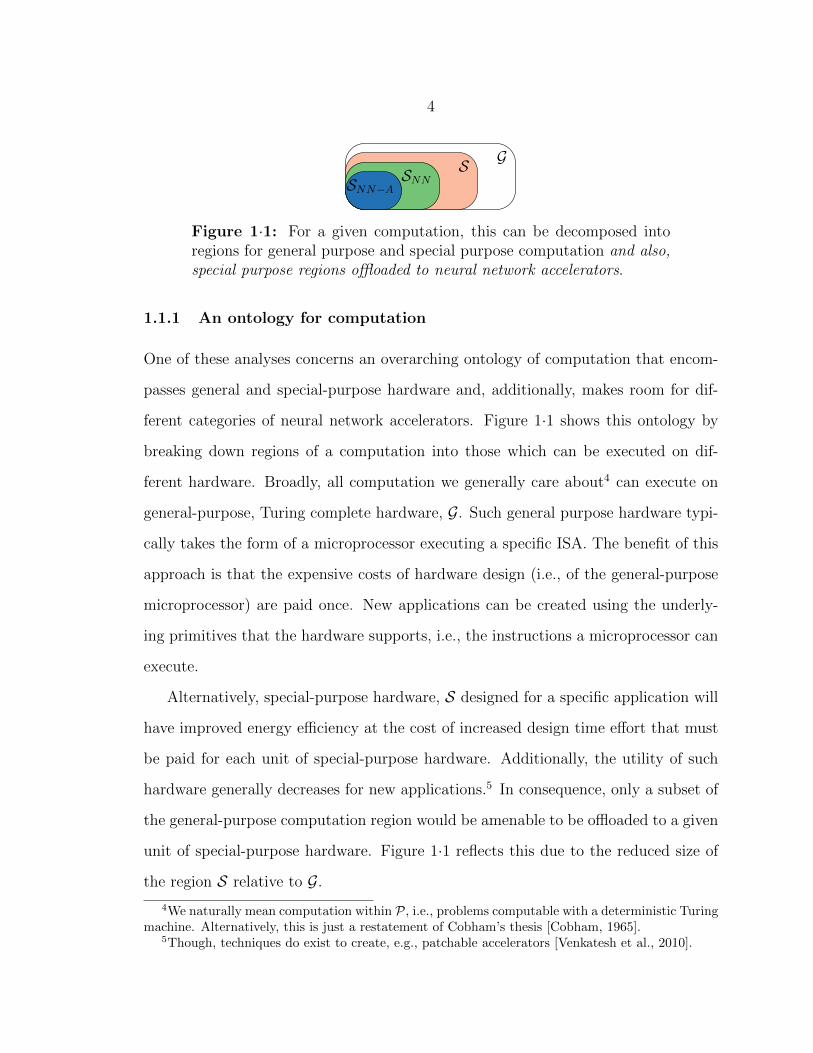
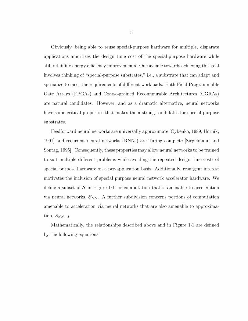
Figure 1·1: For a given computation, this can be decomposed intoregions for general purpose and special purpose computation and also,special purpose regions offloaded to neural network accelerators.
1.1.1 An ontology for computation
One of these analyses concerns an overarching ontology of computation that encom-
passes general and special-purpose hardware and, additionally, makes room for dif-
ferent categories of neural network accelerators. Figure 1·1 shows this ontology by
breaking down regions of a computation into those which can be executed on dif-
ferent hardware. Broadly, all computation we generally care about4 can execute on
general-purpose, Turing complete hardware, G. Such general purpose hardware typi-
cally takes the form of a microprocessor executing a specific ISA. The benefit of this
approach is that the expensive costs of hardware design (i.e., of the general-purpose
microprocessor) are paid once. New applications can be created using the underly-
ing primitives that the hardware supports, i.e., the instructions a microprocessor can
execute.
Alternatively, special-purpose hardware, S designed for a specific application will
have improved energy efficiency at the cost of increased design time effort that must
be paid for each unit of special-purpose hardware. Additionally, the utility of such
hardware generally decreases for new applications.5 In consequence, only a subset of
the general-purpose computation region would be amenable to be offloaded to a given
unit of special-purpose hardware. Figure 1·1 reflects this due to the reduced size of
the region S relative to G.
4We naturally mean computation within P, i.e., problems computable with a deterministic Turingmachine. Alternatively, this is just a restatement of Cobham’s thesis [Cobham, 1965].
5Though, techniques do exist to create, e.g., patchable accelerators [Venkatesh et al., 2010].
5
Obviously, being able to reuse special-purpose hardware for multiple, disparate
applications amortizes the design time cost of the special-purpose hardware while
still retaining energy efficiency improvements. One avenue towards achieving this goal
involves thinking of “special-purpose substrates,” i.e., a substrate that can adapt and
specialize to meet the requirements of different workloads. Both Field Programmable
Gate Arrays (FPGAs) and Coarse-grained Reconfigurable Architectures (CGRAs)
are natural candidates. However, and as a dramatic alternative, neural networks
have some critical properties that makes them strong candidates for special-purpose
substrates.
Feedforward neural networks are universally approximate [Cybenko, 1989, Hornik,
1991] and recurrent neural networks (RNNs) are Turing complete [Siegelmann and
Sontag, 1995]. Consequently, these properties may allow neural networks to be trained
to suit multiple different problems while avoiding the repeated design time costs of
special purpose hardware on a per-application basis. Additionally, resurgent interest
motivates the inclusion of special purpose neural network accelerator hardware. We
define a subset of S in Figure 1·1 for computation that is amenable to acceleration
via neural networks, SNN . A further subdivision concerns portions of computation
amenable to acceleration via neural networks that are also amenable to approxima-
tion, SNN−A.
Mathematically, the relationships described above and in Figure 1·1 are defined
by the following equations:
6
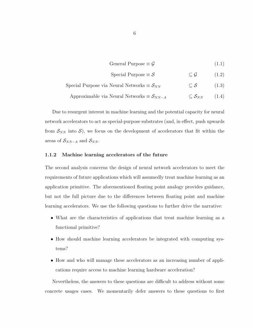
General Purpose ≡ G (1.1)
Special Purpose ≡ S ⊆ G (1.2)
Special Purpose via Neural Networks ≡ SNN ⊆ S (1.3)
Approximable via Neural Networks ≡ SNN−A ⊆ SNN (1.4)
Due to resurgent interest in machine learning and the potential capacity for neural
network accelerators to act as special-purpose substrates (and, in effect, push upwards
from SNN into S), we focus on the development of accelerators that fit within the
areas of SNN−A and SNN .
1.1.2 Machine learning accelerators of the future
The second analysis concerns the design of neural network accelerators to meet the
requirements of future applications which will assumedly treat machine learning as an
application primitive. The aforementioned floating point analogy provides guidance,
but not the full picture due to the differences between floating point and machine
learning accelerators. We use the following questions to further drive the narrative:
• What are the characteristics of applications that treat machine learning as a
functional primitive?
• How should machine learning accelerators be integrated with computing sys-
tems?
• How and who will manage these accelerators as an increasing number of appli-
cations require access to machine learning hardware acceleration?
Nevertheless, the answers to these questions are difficult to address without some
concrete usages cases. We momentarily defer answers to these questions to first

7
discuss general-purpose and special-purpose hardware in light of recent, novel uses of
machine learning.
1.2 Motivating Applications
Two recent applications of machine learning, approximate computing via function
approximation [Esmaeilzadeh et al., 2012b, Amant et al., 2014, Moreau et al., 2015]
and automatic parallelization [Waterland et al., 2012, Waterland et al., 2014], employ
neural networks in untraditional ways. Specifically, they utilize machine learning to
augment and improve the energy efficiency of existing applications.
Neural networks can be used to approximate functions and, to maximize energy
efficiency gains, approximated functions should be hot, i.e., frequently used. Put
broadly, a user or compiler profiles or injects code to build up an approximate model
of some region of code. That region of code can then be replaced with an approx-
imate version. Dynamic programming/memoization is a classical, non-approximate
technique that uses a similar approach. While existing work in this area approxi-
mates compiler-identified hot regions in handpicked benchmarks, the obvious place
to look for hot functions is in shared code. Such shared code, assumedly packaged
into shared libraries, introduces an interesting opportunity for neural network accel-
erator hardware. Specifically, since neural networks are then approximating shared
functions, the constituent neural networks backing this approximation must also be
shared. This introduces the first requirement of future neural network accelerators,
namely the capacity for sharing descriptions of neural networks across requests.
In automatic parallelization work, neural networks predict future microprocessor
state.6 Spare system resources then speculate based on these predictions. As a
6 For readers with a hardware design background, this work can appear relatively opaque. Ahelpful analogy is to view this work as a generalization of branch prediction (where a single bitof state is predicted) to multiple bits. The predicted bits, however, can exist anywhere in the fullstate of the microprocessor (architectural state, registers, memory). This work hinges on choosing
8
hedging mechanism and to improve performance, multiple predictions from a given
state are made. In consequence, many requests to access neural network resources
are generated at the same time. Similarly, as aforementioned approximate computing
work (or, more generally, machine learning) becomes more prominent, many different
processes may begin using the neural network accelerator resources of a system. This
introduces the second requirement of future neural network accelerators, namely the
capability to manage multiple simultaneous requests within short time frames. A
further, tangential benefit is the capability to exploit multiple requests to neural
network accelerator resources, e.g., to improve accelerator throughput.
These two applications demonstrate future directions for the use of machine learn-
ing and neural networks in applications. Specifically, machine learning augments and
benefits applications which were originally characterized as having no relation to ma-
chine learning. This directly contrasts with the current viewpoint where machine
learning is the application. While obviously extrapolatory, this viewpoint mirrors the
transition of floating point hardware from the realm of “scientific architectures” to
everyday computing systems, e.g., mobile phones. This transition requires a rethink-
ing of neural network accelerator hardware, as well as user and operating system
software, that integrates and manages both neural network sharing and requests to
access accelerator resources.
Not surprisingly, this dissertation applies a holistic, system-level view to neural
network computing that spans the software and hardware stack. Motivated by appli-
cations like approximate computing via neural networks and automatic paralleliza-
tion, we design accelerator hardware and software to support such new applications.
Specifically, we incorporate accelerator hardware alongside a traditional micropro-
points in an executing program where small numbers of bits change, e.g., at the top of loops. Froma mathematical view, this work views a microprocessor as a dynamical system where points withsmall Hamming distances along the trajectory are predicted using machine learning. Approximatepredictions of state can still be useful.
9
cessor and include a full discussion of the user and supervisor (operating system)
software necessary to support future machine learning accelerators.7
1.3 Outline of Contributions
1.3.1 Thesis statement
Broadly, a multi-context, multi-transaction model of neural network computation has
the following benefits:
1. It aligns with the needs of modern, highly novel, and emerging applications that
utilize machine learning as an application primitive, for learning and prediction,
on top of which complex applications can be built.
2. Such a model can be achieved with low overhead while improving the overall
throughput of a backend accelerator matching this multi-transaction model.
3. The necessary management infrastructure for a multi-transaction model, both
hardware and software, can be sufficiently decoupled from the backend acceler-
ator such that multiple backends can be supported.
4. All hardware and software for such a model can be realized and integrated with
an existing general-purpose software and hardware environment.
Nevertheless, the benefits of a multi-transaction model are predicated on two
assertions. First, there exists sufficiently interesting work that can be achieved with
“small” neural networks, on the order of tens to hundreds of neurons, such that a
multi-transaction model can realize significant throughput improvements.8 Second,
7It is our opinion that such a system-level view is generally necessary when thinking aboutnon-trivial accelerators. Specifically, how will the user access an accelerator? How will the oper-ating system manage the accelerator? What data structures need to be maintained across contextswitches?
8Small neural networks have the potential for the most dramatic throughput gains in a multi-transaction model due to the large number of data dependencies as a portion of the total numberof computations required to execute the network.
10
a neural network accelerator meeting the requirements outlined above does, in fact,
exist and can be realized.
Towards validating these assertions, we present two bodies of work. First, we
explore the design and implementation of an accelerator architecture for specific, fixed
topology neural networks. This accelerator enables fine-grained approximation of
mathematical functions in a shared library using small networks. Second, leveraging
lessons learned from this first accelerator, we design a new accelerator capable of
processing multiple neural network transactions simultaneously.
In experimental support of the aims of this thesis and towards validating the ben-
efits of our multi-transaction model, we provide and evaluate this second accelerator
implementation as well as its hardware and software integration with an open source
microprocessor and operating system. We experimentally evaluate this accelerator on
energy efficiency grounds and, expectedly, find dramatic gains over software. Further-
more, the accelerator improves its throughput with additional transactions validating
our multi-transaction model.
1.3.2 Contributions
Our design and implementation of a fixed topology neural network accelerator, T-
fnApprox, applies function approximation at very small functional granularities,
specifically transcendental functions. This work does not address the previous is-
sues of sharing and management of multiple transactions, but serves as an example
implementation of a neural network accelerator. This work then further motivates,
by counterexample, the need for a system-level view of neural network acceleration.
Additionally, this work empirically reiterates a rough lower bound on the amount
of computation that can be approximated using digital neural network accelerator
hardware.
Our proposed arbitrary topology neural network accelerator supporting both neu-
11
ral network sharing and a multi-transaction model comprises three specific contribu-
tions. First, we provide an example MLP neural network accelerator backend called
DANA (a Dynamically Allocated Neural Network Accelerator). DANA uses a Pro-
cessing Element (PE) model (similar to recent MLP accelerators in the approximate
computing literature [Esmaeilzadeh et al., 2012b, Moreau et al., 2015]). However, in
contrast to existing work, DANA does not execute a stored program implementing
a neural network, but uses a binary data structure describing a neural network—
what we refer to as a neural network configuration. DANA then can be viewed as a
control unit capable of scheduling the constituent neurons described by a neural net-
work configuration on its PEs. This model enables us to naturally support multiple
transactions via the interleaving of neurons from outstanding requests.
Second, we provide hardware and software support for managing requests to ac-
cess a backend neural network accelerator (with DANA being one example of such
a backend). This infrastructure, X-FILES, comprises a set of hardware and software
Extensions for the Integration of Machine Learning in Everyday Systems.9 On the
hardware side, we detail an X-FILES Hardware Arbiter that manages transactions,
i.e., requests to access DANA. We interface X-FILES/DANA as a coprocessor of a
Rocket RISC-V microprocessor developed at UC Berkeley [UC Berkeley Architecture
Research Group, 2016]. We then provide an X-FILES user software library that appli-
cation developers can use to include neural network transactions in their software. We
provide two sets of supervisor software: one that interfaces with a basic uniprocess-
ing kernel developed at UC Berkeley called the Proxy Kernel [RISC-V Foundation,
2016b] and another that provides support for the Linux kernel.
Together, this system comprises Rocket + X-FILES/DANA, i.e., a Rocket micro-
processor with an X-FILES transaction manager and a DANA accelerator. Finally we
9We beseech the reader to forgive the acronyms—no FOX, SKINNER, or CGB SPENDER cur-rently exist.
12
evaluate Rocket + X-FILES/DANA using power and performance criteria on single
and multi-transaction workloads. All work related to X-FILES/DANA is provided
under a 3-clause Berkeley Software Distribution (BSD) license on our public GitHub
repository [Boston University Integrated Circuits and Systems Group, 2016].
In summary, the specific contributions of this dissertation are as follows:
• A fixed topology neural network accelerator architecture used for transcendental
function approximation, T-fnApprox, that demonstrates the limits of function
approximation techniques using digital accelerators [Eldridge et al., 2014]
• An architectural description of DANA, an arbitrary topology neural network ac-
celerator architecture capable of processing multiple neural network transactions
simultaneously [Eldridge et al., 2015]
• An architectural description of the X-FILES Hardware Arbiter, a hardware
transaction manager that facilitates scheduling of transactions on a backend
(of which DANA is provided as an example)
• A description of user and supervisor software necessary to facilitate the manage-
ment of transactions on the X-FILES Hardware Arbiter from both a user and
kernel perspective
• An evaluation of Rocket + X-FILES/DANA across the design space of X-
FILES/DANA and on single and multi-transaction workloads
1.4 Dissertation Outline
This dissertation is organized in the following manner. Section 2 details the history
of neural networks as well as the copious work in this area related to hardware ac-
celeration of neural networks and machine learning algorithms. Section 3 provides
a description and evaluation of T-fnApprox, a fixed topology architecture used for
13
mathematical function approximation. The limitations of this architecture are high-
lighted. Section 4 describes the X-FILES, hardware and software that enables the safe
use of neural network accelerator hardware by multiple processes. Section 5 describes
the architecture of our arbitrary topology neural network accelerator architecture,
DANA, that acts as a backend accelerator for the X-FILES. Section 6 evaluates X-
FILES/DANA, integrated with a RISC-V microprocessor on power and performance
metrics. In Section 7, we conclude and discuss observations and future directions for
this and related work.
14
Chapter 2
Background
2.1 A Brief History of Neural Networks
The history of neural networks, artificial intelligence, and machine learning1 is an
interesting study in and of itself largely due to the fact that this history is dotted
with proponents, detractors, significant advances, and three major waves of disap-
pointment and associated funding cuts.2 While not specifically necessary for the un-
derstanding of this dissertation or its contributions, we find that having some broad
perspective on the history of neural networks provides the reader with necessary
grounding that has unfortunately contributed to much of the past disappointment in
neural networks as computational tools over the past seven decades.
2.1.1 Neural networks and early computer science
The human brain or, much more generally, any cortical tissue has long been viewed
as an inspirational substrate for developing computing systems. Put simply, humans
and animals perform daily tasks which can be classified as computation (e.g., logical
inference, mathematics, navigation, and object recognition) and they are exceedingly
good at these tasks. Furthermore, these biological substrates are the result of millions
of years of evolution lending credence to the belief that these substrates are, at worst,
1We view these names as interchangeable—they all refer to similar aspects of the same underlyingproblem: How do we design machines capable of performing human-level feats of computation? Thenaming convention, historically, is largely an artifact of the research and funding climate at the time.
2These waves of disappointment are generally referred to hyperbolically as AI winters.
15
suitable and, more likely, highly optimized. It is therefore reasonable to expect that
such biological substrates provide guideposts towards developing machines capable
of similar computational feats. Unsurprisingly, psychological and biological devel-
opments motivated and shaped the views of the emerging area of computer science
during the early 20th Century.
Unfortunately, though perhaps unsurprisingly, the human brain is a highly com-
plex organ whose mechanisms are exceedingly difficult to discern.3 Nevertheless, cor-
tical tissue does demonstrate some regular structure. Namely, such tissue is composed
of interconnected elementary cells, neurons, that communicate through electrical and
chemical discharges, synapses, that modify the electrical potential of a neuron.
While the full computational properties of biological neurons are complex and not
completely understood,4 neurons generally demonstrate behavior as threshold units:
if the membrane potential, the voltage of the neuron augmented by the summation of
incident connections, exceeds a threshold, the neuron generates a spike to its outgoing
connected neurons. McCulloch and Pitts provide an axiomatic description of an
artificial neuron in this way [McCulloch and Pitts, 1943].
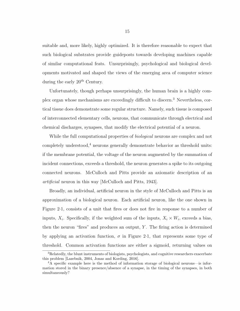
Broadly, an individual, artificial neuron in the style of McCulloch and Pitts is an
approximation of a biological neuron. Each artificial neuron, like the one shown in
Figure 2·1, consists of a unit that fires or does not fire in response to a number of
inputs, Xi. Specifically, if the weighted sum of the inputs, Xi ×Wi, exceeds a bias,
then the neuron “fires” and produces an output, Y . The firing action is determined
by applying an activation function, σ in Figure 2·1, that represents some type of
threshold. Common activation functions are either a sigmoid, returning values on
3Relatedly, the blunt instruments of biologists, psychologists, and cognitive researchers exacerbatethis problem [Lazebnik, 2004, Jonas and Kording, 2016].
4A specific example here is the method of information storage of biological neurons—is infor-mation stored in the binary presence/absence of a synapse, in the timing of the synapses, in bothsimultaneously?
16
W1 W2 W3 W4W5
X1 X2 X3 X4 X5 bias
σ
(∀ inputs∑i
Xi ×Wi + bias
)
Y
Figure 2·1: A single artificial neuron with five inputs
range [0, 1], or a hyperbolic tangent, returning values on range [−1, 1]. Other options
include rectification using a ramp or softplus function to produce an unbounded
output on range [0,∞].
Critically, McCulloch and Pitts also demonstrated how assemblies of neurons can
be structured to represent logic functions (e.g., Boolean AND and OR gates), storage
elements, and, through the synthesis of logic and storage, a Turing machine. Later
work by Frank Rosenblatt solidified the biological notion of receptive fields, i.e., groups
of neurons, here termed perceptrons, producing different behavior based on their local
regions of activation [Rosenblatt, 1958]. The resulting body of work derived from and
related to this approach is termed connectionism.
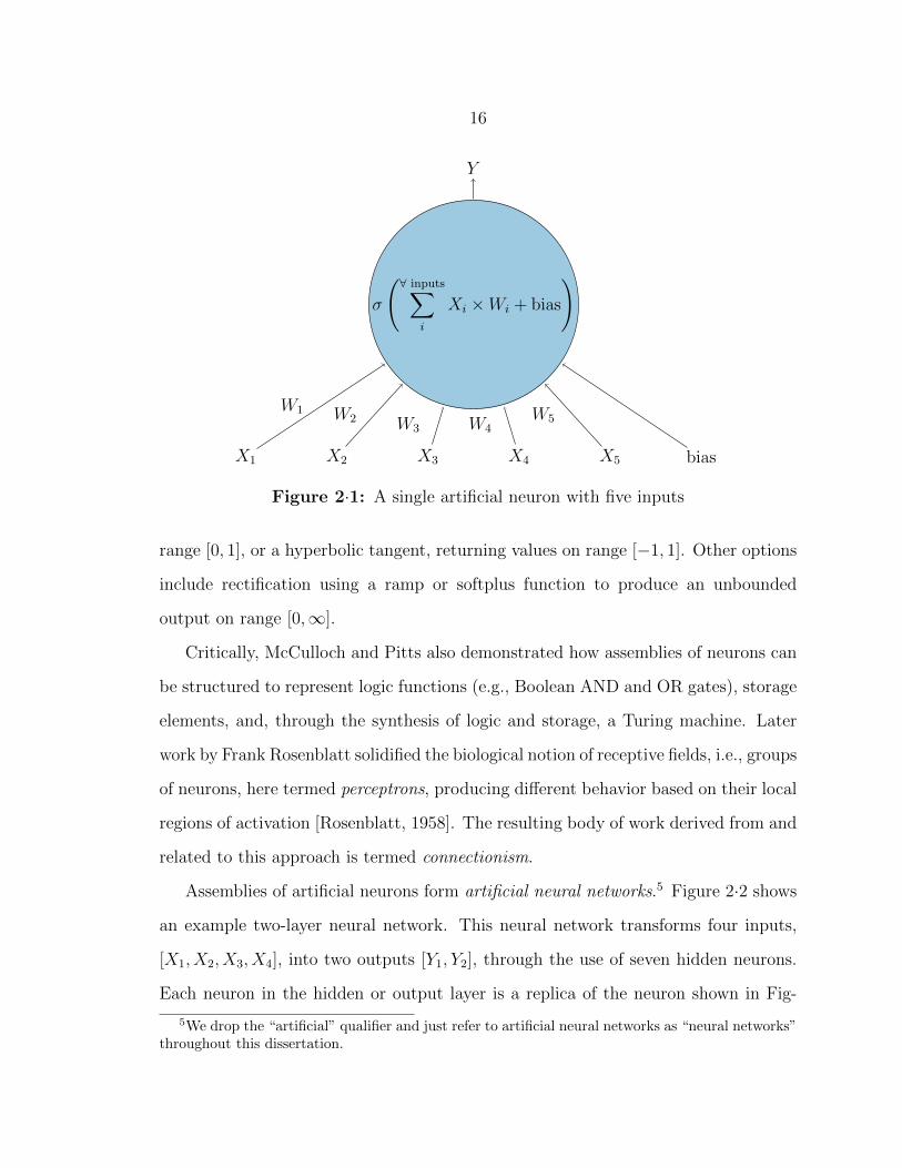
Assemblies of artificial neurons form artificial neural networks.5 Figure 2·2 shows
an example two-layer neural network. This neural network transforms four inputs,
[X1, X2, X3, X4], into two outputs [Y1, Y2], through the use of seven hidden neurons.
Each neuron in the hidden or output layer is a replica of the neuron shown in Fig-
5We drop the “artificial” qualifier and just refer to artificial neural networks as “neural networks”throughout this dissertation.
17
X1 X2 X3 X4
bias
bias
Y1 Y2
HiddenLayer
InputLayer
OutputLayer
Figure 2·2: A two layer neural network with four inputs and threeoutputs
ure 2·1. Note that the neurons in the input layer are pass-through and do not modify
their inputs. Through careful selection of weights, the neural network can be made
to approximate a general input–output relationship or, much more simply and stated
previously, arbitrary Boolean functions or collections of Boolean functions.
This fact was not lost on early pioneers of computer science who drew heavy in-
spiration from biological neurons when designing early computers.6 In fact, it seemed
only natural that neurons should form the basis of computing. Neurons could act like
logic gates and Claude Shannon had already demonstrated the equivalence of existing
digital circuit elements and Boolean logic [Shannon, 1938]. Qualitatively, John von
Neumann specifically refers to the work of McCulloch and Pitts in his technical notes
on the design of the EDVAC [von Neumann, 1993].7 However, and more interestingly,
6Similarly, this notion of neurons as Boolean functions coincidentally or causally aligns with theearly 20th Century focus on the philosophy and foundation of mathematics with particular focus onLogicism, i.e., the efforts of Betrand Russel and Alfred North Whitehead to reduce mathematics tologic [Whitehead and Russell, 1912]. Granted, later proofs by Kurt Godel make this line of thoughtless convincing and even intractable.
7The Electronic Discrete Variable Automatic Computer was a bit serial computer developed forthe United States Army’s Ballistics Research Laboratory at the Aberdeen Proving Ground and apredecessor of the more well known ENIAC.

18
this biological motivation is implicit in von Neumann’s descriptions of computational
units as “Organs”, the bit serial architecture of the EDVAC, and even in the very
figures that von Neumann uses to describe the computational organs as assemblies
of neurons. Similar sentiments, and almost entirely biologically-inspired designs, are
presented again by von Neumann when he discusses approaches to build reliable
computing systems [von Neumann, 1956]. Relatedly, Alan Turing commented exten-
sively on the philosophical struggle of what it truly means for a machine to “think”,
i.e., reproduce the computational capabilities of the brain in a way indistinguishable
to a human observer [Turing, 1950]. Programmatic approaches to general-purpose
learning by machines, with psychological influences, can be seen by the concept of
memoization as proposed by Donald Michie [Michie, 1968]. Here a machine (or a
human), performs some action by rote memorization (e.g., via top-down dynamic
programming) or by some rule (e.g., an algorithm).
In short, it is exceedingly difficult, though likely unnecessary, to decouple the pre-
dominant biological computing substrate, the brain, from artificial computing sub-
strates. However, as this area of research progressed, traditional computing with
logic gates as the primitives broke off from connectionist approaches that aligned
with artificial intelligence efforts.
2.1.2 Criticisms of neural networks and artificial intelligence
Nevertheless, this emerging area of artificial intelligence proceeded with fits and starts
and notable high profile criticism.
First, Hubert Dreyfus, working for RAND corporation, provided a stark criti-
cism of artificial intelligence research. Dreyfus’ report questioned the fundamental
assumptions of the brain as hardware and the mind as software [Dreyfus, 1965].8 Put
8It is interesting to note that the very title of this work, “Alchemy and Artificial Intelligence,”draws parallels to modern work on deep neural networks—the networks are not fully understoodand the construction and training of these networks is viewed as a black art.
19
simply, much of the research into building a machine with artificial intelligence hinges
on the tenuous assumption that the brain, hardware, is a collection of neurons act-
ing as logic gates and the mind, software, is either the organization or the program
running on the hardware. However, just because neurons (or artificial representa-
tions of neurons) can be constructed in such a way that they behave like logic gates
does not mean that this is the only function of neurons. Analogously, transistors,
either metal-oxide-semiconductor field-effect-transistors (MOSFETs) or bipolar junc-
tion transistors (BJTs), can be arranged to behave like logic gates. However, this
does not mean that such behavior encompasses the underlying physics or information
processing capabilities of transistors.
Second, and most often recalled, Marvin Minsky and Seymour Papert published
Perceptrons in 1969 that provided bounds on the fundamental computational limits
of neurons [Minsky and Papert, 1987]. Specifically, and famously, Minksy describes
the scenario of a single neuron, like that of Figure 2·1, being incapable of learning an
XOR relationship due to the fact that this representation is not linearly separable.
In effect, a single neuron is not a universal logic gate. Granted, the obvious counter
criticism is that neural networks composed of more than one neuron in series can
learn an XOR function. Nevertheless, this observation led to a decrease in interest in
connectionist architectures.
Third, Sir James Lighthill provided a scathing critique of current artificial intelli-
gence research with the dramatic effect being that the United Kingdom scaled back all
research in this area [Lighthill, 1973]. Briefly, it is worth mentioning Lighthill’s classi-
fication of AI research as it bears similarities to the continued difficulties and problems
of research in the field (or machine learning/neural networks) today. Lighthill groups
AI research into three main areas:
Improved Automation (class A) Work in this area encompasses improvements

20
to traditional techniques of object recognition, natural language processing, and
similar topics. This work is relatively easy to evaluate as it can be compared
directly against the best existing traditional approach that does not have any
grounding in biology.
Cognitive Neuroscience (CNS) Research assisted by a Computer (class C)
CNS research can be augmented and enhanced by the use of computers through
the simulation of biological systems, e.g., neurons. Additionally, this allows for
fundamental psychological concepts to be tested with assemblies similar to or
inspired by biology.
Bridge Activities, chiefly Robotics (class B) This work attempts to combine
fundamental CNS research with improved automation and often takes the form
of, as Lighthill somewhat derogatorily calls, “building robots.”
The identified split between Lighthill’s A and C classes largely persists to this day.
Fundamental advances in neural networks and machine learning has enabled dramatic
improvements in automation, e.g., image classification. Similarly, the ability of models
of the cortical tissue of the human or animal brain to be simulated in computer
software or hardware allows for new insights to be gleaned in both neuroscience and
psychology. However, the combination of these two research areas still leaves much
to be desired. Put differently, biological inspiration cannot be a beneficial criteria
in its own right or, similarly, adopting a biologically-inspired approach is no explicit
guarantee of success.9 Nevertheless, there is no reason to not take inspiration from
biology ! The expectations, however, must be tempered appropriately. Furthermore,
the lack of tempered expectations, promises, and restraint by researchers can be
viewed as a dominant cause in the repeated periods of disenfranchisement with neural
9This is something which I learned the hard way through an experiment involving a hardwareimplementation of a biologically-inspired approach to optical flow [Raudies et al., 2014]. Whileinteresting in its own right, such work was unable to achieve comparable performance to a state ofthe art traditional, i.e., a non-biologically-inspired, approach.
21
networks.
In combined effect, these criticisms diminished interest (and funding) in connec-
tionist approaches to artificial intelligence, i.e., approaches involving groupings of
neurons into larger assemblies, until their resurgence in the 1990s.
2.1.3 Modern resurgence as machine learning
Following the initial downfall of connectionist approaches, the 1980s commercial ar-
tificial intelligence market was dominated by expert systems and Lisp machines that
aimed to describe the world with rules. Nevertheless, these systems and their asso-
ciated companies were largely defunct by the 1990s. However, the reemergence of
connectionist approaches can be seen during the 1980s and, generally, as a continua-
tion of computing by taking inspiration from biology.
While the work of McCulloch and Pitts as well as Rosenblatt provided some
biological grounding for artificial intelligence, Hubel and Wiesel provided a concrete
model for how the visual processing system operates. In their work on the cat visual
cortex, they demonstrated that certain cells are sensitive to points over specific regions
of the retina, i.e., the receptive fields of Rosenblatt [Rosenblatt, 1958]. Further along
in the visual processing system, other cells are sensitive to lines (collections of points)
and still others to collections of lines or specific motions [Hubel and Wiesel, 1965]. Put
simply, biological visual processing systems are hierarchically organized and construct
complex structures from simpler primitives.
Fifteen years later, a more concrete structure for a generic connectionist architec-
ture inspired by the visual processing system as experimentally determined by Hubel
and Wiesel emerged—the work on the Neocognitron by Fukushima [Fukushima, 1980].
Additionally, evidence and techniques that allowed neural networks to be incremen-
tally modified through error backpropagation to represent an arbitrary input–output
relationship [Rumelhart et al., 1988] reignited significant interest in connectionism.
22
Nevertheless, approaches were plagued by the so-called vanishing gradient problem
where the gradient decreases exponentially with the number of layers in a network.
In result, the features used by an architecture like the Neocognitron had to be hand
selected and could not be generally learned.
A number of approaches towards dedicated neural network computers or hard-
ware to enable neural network computation in the 1990s [Fakhraie and Smith, 1997].
However, the lineage of Hubel and Wiesel to Fukushima and general research into con-
nectionist approaches to artificial intelligence were maintained and furthered during
this time by the so-called Canadian mafia: Yann LeCun, Geoff Hinton, and Yoshua
Bengio. LeCun provided prominent work into convolutional neural networks, i.e.,
neural networks inspired by the visual processing system that use convolutional ker-
nels as feature extractors (whose size effectively defines a receptive field), and their
training [Lecun et al., 1998]. Similarly, Hinton provided a means of training another
type of deep neural network—a deep belief network composed of stacked Restricted
Boltzmann Machines—using a layer-wise approach [Hinton et al., 2006]. This work,
and followup work in this area, provide a means of avoiding the vanishing gradient
problem through connectivity restrictions or layer-wise training and demonstrated
the capabilities of connectionist approaches to solve difficult problems: image classi-
fication and scene segmentation.
In consequence, these successes, and numerous ones since, have created a dra-
matically increased and resurgent interest in machine learning. However, the general
utility of machine learning is not in its ability to solve a specific niche problem, e.g.,
image classification. Machine learning provides a general class of substrates, neural
networks and their variants, for automatically extracting some structure in presented
data. This contrasts dramatically with traditional, algorithmic computing where a
complete understanding of a specific problem is required. Instead, machine learning
23
Table 2.1: Related work on neural network software and hardware
Category Work Citation
Software Libraries
FANN [Nissen, 2003]Theano [Al-Rfou et al., 2016]Caffe [Jia et al., 2014]cuDNN [Chetlur et al., 2014]Torch [Collobert et al., ]Tensorflow [Abadi et al., 2015]
Spiking Hardware SpiNNaker [Khan et al., 2008]TrueNorth [Preissl et al., 2012]
Hardware Architecture
RAP [Morgan et al., 1992]SPERT [Asanovic et al., 1992]NPU [Esmaeilzadeh et al., 2012b]NPU–Analog [Amant et al., 2014]DianNao [Chen et al., 2014a]DaDianNao [Chen et al., 2014b]NPU–GPU [Yazdanbakhsh et al., 2015]PuDianNao [Liu et al., 2015]SNNAP [Moreau et al., 2015]TABLA [Mahajan et al., 2016]DNNWEAVER [Sharma et al., 2016]
FPGA Hardware HMAX-FPGA [Kestur et al., 2012]ConvNet [Farabet et al., 2013]
can be viewed as a soft computing paradigm where approximate or inexact solutions
are served for problems with no known algorithmic (or non NP-hard) solution is
currently known.
2.2 Neural Network Software and Hardware
The long tail of neural network research and modern, resurgence interest has resulted
in a wide array of historical and recent software and hardware for performing and
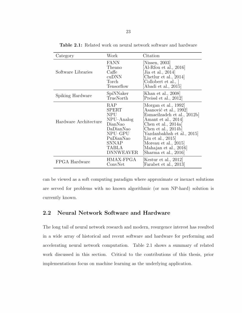
accelerating neural network computation. Table 2.1 shows a summary of related
work discussed in this section. Critical to the contributions of this thesis, prior
implementations focus on machine learning as the underlying application.
24
2.2.1 Software
Machine learning software can be divided into roughly two categories:
• Software specific for machine learning
• Software for scientific (or mathematical) computation
In the former space, the Fast Artificial Neural Network (FANN) library is a repre-
sentative example [Nissen, 2003]. This is a C library (with an optional C++ wrapper)
that allows for computations with arbitrary multilayer perceptron neural networks
and training using backpropagation algorithms. However, due to the time during
which FANN was developed (i.e., 2003), this software library was optimized for a
single CPU implementation—specifically with the use of software pipelining.
More recent versions of dedicated machine learning software include Caffe [Jia
et al., 2014] and Tensorflow [Abadi et al., 2015]. In contrast with FANN, both of
these libraries target deep learning specifically, i.e., convolutional neural networks or
deep neural networks. In light of their much more recent development than some-
thing like FANN, they both target the predominant architecture for training neural
networks—GPUs. GPU programming, while initially archaic in the sense that a user
had to translate their program into an explicit graphics language, e.g., OpenGL. How-
ever, NVIDIA introduced CUDA, a C/C++-like language that enables more straight-
forward programming on the parallel architecture of a GPU, in 2007. The natural
parallelism inherent in machine learning workloads makes GPUs a prime target for
bearing the computational burdens of both feedforward inference and learning. To
further bolster their support of this, NVIDIA introduced cuDNN, deep neural net-
work (DNN) extensions to its existing CUDA library for programming GPUs [Chetlur
et al., 2014].
Alternatively, though the boundary is somewhat fuzzy, more generic scientific
computing packages can be used to describe machine learning algorithms. These
25
libraries include Theano [Al-Rfou et al., 2016] and Torch [Collobert et al., ]. Similarly,
both of these provide support for targeting both CPU and GPU backends.
Nevertheless, all of these existing software implementations treat machine learning
as the underlying application as opposed to just one more way of approaching a
problem.
2.2.2 Hardware
Hardware implementations can be broadly broken down along the guidelines of Lighthill’s
A (advanced automation) and C (cognitive neuroscience) classes. Class A imple-
mentations involve artificial neural networks which includes multilayer perceptron
and convolutional/deep implementations. Class C generally uses a spiking model
for inter-neuron computation. However, while Class C can obviously be utilized for
neuroscience simulations, these implementations often merge into Class A or B and
attempt to provide some utility for a specific application domain.
Biologically-inspired approaches include SpiNNaker [Khan et al., 2008] and IBM’s
recent entry, TrueNorth [Preissl et al., 2012]. Both use spiking neural network models
and provide a more biologically-accurate view of neural network hardware. Neverthe-
less, the general utility of these types of systems for Class A tasks is widely disputed,
e.g., in comments by Yann LeCun to the New York Times [Markoff, t B1]. Specifically,
artificial neural networks, like convolutional neural networks, tend to outperform spik-
ing models on the same tasks. While this does not preclude their use for Class A
tasks, most of these systems are relegated to Class C.
Artificial neural network hardware accelerators were explored in the 1990s, specifi-
cally with the Ring Array Processor (RAP) [Morgan et al., 1990, Przytula, 1991, Mor-
gan et al., 1992] and SPERT [Asanovic et al., 1992, Wawrzynek et al., 1996]. RAP
utilized a collection of digital signal processors (DSPs) connected via a ring bus.
Individual neurons can then be assigned to specific DSPs with broadcast communi-
26
cation for inference or learning happening over the ring bus. SPERT and SPERT-II
were both very long instruction word (VLIW) machines and were evaluated on neu-
ral network inference and learning applications demonstrating dramatic performance
improvements over IBM and SPARC workstations. Similarly, the performance (i.e.,
speed) of these systems actually improved with increases in neural network layer size.
Put differently, as more work is exposed to the underlying hardware, its performance
scales accordingly. This is a favorable quality that demonstrates the soundness of the
architecture and a feature that we have tried to replicate with the work presented in
this thesis.
Following RAP and SPERT there was little interest in hardware for connectionist-
style neural networks until the modern, resurgent interest in deep learning. In 2012,
Hadi Esmaeilzadeh demonstrated the use of classical artificial neural networks, neural
processing units (NPUs), to approximate hot regions of code for significant power–
performance savings [Esmaeilzadeh et al., 2012b]. Follow-up work extended this
to analog NPUs [Amant et al., 2014], as accelerators on a GPU [Yazdanbakhsh
et al., 2015], and as a dedicated NPU coprocessor for embedded applications called
SNNAP [Moreau et al., 2015]. The context and motivation of this work was entirely
focused on the use of NPUs to enable function approximation and developing one type
of hardware infrastructure, neural network accelerators, to enable hardware-backed
approximation of arbitrary regions of code. This is similar to related work by the
same authors on hardware modifications that allow for general approximate compu-
tation and storage using multiple voltage levels [Esmaeilzadeh et al., 2012a]. All of
this work is intended to operate using a language which allows for approximate types
like EnerJ [Sampson et al., 2011].
Neural network hardware, primarily focused on deep/convolutional networks, be-
gan to reemerge recently. This work has generally taken the form of architecture
27
research or dedicated hardware accelerators, sometimes implemented using FPGAs
or as ASICs. Specifically, FPGA hardware implementations have been developed
for both hierarchical model and X (HMAX) [Kestur et al., 2012] and convolutional
neural networks [Farabet et al., 2013]. Related attempts have been made to sim-
plify the design process of emitting an implementation of a specific neural network
accelerator into a hardware substrate, e.g., an FPGA. TABLA (correctly) identifies
gradient descent as the common algorithm across which a multitude of statistical
machine learning approaches can be implemented [Mahajan et al., 2016]. TABLA
then provides a variety of templates that can be stitched together on an FPGA to
create a machine learning accelerator. Similarly, DNNWEAVER provides templates
for creating an FPGA implementation of a machine learning accelerator, but strictly
for feedforward inference [Sharma et al., 2016].
Dedicated ASIC implementations have also been provided by the DianNao accel-
erator [Chen et al., 2014a] and its followup variants DaDianNao [Chen et al., 2014b]
and PuDianNao [Liu et al., 2015]. Note the reported performance of these implemen-
tations match or moderately exceed the performance of machine learning executing
on a GPU. However, these implementations are several orders of magnitude more
energy efficient.
In summary, the space of neural network hardware is extremely packed and com-
petitive due to recent resurgent interest in machine learning. However, all of these
systems view machine learning as the underlying application. In light of the motiva-
tions of this thesis, we view machine learning hardware as one component of systems
that enable and expose machine learning acceleration as a generic component of ar-
bitrary applications that would not traditionally use machine learning techniques.
28
Software Hardware
Generality
SpecialityFANN
Caffe
TensorFlow
Torch
Theano
TrueNorth
SpiNNaker
DianNao
PuDianNao
DaDianNao
NPU
NPU–Analog
NPU–GPUSNNAP
TABLA
DNNWEAVER
RAP
SPERT
HMAX-FPGA
ConvNet
cuDNN
X-FILES
DANA
T-fnApprox
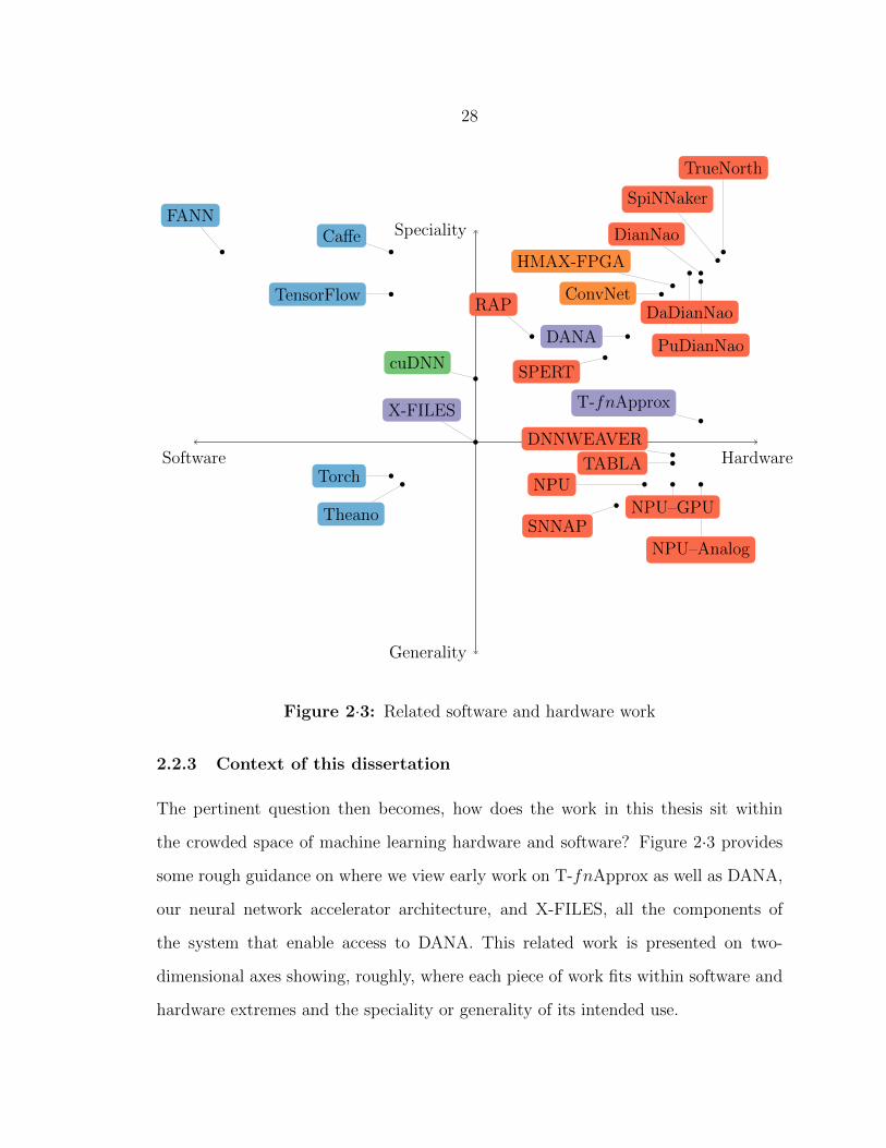
Figure 2·3: Related software and hardware work
2.2.3 Context of this dissertation
The pertinent question then becomes, how does the work in this thesis sit within
the crowded space of machine learning hardware and software? Figure 2·3 provides
some rough guidance on where we view early work on T-fnApprox as well as DANA,
our neural network accelerator architecture, and X-FILES, all the components of
the system that enable access to DANA. This related work is presented on two-
dimensional axes showing, roughly, where each piece of work fits within software and
hardware extremes and the speciality or generality of its intended use.

29
Software generally falls into categories of strictly used for neural network compu-
tation (FANN, Caffe, and TensorFlow) and more general-purpose scientific computing
packages (Torch and Theano). Recently, NVIDIA’s cuDNN has provided tight, fast
support for machine learning on one or more GPUs and has bridged the hardware/-
software gap between software neural network libraries and GPU backends. Conse-
quently, Caffe, TensorFlow, Torch, and Theano all support cuDNN bringing them
closer to hardware acceleration.
All remaining work discussed falls into the hardware hemisphere, but provides
variations on both speciality of use and software support. Biologically-inspired ap-
proaches, SpiNNaker and TrueNorth, are viewed as highly specialized models of bio-
logical systems to maintain consistency with Lighthill’s Class C grouping. Similarly,
dedicated ASIC approaches, like DianNao and its variants are similarly restricted in
their ability to adapt to the constantly changing landscape of machine learning tech-
niques. FPGA approaches, like HMAX and ConvNet, are relatedly narrow in scope.
RAP and SPERT and provided due to their historical context, but both provide
software infrastructure for programming these processors.
NPU and its variants and SNNAP both push towards the generality end of the
spectrum in that the focus of this work is not on neural network acceleration, but
using neural networks to augment traditional computation. However, the focus of
this work is specific to function approximation and there are certain problems that
are either not amenable to approximation or that are not uniquely suited to being
viewed as an input–output relationship.10 T-fnApprox lives in the same domain as
NPU work, but attempts to push the bounds on the granularity of approximation
10It is interesting to contrast this approach with Google Deepmind’s Neural Turing Machine workwhere neural networks (or LSTMs) are augmented with dedicated read/write memory to better learnan algorithm [Graves et al., 2014]. In this scenario, an architecture that includes dedicated memorycan potentially provide a much better “understanding” of an input output relationship through analgorithm as opposed to a function.
30
suitable using neural networks as function approximators. X-FILES/DANA work
differs from NPU and its variants in that we are agnostic of the way in which the
neural network hardware is used, but can definitely support neural network-backed
approximation approaches.
DNNWEAVER and TABLA provide viable ways forward to provide hardware-
based acceleration of machine learning approaches without being tied to a specific
architecture like with ASIC or FPGA implementation work. These techniques are
similarly agnostic to the way in which the hardware is used, but we strive to provide
a complete system that ties both hardware and software together with user and super-
visor software. In effect, X-FILES work could be interfaced with any of these existing
approaches, hence the separation of X-FILES and DANA contributions in Figure 2·3.
X-FILES try to span the gap between software/hardware and speciality/generality,
while DANA is one example of an accelerator backend.
DANA does bear a strong similarity to existing neural network accelerator archi-
tectures that use a PE model.11 However, the dominant contributions of this work
come in how DANA and our hardware/software infrastructure, X-FILES, work to-
gether to provide neural network computation as a fundamental primitive of both
user and supervisor software.
11A PE model generally follows the inclusion of some number of PEs that can provide the function-ality of one or more neurons. Computations are then scheduled on these PEs to “execute” a neuralnetwork provided as a raw data structure describing a neural network or as explicit instructions thatthe PEs execute.

31
Chapter 3
T-fnApprox: Hardware Support for
Fine-Grained Function Approximation
using MLPs
Approximate computing trades off precision for better performance or decreased en-
ergy. Broadly, this moves computation towards using “just enough” resources as
opposed to the blunt underlying data types of microprocessors—integer or floating
point types of some fraction or multiple of the word length. One approach to approx-
imate computing allows for finely grained precision of operations using the amount
of precision actually required for a specific operation. Alternatively, neural networks
have been empirically shown to act as approximate computing substrates where a
neural network approximates precise execution over some region. Specifically, neural
networks have been used to approximate functions or regions of code [Esmaeilzadeh
et al., 2012b, Amant et al., 2014, Moreau et al., 2015, Yazdanbakhsh et al., 2015] from
a diverse range of applications, e.g., those in the AXBENCH approximate computing
benchmark suite [Yazdanbakhsh et al., 2016], as well as entire applications [Chen
et al., 2012].
Furthermore, neural networks have been mathematically shown to be both univer-
sal approximators by Cybenko [Cybenko, 1989] and Hornik [Hornik, 1991]. Addition-
ally, Siegelmann and Sontag demonstrated that RNNs1 are Turing complete [Siegel-
1RNNs are a type of neural network with cycles. One specific example includes Long Short TermMemory (LSTM) networks [Hochreiter and Schmidhuber, 1997]. RNNs contrast with multilayerperceptron or traditional artificial neural network where the communication of data is either strictly
32
mann and Sontag, 1995]. Hence, neural networks can be viewed as blank substrates
on top of which complicated and difficult problems can be mapped via a learning
algorithm.
However, identifying regions of code capable of being approximated is an open
problem. Revisiting the ontology of Section 1.1.1, these regions of code fall into
the SNN−A subset of G. At present, this is generally solved with user annotation
of possibly approximable code followed by a compiler decision as to whether or not
a specific region of code is frequently executed (i.e., the code is “hot”) and safe
to approximate. The compiler then replaces the original code region with a neural
network executed in software or offloaded to hardware. With this work, we attempt to
circumvent the problem of hot code approximation by approximating code assumed
to be hot, i.e., shared library functions. Specifically, we focus on approximation of
transcendental functions in the GNU C Library.
3.1 Function Approximation
Function approximation has a long history. For as long as numerical computation has
been used (e.g., computing artillery firing tables), some approximation of complex
functions has been necessary. Broadly, function approximation can be viewed as
using a limited amount of information to represent a more complex system. From
a mathematical view, this can be viewed from at least two contrasting perspectives:
representation by a Taylor Series and Harmonic Analysis.
A Taylor Series represents a function as an infinite sum of functions computed us-
ing successively higher derivatives of the function. This type of approach can provide
very accurate local approximation, but diverges dramatically from the true function as
the domain of the approximation increases. Alternatively, Harmonic Analysis repre-
feedforward for inference or feedback for gradient descent learning.

33
sents functions as a summation of basis sets. One specific type of Harmonic Analysis,
Fourier Analysis, represents functions by a summation of sines and cosines. Differing
from a Taylor Series approximation, a Fourier Series approximation captures global
behavior (e.g., the average value of a function) at the expense of local, high frequency
information.
Both of these approaches have implied drawbacks when a designer attempts to
produce more accurate approximations. A Taylor Series approximation requires more
terms in the Taylor series to produce a more accurate approximation over a larger
domain. Similarly, a Fourier Series approximation requires the inclusion of higher
frequency components to improve approximation accuracy. From this perspective, a
Taylor Series seems to provide limited utility as rarely are functions approximated
over tight domains.
Neural networks, while shown to be general purpose approximators, demonstrate
the same Taylor Series-like deficiencies. Namely, neural networks are highly accurate
over a local region, but require more resources (neurons) to provide an acceptable
result over a large domain.2 For approximation of operations with full-width integer
and floating point data types, approximation over a large domain is a critical necessity.
Nevertheless, there exist techniques that extend approximation from a limited
domain to an unlimited domain. In the following subsection we provide a detailed
explanation of Unified CORDIC, an existing numerical technique for function approx-
imation. Using the approach of Unified CORDIC we are then able to apply neural
network approximation of certain mathematical library functions to unbounded input
domains.
2Granted, this approach could potentially be lessened by using activation functions composed ofa basis used in Harmonic Analysis with unknown exacerbations to the non-convexity of the learningproblem.
34
3.1.1 CORDIC and Unified CORDIC
CORDIC, developed by Jack Volder while at Convair, provides an efficient way to
compute certain “difficult” mathematical functions using shifts, adds, and a table
of inverse tangents or inverse hyperbolic tangents [Volder, 1959]. This algorithm is
generally useful for small microprocessors that do not have ready access to a multi-
plier but need to compute complex functions, e.g., its original usage case was in an
airplane guidance computer. John Walther extended the algorithm in the form of
Unified CORDIC supporting additional functions and accepting inputs on arbitrary
domains [Walther, 1971]. Unified CORDIC handles arbitrary domain inputs by iden-
tifying and exploiting the fact that a bounded domain of the function can be used to
describe its unbounded counterpoint.
As a brief example, consider the sine and cosine functions shown in Figure 3·1.
Intuitively, sine and cosine are redundant due to their periodicity—knowing one sine
or cosine period gives us full knowledge of the complete signal. However, this initial
approximation can be further simplified such that we only need to know a quarter
period of sine or cosine to reconstruct them. This quarter period of sine or cosine
can then be pieced together (with use of inversion) to completely reconstruct sine or
cosine for unbounded domain inputs. Table 3.1 shows these identities mathematically
in addition to identities for logarithmic and exponential functions.
In effect, the domain agnosticity of Unified CORDIC exploits the fact that for
some mathematical functions exact knowledge over a limited domain can be used to
reconstruct the entire function. The problem of function approximation with some-
thing like CORDIC then reduces to identifying and using a simple mathematical
transformation to move the input onto the known domain, apply the function, and
scale the output. Naturally, these aforementioned simple transformations need to be
composed of operations of complexity comparable to the approximation technique
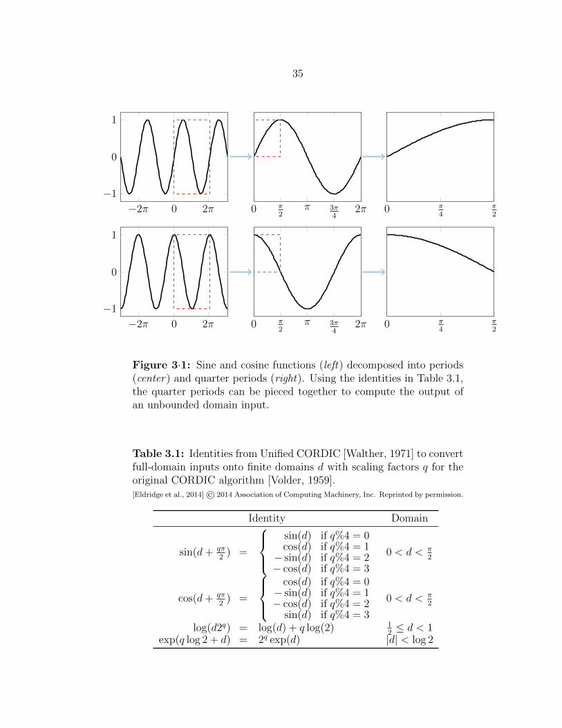
35
−2π 0 2π
−1
0
1
0 π2
π 3π4
2π 0 π4
π2
−2π 0 2π
−1
0
1
0 π2
π 3π4
2π 0 π4
π2
Figure 3·1: Sine and cosine functions (left) decomposed into periods(center) and quarter periods (right). Using the identities in Table 3.1,the quarter periods can be pieced together to compute the output ofan unbounded domain input.
Table 3.1: Identities from Unified CORDIC [Walther, 1971] to convertfull-domain inputs onto finite domains d with scaling factors q for theoriginal CORDIC algorithm [Volder, 1959].[Eldridge et al., 2014] © 2014 Association of Computing Machinery, Inc. Reprinted by permission.
Identity Domain
sin(d+ qπ2
) =
sin(d) if q%4 = 0cos(d) if q%4 = 1− sin(d) if q%4 = 2− cos(d) if q%4 = 3
0 < d < π2
cos(d+ qπ2
) =
cos(d) if q%4 = 0− sin(d) if q%4 = 1− cos(d) if q%4 = 2
sin(d) if q%4 = 3
0 < d < π2
log(d2q) = log(d) + q log(2) 12≤ d < 1
exp(q log 2 + d) = 2q exp(d) |d| < log 2
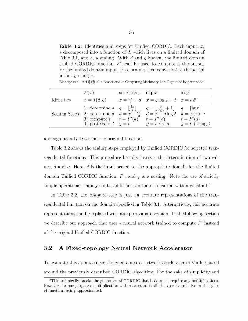
36
Table 3.2: Identities and steps for Unified CORDIC. Each input, x,is decomposed into a function of d, which lives on a limited domain ofTable 3.1, and q, a scaling. With d and q known, the limited domainUnified CORDIC function, F ′, can be used to compute t, the outputfor the limited domain input. Post-scaling then converts t to the actualoutput y using q.[Eldridge et al., 2014] © 2014 Association of Computing Machinery, Inc. Reprinted by permission.
F (x) sinx, cosx expx log x
Identities x = f(d, q) x = qπ2
+ d x = q log 2 + d x = d2q
Scaling Steps1: determine q q = b2x
πc q = b x
log 2+ 1c q = dlg xe
2: determine d d = x− qπ2
d = x− q log 2 d = x >> q3: compute t t = F ′(d) t = F ′(d) t = F ′(d)4: post-scale d y = t y = t << q y = t+ q log 2
and significantly less than the original function.
Table 3.2 shows the scaling steps employed by Unified CORDIC for selected tran-
scendental functions. This procedure broadly involves the determination of two val-
ues, d and q. Here, d is the input scaled to the appropriate domain for the limited
domain Unified CORDIC function, F ′, and q is a scaling. Note the use of strictly
simple operations, namely shifts, additions, and multiplication with a constant.3
In Table 3.2, the compute step is just an accurate representations of the tran-
scendental function on the domain specified in Table 3.1. Alternatively, this accurate
representations can be replaced with an approximate version. In the following section
we describe our approach that uses a neural network trained to compute F ′ instead
of the original Unified CORDIC function.
3.2 A Fixed-topology Neural Network Accelerator
To evaluate this approach, we designed a neural network accelerator in Verilog based
around the previously described CORDIC algorithm. For the sake of simplicity and
3This technically breaks the guarantee of CORDIC that it does not require any multiplications.However, for our purposes, multiplication with a constant is still inexpensive relative to the typesof functions being approximated.
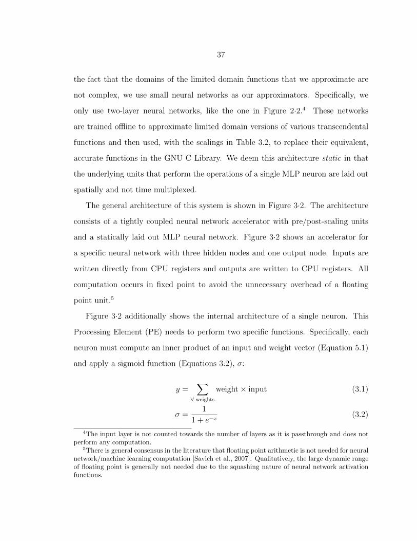
37
the fact that the domains of the limited domain functions that we approximate are
not complex, we use small neural networks as our approximators. Specifically, we
only use two-layer neural networks, like the one in Figure 2·2.4 These networks
are trained offline to approximate limited domain versions of various transcendental
functions and then used, with the scalings in Table 3.2, to replace their equivalent,
accurate functions in the GNU C Library. We deem this architecture static in that
the underlying units that perform the operations of a single MLP neuron are laid out
spatially and not time multiplexed.
The general architecture of this system is shown in Figure 3·2. The architecture
consists of a tightly coupled neural network accelerator with pre/post-scaling units
and a statically laid out MLP neural network. Figure 3·2 shows an accelerator for
a specific neural network with three hidden nodes and one output node. Inputs are
written directly from CPU registers and outputs are written to CPU registers. All
computation occurs in fixed point to avoid the unnecessary overhead of a floating
point unit.5
Figure 3·2 additionally shows the internal architecture of a single neuron. This
Processing Element (PE) needs to perform two specific functions. Specifically, each
neuron must compute an inner product of an input and weight vector (Equation 5.1)
and apply a sigmoid function (Equations 3.2), σ:
y =∑
∀ weights
weight× input (3.1)
σ =1
1 + e−x(3.2)
4The input layer is not counted towards the number of layers as it is passthrough and does notperform any computation.
5There is general consensus in the literature that floating point arithmetic is not needed for neuralnetwork/machine learning computation [Savich et al., 2007]. Qualitatively, the large dynamic rangeof floating point is generally not needed due to the squashing nature of neural network activationfunctions.
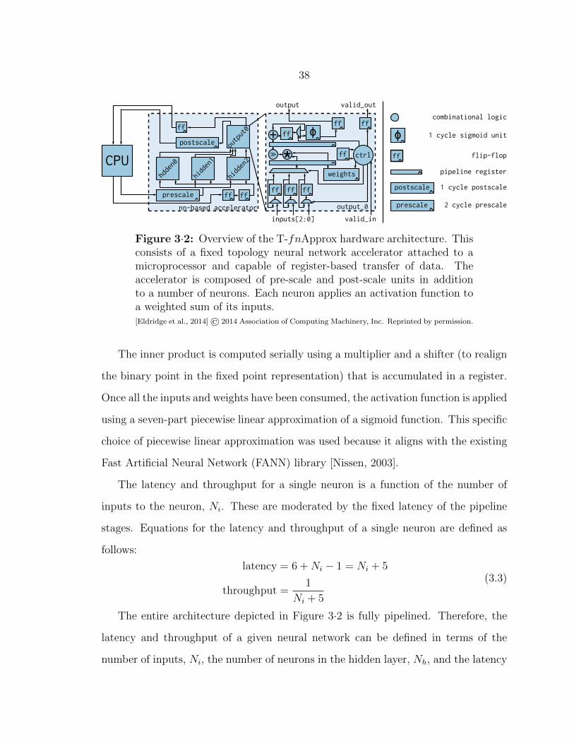
38
CPU
nn-based accelerator
hdden0
hidden1
hidden2
output0
ff ff ff
weights
ctrl*>>
+ ff ϕ
inputs[2:0] valid_in
valid_outoutput
output_0
ff
postscale
pipeline register
combinational logic
ϕ 1 cycle sigmoid unit
flip-flopff
ff
ffff
1 cycle postscalepostscale
2 cycle prescaleprescale
prescale ff
ff
Figure 3·2: Overview of the T-fnApprox hardware architecture. Thisconsists of a fixed topology neural network accelerator attached to amicroprocessor and capable of register-based transfer of data. Theaccelerator is composed of pre-scale and post-scale units in additionto a number of neurons. Each neuron applies an activation function toa weighted sum of its inputs.[Eldridge et al., 2014] © 2014 Association of Computing Machinery, Inc. Reprinted by permission.
The inner product is computed serially using a multiplier and a shifter (to realign
the binary point in the fixed point representation) that is accumulated in a register.
Once all the inputs and weights have been consumed, the activation function is applied
using a seven-part piecewise linear approximation of a sigmoid function. This specific
choice of piecewise linear approximation was used because it aligns with the existing
Fast Artificial Neural Network (FANN) library [Nissen, 2003].
The latency and throughput for a single neuron is a function of the number of
inputs to the neuron, Ni. These are moderated by the fixed latency of the pipeline
stages. Equations for the latency and throughput of a single neuron are defined as
follows:
latency = 6 +Ni − 1 = Ni + 5
throughput =1
Ni + 5
(3.3)
The entire architecture depicted in Figure 3·2 is fully pipelined. Therefore, the
latency and throughput of a given neural network can be defined in terms of the
number of inputs, Ni, the number of neurons in the hidden layer, Nh, and the latency
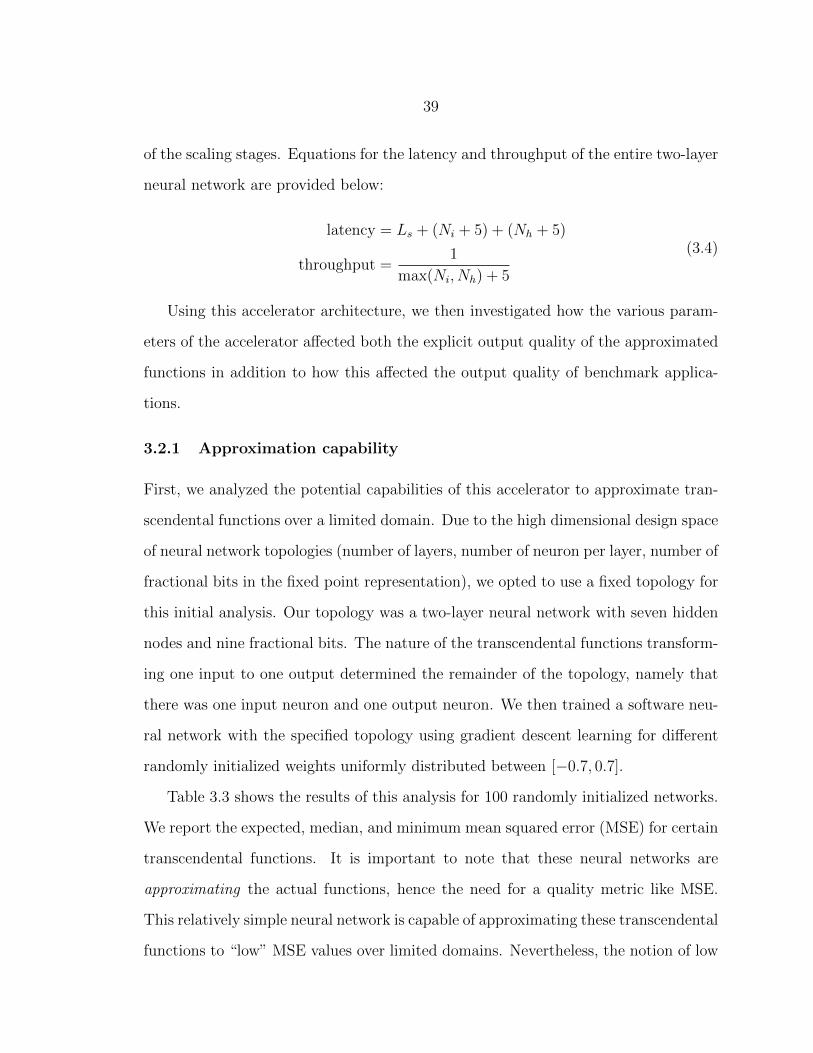
39
of the scaling stages. Equations for the latency and throughput of the entire two-layer
neural network are provided below:
latency = Ls + (Ni + 5) + (Nh + 5)
throughput =1
max(Ni, Nh) + 5
(3.4)
Using this accelerator architecture, we then investigated how the various param-
eters of the accelerator affected both the explicit output quality of the approximated
functions in addition to how this affected the output quality of benchmark applica-
tions.
3.2.1 Approximation capability
First, we analyzed the potential capabilities of this accelerator to approximate tran-
scendental functions over a limited domain. Due to the high dimensional design space
of neural network topologies (number of layers, number of neuron per layer, number of
fractional bits in the fixed point representation), we opted to use a fixed topology for
this initial analysis. Our topology was a two-layer neural network with seven hidden
nodes and nine fractional bits. The nature of the transcendental functions transform-
ing one input to one output determined the remainder of the topology, namely that
there was one input neuron and one output neuron. We then trained a software neu-
ral network with the specified topology using gradient descent learning for different
randomly initialized weights uniformly distributed between [−0.7, 0.7].
Table 3.3 shows the results of this analysis for 100 randomly initialized networks.
We report the expected, median, and minimum mean squared error (MSE) for certain
transcendental functions. It is important to note that these neural networks are
approximating the actual functions, hence the need for a quality metric like MSE.
This relatively simple neural network is capable of approximating these transcendental
functions to “low” MSE values over limited domains. Nevertheless, the notion of low
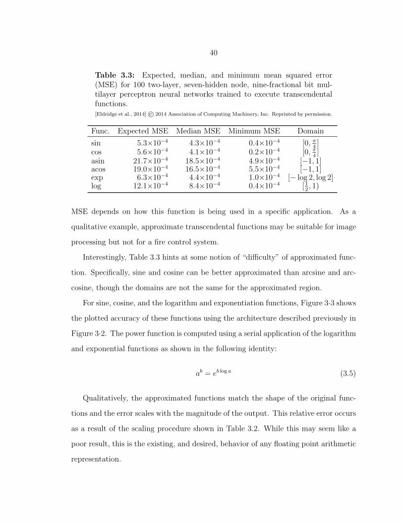
40
Table 3.3: Expected, median, and minimum mean squared error(MSE) for 100 two-layer, seven-hidden node, nine-fractional bit mul-tilayer perceptron neural networks trained to execute transcendentalfunctions.[Eldridge et al., 2014] © 2014 Association of Computing Machinery, Inc. Reprinted by permission.
Func. Expected MSE Median MSE Minimum MSE Domain
sin 5.3×10⁻⁴ 4.3×10⁻⁴ 0.4×10⁻⁴ [0, π4]
cos 5.6×10⁻⁴ 4.1×10⁻⁴ 0.2×10⁻⁴ [0, π4]
asin 21.7×10⁻⁴ 18.5×10⁻⁴ 4.9×10⁻⁴ [−1, 1]acos 19.0×10⁻⁴ 16.5×10⁻⁴ 5.5×10⁻⁴ [−1, 1]exp 6.3×10⁻⁴ 4.4×10⁻⁴ 1.0×10⁻⁴ [− log 2, log 2]log 12.1×10⁻⁴ 8.4×10⁻⁴ 0.4×10⁻⁴ [1
2, 1)
MSE depends on how this function is being used in a specific application. As a
qualitative example, approximate transcendental functions may be suitable for image
processing but not for a fire control system.
Interestingly, Table 3.3 hints at some notion of “difficulty” of approximated func-
tion. Specifically, sine and cosine can be better approximated than arcsine and arc-
cosine, though the domains are not the same for the approximated region.
For sine, cosine, and the logarithm and exponentiation functions, Figure 3·3 shows
the plotted accuracy of these functions using the architecture described previously in
Figure 3·2. The power function is computed using a serial application of the logarithm
and exponential functions as shown in the following identity:
ab = eb log a (3.5)
Qualitatively, the approximated functions match the shape of the original func-
tions and the error scales with the magnitude of the output. This relative error occurs
as a result of the scaling procedure shown in Table 3.2. While this may seem like a
poor result, this is the existing, and desired, behavior of any floating point arithmetic
representation.
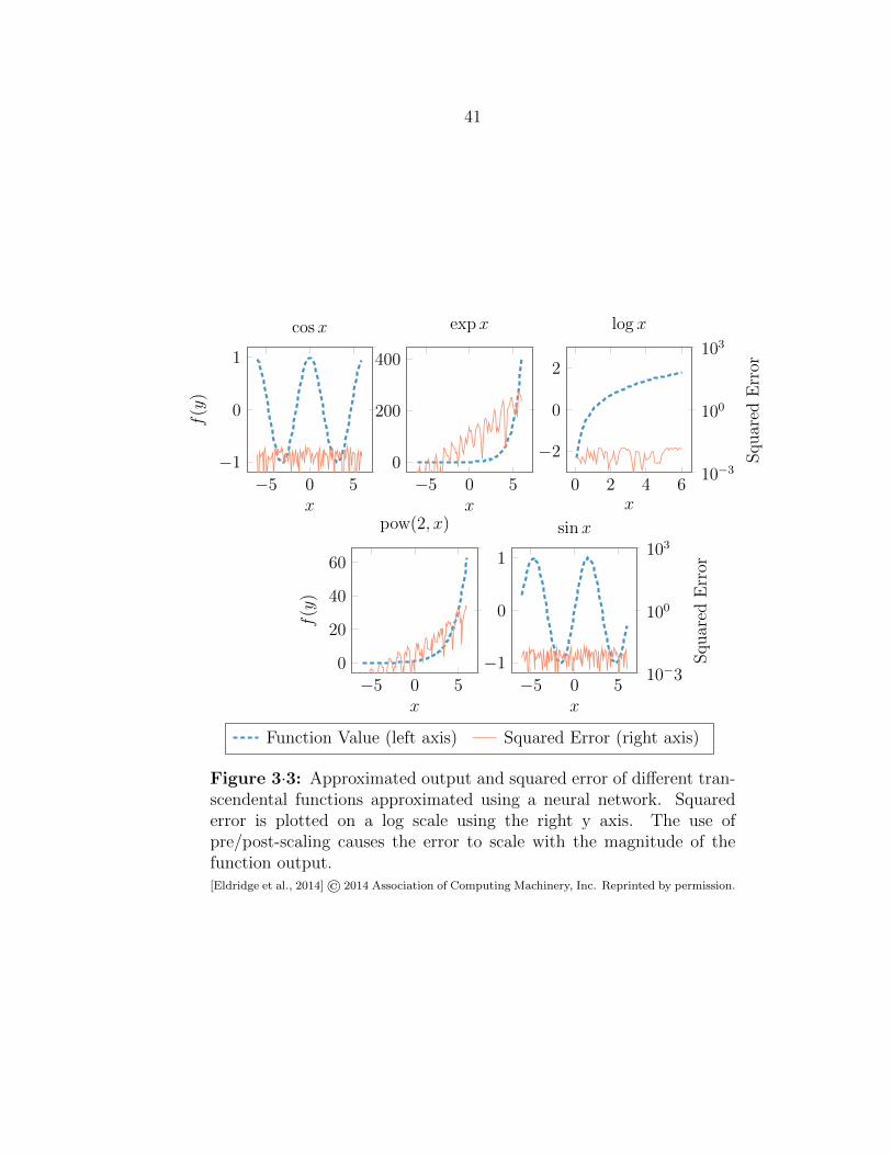
41
−5 0 5
−1
0
1
x
f(y
)
cosx
−5 0 5
0
200
400
x
expx
0 2 4 6
−2
0
2
x
log x
−5 0 5
0
20
40
60
x
f(y
)
pow(2, x)
−5 0 5
−1
0
1
x
sinx
10−3
100
103
Squar
edE
rror
10−3
100
103
Squar
edE
rror
Function Value (left axis) Squared Error (right axis)
Figure 3·3: Approximated output and squared error of different tran-scendental functions approximated using a neural network. Squarederror is plotted on a log scale using the right y axis. The use ofpre/post-scaling causes the error to scale with the magnitude of thefunction output.[Eldridge et al., 2014] © 2014 Association of Computing Machinery, Inc. Reprinted by permission.
42
3.3 Evaluation
We then evaluate a hardware implementation of the previously described neural net-
work accelerator architecture on grounds of energy and performance. Our primary
comparison point is against a traditional implementation using floating point arith-
metic and the GNU C Library.
3.3.1 Energy efficiency
With this work, we leverage the decrease in the accuracy of these transcendental
functions to increase the energy efficiency of applications. To do this, we pushed
a Verilog description of the neural network accelerator for different configurations
through a Cadence toolflow using the NCSU FreePDK 45nm predictive technology
model [Stine et al., 2007].
As our approximation trade off introduces an element of accuracy we define an
error metric that incorporates the MSE of a given configuration, energy delay error
product (EDEP):
EDEP = energy× latency in cycles
frequency×MSE (3.6)
The neural networks with minimum EDEP were found to have one hidden node
and six bits of fixed point precision. Exponential and logarithmic functions used
three hidden nodes and seven bits of fixed point precision. Table 3.4 shows the
area, maximum operating frequency, and energy per operation (one feedforward pass
through the neural network). Surprisingly, these networks are incredibly simple and
have extremely limited precision compared to traditional computation in a modern
computer architecture (32 or 64 bits for integer math and 24 or 53 for floating point).
As mentioned previously, two neural networks in series, one configured to perform
an exponential function and another configured to perform a logarithm, can be used

43
Table 3.4: Neural network accelerator hardware parameters with min-imum energy delay error product (EDEP) for sin, cos, log, and exp.Data is from a placed and routed design in a 45nm predictive technol-ogy model [Stine et al., 2007].[Eldridge et al., 2014] © 2014 Association of Computing Machinery, Inc. Reprinted by permission.
Function Topology Precision Area (um2) Freq. (MHz) Energy (pJ)
cos, sin 1× 1× 1 6-bit 1259.50 337.38 8.30exp, log 1× 3× 7 7-bit 3578.50 335.80 24.81
Table 3.5: Mean squared error (MSE) and energy consumption of ourneural network accelerated version of transcendental functions.[Eldridge et al., 2014] © 2014 Association of Computing Machinery, Inc. Reprinted by permission.
Function Topology MSE Energy (pJ)
cos 1× 1× 1 9.38×10⁻⁴ 8.30exp 1× 3× 7 1.68×10⁻⁴ 24.81log 1× 3× 7 1.45×10⁻⁴ 24.81pow 1× 3× 7 4.32×10⁻² 101.67sin 1× 1× 1 7.37×10⁻⁴ 8.30
to compute the power function via Equation 3.5. Table 3.5 shows the MSE and energy
per operation for all transcendental functions that we consider. The cost of the power
function is higher because this requires additional logic to be statically laid out and
drives up the overall energy.
3.3.2 Comparison against traditional floating point
Our primary comparison point for this work was against the traditional floating point
implementation of these transcendental functions used by the GNU C Library. We
computed the expected instruction counts for transcendental functions in the GNU
C Library using the gem5 system simulator [Binkert et al., 2011] to track executed
instructions. We used custom micro-benchmarks comprised of loops of transcendental
functions on random inputs. Instruction counts were averaged across all executions
of the loops.
Figure 3·4 shows the count of each floating point instruction used (additions, sub-
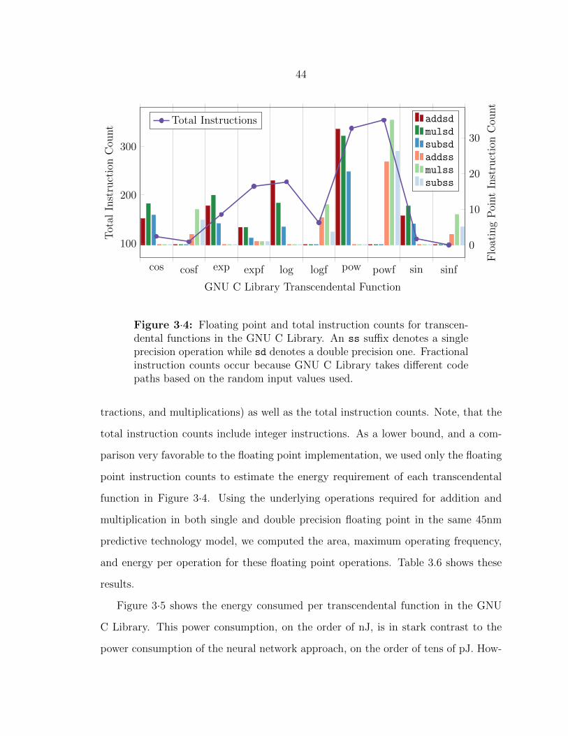
44
cos cosf exp expf log logf pow powf sin sinf
0
10
20
30
GNU C Library Transcendental Function
Flo
atin
gP
oint
Inst
ruct
ion
Cou
nt
addsdmulsdsubsdaddssmulsssubss
100
200
300
Tot
alIn
stru
ctio
nC
ount
Total Instructions
Figure 3·4: Floating point and total instruction counts for transcen-dental functions in the GNU C Library. An ss suffix denotes a singleprecision operation while sd denotes a double precision one. Fractionalinstruction counts occur because GNU C Library takes different codepaths based on the random input values used.
tractions, and multiplications) as well as the total instruction counts. Note, that the
total instruction counts include integer instructions. As a lower bound, and a com-
parison very favorable to the floating point implementation, we used only the floating
point instruction counts to estimate the energy requirement of each transcendental
function in Figure 3·4. Using the underlying operations required for addition and
multiplication in both single and double precision floating point in the same 45nm
predictive technology model, we computed the area, maximum operating frequency,
and energy per operation for these floating point operations. Table 3.6 shows these
results.
Figure 3·5 shows the energy consumed per transcendental function in the GNU
C Library. This power consumption, on the order of nJ, is in stark contrast to the
power consumption of the neural network approach, on the order of tens of pJ. How-
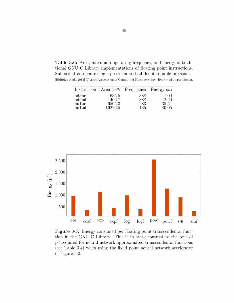
45
Table 3.6: Area, maximum operating frequency, and energy of tradi-tional GNU C Library implementations of floating point instructions.Suffixes of ss denote single precision and sd denote double precision.[Eldridge et al., 2014] © 2014 Association of Computing Machinery, Inc. Reprinted by permission.
Instruction Area (um2) Freq. (MHz) Energy (pJ)
addss 635.5 388 1.00addsd 1466.7 388 2.20mulss 6505.3 283 35.51mulsd 16226.5 135 80.05
cos cosf exp expf log logf pow powf sin sinf
500
1,000
1,500
2,000
2,500
Ener
gy(p
J)
Figure 3·5: Energy consumed per floating point transcendental func-tion in the GNU C Library. This is in stark contrast to the tens ofpJ required for neural network approximated transcendental functions(see Table 3.4) when using the fixed point neural network acceleratorof Figure 3·2.
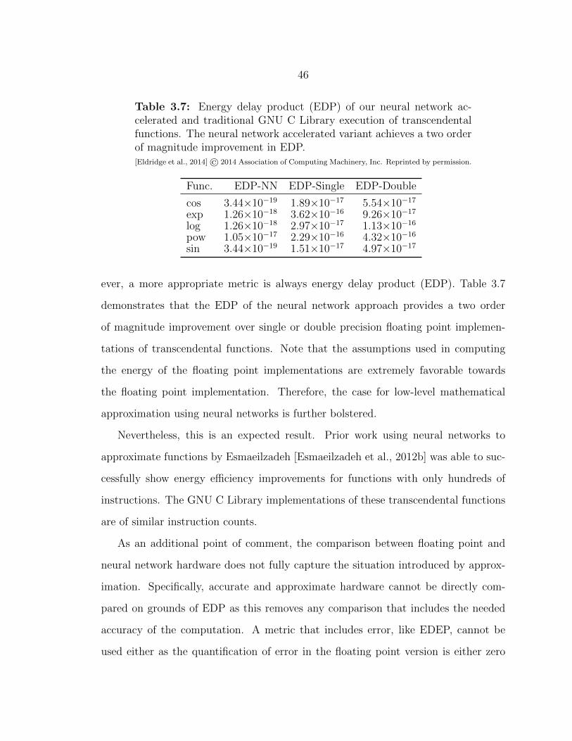
46
Table 3.7: Energy delay product (EDP) of our neural network ac-celerated and traditional GNU C Library execution of transcendentalfunctions. The neural network accelerated variant achieves a two orderof magnitude improvement in EDP.[Eldridge et al., 2014] © 2014 Association of Computing Machinery, Inc. Reprinted by permission.
Func. EDP-NN EDP-Single EDP-Double
cos 3.44×10⁻¹⁹ 1.89×10⁻¹⁷ 5.54×10⁻¹⁷
exp 1.26×10⁻¹⁸ 3.62×10⁻¹⁶ 9.26×10⁻¹⁷
log 1.26×10⁻¹⁸ 2.97×10⁻¹⁷ 1.13×10⁻¹⁶
pow 1.05×10⁻¹⁷ 2.29×10⁻¹⁶ 4.32×10⁻¹⁶
sin 3.44×10⁻¹⁹ 1.51×10⁻¹⁷ 4.97×10⁻¹⁷
ever, a more appropriate metric is always energy delay product (EDP). Table 3.7
demonstrates that the EDP of the neural network approach provides a two order
of magnitude improvement over single or double precision floating point implemen-
tations of transcendental functions. Note that the assumptions used in computing
the energy of the floating point implementations are extremely favorable towards
the floating point implementation. Therefore, the case for low-level mathematical
approximation using neural networks is further bolstered.
Nevertheless, this is an expected result. Prior work using neural networks to
approximate functions by Esmaeilzadeh [Esmaeilzadeh et al., 2012b] was able to suc-
cessfully show energy efficiency improvements for functions with only hundreds of
instructions. The GNU C Library implementations of these transcendental functions
are of similar instruction counts.
As an additional point of comment, the comparison between floating point and
neural network hardware does not fully capture the situation introduced by approx-
imation. Specifically, accurate and approximate hardware cannot be directly com-
pared on grounds of EDP as this removes any comparison that includes the needed
accuracy of the computation. A metric that includes error, like EDEP, cannot be
used either as the quantification of error in the floating point version is either zero
47
(if floating point is the baseline) or extremely small and likely biasing the results to
always favor floating point. A slight reconciliation can be provided with the following
explanation. Floating point, as previously stated, is an extremely blunt instrument
and generally not necessary—how many computations really need 24 or 53 bits of
precision? However, floating point (or 32/64 bit integers) are the only computational
formats available. What this, and other work in the approximate computing liter-
ature, demonstrates is that there exists extreme opportunities for energy efficiency
gains by using just enough computation necessary for a given function or application.
3.3.3 Affect on application benchmarks
To provide a more holistic viewpoint of the use of this neural network accelerator
as a mathematical function approximator, we approximate transcendental functions
in several benchmarks in the PARSEC benchmark suite [Bienia, 2011] and evaluate
the overall loss in application output quality. Initially, we determined the number of
cycles that each PARSEC benchmark spent computing the transcendental functions
which we approximate. In an Amdahl’s Law-like argument, any gain that we see will
be a function of what percentage of the time a given application spends computing
transcendental functions. Table 3.8 shows the percentage of cycles as well as the
resulting normalized EDP from using our neural network accelerator.
Five of the applications we tested used floating point functions.6 Two of them,
blackscholes and swaptions, spent a significant amount of time on transcenden-
tal functions. This resulted in normalized EDP improvements of nearly 50%. For
bodytrack and canneal transcendental functions did not constitute a dominant por-
tion of their runtimes. Other applications evaluated did not use floating point tran-
scendental functions which resulted in no change in the EDP of these applications.7
6For ferret we were unable to get cycle counts using gem5.7Any contribution of our neural network accelerator towards power consumption is negligible
compared to the rest of the microprocessor.

48
Table 3.8: Percentage of total application cycles spent in transcenden-tal functions and the estimated energy delay product (EDP) of usingour neural network accelerator to approximate these functions. EDPresults are normalized against single precision floating point implemen-tations. Applications in the lower division have no transcendental func-tions and see no change in EDP. Applications are taken from the PAR-SEC benchmark suite [Bienia, 2011].[Eldridge et al., 2014] © 2014 Association of Computing Machinery, Inc. Reprinted by permission.
Benchmark % Total Cycles Normalized EDP
blackscholes 45.65% 0.5583bodytrack 2.25% 0.9783canneal 1.19% 0.9885swaptions 39.33% 0.6191
dedup 0.00% 1.0000fluidanimate 0.00% 1.0000freqmine 0.00% 1.0000raytrace 0.00% 1.0000streamcluster 0.00% 1.0000x264 0.00% 1.0000vips 0.00% 1.0000
The resulting loss in application output quality was also measured. Table 3.9
shows the expected percentage error between the generated output and the expected
output for the application. The use of neural networks to approximate transcendental
functions did not result in any application failures.
3.4 Approximation and Fixed-topology Neural Network Ac-
celerators
It is important to note that our specific choice of floating point mathematical instruc-
tions for approximation was not arbitrary. We were originally tempted to approx-
imated integer operations. However, this introduces problems in that the safety of
an approximation depends on how an integer value is used. For example, an integer
value that represents a pixel is a suitable approximation target, however an address
computation is not.
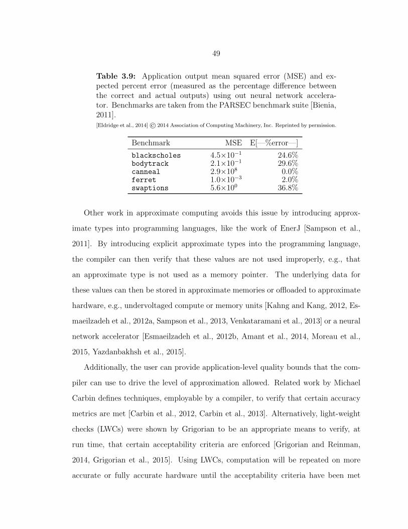
49
Table 3.9: Application output mean squared error (MSE) and ex-pected percent error (measured as the percentage difference betweenthe correct and actual outputs) using out neural network accelera-tor. Benchmarks are taken from the PARSEC benchmark suite [Bienia,2011].[Eldridge et al., 2014] © 2014 Association of Computing Machinery, Inc. Reprinted by permission.
Benchmark MSE E[—%error—]
blackscholes 4.5×10⁻¹ 24.6%bodytrack 2.1×10⁻¹ 29.6%canneal 2.9×10⁸ 0.0%ferret 1.0×10⁻³ 2.0%swaptions 5.6×100 36.8%
Other work in approximate computing avoids this issue by introducing approx-
imate types into programming languages, like the work of EnerJ [Sampson et al.,
2011]. By introducing explicit approximate types into the programming language,
the compiler can then verify that these values are not used improperly, e.g., that
an approximate type is not used as a memory pointer. The underlying data for
these values can then be stored in approximate memories or offloaded to approximate
hardware, e.g., undervoltaged compute or memory units [Kahng and Kang, 2012, Es-
maeilzadeh et al., 2012a, Sampson et al., 2013, Venkataramani et al., 2013] or a neural
network accelerator [Esmaeilzadeh et al., 2012b, Amant et al., 2014, Moreau et al.,
2015, Yazdanbakhsh et al., 2015].
Additionally, the user can provide application-level quality bounds that the com-
piler can use to drive the level of approximation allowed. Related work by Michael
Carbin defines techniques, employable by a compiler, to verify that certain accuracy
metrics are met [Carbin et al., 2012, Carbin et al., 2013]. Alternatively, light-weight
checks (LWCs) were shown by Grigorian to be an appropriate means to verify, at
run time, that certain acceptability criteria are enforced [Grigorian and Reinman,
2014, Grigorian et al., 2015]. Using LWCs, computation will be repeated on more
accurate or fully accurate hardware until the acceptability criteria have been met
50
or surpassed. As an alternative to hardware-based approaches, software-only tech-
niques, like loop-perforation or early termination, can be exploited to use approximate
computing techniques without hardware modifications [Rinard, 2007, Agarwal et al.,
2009, Sidiroglou-Douskos et al., 2011].
Nevertheless, an open question is, broadly, what applications can be safely ap-
proximated. Intuitively, and following the discussion of floating point as a blunt
instrument, computation should only use as much precision as needed. However, the
constraints of hardware being fixed and the quantized nature of underlying arithmetic
types forces software developers to use much more precision than is often needed, as
has been deftly identified by Venkataramani [Venkataramani et al., 2013]. It is no
wonder that benchmark applications have been demonstrated, experimentally, by
Chen [Chen et al., 2012] and Chippa [Chippa et al., 2013] to be amenable to approx-
imation techniques, using neural network accelerator hardware or otherwise.
With the work presented in this chapter, T-fnApprox, we demonstrate that less
stringent checks can be advantageous in that they dramatically reduce the EDP of
individual computations without adversely affecting the output quality of computa-
tions. While not specifically evaluated, a more heavily optimized implementation of
mathematical functions, e.g., one provided by Automatically Tuned Linear Algebra
Software (ATLAS) or Basic Linear Algebra Subprograms (BLAS), would have less
margin for improvement compared with the GNU C Library.
However, the approximate nature of this work was only one component. We also
proposed an initial version of a neural network accelerator architecture. In the taxon-
omy provided by Grigorian [Grigorian et al., 2015], T-fnApprox is a fixed connection,
fixed weight/bias accelerator.8 The fixed nature of T-fnApprox, while resulting in
the largest possible EDP gains, is not suited for general purpose neural network ac-
celeration, i.e., class SNN of our ontology. This is due to the diverse and unknown
8This is what we have referred to previously as a fixed topology accelerator.
51
nature of neural network topologies used by applications. To work for a different neu-
ral network topology, T-fnApprox requires the use of a different, statically structured
architecture for each different neural network that a user wants to use—in effect, a
new accelerator for each network. Alternatively, a large fixed connection, variable
weight/bias accelerator, is also tenable, but inefficient as PEs are underutilized.
In conclusion, while a fixed topology accelerator provides the highest possible
energy efficiency improvements for approximate computing applications, the most
general system is one that allows for variable connections and variable weights/biases.
As a result of this, followup work discussed in subsequent chapters introduces a generic
neural network accelerator architecture capable of running arbitrary neural networks
for approximate computing or other applications.

52
Chapter 4
X-FILES: Software/Hardware for Neural
Networks as First Class Primitives
Following work on T-fnApprox and motivated by work related to automatic par-
allelization [Waterland et al., 2012, Waterland et al., 2014], we developed a neural
network accelerator architecture composed of dynamically allocated PEs. This ar-
chitecture, a Dynamically Allocated Neural Network Accelerator or DANA, forms
the computational backend of a microprocessor/coprocessor system for the purposes
of accelerating neural network computation. However, the use of DANA, or any
neural network accelerator for that matter, directly interfaced with a microproces-
sor necessitates both the software/hardware intricacies of accelerator design and our
aforementioned goals of a multi-context accelerator for the ubiquitous use of machine
learning. In consequence, we diverge initially and provide a discussion of our set of
software/hardware Extensions for the Integration of Machine Learning in Everyday
Systems or X-FILES. The X-FILES extensions treat neural network computation as
a fundamental primitive of applications, like floating point computation. We defer
an exhaustive discussion of DANA until Chapter 5 in light of the fact that concepts
necessary to understand DANA are introduced in this chapter.
4.1 Motivation: Neural Networks as Function Primitives
As outlined previously, we are motivated by the increasing interest in machine learn-
ing as evidenced by emerging applications in approximate computing and automatic

53
parallelization. In these applications, machine learning is not the underlying applica-
tion, but a component of the application. While we acknowledge the subtlety of this
differentiation, said differentiation is governed by the degree of adoption of machine
learning as a computational kernel and, hence, drives the need for dedicated software
and hardware like the X-FILES extensions and DANA.
This difference can be briefly stated with an example. Machine learning is typ-
ically used for an application domain like the image labeling task of the ImageNet
dataset [Deng et al., 2009]. Image labeling, and machine learning generally, devolves
into a problem of learning and inference—a dataset is provided, a model is trained,
and that model is applied to new, unseen data. A general model of learning and
inference matches the requirements of existing components of hardware and software,
e.g., branch prediction by a microprocessor, cache prefetching by an operating sys-
tem, and malware detection by antivirus software. Here, machine learning is not the
application, but a formalized approach to learning and inference competing with a
developer-specified heuristic.
In clarification, when we state that our goal is to make hardware-accelerated
machine learning or neural network computation a general component or first class
primitive of applications we mean, broadly, exposing hardware acceleration of the pre-
eminent learning/inference technique available as a general resource to applications.
We then posit that our multi-transaction model meets the needs of these future ap-
plications and we seek to develop infrastructure, the X-FILES extensions, in support
of this model.
Figure 4·1 shows a high-level overview of a multiprocessing system. This system is
composed of N processes whose access to the underlying hardware is moderated by an
operating system (OS). Assuming that this is a virtual memory system, each process
thinks that it has complete access to all available memory and, thereby, lives in its
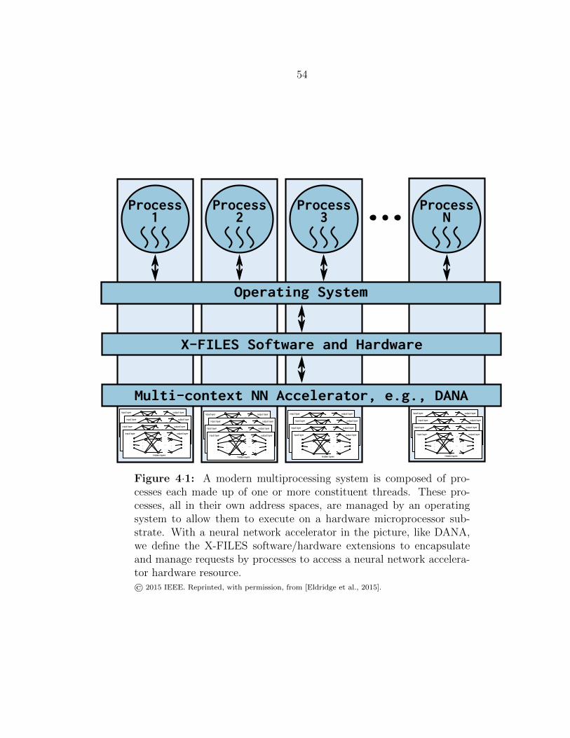
54
Operating System
X-FILES Software and Hardware
Multi-context NN Accelerator, e.g., DANA
Process2
Process1
Process3
ProcessN
input layer output layer
hidden layers
...
......
.
.
.
.
.
.
input layer output layer
hidden layers
...
......
.
.
.
.
.
.
input layer output layer
hidden layers
...
......
.
.
.
.
.
.
input layer output layer
hidden layers
...
......
.
.
.
.
.
.
input layer output layer
hidden layers
...
......
.
.
.
.
.
.
input layer output layer
hidden layers
...
......
.
.
.
.
.
.
input layer output layer
hidden layers
...
......
.
.
.
.
.
.
input layer output layer
hidden layers
...
......
.
.
.
.
.
.
input layer output layer
hidden layers
...
......
.
.
.
.
.
.
input layer output layer
hidden layers
...
......
.
.
.
.
.
.
input layer output layer
hidden layers
...
......
.
.
.
.
.
.
input layer output layer
hidden layers
...
......
.
.
.
.
.
.
input layer output layer
hidden layers
...
......
.
.
.
.
.
.
input layer output layer
hidden layers
...
......
.
.
.
.
.
.
input layer output layer
hidden layers
...
......
.
.
.
.
.
.
input layer output layer
hidden layers
...
......
.
.
.
.
.
.
Figure 4·1: A modern multiprocessing system is composed of pro-cesses each made up of one or more constituent threads. These pro-cesses, all in their own address spaces, are managed by an operatingsystem to allow them to execute on a hardware microprocessor sub-strate. With a neural network accelerator in the picture, like DANA,we define the X-FILES software/hardware extensions to encapsulateand manage requests by processes to access a neural network accelera-tor hardware resource.© 2015 IEEE. Reprinted, with permission, from [Eldridge et al., 2015].
55
own address space. Each address space can be identified with its own address space
identifier or ASID indicated by the vertical boxes separating one process from another.
Each process, wants to access specific neural networks, indicated by the graphical
networks in each process’ address space. In a traditional coprocessor implementation
(e.g., a floating point unit), each process is given exclusive access to the underlying
hardware resources. However, neural network computation is markedly different from
the types of computation traditional coprocessors execute.
First, we digress and comment on a unit of coprocessor work. We define a unit
of work for a coprocessor (or neural network accelerator going forward) as a trans-
action. A transaction encapsulates the request by a user process to do some work
(e.g., a neural network transaction could be, verbally, “Compute the output of neural
network X for input vector Y and put the result in Z.”). An inference transaction
thereby includes the following components:
• A user-specified identifier indicating which neural network to use, i.e., a neural
network identifier or NNID
• A user-specified input vector to the network
• An accelerator-generated output vector
A learning transaction includes all the components of an inference transaction, but
also includes an expected output vector for each input vector and has an associated
parameter indicating the batch size of the learning operation.1 The accelerator and
the user agree on a unique way of talking about the specific transaction, i.e., the
transaction has an associated transaction identifier or TID. Note that the amount
of work encapsulated by a transaction depends on a number of parameters of the
1The batch size is the number of input–expected output vectors that will be used before updatingthe weights of the neural network. A batch size of one is stochastic gradient descent—the networkis updated from the computed gradient of a single sample—while a batch size equal to the size ofthe training set is gradient descent—the network is updated from the average gradient of the entiretraining set.
56
transaction:
• The specific neural network, i.e., the NNID
• The type of request, e.g., inference or learning
• The parameters of the request, e.g., the batch size of a learning request
To draw a contrast, consider the equivalent of a transaction in a floating point
coprocessor—an action encapsulating a request to perform a function with one or
more floating point numbers, e.g., “Multiply A by B and put the product in C.” Such
transactions, e.g., addition or multiplication, have negligible differences in their run-
times (on the order of cycles). However, the runtimes for neural network transactions
can be dramatically different, e.g., consider the difference in runtimes of a network
with millions of neurons versus a network with tens of neurons. This dramatic varia-
tion needs to be incorporated into the design of the accelerator and its management
infrastructure. Specifically, the runtime of a transaction could outlive the context of
a given process (tens of thousands of cycles). In order to better guarantee forward
progress, the transactions should operate independently of their associated processes.
Therefore, the underlying backend needs to be multi-context.
Multi-context accelerators are intrinsically complicated because they must guar-
antee the security of the data of all simultaneously executing contexts. However, this
complex problem can be succinctly described as transaction management or the man-
agement of ASIDs, NNIDs, and TIDs. More verbosely, the job of X-FILES hardware
and software is to manage transactions (identified with TIDs) requesting access to
specific neural networks (identified with NNIDs) for multiple processes in the same or
disparate address spaces (identified with ASIDs).
57
4.2 X-FILES: Software and Hardware for Transaction Man-
agement
With Figure 4·1 in mind, the X-FILES act as an intermediary between user processes
and the operating system and the underlying hardware. In effect, the X-FILES en-
compass all modifications to a system necessary to enable and use a multi-context
backend, like DANA. In an alternative formulation, the X-FILES hardware and soft-
ware extensions enable simultaneous multithreading (SMT) of neural network trans-
actions or virtualization of an accelerator backend. Due to the hardware/software
nature of these extensions, it is useful to build from a concrete description of an
interface between a microprocessor and an accelerator.
In the past, accelerators were traditionally relegated to a bus external to the
microprocessor, like PCIe. This is a sound design decision for devices that operate on
data independently of the microprocessor or act as specialized input–output hardware,
e.g., GPUs or high bandwidth Ethernet cards. However, there is a recent general
trend towards tighter integration of accelerators with microprocessors as accelerators
begin to augment and replace work which was traditionally done by a microprocessor
datapath. Additionally, this tight accelerator integration means that the accelerator
is potentially operating on the same data of the microprocessor or data which the
microprocessor is generating or consuming. This motivates the need for participation
by the accelerator in the cache coherency protocol.
These two motivations have led to new accelerator interfaces that meet these
needs, e.g., IBM currently provides the Coherent Accelerator Processor Interface
(CAPI). Similarly, UC Berkeley provides a Rocket Custom Coprocessor (RoCC) in-
terface for their RISC-V line of open source microprocessors. We standardize on the
RoCC interface, though any interface that provides the same features (e.g., CAPI)
can be considered functionally equivalent.
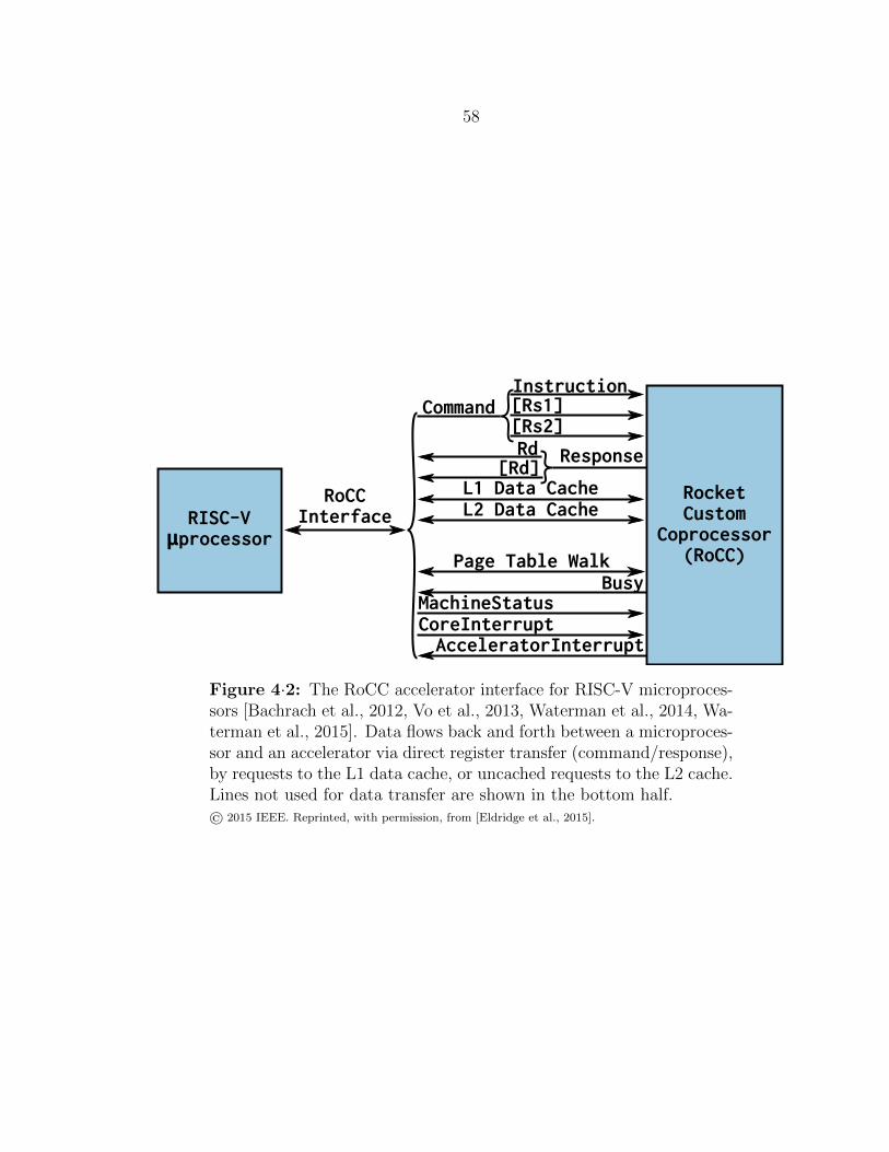
58
RocketCustom
Coprocessor(RoCC)
RISC-Vμprocessor
CommandInstruction[Rs1][Rs2]Rd Response
[Rd]
BusyMachineStatusCoreInterruptAcceleratorInterrupt
RoCCInterface
L1 Data Cache
Page Table Walk
L2 Data Cache
Figure 4·2: The RoCC accelerator interface for RISC-V microproces-sors [Bachrach et al., 2012, Vo et al., 2013, Waterman et al., 2014, Wa-terman et al., 2015]. Data flows back and forth between a microproces-sor and an accelerator via direct register transfer (command/response),by requests to the L1 data cache, or uncached requests to the L2 cache.Lines not used for data transfer are shown in the bottom half.© 2015 IEEE. Reprinted, with permission, from [Eldridge et al., 2015].
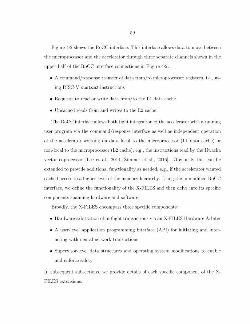
59
Figure 4·2 shows the RoCC interface. This interface allows data to move between
the microprocessor and the accelerator through three separate channels shown in the
upper half of the RoCC interface connections in Figure 4·2:
• A command/response transfer of data from/to microprocessor registers, i.e., us-
ing RISC-V customX instructions
• Requests to read or write data from/to the L1 data cache
• Uncached reads from and writes to the L2 cache
The RoCC interface allows both tight integration of the accelerator with a running
user program via the command/response interface as well as independent operation
of the accelerator working on data local to the microprocessor (L1 data cache) or
non-local to the microprocessor (L2 cache), e.g., the instructions read by the Hwacha
vector coprocessor [Lee et al., 2014, Zimmer et al., 2016]. Obviously this can be
extended to provide additional functionality as needed, e.g., if the accelerator wanted
cached access to a higher level of the memory hierarchy. Using the unmodified RoCC
interface, we define the functionality of the X-FILES and then delve into its specific
components spanning hardware and software.
Broadly, the X-FILES encompass three specific components:
• Hardware arbitration of in-flight transactions via an X-FILES Hardware Arbiter
• A user-level application programming interface (API) for initiating and inter-
acting with neural network transactions
• Supervisor-level data structures and operating system modifications to enable
and enforce safety
In subsequent subsections, we provide details of each specific component of the X-
FILES extensions.
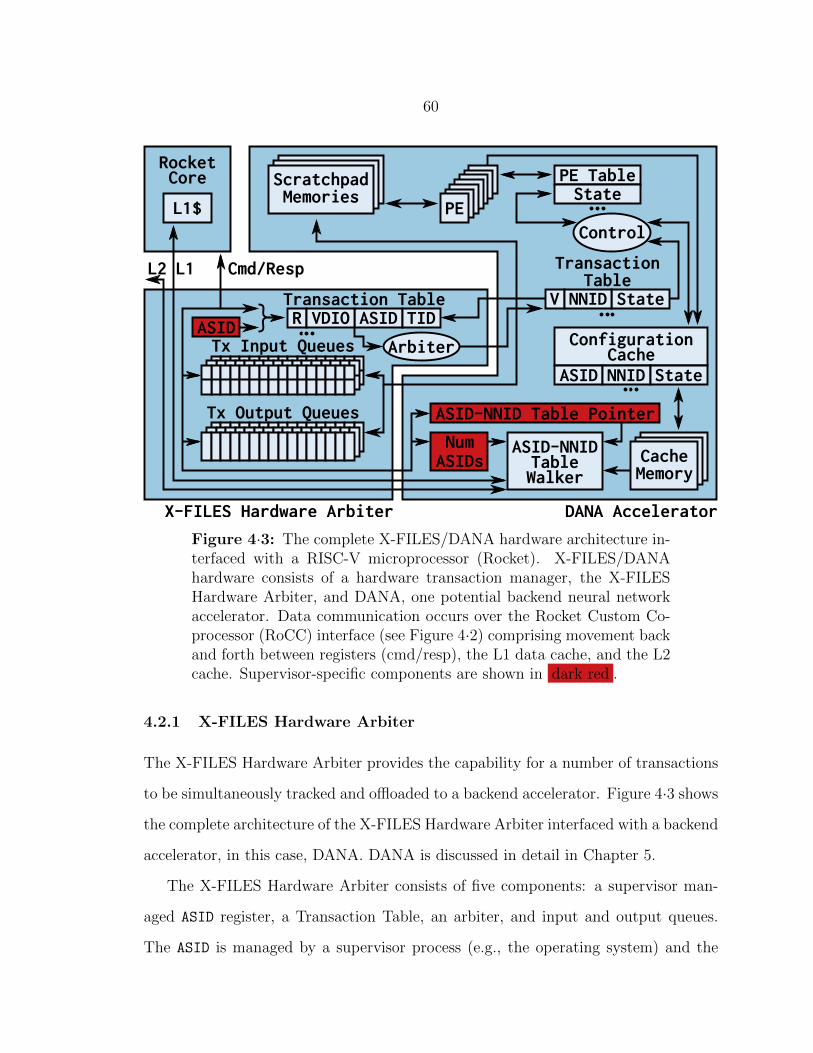
60
DANA AcceleratorX-FILES Hardware Arbiter
RocketCore
L1$
ASID
ASID-NNIDTableWalker
Arbiter
Control
PE
ConfigurationCache
ASID NNID State
CacheMemory
ScratchpadMemories
PE TableState
ASID-NNID Table Pointer
NumASIDs
Transaction TableASID TIDR VDIO
TransactionTable
StateV NNID
Cmd/RespL1L2
Tx Input Queues
Tx Output Queues
Figure 4·3: The complete X-FILES/DANA hardware architecture in-terfaced with a RISC-V microprocessor (Rocket). X-FILES/DANAhardware consists of a hardware transaction manager, the X-FILESHardware Arbiter, and DANA, one potential backend neural networkaccelerator. Data communication occurs over the Rocket Custom Co-processor (RoCC) interface (see Figure 4·2) comprising movement backand forth between registers (cmd/resp), the L1 data cache, and the L2cache. Supervisor-specific components are shown in dark red .
4.2.1 X-FILES Hardware Arbiter
The X-FILES Hardware Arbiter provides the capability for a number of transactions
to be simultaneously tracked and offloaded to a backend accelerator. Figure 4·3 shows
the complete architecture of the X-FILES Hardware Arbiter interfaced with a backend
accelerator, in this case, DANA. DANA is discussed in detail in Chapter 5.
The X-FILES Hardware Arbiter consists of five components: a supervisor man-
aged ASID register, a Transaction Table, an arbiter, and input and output queues.
The ASID is managed by a supervisor process (e.g., the operating system) and the
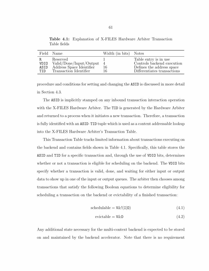
61
Table 4.1: Explanation of X-FILES Hardware Arbiter TransactionTable fields
Field Name Width (in bits) Notes
R Reserved 1 Table entry is in useVDIO Valid/Done/Input/Output 4 Controls backend executionASID Address Space Identifier 16 Defines the address spaceTID Transaction Identifier 16 Differentiates transactions
procedure and conditions for setting and changing the ASID is discussed in more detail
in Section 4.3.
The ASID is implicitly stamped on any inbound transaction interaction operation
with the X-FILES Hardware Arbiter. The TID is generated by the Hardware Arbiter
and returned to a process when it initiates a new transaction. Therefore, a transaction
is fully identified with an ASID–TID tuple which is used as a content addressable lookup
into the X-FILES Hardware Arbiter’s Transaction Table.
This Transaction Table tracks limited information about transactions executing on
the backend and contains fields shown in Table 4.1. Specifically, this table stores the
ASID and TID for a specific transaction and, through the use of VDIO bits, determines
whether or not a transaction is eligible for scheduling on the backend. The VDIO bits
specify whether a transaction is valid, done, and waiting for either input or output
data to show up in one of the input or output queues. The arbiter then chooses among
transactions that satisfy the following Boolean equations to determine eligibility for
scheduling a transaction on the backend or evictability of a finished transaction:
schedulable = V&!(I|O) (4.1)
evictable = V&D (4.2)
Any additional state necessary for the multi-context backend is expected to be stored
on and maintained by the backend accelerator. Note that there is no requirement
62
that the X-FILES backend be multi-context—the backend may be single-context or
even stateless combinational logic.
Data communication between the microprocessor and the X-FILES Hardware Ar-
biter can use any of the aforementioned command/response, cached L1, or uncached
L2 interfaces available to a backend. However, command/response register data goes
through the input/output queues. Using the user-level API, discussed in Section 4.2.3,
data is moved from microprocessor registers and entered in the input/output queues
with possible side effects to the X-FILES Transaction Table. The I and O bits of the
VDIO Transaction Table field will assert whenever the input queue is empty or the
output queue is full. By Equation 4.1, a stalled transaction waiting for input data or
space to put output data will be descheduled from the backend and rescheduled when
the stalling condition is cleared. The VDIO bits are asserted by the backend when re-
sponding to the X-FILES Hardware Arbiter following a transaction being scheduled.
Similarly, the VDIO bits are cleared by the X-FILES Hardware Arbiter, e.g., receipt
of input data clears the I bit.
Arbitration between schedulable transactions occurs in a round robin fashion.
However, we have considered (but not investigated) work-aware scheduling algorithms
to enforce some measure of fairness on backend transaction scheduling. Specifically,
the amount of work (effectively the size of the neural network requested by a transac-
tion) may be used to enforce fairness. As an example, a smaller neural network could
receive higher priority over a larger neural network. Similarly, priority could match
the niceness of the requesting process to provide lower latency to more time critical
transactions, e.g., those initiated by the operating system. This is discussed further
in Section 7.3.2.
All components of the X-FILES Hardware Arbiter were written in the Chisel
HDL [Bachrach et al., 2012] (a functional and object oriented HDL using Scala)

63
and are open sourced and available under a BSD License. This can be accessed on
GitHub [Boston University Integrated Circuits and Systems Group, 2016].
4.2.2 Supervisor data structures: the ASID–NNID Table
In terms of X-FILES software, this encompasses both modifications to supervisor soft-
ware, i.e., the operating system, as well as provisions for a user API for transactions.
The latter is discussed in the subsequent subsection. Here, we focus on modifications
to the operating system to provide safe, multi-context use of the backend accelerator.
We discuss some DANA-specific components, namely the NNID, but we attempt to
make references to how these data structures can be extended in a generic way.
The primary concern of a multi-context accelerator can be demonstrated by exam-
ining what happens on a context switch with a traditional floating point unit (FPU).
An FPU is, generally, an accelerator/coprocessor in the same context as a process
executing on the microprocessor. However, unlike straight combinational logic, e.g.,
the arithmetic logic unit (ALU), an FPU has some state, primarily, all of its floating
point registers. On a context switch, all these registers need to be saved alongside
the state of the process, i.e., inside the task struct (task struct in Linux), assuming
that the process has actually used the FPU.2 Relatedly, the registers also need to be
cleared before the new context is loaded. Otherwise, the FPU allows information to
leak from one process to another.
However, if the computations of the backend accelerator are long running, then a
multi-context accelerator makes sense assuming that the accelerator gets some benefit
from exposure to simultaneous, multi-context work. Unfortunately, this results in
2The RISC-V privileged specification has a description of how this is handled for the FPU andgeneric extensions (accelerators sitting in the RoCC socket) in Section 3.1.8 [Waterman et al., 2015].RISC-V uses a 2-bit value in the machine status (MSTATUS) register to indicate the state of theFPU (FS bits) or extension (XS bits) allowing for one of the following states: Off (disabled), Initial,Clean (matching the previously saved task struct), Dirty (differing from the previously savedtask struct).

64
significant additional complexity because one transaction must not be allowed to
access any information of another transaction. On the X-FILES Hardware Arbiter,
input and output data are segregated into per-transaction input and output queues.
However, this transfer of input and output data via the register interface only covers
one of the three ways that data can be communicated between the microprocessor
and the X-FILES. The others involve reads and writes via direct interfaces to the L1
and L2 caches. Put simply, the accelerator may elect to participate actively in the
cache coherency protocol.
This direct cache interface enables the backend accelerator to read or write large
amounts of information directly from or to memory. However, we must then consider
whether or not this data is provided as virtual or physical addresses. The former
depends on the context of the microprocessor being aligned with the ASID for that
data load (assuming that we’re not using a trivial operating system or bare metal
operation). Physical addresses are not, generally, available to the user process. Fur-
thermore, and much more importantly, the accelerator cannot blindly trust a physical
address given to it by a user process. The user process could be malicious and exploit
existing memory protection by using the accelerator to read regions of memory (e.g.,
cryptographic private keys) that it is not supposed to access.
To remedy this, we introduce an X-FILES supervisor data structure called an
ASID–NNID Table.3 The ASID–NNID Table, similar to a page table, provides a means
of dereferencing the location in memory of a specific neural network configuration
given an ASID and NNID.
Figure 4·4 shows an ASID–NNID Table. This table is anchored in the microproces-
sor’s memory with a base ASID–NNID Table Pointer (ANTP) which is provided to the
DANA backend by the operating system. In addition to the ANTP, the supervisor also
3Note that NNIDs are specific to DANA. However, the concept of some agreed upon identifier thatthe backend can use to find a specific program or data that it needs to move forward on some giventransaction is sound. Hence, the ASID–NNID Table can be viewed generally as an ASID–data table.

65
*NN Configuration
*NN Configuration
*NN Configuration
Header
Neurons
Weights
ASID-NNID Table Ptr*ASID-NNID *IO QueueNum NNIDs
*ASID-NNID *IO QueueNum NNIDs
*ASID-NNID *IO QueueNum NNIDs
Status/Header *Input *Output
Ring Buffers
Num ASIDs
Figure 4·4: An ASID–NNID Table that allows DANA to dereferencea given neural network configuration, identified with a neural networkidentifier (NNID), for a given process which has an assigned addressspace identifier (ASID). Both ASIDs and NNIDs are assigned sequentiallyto allow reuse of the ASID and NNID as table indices. Additionally, eachASID in the ASID–NNID Table has an in-memory input–output queue toallow for asynchronous transaction initiation and data transfer.© 2015 IEEE. Reprinted, with permission, from [Eldridge et al., 2015].
provides the number of valid ASIDs to prevent the hardware from reading memory be-
yond the last valid ASID. These fields can be seen in the overview of X-FILES/DANA
in Figure 4·3 and in Figure 4·4. For hardware convenience, both ASIDs and NNIDs are
assigned sequentially. This allows the ASID and NNID to be used as indices into the
ANTP.
A walk of the ASID–NNID Table can then be used to dereference a pointer to
some ASID-segregated data and indexed with an NNID by the backend accelerator. To
prevent additional memory exploits, each NNID table (the portion of the table indexed
using the NNID) has a known bound—the number of NNIDs (Num NNIDs in Figure 4·4).
All exceptional cases, which generate interrupts to the RISC-V microprocessor
are shown in Table 4.2. Note that only one of these, int INVREQ is specific to the
X-FILES Hardware Arbiter. The rest are all generated due to invalid operations
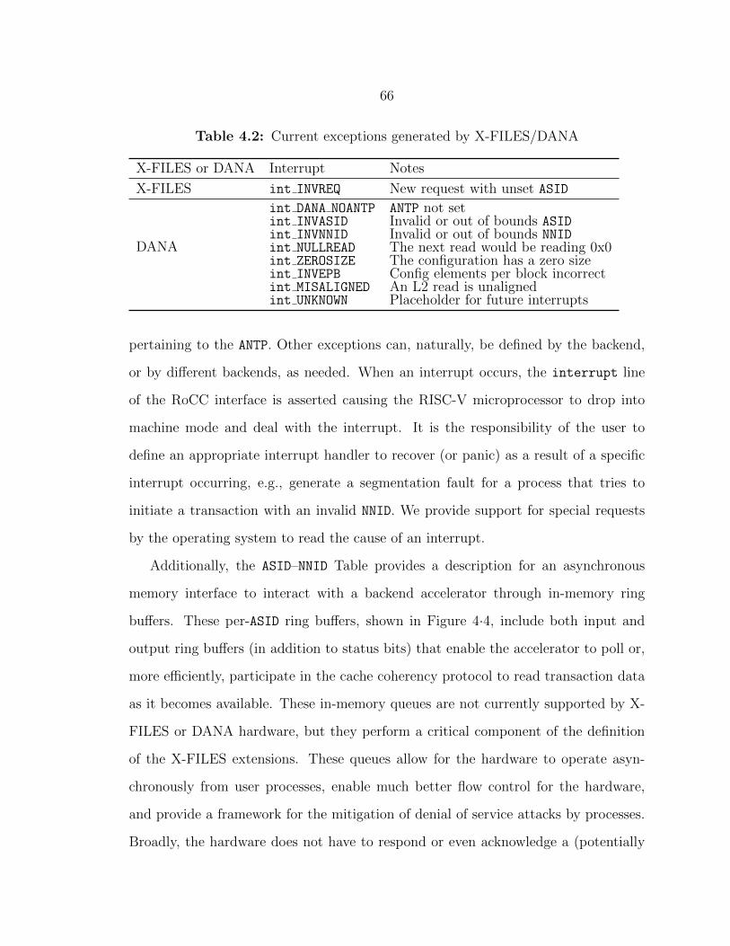
66
Table 4.2: Current exceptions generated by X-FILES/DANA
X-FILES or DANA Interrupt Notes
X-FILES int INVREQ New request with unset ASID
DANA
int DANA NOANTP ANTP not setint INVASID Invalid or out of bounds ASIDint INVNNID Invalid or out of bounds NNIDint NULLREAD The next read would be reading 0x0int ZEROSIZE The configuration has a zero sizeint INVEPB Config elements per block incorrectint MISALIGNED An L2 read is unalignedint UNKNOWN Placeholder for future interrupts
pertaining to the ANTP. Other exceptions can, naturally, be defined by the backend,
or by different backends, as needed. When an interrupt occurs, the interrupt line
of the RoCC interface is asserted causing the RISC-V microprocessor to drop into
machine mode and deal with the interrupt. It is the responsibility of the user to
define an appropriate interrupt handler to recover (or panic) as a result of a specific
interrupt occurring, e.g., generate a segmentation fault for a process that tries to
initiate a transaction with an invalid NNID. We provide support for special requests
by the operating system to read the cause of an interrupt.
Additionally, the ASID–NNID Table provides a description for an asynchronous
memory interface to interact with a backend accelerator through in-memory ring
buffers. These per-ASID ring buffers, shown in Figure 4·4, include both input and
output ring buffers (in addition to status bits) that enable the accelerator to poll or,
more efficiently, participate in the cache coherency protocol to read transaction data
as it becomes available. These in-memory queues are not currently supported by X-
FILES or DANA hardware, but they perform a critical component of the definition
of the X-FILES extensions. These queues allow for the hardware to operate asyn-
chronously from user processes, enable much better flow control for the hardware,
and provide a framework for the mitigation of denial of service attacks by processes.
Broadly, the hardware does not have to respond or even acknowledge a (potentially
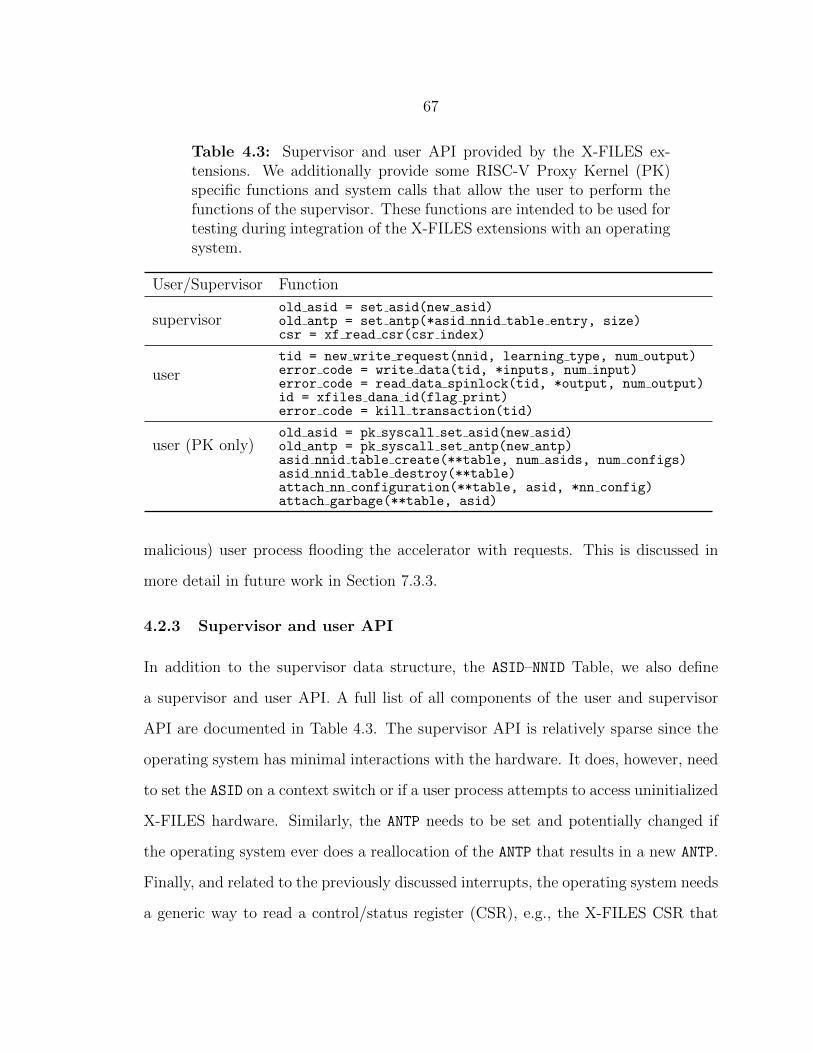
67
Table 4.3: Supervisor and user API provided by the X-FILES ex-tensions. We additionally provide some RISC-V Proxy Kernel (PK)specific functions and system calls that allow the user to perform thefunctions of the supervisor. These functions are intended to be used fortesting during integration of the X-FILES extensions with an operatingsystem.
User/Supervisor Function
supervisorold asid = set asid(new asid)old antp = set antp(*asid nnid table entry, size)csr = xf read csr(csr index)
usertid = new write request(nnid, learning type, num output)error code = write data(tid, *inputs, num input)error code = read data spinlock(tid, *output, num output)id = xfiles dana id(flag print)error code = kill transaction(tid)
user (PK only)old asid = pk syscall set asid(new asid)old antp = pk syscall set antp(new antp)asid nnid table create(**table, num asids, num configs)asid nnid table destroy(**table)attach nn configuration(**table, asid, *nn config)attach garbage(**table, asid)
malicious) user process flooding the accelerator with requests. This is discussed in
more detail in future work in Section 7.3.3.
4.2.3 Supervisor and user API
In addition to the supervisor data structure, the ASID–NNID Table, we also define
a supervisor and user API. A full list of all components of the user and supervisor
API are documented in Table 4.3. The supervisor API is relatively sparse since the
operating system has minimal interactions with the hardware. It does, however, need
to set the ASID on a context switch or if a user process attempts to access uninitialized
X-FILES hardware. Similarly, the ANTP needs to be set and potentially changed if
the operating system ever does a reallocation of the ANTP that results in a new ANTP.
Finally, and related to the previously discussed interrupts, the operating system needs
a generic way to read a control/status register (CSR), e.g., the X-FILES CSR that
68
holds that cause of an exception.4 Reading a CSR may have possible side effects like
clearing an outstanding interrupt from the X-FILES Hardware Arbiter.
At the user level, the X-FILE API is primarily concerned with initiating and
managing transactions using direct register transfer via the RoCC interface. In this
way a transaction can be broken down into three major steps:
• Transaction initiation
• Input vector (and expected output vector in the case of a learning transaction)
transfer to the X-FILES Hardware Arbiter
• Output vector transfer to the RISC-V microprocessor
This sequence of operations can be accomplished with the new write request,
write data, and read data spinlock functions of the user API. The TID for a given
transaction is generated by the X-FILES arbiter and returned after an invocation
of new write request. This TID is then repeatedly used by the user process to
communicate data back and forth with the X-FILES arbiter. The ASID is implicit
and the user process has no notion of its ASID nor has it any way to change its ASID.
The write data function can be used by the user process to communicate both an
input vector and an expected output vector if this is a learning transaction. For
learning transactions, the use of a non-unary batch size will result in the transaction
staying in the X-FILES Transaction Table for the lifetime of the batch. A new TID
will be issued by the X-FILES arbiter for each batch.
In addition to transaction instructions, we also provide operations for inspect-
ing the hardware. Information about the hardware can be requested using the
xfiles data id function. This function, in contrast to all others, can be invoked
without a valid ASID. Additionally, the user process can voluntarily kill a transaction
4The set asid and set antp could generally be viewed as a swap of a CSR and could be imple-mented as such.
69
with the kill transaction function.
4.3 Operating System Integration
While X-FILES hardware and software provides a supervisor API and associated data
structures, specifically, the ASID–NNID Table, these need to be properly integrated
with an operating system to be of practical use. For the purposes of this dissertation
we provide integration with two operating systems:
• The RISC-V Proxy Kernel, a lightweight kernel for running a single process and
developed by UC Berkeley [RISC-V Foundation, 2016b]
• The Linux Kernel RISC-V port [RISC-V Foundation, 2016a]
4.3.1 RISC-V Proxy Kernel
The Proxy Kernel requires limited modifications to integrate and evaluate X-FILES
hardware with an appropriate backend, e.g., DANA. Specifically, the extension bits,
(XS bits in the machine status/MSTATUS) must be set to a non-zero value. Since the
Proxy Kernel is, effectively, a uniprocessing kernel, there is no need to save and restore
the state of the X-FILES/backend as no other process will ever run.
For ease of use, we modify the Proxy Kernel with new system calls that allow a
user process to set the ASID and ANTP. This is not intended to be a final solution
(doing it this way in the Linux kernel would be inane), but these functions provide a
rough skeleton of what needs to be added to a multiprocessing operating system. By
introducing these system calls and adding functions for the creation, modification,
and deletion of the ASID–NNID Table, complete user applications can be developed
that avoid significant modifications to the Proxy Kernel.
Note, that it is beneficial to have the Proxy Kernel, and specifically the machine
mode portion of the Proxy Kernel, understand and panic when it sees an exceptional

70
case that generates a trap. We currently panic (with verbose information) on all
X-FILES/DANA-originating traps that machine mode catches. All modifications to
the Proxy Kernel are available as a patch to the RISC-V Proxy Kernel. This patch
can be accessed on the ICSG GitHub.
4.3.2 RISCV-V Linux port
The RISC-V Linux Port needs to be handled properly and we have taken great pains
to ensure that the model proposed by the X-FILES is correct, supports our multi-
transaction thesis, and that we integrate this with the kernel in a UNIX-like way.
Specifically, this requires the development of a device driver for the X-FILES Hard-
ware Arbiter specialized to the specific backend, e.g., DANA. Through this device
driver, which uses an associated ioctl, the user process can “write” a neural net-
work configuration. From the perspective of the user process, this appends that
neural network configuration to the ASID–NNID Table and returns the NNID where
that configuration is located.
However, a number of operations have to happen behind the scenes to ensure that
this operation is safe and that the memory is properly setup for X-FILES/DANA.
The device driver must first create an ASID–NNID Table if one does not exist. The
user process which initiated the ioctl write may, however, not have an associated
ASID. An ASID is then generated on the fly and will be stored with the task struct
for that user process on all future context switches. The ASID–NNID Table is modified
appropriately and the requested neural network configuration is stored in physical
memory for the NNID table associated with that user process’ ASID. The ASID–NNID
Table must exist as a physical memory data structure where all neural network con-
figurations are page-aligned. Additionally, all configurations must live on contiguous
pages if they span more than one page.5 This ensures safe, easy, and fast operation
5The default page size for RISC-V is 4KB.
71
of the underlying hardware when performing a read or write to or from the ASID–
NNID Table. Consequently, on an ioctl write, the device driver must verify that the
user process has provided sane data, create a new entry in the ASID–NNID Table if
needed, and grab and pin enough contiguous pages where the specified neural network
configuration will live.
The importance of using pinned memory is that once the operating system gives
the hardware an ANTP, it cannot touch any of the pages associated with that during
normal virtual memory management. Without this, the operating system could pull
a page belonging to the ASID–NNID Table which would cause the hardware to read or
write some region of memory that it is not supposed to. This would likely destabilize
the entire system, but is also a security vulnerability.
Outside of the development of this device driver, the operating system needs to
take all the appropriate actions to keep whatever new state properly associated with
a process. Specifically, the task struct needs to keep track of the ASID for a given
process. We use a default value of −1 to indicate an invalid ASID (which will be
loaded into the X-FILES Hardware Arbiter on a context switch). This allows the
hardware to generate an interrupt when a user process that does not have an ASID
tries to access an accelerator for the first time. Relatedly the Linux kernel must be
modified to at least recognize the interrupts that the hardware could generate. Note,
that due to the nature of the RISC-V privileged specification, interrupts drop the
microprocessor into machine mode. The machine mode then has the ability to defer
these interrupts to be handled in a different mode, i.e., the hypervisor, supervisor
(operating system), or the user.
These modifications, while described here, are currently in the process of being
fully implemented. We comment on their progress in Section 7.3.5.
72
4.4 Summary
In summary, the X-FILES extensions define hardware and software to manage neural
network transactions within the framework of a multiprocessing operating system like
the Linux kernel. We have taken extreme pains to make certain that the model pro-
posed here is sound and accurately meets the needs of our multi-transaction model and
motivating applications in the approximate computing [Esmaeilzadeh et al., 2012b]
and automatic parallelization [Waterland et al., 2014] domains. Similarly, the de-
sign of X-FILES hardware has undergone many revisions with one notable revision
involving the complete separation of all X-FILES and backend accelerator hardware.
For this reason, the X-FILES provide agnosticity to the backend and can support
multi-context, single-context, and combinational logic backends.
However, the X-FILES forms only one part of the picture—the X-FILES expect
to have a defined and implemented backend capable of doing useful work. For this
reason, and to further evaluate the proposed work of the X-FILES, we describe in
Section 5 our implementation of DANA, a neural network accelerator suitable for
approximate computing or automatic parallelization applications and aligning with
our multi-transaction model of computation.
73
Chapter 5
DANA: An X-FILES Accelerator for
Neural Network Computation
Previously, we provided a discussion of the X-FILES, hardware and software ex-
tensions for the management of neural network transactions, i.e., requests by user
processes to access neural network accelerator hardware. However, and as previously
mentioned, the X-FILES only form one part of a complete system. A complete system
requires an X-FILES backend that provides the computational capabilities required
to make forward progress on transactions. This backend can be multi-context, single-
context, or no-context (i.e., strictly combinational logic) and this choice is left to the
discretion of the designer of an X-FILES backend. Nonetheless, we focus primarily
on multi-context usage and develop a new architecture for accelerating neural net-
work computation that interfaces seamlessly with X-FILES hardware and software
and supports our multi-transaction model of computation. Our resulting multilayer
perceptron neural network backend, DANA, demonstrates the capabilities of the X-
FILES, aligns with the needs of our motivating applications, and provides a platform
on top of which we evaluate our multi-transaction model in Chapter 6.
In the following sections we provide a more lengthy motivation for the specifics of
this DANA architecture. We then provide a full description of DANA as well as its
operation in both feedforward inference and gradient descent learning tasks.
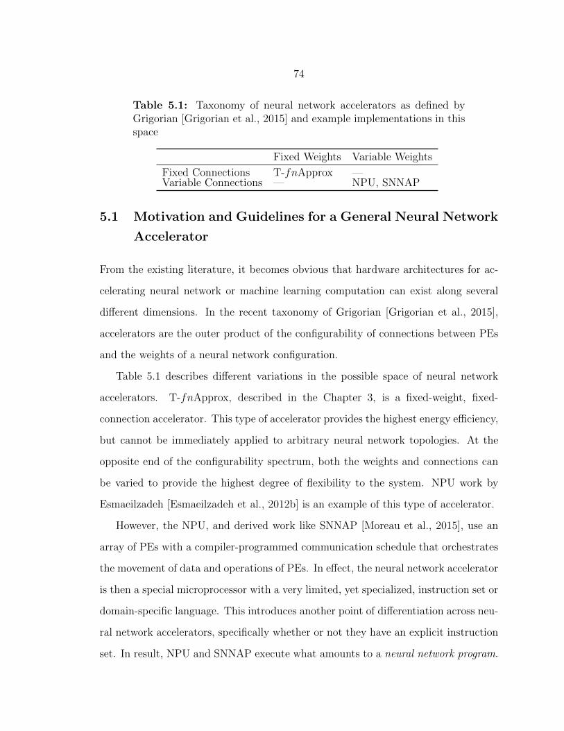
74
Table 5.1: Taxonomy of neural network accelerators as defined byGrigorian [Grigorian et al., 2015] and example implementations in thisspace
Fixed Weights Variable Weights
Fixed Connections T-fnApprox —Variable Connections — NPU, SNNAP
5.1 Motivation and Guidelines for a General Neural Network
Accelerator
From the existing literature, it becomes obvious that hardware architectures for ac-
celerating neural network or machine learning computation can exist along several
different dimensions. In the recent taxonomy of Grigorian [Grigorian et al., 2015],
accelerators are the outer product of the configurability of connections between PEs
and the weights of a neural network configuration.
Table 5.1 describes different variations in the possible space of neural network
accelerators. T-fnApprox, described in the Chapter 3, is a fixed-weight, fixed-
connection accelerator. This type of accelerator provides the highest energy efficiency,
but cannot be immediately applied to arbitrary neural network topologies. At the
opposite end of the configurability spectrum, both the weights and connections can
be varied to provide the highest degree of flexibility to the system. NPU work by
Esmaeilzadeh [Esmaeilzadeh et al., 2012b] is an example of this type of accelerator.
However, the NPU, and derived work like SNNAP [Moreau et al., 2015], use an
array of PEs with a compiler-programmed communication schedule that orchestrates
the movement of data and operations of PEs. In effect, the neural network accelerator
is then a special microprocessor with a very limited, yet specialized, instruction set or
domain-specific language. This introduces another point of differentiation across neu-
ral network accelerators, specifically whether or not they have an explicit instruction
set. In result, NPU and SNNAP execute what amounts to a neural network program.

75
An alternative approach, and what we explore with our DANA architecture, uses
a neural network configuration. This neural network configuration is a data structure
that describes the structure of the neural network (and similar to the approach of
Grigorian [Grigorian et al., 2015]). While the concept of a neural network program
and a neural network configuration as fungible (i.e., they are functionally equivalent),
a configuration exposes more semantic information to the hardware and potentially
allows for a more efficient utilization of the underlying hardware resources.1 Relatedly,
while a neural network program does not preclude SMT of neural networks, the use
of a neural network configuration provides a more concise structure for the units of
computation to enable accelerator multiprocessing more elegantly.
As outlined in the motivation sections of this thesis, the large first derivative of
neural network and machine learning computation can be used as an indicator of
widespread adoption of this soft computing model. We argue that machine learning
is not something relegated to its own application domain. Exposing generic learning
and inference as computational primitives provides substantial benefits to applications
in a general sense. With this in mind, we design a machine learning accelerator
architecture that naturally supports difficult hardware concepts like SMT. Hence,
the use of a neural network configuration forms one of the tenets of our architectural
design choice.
Similarly, while a fixed accelerator suited for just one specific neural network may
find use within an Internet of Things (IoT) application, neural network accelerators
need to support both variations in topology and in the weights of constituent connec-
tions. For these reasons, we extend the initial T-fnApprox architecture to support
1An equivalent comparison would be a graph processing algorithm represented as data movementinstructions between nodes or hardware for graph processing that understands how to read andwrite an adjacency list. The latter approach exposes significantly more semantic information to theprocessing hardware. A similar example involves the trade-offs of just-in-time (JIT) compilation vs.ahead-of-time (AOT) compilation.
76
arbitrary topologies specified using neural network configurations.
Related to the motivating applications, approximate computing and automatic
parallelization, and either their expected wide adoption or taking the view that these
are representative of future applications that liberally incorporate machine learning,
we design DANA with the following properties:
• We optimize DANA for the temporal reuse of neural network configurations
• We make DANA multi-context and capable of executing a parameterized number
of simultaneous transactions
With regard to the former point, this builds off of the observations of Esmaeilzadeh
that approximation via neural networks should be applied to frequently used, hot
functions [Esmaeilzadeh et al., 2012b]. In effect, if the functions are hot, then the
neural network configuration will also be hot. Hence, any accelerator intended to
work in this niche area of approximation should be capable of caching neural network
configurations (or programs if the accelerator is so designed) since the approximated
functions are, by transitivity, hot. A similar argument holds for automatic paral-
lelization applications. In these applications, neural networks are used to infer the
future state2 of a microprocessor [Waterland et al., 2014].
With regard to the latter point of a need for multi-context support, this has
several motivations. First, in light of the aforementioned motivating applications,
the frequent use of neural networks as approximators or state predictors necessitates
hardware that can cope with neural network transactions being frequently generated.
Second, as machine learning becomes a generic component of applications as opposed
to the application, we envision a computational world where neural networks are used
2By state we mean the entire state of the microprocessor: registers, memory (including inputsstored in memory), and disks. The microprocessor is then viewed from a dynamical systems per-spective as defining a discrete transformation from the state of the system at the current time step,tt, to the next time step, tt+1. The predictions occur from the same initial point in the state spaceand, consequently, use the same neural network repeatedly.

77
by all user processes and the operating system. As a result, the hardware must be able
to cope with disparate processes simultaneously generating neural network transac-
tions. Third, the multi-context nature, while requiring significant architectural design
at the hardware and software levels as evidenced by the X-FILES work presented in
Chapter 4, exposes more parallel work to the underlying hardware accelerator. This
has the potential to improve the throughput of the accelerator in the same manner
that SMT does for modern microprocessors.
In summary, we architect DANA as an accelerator that understands neural net-
work configurations and, through the use of local caching of neural network configura-
tions, takes advantage of neural network temporal locality. Furthermore, we explicitly
architect DANA to be capable of multi-transaction operation.
5.2 DANA: A Dynamically Allocated Neural Network Ac-
celerator
DANA, an acronym for Dynamically Allocated Neural Network Accelerator, has
already been introduced with limited commentary in Figure 4·3 as an accelerator
backend for the X-FILES. Note that the dynamic allocation properties of DANA are
in reference to the dynamic allocation of its PEs. DANA is composed of six major
architectural components that are briefly listed below:
• A DANA-specific Transaction Table3
• A Configuration Cache
• An ASID–NNID Table Walker
• Control logic
• A parameterized number of PEs
3Note: this is different, but related to the X-FILES Transaction Table. More commentary followsin the main body.
78
• Per-transaction scratchpad memories
The following subsections provide a discussion of each of these components.
5.2.1 Transaction Table
The immediate question is: why does DANA include a Transaction Table when the X-
FILES Hardware Arbiter already provides one? Recall that the X-FILES Transaction
Table only stores information about a transaction related to whether or not that
entry in the X-FILES Transaction Table is valid (the reserved/R bit), its ability to
be scheduled on the backend accelerator (the VDIO bits), and its identification (an
ASID–TID tuple). Nothing about the fine-grained state of the transaction is stored,
e.g., what is the next neuron to be scheduled.4 This aligns with the model put forth
in the discussion of the X-FILES Hardware Arbiter. Namely, if the backend (e.g.,
DANA) wants to be multi-context, it needs to introduce some architectural features
that allow state to be maintained.
For DANA, we use a Transaction Table of the same number of entries as the X-
FILES Transaction Table. The fields of DANA’s Transaction Table are broken down
into three regions: a valid bit, an NNID, and transaction state. The valid bit indicates
to DANA’s control logic that this transaction has valid data. The NNID provides
an identifier that allows DANA to traverse the ASID–NNID Table to find a specific
neural network configuration. For this reason, the NNID is DANA-specific. DANA’s
Transaction Table also records the transaction state in a long vector. While the full
contents of the state vector are not discussed herein (the curious reader can examine
the actual source HDL), the pertinent points are discussed below.
The transaction state must keep track of what work has been done and what
work needs to be done. Generally, though discussed in more detail in Sections 5.3.1
4Early versions of X-FILES/DANA had a unified Transaction Table [Eldridge et al., 2015]. Duringa refactor attempting to completely separate X-FILES hardware from DANA the current divisionof Transaction Tables was developed.
79
and 5.3.2, the state involves tracking what layer and what neuron within a layer is the
next to be processed. Additionally, the type of the transaction (feedforward inference
or learning with a specific batch size) dramatically changes the state transitions that
the underlying hardware goes through to move a transaction to completion. Certain
one time use checks are stored in the transaction state. These include whether or not
the transaction is eligible to be scheduled (set by the X-FILES Hardware Arbiter),
whether the specific NNID is currently cached, and derived parameters that are a
function of the current layer and neuron (pointers for data locations in the neural
network configuration).
Whenever DANA’s Transaction Table comes across a situation that requires wait-
ing for some information from the X-FILES arbiter (e.g., the transaction needs inputs,
but the input queue is empty), DANA communicates to the X-FILES arbiter to de-
schedule the waiting transaction. This type of action results in one of the VDIO bits
in the X-FILES Transaction Table being set. When the X-FILES arbiter receives an
action from the microprocessor that remedies this condition, then the transaction will
be rescheduled and re-enabled on DANA.
DANA’s Transaction Table internally arbitrates between transactions which have
work to do. The Transaction Table determines the next action to take and generates
a request to DANA’s Control Module. Once the transaction has finished execution
and all output data has been sent to an X-FILES Hardware Arbiter output queue,
DANA’s Transaction Table responds to the X-FILES arbiter causing the done (D) bit
to be set. This allows incident read data spinlock requests to succeed and data to
be sent back to the requesting process.
5.2.2 Configuration Cache
As previously mentioned, neural network configurations are stored locally in a Con-
figuration Cache. This caching allows us to exploit the temporal locality of our target
80
applications. The Configuration Cache has a parameterized number of entries, stored
in a table, corresponding to the number of configurations that can be stored at a
given time. Each entry in the cache also has a corresponding memory block where
the configuration will be stored as it is read in from the memory hierarchy of the
attached RISC-V microprocessor.
Figure 5·1 shows the structure of a neural network configuration. A configuration
is composed of four regions containing information pertaining to a different part of
the neural network:
• Global information
• Per-layer information
• Per-neuron information
• The weights
Each of these regions contains pointers to other areas that allow processing of the
neural network to proceed, e.g., the per-layer information contains a pointer to the
first neuron of a layer. DANA’s Transaction Table can then use this information to
provide a PE with the location of its specific neuron configuration. Analogously, the
per-neuron region contains pointers into the weight region so that a PE can locate
and load the weights that it needs to perform its input–weight inner product.
Similar to how a transaction can be uniquely identified with an ASID–TID tuple,
a neural network configuration can be uniquely identified with an ASID–NNID tuple.
When DANA’s Transaction Table generates a request for a specific neural network
configuration to the Configuration Cache, this request contains that ASID–NNID tuple.
The cache does a parallel comparison on all valid entries in the cache. The result
of this comparison is effectively a cache hit or miss—the requested neural network
configuration is found or not found in the list of cached entries.
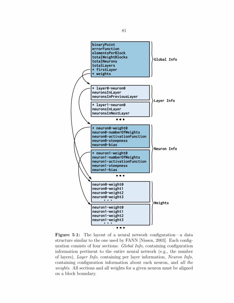
81
binaryPointerrorFunctionelementsPerBlocktotalWeightBlockstotalNeuronstotalLayers* firstLayer* weights
Global Info
Weights
* neuron0-weight0neuron0-numberOfWeightsneuron0-activationFunctionneuron0-steepnessneuron0-bias
Neuron Info
* layer0-neuron0neuronsInLayerneuronsInPreviousLayer
* layer1-neuron0neuronsInLayerneuronsInNextLayer
Layer Info
* neuron1-weight0neuron1-numberOfWeightsneuron1-activationFunctionneuron1-steepnessneuron1-bias
neuron0-weight0neuron0-weight1neuron0-weight2neuron0-weight3...
neuron1-weight0neuron1-weight1neuron1-weight2neuron1-weight3...
Figure 5·1: The layout of a neural network configuration—a datastructure similar to the one used by FANN [Nissen, 2003]. Each config-uration consists of four sections: Global Info, containing configurationinformation pertinent to the entire neural network (e.g., the numberof layers), Layer Info, containing per layer information, Neuron Info,containing configuration information about each neuron, and all theweights. All sections and all weights for a given neuron must be alignedon a block boundary.
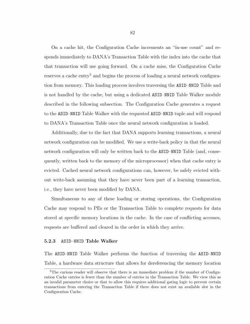
82
On a cache hit, the Configuration Cache increments an “in-use count” and re-
sponds immediately to DANA’s Transaction Table with the index into the cache that
that transaction will use going forward. On a cache miss, the Configuration Cache
reserves a cache entry5 and begins the process of loading a neural network configura-
tion from memory. This loading process involves traversing the ASID–NNID Table and
is not handled by the cache, but using a dedicated ASID–NNID Table Walker module
described in the following subsection. The Configuration Cache generates a request
to the ASID–NNID Table Walker with the requested ASID–NNID tuple and will respond
to DANA’s Transaction Table once the neural network configuration is loaded.
Additionally, due to the fact that DANA supports learning transactions, a neural
network configuration can be modified. We use a write-back policy in that the neural
network configuration will only be written back to the ASID–NNID Table (and, conse-
quently, written back to the memory of the microprocessor) when that cache entry is
evicted. Cached neural network configurations can, however, be safely evicted with-
out write-back assuming that they have never been part of a learning transaction,
i.e., they have never been modified by DANA.
Simultaneous to any of these loading or storing operations, the Configuration
Cache may respond to PEs or the Transaction Table to complete requests for data
stored at specific memory locations in the cache. In the case of conflicting accesses,
requests are buffered and cleared in the order in which they arrive.
5.2.3 ASID–NNID Table Walker
The ASID–NNID Table Walker performs the function of traversing the ASID–NNID
Table, a hardware data structure that allows for dereferencing the memory location
5The curious reader will observe that there is an immediate problem if the number of Configu-ration Cache entries is fewer than the number of entries in the Transaction Table. We view this asan invalid parameter choice or that to allow this requires additional gating logic to prevent certaintransactions from entering the Transaction Table if there does not exist an available slot in theConfiguration Cache.

83
of a neural network configuration from an ASID–NNID tuple. The ASID–NNID Table
was discussed previously in Section 4.2.2 and is shown in Figure 4·4.
The ASID–NNID Table Walker contains a hardware state machine for walking this
table using the uncached L2 port of the RoCC interface. While initial versions of
this hardware unit used cached L1 accesses, the neural network configurations have
no legitimate reason to pass through the L1 data cache of the microprocessor. The
reason for this is that there exists no foreseeable temporal or spatial reuse of these
configurations by the microprocessor. Passing these configurations through the L2
cache avoids polluting (and likely completely clearing) the L1 data cache.
In effect, the ASID–NNID Table Walker is a hardware page table walker except
the data structure is an ASID–NNID Table instead of a page table. As it is possible
for the Configuration Cache to have multiple outstanding load or store requests, the
ASID–NNID Table Walker queues pending requests by the Configuration Cache. Loads
are prioritized over stores, assuming that the loads have a destination that does not
require write-back, to provide minimal latency to outstanding transactions.
Due to the ASID–NNID Table Walker interacting directly with memory, there exist
numerous ways that loads or stores can fail. For example, there is no guarantee that
the user will provide a valid NNID (the NNID could be outside the bounds of the ASID–
NNID Table). This results in an X-FILES backend exception that the microprocessor
will have to handle. An exhaustive list of all exceptions that DANA can generate
(which will result microprocessor interrupts) are shown in Table 4.2.
5.2.4 Control module
DANA’s control module largely provides routing of signals from and to different mod-
ules internal to DANA. Most modules operate entirely independently of each other in
the sense that they use asynchronous interfaces to generate requests to other modules
when those modules are available and react to inbound requests. However, DANA
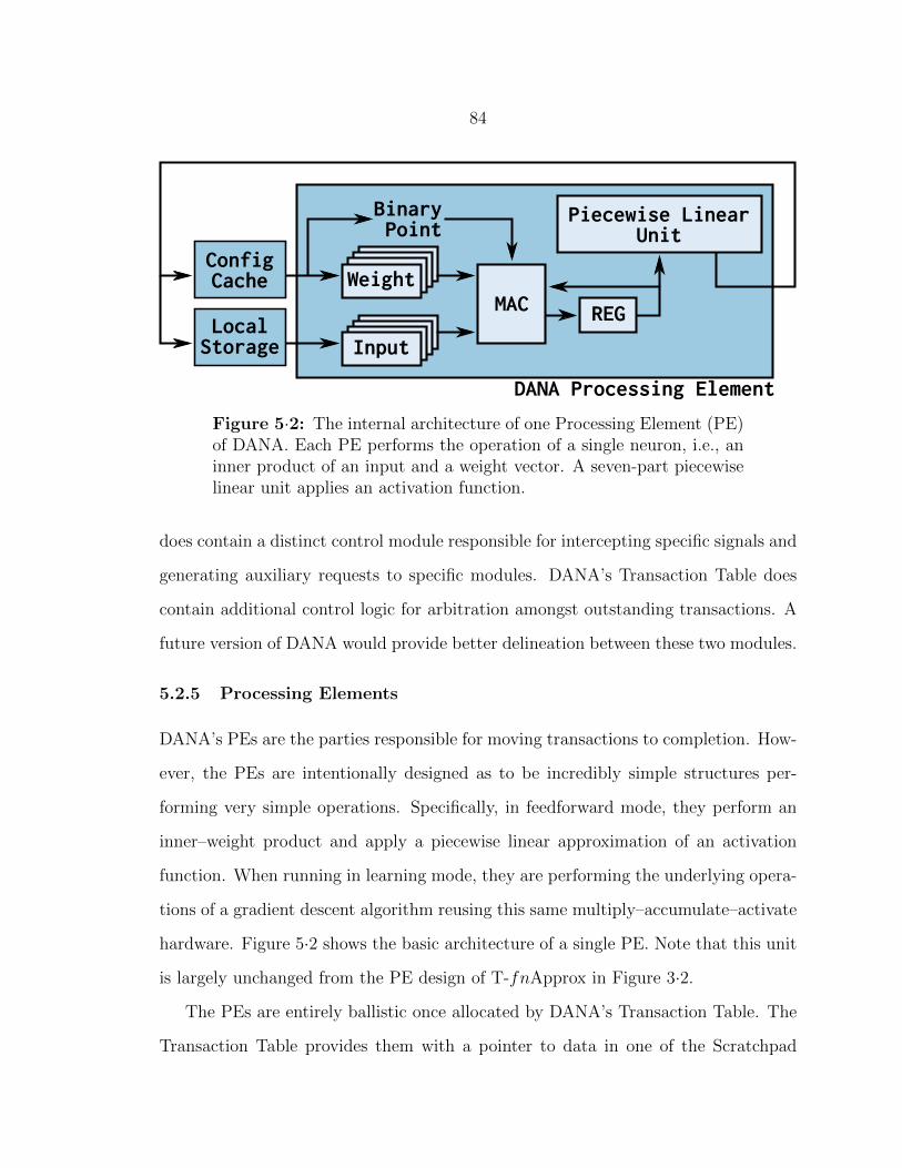
84
Input
Weight
MAC
BinaryPoint
REG
Piecewise LinearUnit
ConfigCache
LocalStorage
DANA Processing Element
Figure 5·2: The internal architecture of one Processing Element (PE)of DANA. Each PE performs the operation of a single neuron, i.e., aninner product of an input and a weight vector. A seven-part piecewiselinear unit applies an activation function.
does contain a distinct control module responsible for intercepting specific signals and
generating auxiliary requests to specific modules. DANA’s Transaction Table does
contain additional control logic for arbitration amongst outstanding transactions. A
future version of DANA would provide better delineation between these two modules.
5.2.5 Processing Elements
DANA’s PEs are the parties responsible for moving transactions to completion. How-
ever, the PEs are intentionally designed as to be incredibly simple structures per-
forming very simple operations. Specifically, in feedforward mode, they perform an
inner–weight product and apply a piecewise linear approximation of an activation
function. When running in learning mode, they are performing the underlying opera-
tions of a gradient descent algorithm reusing this same multiply–accumulate–activate
hardware. Figure 5·2 shows the basic architecture of a single PE. Note that this unit
is largely unchanged from the PE design of T-fnApprox in Figure 3·2.
The PEs are entirely ballistic once allocated by DANA’s Transaction Table. The
Transaction Table provides them with a pointer to data in one of the Scratchpad
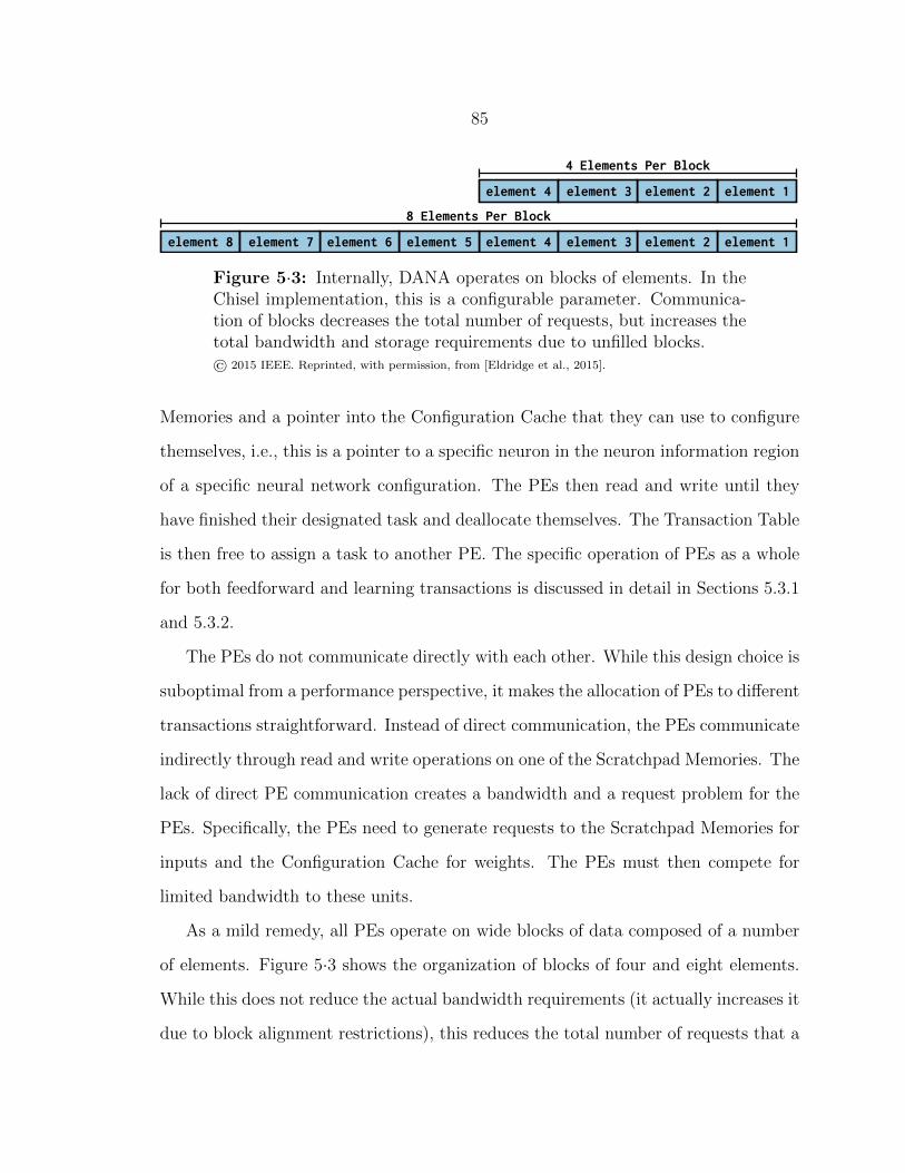
85
4 Elements Per Block
element 4 element 3 element 2 element 1
8 Elements Per Block
element 8 element 7 element 6 element 5
element 4 element 3 element 2 element 1
Figure 5·3: Internally, DANA operates on blocks of elements. In theChisel implementation, this is a configurable parameter. Communica-tion of blocks decreases the total number of requests, but increases thetotal bandwidth and storage requirements due to unfilled blocks.© 2015 IEEE. Reprinted, with permission, from [Eldridge et al., 2015].
Memories and a pointer into the Configuration Cache that they can use to configure
themselves, i.e., this is a pointer to a specific neuron in the neuron information region
of a specific neural network configuration. The PEs then read and write until they
have finished their designated task and deallocate themselves. The Transaction Table
is then free to assign a task to another PE. The specific operation of PEs as a whole
for both feedforward and learning transactions is discussed in detail in Sections 5.3.1
and 5.3.2.
The PEs do not communicate directly with each other. While this design choice is
suboptimal from a performance perspective, it makes the allocation of PEs to different
transactions straightforward. Instead of direct communication, the PEs communicate
indirectly through read and write operations on one of the Scratchpad Memories. The
lack of direct PE communication creates a bandwidth and a request problem for the
PEs. Specifically, the PEs need to generate requests to the Scratchpad Memories for
inputs and the Configuration Cache for weights. The PEs must then compete for
limited bandwidth to these units.
As a mild remedy, all PEs operate on wide blocks of data composed of a number
of elements. Figure 5·3 shows the organization of blocks of four and eight elements.
While this does not reduce the actual bandwidth requirements (it actually increases it
due to block alignment restrictions), this reduces the total number of requests that a
86
E[output]Input
Hidden1 OutputHidden2 Output
HiddenN OutputOutput
Feedforward Computation
Output δ-Weight SumHiddenN δ-Weight Sum
Hidden2 δ-Weight Sum
Bias Updates Hidden1Bias Updates Hidden2
Bias Updates HiddenN
Weight Updates
Error Backpropagation
Scratchpad Memory
GradientDescent
Learning
3 4 5
1 2
B
B
1 2 3
4 5
B
B
FeedforwardInference
PassThroughInput
Neurons
Bias NeuronsAccumulated Weight Updates
ConfigurationCache
ASID NNID State
CacheMemory Post-Batch
Weight UpdatesDana Accelerator
Figure 5·4: A per-transaction Scratchpad Memory and the move-ment of data involving reads and writes by DANA’s Processing Ele-ments (PEs) for both feedforward inference and gradient descent learn-ing transactions.
PE will generate. All data in the Configuration Cache and Scratchpad Memories must
then be block aligned to avoid the overhead of misaligned reads requiring multiple
reads to complete a single request.
5.2.6 Scratchpad memories
DANA provides intermediate storage and, implicitly, PE communication through per-
transaction scratchpad memories. Figure 5·4 shows one such scratchpad memory and
the breakdown of data internal to it. At a high level, each scratchpad is broken
into three logical regions. The top region contains information related to feedforward
computation. Note that a feedforward transaction does not have expected outputs
(E[output])—the input region is shifted up to the fill this spot. The middle region
contains information related to error backpropagation. The bottom region contains
87
accumulated weight updates for learning transactions with a batch size larger than
one.
The element–block organization discussed previously introduces some difficulties
for proper organization and use of the scratchpad memories. Specifically, in feedfor-
ward computation, each PE computes one element of a block. Similarly, during a
learning transaction, each PE computes a partial delta–weight product which must
be accumulated directly in the scratchpad memory.
In response, we introduce several modifications to a traditional memory unit to
enable element-wise writes and in-memory accumulations. Each write to a memory
location can be one of the following operations:
• Element-wise, overwriting old data (feedforward operation generating an output)
• Element-wise, accumulating with old data (learning with accumulation of a
delta–weight product)
• Whole-block, overwriting old data (a weight block that is from the first unit of
a batch)
• Whole-block, accumulating element-wise with old data (a weight block not the
first unit of a batch)
We accomplish this using a two-stage read-modify-write operation with input
forwarding to cover the case of back to back writes to the same block. This style
of memory architecture bears similarities to architectures supporting atomic memory
operations and read/write masks. Alternatively, a different DANA architecture that
used direct PE communication (via, e.g., PE output broadcast, an explicit PE routing
network, or a systolic array of PEs) would remove the necessity of this scratchpad
memory design.
Due to the need for a learning operation to overlay the weight updates from a
scratchpad memory on the Configuration Cache, we reuse this memory hardware for

88
the Configuration Cache memories.
5.3 Operation for Neural Network Transactions
We now provide an overview of how both feedforward and gradient descent learning
works and how it is implemented on DANA. Figure 5·4 shows the logical operation
of DANA for a learning transaction (which includes feedforward computation).
5.3.1 Feedforward computation
DANA computes an output vector for a given input vector. The input vector is
communicated to the scratchpad memory for that transaction through the X-FILES
Hardware Arbiter’s input queue. During this process, the Configuration Cache and
the ASID–NNID Table Walker are working together to load the correct neural network
configuration if it is not already present.
Once the data is loaded and the neural network configuration is available, DANA’s
Transaction Table begins allocating neurons in the first hidden layer. Neurons are
allocated left to right, as shown with the counts in the Feedforward Inference block
of Figure 5·4. Each PE is responsible for applying an activation function, σ, to an
inner–weight product:
y =∑∀weights
weight× input (5.1)
z = σ (y) (5.2)
Each PE may require multiple reads from the Configuration Cache and the scratch-
pad memory to sequentially load all the weights and inputs. After the computation
of the activation function, the PE writes its output to the scratchpad memory. All
PEs for the first hidden layer neurons perform this process in parallel. Once all PEs
have written their outputs to the scratchpad memory, the scratchpad memory noti-
89
fies the Transaction Table that all outputs are available and the next layer can begin
processing.
This process repeats for all neurons in the neural network until a final output
vector is computed. Following this, the transaction is done and the output vector is
loaded into an output queue of the X-FILES Hardware Arbiter where a user process
will grab the data. Once the output queue has been emptied, the transaction is
removed from all the Transaction Tables and that entry can be reused for a new
transaction.
5.3.2 Learning
Learning involves modifying the weights of inter-neuron connections in an attempt to
minimize an output cost function like mean squared error (MSE). The challenge of
learning is then rapidly determining the relative contribution of each weighted con-
nection towards this cost function, i.e., the partial derivative of the cost function with
respect to each weight. By deliberately choosing differentiable activation functions,
output derivatives (or errors) backpropagate through the network in a single backward
sweep, much faster than via the chain rule. In the update step, weights are moved
against their individually computed derivatives to, ideally, decrease the cost function.
A learning transaction starts where a feedforward transaction ends, right when a
PE performing the functions of an output neuron computes an output. This neuron
then computes the error (the difference between the expected value and the computed
value for that neuron only) and uses this to compute the derivative of the error. Each
output neuron reads its expected output value, E[zout], from a Scratchpad Memory,
and computes its output error, E[zout] − zout, and cost function derivative, δ. This
derivative requires the activation function derivative, σ′, which can be defined in
terms of known parameters for a sigmoid (Equation 5.3). Note that to align with
FANN we apply an inverse hyperbolic tangent function that amplifies the output
90
error (Equation 5.4):
σ′sigmoid(y) = σsigmoid(y)× (1− σsigmoid(y)) (5.3)
δout = σ′ (yout) atanh(E[zout]− zout) (5.4)
Output derivatives are broadcast backwards along the input connections of an out-
put neuron, multiplied by their connection weights, and accumulated at the previous
layer nodes (see Equation 5.5). This is accomplished through the aforementioned
in-memory accumulation hardware of the scratchpad memories. Scaled by the acti-
vation function derivative, σ′, this product forms the cost function derivative for each
hidden node in the previous layer i− 1:
δhiddeni−1= σ′
(yhiddeni−1
) ∑∀weights
δouti × weighti (5.5)
Weight accumulation
During the gradient descent learning phase of a learning transaction, each PE will
also generate a weight update, ∆w, by multiplying the neuron-specific cost function
derivative, δ, by the current input seen along that connection:
∆w = δ × input (5.6)
In the case of stochastic gradient descent, this weight update will be immediately
used to update the old weight stored in the Configuration Cache (see below). For
gradient descent learning (or if some batch size is used), partial weight updates are
accumulated in a Scratchpad Memory over some number of input–output pairs before
being used to update the old, cached weight. Bias updates or partial bias updates
are similarly computed.
91
Weight update
All accumulated partial weight updates are finally scaled by a user-specified learning
rate (divided by the batch size) and added to the old weight value:
weight = old weight +learning rate
# training pairs×
∑∀training pairs
∆w (5.7)
In consequence, on completion of a batch, the accumulated partial weight and bias up-
dates in the scratchpad memory are used to update the neural network configuration
in the Configuration Cache.
5.4 Summary
Here, we provide the architectural description of DANA, a multilayer perceptron
neural network accelerator that acts as a multi-transaction backend for the X-FILES
hardware and software extensions. Together, X-FILES/DANA can be used to aug-
ment a RISC-V microprocessor and enable hardware acceleration of both feedforward
inference and gradient descent learning transactions. Our evaluation of this com-
bined system is discussed in more detail in Chapter 6. All HDL and source code for
X-FILES/DANA hardware and software is available on the Boston University Inte-
grated Circuits and Systems group GitHub [Boston University Integrated Circuits and
Systems Group, 2016]. Using the open source Rocket Chip GitHub repository [UC
Berkeley Architecture Research Group, 2016], a complete Rocket + X-FILES/DANA
system can be emulated in software or evaluated in FPGA hardware.
92
Chapter 6
Evaluation of X-FILES/DANA
This chapter summarizes existing and new evaluations of DANA and X-FILES/DANA
during the various stages of development that this project has undergone. We first
provide a description of the various work and implemented versions of this system and
then delve into DANA-specific analysis followed by evaluation of a complete RISC-V
microprocessor (Rocket) + X-FILES/DANA.
6.1 Different Implementations of X-FILES/DANA
There currently exist three implementations that incorporate some version of DANA:
• A C++ model of DANA
• A SystemVerilog version of X-FILES/DANA accessed via a Universal Asyn-
chronous Receiver/Transmitter (UART) wrapper
• A Chisel [Bachrach et al., 2012] version of X-FILES/DANA integrated with
a RISC-V microprocessor [Boston University Integrated Circuits and Systems
Group, 2016]
The C++ model was only used for initial design space exploration of the archi-
tecture and is not specifically evaluated in this section. However, it is important to
comment on some of the lessons learned during this exploratory design phase that
impacted the SystemVerilog and Chisel versions.
First, this version (and the SystemVerilog version) uses a Register File composed
93
of blocks of elements for intermediate storage (as opposed to the Chisel version that
uses Scratchpad Memories). Figure 6·1 shows this Register File architecture. At the
time, only inference transactions were considered and these required substantially less
intermediate storage space than learning transactions. However, this Register File,
which also uses DANA’s block of elements data organization (see Figure 5·3), needs
to store vectors of data larger than a single block. To remedy this, the Register File
uses a linked list-like structure to logically connect blocks in the Register File. Each
entry in the Register File contains a “next” pointer, fields with the number of used
(written to) entries, and a “last” bit. The next pointer defines the entry of the next
block in a sequence, the number of used entries prevents a PE from reading invalid
data, and the last bit defines when a PE has read all the inputs it needs to.
This structure, while workable, is overly complicated and unsuitable for learning
transactions that produce abundant intermediate data. Additionally, the use of this
Register File architecture slows down the rate of PE allocation as the Control Module
must reserve entries in the Register File before PEs can be allocated. Without this
reservation step, PEs can deadlock if they have no output location in the Register File
to write to. While the Register File approach was used for the subsequent SystemVer-
ilog implementation, this was eventually abandoned in the Chisel implementation for
dedicated per-transaction Scratchpad Memories.
Second, the C++ model provided early indications that exposing multiple, simul-
taneous neural network transactions to DANA improved DANA’s overall throughput.
This result, quantified for the SystemVerilog implementation in subsequent sections,
is not surprising, however. Exposing multiple neural network transactions allows
DANA to utilize the explicit parallelism of multiple, independent transactions to dy-
namically avoid read after write (RAW) dependencies that cause a single transaction
to stall.

94
Data to store:
R0 R1 R2 R3
R4 R5 R6 R7
R8 R9 R10 R11
R12 R13 R14 R15
Block0
Block1
Block2
Block3
Block2
Pointer
4
2
3-1
-1
1
1
1
0 -1 -1
Register File
RegistersValid #Used
isLast
0
1
1
-1
Figure 6·1: Register File (left) used to store two groups of inter-mediate data (right) in initial DANA implementations and used forSection 6.2 evaluations. The Register File uses the block of elementsstructure of DANA (see Figure 5·3) with the Register File shown abovehaving four blocks of four elements (or registers) each. Data largerthan a single block, e.g., blue “data to store” (right), spans multipleRegister File blocks (block0 and block2). A pointer indicates the nextblock in such a sequence and a #Used field and isLast bit allow for par-tially filled blocks and determination of the last block and element ina sequence. This architecture is not, however, suitable for storing largeamounts of data (e.g., for learning transactions) and, consequently, wasreplaced by per-transaction Scratchpad Memories (see Figure 4·3 andSection 5.2.6) in later DANA versions.

95
This C++ model was integrated with the gem5 system simulator [Binkert et al.,
2011], but was not ultimately used for evaluations. We replicated the load/store
unit of gem5 to create an accelerator load/store unit. Using additional x86 assembly
instructions, we were then able to use DANA, integrated directly with this load/store
unit to accelerate neural network computation. The interface, at this time, was a
simple write/read pair composed of two instructions: ACCWRITE and ACCREAD (cf.
their eventual successors write data and read data spinlock in Table 4.3). These
could be used to write an input vector to DANA and, after processing, read the
output vector. Neural network configurations were preloaded into the Configuration
Cache and not loaded through the write/read interface.
Nonetheless, we deemed it prudent to focus on an actual hardware implementation
of DANA. Consequently, the gem5 + DANA implementation was not specifically used
for any extensive evaluation.
6.2 X-FILES/DANA in SystemVerilog
Following this prototyping exercise of a C++ version of DANA integrated with gem5,
we implemented X-FILES/DANA1 in SystemVerilog. This approach did not deviate
dramatically from the architecture developed during the C++ prototype phase and
broadly speaks to the utility of software prototyping before hardware implementation.
At this time, the delineation between the X-FILES Hardware Arbiter and DANA
was not clearly defined, e.g., there was a single, unified Transaction Table inter-
nal to the Hardware Arbiter. Consequently, the Hardware Arbiter was not suit-
ably designed for backends differing from DANA. Figure 6·2 shows the architectural
diagram for the SystemVerilog implementation of X-FILES/DANA. Note that the
ASID–NNID Table Walker, ASID units, and Transaction Queue were defined in the
1During this time the separation of transaction management hardware (the X-FILES HardwareArbiter) and the backend accelerator (DANA) began to take shape.

96
ASID-NNIDTableWalker
ASID-NNID Table Pointer
TransactionQueue
Core 1
L1 Data $
L2 $
X-FILES Arbiter
ASID
ASID
ASID Register File
PE-1
PE-NEntry-N
Entry-1
PE Table
Entry-2MemoryMemory
Entry-1
NN Config Cache
ControlTransaction Table
ASID TID NNID State
DANA
Num ASIDs
Core 2
L1 Data $
Core N
L1 Data $
Figure 6·2: Architecture of the SystemVerilog version of X-FILES/DANA. This uses a unified Transaction Table in contrast tothe split Transaction Table of the most recent implementation (cf. Fig-ure 4·3). For evaluation purposes, the ASID–NNID Table Walker wasnot implemented (though memory loading latencies were included inour evaluations).© 2015 IEEE. Reprinted, with permission, from [Eldridge et al., 2015].
original X-FILES/DANA specification [Eldridge et al., 2015], but not included in
the SystemVerilog implementation. However, for the purposes of subsequent power
evaluations, these units take up negligible power and area compared to the other
components of X-FILES/DANA. Additionally, this version of X-FILES/DANA does
not support gradient descent learning—that support was added for the Chisel imple-
mentation.
6.2.1 Power and latency
The power and performance of this SystemVerilog implementation were evaluated in
a 40nm GlobalFoundries process. We used a modified Cadence toolflow, extended
to estimate power using the placed and routed netlist with internal activity factors
expressed with a value change dump (VCD) file. We estimated the power consumption
of all black box memory units with Cacti [Shivakumar and Jouppi, 2001]. Figure 6·3
shows the power consumption per module for variations in the design space of X-
FILES/DANA. Specifically, we varied the number of PEs and the number of elements
per block.

97
1 2 3 4 5 6 7 8 9 10 110
100
200
300
400
Number of Processing Elements
Pow
er(m
W)
4 Elements per Block
1 2 3 4 5 6 7 8 9 10 110
100
200
300
400
Number of Processing Elements
Pow
er(m
W)
8 Elements per Block
103
104
105
Pro
cess
ing
Tim
e(n
s)103
104
105
Pro
cess
ing
Tim
e(n
s)
Processing Elements Cache Register File Transaction Table Control Logic
inversek2j fft sobel blackscholes jmeint kmeans
collatz rsa jpeg edip 3sum ll
Figure 6·3: Bar plot : average power per internal module of DANA.Line plot : processing time of different neural network configurationsfrom Table 6.1. The number of Processing Elements (PEs) is variedfrom 1–11 for DANA variants with four (top) and eight (bottom) ele-ments per block.© 2015 IEEE. Reprinted, with permission, from [Eldridge et al., 2015].
98
Changes in the number of PEs result in a linear variation in the power consump-
tion. While this was not strictly expected, the nature of the architecture is such that
increasing the number of PEs does not have an effect on the other modules in the
system. This is due to the aforementioned limited bandwidth between the PEs and
other modules in the system with which the PEs communicate, i.e., the Configura-
tion Cache and Register File (Scratchpad Memories in later versions). Increasing the
number of PEs does increase the multiplexing/demultiplexing logic around the PEs,
but other modules are unaffected.
Across these two design space dimensions, we also computed the processing time
for neural networks used in the literature for approximate computing, automatic
parallelization, and an approximation of a physics application. Table 6.1 shows the
topologies and sources for the neural networks we evaluated. Using SystemVerilog
testbenches, we determined the cycle counts necessary to run one feedforward pass
through each of the neural networks in Table 6.1. The maximum clock frequency had
already been determined during the ASIC toolflow step when determining the power
consumption. We report the overall processing time for one feedforward inference of
these neural networks in Figure 6·3.
As expected, more PEs and wider block widths yield better performance. How-
ever, all evaluated neural networks demonstrate asymptotic behavior eventually. The
reason for this is two-fold. First, these neural networks have intrinsic parallelism,
but this parallelism is a fixed quantity and a function of the topology of the neural
network. Once the available parallelism of a neural network has been exhausted by
the number of available PEs, then adding more PEs will not provide any additional
performance improvements.
This is particularly noticeable for small neural networks, like fft with its 1× 4×
4× 2 topology. Consider the first hidden layer in the fft neural network. There are
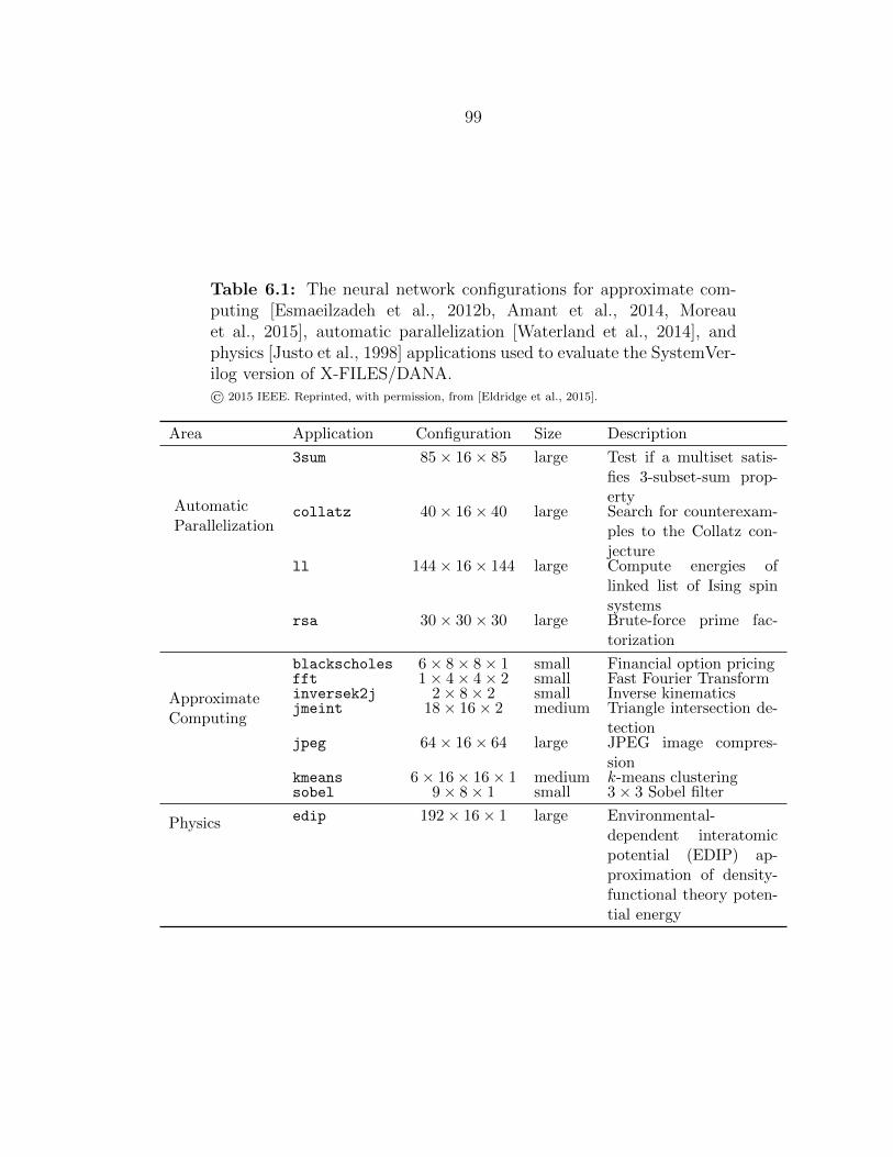
99
Table 6.1: The neural network configurations for approximate com-puting [Esmaeilzadeh et al., 2012b, Amant et al., 2014, Moreauet al., 2015], automatic parallelization [Waterland et al., 2014], andphysics [Justo et al., 1998] applications used to evaluate the SystemVer-ilog version of X-FILES/DANA.© 2015 IEEE. Reprinted, with permission, from [Eldridge et al., 2015].
Area Application Configuration Size Description
AutomaticParallelization
3sum 85× 16× 85 large Test if a multiset satis-fies 3-subset-sum prop-erty
collatz 40× 16× 40 large Search for counterexam-ples to the Collatz con-jecture
ll 144× 16× 144 large Compute energies oflinked list of Ising spinsystems
rsa 30× 30× 30 large Brute-force prime fac-torization
ApproximateComputing
blackscholes 6× 8× 8× 1 small Financial option pricingfft 1× 4× 4× 2 small Fast Fourier Transforminversek2j 2× 8× 2 small Inverse kinematicsjmeint 18× 16× 2 medium Triangle intersection de-
tectionjpeg 64× 16× 64 large JPEG image compres-
sionkmeans 6× 16× 16× 1 medium k-means clusteringsobel 9× 8× 1 small 3× 3 Sobel filter
Physics edip 192× 16× 1 large Environmental-dependent interatomicpotential (EDIP) ap-proximation of density-functional theory poten-tial energy
100
four neurons and each has one multiply accumulate to perform. Adding more PEs
beyond four cannot benefit the performance of this neural network in any way as the
neurons in the second hidden layer are waiting for the first hidden layer to finish.
This brings us to our second point, namely, that each of these neurons in the first
hidden layer only have a single multiply accumulate to perform. The limited amount
of work means that a PE allocated to the first hidden layer is not busy for very long
and increasing the number of elements per block has no effect. For these combined
reasons, we see the fft neural network demonstrate asymptotic behavior beyond four
PEs and identical behavior for both four and eight elements per block variations.
Relatedly, the design choice of fixed request bandwidth between PEs and storage
areas does, generally, render certain PE and block width configurations inefficient.
Specifically, when the number of PEs exceeds the elements per block, PEs are guar-
anteed to be waiting to access storage resources. This relates to the “amount of work”
argument above. A PE will generate a request to the Register File (or Scratchpad
Memories) and the Configuration Cache when it runs out of work to do, i.e., it runs
out of inputs and weights to process. Increasing the block size from four to eight
(or more) elements per block allows each request to grab more data and increase
the time between subsequent requests for more data by each PE. However, when the
block size is less than the number of PEs, the PEs are frequently waiting as they need
to arbitrate amongst themselves to determine who gets access to the Register File (or
Scratchpad Memories) and the Configuration Cache.
This behavior is most prominent for “large” neural networks with sufficient parallel
work (number of neurons in a layer) and sufficient work per neuron (the number of
neurons in the previous layer). The neural network for edip works as a good example.
We see edip show significant improvements when moving from four to eight elements
per block with gains approaching a theoretical 2×. Unfortunately, this strategy of

101
increasing the number of elements per block breaks down under two scenarios. First,
certain neural network configurations do not exhibit sufficient parallelism or work
per neuron, e.g., fft. This limitation, however, can be somewhat remedied by using
DANA’s capacity to execute multiple transactions simultaneously (see Section 6.2.2).
Second, increasing the block size requires increasing the bandwidth between modules.
Consequently, increasing the block size beyond a certain point becomes infeasible.
6.2.2 Single and multi-transaction throughput
We go on to evaluate the throughput of the X-FILES/DANA architecture for both
single and multi-transaction usage models. First, and using the same neural network
configurations shown in Table 6.1, we compute the throughput of X-FILES/DANA
when running a single transaction comprised of one feedforward inference. Figure 6·4
shows these results.
These results demonstrate some interacting effects related to how well the neurons
in a neural network “fit” into the number of available PEs. Take edip as an example
with its 192× 16× 1 topology. The amount of work each neuron in the hidden layer
has to do (192 multiplications) dwarfs the block size. Each allocated PE in the hidden
layer can then be viewed as being allocated for a long time. When the hidden layer
of 16 neurons aligns with some multiple of the number of PEs, then we see noticeable
jumps in the throughput. In effect, a six-PE configuration performs just as well as a
seven-PE configuration while an eight-PE configuration performs markedly better.
Generally, we view this as an opportunity for improving the throughput by ex-
posing multiple simultaneous transactions. The seven-PE configuration is obviously
leaving throughput on the table and, by providing additional work for the accelerator,
we can improve the scaling behavior as we add more PEs. Figure 6·5 shows the same
throughput plots but when running two simultaneous transactions. We select fft,
kmeans, and edip as these respectively represent small, medium, and large neural
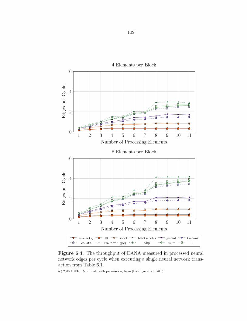
102
1 2 3 4 5 6 7 8 9 10 110
2
4
6
Number of Processing Elements
Edge
sp
erC
ycl
e4 Elements per Block
1 2 3 4 5 6 7 8 9 10 110
2
4
6
Number of Processing Elements
Edge
sp
erC
ycl
e
8 Elements per Block
inversek2j fft sobel blackscholes jmeint kmeans
collatz rsa jpeg edip 3sum ll
Figure 6·4: The throughput of DANA measured in processed neuralnetwork edges per cycle when executing a single neural network trans-action from Table 6.1.© 2015 IEEE. Reprinted, with permission, from [Eldridge et al., 2015].
103
network configurations for our motivating applications.
As an initial observation, the behavior is much more linear—the staircase behavior
of Figure 6·4 disappears once we expose multiple transactions to X-FILES/DANA.
Nevertheless, the absolute improvements are difficult to measure just by visually
comparing Figures 6·4 and 6·5.
Figure 6·6 shows the throughput speedup when running two neural network trans-
actions simultaneously versus serially. Overall, we see a maximum improvement of
30% with an average speedup of greater than 10%. Note that not all configurations
see this speedup. Specifically, two edip transactions show a significant decrease in
performance. This is an unfortunate artifact of the architecture of this SystemVer-
ilog implementation of X-FILES/DANA. The coordination between the Transaction
Table and the Control Module to allocate neurons to PEs, for this version, allocates
neurons in subsequent layers before the current layer finishes. When two instances of
edip, with their 16 hidden neurons per hidden layer, execute on DANA there exists
one optimal assignment pattern of neurons to PEs. Specifically, if the allocation of
PEs is in any way uneven, the single output neuron from one of the PEs will be allo-
cated before all of the neurons in its hidden layer finish. The large number of input
neurons, 192, exacerbates this problem and causes this PE with an output neuron to
sit idle for a long time. If the PEs are allocated perfectly, this problem does not occur.
However, any (likely) deviation in the start times of the transactions will result in a
suboptimal allocation procedure.
For this reason, the subsequent reimplementation of X-FILES/DANA in Chisel
does not allocate neurons in later layers until all neurons in the current layer have
completed execution. This does, however, leave some minimal performance on the
table for single transaction processing (PEs begin execution a few cycles faster if they
are preallocated before their inputs are ready). Nevertheless, our general view and
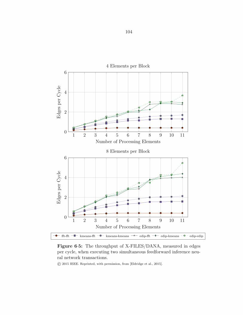
104
1 2 3 4 5 6 7 8 9 10 110
2
4
6
Number of Processing Elements
Edge
sp
erC
ycl
e
4 Elements per Block
1 2 3 4 5 6 7 8 9 10 110
2
4
6
Number of Processing Elements
Edge
sp
erC
ycl
e
8 Elements per Block
fft-fft kmeans-fft kmeans-kmeans edip-fft edip-kmeans edip-edip
Figure 6·5: The throughput of X-FILES/DANA, measured in edgesper cycle, when executing two simultaneous feedforward inference neu-ral network transactions.© 2015 IEEE. Reprinted, with permission, from [Eldridge et al., 2015].
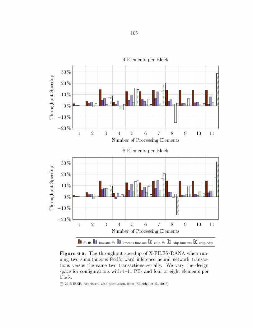
105
1 2 3 4 5 6 7 8 9 10 11−20 %
−10 %
0 %
10 %
20 %
30 %
Number of Processing Elements
Thro
ugh
put
Sp
eedup
4 Elements per Block
1 2 3 4 5 6 7 8 9 10 11−20 %
−10 %
0 %
10 %
20 %
30 %
Number of Processing Elements
Thro
ugh
put
Sp
eedup
8 Elements per Block
fft-fft kmeans-fft kmeans-kmeans edip-fft edip-kmeans edip-edip
Figure 6·6: The throughput speedup of X-FILES/DANA when run-ning two simultaneous feedforward inference neural network transac-tions versus the same two transactions serially. We vary the designspace for configurations with 1–11 PEs and four or eight elements perblock.© 2015 IEEE. Reprinted, with permission, from [Eldridge et al., 2015].

106
Table 6.2: Energy, delay, and energy delay product (EDP) reductionswhen executing neural network configurations on X-FILES/DANAcompared to a purely software implementation running on a gem5-simulated single core of an Intel Single Chip Cloud (SCC) system.Power evaluations were computed using McPAT [Li et al., 2009].© 2015 IEEE. Reprinted, with permission, from [Eldridge et al., 2015].
NN Energy Delay Energy–Delay Product
3sum 7× 95× 664×collatz 8× 106× 826×ll 6× 88× 569×rsa 6× 88× 566×
motivating applications demonstrate the need for multi-transaction systems and the
resulting multi-transaction throughput improvements, as demonstrated by Figure 6·6,
are significant.
As an additional evaluation of this implementation of X-FILES/DANA, we pro-
vide an energy and performance comparison against a software implementation. Our
software implementation uses the FANN library running on the gem5 system sim-
ulator acting as one core of an Intel Single Chip Cloud (SCC) microprocessor. We
estimate the power of the Intel SCC software-only version using McPAT [Li et al.,
2009]. The only software optimization used by FANN is software pipelining. Our
energy and delay comparison points for X-FILES/DANA are from our placed and
routed 40nm design. We assume that the neural network configurations are not avail-
able in DANA’s Configuration Cache and have to be loaded in over a multi-cycle
operation that loads one block per cycle.
Table 6.2 shows dramatic, though expected, improvements over this floating point
software implementation. Tangentially, we are generally skeptical of the overall ac-
curacy of this type of power modeling [Xi et al., 2015]. Nonetheless, a 2–3 order
of magnitude improvement over a software implementation for a dedicated piece of
hardware optimized for neural network processing is not unexpected.
For additional, automated testing, this X-FILES/DANA version was wrapped in
107
a UART interface and loaded onto a Xilinx Zynq FPGA. Error checking against a
floating point version of FANN validated the correctness of this SystemVerilog im-
plementation. Finally, this FPGA implementation was interfaced with the automatic
parallelization work of our collaborators to demonstrate an end-to-end system that
offloads neural network inferences to our dedicated X-FILES/DANA hardware.
6.3 Rocket + X-FILES/DANA
As a followup to this SystemVerilog version, we wanted to more tightly integrate
X-FILES/DANA with a RISC-V microprocessor.2 Using the lessons learned from the
SystemVerilog version (i.e., a Register File structure adds significant complexity and
aggressive PE allocation leads to subpar performance in multi-transaction scenarios),
we reimplemented X-FILES/DANA in the Chisel HDL [Bachrach et al., 2012]. We
previously described the resulting architecture in Chapters 4 and 5.
Following a vanilla port of SystemVerilog to Chisel and a conversion of the Register
File to per-transaction Scratchpad Memories, we added support for gradient descent
learning whose operation is discussed in Section 5.3.2. Learning support is, however,
an optional parameter, i.e., X-FILES/DANA can be built to either support or not
support learning.
Using the complete Rocket + X-FILES/DANA system we then evaluated the new
capabilities of this architecture on gradient descent learning tasks. Using different
neural networks provided by the FANN library and shown in Table 6.3, we executed
gradient descent learning3 on Rocket + X-FILES/DANA. Our only concern at this
2We chose RISC-V due to its completely open nature (anyone can design a RISC-V microprocessorwithout a license), our initial thought that we would need to implement changes to the underlyingISA to support X-FILES/DANA, and the existence and active development of implementations ofRISC-V microprocessors by others, e.g., UC Berkeley’s Rocket [UC Berkeley Architecture ResearchGroup, 2016].
3This is true gradient descent learning in that we do not use batching and compute the gradientof the entire training set before updating the weights of the neural network.
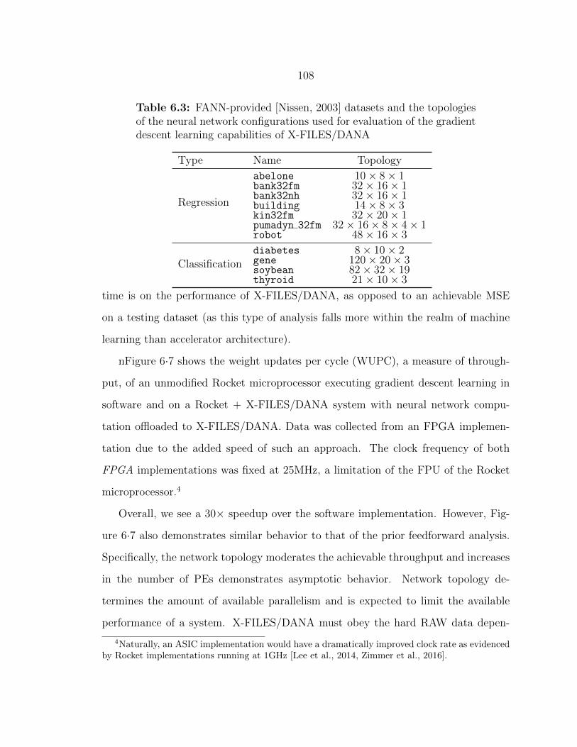
108
Table 6.3: FANN-provided [Nissen, 2003] datasets and the topologiesof the neural network configurations used for evaluation of the gradientdescent learning capabilities of X-FILES/DANA
Type Name Topology
Regression
abelone 10× 8× 1bank32fm 32× 16× 1bank32nh 32× 16× 1building 14× 8× 3kin32fm 32× 20× 1pumadyn 32fm 32× 16× 8× 4× 1robot 48× 16× 3
Classificationdiabetes 8× 10× 2gene 120× 20× 3soybean 82× 32× 19thyroid 21× 10× 3
time is on the performance of X-FILES/DANA, as opposed to an achievable MSE
on a testing dataset (as this type of analysis falls more within the realm of machine
learning than accelerator architecture).
nFigure 6·7 shows the weight updates per cycle (WUPC), a measure of through-
put, of an unmodified Rocket microprocessor executing gradient descent learning in
software and on a Rocket + X-FILES/DANA system with neural network compu-
tation offloaded to X-FILES/DANA. Data was collected from an FPGA implemen-
tation due to the added speed of such an approach. The clock frequency of both
FPGA implementations was fixed at 25MHz, a limitation of the FPU of the Rocket
microprocessor.4
Overall, we see a 30× speedup over the software implementation. However, Fig-
ure 6·7 also demonstrates similar behavior to that of the prior feedforward analysis.
Specifically, the network topology moderates the achievable throughput and increases
in the number of PEs demonstrates asymptotic behavior. Network topology de-
termines the amount of available parallelism and is expected to limit the available
performance of a system. X-FILES/DANA must obey the hard RAW data depen-
4Naturally, an ASIC implementation would have a dramatically improved clock rate as evidencedby Rocket implementations running at 1GHz [Lee et al., 2014, Zimmer et al., 2016].
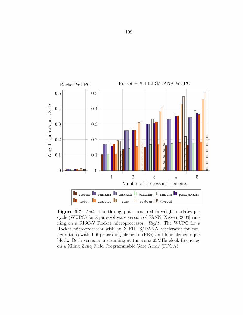
109
0
0.1
0.2
0.3
0.4
0.5
Wei
ght
Up
dat
esp
erC
ycl
e
Rocket WUPC
1 2 3 4 5
0
0.1
0.2
0.3
0.4
0.5
Number of Processing Elements
Rocket + X-FILES/DANA WUPC
abelone bank32fm bank32nh building kin32fm pumadyn-32fm
robot diabetes gene soybean thyroid
Figure 6·7: Left : The throughput, measured in weight updates percycle (WUPC) for a pure-software version of FANN [Nissen, 2003] run-ning on a RISC-V Rocket microprocessor. Right : The WUPC for aRocket microprocessor with an X-FILES/DANA accelerator for con-figurations with 1–6 processing elements (PEs) and four elements perblock. Both versions are running at the same 25MHz clock frequencyon a Xilinx Zynq Field Programmable Gate Array (FPGA).

110
dencies inherent in the structure of a neural network.5 Consequently, networks with
ample parallelism, like soybean, demonstrate the highest throughput while smaller
networks, like abelone, demonstrate reduced throughput. Allowing multiple trans-
actions to execute would, assumedly, improve the overall throughput in the same way
that multi-transaction operation improves the throughput of feedforward inference.
In regards to asymptotic behavior, the marginal benefit of increasing the number
of PEs eventually becomes negligible and would require an increase in the block size
to more fully take advantage of these PEs. Nonetheless, increasing the bandwidth
between components will eventually hit fundamental limits in the number of connect-
ing wires between modules. More sophisticated architectural improvements via new
X-FILES backends that avoid these bandwidth issues are discussed in Section 7.3.4.
6.4 Summary
We demonstrate the capabilities of the X-FILES/DANA neural network accelerator
for both feedforward inference and gradient descent learning applications. The small
neural network topologies used by some emerging application domains, approximate
computing and automatic parallelization, can be mitigated by exposing multiple si-
multaneous transactions (and, consequently, more parallel work) to X-FILES/DANA.
For further evaluation on the part of the reader, we provide X-FILES/DANA as
open source hardware on GitHub [Boston University Integrated Circuits and Systems
Group, 2016].
5Nevertheless, researchers at Microsoft have demonstrated that ignoring these data dependenciesin learning applications can dramatically improve performance and, counterintuitively, improve theoverall accuracy of a trained machine learning model [Chilimbi et al., 2014].
111
Chapter 7
Conclusion
With this work we present and evaluate a multi-transaction model of neural network
computation intended to meet the needs of future machine learning applications. In
this section we summarize these contributions and provide some commentary on the
limitations of our proposed system and directions for future work.
7.1 Summary of Contributions
We present two distinctly different neural network accelerator architectures. The first,
T-fnApprox, is a fixed-topology, fixed-weight accelerator used for the approximation
of mathematical functions in the GNU C Library. The entirely fixed nature of this
system allows for dramatic order of magnitude EDP improvements over software
implementations of the same functions. Nevertheless, we do admit that this fixed
property becomes problematic with the rapidly varying nature of machine learning
research—new topologies and architectures are produced daily.
In effect, and directly addressing our multi-transaction thesis, we present X-
FILES/DANA, a system-level view of neural network accelerators that supports a
multi-transaction model of neural network acceleration. With this work we introduce
the concept of a neural network transaction that encompasses all the operations of a
user process requesting and using an accelerator for a single inference or batch learn-
ing step. Moreover, X-FILES/DANA not only encompasses accelerator hardware, but
also user-level software and supervisor-level data structures and kernel modifications

112
to enable the use of a neural network accelerator like DANA in a safe manner. We
have additionally gone through numerous refactors of our X-FILES/DANA hardware
to ensure the complete separation of these hardware components. Namely, the X-
FILES Hardware Arbiter concerns itself only with the management of neural network
transactions while DANA provides multilayer perceptron neural network acceleration.
Our evaluation of X-FILES/DANA demonstrates order of magnitude improve-
ments over software neural network libraries. Additionally, we show that the multi-
transaction nature of this architecture improves the throughput of the DANA backend
by approximately 15% across a wide range of neural network topologies from existing
work. Furthermore, we provide an open source implementation of X-FILES/DANA
in the Chisel HDL as a drop-in RoCC accelerator for RISC-V microprocessors that
can be immediately used and evaluated in simulation and in FPGA hardware.
7.2 Limitations of X-FILES/DANA
Nevertheless, the X-FILES/DANA architecture does have some limitations which,
though partially discussed in previous sections, we summarize here. The multi-
transaction throughput benefit comes as a result of us exploiting periods of com-
putation when a single transaction has limited available parallelism. This can occur
from two possible sources. First, a neural network may just be a small neural network
and not have much intrinsic parallelism at any point during its execution on DANA.
Second a large neural network has limited parallelism at the end of a layer when
neurons in the next layer are waiting to be allocated.
In regards to the case of small neural networks, recent commentary from the ma-
chine learning community suggests that small neural networks are not useful and
should not even been considered—deep and wide neural networks are where all the
interesting applications lie. We do admit that the advances of deep learning are dra-
113
matic. However, we firmly believe in using an appropriately sized neural network for
the task. The work of Esmailzadeh [Esmaeilzadeh et al., 2012b] and Waterland [Wa-
terland et al., 2014] demonstrate the utility of small neural networks for useful tasks,
i.e., approximate computing and automatic parallelization, respectively. Addition-
ally, recent literature demonstrates that there are significant sources of inefficiency in
current deep learning models. Work on the compression of deep neural networks to
more compact representations [Han et al., 2015] and on heavy bit optimization and
trimming of neural networks [Reagen et al., 2016] bolsters this argument.
Related to the case of very large neural networks, our approach with the Chsiel
implementation of X-FILES/DANA where later layers wait for earlier layers to finish
may be overly conservative. A more apt approach would be to allow neurons from sub-
sequent layers to be allocated as long as they have sufficient work to keep them busy
and performing this allocation will not cause the limited performance degradations
of Figure 6·6. A more advanced PE allocation algorithm could deliver the perfor-
mance of our multi-transaction system with just a single transaction by allowing PEs
in subsequent layers to tentatively proceed with the data that is already available.
Alternatively, the work of Project Adam, previously mentioned, may indicate that
PEs can proceed blindly without waiting for data to be available [Chilimbi et al.,
2014]. For approximate computing applications, which are approximate to begin
with, introducing another source of approximation may, likely, be a safe performance
trade-off.
On the technical side, DANA is presently limited in that a neural network config-
uration must fit within the size of a single cache memory (approximately 32KB, or
the size of a unified L1 cache, at maximum). Larger configurations are not presently
supported. However, with modifications to the Configuration Cache and the ASID–
NNID Table Walker, weights can be streamed into the Configuration Cache as needed.
114
The regular, known access patterns of neural network weights facilitates this paging
process.
7.3 Future Work
There are substantial opportunities for this work to be furthered in addition to ex-
plorations related to mitigating the present limitations of X-FILES/DANA.
7.3.1 Transaction granularity
While we firmly believe that the concept of a neural network transaction has utility,
there are certain issues with its definition. Specifically, the amount of computation
required for a neural network transaction, currently defined as encompassing all the
operations of a feedforward inference or a single stochastic gradient descent update
over some batch size, is dependent on neural network topology. Put simply, small
networks have less computation than big networks. This variability in the “size” of
a transaction makes scheduling difficult and provides motivation for breaking down
transactions into more finely-grained steps. Within the scope of DANA, this involves
converting each neural network transaction into a set of assignments to PEs. At a
very high level, DANA can be viewed as dynamically translating a neural network
transaction into a sequence of microcoded address computations, transaction state
updates, and PE assignment operations.
While acceptable, a cleaner (and more RISC-like) approach involves defining neu-
ral network transactions as the elementary instructions of neural network computa-
tion. The question then becomes, “What are the fundamental units of neural network
computation?” Within the scope of this work, these should necessarily include vector–
vector multiplication representing the input–weight products of all-to-all connected
MLP neurons, backpropagation instructions supporting stochastic gradient descent,
and weight update instructions the can be used to construct stochastic or batched

115
modifications of NN connections. In light of recent interest in CNNs and other DNNs,
these should additionally include convolution with a fixed kernel and stride and max-
pooling/averaging over a window with a specific stride.
7.3.2 Variable transaction priority
Alternatively, allowing for variability in the priorities of existing neural network trans-
actions may mitigate some of the issues addressed above with transaction granularity.
At present, all transactions in X-FILES and DANA are arbitrated amongst using
round robin scheduling. In one sense, this is fair in that all transactions have an
equal opportunity to access hardware resources. However, this is not always ideal.
Specifically, transactions involving large neural network configurations may initially
monopolize all the available PEs and prevent a second transaction with a small neural
network from beginning execution. Relatedly, an optimal decision may be to weight
the arbitration based on the amount of work that a transaction has to perform. These
questions remain open and warrant further investigation.
In a more concrete comment and related to the notion of X-FILES as providing
access to hardware-backed learning and inference for all user and supervisor processes,
a standard notion of process niceness should likely be observed. In our view, the
operating system could utilize a neural network accelerator to make a quick decision
on some difficult to program task, e.g., cache prefetching. However, operating system
operations must be fast. The operating system cannot afford to have DANA tied
up with a long running learning transaction that could run overnight. The normal
operating system concept of process niceness could be utilized to make it safer for the
operating system to use a hardware accelerator like DANA by either putting some
hard bound on the latency of a transaction or ensuring that a transaction will proceed
as fast as possible.

116
7.3.3 Asynchronous in-memory input–output queues
The asynchronous input–output queues of the ASID–NNID Table described in Sec-
tion 4.2.2 and shown in Figure 4·4 are not currently implemented. All communication
related to transaction initiation and input or output data transfer occur through the
command/response portion of the RoCC interface. The implementation and use of an
asynchronous in-memory interface requires further exploration. Specifically, the use
of a completely asynchronous interface allows X-FILES/DANA to do its own flow con-
trol independent of the command/response interface. Relatedly, this then naturally
allows one accelerator to operate on transactions from any core in the system. An
early version of X-FILES/DANA supported a parameterized number of RoCC connec-
tions to support acceleration of incident transactions from multiple cores. However,
this adds a substantial amount of overhead as all input lines need to be buffered and
undergo arbitration. This complexity can be avoided with the use of these in-memory
queues.
Nevertheless, for a proper implementation, X-FILES/DANA would need to par-
ticipate in the cache coherency protocol in a way different from what is currently
provided by the RoCC interface. Specifically, both the L1 and L2 interfaces that the
RoCC interface provides do not allow for explicit use of Tilelink 1 probes that would
act as doorbells telling X-FILES/DANA that new data is available. Alternatively, and
naively, X-FILES/DANA would need to actively poll specific memory regions to look
for new transaction packets to process. This is both inefficient from the perspective
of X-FILES/DANA and can wreak havoc to the caches. Broadly, modifications to the
existing ASID–NNID Table require investigation for ways to improve the asynchronicity
of X-FILES backends.
1Tilelink is a protocol-agnostic implementation of a cache coherency substrate.
117
7.3.4 New X-FILES backends
While we present and discuss the architecture of DANA at length, DANA is only
one possible X-FILES backend. Our design of X-FILES user and supervisor software,
supervisor data structures, and the X-FILES Hardware Arbiter were all done to ensure
that new machine learning accelerators could benefit from all the existing X-FILES
infrastructure. The limitations of DANA, as outlined in Section 7.2, can be largely
remedied with a new architecture that allows for explicit communication between
PEs. Direct PE to PE communication improves the efficiency of the system, provides
a more natural architecture, and, critically, removes the Scratchpad Memories as
bottlenecks for communication. A generic architecture improving DANA in this way
would likely be of either dataflow or systolic array varieties.
Alternatively, and addressing criticism of MLP neural network accelerators, new
backends for more topical neural network flavors can be developed. These include, but
are not limited to, Convolutional Neural Networks, Recurrent Neural Networks (in-
cluding LSTM), and Deep Belief Networks (stacked Restricted Boltzmann Machines).
Nevertheless, the use of these new backends requires substantial rearchitecting of the
Configuration Cache and the PEs. The Configuration Cache needs to support larger
neural network configurations on the order of tens to hundreds of megabytes. The
notion of caching these configurations locally becomes nonsensical due to existing
memory technologies (though advances in 3D stacking and nonvolatile memory tech-
nologies may provide direct ways forward). Hence, the Configuration Cache begins to
look much more like a direct memory access unit optimized for reading neural network
configurations. The PEs would need to be modified, in addition to dataflow/systolic
array architectures, to support new types of operations and activation functions. Ar-
guably, the PEs should be highly programmable to align with whatever new flavor of
neural network becomes popular in the machine learning community.
118
7.3.5 Linux kernel modifications
Modifications to the Linux kernel to support the X-FILES are in progress and will be
made available publicly once completed. More generally, operating system support for
accelerators tightly coupled with a microprocessor and having access to the memory
hierarchy is likely needed. The breakdown of Dennard scaling and the tapering off
of Moore’s Law have resulted in the modern area of computer engineering being
christened the “Golden Age of Architecture.” Consequently, there exist numerous
opportunities for systems directly interacting with the hardware (the operating system
and its device drivers) to evolve simultaneously.
7.4 Final Remarks
In summary, we propose, implement, and validate a multi-transaction model of neural
network computation and acceleration and make our work available to the community.
With this work we have necessarily taken and applied a holistic, system level view,
encompassing hardware design as well as user and supervisor software development
to neural network computation. It is our firm belief that advances in the field of
electrical and computer engineering are increasingly requiring such a broad base of
knowledge and collaboration across departments and specialties.

119
References
[Abadi et al., 2015] Abadi, M., Agarwal, A., Barham, P., Brevdo, E., Chen, Z., Citro,C., Corrado, G. S., Davis, A., Dean, J., Devin, M., Ghemawat, S., Goodfellow,I., Harp, A., Irving, G., Isard, M., Jia, Y., Jozefowicz, R., Kaiser, L., Kudlur, M.,Levenberg, J., Mane, D., Monga, R., Moore, S., Murray, D., Olah, C., Schuster,M., Shlens, J., Steiner, B., Sutskever, I., Talwar, K., Tucker, P., Vanhoucke, V.,Vasudevan, V., Viegas, F., Vinyals, O., Warden, P., Wattenberg, M., Wicke, M.,Yu, Y., and Zheng, X. (2015). TensorFlow: Large-scale machine learning onheterogeneous systems. Software available from tensorflow.org.
[Agarwal et al., 2009] Agarwal, A., Rinard, M., Sidiroglou, S., Misailovic, S., andHoffmann, H. (2009). Using code perforation to improve performance, reduceenergy consumption, and respond to failures. Technical Report MIT-CSAIL-TR-2009-042, Massachusetts Institute of Technology.
[Al-Rfou et al., 2016] Al-Rfou, R., Alain, G., Almahairi, A., Angermueller, C., Bah-danau, D., Ballas, N., Bastien, F., Bayer, J., Belikov, A., Belopolsky, A., Bengio,Y., Bergeron, A., Bergstra, J., Bisson, V., Bleecher Snyder, J., Bouchard, N.,Boulanger-Lewandowski, N., Bouthillier, X., de Brebisson, A., Breuleux, O.,Carrier, P.-L., Cho, K., Chorowski, J., Christiano, P., Cooijmans, T., Cote,M.-A., Cote, M., Courville, A., Dauphin, Y. N., Delalleau, O., Demouth, J.,Desjardins, G., Dieleman, S., Dinh, L., Ducoffe, M., Dumoulin, V., EbrahimiKahou, S., Erhan, D., Fan, Z., Firat, O., Germain, M., Glorot, X., Goodfellow,I., Graham, M., Gulcehre, C., Hamel, P., Harlouchet, I., Heng, J.-P., Hidasi,B., Honari, S., Jain, A., Jean, S., Jia, K., Korobov, M., Kulkarni, V., Lamb,A., Lamblin, P., Larsen, E., Laurent, C., Lee, S., Lefrancois, S., Lemieux, S.,Leonard, N., Lin, Z., Livezey, J. A., Lorenz, C., Lowin, J., Ma, Q., Manzagol,P.-A., Mastropietro, O., McGibbon, R. T., Memisevic, R., van Merrienboer, B.,Michalski, V., Mirza, M., Orlandi, A., Pal, C., Pascanu, R., Pezeshki, M., Raffel,C., Renshaw, D., Rocklin, M., Romero, A., Roth, M., Sadowski, P., Salvatier, J.,Savard, F., Schluter, J., Schulman, J., Schwartz, G., Serban, I. V., Serdyuk, D.,Shabanian, S., Simon, E., Spieckermann, S., Subramanyam, S. R., Sygnowski,J., Tanguay, J., van Tulder, G., Turian, J., Urban, S., Vincent, P., Visin, F.,de Vries, H., Warde-Farley, D., Webb, D. J., Willson, M., Xu, K., Xue, L., Yao,L., Zhang, S., and Zhang, Y. (2016). Theano: A Python framework for fastcomputation of mathematical expressions. arXiv e-prints, abs/1605.02688.
[Amant et al., 2014] Amant, R. S., Yazdanbakhsh, A., Park, J., Thwaites, B., Es-

120
maeilzadeh, H., Hassibi, A., Ceze, L., and Burger, D. (2014). General-purposecode acceleration with limited-precision analog computation. In ACM/IEEE41st International Symposium on Computer Architecture, ISCA 2014, Minneapo-lis, MN, USA, June 14-18, 2014, pages 505–516.
[Asanovic et al., 1992] Asanovic, K., Beck, J., Kingsbury, B. E. D., Kohn, P., Mor-gan, N., and Wawrzynek, J. (1992). Spert: a vliw/simd microprocessor forartificial neural network computations. In In Proceedings of the InternationalConference on Application Specific Array Processors, 1992., pages 178–190.
[Bachrach et al., 2012] Bachrach, J., Vo, H., Richards, B., Lee, Y., Waterman, A.,Avizienis, R., Wawrzynek, J., and Asanovic, K. (2012). Chisel: Constructinghardware in a scala embedded language. In 49th ACM/EDAC/IEEE DesignAutomation Conference (DAC), 2012, pages 1212–1221.
[Bengio, 2009] Bengio, Y. (2009). Learning deep architectures for AI. Foundationsand Trends in Machine Learning, 2(1):1–127.
[Bienia, 2011] Bienia, C. (2011). Benchmarking Modern Multiprocessors. PhD thesis,Princeton University.
[Binkert et al., 2011] Binkert, N., Beckmann, B., Black, G., Reinhardt, S. K., Saidi,A., Basu, A., Hestness, J., Hower, D. R., Krishna, T., Sardashti, S., Sen, R.,Sewell, K., Shoaib, M., Vaish, N., Hill, M. D., and Wood, D. A. (2011). Thegem5 simulator. SIGARCH Computer Architecture News, 39(2):1–7.
[Boston University Integrated Circuits and Systems Group, 2016] Boston UniversityIntegrated Circuits and Systems Group (2016). X-files/dana github repository.Online: https://github.com/bu-icsg/xfiles-dana.
[Carbin et al., 2012] Carbin, M., Kim, D., Misailovic, S., and Rinard, M. C. (2012).Proving acceptability properties of relaxed nondeterministic approximate pro-grams. In Proceedings of the 33rd ACM SIGPLAN Conference on ProgrammingLanguage Design and Implementation, PLDI ’12, pages 169–180, New York, NY,USA. ACM.
[Carbin et al., 2013] Carbin, M., Kim, D., Misailovic, S., and Rinard, M. C. (2013).Verified integrity properties for safe approximate program transformations. InProceedings of the ACM SIGPLAN 2013 Workshop on Partial Evaluation andProgram Manipulation, PEPM ’13, pages 63–66, New York, NY, USA. ACM.
[Chen et al., 2012] Chen, T., Chen, Y., Duranton, M., Guo, Q., Hashmi, A., Lipasti,M., Nere, A., Qiu, S., Sebag, M., and Temam, O. (2012). Benchnn: On thebroad potential application scope of hardware neural network accelerators. InIEEE International Symposium on Workload Characterization (IISWC), pages36–45.
[Chen et al., 2014a] Chen, T., Du, Z., Sun, N., Wang, J., Wu, C., Chen, Y., andTemam, O. (2014a). Diannao: a small-footprint high-throughput accelerator

121
for ubiquitous machine-learning. In Architectural Support for ProgrammingLanguages and Operating Systems, ASPLOS ’14, Salt Lake City, UT, USA,March 1-5, 2014, pages 269–284.
[Chen et al., 2014b] Chen, Y., Luo, T., Liu, S., Zhang, S., He, L., Wang, J., Li, L.,Chen, T., Xu, Z., Sun, N., and Temam, O. (2014b). Dadiannao: A machine-learning supercomputer. In 47th Annual IEEE/ACM International Symposiumon Microarchitecture, MICRO 2014, Cambridge, United Kingdom, December 13-17, 2014, pages 609–622.
[Chetlur et al., 2014] Chetlur, S., Woolley, C., Vandermersch, P., Cohen, J., Tran, J.,Catanzaro, B., and Shelhamer, E. (2014). cudnn: Efficient primitives for deeplearning. CoRR, abs/1410.0759.
[Chilimbi et al., 2014] Chilimbi, T. M., Suzue, Y., Apacible, J., and Kalyanaraman,K. (2014). Project adam: Building an efficient and scalable deep learningtraining system. In 11th USENIX Symposium on Operating Systems Designand Implementation, OSDI ’14, Broomfield, CO, USA, October 6-8, 2014., pages571–582.
[Chippa et al., 2013] Chippa, V. K., Chakradhar, S. T., Roy, K., and Raghunathan,A. (2013). Analysis and characterization of inherent application resilience forapproximate computing. In The 50th Annual Design Automation Conference2013, DAC ’13, Austin, TX, USA, May 29 - June 07, 2013, pages 113:1–113:9.
[Cobham, 1965] Cobham, A. (1965). The intrinsic computational difficulty of func-tions. In Bar-Hillel, Y., editor, Logic, Methodology and Philosophy of Science:Proceedings of the 1964 International Congress (Studies in Logic and the Foun-dations of Mathematics), pages 24–30. North-Holland Publishing.
[Collobert et al., ] Collobert, R., Kavukcuoglu, K., and Farabet, C. Torch7:A matlab-like environment for machine learning. Available from:http://publications.idiap.ch/downloads/papers/2011/Collobert_
NIPSWORKSHOP_2011.pdf.
[Cybenko, 1989] Cybenko, G. (1989). Approximation by superpositions of a sig-moidal function. Mathematics of Control, Signals and Systems, 2(4):303–314.
[Deng et al., 2009] Deng, J., Dong, W., Socher, R., Li, L.-J., Li, K., and Fei-Fei, L.(2009). ImageNet: A Large-Scale Hierarchical Image Database. In ComputerVision and Pattern Recognition.
[Dreyfus, 1965] Dreyfus, H. L. (1965). Alchemy and artificial intelligence. RANDPaper P-3244. Santa Monica, CA: Rand Corp.
[Eldridge et al., 2014] Eldridge, S., Raudies, F., Zou, D., and Joshi, A. (2014). Neu-ral network-based accelerators for transcendental function approximation. InGreat Lakes Symposium on VLSI 2014, GLSVLSI ’14, Houston, TX, USA -May 21 - 23, 2014, pages 169–174.
122
[Eldridge et al., 2015] Eldridge, S., Waterland, A., Seltzer, M., Appavoo, J., andJoshi, A. (2015). Towards general-purpose neural network computing. In 2015International Conference on Parallel Architecture and Compilation, PACT 2015,San Francisco, CA, USA, October 18-21, 2015, pages 99–112.
[Esmaeilzadeh et al., 2012a] Esmaeilzadeh, H., Sampson, A., Ceze, L., and Burger,D. (2012a). Architecture support for disciplined approximate programming. InProceedings of the 17th International Conference on Architectural Support forProgramming Languages and Operating Systems, ASPLOS 2012, London, UK,March 3-7, 2012, pages 301–312.
[Esmaeilzadeh et al., 2012b] Esmaeilzadeh, H., Sampson, A., Ceze, L., and Burger,D. (2012b). Neural acceleration for general-purpose approximate programs. In45th Annual IEEE/ACM International Symposium on Microarchitecture, MI-CRO 2012, Vancouver, BC, Canada, December 1-5, 2012, pages 449–460.
[Fakhraie and Smith, 1997] Fakhraie, S. M. and Smith, K. C. (1997). VLSI Compat-ible Implementations for Artificial Neural Networks. Springer.
[Farabet et al., 2013] Farabet, C., Couprie, C., Najman, L., and LeCun, Y. (2013).Learning hierarchical features for scene labeling. IEEE Transactions on PatternAnalysis and Machine Intelligence, 35(8):1915–1929.
[Fleming, 1953] Fleming, I. (1953). Casino Royale. Jonathan Cape, London, UK.
[Fukushima, 1980] Fukushima, K. (1980). Neocognitron: A self-organizing neuralnetwork model for a mechanism of pattern recognition unaffected by shift inposition. Biological Cybernetics, 36(4):193–202.
[Graves et al., 2014] Graves, A., Wayne, G., and Danihelka, I. (2014). Neural turingmachines. CoRR, abs/1410.5401.
[Grigorian et al., 2015] Grigorian, B., Farahpour, N., and Reinman, G. (2015).BRAINIAC: bringing reliable accuracy into neurally-implemented approximatecomputing. In 21st IEEE International Symposium on High Performance Com-puter Architecture, HPCA 2015, Burlingame, CA, USA, February 7-11, 2015,pages 615–626.
[Grigorian and Reinman, 2014] Grigorian, B. and Reinman, G. (2014). Improvingcoverage and reliability in approximate computing using application-specific,light-weight checks. In 1st Workshop on Approximate Computing Across theSystem Stack.
[Han et al., 2015] Han, S., Mao, H., and Dally, W. J. (2015). Deep compression:Compressing deep neural network with pruning, trained quantization and huff-man coding. CoRR, abs/1510.00149.
[Hemingway, 1926] Hemingway, E. (1926). The Sun Also Rises. Scribner’s, NewYork City, New York.

123
[Hinton et al., 2006] Hinton, G. E., Osindero, S., and Teh, Y. W. (2006). A fastlearning algorithm for deep belief nets. Neural Computation, 18(7):1527–1554.
[Hochreiter and Schmidhuber, 1997] Hochreiter, S. and Schmidhuber, J. (1997).Long short-term memory. Neural Computation, 9(8):1735–1780.
[Hornik, 1991] Hornik, K. (1991). Approximation capabilities of multilayer feedfor-ward networks. Neural Networks, 4(2):251–257.
[Hubel and Wiesel, 1965] Hubel, D. H. and Wiesel, T. N. (1965). Receptive fieldsand functional architecture in two nonstriate visual areas (18 and 19) of the cat.Journal of Neurophysiology, 28:229–289.
[Jia et al., 2014] Jia, Y., Shelhamer, E., Donahue, J., Karayev, S., Long, J., Girshick,R. B., Guadarrama, S., and Darrell, T. (2014). Caffe: Convolutional architecturefor fast feature embedding. In Proceedings of the ACM International Conferenceon Multimedia, MM ’14, Orlando, FL, USA, November 03 - 07, 2014, pages675–678.
[Jonas and Kording, 2016] Jonas, E. and Kording, K. (2016). Could a neuroscientistunderstand a microprocessor? bioRxiv.
[Justo et al., 1998] Justo, J. a. F., Bazant, M. Z., Kaxiras, E., Bulatov, V. V., andYip, S. (1998). Interatomic potential for silicon defects and disordered phases.Physical Review B, 58:2539–2550.
[Kahng and Kang, 2012] Kahng, A. B. and Kang, S. (2012). Accuracy-configurableadder for approximate arithmetic designs. In The 49th Annual Design Automa-tion Conference 2012, DAC ’12, San Francisco, CA, USA, June 3-7, 2012, pages820–825.
[Kestur et al., 2012] Kestur, S., Park, M. S., Sabarad, J., Dantara, D., Narayanan,V., Chen, Y., and Khosla, D. (2012). Emulating mammalian vision on recon-figurable hardware. In 2012 IEEE 20th Annual International Symposium onField-Programmable Custom Computing Machines, FCCM 2012, 29 April - 1May 2012, Toronto, Ontario, Canada, pages 141–148.
[Khan et al., 2008] Khan, M. M., Lester, D. R., Plana, L. A., Rast, A. D., Jin, X.,Painkras, E., and Furber, S. B. (2008). Spinnaker: Mapping neural networksonto a massively-parallel chip multiprocessor. In Proceedings of the InternationalJoint Conference on Neural Networks, IJCNN 2008, part of the IEEE WorldCongress on Computational Intelligence, WCCI 2008, Hong Kong, China, June1-6, 2008, pages 2849–2856.
[Lazebnik, 2004] Lazebnik, Y. (2004). Can a biologist fix a radio? — or, what ilearned while studying apoptosis. Biochemistry (Moscow), 69(12):1403–1406.
[Lecun et al., 1998] Lecun, Y., Bottou, L., Bengio, Y., and Haffner, P. (1998).Gradient-based learning applied to document recognition. Proceedings of theIEEE, 86(11):2278–2324.
124
[Lee et al., 2014] Lee, Y., Waterman, A., Avizienis, R., Cook, H., Sun, C., Stojanovic,V., and Asanovic, K. (2014). A 45nm 1.3ghz 16.7 double-precision gflops/wrisc-v processor with vector accelerators. In 40th European Solid State CircuitsConference (ESSCIRC), pages 199–202.
[Li et al., 2009] Li, S., Ahn, J. H., Strong, R. D., Brockman, J. B., Tullsen, D. M.,and Jouppi, N. P. (2009). Mcpat: an integrated power, area, and timing mod-eling framework for multicore and manycore architectures. In 42nd AnnualIEEE/ACM International Symposium on Microarchitecture (MICRO-42 2009),December 12-16, 2009, New York, New York, USA, pages 469–480.
[Lighthill, 1973] Lighthill, J. (1973). Artificial intelligence: A general survey. InArtificial Intelligence: A Paper Symposium. London: Science Research Council.
[Liu et al., 2015] Liu, D., Chen, T., Liu, S., Zhou, J., Zhou, S., Teman, O., Feng,X., Zhou, X., and Chen, Y. (2015). Pudiannao: A polyvalent machine learningaccelerator. In Proceedings of the Twentieth International Conference on Ar-chitectural Support for Programming Languages and Operating Systems, pages369–381. ACM.
[Mahajan et al., 2016] Mahajan, D., Park, J., Amaro, E., Sharma, H., Yazdan-bakhsh, A., Kim, J. K., and Esmaeilzadeh, H. (2016). TABLA: A unifiedtemplate-based framework for accelerating statistical machine learning. In 2016IEEE International Symposium on High Performance Computer Architecture,HPCA 2016, Barcelona, Spain, March 12-16, 2016, pages 14–26.
[Markoff, t B1] Markoff, J. (2014, August 8, Sect B1). Ibm develops a new chip thatfunctions like a brain. The New York Times.
[McCulloch and Pitts, 1943] McCulloch, W. S. and Pitts, W. (1943). A logical cal-culus of the ideas immanent in nervous activity. The bulletin of mathematicalbiophysics, 5(4):115–133.
[Michie, 1968] Michie, D. (1968). Memo functions and machine learning. Nature,218(5136):19–22.
[Minsky and Papert, 1987] Minsky, M. and Papert, S. (1987). Perceptrons - anintroduction to computational geometry. MIT Press.
[Moreau et al., 2015] Moreau, T., Wyse, M., Nelson, J., Sampson, A., Esmaeilzadeh,H., Ceze, L., and Oskin, M. (2015). SNNAP: approximate computing on pro-grammable socs via neural acceleration. In 21st IEEE International Symposiumon High Performance Computer Architecture, HPCA 2015, Burlingame, CA,USA, February 7-11, 2015, pages 603–614.
[Morgan et al., 1990] Morgan, N., Beck, J., Kohn, P., Bilmes, J., Allman, E., andBeer, J. (1990). The rap: a ring array processor for layered network calculations.In Proceedings of the International Conference on Application Specific ArrayProcessors, 1990., pages 296–308.
125
[Morgan et al., 1992] Morgan, N., Beck, J., Kohn, P., Bilmes, J., Allman, E., andBeer, J. (1992). The ring array processor: A multiprocessing peripheral forconnectionist applications. Journal of Parallel and Distributed Computing,14(3):248–259.
[Nissen, 2003] Nissen, S. (2003). Implementation of a fast artificial neural networklibrary (fann). Technical report, Department of Computer Science University ofCopenhagen (DIKU). http://fann.sf.net.
[Preissl et al., 2012] Preissl, R., Wong, T. M., Datta, P., Flickner, M., Singh, R.,Esser, S. K., Risk, W. P., Simon, H. D., and Modha, D. S. (2012). Compass: ascalable simulator for an architecture for cognitive computing. In SC Conferenceon High Performance Computing Networking, Storage and Analysis, SC ’12, SaltLake City, UT, USA - November 11 - 15, 2012, page 54.
[Przytula, 1991] Przytula, K. W. (1991). Parallel digital implementations of neuralnetworks. In Proceedings of the International Conference on Application SpecificArray Processors, 1991, pages 162–176.
[Raudies et al., 2014] Raudies, F., Eldridge, S., Joshi, A., and Versace, M. (2014).Learning to navigate in a virtual world using optic flow and stereo disparitysignals. Artificial Life and Robotics, 19(2):157–169.
[Reagen et al., 2016] Reagen, B., Whatmough, P. N., Adolf, R., Rama, S., Lee, H.,Lee, S. K., Hernandez-Lobato, J. M., Wei, G., and Brooks, D. M. (2016). Min-erva: Enabling low-power, highly-accurate deep neural network accelerators. In43rd ACM/IEEE Annual International Symposium on Computer Architecture,ISCA 2016, Seoul, South Korea, June 18-22, 2016, pages 267–278.
[Rinard, 2007] Rinard, M. C. (2007). Using early phase termination to eliminateload imbalances at barrier synchronization points. In Proceedings of the 22ndAnnual ACM SIGPLAN Conference on Object-Oriented Programming, Systems,Languages, and Applications, OOPSLA 2007, October 21-25, 2007, Montreal,Quebec, Canada, pages 369–386.
[RISC-V Foundation, 2016a] RISC-V Foundation (2016a). Risc-v port of the linuxkernel. Online: https://github.com/riscv/riscv-linux.
[RISC-V Foundation, 2016b] RISC-V Foundation (2016b). Risc-v proxy kernelgithub repository. Online: https://github.com/riscv/riscv-pk.
[Rosenblatt, 1958] Rosenblatt, F. (1958). The perceptron: a probabilistic modelfor information storage and organization in the brain. Psycholigcal Review,65(6):386.
[Rumelhart et al., 1988] Rumelhart, D. E., Hinton, G. E., and Williams, R. J. (1988).Learning representations by back-propagating errors. Cognitive modeling, 5(3):1.
[Sampson et al., 2011] Sampson, A., Dietl, W., Fortuna, E., Gnanapragasam, D.,Ceze, L., and Grossman, D. (2011). Enerj: approximate data types for safe and
126
general low-power computation. In Proceedings of the 32nd ACM SIGPLANConference on Programming Language Design and Implementation, PLDI 2011,San Jose, CA, USA, June 4-8, 2011, pages 164–174.
[Sampson et al., 2013] Sampson, A., Nelson, J., Strauss, K., and Ceze, L. (2013).Approximate storage in solid-state memories. In The 46th Annual IEEE/ACMInternational Symposium on Microarchitecture, MICRO-46, Davis, CA, USA,December 7-11, 2013, pages 25–36.
[Savich et al., 2007] Savich, A. W., Moussa, M., and Areibi, S. (2007). The impact ofarithmetic representation on implementing MLP-BP on fpgas: A study. IEEETransactions on Neural Networks, 18(1):240–252.
[Shannon, 1938] Shannon, C. E. (1938). A symbolic analysis of relay and switch-ing circuits. Transactions of the American Institute of Electrical Engineers,57(12):713–723.
[Sharma et al., 2016] Sharma, H., Park, J., Amaro, E., Thwaites, B., Kotha, P.,Gupta, A., Kim, J. K., Mishra, A., and Esmaeilzadeh, H. (2016). Dnnweaver:From high-level deep network models to fpga acceleration. In the Workshop onCognitive Architectures.
[Shivakumar and Jouppi, 2001] Shivakumar, P. and Jouppi, N. P. (2001). Cacti 3.0:An integrated cache timing, power, and area model. Technical Report 2001/2,Compaq Computer Corporation.
[Sidiroglou-Douskos et al., 2011] Sidiroglou-Douskos, S., Misailovic, S., Hoffmann,H., and Rinard, M. C. (2011). Managing performance vs. accuracy trade-offswith loop perforation. In SIGSOFT/FSE’11 19th ACM SIGSOFT Symposiumon the Foundations of Software Engineering (FSE-19) and ESEC’11: 13th Euro-pean Software Engineering Conference (ESEC-13), Szeged, Hungary, September5-9, 2011, pages 124–134.
[Siegelmann and Sontag, 1995] Siegelmann, H. T. and Sontag, E. D. (1995). On thecomputational power of neural nets. Journal of Computer System Sciences,50(1):132–150.
[Stine et al., 2007] Stine, J. E., Castellanos, I. D., Wood, M. H., Henson, J., Love,F., Davis, W. R., Franzon, P. D., Bucher, M., Basavarajaiah, S., Oh, J., andJenkal, R. (2007). Freepdk: An open-source variation-aware design kit. In IEEEInternational Conference on Microelectronic Systems Education, MSE ’07, SanDiego, CA, USA, June 3-4, 2007, pages 173–174.
[The Cure, 1980] The Cure (1980). A forest. Seventeen Seconds.
[The Cure, 1985] The Cure (1985). Push. The Head On The Door.
[Turing, 1950] Turing, A. M. (1950). Computing machinery and intelligence. Mind,59(236):433–460.
127
[UC Berkeley Architecture Research Group, 2016] UC Berkeley Architecture Re-search Group (2016). Rocket chip github repository. Online: https:
//github.com/ucb-bar/rocket-chip.
[Venkataramani et al., 2013] Venkataramani, S., Chippa, V. K., Chakradhar, S. T.,Roy, K., and Raghunathan, A. (2013). Quality programmable vector processorsfor approximate computing. In The 46th Annual IEEE/ACM InternationalSymposium on Microarchitecture, MICRO-46, Davis, CA, USA, December 7-11,2013, pages 1–12.
[Venkatesh et al., 2010] Venkatesh, G., Sampson, J., Goulding, N., Garcia, S.,Bryksin, V., Lugo-Martinez, J., Swanson, S., and Taylor, M. B. (2010). Conser-vation cores: reducing the energy of mature computations. In Proceedings of the15th International Conference on Architectural Support for Programming Lan-guages and Operating Systems, ASPLOS 2010, Pittsburgh, Pennsylvania, USA,March 13-17, 2010, pages 205–218.
[Vo et al., 2013] Vo, H., Lee, Y., Waterman, A., and Asanovic, K. (2013). A casefor os-friendly hardware accelerators. In Workshop on the Interaction BetweenOperating System and Computer Architecture.
[Volder, 1959] Volder, J. E. (1959). The CORDIC trigonometric computing tech-nique. IRE Transactions on Electronic Computers, 8(3):330–334.
[von Neumann, 1956] von Neumann, J. (1956). Probabilistic logics and the synthesisof reliable organisms from unreliable components. Automata studies, 34:43–98.
[von Neumann, 1993] von Neumann, J. (1993). First draft of a report on the edvac.IEEE Annals of the History of Computing, 15(4):27–75.
[Walther, 1971] Walther, J. S. (1971). A unified algorithm for elementary functions.In American Federation of Information Processing Societies: AFIPS ConferenceProceedings: 1971 Spring Joint Computer Conference, Atlantic City, NJ, USA,May 18-20, 1971, pages 379–385.
[Waterland et al., 2014] Waterland, A., Angelino, E., Adams, R. P., Appavoo, J., andSeltzer, M. I. (2014). ASC: automatically scalable computation. In ArchitecturalSupport for Programming Languages and Operating Systems, ASPLOS ’14, SaltLake City, UT, USA, March 1-5, 2014, pages 575–590.
[Waterland et al., 2012] Waterland, A., Appavoo, J., and Seltzer, M. (2012). Paral-lelization by simulated tunneling. In 4th USENIX Workshop on Hot Topics inParallelism, HotPar’12, Berkeley, CA, USA, June 7-8, 2012.
[Waterman et al., 2015] Waterman, A., Lee, Y., Avizienis, R., Patterson, D. A., andAsanovic, K. (2015). The risc-v instruction set manual volume ii: Privilegedarchitecture version 1.7. Technical Report UCB/EECS-2015-49, EECS Depart-ment, University of California, Berkeley.

128
[Waterman et al., 2014] Waterman, A., Lee, Y., Patterson, D. A., and Asanovic, K.(2014). The risc-v instruction set manual, volume i: User-level isa, version2.0. Technical Report UCB/EECS-2014-54, EECS Department, University ofCalifornia, Berkeley.
[Wawrzynek et al., 1996] Wawrzynek, J., Asanovic, K., Kingsbury, B., Johnson, D.,Beck, J., and Morgan, N. (1996). Spert-ii: a vector microprocessor system.Computer, 29(3):79–86.
[Whitehead and Russell, 1912] Whitehead, A. N. and Russell, B. (1912). Principiamathematica, volume 2. University Press.
[Xi et al., 2015] Xi, S. L., Jacobson, H., Bose, P., Wei, G. Y., and Brooks, D. (2015).Quantifying sources of error in mcpat and potential impacts on architecturalstudies. In 2015 IEEE 21st International Symposium on High PerformanceComputer Architecture (HPCA), pages 577–589.
[Yazdanbakhsh et al., 2016] Yazdanbakhsh, A., Mahajan, D., P., L.-K., and Es-maeilzadeh, H. (2016). Axbench: A benchmark suite for approximate computingacross the system stack. Technical Report GT-CS-16-01, Georgia Tech.
[Yazdanbakhsh et al., 2015] Yazdanbakhsh, A., Park, J., Sharma, H., Lotfi-Kamran,P., and Esmaeilzadeh, H. (2015). Neural acceleration for GPU throughputprocessors. In Proceedings of the 48th International Symposium on Microarchi-tecture, MICRO 2015, Waikiki, HI, USA, December 5-9, 2015, pages 482–493.
[Zimmer et al., 2016] Zimmer, B., Lee, Y., Puggelli, A., Kwak, J., Jevti, R., Keller,B., Bailey, S., Blagojevi, M., Chiu, P. F., Le, H. P., Chen, P. H., Sutardja, N.,Avizienis, R., Waterman, A., Richards, B., Flatresse, P., Alon, E., Asanovic, K.,and Nikolic, B. (2016). A risc-v vector processor with simultaneous-switchingswitched-capacitor dc–dc converters in 28 nm fdsoi. IEEE Journal of Solid-StateCircuits, 51(4):930–942.
129
Curriculum Vitae
Schuyler Eldridge
• Email: [email protected]
• Phone: (914) 382-1315
Education
• PhD, Computer Engineering, Boston University 2016
Boston, MA
Thesis: Neural Network Computing Using On-chip Accelerators
• BS, Electrical Engineering, Boston University 2010
Boston, MA
Work Experience
• IBM T. J. Watson Research Center August 2016–Present
Yorktown Heights, NY
Postdoctoral Researcher
• Intel Corporation May 2011–September 2011
Hudson, MA
Graduate Technical Intern
• Intel Corporation June 2010–August 2010
Hudson, MA
Graduate Technical Intern
Conference Publications
Eldridge, S., Waterland, A., Seltzer, M., Appavoo, J., and Joshi, A. TowardsGeneral-Purpose Neural Network Computing in Parallel Architectures and Com-pilation Techniques (PACT), 2015.
Eldridge, S., Raudies, F., Zou, D., and Joshi, A. Neural Network-based Acceleratorsfor Transcendental Function Approximation in Great Lakes Symposium on VLSI(GLSVLSI), 2014.

130
Journal Publications
Raudies, F., Eldridge, S., Joshi, A., and Versace, M. Learning to Navigate in aVirtual World using Optic Flow and Stereo Disparity Signals. Artificial Lifeand Robotics 19.2 (2014) pp. 157–169. Springer, 2014.
Workshop Presentations and Posters
Eldridge, S., Dong, H., Unger, T., Sahaya Louis, M., Delshad Tehrani, L., Appavoo,J., and Joshi, A., X-FILES/DANA: RISC-V Hardware/Software for Neural Net-works (poster) at Fourth RISC-V Workshop, 2016.
Eldridge, S., Sahaya-Louis, M., Unger, T., Appavoo, J. and Joshi, A., Learning-on-chip using Fixed Point Arithmetic for Neural Network Accelerators (poster)at the Design Automation Conference (DAC), 2016.
Eldridge, S., Unger, T., Sahaya-Louis, M., Waterland, A., Seltzer, M., Appavoo,J., and Joshi, A., Neural Networks as Function Primitives: Software/HardwareSupport with X-FILES/DANA (poster) at the Boston Area Architecture Con-ference (BARC), 2016.
Eldridge, S. and Joshi, A., Exploiting Hidden Layer Modular Redundancy forFault-Tolerance in Neural Network Accelerators (presentation) at the BostonArea Architecture Workshop (BARC), 2015.
Appavoo, J., Waterland, A., Zhao, K., Eldridge, S., Joshi, A., Seltzer, M., Homer, S.Programmable Smart Machines: A Hybrid Neuromorphic Approach to GeneralPurpose Computation in workshop on Neuromorphic Architectures (NeuroArch),2014.
Eldridge, S., Raudies, F., and Joshi, A., Approximate Computation Using a Neu-ralized FPU at the Brain Inspired Computing Workshop (BIC), 2013.
Technical Reports
Raudies, F., Eldridge, S., Joshi, A., and Versace, M., Reinforcement Learning ofVisual Navigation Using Distances Extracted from Stereo Disparity or OpticFlow. BU/ECE-2013-1, 2013.
Patents
Gopal, V., Guilford, J.D., Eldridge, S., Wolrich, G.M., Ozturk, E., and Feghali,W.K., Digest Generation. US Patent 9,292,548, 2016.