Embed Size (px)
Citation preview
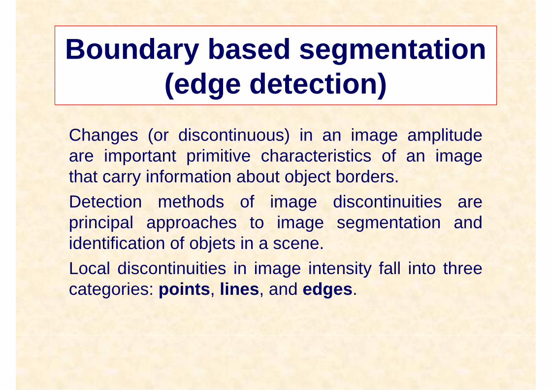
Boundary based segmentation (edge detection)
Changes (or discontinuous) in an image amplitude are important primitive characteristics of an image that carry information about object borders.
Detection methods of image discontinuities are principal approaches to image segmentation and identification of objets in a scene.
Local discontinuities in image intensity fall into three categories: points, lines, and edges.
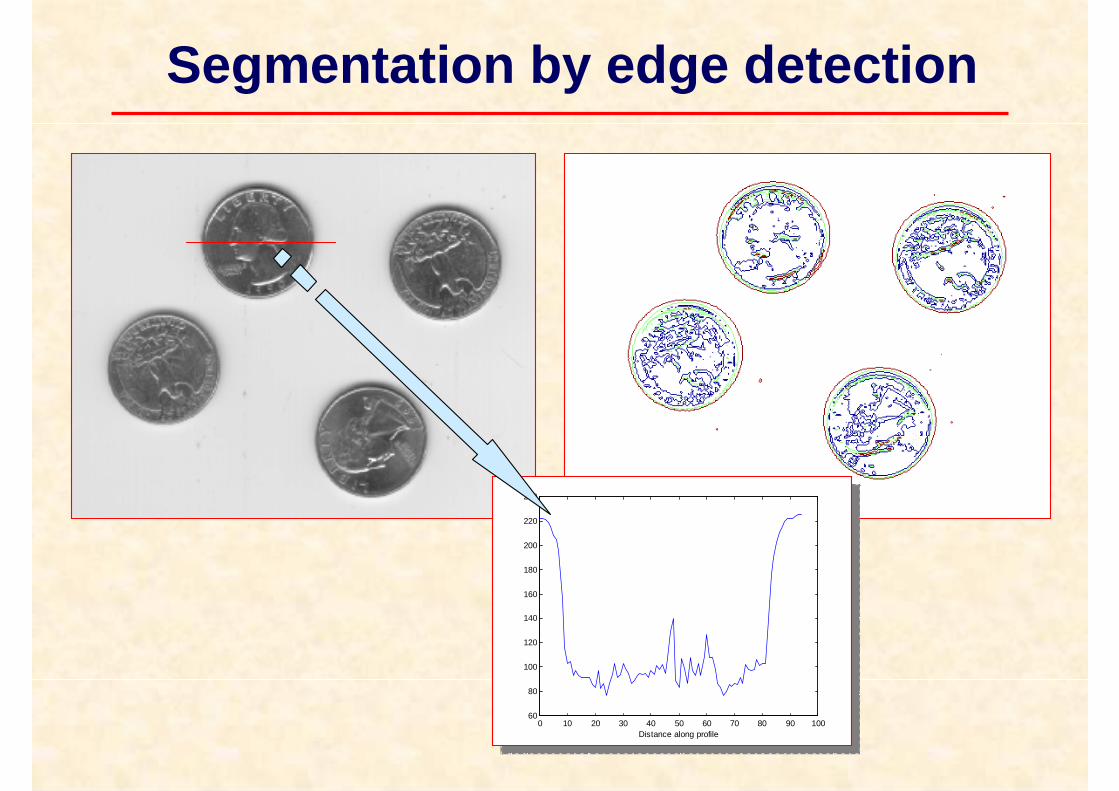
Segmentation by edge detection
0 10 20 30 40 50 60 70 80 90 10060
80
100
120
140
160
180
200
220
240
Distance along profile
0 10 20 30 40 50 60 70 80 90 10060
80
100
120
140
160
180
200
220
240
Distance along profile
Point and line detection
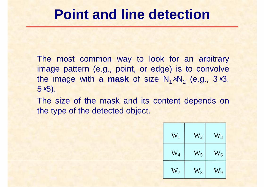
The most common way to look for an arbitrary image pattern (e.g., point, or edge) is to convolve the image with a mask of size N1×N2 (e.g., 3×3, 5×5).The size of the mask and its content depends on the type of the detected object.
W1
W4
W2
W5 W6
W3
W8 W9 W7
Detection masks
W1
W4
W2
W5 W6
W3
W8 W9 W7
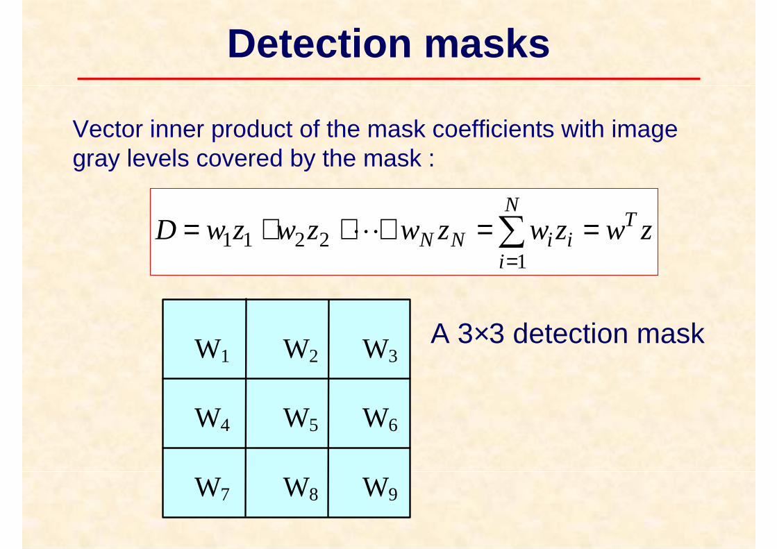
Vector inner product of the mask coefficients with image gray levels covered by the mask :
zwzwzwzwzwD TN
iiiNN ==+++= ∑
=12211 L
A 3×3 detection mask
-1
-1
-1
8 -1
-1
-1 -1-1
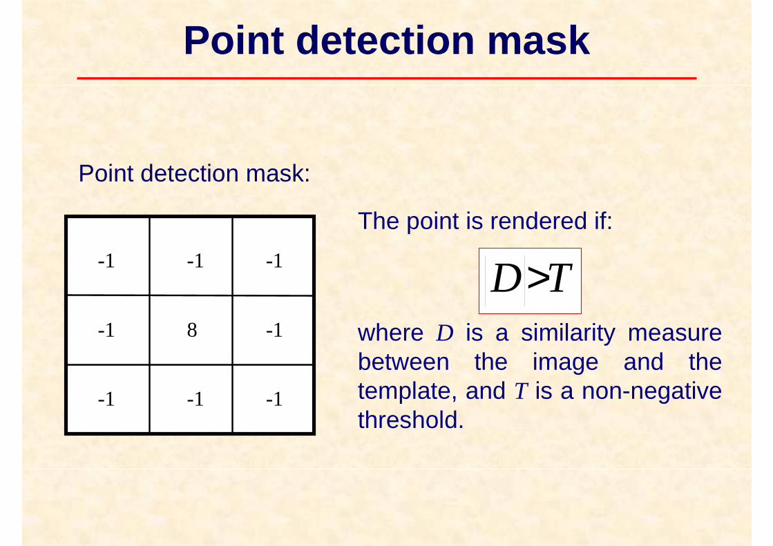
Point detection mask:
Point detection mask
The point is rendered if:
where D is a similarity measure between the image and the template, and T is a non-negative threshold.
TD>
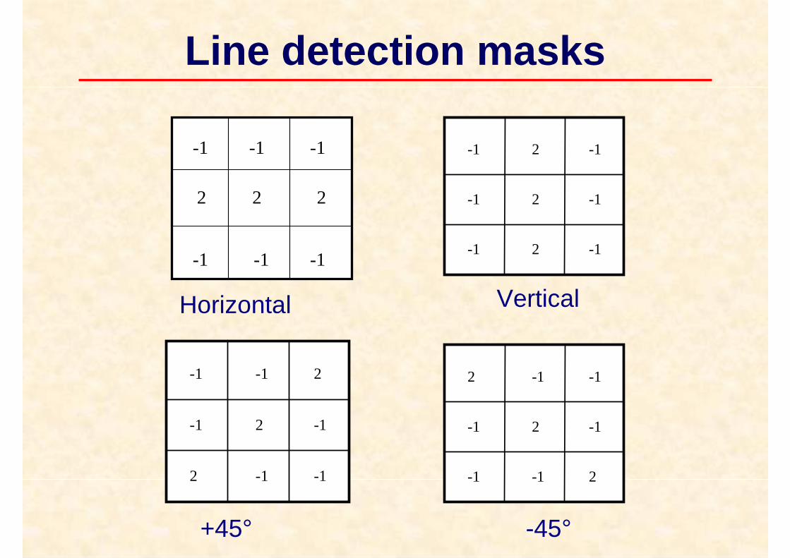
Line detection masks
-1
-1
2
2 -1
-1
2 -1-1
-1
-1
-1
2 -1
2
-1 -12
2
-1
-1
2 -1
-1
-1 2-1
Horizontal Vertical
+45° -45°
-1
2
-1
-1 -1
-1 -1
2 2
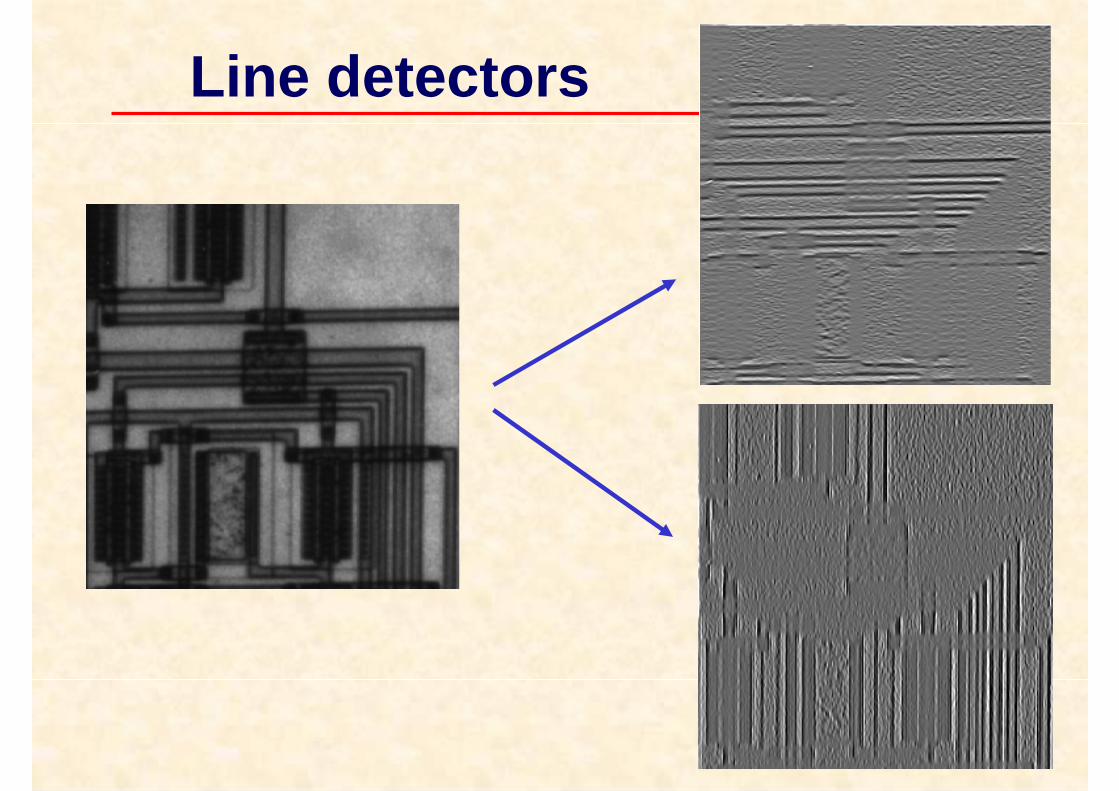
Line detectors
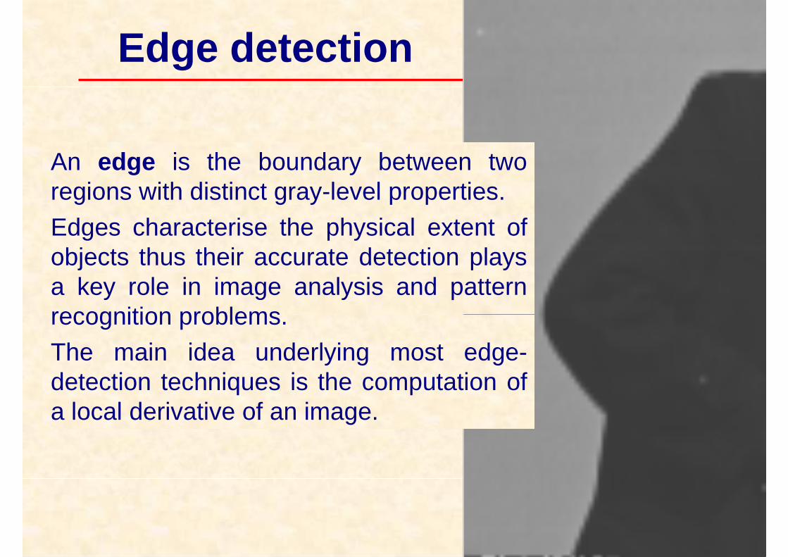
Edge detection
An edge is the boundary between two regions with distinct gray-level properties.
Edges characterise the physical extent of objects thus their accurate detection plays a key role in image analysis and pattern recognition problems.
The main idea underlying most edge-detection techniques is the computation of a local derivative of an image.
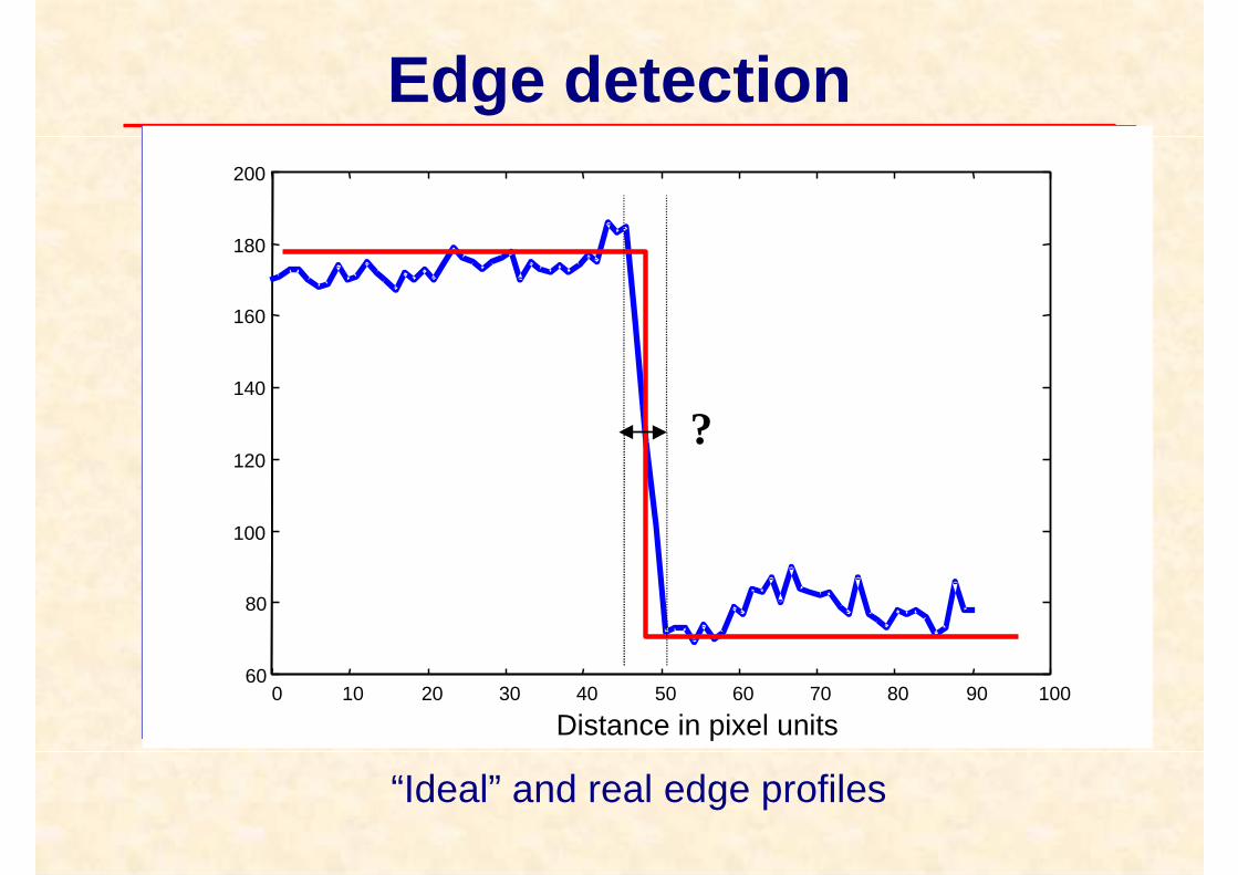
Edge detection
“Ideal” and real edge profiles
0 10 20 30 40 50 60 70 80 90 10060
80
100
120
140
160
180
200
Distance in pixel units
?
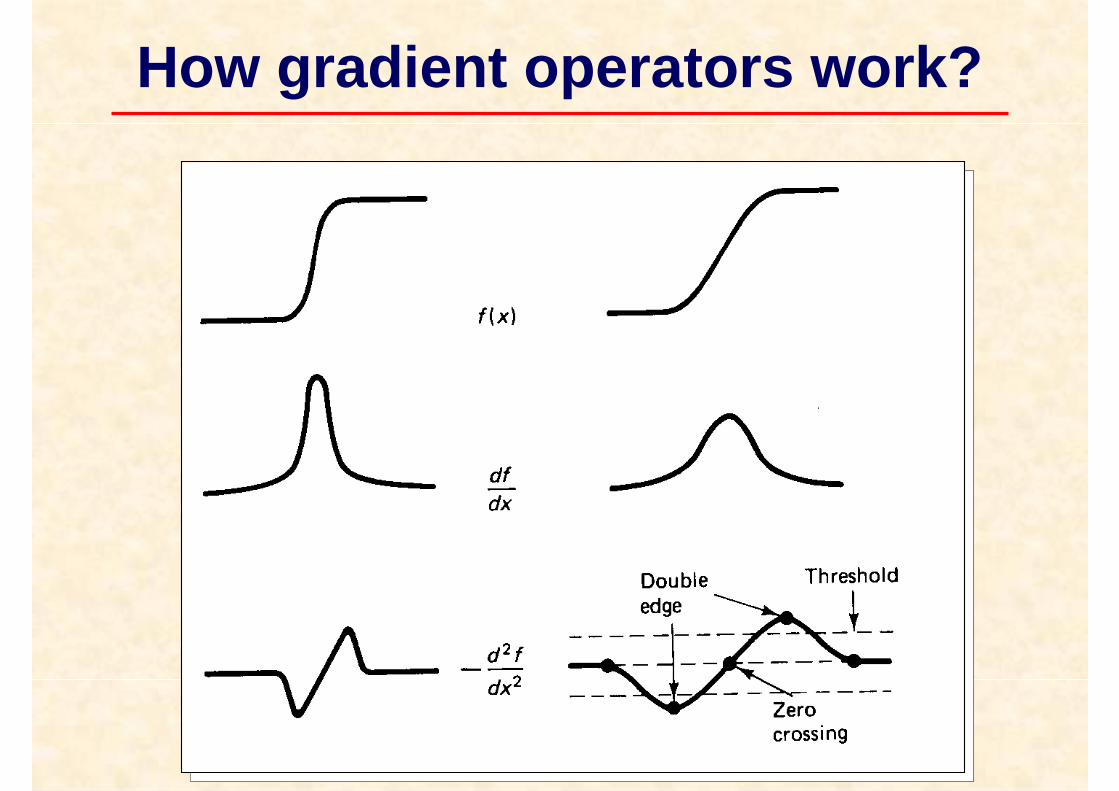
How gradient operators work?
v
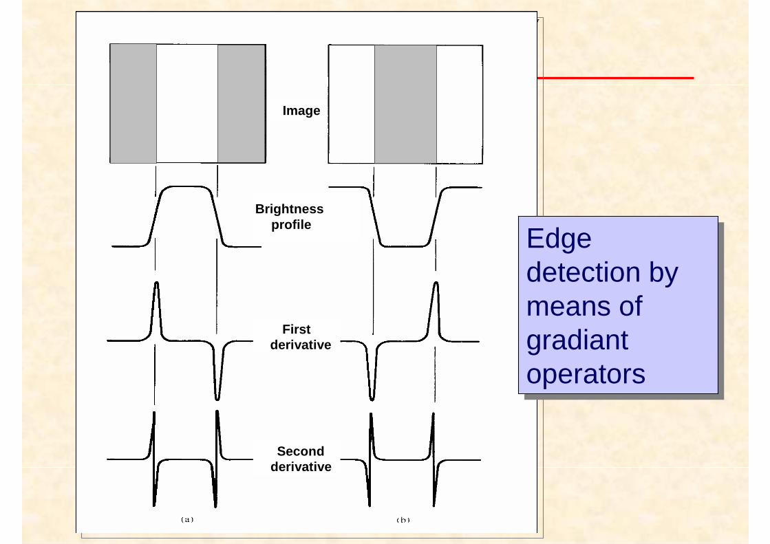
Image
Firstderivative
Secondderivative
Brightnessprofile
Edgedetection by means ofgradiantoperators
Edgedetection by means ofgradiantoperators
Edge detection
Note the following points about image derivative operators:
• the magnitude of the first derivative can be used to detect the presence of an edge in an image,
• the sign of the second derivative can be used to determine whether an edge pixel is on the dark or light side of an edge,
the second derivative has z zero crossing at the midpoint of a gray-level transition.
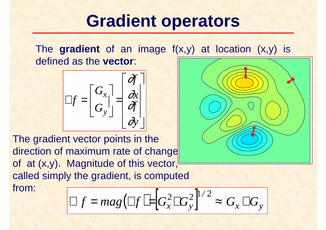
Gradient operators
=
=∇
y
fx
f
G
Gf
y
x
∂∂∂∂
The gradient of an image f(x,y) at location (x,y) is defined as the vector:
The gradient vector points in the direction of maximum rate of changeof at (x,y). Magnitude of this vector, called simply the gradient, is computedfrom:
( ) [ ] yx/
yx GGGGfmagf +≈+=∇=∇2122
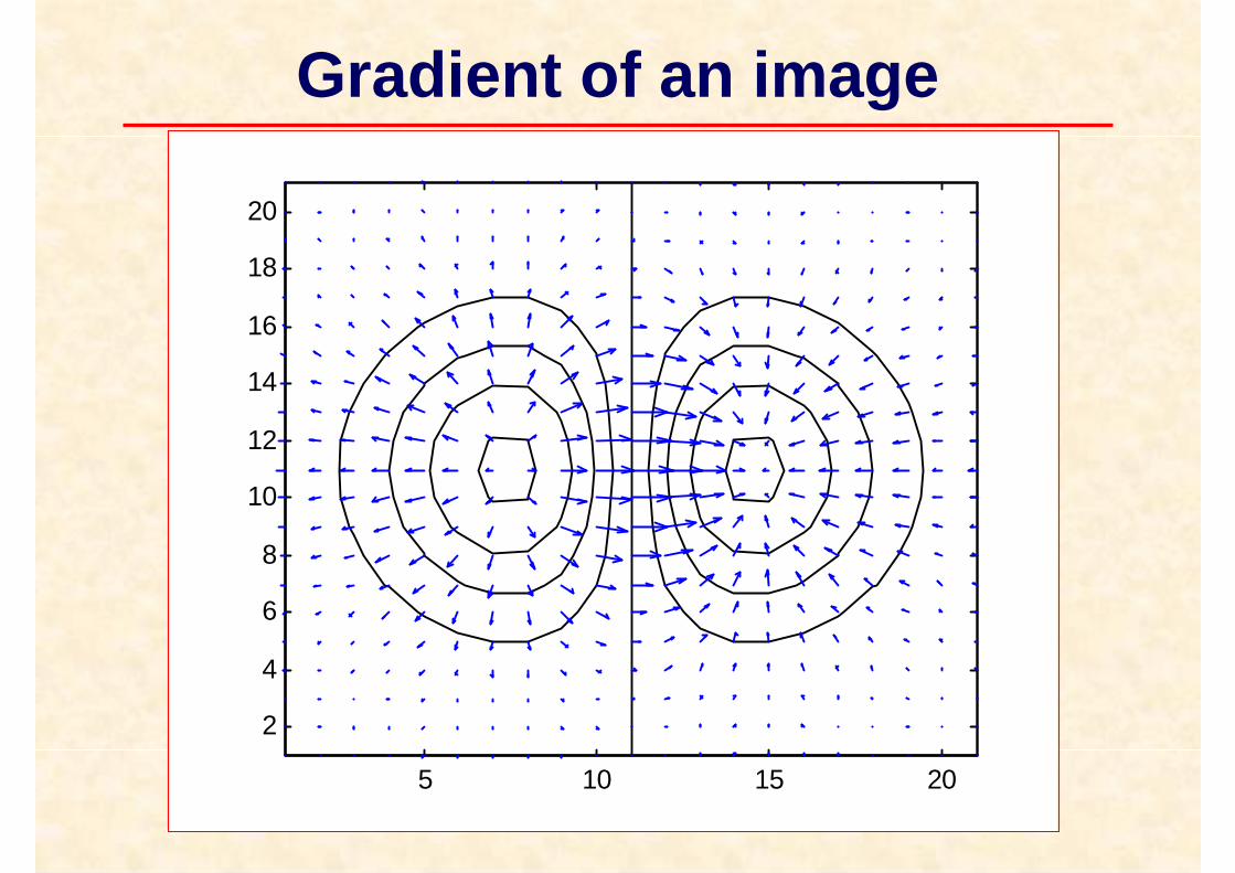
Gradient of an image
5 10 15 20
2
4
6
8
10
12
14
16
18
20
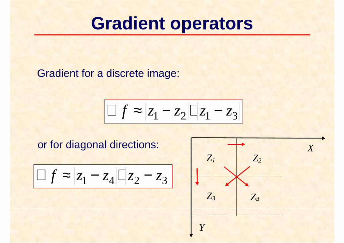
Gradient operators
Z1 Z2
Z3 Z4
X
Y
3121 zzzzf −+−≈∇
3241 zzzzf −+−≈∇
Gradient for a discrete image:
or for diagonal directions:
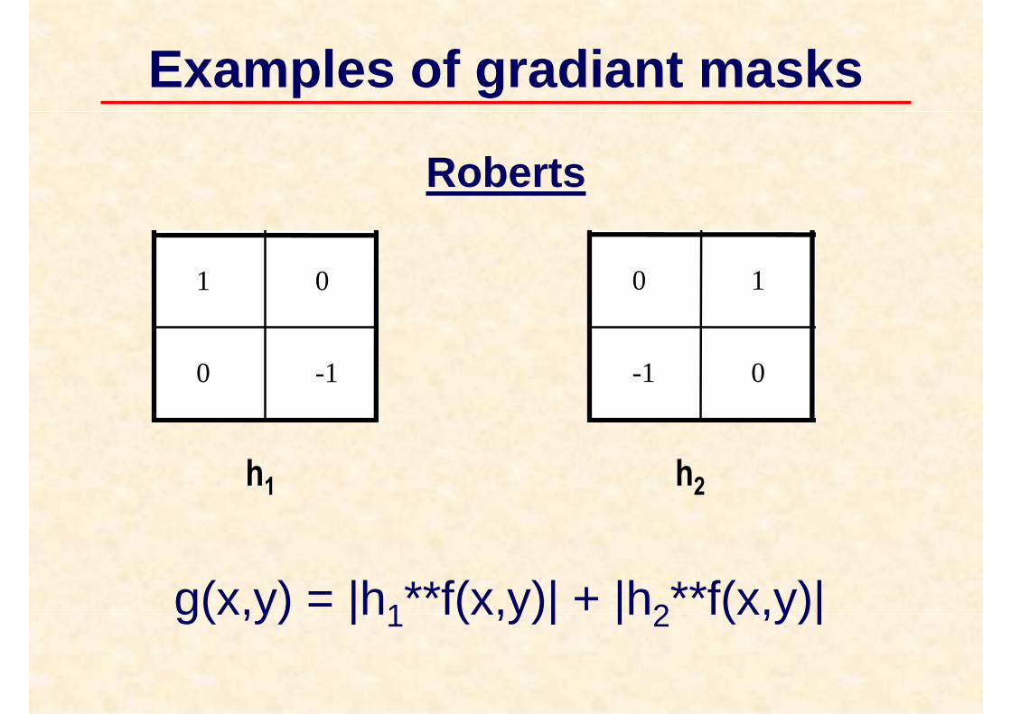
Examples of gradiant masks
Roberts
1 0
-10
h1
0 1
0-1
h2
g(x,y) = |h1**f(x,y)| + |h2**f(x,y)|
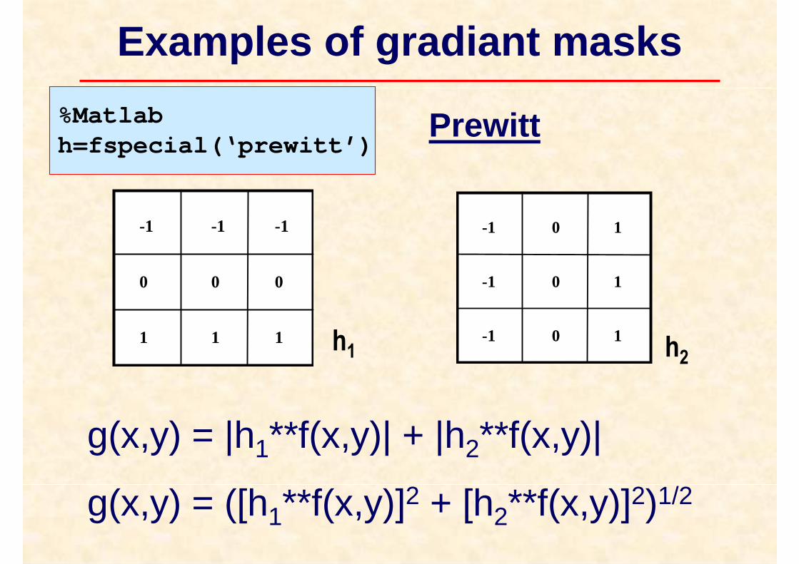
Examples of gradiant masks
-1
0
-1
0 0
-1
1 11
-1
-1
0
0 1
1
0 1-1
Prewitt
h1 h2
g(x,y) = |h1**f(x,y)| + |h2**f(x,y)|
g(x,y) = ([h1**f(x,y)]2 + [h2**f(x,y)]2)1/2
%Matlabh=fspecial(‘prewitt’)
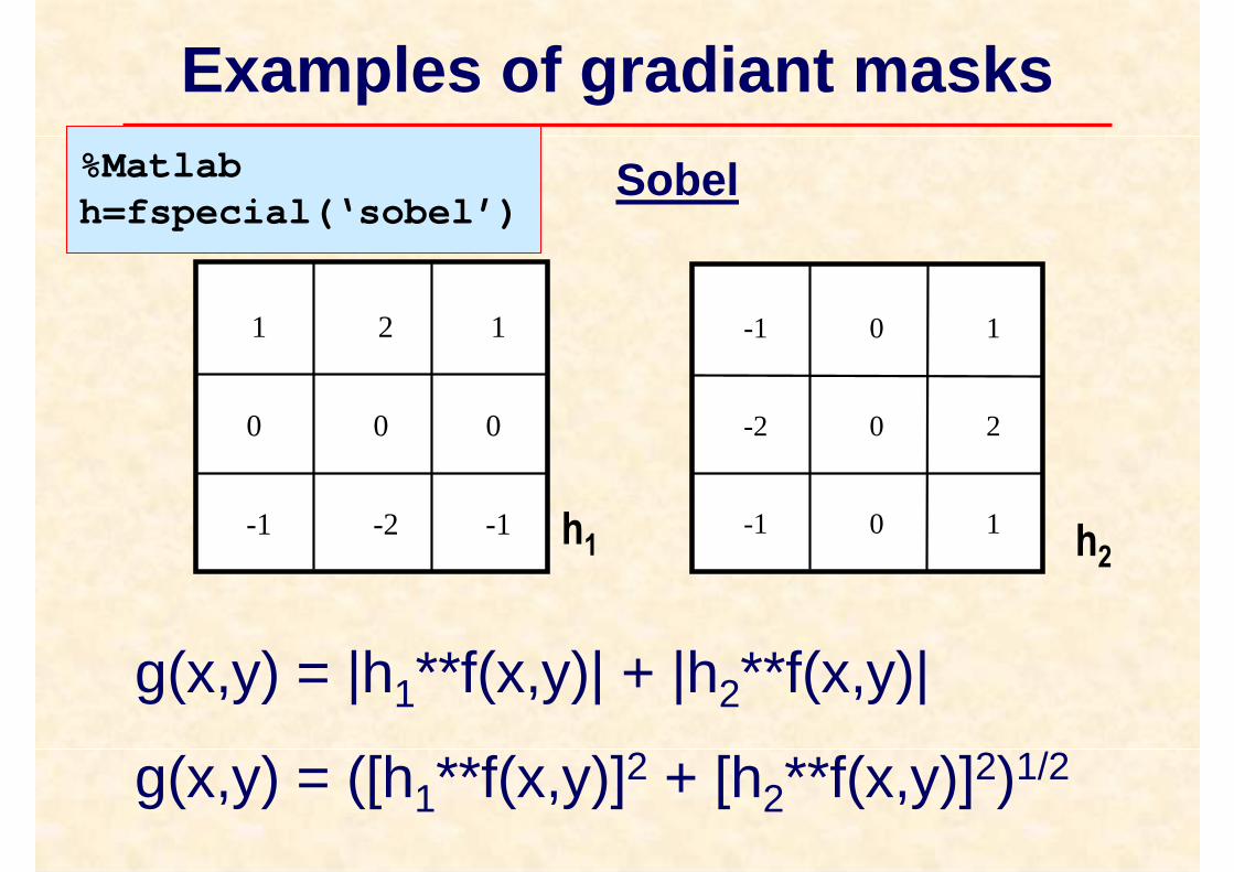
Examples of gradiant masks
Sobel
1
0
2
0 0
1
-2 -1-1 h1
-1
-2
0
0 2
1
0 1-1h2
g(x,y) = |h1**f(x,y)| + |h2**f(x,y)|
g(x,y) = ([h1**f(x,y)]2 + [h2**f(x,y)]2)1/2
%Matlabh=fspecial(‘sobel’)
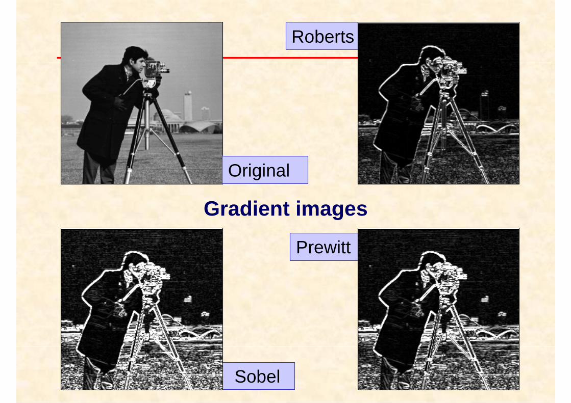
Sobel
Prewitt
Roberts
Original
Gradient images
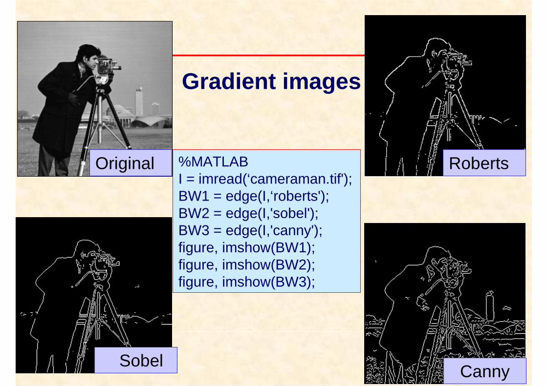
Original
Gradient images
Roberts
CannySobel
%MATLABI = imread(‘cameraman.tif');BW1 = edge(I,‘roberts');BW2 = edge(I,'sobel');BW3 = edge(I,'canny');figure, imshow(BW1); figure, imshow(BW2);figure, imshow(BW3);
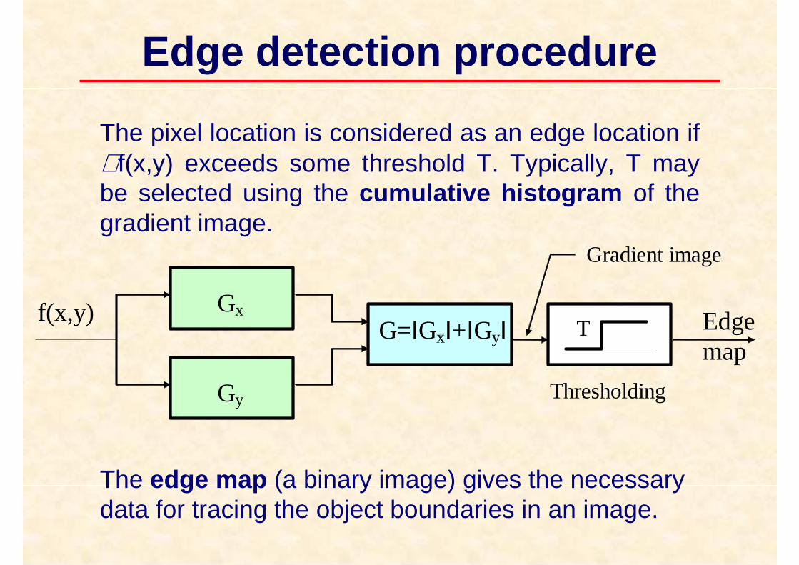
Edge detection procedure
The pixel location is considered as an edge location if ∇f(x,y) exceeds some threshold T. Typically, T may be selected using the cumulative histogram of the gradient image.
The edge map (a binary image) gives the necessary data for tracing the object boundaries in an image.
Gx
Gy
G=IGxI+IGyI f(x,y) Edge
map T
Thresholding
Gradient image
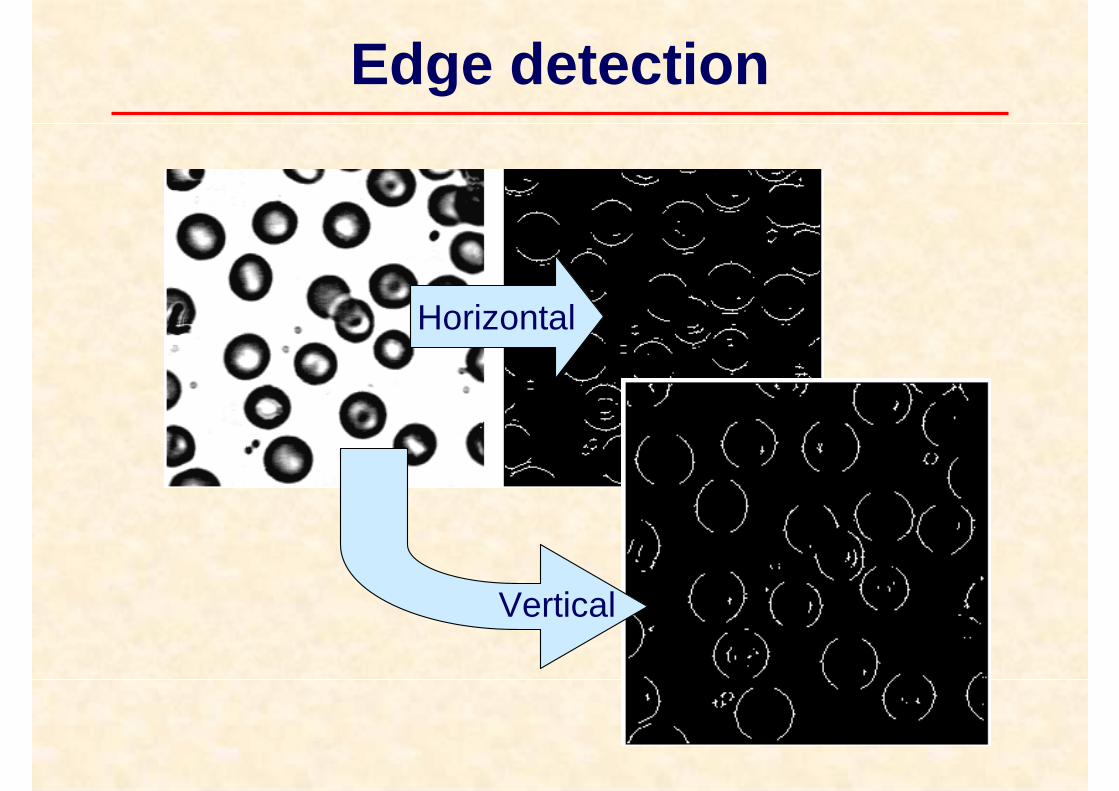
Edge detection
Horizontal
Vertical
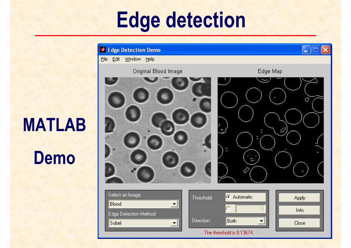
Edge detection
MATLAB
Demo
Laplacian
2
2
2
22
y
f
x
ff
∂∂
∂∂ +=∇
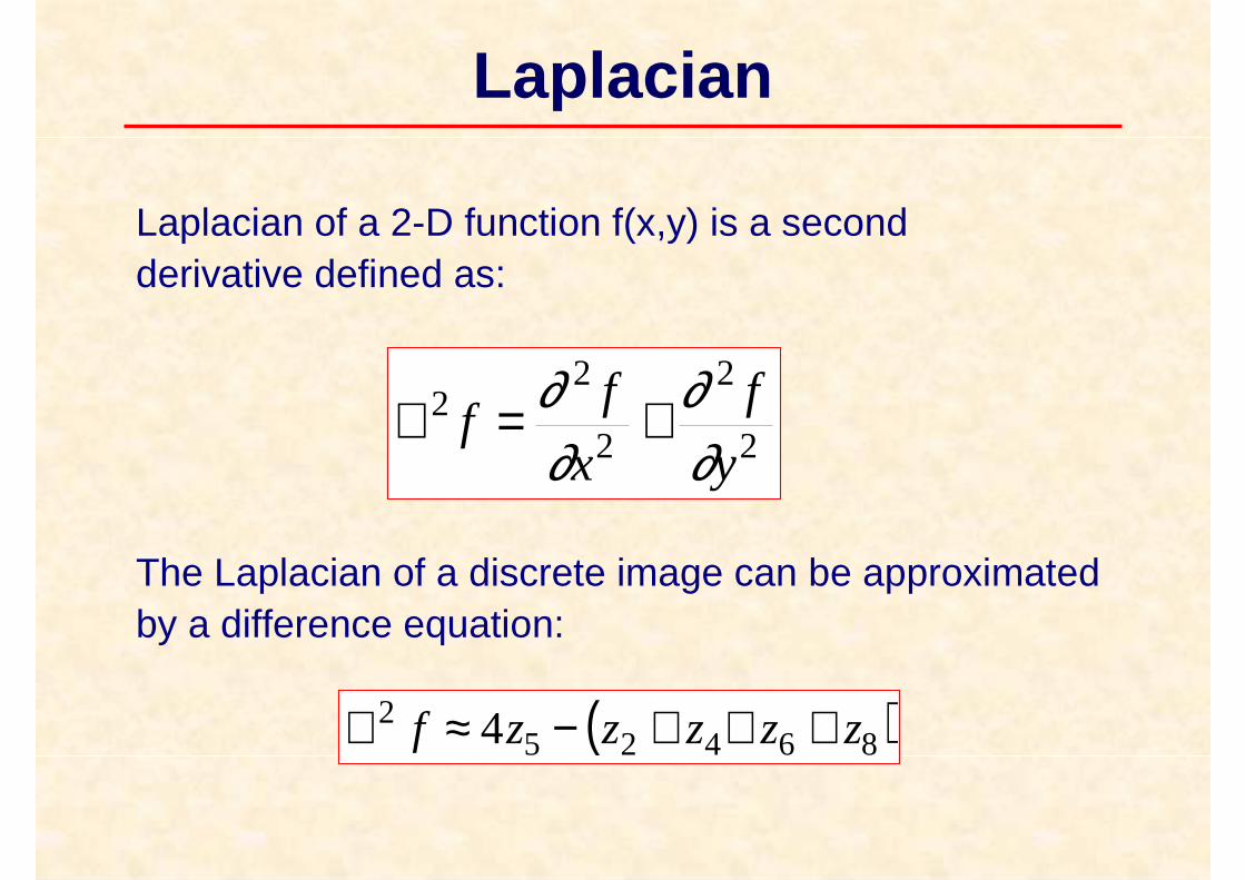
( )864252 4 zzzzzf +++−≈∇
Laplacian of a 2-D function f(x,y) is a second derivative defined as:
The Laplacian of a discrete image can be approximated by a difference equation:
Laplacian
-1
-1
-1
8 -1
-1
-1 -1-1
0
-1
-1
4 -1
0
-1 00
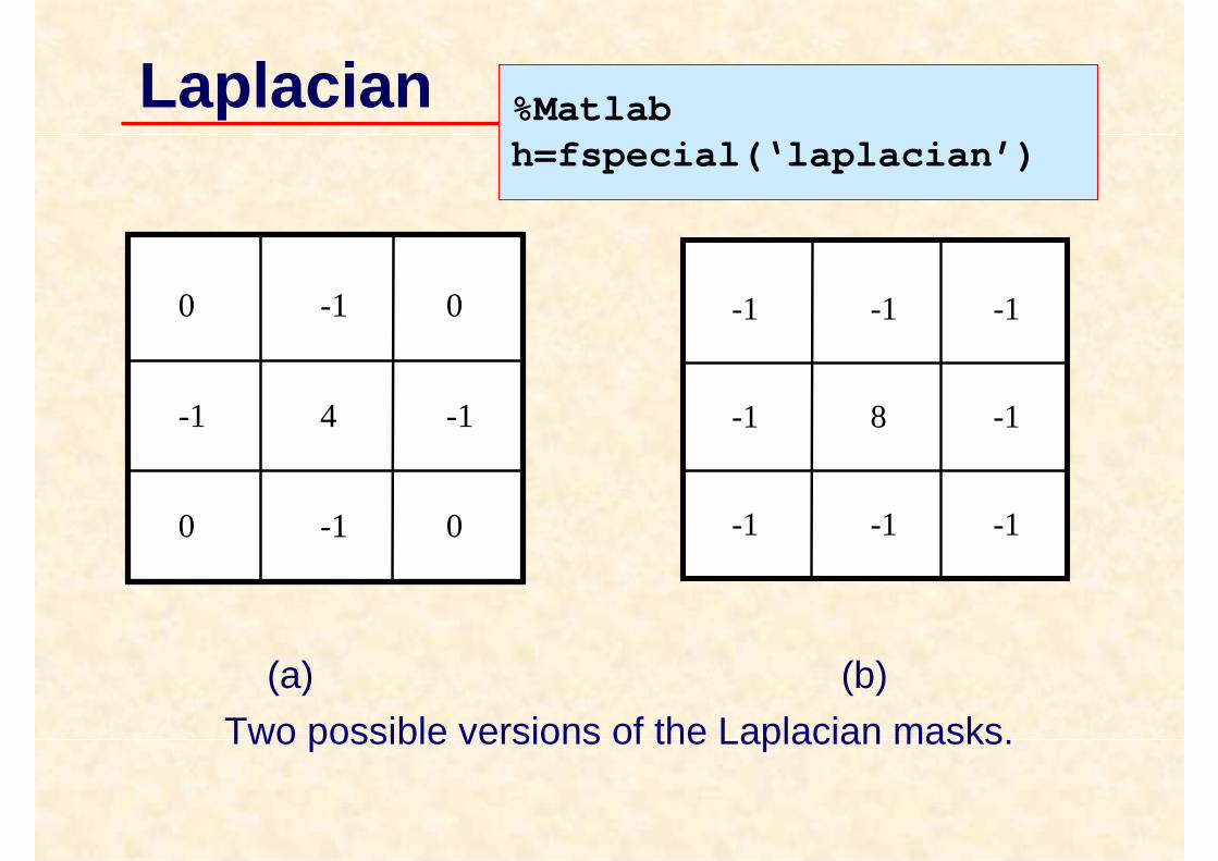
(a) (b)
Two possible versions of the Laplacian masks.
%Matlabh=fspecial(‘laplacian’)
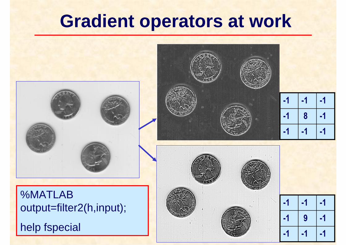
Gradient operators at work
-1-1-1
-18-1
-1-1-1
%MATLABoutput=filter2(h,input);
help fspecial-1-1-1
-19-1
-1-1-1
Laplacian in frequency domain
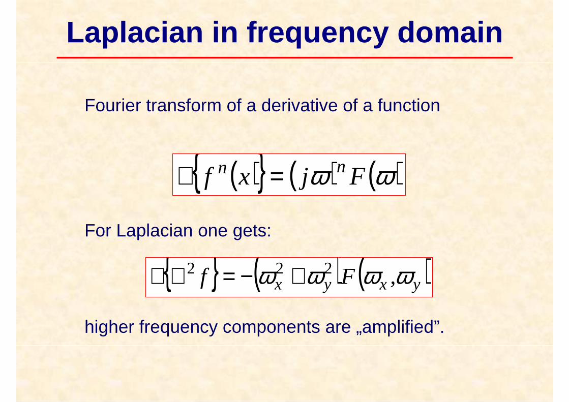
Fourier transform of a derivative of a function
( ){ } ( ) ( )ωω Fjxf nn =ℑ
For Laplacian one gets:
higher frequency components are „amplified”.
{ } ( ) ( )yxyx ,Ff ωωωω 222 +−=∇ℑ
Laplacian
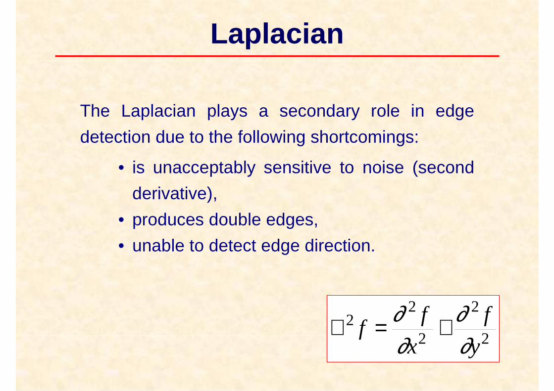
The Laplacian plays a secondary role in edge
detection due to the following shortcomings:
• is unacceptably sensitive to noise (second
derivative),
• produces double edges,
• unable to detect edge direction.
2
2
2
22
y
f
x
ff
∂∂
∂∂ +=∇
Laplacian
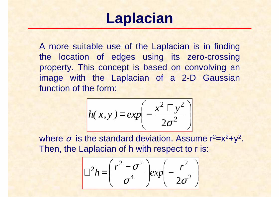
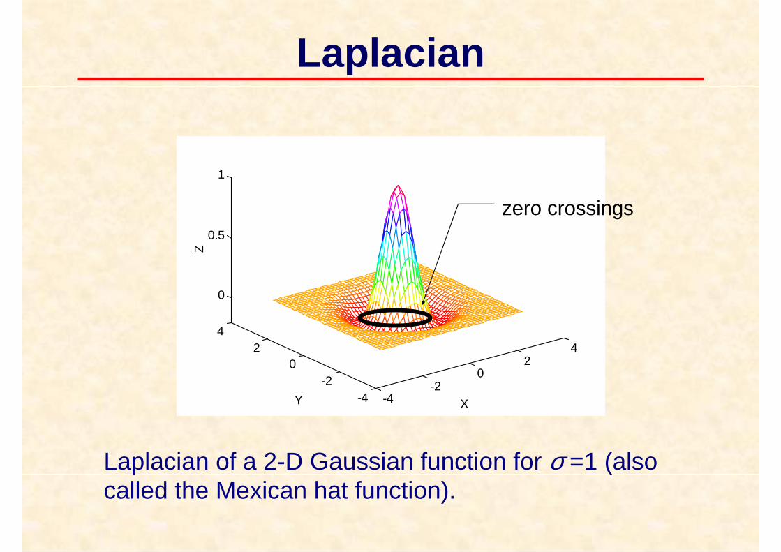
A more suitable use of the Laplacian is in finding the location of edges using its zero-crossingproperty. This concept is based on convolving an image with the Laplacian of a 2-D Gaussian function of the form:
+−= 2
22
2σyx
exp)y,x(h
where σ is the standard deviation. Assume r2=x2+y2. Then, the Laplacian of h with respect to r is:
−
−=∇ 2
2
4
222
2σσσ r
expr
h
-4-2
02
4
-4-2
02
4
0
0.5
1
XY
Z
Laplacian of a 2-D Gaussian function for σ =1 (also called the Mexican hat function).
Laplacian
zero crossings
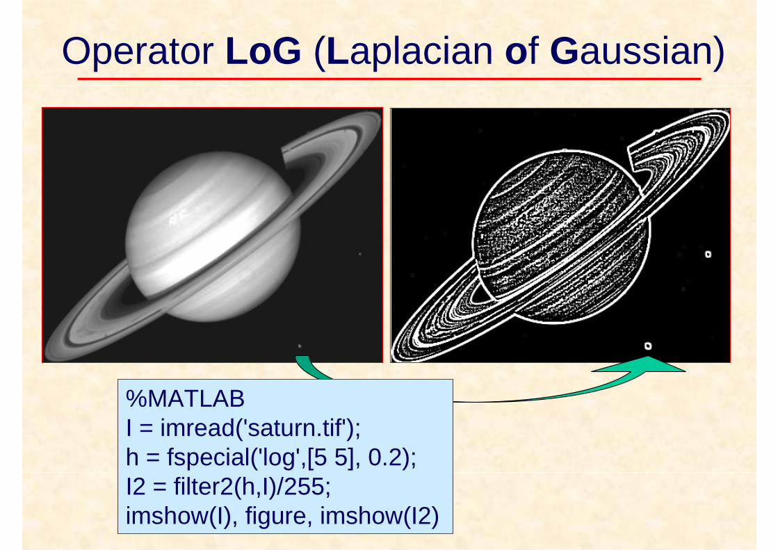
Operator LoG (Laplacian of Gaussian)
%MATLABI = imread('saturn.tif');h = fspecial('log',[5 5], 0.2);I2 = filter2(h,I)/255;imshow(I), figure, imshow(I2)
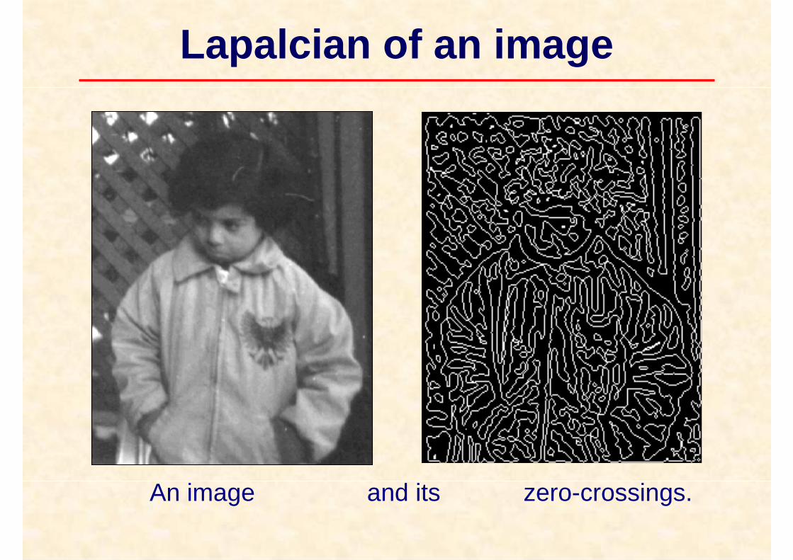
Lapalcian of an image
An image and its zero-crossings.