Loughborough UniversityInstitutional Repository

Boundary element methodsfor road vehicleaerodynamics

This item was submitted to Loughborough University's Institutional Repositoryby the/an author.

Additional Information:

• A Doctoral Thesis. Submitted in partial fulfilment of the requirementsfor the award of Doctor of Philosophy at Loughborough University.

Metadata Record: https://dspace.lboro.ac.uk/2134/26942

Publisher: c© N.A. Shah

Rights: This work is made available according to the conditions of the CreativeCommons Attribution-NonCommercial-NoDerivatives 2.5 Generic (CC BY-NC-ND 2.5) licence. Full details of this licence are available at: http://creativecommons.org/licenses/by-nc-nd/2.5/

Please cite the published version.

This item was submitted to Loughborough University as a PhD thesis by the author and is made available in the Institutional Repository

(https://dspace.lboro.ac.uk/) under the following Creative Commons Licence conditions.

For the full text of this licence, please go to: http://creativecommons.org/licenses/by-nc-nd/2.5/

LOUGHBOROUGH UNIVERSITY OF TECHNOLOGY

LIBRARY

AUTHOR/FILING TITLE

SH-A ~ N f\ . : -- ________ --------t -------------------- -------, I

--7 -- - ----- --.-------------- - - - -- --- - ---- - ------ --I ACCESSION/COPY NO. .

O/OIf-31/ 01 --------- - ------- ---- --- - --- -- - - - --- ---- -- - - -- - - --

VOL NO. CLASS MARK ,-LA'" CO Py

~

This book was bound by

Badminton Press 18 Half Croft, Syston, Leicester, LE7 8LD Telephone: Leicester (05331 602918.

"

,-

BOUNDARY ELEMENT METHODS FOR

ROAD VEHICLE AERODYNAMICS

by

NAWAZISH ALL SHAH

M.Sc. (PAK) , M.Sc. (U.K.)

A Doctoral Thesis

Submitted in partial fulfilment of the requirements

for the award of

DOCTOR OF PHILOSOPHY

of the Loughborough University of Technology

October, 1985

Supervisor: Dr. K.S. PEAT, B.Sc., Ph.D.

Department of Engineering Mathematics,

Loughborough ·University of Technology.

© by N.A. SIIAH (1985).

r---' -'~"""-5 L'n.:gt:iwr:;!J~h UniVafi~~Y'

of T 6cit:,,:(;1 :"'9)' Uhr!!':! i

Pm f' eAo. __ ' ~.~. __ l C!"~l . .,

Ace. I No. 0 I 0 i..pJ / 0 I

-2-

CERTIFICATE OF ORIGINALITY

This is to certify that I am responsible for the work submitted

in this thesis, that the original work is my own except. as

specified in acknowledgements or in footnotes, and that neither

the thesis nor the original work contained therein has been

submitted to this or any other institution for a higher degree.

-3-

DEDICATION

To my ~arents, wife and children

-4-

ACKNOWLEDGEHENTS

I begin in the name of Allah the most Beneficient, the most Herciful.

All praise be to Allah, who is the Lord of the whole universe and the

source of all knowledge. I thank Allah for giving me the strength and

energy to complete this work and making everything possible.

I am deeply indebted to Dr. K.S. Peat for his supervision,

guidance, help and encouragement at every stage during the progress of

my research work and in preparation of the manuscript of this thesis.

His invaluable suggestions and comments helped considerably in the

development of the work presented here. He has always been friendly

and cooperative and his readiness to assist me at all times has been

remarkable.

I would like to express my sincere thanks to all the staff of the

Engineering Hathematics Department for their help and cooperation,

in particular, to my Director of Research, Professor A. C. Bajpai, for

extending to me the departmental facilities and for his advice and help

on a number of occassions.

I wish to take this opportunity to express my gratitude to my

parents and mother-in-law for their patience, encouragement and

prayful blessings for my welfare and success. I am deeply grieved

for the death of my fath~r-in-law in my absence from Pakistan, who had

always wished 'for my higher education but can no longer witness this

thesis; my ultimate gratitude.

-5-

My deepest gratitude goes to my wife for her moral support,

constant encouragement and help throughout the course of my study.

Special thanks for my children who have made my stay in the U.K.

joyful.

I would like to thank BL Technology Ltd. for providing me with

the results of their wind tunnel tests over the models of car bodies.

Thanks are also due to the British Council for providing me the

financial support for the period of my studies in the U.K.

Finally, my thanks go to Mrs. Barbara Bell for her beautiful

typing of this thesis.

-6-

SU~:NARY

The technique of the "boundary element method consists of sub­

dividing the boundary of the field of a function into a series of

discrete elements, over which the function can vary. This technique

offers important advantages over domain type solutions such as finite

elements and finite differences. One of the most important

features of the method is the much smaller system of equations and the

considerable reduction in data required to run a program. Furthermore,

the method is well-suited to problems with an infinite domain.

Boundary element methods can be formulated using two different

approaches called the • direct' and the • indirect' methods.

In this thesis, the author has considered various formulations

of the boundary element method in the calculation of the potential flow

field around a road vehicle. In practice the potential flow sotution

must be followed by a boundary layer analysis, and repeated iteration

of both is required for a complete solution. Thus computational

efficiency of the boundary element method is of paramount importance

for this solution technique. The flowfield around a road vehicle is

semi-infinite, due to the presence of the ground plane, and is

characterized by a semi-infinite wake extending downstream of the

vehicle.

The results obtained using various boundary element methods have

been compared with analytical solutions for unbounded bodies,

bodies in the presence of a ground plane, and semi-infinite hodies, in

-7-

order to investigate their relative advantages in all relevant

situations. This has resulted in the development of a direct

boundary element method that can model the flow about several budies,

each of which may have a three-dimensional wake.

Finally, the 'direct' boundary element method has been applied

to calculate the flow around car body shapes and comparison between

computed results and experimental results which have been obtained

from models of car bodies is presented.

SECTION 1:

1.1

1.2

1.3

SECTION 2:

2.1

2.2

2.3

2.4

-8-

CONTENTS

Acknowledgements

Summary

Contents

List of'Symbols

INTRODUCTION

Statement of the problem

Literature Survey

Brief description of the method of

solution

CONSTITUTIVE EQUATIONS FOR THE BOUNDARY

ELEMENT METHODS

Introduction

Derivation of the equation for the

direct boundary element method

Formulation of the direct boundary

element method for an infinite

domain

Derivation of the equation for the

indirect boundary element method

4

6

8

12

15

19

29

32

33

39

42

SECTION 3:

3.1

3.2

3.3

3.4

3.5

SECTION 4:

4.1

4.2

4.2.1

4.2.2

4.2.3

4.3

4.4

4.4.1

4.5

SECTION 5:

5.1

5.2

5.3

-9-

DISCRETE ELEMENT FORMULATION OF THE

BOUNDARY INTEGRAL EQUATION

Introduction

Types of boundary elements

Matrix formulation

Evaluation of integrals

Solution of the system of equations

A DIRECT BOUNDARY ELEMENT METHOD

APPLIED TO POTENTIAL FLOW PROBLEMS

Introduction

Unbounded flow field calculations

Flow past a circular cylinder

Flow past a sphere

Flow past an ellipsoid of revolution

Effects of a ground plane

Modelling of a wake

Flow past a semi-infinite body

Comparison of Gauss-Elimination and

Gauss-Seidel methods

COMPARISON OF THE DIRECT AND INDIRECT

BOUNDARY ELEMENT METHODS

Introduction

Alternative forms of the indirect

boundary element method using

doublet distributions

Matrix formulation

46

47

56

64

69

71

72

72

89

93

101

105

113

117

137

139

141

5.4

5.4.1

5.4.2

5.4.3

5.5

5.6

5.6.1

5.7

5.8

SECTION 6:

6.1

6.2

6.3

6.4

SECTION 7:

7.1

7.2

-10-

Unbounded flow field calculations

Flow past a circular cylinder

Flow past a sphere

Flow past an ellipsoid of revolution

Effects of a ground plane

Modelling of a wake

Flow past a semi-infinite body

Comparison of computing times

Conclusions

COMPARISON OF "INTEGRATION SCHEMES FOR

VARIOUS TYPES OF ELEMENTS

Introduction

Modified quadrature formulae for elements

with singu1arities

Comparison of Gauss-"quadrature and

modified quadrature schemes

Comparison of types of elements

APPLICATION TO ROAD VEHICLES

Introduction

Comparison of experimental and computed

pressure coefficients over the surface. of

a model car body with

142

143

152

153

154

155

160

162

163

166

167

194

196

207

207

SECTION 8:

(i)

(ii)

(iii)

-11-

Vertical back

Short Taper

Long Taper

CONCLUSIONS AND SUGGESTIONS FOR

FURTHER WORK

References

209

210

211

235

238

-12-

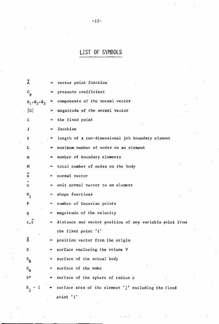
LIST OF SYMBOLS

... A = vector point function

c = pressure coefficient p

gl,g2,g3 = components of the normal vector

lel = magnitude of the normal vector

i = the fixed point

J = Jacobian

R, = length of a two-dimensional j th boundary element

L

m

M

-+ n

n

N. 1

p

maximum number of n.odes on an element

= number of boundary elements

= total number of nodes on the body

= normal vector

= unit normal vector to an element

= shape functions

number of Gaussian points

q = magnitude of the velocity

... r,r = distance and vector position of any variable point from

the fixed point 'i'

... R = position vector from the origin

S surface enclosing the volume V

SB = surface of the actual body

Sw surface of the wake

S* surface of the sphere of radius p

S. - i J

surface area of the element 'j' excluding the fixed

point 'if

... t

t

u

v

w p

x, y

(xq,yq)

(x. ,y.) 1 1

X,Y,Z

<p'

<p. 1

·<p c •c

<Psphere

<p o . e

<P s • inf

-13-

= tangent vector

unit tangent vector

speed of the uniform stream

volume of the region R. Also used as the velocity

Gaussian weighting coefficients

= starting point of the wake

= cartesian plane coordinates

coordinates of the variable point 'Q'

= coordinates of the fixed point 'i'. Also used as the

nodal values of the variables x and y

coordinates of the extreme points of the boundary

elements

= coordinates of the mid-point of the two-dimensional

boundary elements

= cartesian, space c60rdinates

= velocity potential in the region R. Al so used as a

scalar point function

velocity potential in the region R'

= value of the velocity potential <P at the fixed point

Also used to denote the nodal values of the variable

, . , 1 •

cp

= perturbation velocity potential of the circular cylinder

perturbation velocity potential of the sphere

= perturbation velocity potential of an ovary ellipsoid

= perturbation velocity potential of the semi -infinite body

= velocity potential of the uniform stream

= value of the velocity potential at infinity

= total velocity potential of the flow

-14-

r boundary of a two-dimensional region

r. J

surface of the jth element

p = radius of the sphere

o = source strength

= doublet strength

= stream function. Also used as a scaler point function.

e = angle between the radius vector and the x-axis

r,e polar coordinates in two-dimensions

= local coordinate system on an element

coordinates of the kth node on the element

= coordinates of the pth Guassian point

p,9,n = spherical polar coordinates in section (2.3)

x,w,w = cylinderical polar coordinates in section (4.4.3)

-15-

SECTION 1

INTRODUCTION

1.1 STATE~lliNT OF THE PROBLEM

The problem considered in this thesis is to calculate the flow

field around a road vehicle using the boundary element method.

Basically the aim is to calculate the velocity and the pressure

distribution on the surface of the vehicle which result from its motion

through the atmosphere. It will be assumed that the speed at which

the vehicle is moving is constant. In fluid mechanics, the problem

of the uniform rectilinear motion of a body through a fluid at rest

at infinity and that of the onset flow uniform at infinity disturbed by

the introduction of the same body he Id at rest are dynamically

equivalent. The force experienced by the body in the first case is

equal in magnitude and opposite in direction to the force required to

hold the body at rest in the second case. For convenience, the vehicle

body is regarded as being stationary and immersed in an infinite volume

of the uniform onset flow. The uniform onset flow is defined as the

one which would exist in the absence of the body and is taken as a

uniform stream of unit magnitude. The component of the resultant

force exerted by the fluid on the body in the direction of the uniform

. onset flow of the fluid is called the drag force, ",hilst the component

of the resultant force in the direction normal to the flow direction is

-16-

called the lift force.

The flow around road vehicles is of low Mach number, therefore it

can be considered as incompressible. Furthermore, this flow is of

high Reynolds number which implies that the viscosity of the fluid has

neglibible effect except very near to the body surface, where a thin

boundary layer will exist. Thus, provided that there is no input

vorticity in the free stream, the whole of the flow field exterior to

the thin boundary layer can be considered to be irrotationa1. The

assumptions of incompressible and inviscid flow cause great

simplifications to the general equations of aerodynamics. The

resultant potential flow analysis will give a first approximation to

the real flow field, and this approximation can later be refined

through the use of boundary layer solutions.Since the flow can be

considered incompressible, the equation of continuity becomes-

div V = 0 (1. 1)

+ where V is the velocity of the fluid at any point of the flowfield.

Further, if the flow is taken to be irrotational, then

4-V = -grad <I> (1. 2)

where <I> is the total velocity potential of the flowfield.

From equations (1.1) and (1.2), it follows that

(1. 3)

which is Laplaces equation,

The boundary condition on the surface S of the body 1S derived from the

requirement that on a stationary impervious surface S, the normal

component of the fluid velocity is zero. Thus,

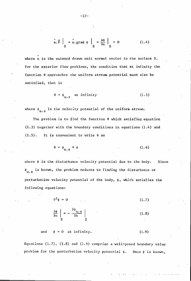
-17-

• + n.V

s s = an = 0 (1. 4) = n.grad 1>

s

where n is the outward drawn unit normal vector to the surface S.

For the exterior flow problems, the condition that at infinity the

function 1> approaches the uniform stream potential must also be

satisfied, that is

1> -> </> at infini ty u.s

(1. 5)

where </> is the velocity potential of the uniform stream. u. s .

The problem is to find the function 1> which satisfies equation

(1. 3) together with the boundary conditions in equations (1.4) and

(1.5). It is convenient to write ~ as

(1. 6)

where </> is the disturbance velocity potential due to the body. Since

</> is known, the problem reduces to finding the disturbance or u. s

perturbation velocity potential of the body, </>, which satisfies the

following equations:

(1. 7)

~'I = -an (1. 8)

S S

and </> + 0 at infinity. (1. 9)

Equations (1.7). (1.8) and (1.9) comprise a well-posed boundary value

problem for the perturbation velocity potential </>. Once $ is known,

-18-

the total velocity potential 4> of the flow can be found from equation

-> (1. 6) and the velocity V of the flow field is given by equation (1.2).

The pressure coefficient C at any point on the surface of the body p

can then be found from Bernoulli's equation which reduces to

C = 1 - ( V )2 = 1 _ V2 P U

(1.10)

since the speed U of the uniform stream has been taken as unity.

For a body such as a road vehicle, which lies near the ground,

simulation of the ground flow is an important feature to be

incorporated into the theory. The inviscid flow over the ground,

which is considered to be a plane, remains everywhere tangential to its

surface. This flow is simulated by the so called "mirror image"

principle. A mirror image of the vehicle is imagined to be present

below the ground. The flow around the vehicle and its image is then

symmetrical with respect to· the ground plane. The plane of synmetry

is a streamline or stream surface and represents the inviscid flow

over the ground.

The real flow field around a road vehicle is further characterized

by the presence of a wake which starts from the rear end of the body

and extends to infinity in the direction of the onset flow. This

wake is due to the separation of the boundary layer from the surface

of the body and the boundary layer is caused by the viscosity of the

fluid. If the fluid were truly ideal then there would be no

boundary layer and no wake and hence there would be no drag on an obj ect

immersed into the flowing fluid. Whilst the wake is caused by

separation of the boundary layer, it is of much larger ·scale and

hence larger influence on the total flow field than is the boundary

-19-

layer. Thus even a first attempt at a potential flow solution must . . . include some app~1mat1on to account for the existence of a wake.

The technique used in this thesis is to model the separation stream

surface containing the wake as a continuation of the true body surface,

which will then extend to infinity.

1.2 LITERATURE SURVEY

The role of vehicle aerodynamic is of growing importance for the

design of vehicles, see for example Hucho [1) and Landahl [2). At

present, the study of vehicle aerodynamic is based almost sulely on

empirical methods, the wind tunnel being the most essential design

tool. Almost all major automanufacturers operate their own wind

tunnels, most of which are suitable for full-sized cars. The

current capital cost of a wind tunnel for full-sized cars is around

ten million pounds and the running costs of a tunnel are of the order

of thousands of pounds per hour. Thus there is great potential cost

benefit in the development of any system which can eliminate or

reduce the need for wind tunnel tests. In recent years, a few

attempts have been made to calculate the flow field around road

vehicles with the aid of theoretical methods. The work presented 1n

this thesis is a step in this direction. The author is well aware ef

the fact that a more sophisticated flow model than the one outlined

here is needed, if it should be applicable as a design tool. It seems

doubtful that the theoretical methods will completely replace the wind

tunnel tests on road vehicles in the foreseeable future. However,

theoretical methods can feasibly be developed to a stage where they

-20-

can be used as a guide to the basic aerodynamic design of road

vehicles, thus reducing the amount of wind tunnel testing required

and the cost of major design changes at a late stage of development.

It therefore appears that the theoretical methods will be of

increasing importance in the calculation of the flow field around

road vehicles. At present the available theoretical methods for the

flow field calculations are the methods of finite difference (Hirt and

Ramshaw [3], Markatos [4] and Demuren and Rodi [5]), finite elements

Ecer [6] and boundary elements.

Boundary element methods offer important advantages over the

'domain' type methods such as finite elements or finite differences.

One of the advantages is that with boundary elements one only has to

define the surface of the body, whereas with field methods it 1S

necessary to mesh the entire flow field. The amount of input data

for a boundary element method is therefore significantly less than for

a field method, which is a very important advantage in practice, as

mani hours can be spent in preparing and checking the data for finite

element or finite difference programs. Furthermore, for a g~ven

problem the boundary element method will have a much smaller system

size than a field method, and will therefore be computationally more

efficient. Boundary element methods are also well-suited to solve

problems where some boundary conditions are applied at infinity, as is

the case for exterior vehicle aerodynamics. In this thesis

attention will be given only to boundary element methods.

Over the past few years the importance of boundary elements have

been widely recognised and numerous papers and other works have been

published in this field. These methods are presented under different

names such as 'panel methods', 1 surface singularity methods',

-21-

'boundary integral equation methods' or 'boundary integral solutions'.

The name 'boundary element methods', which has originated from

Southampton University, describes the basic technique of the method

which consists in subdividing the boundary of the region under

consideration into a series of elements. These methods have been

successfully applied in a number of fields, for example elasticity,

potential theory, elastostatics and elas'todynamics, see Brebbia [26].

Boundary element methods can be formulated using two different

approaches called the 'direct' method and the 'indirect' method.

For potential flow problems, the direct method can be expressed in the

form of an integral equation which relates the value of the 'potential

at any point within the flow field with the values of the potential

and potential derivatives over the surface of the body and thus the

unknowns are calculated in the form of potential and potential

derivatives over the body surface. On the other hand, the indirect

method is based on the distribution of singularities, such as sources

or doublets, over the surface of the body and computes the unknowns

in the form of singularity strengths.

The indirect method has been used for many years in the past for

flow fiel.d calculations due to its simplicity. The first work on

flow field calculations around three-dimensional bodies is probably

that by lIess and Smith [7] and [8]. Their method, utilized a constant

source distribution over the surface of the body and is therefore

classified as a 'lower-order indirect' method. Host of the work on

flowfield calculations using boundary element methods has been done in

the field of aircraft aerodynamics. Over the past decade,' boundary

element methods have seen a trend towards higher-order formulations,

for which the singularity strength and / or geometry can vary over an

-22-

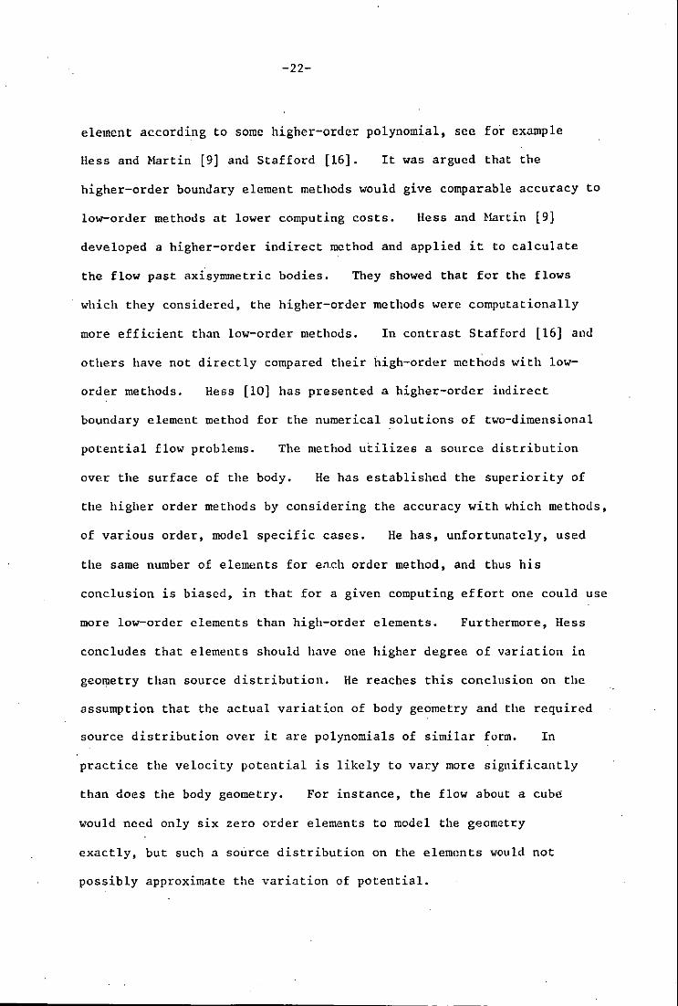
element according to some higher-order polynomial, see for example

lIess and Martin [9] and Stafford [16]. It was argued that the

higher-order boundary element methods would give comparable accuracy to

low-order methods at lower computing costs. lIess and ~illrtin [9]

developed a higher-order indirect method and applied it to calculate

the flow past axisymmetric bodies. They showed that for the flows

which they considered, the higher-order methods were computationally

more efficient than low-order methods. In contrast Stafford [16] and

others have not directly compared their high-order methods with low­

order methods. Hess [10] has presented a higher-order indirect

boundary element method for the numerical solutions of two-dimensional

potential flow problems. The method utilizes a source distribution

over the surface of the body. He has established the superiority of

the higher order methods by considering the accuracy with which methods,

of various order, model specific cases. He has, unfortunately, used

the same number of elements for en-ch order method, and thus his

conclusion is biased, in that for a given computing effort one could use

more low-order elements than high-order elements. Furthermore, Hess

concludes that elements should have one higher degree of variation in

geometry than source distribution. He reaches this conclusion on the

assumption that the actual variation of body geometry and the required

source distribution over it are polynomials of similar form. In

practice the velocity potential is likely to vary more significantly

than does the body geometry. For instance, the flow about a cube

would need only six zero order elements to model the geometry

exactly, but such a source distribution on the elements would not

possibly approximate the variation of potential.

-23-

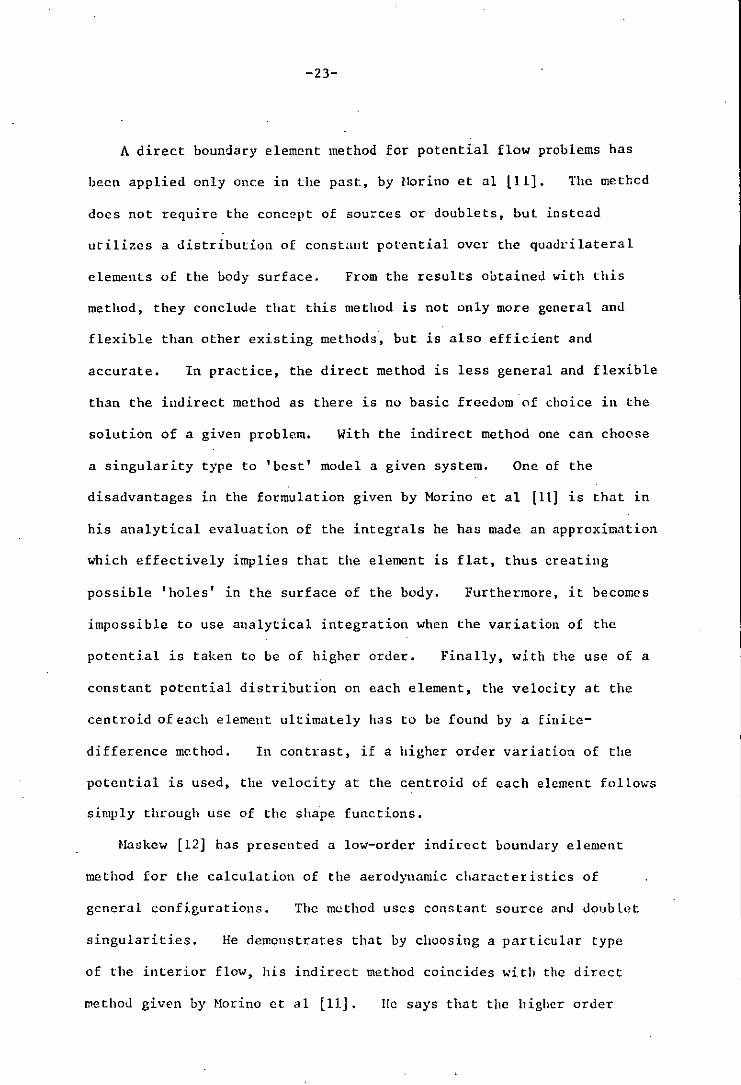
A direct boundary element method for potential flow problems has

been applied only Once in the past, by llorino et al [11]. The methcd

does not require the conc:?pt of sou;:.-ces or doublets, but instead

utilizes a distribution of constaut potential over the qua.drilateral

elements of the body surface. From the results obtained with this

method, they conclude that this method is not only more general and

flexible than other existing methods·, but is also efficient and

accurate. In practice, the direct method is less general and flexible

than the indirect method as there is no basic freedom·of choice in the

solution of a given problem. With the indirect method one can choose

a singularity type to 'best' model a given system. One of the

disadvantages in the formulation given by Morino et al [11] is that in

his analytical evaluation of the integrals he has made an approxillkqtion

which effectively implies that the element is flat, thus creating

possible 'holes' in the surface of the body. Furthermore, it becomes

impossible to use analytical integration when the variation of the

potential is taken to be of higher order. Fina 11y, wi th the use of a

constant potential distribution on each element, the velocity at the

centroid of each element ultimately has to be found bya finite-

difference method. In contrast, if a higher oruer variation of the

potential is used, the velocity at the centroid of each element follows

simply through use of the shape functions.

Maskew [12] has presented a low-order indirect boundary element

method for the calculation of the aerodynamic characteristics of

general configurations. Tbe m"thod uses constant source and doublet

singularities. He demonstrates that by choosing a particular type

of the interior flow, his indirect method coincides with the direct

method given by Horino ct al [ll]. lie says that the higher order

-24-

methods are not advantageous in reGions of close interaction between

singularities, where the main factor affecting the. solution accuracy

is the density of cc-ntrul points (points where the zero normal veloc.ity

. boundary conditiun is satisfied), while the order of the singularity

distribution has only a small in (l'"cnce . Maskew has formed the

judgement on the comparison of high order versus low-order

formulations for the numerical solution of a two-dimensional problem

·of a vortex positioned close to a right-angled corner. From tIle

comparisuns of his computed results with an analytical solution, he

concludes that the low-order boundary element method gives comparable

accuracy at 10\,or computing C03ts than higher-order methods. It

should be noted that t.he choice of a non-curved boundary for this test

case favours the low-order methods, in the sense that one of the maLn

theoretical aJvantag~s of a high-urder method is its ability to closely

model curved boundaries.

In addition to the main applicati.on of boundary element methods in

the calculation of the flow field around aircraft, they have also been

applied to cnlculate the flow field around trains and road vehicles.

The first werk on calculating the flow field around road vehicles was

by Stafford [13]. 1Ii) used the indirect boundary element method with

a di.stribution of vortex circuits over the surface of the body and

,over a postulated wake. The ml3thod predicts nclequately tbc pr~ssu)~C

distribution only ill the attached flow region. Ahmed and Hucho [14]

and Berta et al [15] hnve also used the 10l,-order indirect boundary

element methods for the calculation of flow field around road vehicles.

Ln the former case the length of the wake waS taken to be equal to the

length of the vehiCle and both of these were diseretized into flat

quadrilateral elements. The body surface was covered with a

-25-

distribution of sources and the wake surface was covered with

doublets. It was found necessary to extend the wake inside the body

surface in order to remove numerical problems at the body/wake

interaction region. The method then gave fairly good predictions of

the pressure distribution over that part of the body where the flow

remained attached. The drawback of this method is that the wake

model contributes as much to the overall system size as does the body

surface, which is very poor from the point of view of computer

storage and time. Berta et al [15] completely ignored the wake, with

the result that the potential flow solution only modelled the attached

flow over the front portion of the body.

Stafford [16) has introduced a higher-order indirect boundary

element method for the calculations of the flow field around road

vehicles. In this method the separation over the body surface was

taken to start from some assumed position. The wake, which is of

infinite length, has been taken to be of an assumed shape. The

surface of the vehicle was covered with a source distribution on the

forebody and a doublet distribution on the afterbody, while the wake

surface was represented by a distribution of doublets. Again, the

results obtained were not satisfactory in the separated flow region

as the method is not able to take account of the real flow phenomena.

The comparisons of these computed results with those using a low-order

method were not presented, thus the efficiency of this higher order

method cannot be established.

Djojodihardjo [17) has developed an indirect boundary element

method for the calculation of the flow field around road vehicles.

The method usesa distribution of constant doublet'singularities over

the surfaces of the body and the wake. The wake has been assumed to

-26-

be a sheet of zero thickness emerging from the upper trailing edge of

the vehicle and extending to infinity downstream, parallel to the

free-stream. The surfaces of the body and that of the wake have been

discretized into quadrilateral elements. He concludes that the

method can predict the velocity potential with reasonable accuracy, but

numerical instabilities exist in the evaluation of the tangential

velocity distribution and therefore further refinement is required to

predict surface pressure distributions accurately. Furthermore, the

comparisons of the results obtained using this method with those of the

analytical results, even in the case of the flow past a sphere,

indicate that the agreement 1n pressure distribution is only fair.

The poor agreement in the case of the sphere might be due to taking an

insufficient number of ·elements over the surface of the sphere. For

the case of a road vehicle, the wake has not been modelled correctly.

It has been taken as a sheet of zero thickness, but in reality a road

vehicle is a bluff body and will have a three-dimensional wake.

Further, it is not clear how much length of the wake has been

discretized. The method has again the drawback of taking large

computing effort.

In recent years attention has been given to the calculation of

incompressible separated flows and wakes behind bluff bod.ies. Losito

et al [18] have discussed a method for the numerical solutions of

potential and viscous flows around road vehicles. The inviscid flow

has been calculated with the indirect boundary element method using

a constant source distribution. viscous flow calculations have been

restricted to the prediction of two-dimensional boundary layers along

three-dimensional streamlines. The basic potential method can

reasonably predict the pressure distribution, which agrees with the

-27-

experiments in the attached flow region, while realistic prediction

of separation lines can be achieved by using two-dimensional finite

difference viscous computations along three-dimensional inviscid

stream lines. The accuracy and v~l"dity of the viscous model adopted

cannot be checked due to the lack of experimental data. Losito and

Nicola [19] have used the same method mentioned above for the

simulation ofaxisymmetric wakes behind cylindrical blunt-based

bodies. They conclude that the proposed method can be easily applied

for the simulation of wakes behind road vehicles, but, as this would

require a fully three-dimensional boundary layer analysis, it is not

a simple extension of their previous work. Chomenton [20) has

presented an indirect boundary element method for calculating three-

dimensional separated flow around road vehicles. His method can

predict accurately the structure of the wake only when the separation

line is determined empirically. Hirschel et al [21] have used

boundary layer theory to study the three-dimensional turbulent

boundary layer develop·ment on car bodies. The boundary layer

computation follows from a potential flow solution which has been

obtained using the indirect boundary element method with a source

distribution. This potential flow method cannot be used to model a

lifting wake but the complete method does predict location of the

separation line to good accuracy.

Summa and Maskew [22] have presented an indirect boundary element

method for the prediction of automobile aerodynamic characteristics.

The method couples. the potential flow solution with the integral

boundary layer solution. The wake of the vehicle is initially

assumed to have some prescribed geometry and is taken to be equal to

the length of the vehicle, which has been discretized into flat

-28-

quadrilateral elements. An iterative potential flow/boundary layer

solution scheme is adopted, within which the wake pattern is

determined at each iteration. The surface of the vehicle has a

combined distribution of constant sources and doublets while the wake

surface has been represented by a linear doublet distribution. The

source and doublet distribution on the body was chosen such that the

flow internal to the body has zero potential. The unseparated flow;

pressure distribution on general body geometri",S has been calculated

accurately, while the separated flow model has to be improved for

general body shapes.

computing effort.

The method has the usual draw-~ack of large

As mentioned above the real flow field around road vehicles is

found by first calCUlating the inviscid flow field. The calculated

velocity distribution is then used in a boundary layer analysis to

determine the displacement thickness and separation line of the

boundary layer. This analysis can in turn be used to alter the

boundary condition of the potential flow solution, which will then

give a new velocity distribution for use in the boundary layer

analysis program. These two solutions are repeated iteratively until

convergence occurs. Thus the potential flow solution can be regarded

as the basic solution of the flow field problem. The accuracy and

efficiency of the method to calculate the real flow field therefore

depends upon the accuracy and efficiency of the basic inviscid flow

solution. The aim of this thesis is to establish which is the most

accurate and efficient potential flow solution for use with vehicle

aerodynamics. In the past the inviscid flow field around road

vehicles has always been obtained using an indirect boundary element

method. As mentioned previously the direct boundary element method

-29-

has been used only by Morino et al [11] to calculate the flow field

around aircraft. Thus the need arises to apply the direct boundary

element method to calculate the inviscid flow around road vehicles

and compare it with indirect solutions. Furthermore, the relative

advantage of. low-order to high-order elements for both direct and

indirect methods has not been clearly established in previous work.

1.3 BRIEF DESCRIPTION OF THE METHOD OF SOLUTION

Despite the fact that Laplace's equation is one of the simplest

and best known of all partial differential equations, the number of

exact analytical solutions is quite small. The difficulty of course

lies in satisfying the boundary conditions. Since exact solutions are

scarce, the boundary value problem defined by equations (1.7), (1.8)

and (1.9) will be solved using numerical methods. The method for the

numerical solution is based on the reduction of the problem to an

integral equation over the surface of the body under consideration.

It has been shown in section (2) how the Laplace's equation (1.7) using

Green's theorem can be reduced to the boundary integral equations for

the direct and indirect boundary element methods. Once this is

achieved, the next step is to solve the resulting boundary integral

equation. The method adopted for the numerical solution of the

integral equation consists in approximating the integral equation by a

set of linear algebraic equations. This is achieved by subdividing

the boundary surface of the body about which the flow is to be computed,

into a large number of elements. If it were desired to represent the

body surface exactly by means of analytic expressions, the type of the

-30-

bodies that could be handled would have to be restricted. To allow

arbitrary bodies to be considered, it is, therefore natural to require

the body surface to be specified by a set of points distributed over

the surface. These points should be distributed in such a way that

the best representation of the body is obtained with the fewest

possible points. In particular, points should be concentrated in

regions where the curvature of the body is large and in regions where

the flow velocity is expected to change rapidly, while points may be

distributed sparsely in regions where neither the body geometry nor the

flow properties are varying significantly. Once the body surface has

been approximated by the elements, a known variation of the function is

assumed over each of these elements. The integrals over each of the

boundary elements are evaluated using numerical quadrature and thus a

set of simultaneous linear equations is obtained. In this work, a

Gauss-quadrature rule has been used to evaluate the integrals over the

elements. The set of simultaneous linear equations can always be

solved by the Gauss Elimination method. In some formulations of the

boundary element method, the equations have diagonal dominance and have

been solved by an iterative method, Gauss-Seidel, with large savings

on computer time. Once the system of linear equations have been

solved, the velocity of the flow field at any point can be obtained by

summing the contributions of all the surface elements and addine the

contribution of the uniform onset flow. The pressure coefficient at

any point of the flow field can then be obtained from equation (1.10).

In section (2) the constitutive equations for the boundary element

methods for the interior and exterior domains are derived, and in

section (3) the various types of boundary elements, the matrix

formulation for the equation of the direct method, the numerical

-31-

evaluation of the integrals over an element and the solution of the

resultant system of equations are discussed. In section (4) the

direct boundary element method is applied to the two and three­

dimensional potential problems and the comparisons of the analytical

and computed results are presented. Also, the ground plane problem

and the modelling of wake are discussed in this section. In section

(5) comparison of the direct and indirect methods is presented, while

in section (6) different quadrature schemes are compared over the

various types of boundary elements. In section (7), the direct

method is applied to calculate the flow field around models of car

bodies and the comparisons of the experimental and the computed

pressure coefficients are presented. Finally, conclusions and

suggestions for further work are given in section (8).

-32-

SECTiON 2

CONST nun VE EQUATIONS FOR THE BOUNDARY ELEt·1ENT r'ETHODS

2.1 INTRODUCTION

Boundary element problems can be formulated using two

different approaches called the 'direct' and indirect' methods.

The direct method takes the form of a statement which provides

the values of the unknown variables at any field point in terms

of the complete set of all the boundary data. The indirect method

utilizes a distribution of singularities over the surface of the

body and computes this distribution as the solution of an integral

equation e For example, a source density distribution is obtained

as the solution of a Fredholm integral equation of the second kind.

The equation of the direct method can be formulated using either an

approach based on Green's theorem (see for example Lamb [23], Hilne­

Thomson [24], Kellogg [25]) or as a particular case of the weighted

residual methods (Brebbia [26]). The equation for the indirect

method can be deduced from the equation for the direct method and·

can also be interpreted as a weighted residual formulation.

In the following section the derivation of the constitutive

equations for the direct method will be outlined. The formulation

follows the Green's theorem approach and is extended to consider

problems of infinite domain. Finally, the derivation of the

equations for the indirect method is discussed and it is shown that

the direct method is equivalent to one particular case of the many

possible formulations which follow from the indirect method.

-33-

2.2 DERIVATION OF THE EQUATION FOR TilE DIRECT BOUNDARY

ELE~IENT METIIOD

Let V be the volume of a region R bounded by a closed surface

S and let n be the outward drawn unit normal to S. + .

If A 1S any

vector function of position with continuous partial derivatives

in R, then Gauss' divergence theorem (Green's theorem in space)

states that

If A.n dS

S

(2.2.1)

Let A = ~v~ ln equation (2.2.1), where $ and ~ are scalar

functions of position with continuous derivatives of the second

order at least then

III V.(~V~)dV = If (~V~).n dS

V S

(2.2.2)

Thus equation (2.2.2) becomes

IJJ [,pv:;>~ + (V~).(V~)JdV = JJ (4)V~).dS (2.2.3)

V S

Equation (2.2.3) is usually called Green's first identity.

-34-

Interchanging q, and. in equation (2.2.3),

III [.V2• + (Vf).(Vq,)jdV

V

and subtracting (2.2.4) from (2.2.3), then

III(.v 2• - .V2q,)dV

V

If (q,v. - .Vq,).dS

S

(2.2.4)

(2.2.5)

Equation (2.2.5) is known as Green's second identity or symmetrical

theorem.

Since a n. v _

an ' equation (2.2.5) can be written as

III (.v2• - .V2.)dV =

V If [. ;~ -• *J dS

S

(2.2.6)

Let i(x,y,z) be any fixed point exterior to S, and take

1 .=-r where r 1S the distance from the point 'i' to any variable

point Q within V.

fixed POint --~ .----:--~-----.;I::::""' i 7

v

Figure 2.1

The function (.!.) is termed the fundamental solution of r

Laplace's equation in three dimensions in that v2 ( .!.) = o. r

-35-

Then equation (2.2.6) reduces to

a ( 1 an r ) - .!. It ) dS +

r an Jff (2.2.7)

v

Suppose.now that the point 'i' is taken within S, so that

1 is infinite at r

, . , 1 • Now identity (2.2.7) cannot be applied to

the whole region within S.

Figure 2.2

-r I

V

To overcome this difficulty, consider a small sphere E with centre

at 'i' and radius E so small that E lies entirely within S as

shown in figure (2.2). Let V' be the volume of the region R'

between Sand E and let S' be the surface bounding V'. Let n

denote the unit normal to Sf, drawn outwards from V', then since

'i' is outside S; it follows from equation (2.2.7) that

If (~ a ( 1 1 a~ ] HI .!. V2~ dV 0 ) - - - dS + = an r r an r

s' v'

or

If (~ a lilt] IIf

.!. V2~ dV (2.2.8) ( - ) - - dS + = 0 an r r an r SH v'

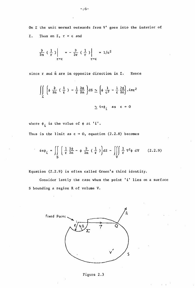
On L the unit mormal outwards from V' goes into the interior of

Eo Thus on l:. r = ~ and

a (1 ) 1 an r

() (1)1 ar r

r=(. r=(.

since r aud n are in opposite direction in L Hence

wllcre ~. is the value of • at 1

~ 4TI~. as ~.,. 0 - 1

, . , 1 •

Thus in the limit as ~ .,. 0, equation (2.2.8) becomes

4nq,. 1 ff[

s l. <;72. dV r

Equation (2.2.9) is often called Green's third identity.

(2.2.9)

Consider lastly the case when the point 'i' lies on a surface

S bounding a region R of volume V.

fixed

Q

, V 5

Figure 2.3

-37-

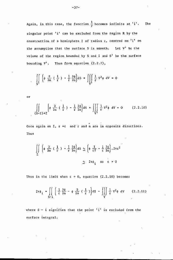
Again, in this case, the function ~ becomes infinite at r

,. , 1 •

singular point 'i' can be excluded from the region R by the

construction of a hemisphere E of radius E:, centred on 'i' on

the aS5umption that the surface 5 is smooth. Let V' be the

volume of the region bounded by 5 and Land 5' be the surface

bounding V' • Then from equation (2.2.7),

If (~ 5'

or

a ( 1 an r

1 01» ) - - - dS + r an fJJ

V'

.!. '7 21> dV = 0 r

The

If [1> a ( 1

dn r .!. '7 2 .p dV = 0 r

(2.2.10)

(5-E)+E

Once again on E, r =e: and'r and n are in opposite directions.

ThuR

~ 2.~. as £ ~ 0 1

Thus in the limit when £ + 0, equation (2.2.10) becomes

2'1> . 1 = If [

5-i fJf

V

.!. '7 21> dV r

(2.2.11)

where 5 - i signifies that the point 'i' 1S excluded from the

surface integral.

-38-

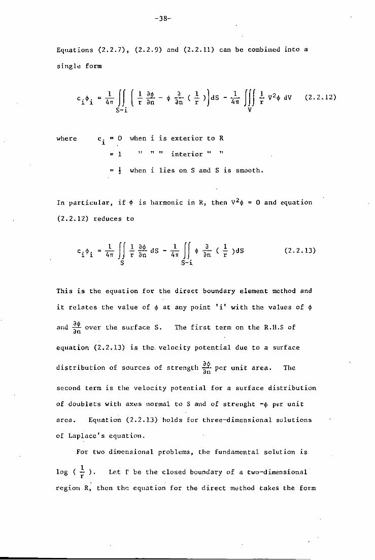
Equations (2.2.7), (2.2.!1) and (2.2.11) can be combined into a

single form

where

c.cj>. 1 1 4

ln If [ - 4

ln If f

s-i

c. = 0 Hhen i is exterior to R 1

= 1 11 "" interior If "

V

! when i lies on Sand S is smooth.

(2.2.12)

In particular, if <I> is harmonic 1n R, then V2cj> = 0 and equation

(2.2.12) reduces to

c.1>. 1 1 1 ff 4n

S

le 2.t dS - 1 If cj> r an 4n S-i

a (1 d an r) S (2.2.13)

This is the equation for the direct boundary element method and

it rclates the value of cj> at any point 'i' with the values of <P

and 2.t over the surface S. an

The first term on the R.H.S of

equation (2.2.13) is the. velocity potential due to a surface

distribution of sources of strength 41'- pcr unit area. The all

second term is the velocity potential for a surface distribution

of doublets with axes normal to S and of strenght -<I> per unit

area. Equation (2.2.13) holds for three-dimensional solutions

of Laplacc's equation.

For tHO dimensional problems, the fundamental solution is

log ( le ). r

Let r be the closed boundary of a two-dimensional

regi.oll R, then thoo equation for the direct method takes the form

= 1 J 2n r

where c. = 0 1

- 1

= !

-39-

1 a,' 1 log ( - ) = dr - -r an 2n

when i is exterior to

" " " interior "

when i lies on r and

J r-i

r

"

r is

4> a an

smooth.

(2.2.14)

If the unit normal vector n is drawn inwards to the domain,

then the equations for the direct method for three- and two-

dimensional problems can be written from equation (2.2.13) and

(2.2.14) by replacing n by -no

2.3 FORMULATION OF THE DIRECT BOUNDARY ELE~ffiNT ~THOD FOR

AN INFINITE DOMAIN

The equations for the direct boundary element method given

in section (2.2) were derived for a finite domain bounded by a

surface s. In problems of external vehicle aerodynamics, the

flow field is exterior to S, the surface of the vehicle, and is

considered to be of infinite extent.

I

S

R

Figure 2.4

- -----------------------------------------------------------------------------40-

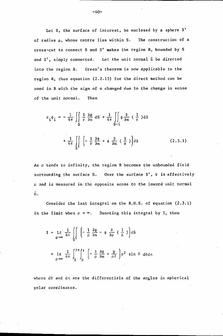
Let S, the surface of interest, be enclosed by a sphere S'

of radius p, whose centre lies within S. The construction of a

cross-cut to connect Sand S' makes the region R, bounded by S

and S', simply connected. Let the unit normal n be directed

into the region R. Green's theorem is now applicable to the

region R, thus equation (2.2.13) for the direct method can be

used in R with the sign of n changed due to the change in sense

of the unit normal. Then

ci~i = - 4l1T fJ ~*dS + 4l1T fJ ~aan (~)dS

+.1.-41T

S S-i

(2.3.1)

As p tends to infinity, the region R becomes the unbounded field

surrounding the surface S. Over the surface S', r is effectively

p and is measured in the opposite sense to the inward unit normal

n.

Consider the last integral on the R.H.S. of equation (2.3.1)

in the limit when p ->- 00. Denoting this integral by I, then

I 1 ff [- 1 a'" all Lt -- - - -'2 - ~ - ( - ) dS 411 p an ap p p.)oO:I Si

1 Lt 41T p--

1 aq, --+ p an sin e dOdn

where dO and dn are the differentials of the angles in spherical

polar coordinates.

-41-

_ This integral must remain bounded in the limit p + ~,

which imposes a restraint upon the possible form $ can take as

In general there will be either no flow at infinity,

hence $ is constant, say $ , or else a steaming flow in, say, .,

the negative x direction, which would imply that

$ = Ux + $., (2.3.2)

where $ is the velocity potential of the uniform stream.

Clearly the former case is a particular instance of the latter

(U = 0).

Now in spherical polar coordinates

x p sin e cos n

Therefore equation (2.3.2) becomes

$ = Up sin e cos n + $.,

~-an - ~ - -U sin e cos n . ap -

1 I = Lt 4"

p-

1 = Lt 4n

p-

n+sin e(Up sin

-42-

= ~O'J

!lcnce equation (2.3.1) takes the form

c.$. = 1 1

1 $"" - 4 .. ff .!:. .£.t d5

r an S

+ 41 .. If $

5-i

a (.!:. )dS an r (2.3.3)

t This equation is the st"f'ment of the direct boundary element

method for regions of infinite domain.

For two-dimensional problems, the equation of the direct

boundary element method for an infinite domain takes the form

c.$ . 1 1

1 = 'Pee - 2IT f log ( .!:. ) .£.t df

r an f

+...!..f$ 2-.

f-i

2.4 DERIVATION OF THE EQUATION FOR THE INDIRECT BOUNDARY

ELENENT METHOD

(2.3.4)

Frequently the boundary element method is implemented via

the application of a distribution of sources and/or doublets Oll

the boundary and the problem is then solved in terms of the

unknown strengths of the sources or doublets. This technique is

called the indirect method and can be derived from the equation

of the direct boundary element method.

-43-

R

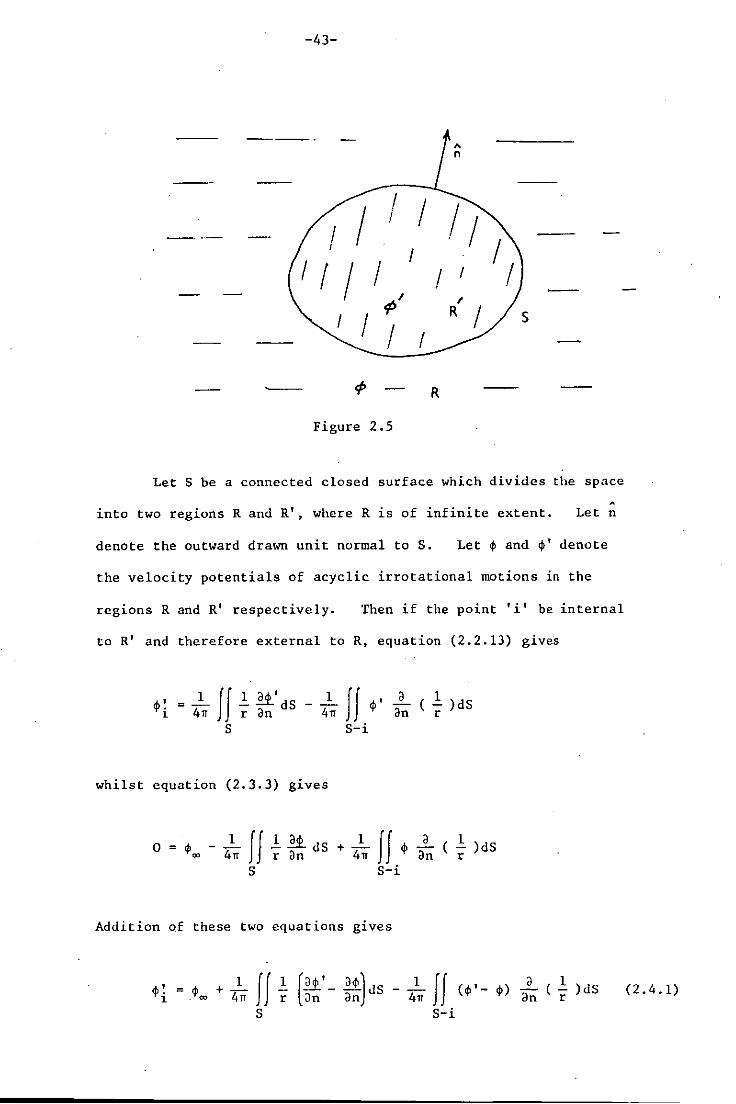
Figure 2.5

Let S be a connected closed surface which divides the space .

into two regions Rand R', where R is of infinite extent. Let n

denote the outward drawn unit normal to S. Let $ and $' denote

the velocity potentials of acyclic irrotational motions in the

regions Rand R' respectively. Then if the point 'i' be internal

to R' and therefore external to R, equation (2.2.13) gives

$! = ~ II ~ lt'dS 1 411 r an 1 II ~, - 4iT ~

S S-i

whilst equation (2.3.3) gives

~ lt <IS + ~ r an 4n

Addition of these two equations gives

a (~) dS an r

a (~)<lS an r

a (~) dS an r (2.4.1)

-44-

Similarly in the case when 'i' is internal to R and hence external

to R', the same equation results with $. replacing $~ on the L.H.S. 1 1

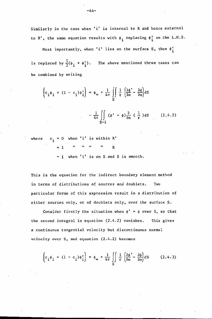
Most importantly, when 'i' lies on the surface S, then $~ 1

is replaced by -21($' + $~). The above mentioned three cases can

1 1

be combined by writing

where

[c. $. + (1 - c.) $ ~) = 11 1. 1.

1 [It' - It] dS r an an s

4~ If ( ~' _ ~,a (.!:.) dS 't' 't'Jafi r

S-i

c. = 0 when 'i' is within RI 1

= 1 " " " " R

I when 'i' is on Sand S 1S smooth.

(2.4.2)

This is the equation for the indirect boundary element method

in terms of distributions of sources and doublets. Two

particular forms of this expression result in a distribution of

either sources only, or of doublets only, over the surface S.

Consider firstly the situation when $' = $ over S, so that

the second integral in equation (2.4.2) vanishes. This gives

a continuous tangential velocity but discontinuous normal

velocity over S, and equation (2.4.2) becomes

1 [It' - It]dS r an an (2.4.3)

-:-45-

for all positions of , . ,

1 • The motion is that due to a surface

distribution of sources of strength [~' - a~) per unit area. an an

This is the form of the indirect boundary element method in

terms of sources alone.

Secondly suppose that a~' _a~ - - over the surface S. an - an The

first integral in equation (2.4.2) now vanishes and it reduces

to

[c .•. + (1 - c.).!) 1 1 1 1

(.' - .)~ ( ! )dS an r (2.4.4)

There is now continuous normal velocity but discontinuous

tangential velocity over the surface S, which implies that the

motion is due to a surface distribution of doublets of strength

- (.' - .) per unit area, with axes normal to S. Equation

(2.4.4) is the indirect formulation of the boundary element

method in terms of doublets alone. It may be shown (Lamb [23])

that the representations (2.4.3) and (2.4.4) are unique, whereas

the representation (2.4.2) is not unique.

Of the infinitely many possible formulations of combined

source and doublet distributions, one war"thy of special note is

the case when the interior flow potential ~' = o. Equation

(2.4.2) then reduces to equation (2.3.3), establishing the formal

equivalence of the direct and indirect methods.

-46-

SECTION 3

DISCRETE ELEMENT FOR~lULATION OF THE

aOUNDARY INTEGRAL EQUATION

3.1 INTRODUCTION

The equation (2.2.13) for the direct boundary element method

cannot usually be solved analytically and recourse is made to

numerical methods. Since this equation involves integrals to be

evaluated at the surface of the body under consideration, the

surface of the body is divided into a large number of boundary

elements and the integral over the surface is then replaced by

the sum of the integrals taken over all the elements. The

boundary integral equation thus reduces to a set of simultaneous

linear algebraic equations, which can be solved by simple

numerical methods.

The following sections outline the various procedures which

can be followed for element discretization, matrix formulation,

integration over an element and solution of the resultant set

of equations.

-47-

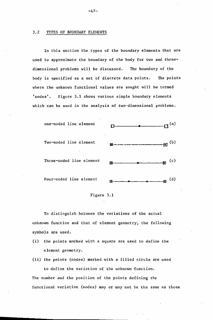
3. 2 TYPES OF BOUNDARY ELEHENTS

In this section the types of the boundary elements that are

used to approximate the boundary of the body for two and three-

dimensional problems will be discussed. The boundary of the

body is specified as a set of discrete data points. The points

where the unknown functional values are sought will be termed

'nodes'. Figure 3.1 shows various simple boundary elements

which can be used in the analysis of two-dimensional problems.

one-noded line element D~ ______ ~. ______ ~[](a)

Two-noded line element 19---------------8 (b)

Three-noded line element 8'--------..... -------,8 (c)

Four-noded line element 131----... ---... ---El (d)

Figure 3.1

To distinguish bet,,,een the variations of the actual

unknown function and that of element geometry, the following

symbols are used.

(i) the points marked with a square are used to define the

element geometry.

(ii) the points (nodes) marked with a filled circle are used

to define the variation of the unknown function.

The number and the position of the points defining the

functional variation (nodes) mayor may not be the same as those

-48-

of the points defining the element geometry. In figure 3.1

the geometry of the element in each case is defined by the two

end points while the functional variation is defined by onc, two,

three and four nodes in (a), (b), (c) and (d) respectively.

The interpolation functions or 'shape functions', for the

functional variation over the elements in (b), (c) and (d) are

discussed in Hucbner (27) and are given as follows:

For the two-noded line element shown in figure 3.1 (b), the

shape functions in terms of the local coordinate ~ are

NdO = \(l-~), Nz(O = \(1+0, -l:;~:;l (3.2.1)

the origin being at the centroid of the element.

For the· three-noded line element shown in figure 3.1 (c), the

shape functions are

(3.2.2)

and for the four-noded line element shown in figure 3.1(d), the

shape functions are

(3.2.3)

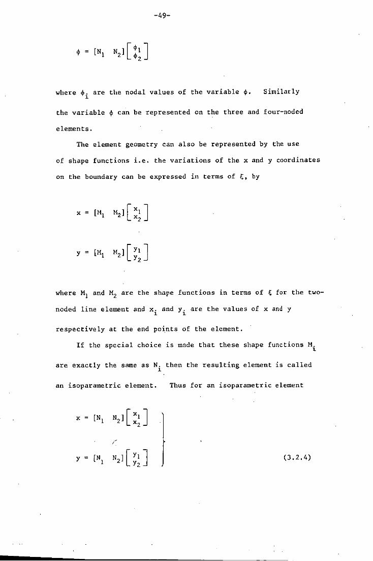
Any variable cP defined on the two-noded element say, can

then be approximated by

-49-

N 1 [~l ] 2 ~2

where .p. are the nodal values of the variable ~. 1

Similarly

the variable .p can be represented on the three and four-noded

elements.

The element geometry can also be represented by the use

of shape functions i.e. the variations of the x and y coordinates

on the boundary can be expressed in terms of 1;, by

where MI and M2 are the shape functions in terms of 1; for the two-

noded line element and x. and y. are the values of x and y 1 1

respectively at the end points of the element.

If the special choice is made that these shape functions M. 1

are exactly the same as N. then the resulting element is called 1

an isoparametric element. Thus for an isoparametric element

x [NI N21[:~J 1

/

I

J y = [NI N21[~~J (3.2.4)

-50-

The element shown in figure 3.l(b) is isoparametric since the

same points define the geometry as well as the functional

variation.

If the number of nodes defining the functional variation is

less than that used to define the geometry, then the element is

called super-parametric. Thus the element shown in figure 3.1(a)

is super-parametric, noting that the variation of geometry is

more general than that of the actual unknown. Similarly if the

number of nodes used to define the variation of the unknown is

greater than that used to define the geometry, then the resulting

element is called sub-parametric. The elements shown in (c)

and (d) of figure 3.1 are sub-parametric.

The functional variation shown in (a), (b), (c) and (d) of

figure 3.1 is termed constant, linear, quadratic and cubic

respectively.

For three dimensional problems, the boundary elements are

part of the external surface of the body. They are usually

of two types, either quadrilateral or triangular elements.

In boundary element or finite element work there is a tendency

to prefer quadrilateral elements, which will be used exclusively

1n this thesis. Figure 3.2 shows different types of

quadrilateral elements used for three dimensional problems.

-51-

•

(b)

(c) Figure 3.2 (d)

k In figure 3.2 the geometry ofLquadrilateral element in each case

is defined by four corner points while the functional variation

is defined by one, four, eight and twelve nodes in (a), (b), (c)

and (d) respectively. The functional variation in (a), (b), (c)

and (d) of figure 3.2 is termed constant, linear, quadratic and

cubic respectively. The elements shown in (a) and (b) of figure

3.2 are superparametric and isoparametric respectively while the

elements in (c) and (d) are sub-parametric.

The shape functions for the functional variation over the

elements shown in (b), (c) and (d) of figure 3.2 are discussed

in Zienkiewicz [28] and are given as follows:

For the element shown in figure 3.2(b), the shape functions

in terms of the local coordinates ~ and n are

-52-

(3.2.5)

where (~k' nk

) are the coordinates of the kth node.

For the element shown in figure 3.2(c), the shape functions are:

Corner nodes:

Typical midside node: ~ = 0, n = + 1 "k -

where (~k' nk) are the coordinates of the kth node.

(3.2.6)

For the element shown in figure 3.2(d), the shape functions

are:

Corner nodes:

Typical midside node: ~k 1

± "3

where (sk' nk) are the coordinates of the kth node.

(3.2.7)

The boundary elements considered so far in figures 3.1 and

3.2 have been of linear geometrical variation only; in problems

where the boundary is curved, the true boundary shape can be

modelled more precisely for a given number of elements by using

-53-

higher order shape functions for the geometrical variation.

Curved boundary elements for two and three-dimensional

problems can be obtained by transforming the standard regions

shown in (a) and (b), respectively, of figure 3.3.

,.,

+1

~------------~-7)J -I 0 +1 -I 0

< a) -I

( b) Figure 3.3

Figure 3.4 shows some two and three-dimensional curved boundary

elements.

•

(a) (b)

(c) (d)

+1

-54-

Each of the elements shown in figure 3.4 is isoparametric since

the same points define the element geometry as well as the

functional variation. The elements shown in (a) and (b) of

fi.gure 3.1 will be termed the constant and linear boundary

elements and those shown in (a) and (b) of figure 3.4 as the

quadratic and cubic boundary elements for the two-dimensional

problems. Similarly the elements shown in (a) and (b) of figure

3.2 and those shOw"Il in (c) and (d) of figure 3.4 will be termed

the constant, linear, quadratic and cubic boundary elements

respectively, for the three-dimensional problems.

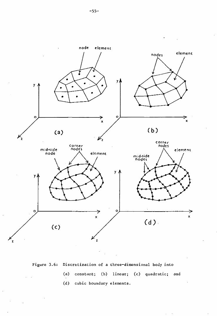
Figure 3.5 shows a two-dimensional body discretized into

constant, linear and quadratic boundary elements, while figure

3.6 shows a three-dimensional body discretized into constant

linear, quadratic and cubic boundary elements.

y y

~ment

0 )x 0

(a)

extreme nodes

%ement

( b) x

mid-node y J

Figure 3.5: Discrctization of a ~Iement

two-dimensional body into

(a) constant;

(b) linear and

(c) quadratic boundary elements. ,. 0 x

(C)

-55-

node element

element

y y

0)-________________________ '" o)-______________________ ~

x x

(a) (b)

z

element

y y

o)---------------------~ o)-______________________ ~~

x x

Cc) (d)

z z

Figure 3.6: Discretization of a three-dimensional body into

(a) constant; (b) linear; (c) quadratic; and

(d) cubic boundary elements.

-56-

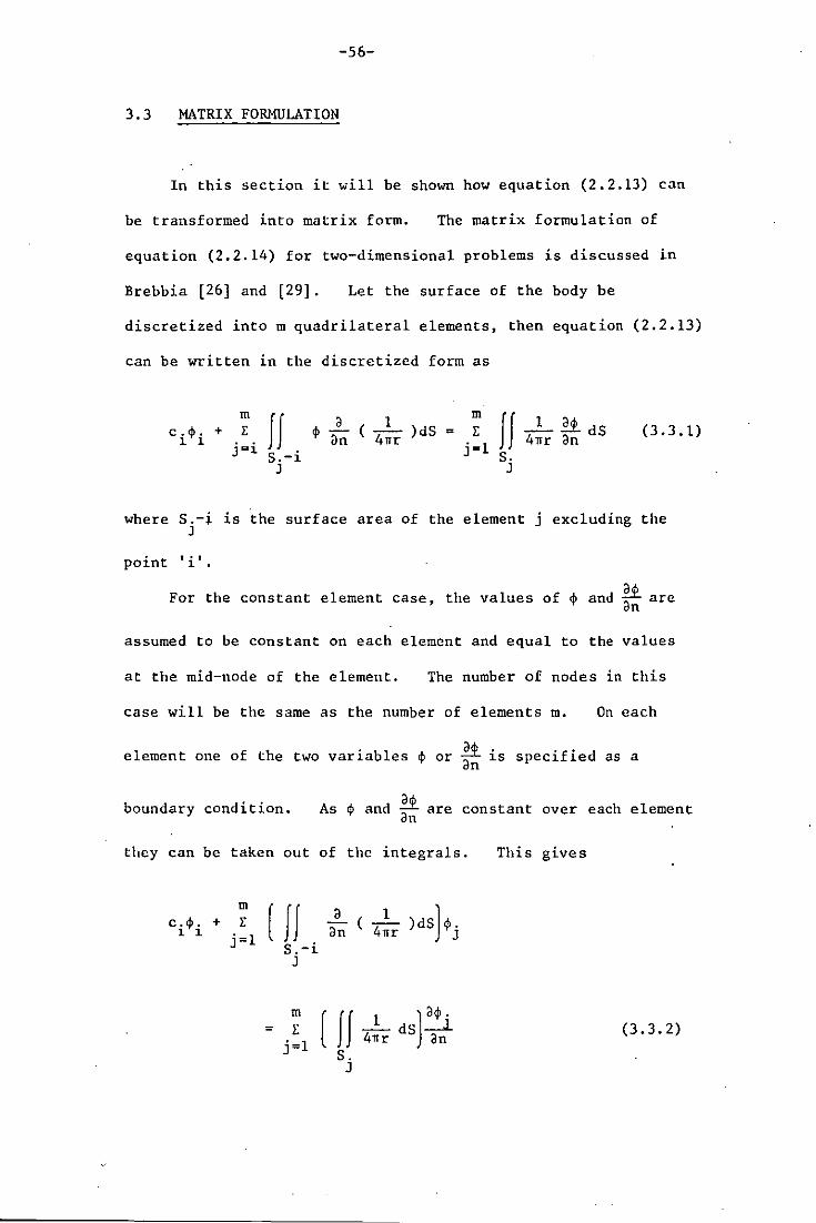
3.3 MATRIX FORMULATION

In this section it will be shown how equation (2.2.13) can

be transformed into matrix form. The matrix formulation of

equation (2.2.14) for two-dimensional problems is discussed in

Brebbia [26] and [29]. Let the surface of the body be

discretized into m quadrilateral elements, then equation (2.2.13)

can be written in the discretized form as

c . q,. + 1 1

m 1:

j=i If. S.-1

J

II _1_ 2i dS 4nr an

S. J

(3.3.1)

where s.-i is the surface area of the element j excluding the J

point t • t 1 •

For the constant element case, the values of q, and * are

assumed to be constant on each element and equal to the values

at the mid-node of the element. The number of nodes in this

Case will be the same as the number of elements m. On each

element one of the two variables q, or * is specified as a

boundary condition. As q, and :: are constant over each element

they can be taken out of the integrals. This gives

c.<j>. + 1 1

m

1: j=l

(If S.-i

J

m = E

j=l ( II _1 dS)~

4nr an (3.3.2)

S. J

-57-

Equation (3.3.2) applies for a particular node 'i' and the integrals

If a 1 an ( 4nr )dS relate the node 'i' with the element 'j' over

S.-i J

which integrals are evaluated. These integrals will be denoted

by H ..• 1J

The integrals on the R.H.S. are of the type

If ( 4!r )dS s.

J

and will be denoted by G ..• 1J

can be written as

c.<p. + 1 1

m E

j=l H .. <p. =

1J J

m E

j=l G •.

1J

Hence equation (3.3.2)

(3.3.3)

The integrals H .. and G .. in equation (3.3.3) are difficult 1J 1J

to evaluate analytically and are usually evaluated numerically.

Morino, Chen, and Suciu [11] have obtained approximate analytical

solutions of these integrals for quadrilateral elements with

constant functional value and linear geometrical variation, but

the integrals become more difficult for higher order elements.

In this thesis, the integrals over the quadrilateral elements

will be calculated numerically.

1 H .. when

Let H .. = 1J 1J H .. + c. when

1J 1

Equation (3.3.3) can be rewritten as

m E

j=l H .. <p.

1J J

m E

j=l G . .

1J

i " j (3.3.4) i = j

(3.3.5)

-58-

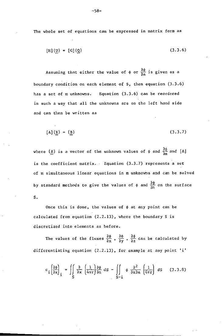
TIle whole set of equations can be expressed in matrix form as

(3.3.6)

Assuming that either the value of q, or it is g.ven as a an

boundary condition on each element of S, then equation (3.3.6)

has a set of m unknowns. Equation (3.3.6) can be reordered

in such a way that all the unknowns are on the left hand side

and can then be written as

{B} (3.3.7)

where {X} is a vector of the unknown values of ~ and ~~ and lA]

is the coefficient matrix. Equation (3.3.7) represents a sct

of m simultaneous linear equations in m unknowns and can be solved

by standard methods to give the values of q, and ~ on the surface

S.

Once this is done, the values of q, at any point can be

calculated from equation (2.2.13), where the boundary S is

discretized into elements as before.

The values of the fluxes * ' * ' ~: can be calculated by

differentiating equation (2.2.13), for example at any point 'i'

[_l_)it dS -4nr Cln If [ 1 ) dS

lmr (3.3.8)

S-i

-59-

Thus far the matrix formulation has been restricted to the

simple case for which ~ and ~! are constant over each element.

Consider next a surface which is divided into m linear, quadratic

or cubic quadrilateral elements i.e. quadrilaterals with four,

eight or twelve nodes. In this case the number of nodes will be

more than the number of elements. Suppose that M is the number

of nodes in this case. Using the shape functions as defined in

equation (3.2.5) or (3.2.6) or (3.2.7), ~ and ~! can be written as

.£t (I;, n) = an L l.:

k=l

where L denotes the number of nodes on each element.

The integrals along the element' j' on the L.ll.S of equation

(3.3.1) can now be written as

If S.-i

J

a cj> an [ 1 ) dS = JfJ 41rr

S.-i J

l.: N a 1 dS ( L ) ( ) k=l k cj>k an 4Tfr

~L

where

=

k h ..

1J

( I h ..

1J

=JJ s.-i

J

2 h ..

1J

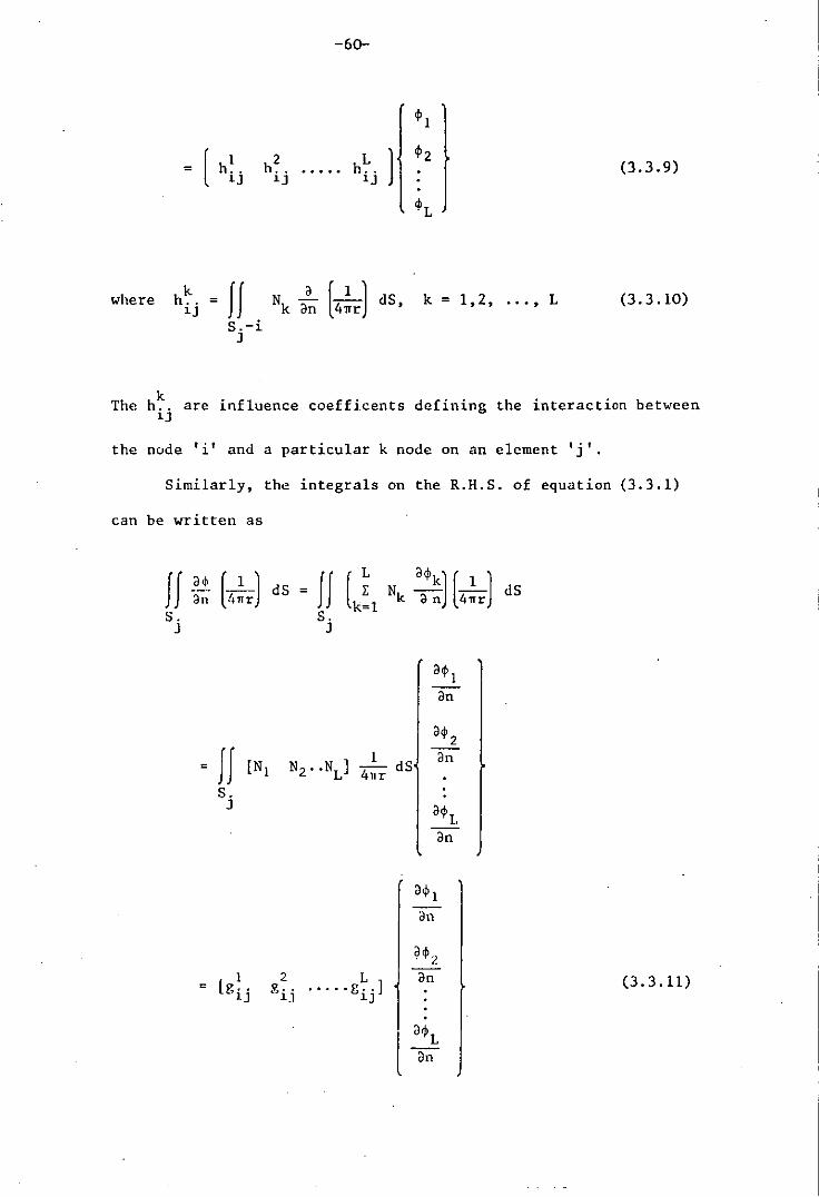
-60-

<PI

L ) <P2 (3.3.9) h ..

1J

4>L

(4!r) dS, k=1,2, ... ,L (3.3.10)

The h~. are influence coefficents defining the interaction between 1J

the node 'i' and a particular k node on an element 'j'.

Similarly, the integrals on the R.H.S. of equation (3.3.1)

can be written as

II od.! (.2_) d S 3n 4nr

= If [~ N d<1>k) [_1 ) dS k=l k d n 41Tr

S. J

= JJ [NI

S. J

I [g .. 1J

S. J

a<P I an

a<p 2

N2 • .NLl _1_ dS an 4nr

2 I. g ....... g .. ]

1J 1J

a.pI.

an

l a.pL

an

(3.3.11)

-61-

where k

g .. 1J

k=1,2, ..... ,L (3.3.12)

To write equation (3.3.1) corresponding to the node 'i',

the contributions from all of the elements associated with the node

'i' are to be added into one term, defining the nodal coefficients.

This will give the following equation:

(3.3.13)

. where each H .. and G .. term is the sum of the contributions from

1J 1J

all the adjoining elements of the node , .,

1 • Hence equation

(3.3.13) represents the assembled equation for node 'i' and can

be written as·

c.<j>. + 1 1

or

H E

5=1

M E

j=l

H .. q,. = 1J J

H .. $. = 1J J

M E

j=l

M E

j=l

G •. 1J

G .. 1J

act> • _J an

(3.3.14)

-62-

where

r .

i ,;, j H .. for 1J

H .. =

t (3.3.15)

1J H .• + c. for i = j 1J 1

When all the H nodes are taken into consideration, equation

(3.3.14) produces an H x H system of equations which can be

written in matrix form as

[H) {.!!} [G) {g) (3.3.16)

which is of the same form as equation (3.3.6). This set of

equations can then be rearranged and solved in the same manner·

as outlined previously.

In general the surface will not be smooth at the point ,. , 1 ,

such that c. ,;, ! in equation (3.3.15). 1

One can, however, calculate

the diagonal terms of [H) by using the fact that when a uniform

potential is applied over the whole boundary, including that at

infinity, there will be no flux of ~ through the surface at any

point. Thus equation (3.3.16) becomes

[H) {.!!} {O} (3.3.17)

Equation (3.3.17) indicates that the sum of all the terms of [Hl

in a row must be zero, hence the values of the coefficients in a

diagonal can easily be calculated once the off-diagonal coefficients

are all known, as

-63-

H H •. = - E H •. (3.3.18)

11 J=f 1J (J ,,<")

Thus for the matrix formulation of the equation (2.2.13),

which holds for an interior domain has been considered. For

exterior flow problems, equation (2.3.3) for the direct method

can be written as

M M a$ . E H .. $ . + $"" E G •• _J (3.3.19)

j=l 1J J j=l lJ an

1 H .. when i f. j

1J where H •• = (3.3.20)

lJ 11 .. -c. when i = j 1J 1

following the same method outlined previously.

When all the nodes are taken into consideration, equation

(3.3.19) produces an H x (M + 1) system of equations which can

again be put in the matrix form as

[II]{~} = [G] {Sl} (3.3.21)

Note that now {u} in equation (3.3.21) has (H + 1) unknowns

To solve precisely this system of

equations, the value of $ at some position must be specified.

For convenience, if> is chosen as zero. ""

Thus the M x (M + 1) system

reduces to an M x H system of equations which can be solved as

before, but now the diagonal coefficents of [H] will be found by

1I.. = 11

M E (H .. - 1

J=, 1J (ji' <)

.!

(3.3.22)

-64-

3.4 EVALUATION OF INTEGRALS

The integrals in equations (3.3.10) and (3.3.12) are difficult

to evaluate analytically, therefore their numerical evaluation will

be considered in this section. Since these integrals involve

shape functions which depend upon the local coordinates I; and n

defined on the standard element shown in figure 3.3, it is required

to find the transformation from the cartesian x, y, z system to

the 1;, n, ~ system defined over the body.

z

-R

o y

x Figure 3.7

Following Brebbia [26) or Zienkiewicz [28), consider the systems

defined in the figure 3.7. For a function u, the general

transformation is given by

-65-

au au ax + ~E.Y. +

au az -=-- az~ a~ ax a~ ay a~

au = au ax + ~E.Y. +

au az -- --a~ ax a~ ay all az a~

au au ax +

;)u E.Y. +

au az ~=ax~

-_.-ay ai; az a,

which can be put in the matrix form as

au ax ~ az au at; a~ a~ a~ ax

au ax E.Y. az au =

a~ a~ aT] aT] ay

au ax ~ az au a~ a~ a~ a~ az

au au a~ ax

au = J au or aT] ay

au au a~ az

where J denotes the 3 x 3 matrix in the above equation. Thus

the inverse relationship can be found as

'" I au ax a~

au rl au

" I = aT]

au ~ az a~

-66-

4

Replacing u by R for instance, the differential of area (such

as dS) can be defined as

dS

Since iI: =

and x =

I ail: ail: ~xan

, xi + yj + zk

x(~, n, ~)

y = y(~, n, ~)

z =

ail: - = a~

=

=

Similarly

and

z(~, n,

ail: ax --ax a~

ax • ~1

ail: a~

( ax ~'

=

=

~)

ail: 2.1. + ay a~

+ 2.1.. aE; J +

2.1. ~) aE; , aE;

[ax an'

(ax ~'

ail: az + --az a~

~« aE;

Note that Icl is the magnitude of the normal vector,

+ -> + + aR aR aR n =

~ = ~xan

= (g!, g2' g3)

(3.4.1)

(3.1 •. 2)

-67-

where gl =

=

=

and = + g~ + (3.4.3)

Using these relationships, the integrals in equations

(3.3.10) and (3.3.12) over the linear quadrilateral elements

become

k .( ( a ( 4!r ) IGld~dn, k 1,2, ... ,L (3.4.4) h .. = Nk an =

1J _1 _1

and k

( ( Nk ( 4!r ) IGld~dn, k = 1,2, •.• ,L (3.4.5) g .. = 1J

-1 -1

The integral in equation (3.4.4) and (3.4.5) are now on the

standard element -1 ~ ~ ~ 1, -1 ~ n ~ 1, as shown in figure

3.3 (b), which can then be evaluated using two-dimension",l Gaussian

quadrature, which approximates a definite integral by summation

over a finite number of points. Thus one can write

1 1 I I f(~, l1)d~dl1 '" _1 _1

P

E Wp f(~p' np) p=l

(3.4.6)

-68-

where Ware the weighting coefficients and (~ , n ) are the p . p p

coordinates of the associa~ed P Gaussian points. Thus the

region of integration for the Gaussian quadrature is precisely

the same as the standard element, namely -1 ~ ~ ~ 1, -1 ~ n ~ 1.

Equation (3.4.4) and (3.4.5) can be written as

k h .. ' = ~J

k g .. ~J

p - 2.. E

. 411 1 p=

1 P 41T E

p=l

(3.4.7)

(3.4.8)

Now r is the distance from the fixed point 'i' to any general

point Q(x ,y z) on the surface of the body under consideration. q q' q

->-r = +

"'"

(y - y.)j q ~

+ (z - z.)k q 1

and for Lisoparamctric quadrilateral element,

x q

=

z = q

(3.4.9)

(3.4.10)

Thus n.r can be found from equation (3.4.2), (J.4.9) and (3.4.10).

-69-

In general Gauss-quadrature formulae give good results,

but not when the singularity is present on the element over which

the integration is being performed. In such cases alternative

numerical quadrature schemes have been developed. For three-

dimensional problems, a modified quadrature rule for this case is

discussed in section (6). In two-dimensional formulations for

this case, either a higher order integration rule or a special

logarithmically weighted integration formula, Stroud and Secrest

[30], should be used.

3.5 SOLUTION OF THE SYSTEN OF EQUATIONS

When the boundary integral equation (2.2.13) is transformed

into a system of linear algebraic equations (3.3.7), then the

solution of this system is an important part of the total

calculation. The system of equations (3.3.7) will be solved

using the G~uss elimination method as well as the Gauss-seidel

method. The detailed discussion of these methods can be seen

from many texts e.g. Nobel and Daniel [31]. Only a brief

comparison of these two methods will be presented here.

G",uss elimination works for any non-singular system of H

equation in M unknowns, while the Gauss-Seidel method works for

only specific cases where convergence occurs. In situations

where convergence does occur for the Gauss-Seidel method, the

choice between using this or Gauss elimination depends upon

several factors, in particular the system size of the equations H.

This is because the number of arithmetic operations required for

-70-

the Gauss elimination method to solve a system of M linear equations

is proportional to M3, and the number of operations for one

iteration of the G~ss-Seidel method is proportional to M2.

Thus if the Ga-uss-Seidel metl10d converges in fewer than M

iterations, it is computationally more efficient than Gauss

elimination. The speed of convergence depends upon the precise

format of the coefficients of the equation, as well as the guessed

starting values for iteration. In general, the larger the

system size M is, the more likely it is that Ga.-lLss-Seidel will

require less computing time than Gauss elimination. Furthermore

the round-off error for the Gauss-Seidel is generally smaller than

that for Ga.-~ss elimination. Finally, when M is very large, then

the storage of M2 entries of the coefficient matrix [AJ on the

computer becomes a problem. It then becomes necessary to store

the coefficients on disc and read them into the program line by

line for solution of the equations. The Gauss-Seidel method is

much more convenient for line by line solution than Gauss

elimination. Comparison of the Gauss-Seidel and Gauss elimination

methods of solution for problems of three-dimensional exterior

unbounded flows is given in section (4).

-71-

SECTION 4

A DIRECT BOUNDARY ELEMENT METHOD APPLIED

TO POTENTIAL FLOW PROBLEMS

4.1 INTRODUCTION

In this section the direct boundary element method is applied to

obtain the potential flow solution around two and three-dimensional

bodies, for which analytical solutions are available. To check the

accuracy of the method, the calculated flow velocities or the pressure

distributions are compared·with the analytical solutions for flows

over the surfaces of a sphere and ellipsoids of revolution in the

three- dimensional case, and over the boundary of a circular cylinder

in the two-dimensional case.

Since the flow field around a body lying in the proximity of the

ground is different from the flowfield around the same body when it is

lying in an unbounded space, the ground plane problem is an important

feature which is also discussed in this section.

A further feature of the real flow field about a bluff road

vehicle is the presence of a wake downstream of the body. A method of

accounting for this feature in the potential flow model is presented at

the end of this section.

-72-

4.2 UNBOUNDED FLOW FIELD CALCULATIONS

Consideration is given firstly to the uniform streaming flow about

a circular cylinder, a sphere and ellipsoids of revolution. In the

case of a sphere and ovary ellipsoids, the surface of the body under

consideration is discretized into linear isoparametric quadrilateral

elements and the integrals over each element have been evaluated

numerically using Gauss-quadrature with four integration points. In

the case of a circular cylinder, the boundary of the cylinder is

discretized into constant and linear boundary elements and the inte9Y~(~'

over 'these elements,are calculated numerically using Gauss-quadrature

with four integration points except for the element corresponding to

the node under consideration.

calculated analytically.

For this element the integrals are

4.2.1 FLOW PAST A CIRCULAR CYLINDER

Boundary element methods can be used to solve two-dimensional

interior or exterior flow problems. As an example of an exterior

flow problem, consider the flow past a circular cylinder. Let a

circular cylinder be of radius 'a' with centre at the origin and let

the onset flow be the uniform stream with velocity U in the positive

direction of the x-axis as shown in figure 4.1.

-73-

y

)

)

u ) x

)

,

Figure 4.1

The magnitude of the exact velocity distribution over the boundary of

the circular cylinder is given in Milne-Thomson [24) as

.... IVI = 2aU sin e (4.2.1.1)

where e is the angle between the radius vector and the positive

direction of the x-axis.

Now the condition to be satisfied on the boundary of the circular

cylinder is

. ... n.V = 0 (4.2.1.2)

where n is the unit normal vector to the boundary of the cylinder.

Since the motion is irrotational,

... V = -17~

where ~ is the total velocity potential. Thus equation (4.2.1.2)

becomes

or

n. (-\701» = 0

a 01> 0 an =

-74-

(4.2.1.3)

Now the total velocity potential 01> is the sum of the perturbation

velocity potential $ and the velocity potential of the uniform c.c

stream $ u.s

i.e.

or a$ .

c.c an

which on using equation (4.2.1.3) becomes

=

(4.2.1.4)

(4.2.1.5)

But the velocity potential of the uniform stream. given in Milne-

Thomson [241. is

= -U ax an

= -U(n. i)

Thus from equations (4.2.1.5) and (4.2.1.7).

= U(n.i)

(4.2.1.6)

(4.2.1.7)

(4.2.1.8)

-75-

or u --;::;;::x==;;: Ix2 + y2

(4.2.1.9)

Equation (4.2.1.9) is the boundary condition which must be satisfied

over the boundary of the circular cylinder.

Now for the approximation of the boundary of the circular cylinder,

the coordinates of the extreme points of the boundary elements can be

generated within the computer program as follows:

Divide the boundary of the circular cylinder into m elements in the

clockwise direction by using the formula

6k

~ [(m + 3) - 2k]1T/m, k ~ 1, 2, ••••• , m (4.2.1.10)

Then the coordinates of the extreme points of these m elements are

calculated from

k = 1, 2, ..... , m (4.2.1.11)

Take m ~ 8 and a ~ 1.

First consider the case of constant boundary elements where there

is only one node at the middle of the element and the potential cp, and

h . 1 d· . acp h d t e potent1a er1vat1ve an are constant over eac element an equal to

the value at the middle node of the element.

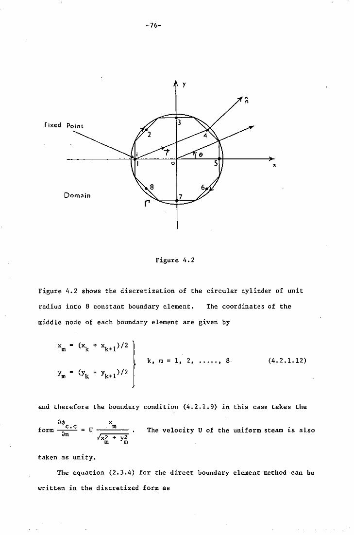
fixed Point

Domain

-76-

y

o

7

Figure 4.2

" n

x

Figure 4.2 shows the discretization of the circular cylinder of unit

radius into 8 constant boundary element. The coordinates of the

middle node of each boundary element are given by

k, m = 1, 2, ••••. , 8· (4.2.1.12)

and therefore the boundary condition (4.2.1.9) in this case takes the

a.p c. c x form U

m The velocity U of the uniform steam is also = an (x2 + y2

m m

taken as unity.

The equation (2.3.4) for the direct boundary element method can be

written in the discretized form as

-c.4>. + 1 1

-77-

m 1:

j=l U._ia~(2~ log ~)dr}j + 4>",

m = 1:

j=l

J

[f r.

J

(4.2.1.13)

The integrals in equation (4.2.1.13) on the elements can be calculated

numerically except the element on which the fixed point 'i' is located.

For this element the integrals are calculated analytically. Denoting

the integrals on the L.H.S. of equation (4.2.1.13) by H .. and that on 1.J

the R.H.S. by G .. , then 1J

H .. 1J = J a~Urr log '!')dr , r

r .-i J

1 = - 21T f .!. ~ dr

r an r.-i

J

= - 2lrr 11 _1

1 •• 9, r (n.r) "2 d~

where ~ is the length of the element r .. J

(4.2.1.14)

To find n.r let the coordinates of the fixed point 'i' be (x., y.) and 1 1

that of the variable point 'Q' be (x , y ), then q q

r = I(x - x.)Z + (y _ y.)Z • q 1 q 1

But Xq and yq in 'terms of ~ and the global coordinates ~ and Yk can be

written as

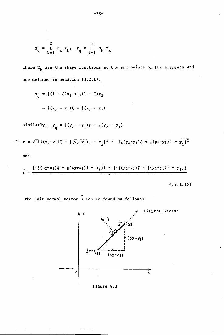
x = q Y = q

-78-

2 E

k=l

where Nk are the shape functions at the end points of the elements and

are defined in equation (3.2.1).

and

A

[{I(X2-Xl)~ + !(X2+Xl)} - xili + [{!(Y2-Yl)~ + !(Y2+Yl)} - Yi1j r =

r

(4.2.1.15)

The unit normal vector n can be found as follows:

y tangent vec tor

o x

Figure 4.3

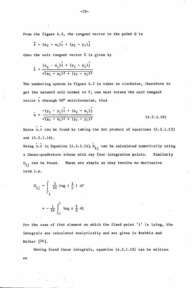
-79-

From the figure 4.3, the tangent vector to the point Q is

then the unit tangent vector t is given by

t (x2 - x1)i + (Y2 - Yl)j

I(X2 - xl)2 + (Y2 - YI)2

The numbering system in figure 4.2 is taken as clockwise, therefore to

get the outward unit normal to r, one must rotate the unit tangent

vector t through 900 anticlockwise, thus

n = -(Y2 - YI)i + (x2 - xl)j

I(X2 - xI)2 + (Y2 - YI)2 (4.2.1.16)

Hence n.r can be found by taking the dot product of equations (4.2.1.15)

and (4.2.1.16).

Using n.r in Equation (4.2.1.14), H .. can be calculated numerically using 1J

a Gauss-quadrature scheme with say four integration points. Similarly

G .. can be found. 1J

These are simple as they' involve no derivative

term i.e.

J 1 ( .!. ) G .. = - log dr

1J 211 r r.

1

1

= - 2111 J log r !:. d~ 2

-I

For the case of that element on which the fixed point 'i' is lying. the

integrals are calculated analytically and are given in Brebbia and

Walker [26].

Having found these integrals, equation (4.2.1.13) can be written

as

-c.$. + 1 1

Defining

H .. = 1J

-80-

m E

j=l H .• $. + $

1J J W

Pi' when

H •• - c. when 1J 1

=

i

i

m E

j=l

" j j

Equation (4.2.1.17) takes the form

m E

j=l H .• $. + $

1J J W =

m E

j=l G •.

1J

G .• 1J

a$ . _J

an

which can be expressed in matrix form as

[H]{.!!} = [G]{g)

(4.2.1.l7)

(4.2.1.18)

Since ~ is specified at each node of the element, the values of the

perturbation velocity potential $ are found at each node on the boundary

via equation (4.2.1.18). The total potential ~ is then found from

equation (4.2.1.4) which will then be used to calculate the velocity

on the circular cylinder. y

x

Figure 4.4

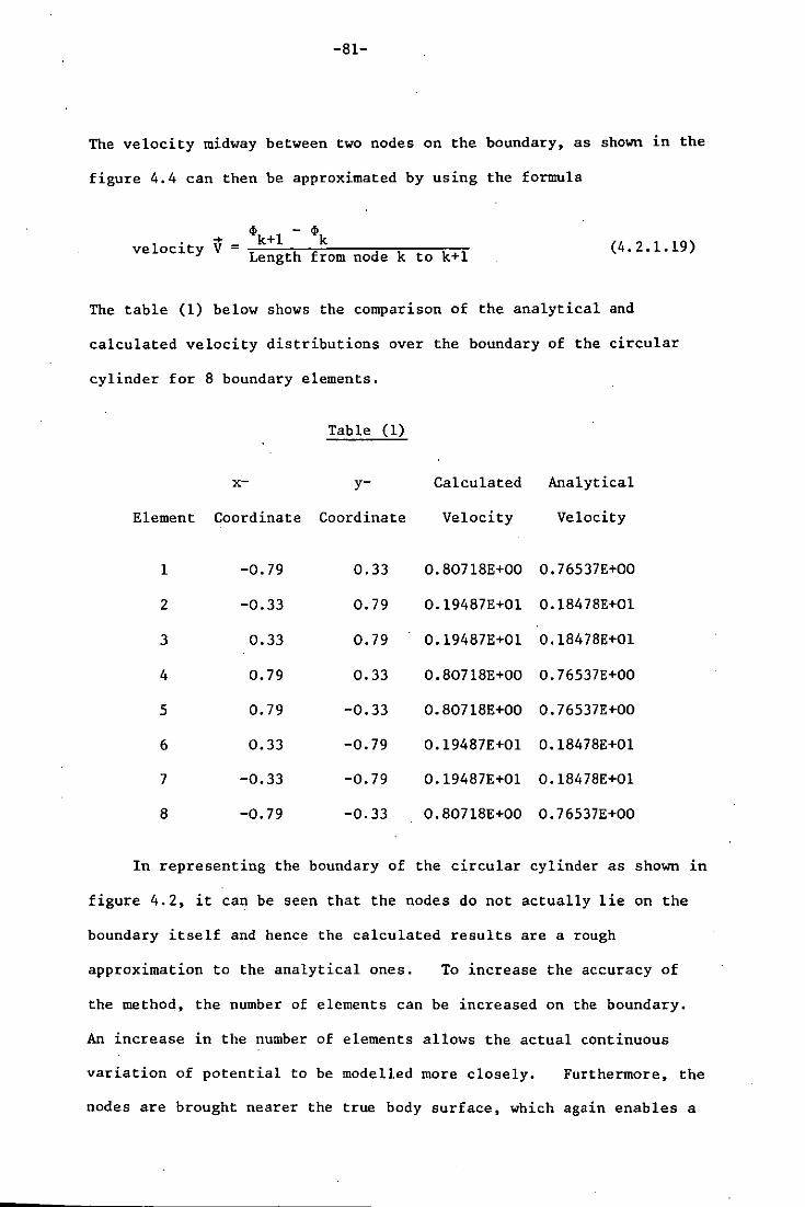
-81-

The velocity midway between two nodes on the boundary, as shown in the

figure 4.4 can then be approximated by using the formula

velocity V Length from node k to k+l (4.2.1.19)

The table (1) below shows the comparison of the analytical and

calculated velocity distributions over the boundary of the circular

cylinder for 8 boundary elements.

Table (1)

x- y- Calculated Analytical

Element Coordinate Coordinate Velocity Velocity

1 -0.79 0.33 0.807l8E+00 0.76537E+00

2 -0.33 0.79 0.19487E+Ol 0.18478E+Ol

3 0.33 0.79 0.l9487E+Ol 0.l8478E+Ol

4 0.79 0.33 0.80718E+00 0.76537E+00

5 0.79 -0.33 0.80718E+00 0.76537E+00

6 0.33 -0.79 0.l9487E+Ol 0.l8478E+Ol

7 -0.33 -0.79 0.l9487E+Ol 0.l8478E+Ol

8 -0.79 -0.33 0.80718E+00 0.76537E+00

In representing the boundary of the circular cylinder as shown in

figure 4.2, it can be seen that the nodes do not actually lie on the

boundary itself and hence the calculated results are a rough

approximation to the analytical ones. To increase the accuracy of

the method, the number of elements can be increased on the boundary.

An increase in the number of elements allows the actual continuous

variation of potential to be modelled more closely. Furthermore, the

nodes are brought nearer the true body surface, which again enables a

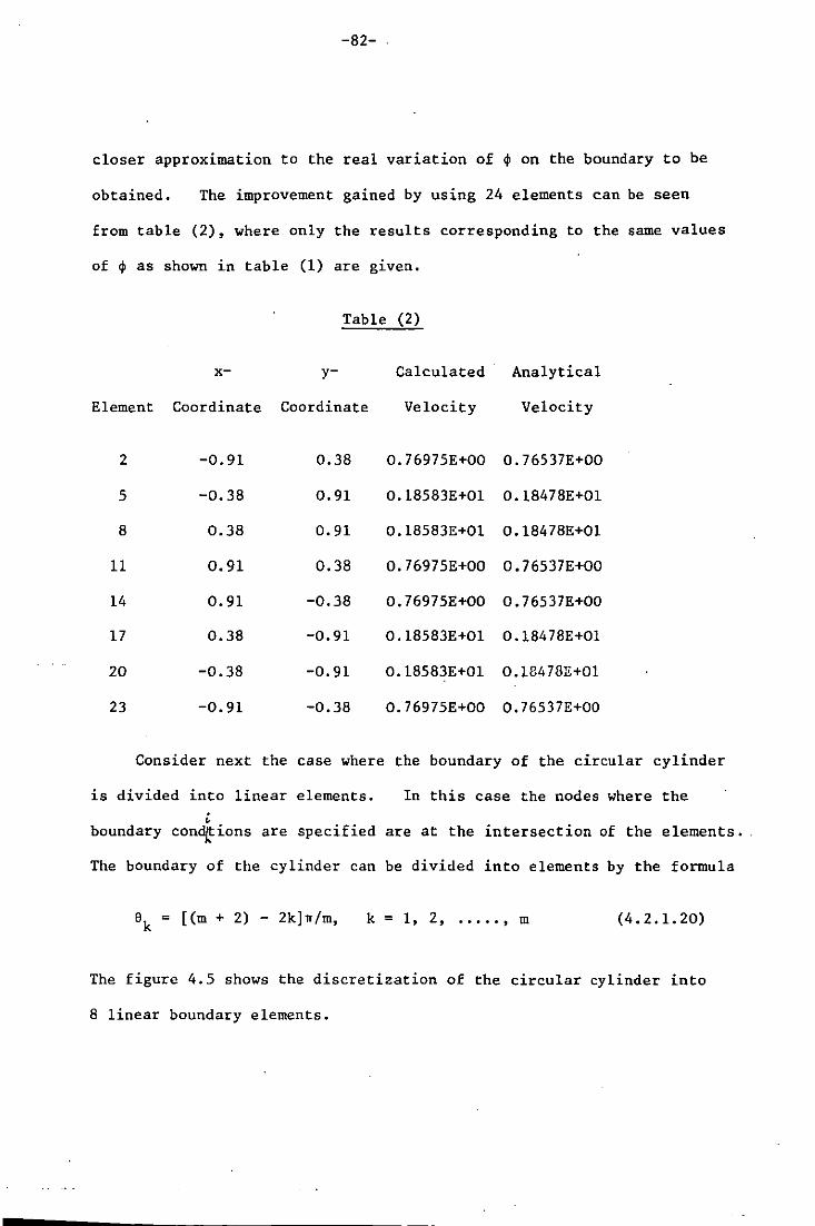
-82-

closer approximation to the real variation of ~ on the boundary to be

obtained. The improvement gained by using 24 elements can be seen

from table (2), where only the results corresponding to the same values

of ~ as shown in table (1) are given.

Table (2)

x- y- Calculated Analytical

Element Coordinate Coordinate Velocity Velocity

2 -0.91 0.38 0.76975E+00 0.76537E+00

5 -0.38 0.91 0.18583E+Ol 0.18478E+Ol

8 0.38 0.91 0.18583E+Ol 0.18478E+Ol

11 0.91 0.38 0.76975E+00 0.76537E+00

14 0.91 -0.38 0.76975E+00 0.76537E+00

17 0.38 -0.91 0.18583E+Ol 0.18478E+Ol

20 -0.38 -0.91 o. 18583E+Ol 0.1847311+01

23 -0.91 -0.38 0.76975E+00 0.76537E+00

Consider next the case where the boundary of the circular cylinder

is divided into linear elements. In this case the nodes where the

• boundary con~ions are specified are at the intersection of the elements •.

The boundary of the cylinder can be divided into elements by the formula

8k = [(m + 2) - 2k]w/m, k = 1, 2, ..... , m (4.2.1.20)

The figure 4.5 shows the discretization of the circular cylinder into

8 linear boundary elements.

-83-

fi xed Poi nt

~i x

Figure 4.5

The coordinates of the extreme points of the elements and the

coordinates of the mid-point of each element where the velocity will

be calculated can be found from the equations (4.2.1.11) and (4.2.1.12)

respectively. The reason for distributing the elements in this way is

such that the velocities are calculated at the same values of e in both

figures 4.4 and 4.5, so that the calculated results could be easily

compared.

The boundary condition (4.2.1.9) in this case takes the form

arp c. c Ux =

an

= x taking U = 1

Equation (2.3.4) can be written for this case as

-c. rp. + 1 1

m 1:

j=l

(4.2.1.21)

J ~(...!.. log 2:) df an LZ1T r

fj (4.2.1.22)

-84-

a41 . Since 41 and an vary linearly over the element, their values at any point

on the element can be defined in terms of their nodal values and the

shape functions NI and N2 as

.£t - [NI an -

1 :: )

(4.2.1.23)

The integrals along an element 'j' on the L.H.S. of e~uation

(4.2.1.22) can now be written as

f 41 a~ [2~ log t) dr r.-i

J

= f . [NI

r.-1 J

= [h~. 1J

a ( 1 1) N2j- - log - dr an 211 r

h~.j 1 <PI ) 1J 412

where k h ..

1J = f . a ( 1 1) Nk an 211 log r dr, k = 1, 2.

r.-1 J

(4.2.1.24)

The integrals on the R.H.S. of equation (4.2.1.22) can be written as

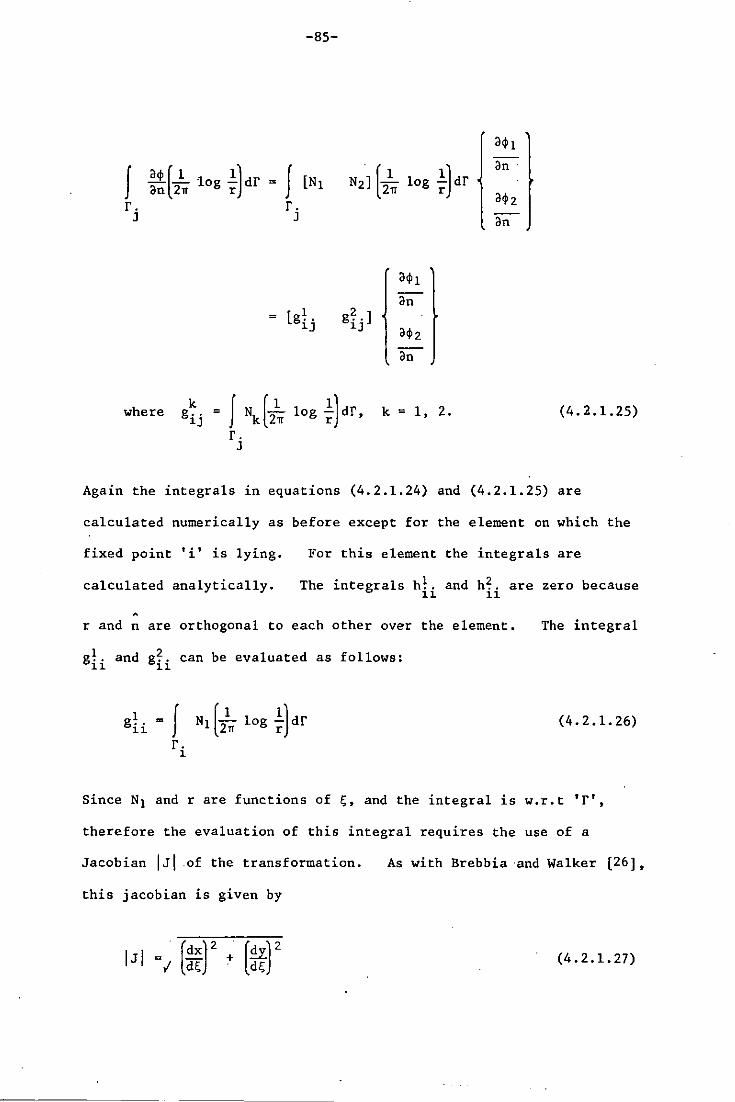
f acp ( 1 1) - - log - df ~ an 211 r f.

J

-85-

f [NI f.

J

[gL 1J

N2] [2~ log ~) df

g?] 1J

where g~j ~ f Nk(2~ log ~)df' k ~ 1, 2.

f. J

Again the integrals in equations (4.2.1. 24) and

calculated numerically as before except for the

fixed point tit is lying. For this element the

calculated analytically. The integrals h!. and 11

a<h

an

ah

an

(4.2.1.25)

(4.2.1.25) are

element on which the

integrals are

h? are zero because n

rand n are orthogonal to each other over the element. The integral

g!. and g? can be evaluated as follows: 11 11

(4.2.1.26)

Since NI and r are functions of ~, and the integral is w.r.t 'f',

therefore the evaluation of this integral requires the use of a

Jacobian I J I .of the transformation. As with Brebbia ·and Walker [26],

this jacobian is given by

(4.2.1.27)

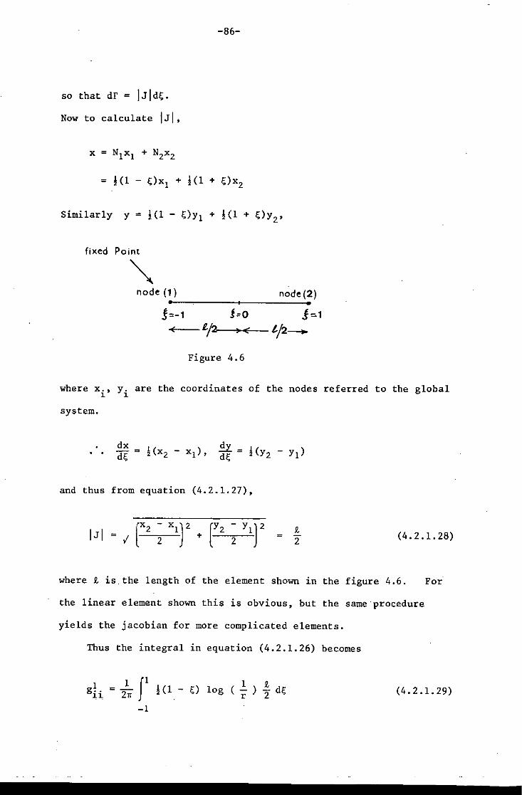
-86-

so that dr = IJld~.

Now to calculate IJI,

Similarly y = !(l - ~)Y1 + !(l + ~)Y2'

fixed Point

node (1) node(2) • •

5=-1 1:0 -<i('-- 1./2 • <

Figure 4.6

where x., y. are the coordinates of the nodes referred to the global 1 1

system.

and thus from equation (4.2.1.27),

R,

2 (4.2.1.28)

where R, is. the length of the element shown in the figure 4.6. For

the linear element shown this is obvious, but the same·procedure

yields the jacobian for more complicated elements.

Thus the integral in equation (4.2.1.26) becomes

1(1 - ~) log ( ! ) ! d~ . r 2 (4.2.1.29)

-1

-87-

If node (1) is taken as the fixed point ••• ~ , then r is measured from

node (1), therefore

r=&'(1+!;) 2

From equations (4.2.1.29) and (4.2.1.30),

= ..!- J1 8n

1 (1 - !;) 10 g 79. --=--- d!;

"2 (1 + !;) -1

9. . = - Lt

8n £-+0+ J1 1

(1 - !;) log -~-- d!;

-1+£ 9. (1 + !;) 2

Integrating by parts and simplifying, then

Similarly, 2 g .. ~~

1 J1 = - !(1 2n + !;) log ~ IJI d!;

-1

(4.2.1.30)

(4.2.1.31)

(4.2.1.32)

Using equations (4.2.1.28) and (4.2.1.30), equation (4.2.1.32) takes

the form

2 =..!- J1 gii 8n 1 (1 + !;) log "'9.--=---- d!;

"2 (1 + !;) -1

=..!- Lt f1 (1 8rr £-+0+

-1+£

1 + !;) log "'9.--=---- d!;

"2 (1 + !;)

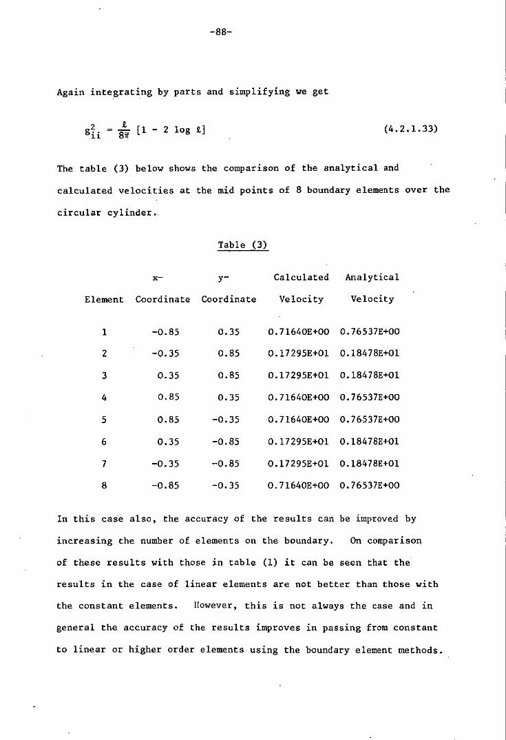
-88-

Again integrating by parts and simplifying we get

(4.2.1.33)

The table (3) below shows the comparison of the analytical and

calculated velocities at the mid points of 8 boundary elements over the

circular cylinder.

Table (3)

x- y- Calculated Analytical

Element Coordinate Coordinate Velocity Velocity

1 -0.85 0.35 0.71640E+00 0.76537E+00

2 -0.35 0.85 0.17295E+Ol 0.18478E+Ol

3 0.35 0.85 0.17295E+Ol 0.18478E+Ol

4 0.85 0.35 0.71640E+00 0.76537E+00

5 0.85 -0.35 0.71640E+00 0.76537E+00

6 0.35 -0.85 0.17295E+Ol 0.18478E+Ol

7 -0.35 -0.85 0.17295E+Ol 0.18478E+Ol

8 -0.85 -0.35 0.71640E+00 0.76537E+00

In this case also, the accuracy of the results can be improved by

increasing the number of elements on the boundary. On comparison

of these results with those in table (1) it can be seen that the

results in the case of linear elements are not better than those with

the constant elements. However, this is not always the case and in

general the accuracy of the results improves in passing from constant

to linear or higher order elements using the boundary element methods.

-89-

4.2.2 FLOW PAST A SPHERE

The body shape that received the greatest attention is naturally

the sphere because it is one of the simplest three-dimensional

symmetrical bodies and has an analytical solution with which the

calculated solutions can be compared. Let the sphere be of radius 'a'

with centre at the origin and let the onset flow be the uniform

stream of velocity U in the positive direction of the x-axis as shown

in the figure 4.7.

y

)

u--~> x

> )

Figure 4.7

The pressure distributions over the surface of the sphere can be

calculated analytically, Vallentine [32], and is given by the formula

C = 1 - ± sin2e p 9 (4.2.2.l)

The boundary condition to be satisfied over the surface of the

sphere can be obtained in a similar manner as for the case of the

-90-

circular cylinder and takes the form

aCPsphere an U -;:;;~x:;:::;:::::;;:

'x2 + y2 + z2

The equation of the surface of the sphere is

where the radius a is taken as 1.

Therefore equation (4.2.2.2) becomes

aCP sphere = an Ux

= x, taking U = 1

(4.2.2.2)

(4.2.2.3)

(4.2.2.4)

The f1owfie1d around the sphere is calculated using different

numbers of boundary elements to approximate the body surface. The

method of element distribution which has been applied is as follows:

z

y

Figure 4.8

Consider the surface of the sphere in one octant to be divided into

three quadrilateral elements by joining the centroid of the surface

with the mid points of the curves in the coordinate planes as shown in

-91-

the figure 4.8. Then each element is divided further into four elements

by joining the centroid of the surface with the mid point of each side

of the element. Thus one octant of the surface of the sphere is divided

into 12 elements and the whole surface of the body is divided into 96

boundary elements. One can then continue to divide each element into

four separate elements by the method mentioned above such that the total

surface of the sphere would be divided in 384 boundary elements, and so

on. The above mentioned method is adopted in order to produce a uniform

distribution of elements over the surface of the body. Figures 4.16

and 4.17 show the discretization of the sphere into 96 and 384 boundary

elements respectively.

As the body possesses planes of symmetry, this fact may be used in

the input to the program and only the non-redundant portion need be

specified by input points. The other portions are automatically

takeri into account. The planes of symmetry are taken to be the

coordinate planes of the reference coordinate system. The advantage

of the use of symmetry is that it reduces the order· of the resulting

system of equations and consequently reduces the computing time in

running a program. As a sphere is symmetric with respect to all the

three coordinate planes of the reference coordinate system, only one

eighth of the body surface need be specified by the input points,

while the other seven-eiehths can be accounted for by symmetry.

However, since the boundary element methods are to be applied to road

vehicles which are symmetric with respect to only one plane, it was

decided to make use of only this one plane of symmetry for all the

bodies considered, namely the xy-plane. Where the body intersects its

plane of symmetry, the points in this plane, (i.e. the points having

z = 0) must be included among the input points.

After the integrals of the equation (2.3.3) for the direct

-92-

boundary element method have been calculated numerically over each of

the boundary elements, the equation (2.3.3) can be put in the matrix

form (3.3.21).

In order to evaluate the potential at each node on the surface it

is necessary to d$ .

'f sphere speC1 y dn at each node, given by (4.2.2.4).

The total velocity potential of the flow, ~, can then be obtained in a

similar way to that for the circular cylinder [equation (4.2.1.4)],

and can then be used to calculate the velocity. The velocity at any

point on an element can then be found as follows:

The x, y and z components of the velocity are given by

[d<l> dX '

d<l» • 1 az respect1ve y. Now

and

Furthermore as there must be zero normal velocity on the surface of the

body, then

n.\7~ = 0

or (4.2.2.5)

The complete system of the equations can be written in matrix form as

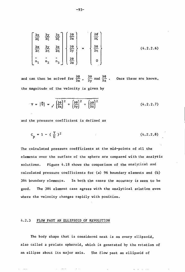
-93-

ax ~ az a4> ar; ar; ar; ax

ax ~ 3z a4> =

a" a" a" ay

a4> n 1 n2 n3 az

34> and can then be solved for ax '

af 3r;

a4> a"

0

~and ~ ay 3z

the magnitude of the velocity is given by

and the pressure coefficient is defined as

C = 1 - ( ~ )2 P U

(4.2.2.6)

Once these are known,

(4.2.2.7)

(4.2.2.8)

The calculated pressure coefficients at the mid-points of all the

elements over the surface of the sphere are compared with the analytic

solutions. Figure 4.18 shows the comparison of the analytical and

calculated pressure coefficients for (a) 96 boundary elements and (b)

384 boundary elements. In both the cases the accuracy is seen to be

good. The 384 element case agrees with the analytical solution even

where the velocity changes rapidly with position.

4.2.3 FLOW PAST AN ELLIPSOID OF REVOLUTION

The body shape that is considered next is an ovary ellipsoid,

also called a prolate spheroid, which is generated by the rotation of

an ellipse about its major axis. The flow past an ellipsoid of

-94-

revolution is an axisymmetric flow and has some analogies with the two­

dimensional flow; in particular, a stream function ~ can be defined,

and, of course, when the motion is irrotational, a velocity potential

always exists.

The accuracy of the computed results is best checked by comparing

them with analytical results. The stream function for flow past an

ovary ellipsoid is given in Milne-Thomson [24) and the velocity distribution

about the ellipsoid can be determined from this, as shown below.

Let an ovary ellipsoid be generated by revolving an ellipse of

semi-major axis a and semi minor axis b. about the x-axis and let the

uniform stream of velocity U be in the positive direction of x-axis as

shown in the figure 4.9.

b

o

Figure 4.9

An axisymmetric flow is most conveniently formulated in cylindrical polar

coordinates. Following Milne-Thomson [24), the cylindrical polar

coordinates are taken as (x, w, w).

x

-95-

In Milne-Thomson [241. the ovary ellipsoid is. defined by the

transformation

x + iw = c cosh ~

= c cosh (I; + in)

= c cosh I; cos n + ic sinh I; sin n

Comparison of real and imaginary parts gives

x c cosh I; cos n

w = c sinh I; sin n (4.2.3.1)

and therefore the curve I; = 1;0 is an ellipse in the xW-plane whose

semi-axes are

a = c cosh I; 0

b = c sinh 1;0

and so I; = 1;0 is an ovary ellipsoid.

(4.2.3.2)

The stream function W for an ovary ellipsoid moving in the

negative direction of the x-axis with velocity U is given in Milne-

Thomson [241. art 16.57 as

~2(COSh I; + sinh2 I; log tanh t ) w = -=---------------'=--

a b 2 a + b - c c + C2 log a + b + C

(4.2.3.3)

Also. the stream function W for the uniform stream with velocity U. in

the positive direction of x-axis is given in Milne-Thomson [241. art

16.22 as

w = -jUw2 (4.2.3.4)

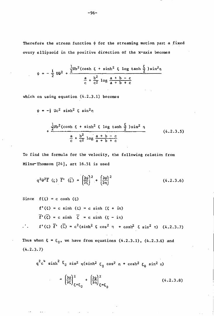
-96-

Therefore the stream function 1jI for the streaming motion past a fixed

ovary ellipsoid in the positive direction of the x-axis becomes

~2(COSh , + sinh2 , log tanh t )sin2n 1jI=-.!.Uw2 +

2 a b 2 a + b - c C + C2 log a + b + c

which on using equation (4.2.3.1) becomes

~2(COSh , + sinh2 , log tanh t )sin2 n + ~------------------------~~------

a b 2 . a + b - c C + C2 log a + b + C

(4.2.3.5)

To find the formula for the velocity, the following relation from

Mi1ne-Thomson [24], art 16.51 is used

since f(~) = c cosh (~)

f'(~) = c sinh (~) = c sinh (~ + in)

i'(~) = c sinh ~ = c sinh (~ - in)

(4.2.3.6)

f' (~) i' (~) = c2(sinh2 , cos 2 n + cosil , sin2 n) (4.2.3.7)

Thus when' = '0' we have from equations (4.2.3.1), (4.2.3.6) and

(4.2.3.7)

(4.2.3.8)

-97-

Now from equation (4.2.3.5)

[awl = -uc2 sinh ~o cosh ~O sin2 11 a~ /;;=/;;

o

Ub 2[sinh /;;0 + sinh /;;0 cosh /;;0 tanh ~ lsin2 11 + --------~--------------~----~~------

a b 2 a + b - c - + -,.- log ~.,.....;c:......,~ C c< a + b + C

which on using equation (4.2.3.2) takes the form

[b3

a b ~ 1] c + bee log tanh Sf a hI a+b-c - + l:- og --.,....,f-.,---~ c c a+b+c

Let us find tanh ~ in terms of a, band c.

From equation (4.2.3.2),

c cosh /;;0 ' - = b a

- = c sinh ~O

c 2 sinh ~ cosh fQ

2 2 or ~ = 2 cosh2 Sf - 1, - = b

sinh ~ tanh II = ___ -:'2"--

2 cosh !'.f =

2 sinh!'.f cosh !ft 2 cosh2 In.

2

(4.2.3.9)

= b/c a + 1 c

b = ---''-­a + c (4.2.3.10)

Now a + b - c a + b + c

since a2

b a 2 - b 2 - c 2

a + c = (a + b + c)(a + c) = 0

. . a + b - c a + b + C

b = --:­a + c

-98-

From equation (4.2.3.10) and (4.2.3.11),

tanh ~ = a + b - c 2 a+b+c

Equation (4.2.3.9) takes the form

= U sinz

n [~

Also from equation (4.2.3.5),

-c- + -c- 10 g "a--:+--7b--:+--"-c b3

ab3

a + b - c] + ~a--~b~Z------a~+--b~---c~

C + -c-z log a + b + C

:-cb bZ a + b -

+ Cl log a + b + ~]

(4.2.3.11)

(4.2.3.12)

(4.2.3.13)

F; Ub z [cosh F;o + sinhZF;o log tanh T 1 sin n cos n

+ --------------~O-~--~~--=------------a b Z a + b - c - + ....,.. log C cL. . a + b + C

and from equations (4.2.3.2) and (4.2.3.12), this becomes

[!tl - " .i. " 000 "[ ob' •

Z r a bZ

a + b - cl] b .c + clog a + b +

an F;=F;o a b a + b - c - +-- log c c a + b + C

0 (4.2.3.14)

as clearly should be the case.

Using equations (4.2.3.13) and (4.2.3.14), equation (4.2.3.8) becomes

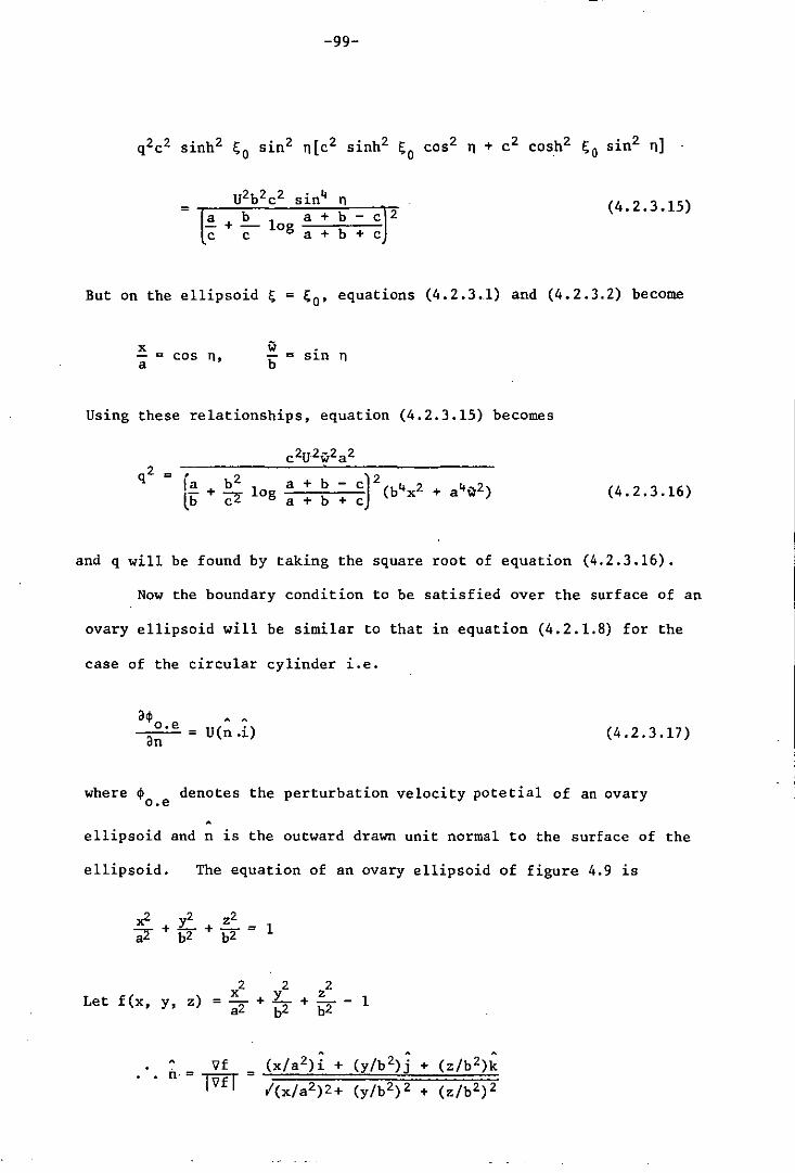
-99-

(4.2.3.15)

But On the ellipsoid /; = /;0' equations (4.2.3.1) and (4.2.3.2) become

~ = cos n, a ~ = sin T1

Using these relationships, equation (4.2.3.15) becomes

fa b2 a + b - c)2(b4x2 l-b +"""'c log r~ a + b + C

(4.2.3.16)

and q will be found by taking the square root of equation (4.2.3.16).

Now the boundary condition to be satisfied OVer the surface of an

ovary ellipsoid will be similar to that in equation (4.2.1.8) for the

case of the circular cylinder i.e.

. . = U(n .i) (4.2.3.17)

where $ denotes the perturbation velocity potetial of an ovary o.e

ellipsoid and n is the outward drawn unit normal to the surface of the

ellipsoid. The equation of an ovary ellipsoid of figure 4.9 is

Xl • .2 z2 --,r+L-+-=1 a~ b2 b2

Let f(x, y, z)

, 'If n· = TVfT

-100-

Therefore the boundary condition in equation (4.2.3.17) takes the form

(4.2.3.18) Ib4x2 + a4(y2 + z2)

The calculated velocity distributions are compared with analytical

solutions for the ellipsoids of fineness ratios 2 and 10. In both

cases of ellipsoi~of revolution" the input points are distributed on

a sphere in the manner described in the section (4.2.2), and the y and

z coordinates of these points are then divided by the fineness ratios

to generate the points for the ovary ellipsoids. This procedure is

easy and t~nds to concentrate the points .in the regions of high

curvature of the body surface, but the uniformity of the element

distribution becomes poor. The number of elements used to obtain the

calculated velocity distribution are the same as were used for the

sphere. Figures 4.19 and 4.20 show the discritization of the ovary

ellipsoid of fineness ratio 2 into 96 and 384 boundary elements

respectively. Figure 4.21 shows the comparison of the analytical and

calculated velocity distributions over the surface of an ovary

ellipsoid of fineness ratio 2 for (a) 96 boundary elements and (b) 384

boundary elements.

Similarly figures 4.22 and 4.23 show the discretization of the

ovary ellipsoid of fineness ratio 10 into 96 and 384 boundary elements

respectively. Figure 4.24 shows the comparison of the analytical and

calculated velocity distributions over the surface of an ovary ellipsoid

of fineness ratio 10 for (a) 96 boundary elements and (b) 384 boundary

elements. The accuracy of the calculated results in both cases of

-101-

ellipsoids of fineness ratio 2 and 10 is .seen to be quite good. The

384 element case in both ovary ellipsoids agree with the analytical

solutions even in the region. near the stagnation point where the

velocity varies rapidly with position.

4.3 EFFECTS OF A GROUND PLANE

Thus far the body under consideration has always been assumed to

be positioned in an infinite space. The flow field around any body

lying in a free atmosphere is different from the flow field around the

same body at the same attitude when it is lying very.close to the

ground. Therefore simulation of the ground flow is an important

feature to be incorporated in the theory. The inviscid flow over

the ground, which is considered to be a plane, remains everywhere

tangential to its surface. This flow is simulated by the so-called

'mirror image' principle. A mirror image of the body is imagined to

be present below the ground plane. The flow field produced by a unif­

orm stream, parallel to the gvound plane, which is perturbed by the

body and its image is then symmetrical with respect to the ground

plane. The plane of symmetry is a stream surface and represents the

ground, see figure 4.10.

-102-

y

x

BODY

n>>>;;;"" ;;,;;;;,.,.}; Hr >nnn", nn In;, In nn;, ;;;,; ;;;;; ; ;,;7,;; j" »;",,;;;;;,;;.

IMAGE BODY

GROUND PLANE

x o»---------~~--------~----~

y

Figure 4.10

Figure 4.11 illustrates how the influences of the image body on

the real body are calculated.

-103-

y x

z

//11/ 77!71!JlJ 7/l7l77 1/777 77/71777 /111/1 7!lJJ 771/ 7/ /7/ /77 1/77/7 7 /771f GROUN PLANE

@] 0 0', z , , , , , , , ,

x y

Figure 4.11

Suppose side (1) is the side at which the values of the potential

are to be evaluated at the fixed points , . , ~ . At a given point, the

components of the H .. and G.. integrals due to an element on side (1) 1J ~J

are evaluated first. The z-coordinates of all the nodes of this

element are then changed (side (2» and the components from this

reflected element are calculated. The y-coordinates of all the nodes

of this element are then changed (side (3» and the components from

this element are evaluated. Position (4) is then reached by

changing the z coordinates again and evaluating the components due to .

the e lemen t. The integral componets from the corresponding elements

-104-

on all the four sides are then summed to calculate the total integral

values at the point on side (1) due to one particular element on side

(1). The process is repeated for all the elements on side (1) and

then for all the fixed points. The pressure distribution over the

surface of a sphere of radius 1 unit with ground clearance of 0.1 units

and 0.3 units has been calculated using the above method. The pressure

coefficient over the surface of the sphere is calculated for 96, 384

and 1536 boundary elements. To check the accuracy of the calculated

results, these have been compared with the analytical results given in

Peat [33]. Figures 4.25 and 4.26 show the comparisons of the

calculated and analytical pressure coefficients over the surface of the

sphere for (a) 96 and (b) 384 boundary elements, with ground clearances

of 0.1 units and 0.3 units respectively. The analytical solutions are

based upon a truncated series of images of doublets and line doublets.

The truncation causes no serious error for a ground clearance of 0.3

units, but in the case of 0.1 units the results near the ground may be

inaccurate in the first decimal place. .For this reason, the pressure

distribution over the surface of the sphere was also obtained for 1536

boundary elements, to hopefully give a more accurate standard for

comparision of the low element cases than is possible from the

analytical solution near the ground. Figure (4.27) shows the

discretization of the sphere into 1536 boundary elements, whilst figure

(4.28) shows the comparison of the analytical and computed pressure

coefficients with the ground clearances of 0.1 and 0.3 units. From

these figures one can deduce that the basic modelling of the ground

plane for the boundary element method is correct.

-105-

4.4 MODELLING OF A WAKE

Thus for in the ·ana1ysis of the flow field, the viscosity of the

fluid has been neglected. However, all fluids are viscous to some

extent, and thus in problems of aerodynamics, there is a region of the

flow field near the body where the viscosity plays an important role.

If the body under consideration is streamlined, then the boundary layer

will cover the body from front to the rear end, producing a wake of

negligible thickness. On the other hand, in vehicle aerodynamics, the

road vehicle is a bluff body and thus the boundary layer separates from

the body producing a thick wake.

Let the body under consideration be as shown in the figure 4.12.

Domain R

Figure 4.12

In this case, the surface of the body is S = SB + ~, where SB denotes

the surface of the actual body and ~ the surface of the tubular wake

which starts from the back of the body and extends to infinity in the

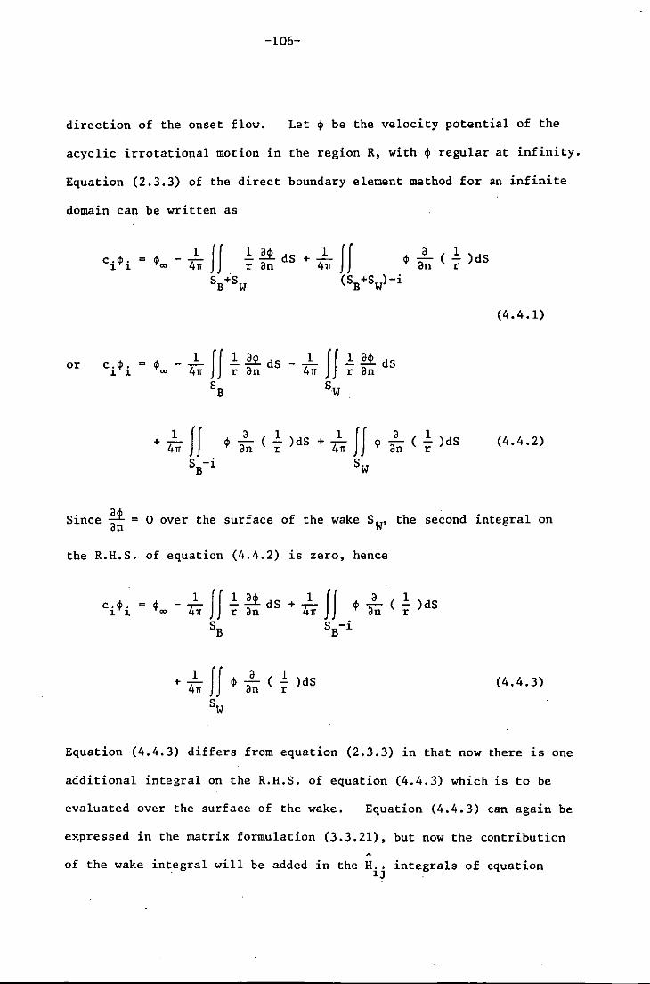
-106-

direction of the onset flow. Let $ be the velocity potential of the

acyclic irrotational motion in the region R, with $ regular at infinity.

Equation (2.3.3) of the direct boundary element method for an infinite

domain can be written as

(4.4.1)

or ci$i = $w - 4111 Jf ~ *" dS

SB

- ...!.. II 1:. 2.t dS 411 r an

$ a ( 1 )dS an r

Sw

a (1:.) dS an r

(4.4.2)

. ~ o over the surface of the wake SW' the second integral on S~nce = an

the R.H.S. of

c.$. $w = ~ ~

equation (4.4.2) is zero,

- ...!.. JJ 1:. ~ dS 411 r an + 41

11 JJ SB S -i B

$ a ( 1 )dS an r

hence

$ a ( 1:. )dS an r

(4.4.3)

Equation (4.4.3) differs from equation (2.3.3) in that now there is one

additional integral on the R.H.S. of equation (4.4.3) which is to be

evaluated over the surface of the wake. Equation (4.4.3) can again be

expressed in the matrix formulation (3.3.21), but now the contribution

of the wake integral will be added in the H .. integrals of equation ~J

-107-

(3.3.20) • The matrix system can again be solved for unknown velocity

potentials and thus the pressure coefficients over the surface of the

body can be calculated by the same method outlined in the preceding

sections.

The integral over the surface of the wake can be evaluated as

follows:

Denoting this integral by I, then

I 1 fJ <P

a (

1 )dS =-411 an r

Sw

1 It a 1 (4.4.4) =- <P ( - )dxdr 411 an r r -00

where Xo is the starting point of the wake and r is the closed curve

bounding the tubular wake at its point of origin.

Since the wake is assumed to be tubular (i.e. parallel to the

x-axis), then on the surface of the wake the velocity is the free-

stream velocity, that is

ax

~ = 0, over the surface of the wake, where <p is the perturbation

velocity potential.

Thus <p is constant over the wake, or, as the wake is semi-infinite it

is possible for <p to have a finite linear variation with respect to 'x'

over the complete wake strip. In the first instance, consider that <p

is constant, then equation (4.4.4) can be written as

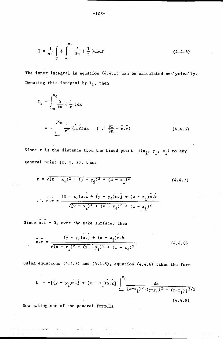
I = 41" J

r

-108-

a (1. )dxdr an r (4.4.5)

The inner integral in equation (4.4.5) can be calculated analytically.

Denoting this integral by 11 , then

1 ( - )dx r

(0 ~ (n.r)dx (" •• _ar = an n.r) (4.4.6)

since r is the distance from the fixed point i(xi

, Yi' zi) to any

general point (x, y, z), then

r = i(x - x.)2 + (y - y.)Z + (z - z.)Z 1 1 1

.. (x - x.)n.i + (y - y.)n.j + (z - z.)n.k 111

n. r = -17====~=7=;==~;:::::::;:===~­i(x - x.)z + (y - y.)z + (z _ z.)z . 1 1 1

Since n.i = 0, over the wake surface, then

(y - y.)n.j + (z - z.)n.k 1 1

n • r = --;T====::;;:=:;===:::::;::;:::~====::::;;:­i(x - x.)2 + (y y.)Z ~ (z _ z.)Z 111

(4.4.7)

(4.4.8)

Using equations (4.4.7) and (4.4.8), equation (4.4.6) takes the form

I = -[(y - y.)n.j + (z - z.)n.k] 1 1

(4.4.9) Now making use of the general formula

-109-

J dx = --::-:;---;--2=-(~2:::a~x=+;::b=):;::~= (ax2 + bx + c) 3/2 (b2 - 4ac) ,tax2 + bx .+ c

the integral in equation (4.4.9) can be evaluated as follows:

dx [x2 _ 2x.x + x~ + (Y - y.)2 + (z _ z.)2]3/2

1. 1. 1. 1.

(x - x.) 1.

(z-z.)2] [x2 - 2x.x + x~ .. + (y_y.)2 1. 1. 1. 1.

1 =------'=-----[(y_y.)2 + (z-z.)2]

1. 1.

I (x o - xi) l ~-[ (-X-o---x-

i-)2-+-(-y-=--y-i)-2-"-+-(-Z--z-1.-. )-2-]Tj + J

From equation (4.4.9) and (4.4.10)

[(y-y.)n.j + (z-z.)n.k] [ 1. 1. 11 = - ---=------=---

[(y_y.)2 + (z-z.)2] 1. 1.

(Xo + xi)

(y_y.)2 + 1.

Substituting this value of 11 in equation (4.4.5), then·

(4.4.10)

(4.4.11)

1=-...!..J4> (Y-Yi)n. J + (Z-Z.)~.kr (xo - xi) ,l

-[-(Y-'-=-Y-i-) -2 -+-(-Z--z-':=-)-2-] -I~-[ (-X-O---X-i-) 2-+-(":Y---Y-i)-'2=-+-(-Z---Z-i)-2-]-;-! + lJ dr 4n

r

(4.4.12)

Suppose that the closed curve r is divided into m1 two dimensional

boundary elements. m1 is also the number of boundary elements on the

-110-

surface of the body associated with the wake. The two-dimensional

isoparametric boundary elements can be linear, quadratic or cubic,

corresponding to the variation chosen for the quadrilateral elements

over the surface of the body. Thus ~, over the two-dimensional

boundary elements, can be written as

(4.4.13)

where L is the number of nodes and is equal to two, three or four in

the case of linear quadratic or cubic elements respectively,

~k are the nodal values of ~ and Ilk are the shape functions as defined

in equations (3.2.1) or (3.2.2) or (3.2.3).

Using equation (4.4.13), equation (4.4.12) becomes

1 ml J [NI

(y - y.)n.j + (z z.)n.k I = - - E N2 ••• NL] 1. 1.

411 . 1 [(y _ y.)2 + (z z. )2] J= r. 1 1 J

[ "'. -(XO - Xi) . j d'

$1

$2 x.)2 + (y _ y.)2 + (z - z.)2]!

1 1 1.

where

[w~ . 1J

w? 1J

~1

... " ;".] ~2 1J

$L

(4.4.14)

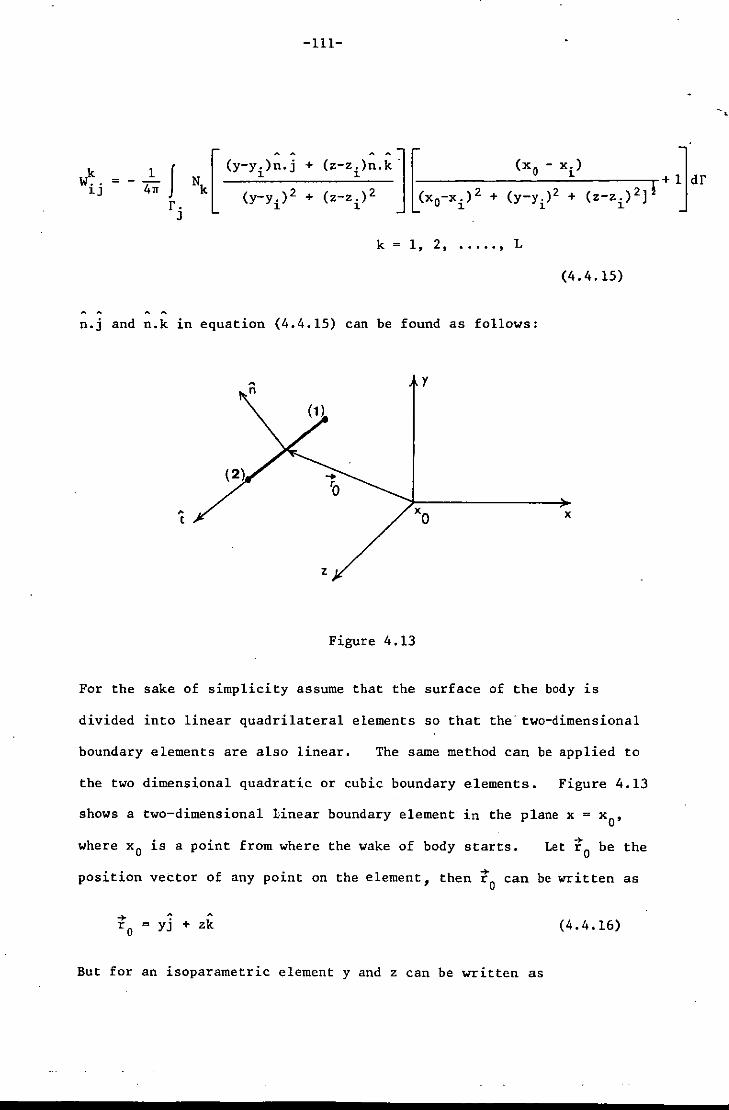
-111-

k = W-.- • 1J

1 J 4rr [

(y-y.)~.j + N 1

k (y_y.)2 + 1 r.

J

k 1, 2, ••.•• , L

(4.4.15)

n.j and n.k in equation (4.4.15) can be found as follows:

~

n y

x

z

Figure 4.13

For the sake of simplicity assume that the surface of the body is

divided into linear quadrilateral elements so that the- two-dimensional

boundary elements are also linear. The same method can be applied to

the two dimensional quadratic or cubic boundary elements. Figure 4.13

shows a two-dimensional Linear boundary element in the plane x = xO'

where Xo is a point from where the wake of body starts. ~ Let robe the

position vector of any point on the element, then to can be written as

A

= yj + zk (4.4.16)

But for an isoparametric element y and z can be written as

-112-

2 2 y = E Nk Yk , Z = E NkZk k=l k=l

or Y !(Y2 - Yl)~ + !(Y2 + Yl)

Z = !(z2 - zl)~ + !(z2 + zl) (4.4.17)

From equations (4.4.16) and (4.4.17),

+ The tangent vector t at any point to the element can be written as

or the unit tangent vector t can be given as

t (Y2 - Yl)j + (z2 - zl)k

I(Y2 - Yl)Z + (z2 - zl)Z

Since the numbering system for the elements on the wake is anti-

clockwise as viewed from the front of the body, then rotating this unit

o tangent clockwise through 90 , the outwardly drawn unit normal n to the

element is given by

, (z2 - zl)j - (Y2 - Yl)k

n = I(Y2 - Yl)Z + (z2 - zl)Z

(4.4.18)

and thus n.j and n.k can be written as

-113-

(zz - zl) n.j =

{(Yz - Yl)2 + (zz _ z )2 1

and

-(yz - Yl) n.k =

I(yz - Yl)Z + (z2 - zl)2 (4.4.19)

With these values of n.j and n.k, the integrals of equation (4.4.15)

can be evaluated numerically using one~dimensional Gauss-quadrature

rule.

Thus f~r, the value of $ in equation (4.4.4) has been taken to be

constant with respect to 'x' over the surface of the wake. If one

considers $ to have a linear variation with respect to 'x', it can be

shown that the value of the integral I remains the same, thus the

results obtained above hold in this case as well.

4.4.1 FLOW PAST A SEMI INFINITE BODY

Before the previous analysis was used to calculate the flow

around a ground vehicle, it was felt advisable to compare it with an

analytical solution so that the accuracy of the method could be

checked. Whilst there is no analytical solution to flow around a

bluff body with a wake, the technique used in the boundary element

method was to model the wake as a physical extension of the body,

giving an effectively semi-infinite solid body, and an analytical

solution can be found for uniform flow past some semi-infinite bodies.

Let the semi-infinite body be as shown in the figure 4.14.

r=sec ~ 2

-114-

o

Figure 4.14

R

•

u x

This semi-infinite body is obtained by considering a source of unit

strength lying at the origin in a uniform stream of velocity 1 in the

negative direction of x-axis. It has been shown in Va11entine [32].

that the surface of this semi-infinite body is

e r = sec 2' (4.4.1.1)

and the pressure distribution over the surface of this semi-infinite

body is calculated analytically from the formula

(4.4.1.2)

The surface of the semi-infinite body is approximated using different

number of boundary elements. The method of distribution of elements

is as follows:

hemisphe re of radius 2

r=sec.! R (-a.2)

2 ~

~

(xl·RI) .0<--

WAKE x

...r,....-

..t.--

(-a.-2)

Figure 4.15

U

-1l5-

Divide the surface of a hemisphere of unit radius into boundary

elements in the manner as described in section (4.2.~). Multiply the

coordinates of the input points by 2 to generate the data for the

hemisphere of radius 2. Stretch the hemisphere of radius 2 in the

negative direction of x-axis in such a way that the surface of the

hemisphere is transformed into the shape of a semi-infinite body and

cut the body by a vertical plane at the point x = -a, where a is any

positive constant. In this way the point (2 , 0) and the plane x = 0

of the hemisphere of radius 2 coincide with the point (1 , 0) and the

plane x = -a respectively of the deformed body. The y and z

coordinates of the deformed body are the same as that of the

hemisphere of radius 2, while the x-coordinate of the deformed body is

calculated as follows:

From the figure 4.15,

and x 2 = sec ~ cos e, ~2 = sec ~ sin e = 2 sin ~

Therefore the stretch = xl - x 2

= 2 cos 4> - sec ~ cos e

or e x2 = xl + sec "2 cos e - 2 cos 4>

where <p = tan-l (~ ) •

To calculate e, it can be seen from the figure 4.15 that RI = 1<2

. . 2 sin '" = 2 . e 'I' S1n "2 and e = 24>

-116-

Next, to approximate the deformed body with the semi-infinite body,

a wake will be added to the surface of the deformed body starting from

the plane x = -a and extending to x = -m in the direction of the

uniform stream.

The boundary condition to be satisfied on the surface of the semi-

infinite body is

a~s.inf = -U(n.i) an

-(n.i) taking U = I (4.4.1.2)

where ~ . fdenotes the perturbation velocity potential of the s.1.n

semi-infinite body and n is the outwardly drawn unit normal at each

node on the surface of the semi-infinite body. The problem of

finding this unit normal is slightly more difficult than in previous

examples. The actual method used, given below, was developed for the

general case of road vehicles where it is impossible to define

analytically a unit normal.

Each node on the surface of the semi-infinite body, except in the

symmetry plane, has a maximum of four boundary elements associated with

it and corresponding to each of these boundary elements, the normal at

this node will, in general, have a different direction. Thus the

normal at the node under consideration is calculated with respect to

each of the associated elements and then the mean of all these normals

is taken as the true normal to the surface at that node. For a node

in the symmetry plane, there are a maximum of two boundary elements

associated with this node and to find the true normal, the elements

corresponding to this node on the opposite side of the symmetry plane

are also taken into account. Thus the mean of all the normals at

-117-

this node corresponding to these elements will be taken as the true

normal to the surface at this node.

Figures 4.29, 4.30 and 4.31 show the discretization of the

semi-infinite body into 48, 192 and 768 boundary elements respectively.

In order to have the.uniform distribution of elements at the back of

the body, it is cut by the plane x = -5, x = -10 and x = -20 for the

case of 48, 192 and 768 boundary elements respectively. The pressure

distribution over the surface of these semi-infinite bodies are

calculated using the direct boundary element method. Figure 4.32

shows the comparison of the analytical and calculated pressure

distributions over the surface of the semi-infinite body for (a)48

boundary elements (b) 192 boundary elements, whilst figure 4.33 shows

the comparison for 768 boundary elements. It. is seen that as the

number of boundary elements is increased, the accuracy in the results

is also increased. In the case of 768 boundary elements, there is an

excellent agreement between the analytical and the calculated results.

4.5 COMPARISON OF GAUSS-ELIMINATION AND GAUSS-SEIDEL METHODS

In section (3.5), the general comparison of Gauss-elimination and

Gauss-Seidel iterative methods for solving the system of linear algebraic

equations was presented. It was concluded that in solving a system of

M linear equations, the Gauss-Seidel method is computationally more

efficient if it converges in fewer than M iterations. In this section

the comparison of these two methods for solving the system of equations

which result from the discretization of the body in the case of three­

dimensional exterior flow problems is presented. The following table

-118-

shows the comparison of computing time for the solution stage of equation

systems of different orders. The actual results presented are for

flows about a sphere and a semi-infinite body, but for flow about any

other bodies, the computing time is not significantly different when

the system size is kept the same.

TABLE

Iterations

System Size Gauss-Elimination Gauss-Seidel Required

57 x 57 0.602 0.448 7

113 x 113 4.636 1.559 8

209 x 209 28.823 4.383 7

417 x 417 - ·20.416 9

801 x 801 - 58.048 7

It can be seen from this table that in all cases the Gauss-Seidel

method is more computationally efficient than the Gauss-elimination

method. The gain in efficiency of the Gauss-Seidel method over the

Gauss-elimination method is seen to increase with increasing system

size. The number of iterations required for the convergence of the

Gauss-Seidel method is very small even for large system size.

Convergence of Gauss-Seidel method has been taken to occur when the

greatest iterative change of any single value of potential is less

than 0.00001.

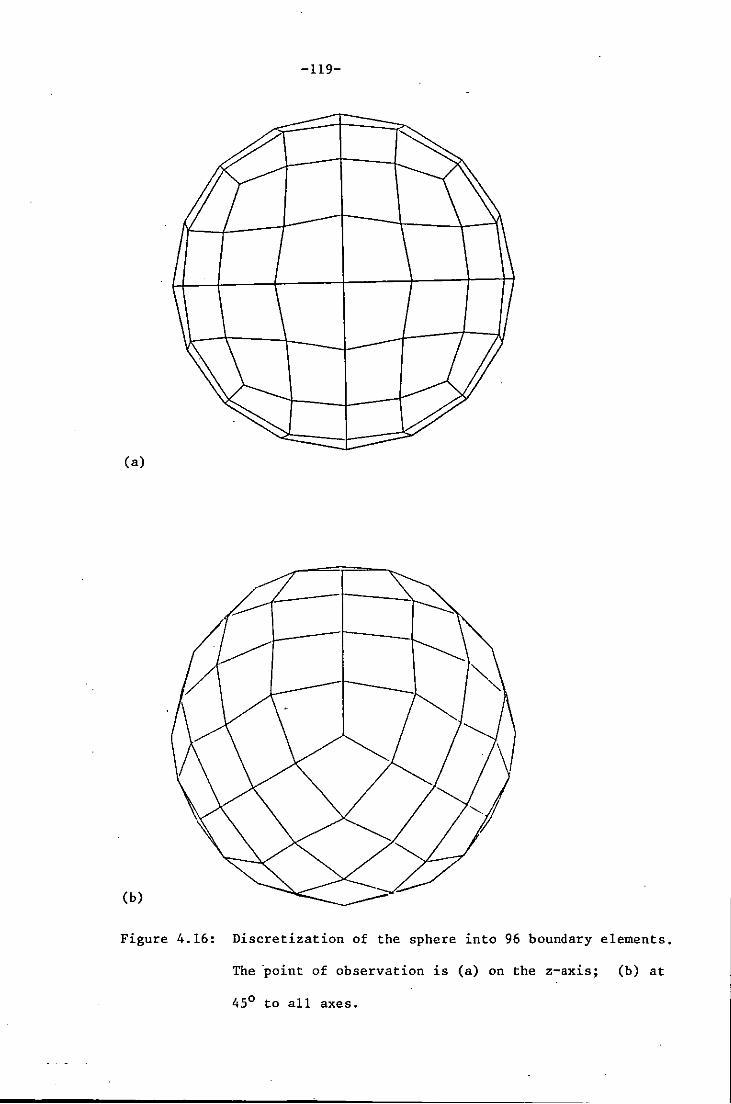
-119-

Ca)

Cb)

Figure 4.16: Discretization of the sphere into 96 boundary elements.

The ·point of observation is Ca) on the z-axis; Cb) at

450 to all axes.

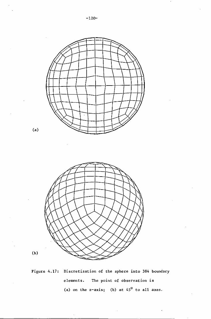
-120-

(a)

(b)

Figure 4.17: Discretization of the sphere into 384 boundary

elements. The point of observation is

(a) on the z-axis; (b) at 450 to all axes.

(a)

(b)

-121-

C 1

C P

p

0~_--~-'-----'--f---T3----~4 e

-1 x

Analytical solution

-2 x Computed solution

01---~~------'-~---3r-----;4 e

-1

-2

Figure 4.18: Comparison of analytical and computed pressure

coefficients on a sphere for (a) 96 boundary elements;

(b) 384 boundary elements.

. .

-122-

(b)

Figure 4.19: Discretization of an ovary ellipsoid of fineness ratio 2

into 96 boundary elements. The point of observation is

(a) on the minor axis; (b) at 450 to all axes.

-123-

(a)

(b)

Figure 4.20: Discretization of an ovary ellipsoid of fineness

ratio 2 into 384 boundary elements. The point of

observation is (a) on the ininor axis; (b) at 450

to all axes.

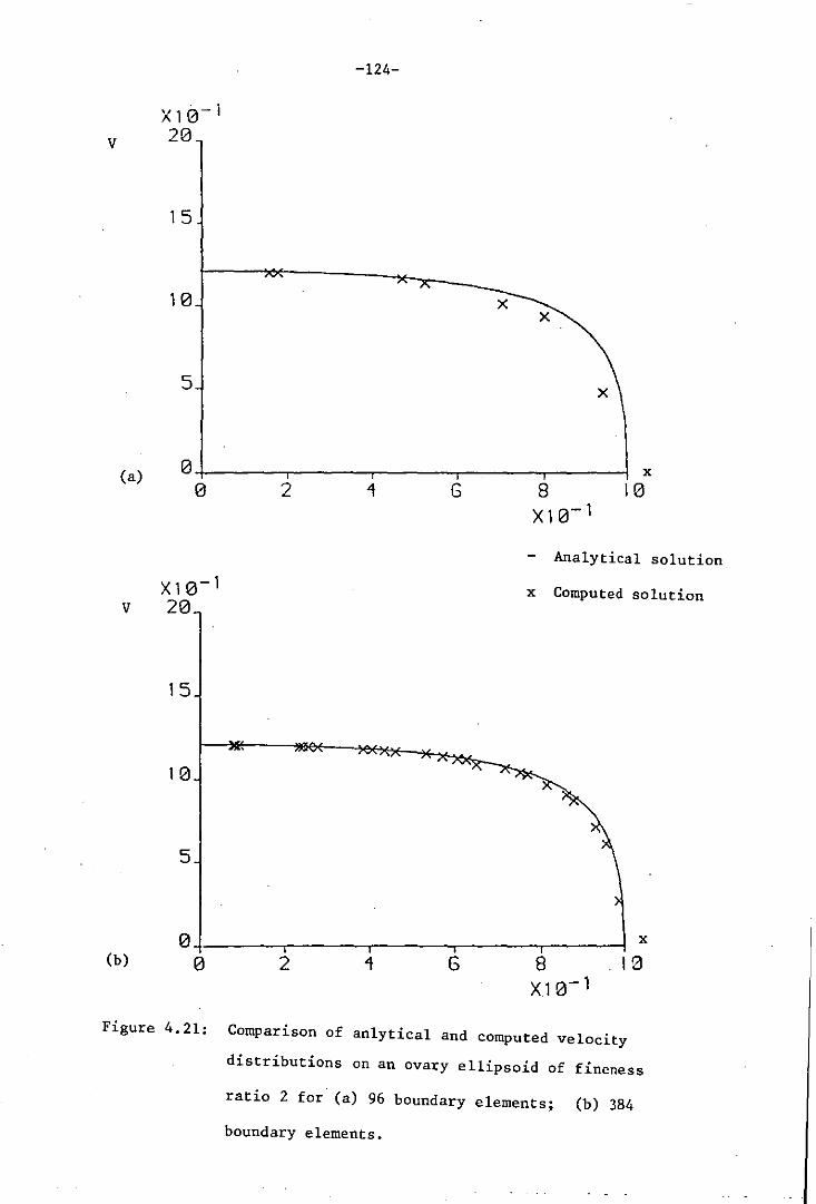
-124-

v

15

10 x x

5 x

(a) 01------r-----.----~------~--~10x o 2 4 G 8

X10- 1

- Analytical solution

x Computed solution v

15

10

5

(b)

x 0j-----r----.-----.-----8~---:13 o 2 G X10- 1

Figure 4.21: Comparison of anlytical and computed velocity

distributions on an ovary ellipsoid of fineness

ratio 2 for (a) 96 boundary elements; (b) 384

boundary elements.

-125-

(a)

(b)

Figure 4.22: Discretization of an ovary ellipsoid of fineness

ratio 10 into 96 boundary elements. The point of

observation is (a) on the minor axis; (b) at 450

to all axes.

-126-

4:-'.: a: : ' . : ; : : _~E .. (a) ~

(b)

Figure 4.23, Discre . t1zation of a n ovar . ratio 10 ' y e111psoid of 1n 384 b fineness

oundary 1 observat' e ements. 10n is ( The point of

a) on th ' o all axes. axis; (b) at 45

0 t e m1nor

v

(a)

V

(b)

-127-

15

x

5

0. x

0 2 4 6 B 1~

Xl~-1

- Analytical solution

X10- 1 x Computed solution 20

15

1 0 ~_[f--_~--7e~l)*"( --+)(E-7<;(.~.~

5

0+-____ -. ______ r-____ .-____ -. ____ ~x

o 2 4 6 B 10 X10- 1

Figure 4.24: Comparison of analytical and computed velocity

distributions on an ovary ellipsoid of fineness

10 for (a) 96 boundary elements; (b) 384 boundary

elements.

-128-

C 1 p

0 6 3 L1

-1

-2

-3

-4

(a) -5

Analytical solution

x Computed solution

C 1 p

0 6

4

- 1

-2

-3

-4

-5 (b)

Figure 4.25: Comparison of analytical and computed pressure

coefficients over the surface of a sphere with

ground clearance 0.1 units for (a) 96 boundary

elements; (b) 384 boundary elements.

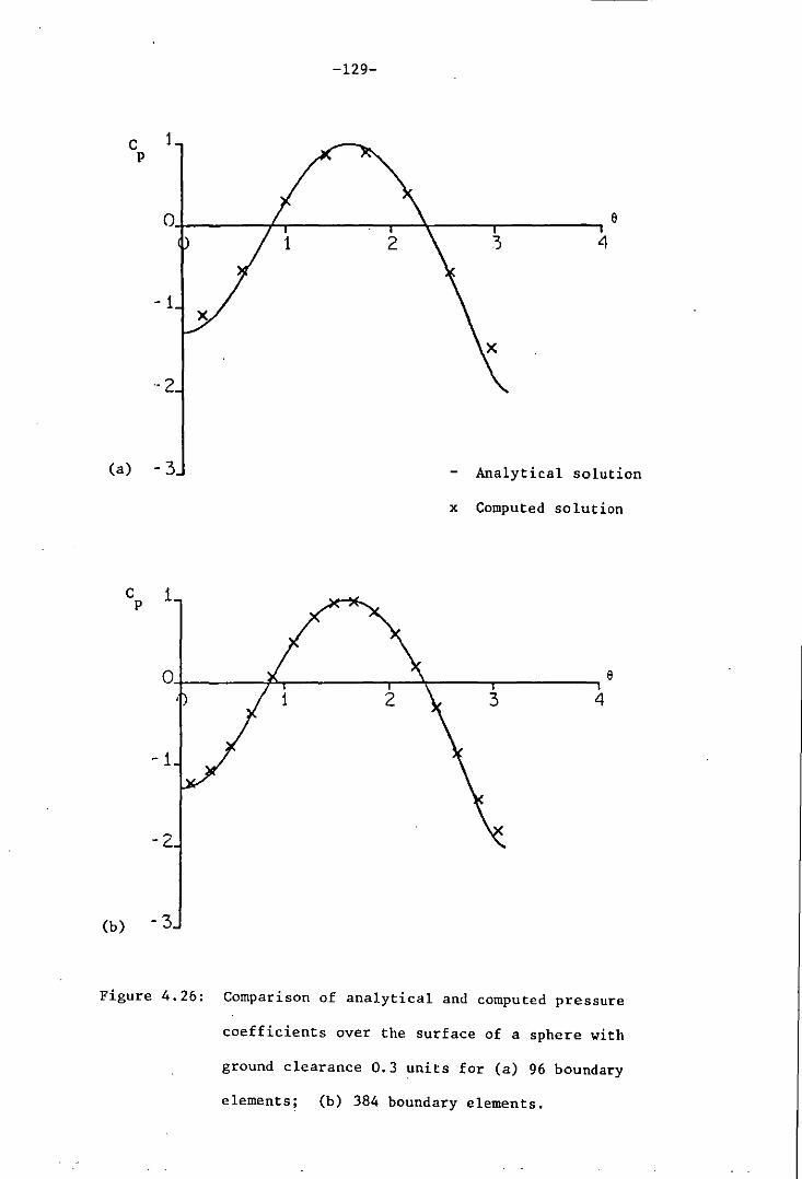
C P

1

-129-

Ol+-____ ~r_----~,_~---.-------,e

- 1

-2

(a) - 3

C 1 p

4

x

Analytical solution

x Computed solution

O+------f~------_r~~---.-------,e 4

-1

-2

(b) - 3

Figure 4.26: Comparison of analytical and computed pressure

coefficients over the surface of a sphere with

ground clearance 0.3 units for (a) 96 boundary

elements; (b) 384 boundary elements.

-130-

IU-LJ.l j

(a)

(b)

Figure 4.27: Discretization of the sphere into 1536 boundary

elements. The point of observation is (a) on

the z-axis; (b) at 45 0 to all axes.

(a) - 5

C 1 p

-131-

6

4

Analytical solution

x Computed solution

O+-----~------_r~----._-----, 6 4

- 1

-2

(b) - 3

Figure 4_28: Comparison of analytical and computed pressure

coefficients over the surface of a sphere for

1536 boundary elements with ground clearance

(a) 0_1 units; (b) 0.3 units.

-132-

I'~==============~~~

(a) '"'=========~~;;:::::::~

(b)

Figure 4.29: Discretization of a semi-infinite body into 48

boundary elements. The point of observation 1S

(a) on the z-axis; (b) at 450 to all axes.

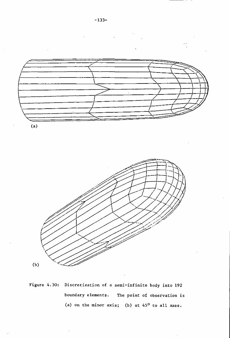
-133-

/ ./ / / :::,.....

I \ \ \ ~~ f \ \ " "" \ ""- \ \ \

----- '\ Y ~ / I

I / I

I /W \" / 7 J ' \ / / \~ -" "- "

(a)

(b)

Figure 4.30: Discretization of a semi-infinite body into 192

boundary elements. The point of observation is

(a) on the minor axis; (b) at 45 0 to all axes.

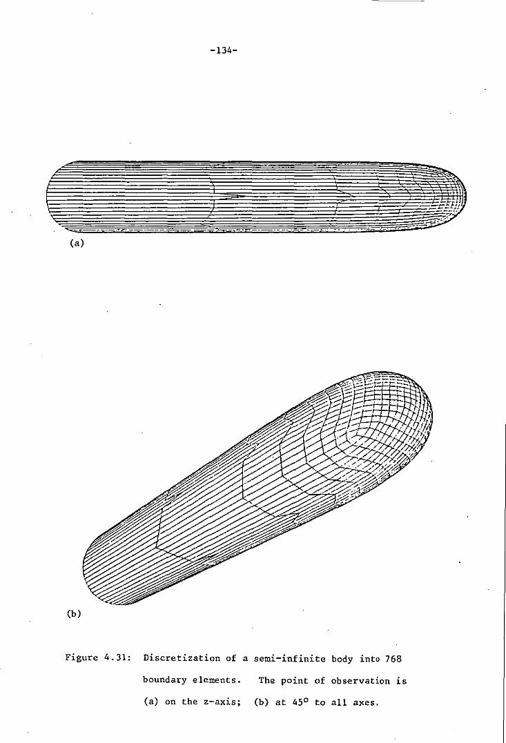
-134-

(a)

(b)

Figure 4.31: Discretization of a semi-infinite body into 768

boundary elements. The point of observation is

(a) on the z-axis; (b) at 450 to all axes.

c p

-135-

5

Ol+-------~._x__r----~~-----. e :3 4 2

-5

Analytical solution

(a) - I a x Computed solution

C P

X 10- 1 10

5

Ol-t----..-J'r-----,,-----x-r-----, e 3 4

-5

Figure 4.32: Comparison of analytical and computed pressure

coefficients on a semi-infinite body using (a) 48

boundary elements; (b) 192 boundary elements.

C P

-136-

Analytical solution

x Computed solution

5 \ 0~ _____ -.~ ___ ---.----~~-----. e

4

-5

-10

Figure 4.33: Comparison of analytical and computed pressure

coefficients on a semi-infinite body using 768

boundary elements.

-137-

SECTION 5

COMPARISON OF THE DIRECT AND INDIRECT

BOUNDARY ELEMENT ~lETHODS

5.1 INTRODUCTION

In this section the indirect boundary element method is discussed

and is applied to obtain the flowfield calculations around the bodies

which were considered in section 4. The results obtained by this

method are compared with those which were obtained using the direct

boundary element method in section 4. In the usual indirect boundary

element method, the surface of the body under consideration is covered

with a distribution of singularities such as sources or doublets and

the· basic unknowns are then calculated in the form of source or

doublet strengths over the body. The calculated singularity

distribution can then be used to calculate the tangential velocity of

the flow over the body. For three-dimensional problems consideration

will be given only to doublet distributions and source distributions

will not be considered, due to the following reasons.

The boundary element methods are to be applied to calculate the

flowfield around road vehicles which generally have some net circulation

of flow around them which gives rise to a lift force on the vehicle.

A source distribution alone cannot produce any circulation and must

therefore be used in conjunction with a doublet distribution. If the

-138-

surface of the body is covered with a source distribution and the wake

surface with a doublet distribution, then, as discussed by Ahmed and

Rucho [14); this representation leads to numerical difficulties at the

end of the body where the wake starts. The problem can be overcome

to some extent by an artificial extension of the wake interior to the

body but this still represents extra complications as compared to the

case for a distribution of doublets alone. Furthermore, if the surface

of the body is covered with a source distribution, then the resulting

matrix of influence coefficients is not always diagonally dominant and

then an iterative method of solution is not possible.

A combined distribution of sources and doublets could be used to

. cover the surface of the body and the wake, which would introduce twice

as many unknowns as compared with the distribution of sources alone or

doublets alone. This technique is often used in two dimensional

aerodynamics, where the extra set of unknowns are eliminated by

equating the strength oJ the singularities on pairs of elements on the

top and bottom surface of the body respectively. This clearly has no

counterpart in three-dimensions, and in any case is essentially aimed

at dealing with sharp trailing edgesof wings, a problem which does

not occur with bluff road vehicles. Thus, keeping in view the above

mentioned difficulties, the surface of the body as well as the surface

of the wake will be covered with a distribution of doublets alone.

In section (5.2), alternative formulations of the indirect

boundary element method in the case of doublet distributions alone are

discussed while the matrix formulation is given in section (5.3). In

section (5.4), the method is applied to calculate the flow past a

circular cylinder, a sphere and ellipsoids of revolution, while in

section (5.5) the flow around the sphere is calculated taking the

-139-

ground effects into consideration. Finally, in section (5.6), the

modelling of the wake is discussed and the method is applied to a

semi-infinite body. The results obtained in section (5.4) to (5.6)

are compared with the corresponding results_in section 4 with regard

to accuracy. The comparison of the computing times for both the

direct and indirect methods is given in section (5.7) and the

conclusions of this chapter are presented in section (5.8).

5.2 ALTERNATIVE FORMS OF THE INDIRECT BOUNDARY ELEMENT

METHOD USING DOUBLET DISTRIBUTIONS

The equation (2.4.4) for the indirect boundary element method in

the case of a doublet distribution alone can be written as

(1 - ci)[~i - ~il + ~i = ~~ - 4~ ff. S-L

a 1 (~' - ~)an ( r )dS

Denoting -(~' - ~) = ~, the strength of the doublet, the above

equation takes the form

~. = $ + (1 - c.)~. 1 co 1 1 + 4~ JJ ~ a (.!.) dS

an r (5.2.1)

S-i

In order to apply the boundary condition of zero normal velocity,

equation (5.2.1) is differentiated with respect to 'n' to give a second

derivative on the R.H.S. In this formulation, the unknowns are

calculated in the form of doublet strengths ~hich-are then used to

calculate the tangential velocity via the derivative of equation

(5.2.1) with respect to 't'. This approach is the 'usual' indirect

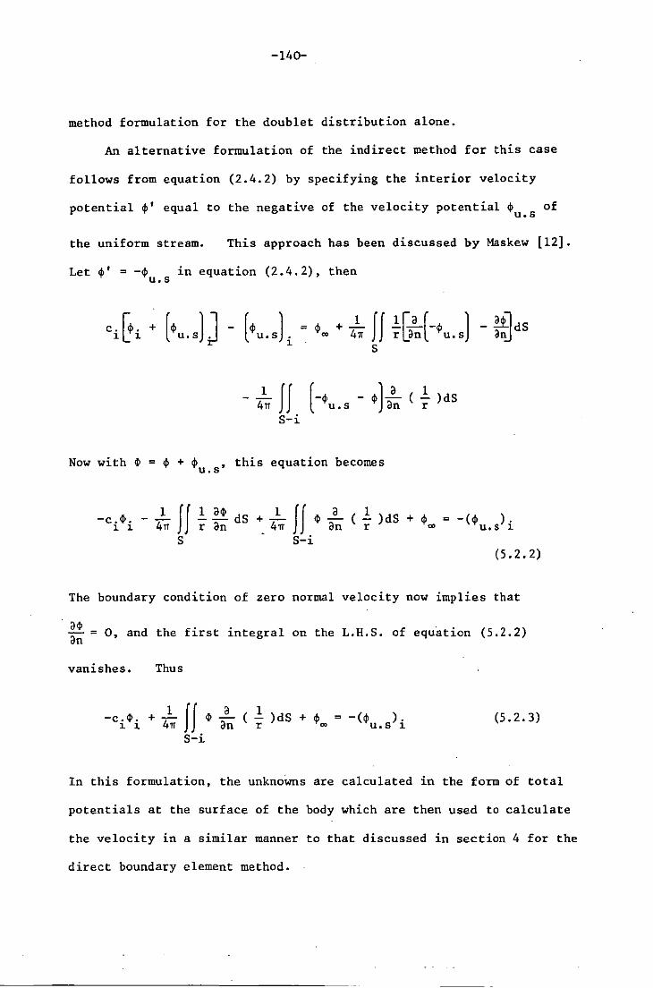
-140-

method formulation for the doublet distribution alone.

An alternative formulation of the indirect method for this case

follows from equation (2.4.2) by specifying the interior velocity

potential ~' equal to the negative of the velocity potential ~ of u.s

the uniform stream. This approach has been discussed by Maskew [12].

Let ~' = -~ in equation (2.4.2), then u.s

c. r~. + 1~ 1

1 ff [-~ - ~)..!.. ( ..!:. )dS 411 u.s an r s-i

Now with ~ = ~ + ~ ,this equation becomes u.s

ff .!. ~ dS + 1 r an 411 ff~ a (.!.) dS + ~

an r co

S S-i

- WdS atU

(5.2.2)

The boundary condition of zero normal velocity now implies that

~ = 0, and the first integral on the L.H.S. of equation (5.2.2) an

vanishes. Thus

a (.!. )dS + ~ = _(~ ). an r tXI u. S 1

(5.2.3)

In this formulation, the unknoWns are calculated in the form of total

potentials at the surface of the body which are then used to calculate

the velocity in a similar manner to that discussed in section 4 for the

direct boundary element method.

-141-

The formulation of the indirect method given by equation (5.2.3)

is much easier to implement than the 'formal' doublet approach and will

be used throughout this section to' calculate the flow field around

three-dimensional bodies.

For two-dimensional problems, the equation of the indirect

boundary element method in the case of a doublet distribution alone

with this formulation takes the form

-c.4>. 1 1

1 +-2IT f

r-i 4> ..2... (log! )dr + ... an r 't'~

5.3 MATRIX FORMULATION

(5.2.4)

In this section the matrix formulation of the equation (5.2.3)

will be discussed. The same procedure can be adopted for the matrix

formulation of the equation (5.2.4). Divide the surface of the body

into m quadrilateral boundary elements, then equation (5.2.3) can be

written as

-c. 4>. 1 1

m +..l. E

4IT j=l If S.-i

J

4> a (! )dS + $ an r co

(5.3.1)

The integrals on the L.H.S. of equation (5.3.l)are of the same form as

the integrals on the L.H.S. of equation (3.3.1) except that $ in the

integrals of equation (3.3.1) has now been replaced by the total

potential 4>. Proceeding as in section (3.3) for the case of exterior

flow problems, equation (5.3.1) in the case of constant, linear or

higher order elements can be expressed in the matrix form as

-142-

[H) {.!!} = {R} (5.3.2)

where as usual [H) is a matrix of influence coefficients, {~} is a

vector of unknown. total potentials ~. and' {R} on the R.H.S. is a 1

known vector whose elements are the negative of the values of the

velocity potential of the uniform stream at the nodes on the surface

of the body. Note the difference in the matrix formulations

(3.3.21) and (5.3.2). In the latter case, the matrix [C) of

influence coefficients on the R.H.S. is absent as opposed to the matrix

formulation (3.3.21) for the direct boundary element method. Again

in the formulation (5.3.2), for the case of linear or higher order

elements, the values of the coefficients in the diagonal of the matrix

[H) can be calculated from the equation (3.3.22), once the off-

diagonal coefficients are all known.

5.4 UNBOUNDED FLOW FIELD CALCULATIONS

In this section, the indirect boundary element method with

formulation (5.2.3) has been applied to calculate the flow past a

circular cylinder, a sphere and ellipsoids of revolution. In the

case of a circular cylinder, the flow is also calculated using the

source distribution alone and a comparison of this formulation with

that of formulation (5.2.3) has been presented. Again the boundary

of the circular cylinder is discretized into the constant and the

linear boundary elements and the integrals over these elements are

calculated numerically using Gauss-quadrature rule with four

integration points except for the element corresponding to the node

under consideration. For this element the integrals are calculated

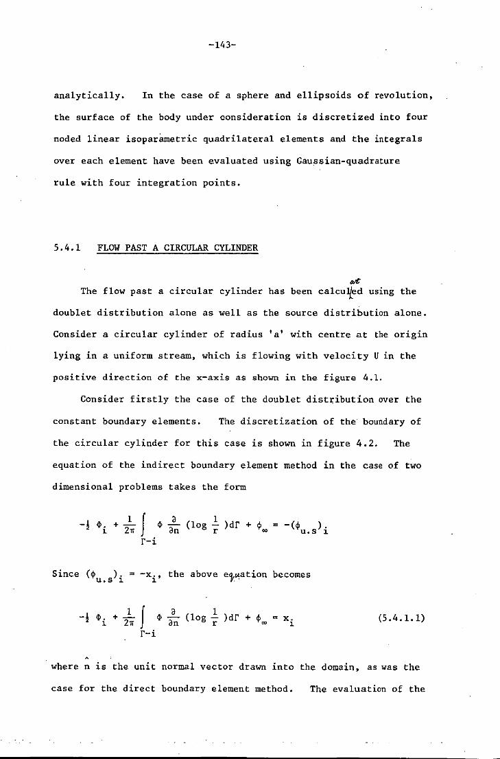
-143-

analytically. In the case of a sphere and ellipsoids of revolution,

the surface of the body under oonsideration is discretized into four

noded linear isoparametric quadrilateral elements and the integrals

over each element have been evaluated using Gaussian-quadrature

rule with four integration points.

5.4.1 FLOW PAST A CIRCULAR CYLINDER

tVt The flow past a circular cylinder has been ca1cu~ed using the

doublet distribution alone as well as the source distribution alone.

Consider a circular cylinder of radius 'a' with centre at the origin

lying in a uniform stream, which is flowing with velocity U in the

positive direction of the x-axis as shown in the figure 4.1.

Consider firstly the case of the doublet distribution over the

constant boundary elements. The discretization of the boundary of

the circular cylinder for this case is shown in figure 4.2. The

equation of the indirect boundary element method in the case of two

dimensional problems takes the form

-! 4>. 1

1 +-2rr I 4> ~ (log! )dr + ~ an r w

r-i

Since (~ ). u.s 1.

-Xi' the above e}~ation becomes

I 4> ~ an r-i

1 (log r )dr + ~w = X.

1 (5.4.1.1)

where n is the unit normal vector drawn into the domain, as was the

case for the direct boundary element method. The evaluation of the

-144-

integrals in equation (5.4.1.1) has already been discussed in section

(4.2.1). Once these integrals are calculated, equation (5.4.1.1) can

now be written in the matrix form (5.3.2) which can be solved for the

total potentials ~ .• 1

Again the velocity at the 8 points shown in

figure 4.4 is calculated using the formula (4.2.1.19). The table (1)

below shows the comparison of the analytical and the calculated

velocities over the boundary of the circular cylinder for 8 points.

Table (1)

x- y- Calculated Analytical

Element Coordinate Coordinate Velocity Velocity

1 -0.79 0.33 0.82884E+00 0.76537E+00

2 -0.33 0.79 0.2001OE+Ol 0.18478E+Ol

3 0.33 0.79 0.200l0E+Ol 0.18478E+0l

4 0.79 0.33 0.82884E+00 0.76537E+00

5 0.79 -0.33 0.82884E+00 0.76537E+00

6 0.33 -0.79 0.2001OE+Ol 0.18478E+Ol

7 -0.33 -0.79 0.200l0E+Ol 0.18478E+Ol

8 -0.79 -0.33 0.82884E+00 0.76537E+00

On comparison of the results of this table with those in table (1) on

page (81), which were obtained using the direct boundary element

method, it is seen that the results obtained with the direct method are

more close to the analytical ones.

Next consider the case of a doublet distribution over linear

boundary elements. The discretization of the boundary of the

circular cylinder into elements is shown in figure 4.5. The

evaluation of the integrals in equation (5.4.1.1) for this case is

-145-

discussed in section (4.2.1) and again equation (5.4.1.1.) can be

put in the matrix form as in equation (5.3.2), which will be

solved for the total potential ~ .• 1

The velocity at the mid-point of

each element, as shown in figure 4.5 is calculated using formula

(4.2.1.19) • The table (2) below shows a comparison of the

analytical and calculated velocities for the 8 boundary elements.

Table (2)

x- y- Calculated Analytical

Element Coordinate Coordinate Velocity Velocity

1 -0.85 0.35 0.71971E+00 0.76537E+00

2 -0.35 0.85 0.17375E+Ol 0.18478E+Ol

3 0.35 0.85 0.17375E+Ol 0.18478E+Ol

4 0.85 0.35 0.71971E+00 0.76537E+OO

5 0.85 -0.35 0.71971E+00 0.76537E+OO

6 0.35 -0.85 0.17375E+Ol 0.18478E+Ol

7 -0.35 -0.85 0.17375E+Ol 0.18478E+Ol

8 -0.85 -0.35 0.71971E+00 0.76537E+OO

On comparison of the results of this table with those in table (3) on

page (88), which were obtained using the direct boundary element method,

it is seen that in this case the results obtained with the indirect

method are more close to the analytical results, in contrast to the

situation for constant elements. Also it can be seen that with this

formulation in passing from constant boundary elements to linear

boundary ele~nts, the accuracy is increased, as one expects. Once

again, an increase in the number of elements leads to an increase in

accuracy.

-146-

Let us now consider the case of a source distribution over the

constant boundary elements. Discretize the boundary of the circular

cylinder as shown in the figure 5.1.

y

Figure 5.1

A n

x

tangent

The equation of the indirect boundary element method for the source

distribution alone in the case of two-dimensional exterior flow problems

can be written as

4>. 1

~ +1:...J 'I'~ 2rr r

( log! )adr r

(5.4.1.2)

In order to apply the boundary condition of zero normal velocity at the

surface, equation (5.4.1.2) is differentiated with respect to 'n' to

give

a 1 an ( log r )dr

If the point 'i' is on the boundary, the integral on the R.H.S.

becomes singular and thus

-147-

f a a ( log.!. ) dr an r

(5.4.1.3)

r-i

where r - i indicates that the point 'i' has been excluded from the

boundary r. In this case, contrary to the direct boundary element

method or the indirect boundary element method with formulation

(5.3.2), n is the unit normal vector to the fixed point 'i' on the

boundary.

The boundary of the circular cylinder is discretized into m

boundary elements, such that equation (5.4.1.3) can be written as

O. + 1

m 1:

j=l t2lrr [,-i J

a 1 an ( log r (5.4.1.4)

since o. are constant over the elements. J

The integrals on the R.H.S. of equation (5.4.1.4) on the elements

are evaluated numerically except for the element on which the fixed

point 'i' is lying. For thi. element the integrals are calculated

analytically. The reason for adopting this choice is that although

in this particular case of constant elements the integrals over all

the elements could be evaluated analytically, in the case of higher

order boundary elements the integrals become too difficult to evaluate

analytically. On the other hand, whilst all these integrals could be

evaluated numerically for any elements, including that over which the

fixed point 'i' is lying, this latter procedure gives poor results.

It will be shown in section (6) that the normal procedure for numerical

evaluation of integrals on the boundary elements for three-dimensional

problems over which the fixed point 'i' is lying gives poor results.

As the integrals cannot be evaluated analytically in that case, an

-148-

alternative quadrature scheme has been developed which gives much

better results.

where

H •. 1J

1

= iw 1 1

Equation (5.4.1.4) then becomes

m E

j=l H .. a.

1J J

r12 [(x. - x ) cos 0( + (y. - y ) s in 0( 1 -29- d(.

1 q 1 q

(5.4.1.5)

in which (x .• y.) are the coordinates of the fixed point 'i' and 1 1

(Xq

' yq) are the coordinates of any general point 'Q' on the element

over which the integration is being performed.

Let H .. = 1J I

' H ..

1J

H •• + ! 1J

when i ;. j

when i = j

then equation (5.4.1.5) takes the form

m E

j=l H ..

1J

which can be expressed in the matrix form

(5.4.1.6)

From this equation the unknowns are calculated in the form of the source

strengths a. over the boundary of the circular cylinder which are then 1

used to find the tangential velocities.

Now the tangential velocity at the mid-point of each element can

be found by differentiating equation (5.4'.1.2) with respect to 't'. thus

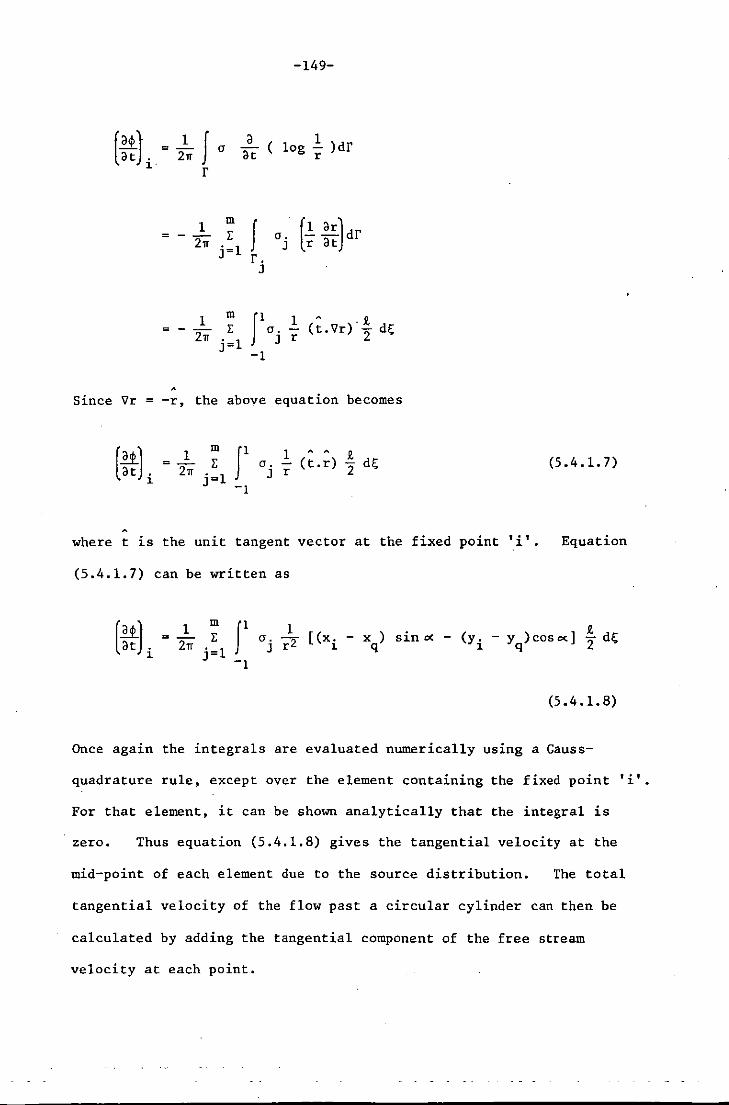
-149-

a 1 at ( log r )dr

m J:...;: 211 • 1

J=

1 A _ t r (t. '7r) "2 d!,;

Since Vr = -r, the above equation becomes

1 m J1 = 2rr ;:

j=l -1

1 ,.. A R. o. (t.r) -2 d!,;

J r (5.4.1.7)

where t is the unit tangent vector at the fixed point , . ,

]. . Equation

(5.4.1.7) can be written as

1 o. -r2 [(x. - x ) J ]. q

sin 0( - (y. - y ) cos 0< 1 ! d!,; ]. q 2

(5.4.1.8)

Once again the integrals are evaluated numerically using a Gauss-

quadrature rule, except over the element containing the fixed point

For that element, it can be shown analytically that the integral is

zero. Thus equation (5.4.1.8) gives the tangential velocity at the

, . , ]. .

mid-point of each element due to the source distribution. The total

tangential velocity of the flow past a circular cylinder can then be

calculated by adding the tangential component of the free stream

velocity at each point.

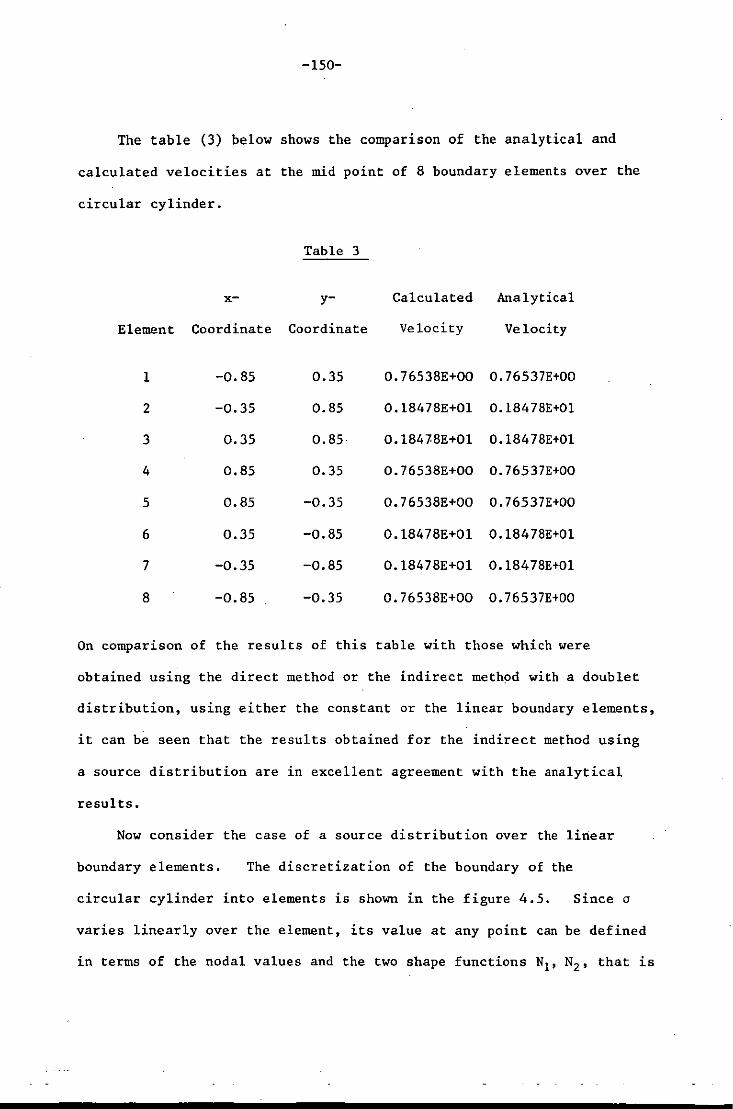
-150-

The table (3) below shows the comparison of the analytical and

calculated velocities at the mid point of 8 boundary elements over the

circular cylinder.

Table 3

x- y- Calculated Analytical

Element Coordinate Coordinate Velocity Velocity

1 -0.85 0.35 0.76538E+00 0.76537E+00

2 -0.35 0.85 0.18478E+Ol 0.18478E+Ol

3 0.35 0.85 0.184'8E+Ol 0.18478E+Ol

4 0.85 0.35 0.76538E+00 0.76537E+00

5 0.85 -0.35 0.76538E+00 0.76537E+00

6 0.35 -0.85 0.18478E+Ol 0.18478E+Ol

7 -0.35 -0.85 0.18478E+Ol 0.18478E+Ol

8 -0.85 -0.35 0.76538E+00 0.76537E+OO

On comparison of the results of this table with those which were

obtained using the direct method or the indirect method with a doublet

distribution, using either the constant or the linear boundary elements,

it can be seen that the results obtained for the indirect method using

a source distribution are in excellent agreement with the analytical

results.

Now consider the case of a source distribution over the linear

boundary elements. The discretization of the boundary of the

circular cylinder into elements is shown in the figure 4.5. since 0

varies linearly over the element, its value at any point can be defined

in terms of the nodal values and the two shape functions NI' N2 , that is

-151-

The detailed formulation follows closely that given for the constant

source distribution. In this particular case, the influence coeffi-

cients matrix with an even number of boundary elements becomes

singular, therefore the tangential velocities at the mid points of 9

boundary elements are calculated. The table (4) below shows the

comparison of the analytical and computed velocities at the mid-points

of 9 boundary elements.

Table 4

x- y- Calculated Analytical ,

Element Coordinate Coordinate Velocity Velocity

1 -0.88 0.32 0.58077E+00 0.68404E+00

2 -0.47 0.81 0.14706E+Ol 0.17321E+Ol

3 0.16 0.93 0.16723E+Ol 0.19696E+Ol

4 0.72 0.60 0.10915E+Ol o .12856E+Ol

5 0.94 0.00 0.40494E-06 O.OOOOOE+OO

6 0.72 -0.60 0.109l5E+Ol 0.12856E+Ol

7 0.16 -0.93 0.16723E+Ol 0.19696E+Ol

8 -0.47 -0.81 0.14706E+Ol 0.1732lE+Ol

9 -0.88 -0.32 0.58077E+00 0.68404E+OO

On comparison of the results of this table with those in table (3)

on page U50). which were obtained using constant boundary elements,

it is seen that the results with linear elements in the source

formulation are poor.

-152-

More importantly, it can be seen that in using a 'usual' indirect

method, after calculating the unknowns in the form of source/doublet

strengths over the body, one has to formulate and ·solve further integrals

to calculate the tangential velocity. This is in contrast with the

formulation (5.2.3 ) of the indirect method with a doublet distribution

where, after finding the unknowns in the form of total potentia1s, one

can easily calculate the tangential velocity by taking the derivative.

Certainly, it is one of the reasons for which the 'usual' indirect

method is rejected.

5.4.2 FLOW PAST A SPHERE

Consider the sphere placed in a uniform stream as shown in the

figure 4.7. Once again the sphere is discretized into 96 and 384

linear boundary elements by the method discussed in section (4.2.2).

Since the uniform stream is in the positive direction of the x-axis,

the velocity potential ~ of the uniform stream is given by u.s

~ = -Ux u.s

-x with U = 1

-x. 1

Thus equation (5.2.3) takes the form

fJ (5.4.2.1)

s-i

The matrix formulation of this equation is discussed in section (5.3).

Since with this formulation the unknowns are calculated in the form of

-153-

total potentials ~., the pressure coefficients at the surface of the 1

sphere are found by the same method as discussed in section (4.2.2).

The pressure coefficients obtained by this method for 96 and 384

boundary elements are again compared with the analytical ones. The

results obtained by this method appear like those shown in figure 4.18

for the direct boundary element method, but are in fact more accurate,

the difference being manifest in the third decimal place of the

solution.

5.4.3 FLOW PAST AN ELLIPSOID OF REVOLUTION

Consider next flow past the ovary ellipsoids (prolate spheroids)

which were discussed in section 4; namely ovary ellipsoids of fineness

ratios 2 and 10, with a distribution of elements as discussed in

section (4.2.3). The tiiscretizations of the ovary ellipsoid of

fineness ratio 2 into 96 and 384 boundary elements are shown in

figures 4.19 and 4.20 respectively, while figures 4.22 and 4.23 show

the discretizations of the ovary ellipsoid of fineness ratio 10 into

96 and 384 boundary elements respectively. The velocity

distributions over the surface of the ovary ellipsoids of fineness

ratios 2 and 10 are calculated using formulation (5.2.3) for 96 and

384 boundary elements and are compared with their analytical solutions.

The results obtained by this method for an ellipsoid of fineness ratio

2 are better than those obtained by using·the direct boundary element

method in the fourth decimal place, whereas the results obtained by

this method for the case of an ellipsoid of fineness ratio 10 become

worse than those obtained by using the direct boundary element method

-154-

in the fourth decimal place. The reason for this could be that the

distribution of elements on the surface of an ellipsoid of fineness

ratio 2 remains almost uniform, whereas in the case of an ellipsoid

of fineness ratio 10, the distribution becomes worse. This situation

agrees with the results of Maskew [12), who has concluded that the

direct method appears to be the most forgiving when faced with poor

element distributions. Since the results obtained by this method for

both ellipsoids differ from results obtained by the direct method only

in the fourth decimal place, their graphical comparison with analytical

results appears the same as that shown for the direct method in

figures 4.21 and 4.24.

5.5 EFFECTS OF A GROUND PLANE

The indirect boundary element method with formulation (5.2.3) has

also been applied to calculate the flow past a sphere in the proximity

of the ground. Consider a sphere of unit radius with centre at the

origin lying near the ground in a uniform stream of velocity U in the

positive direction of the x-axis as shown in figure 4.10. The sphere

is discretized in turn into 96, 384 and 1536 boundary elements as

shown in figures 4.16, 4.17 and 4.27. The pressure coefficients over

the surface of the sphere for 96, 384 and 1536 boundary elements are

calculated once again with ground clearances of 0.1 and 0.3 units.

Since the results obtained by using this method differ in the

second or third decimal place from those which were obtained using the

direct method, their graphical comparisons with the analytical ones

look the same as those shown in figures 4.25, 4.26 and 4.28. It should

-155-

be remembered that the analytical results in the above mentioned

figures, with which the computed results are compared, do themselves

have some error. In general the error is in the fourth decimal place,

but at points very near the ground in the case of ground clearance of

0.1 units, the error could be in the second or even first decimal

place. .The detailed comparison of the computed results obtained

using the direct and the indirect methods with the analytical results

show that the results with the indirect method are close to the

analytical ones at half or slightly more points shown in the above

mentioned figures. Furthermore, the results with the indirect method

are better near the line joining the centres of the spheres, whilst the

results with the direct method are better on the remaining points.

5.6 MODELLING OF A WAKE

The equation (5.2.3) for the indirect boundary element method

holds for an infinite domain surrounding the closed body. In this

section, this equation will again be modified as in the case of the

direct boundary element method to take into account the wake of the

body. Let the body under consideration be as shown in the figure 5.2.

-156-

e

to .. S s.

I

Figure 5.2

The surface of body is S ~ SB + SW + Si, where SB is the surface of the

actual body, Sw the surface of the tubular wake which starts from the

rear end of the body and extends to infinity in the direction of the

onset flow and S~ the surface of that portion of the sphere S* cut 1

by the wake of the body.

Let the surface S divide the space into two regions Rand R' and

let n be the outward drawn unit normal to the surface S. Let tp and tp'

denote the velocity potentia1s of the acyclic irrotationa1 motions in

the regions Rand R' respectively, with ~ regular at infinity. Then

if the point 'i' be internal to R' and therefore external to R, then

from section (4.4) with c. ~ 0, 1

o ~ 2.. II l. 2.t dS 4Tf r an SB

tp ..l.. ( l. )dS an r

(5.6.1)

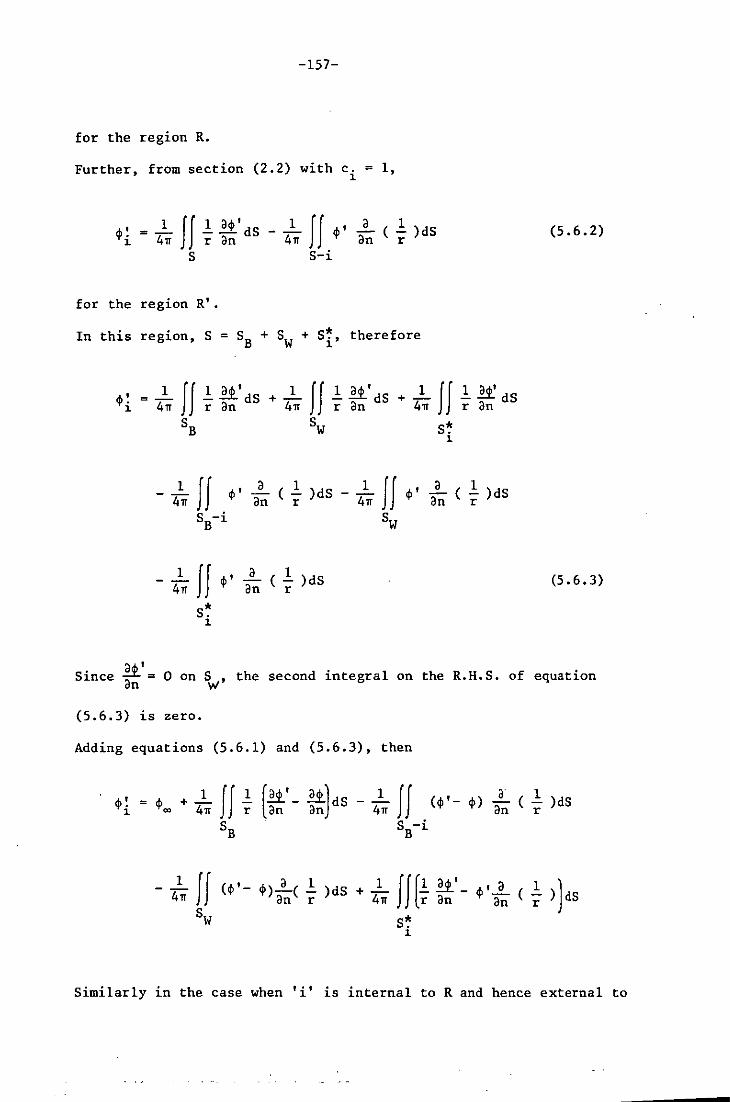
-157-

for the region R.

Further, from section (2.2) with c. ~ 1, ~

<P ~ ~...!.. II .!. ~' dS ~ 4" r an

S

for the region R'.

a (.!.) dS an r

In this region, S ~ S + S + S~, therefore B w ~

1 +-

4" II .!. ~'dS r an

Sw S~ ~

- 4~ If <p' a ( 1 )dS - 4~ If <p' a an r an

S -i B Sw

- 41" If <p '

a ( .!. )dS an r

S~ ~

(5.6.2)

.!. ~ dS r an

( .!. )dS r

(5.6.3)

a'" ' Since ~a = 0 on S , the second integral on the R.H.S. of equation n VI

(5.6.3) is zero.

Adding equations (5.6.1) and (5.6.3), then

<p~ = <p +...!.. II -rl

1 00 4rr SB

«P'- <P)~( .!. )dS + ..!.. II[.!.~'-an r 4" r an Sw S~

~

a ( 1 )dS an r

<p,~ ( 1 an r

Similarly in the case when 'i' is internal to R and hence external to

-158-

R', the same equation results with ~. replacing ~~ on the L.H.S. In 1 1

particular, when 'i' lies on the surface S, then ~~ is replaced by 1

The above mentioned three cases can be combined by

writing

[c.~. + (1 - c.)~~l ~ + 1 If 1 (~'- ~)dS = 4n 11. 1. l. ~ r an an

1 If (4) '- ~) a

- 4n an S -i B

+ 4~ f f (~r.,' - ~' * s. 1

SB

( 1. )dS r

a (l ») dS an r

where c. = 0 when 'i' .is within RI 1

= 1 " " " " "

4~ If w- ~)

Sw

=! when 'i' is on Sand S is smooth.

a ( 1. )dS an r

(5.6.4)

Let the interior velocity potential ~' be equal to the negative

of the velocity potential of the uniform stream, 4> ,then u. s

+...!...ff ~..2.... 411 an ( 1. )dS

r

+...!... 4n

where ~ = 4> + 4> . u.s

a (1.) dS + ...!... an r 4n If [-

* S. 1

S -i B

1 a~u. s r an + 4>u.s

(5.6.5)

The boundary condition of zero normal velocity on the body now implies

-159-

a4> an = 0 on SB' thus the first integral on the R.H.S. becomes zero.

Also the uniform stream in the negative direction of the x-axis has the

velocity potential

cj>u.s = Ux

= x when U = l

* Further, since the outwardly drawn unit normal n to S. is in the 1

a negative direction of the x-axis, then -- = an

on the R.H.S. of equation (5.6.5) becomes

4l~ JI * S. 1

a x -­ax

= 4~ fJ [~+ x r12 ~~)dS * S. 1

~ 0 as -x and r ~ ~.

Hence equation (5.6.5) reduces to

-c.4>. +...!.. JJ 4>.1.. ( 1. )dS +...!.. ]. ]. 4~ an r 4~

S -i B JI Sw

4> a an

= - (cj>u.s)i

:x and the last integral

( ~ )dS + cj>~

(5.6.6)

"On comparison of this equation with that of equation (5.2.3), it

can be seen that now there is an additional integral on the L.H.S of

equation (5.6.6) which is to be evaluated over the surface of the wake.

Equation (5.6.6) can be put in the matrix formulation (5.3.2) by

following the procedure discussed in section(4.4) which can then be

-160-

solved for the unknown total velocity potentials and thus the pressure

coefficients over the surface of the body can be calculated by the same

method outlined in the preceding sections. Again in this case the

wake integral can be evaluated by the method discussed in section (4.4)

and its value turns out to be the same as the value of the wake

integral for the direct method found in section (4.4).

5.6.1 FLOW PAST A SEMI-INFINITE BODY

The equation (5.6.6) for the indirect boundary element method has

been applied to calculate the flow past the semi-infinite body of

figure 4.14. The method of distribution of elements on the semi-

infinite body has been discussed in section (4.4.1). Once again the

semi-infinite body is discretized in turn into 48, 192 and 768

boundary elements as shown in figures 4.29, 4.30 and 4.31 respectively.

The pressure distribution over the surface of the semi-infinite

body has been calculated for each element distribution and the

comparisons with the analytical solutions are shown in figures 5.3

and 5.4. As compared with the direct method, results obtained with

this indirect method are much worse on the elements near the rear end

of the body, but slightly better on the remainder of the body.

Thus it appears that the formulation of the indirect boundary

element method given by Maskew [12] is not suitable for calculating

the flow around bodies having tubular wakes. Maskew only considered

the case of two-dimensional wakes of negligible thickness, shed from

the trailing edge of a wing.

It therefore appears that the direct method is better than the

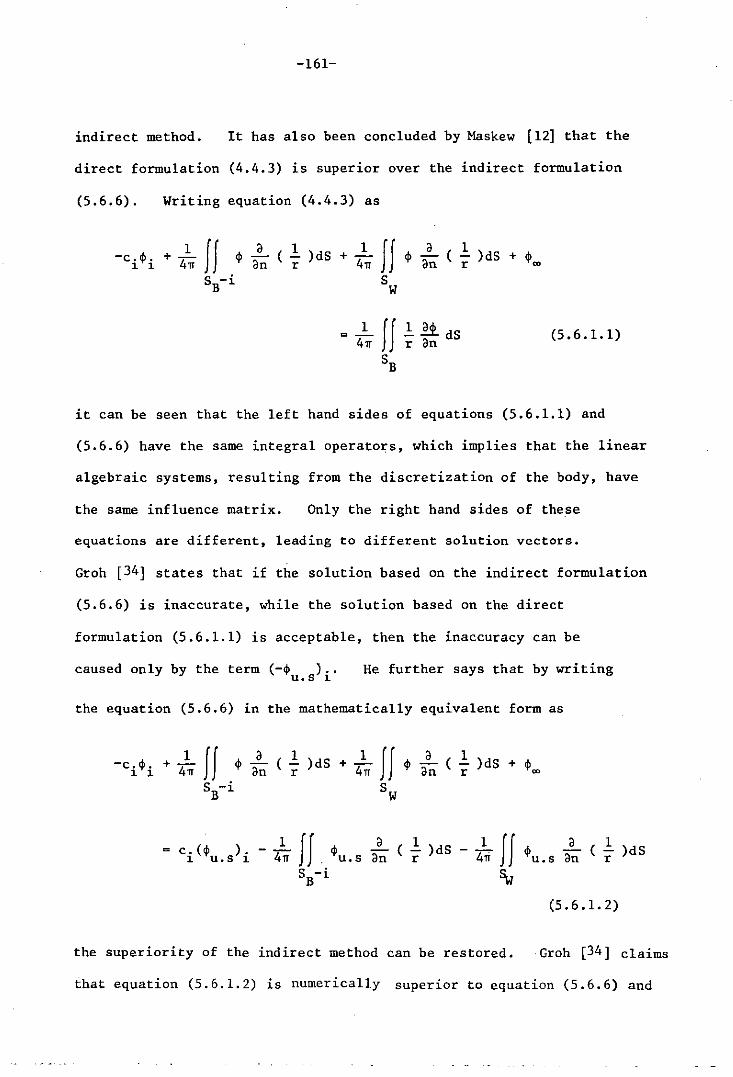
-161-

indirect method. It has also been concluded by Maskew [12] that the

direct formulation (4.4.3) is superior over the indirect formulation

(5.6.6). Writing equation (4.4.3) as

+J:... If <P a

( 1 )dS

1 JJ <P

a ( 1:. )dS + <Pm -ci<Pi +-4" an r 4" an r

S -i S B W

1 JJ 1:. ~ dS (5.6.1.1) =-

4" r an SB

it can be seen that the left hand sides of equations (5.6.1.1) and

(5.6.6) have the same integral operators, which implies that the linear

algebraic systems, resulting from the discretization of the body, have

the same influence matrix. Only the right hand sides of these

equations are different, leading to different solution vectors.

Groh [34] states that if the solution based on the indirect formulation

(5.6.6) is inaccurate, while the solution based on the direct

formulation (5.6.1.1) is acceptable, then the inaccuracy can be

caused only by the term (-<Pu.s)i. He further says that by writing

the equation (5.6.6) in the mathematically equivalent form as

II all

.<p an ( r )dS + 4IT a (1:.) dS + <P an r co

S -1 B

1 IJ =c.(<p )·-4" <P 1 u.s 1 u.s

S -i B

a (1:.) dS an r

the superiority of the indirect method can be restored.

(5.6.1.2)

Groh [34] claims

that equation (5.6.1.2) is numerically superior to equation (5.6.6) and

-162-

even equation (5.6.1.1). The flow past a semi-infinite body was

calculated using equation (5.6.1.2), but the results obtained were

exactly the same as those which were obtained already using the

indirect formulation (5.6.6). This implies that the analysis used

already to calculate the flow past bodies with tubular wakes was correct,

and the poor results near the rear of the body are due to the formulation.

Thus it can be concluded that in this application the indirect

formulation (5.6.6) given by Maskew [12] is not numerically inferior as

compared to the formulation (5.6.1.2). Maskew ~2] makes the valid

assertion that the 'best' formulation is very much problem dependent,

as an 'internal flow' should be chosen which requires the least

perturbation from the applied doublet distribution in a particular case.

5.7 COMPARISON OF COMPUTING TIME

The total computing time taken by the direct or indirect boundary

element method in producing the results is almost the same. About 90

to 95 percent of the total computing time has been utilized in setting

up the influence coefficient matrices, while the remaining 5 to 10

percent is used in reading the data, solving the system of equations,

calculation and writing of the results. It may, however, be mentioned

that the percentage of the total computing time in setting up the two

matrices in the direct method is very nearly the same as the percentage

of the total computing time taken to set up a single matrix in the

indirect method. Furthermore, in order to model the effect of a

boundary layer in future stages of analysis it is necessary to use the

non zero normal velocities over the boundary and then the indirect

-163-

method will also require the same two inflence matrices to be formed and

hence will take the same computing time as that of the direct method.

5.8 CONCLUSIONS

On comparison of the direct boundary element method with the

indirect boundary element method used in this section, it can be

concluded that the indirect method is not suitable for the road

vehicle aerodynamics due to the following reasons:

(i) it gives poor results for the body with a tubular wake near the

rear end of the body

(ii) it is not as forgiving to poor panelling representations as

the direct method

(iii) it is not significantly different in respect of the computing

time required.

Due to the above reasons the direct boundary element method will be

used and analysed in the remaining sections for road vehicle

aerodynamics.

X10- 1 C 10

p

C p

5

-5

-10 (a)

X10- 1 10

5

0

-5

-10 (b)

Figure 5.3 :

-164-

x

a 2 3

x

- Analytical solution

x Computed solution

~

\ \

\v a i

~?3 1 'I

• }It

Comparison of analytical and computed pressure

coefficients on a semi-infinite body using

(a) 48 boundary elenents; (b) 192 boundary

elements.

C P

5

-165-

Analytical solution

x Computed solution

01-----~~--~--~~----_: 4

e

-5 x

-10

Figure 5./4: Comparison of analytical and computed pressure

coefficients on a semi-infinite body using 768

boundary elements.

-166-

SECTION 6

CO~'PAR I SON OF I NTEGRATI ON SCHEMES FOR

VARIOUS TYPES OF ELEf.1ENTS

6.1 INTRODUCTION

This section is devoted to the analysis of the direct boundary

element method for various element types and integration schemes. .The

analysis is carried out by comparing the results of the flow field

calculations around the same three-dimensional bodies which were

considered in sections (4) and (5). The aim of these comparisons is to

establish which integration scheme over which type of element is 'best'

with respect to accuracy for given computing time. The outcome of

these comparisons will then be used to calculate the flow field around

road vehicles.

In section (6.2) modified quadrature formulae for elements with

singularities are discussed and modified integration points and weights

are derived for these elements. The accuracy of the modified

quadrature scheme is checked over a flat square element by evaluating

the integrals of equations (3.3.10) and (3.3.12) and the results are

also compared with those obtained using Gauss-quadrature rule over this

element. In section (6.3) the comparison of the Guass-quadrature and

the modified quadrature is presented over general linear and

quadratic boundary elements. Finally, section (6.4) is given to the

comparison of various types of boundary elements.

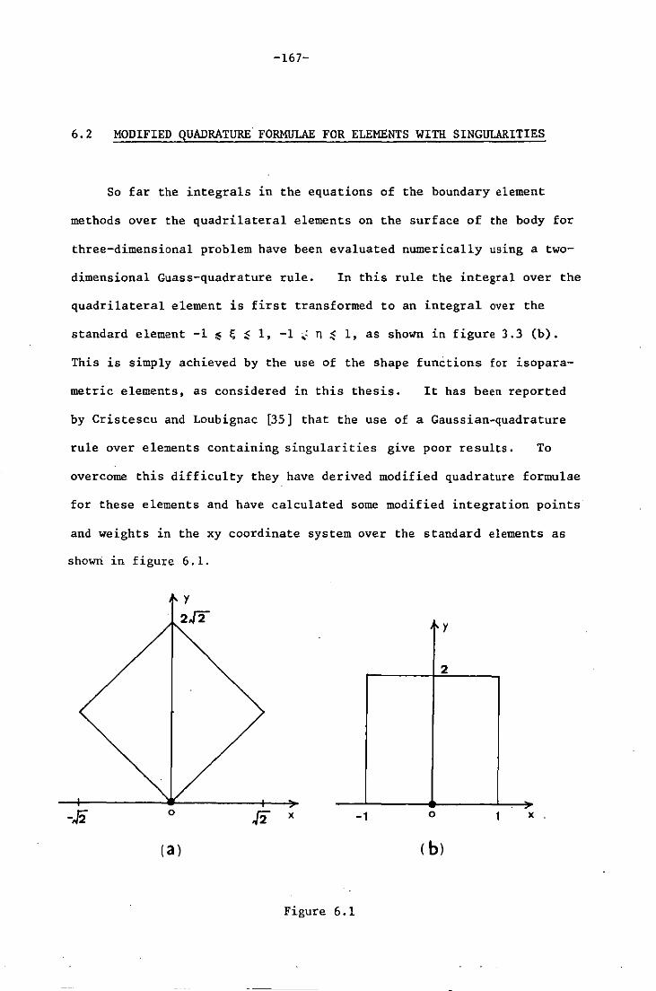
-167-

6.2 MODIFIED QUADRATURE FORMULAE FOR ELEMENTS WITH SINGULARITIES

So far the integrals in the equations of the boundary element

methods over the quadrilateral elements on the surface of the body for

three-dimensional problem have been evaluated numerically using a two-

dimensional Guass-quadrature rule. In this rule the integral over the

quadrilateral element is first transformed to an integral over the

standard element -1 ~ ~ ~ 1, -1 ~ n ~ 1, as shown in figure 3.3 Cb).

This is simply achieved by the use of the shape functions for isopara-

metric elements, as considered in this thesis. It has been reported

by Cristescu and Loubignac [35] that the use of a Gaussian-quadrature

rule over elements containing singularities give poor results. To

overcome this difficulty they have derived modified quadrature formulae

for these elements and have calculated some modified integration points

and weights in the xy coordinate system over the standard elements as

shown in figure 6.1.

2

-,5 o ,[2 x -1 o x

(3) ( b)

Figure 6.1

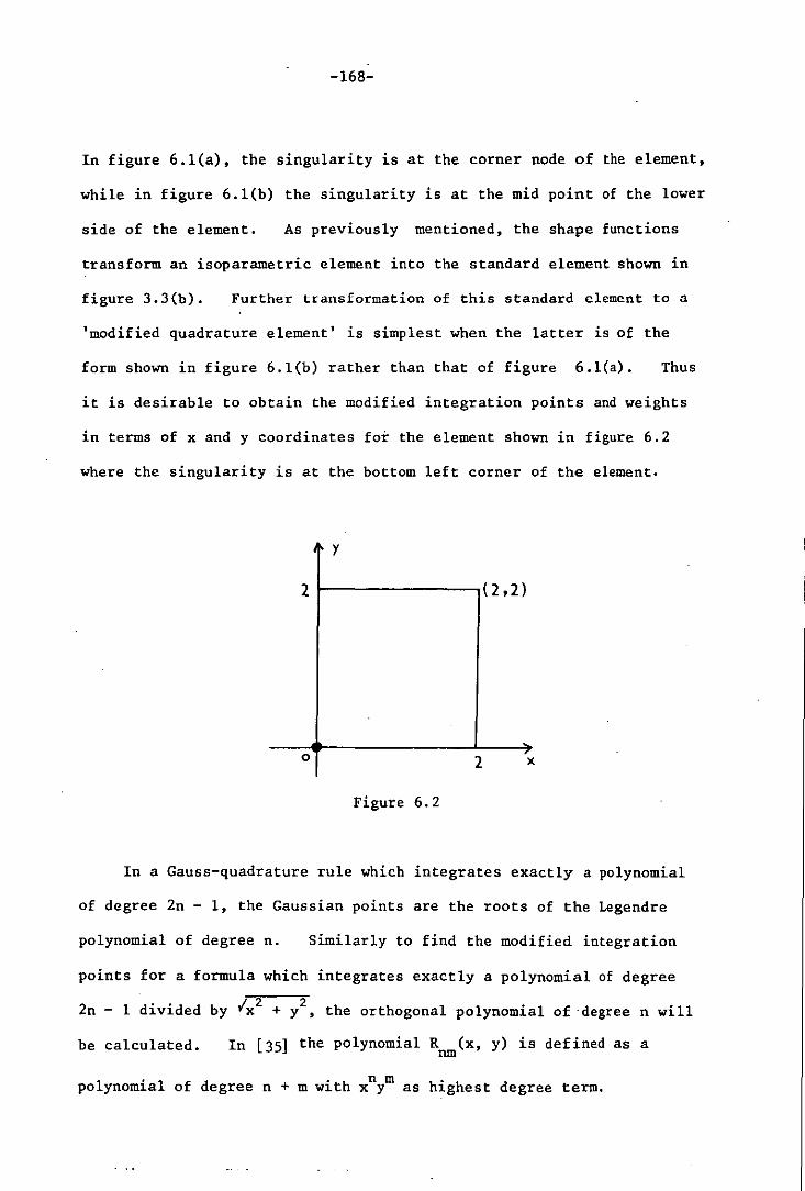
-168-

In figure 6.1(a), the singularity is at the corner node of the element,

while in figure 6.1(b) the singularity is at the mid point of the lower

side of the element. As previously mentioned, the shape functions

transform an isoparametric element into the standard element shown in

figure 3.3(b). Further transformation of this standard element to a

'modified quadrature element' is simplest when the latter is of the

form shown in figure 6.1(b) rather than that of figure 6.1(a). Thus

it is desirable to obtain the modified integration points and weights

in terms of x and y coordinates for the element shown in figure 6.2

where the singularity is at the bottom left corner of the element.

y

2 1-------,( 2,2)

o 2 'x

Figure 6.2

In a Gauss-quadrature rule which integrates exactly a polynomial

of degree 2n - 1, the Gaussian points are the roots of the Legendre

polynomial of degree n. Similarly to find the modified integration

points for a formula which integrates exactly a polynomial of degree

2n - 1 divided by Ix2 + y2, the orthogonal polynomial of ·degree n will

be calculated. In [35] the polynomial R (x, y) is defined as a nm

. . h n m polynomLal of degree n + m WLt x y as highest degree term.

-169-

R (x, y) = xnym + lower order terms run

(6.2.1)

For the four modified integration points the coefficients of R20

(x, y)

and R02

(x, y) need to be calculated, while for the nine integration

points the coefficients of R30 (x, y) and R03

(x, y) will be calculated

and so on. From equation (6.2.1), R (x, y) and R (x, y) can be 20 02

written as

(6.2.2)

The polynomial R (x, y) must be orthogonal to all polynomials of run

degree less than n + m. These conditions give exactly

(n + m)(n + m + 1)/2 equations from which the coefficients of R (x, y) run

can be calculated.

nm Defining x y dxdy

Ix2 + y2 (6.2.3)

the equations determining the coefficients of R20

(x, y) and R02(x, y)

are given in DSJ and thus the four modified integration points are the

common distinct roots of the polynomials R20

(x, y) and R02

(x, y) given

in equation (6.2.2). The four modified integration points for the

element shown in figure 6.2 are given in [35] and the four weights

for this element can be found as follows:

Proceeding as in [35], the four modified weights are calculated from

the equation

-170-

1 1 1 1 "'1 lOO

xl X2 X3 X4 "'2 110

~

x2 1 x2

2 x2 3 x2

4 "'3 120

x3 x3 x3 x3 "'4 130 (6.2.4)

1 2 3 4

where xi' i = 1, ..... , 4 are the modified integration points, wi '

i ~ 1, •..•• , 4 are the unknown modified weights and loo' 110 , 120 ,

130 are defined in equation (6.2.3) and can be found as follows:

(( o 0

1 --;:=;=::::;;: dxd y ,/x2 + y2

Transforming to polar coordinates

loo 2 r/4 f2sec6 drd6

9=0 r~O

~ 4 log (12 + 1 ).

110 (( x dxdy ~

o 0 Ix2 + y2

( ~ (14 + y2 - y)dy 0

2(12 - 1) + 2 log (12 + 1).

120 ~ f( x2

dxdy o 0 Ix2 + y2

-171-

In polar coordinates

130

J1I/4. J2sece

=. r 2cos2e drde +

o 0

8 [11/4 = 3 sec ede 8 J1I

/2

+3 o 11/4

= 1- [12 + log (12 + 1)].

= (( x3 dxdy

o 0 .,Ix2 + y2

( _ l (4 + y2)3/2 = [4.,14 + y2 3

0

= ~ - 4';; + 4 log (12 + 1)

J

2cosece r 2cos2e drde

o .

+ i y3]dy

With these values of loo' 110' 120 , 130 the system of equations (6.2.4)

can be solved and the required modified weights are obtained and are

given in table (1).

Similarly, for nine integration points, the coefficients of

R30 (x, y) and R03 (x, y) need to be calculated, where

(6.2.5)

(6.2.6)

-172-

As in [35] the coefficients of R30 and R03 are calculated from the

following systems of equations respectively.

loo 110 101 120

I I R300 -130 11 02

1 10 120

I 130 I I R301 -140 11 21 12

101 III 102 121 112 103 R302 -I

31 =

120 130 121 I I I R -I 40 31 ,22 303 50

III 121 112 131 I I R -I 22 13 304 41

102 112 10'3 122 113 104 R305 -132

(6.2.7)

lOO 1 10 101 120

I I R -I 11 02 030 03

110 120 III I I I R -I

30 21 12 031 13

101 III 102 I I I R -I 21 12 03 032 04

=

1 20 130 I I I I R -I 21 40 31 22 033 23

III 121 112 I I I R -I 31 22 13 034 14

102 112 103 I I I R -I 22 13 04 - 035 05

(6.2.8)

The elements of the coefficient matrices and that of the R.H.S. vectors

in equations (6.2.7) and (6.2.8) can be found from equation (6.2.3)

giving different values to nand m. lOO. 110. 120 and 130 have

already been found. The remaining elements are found as follows:

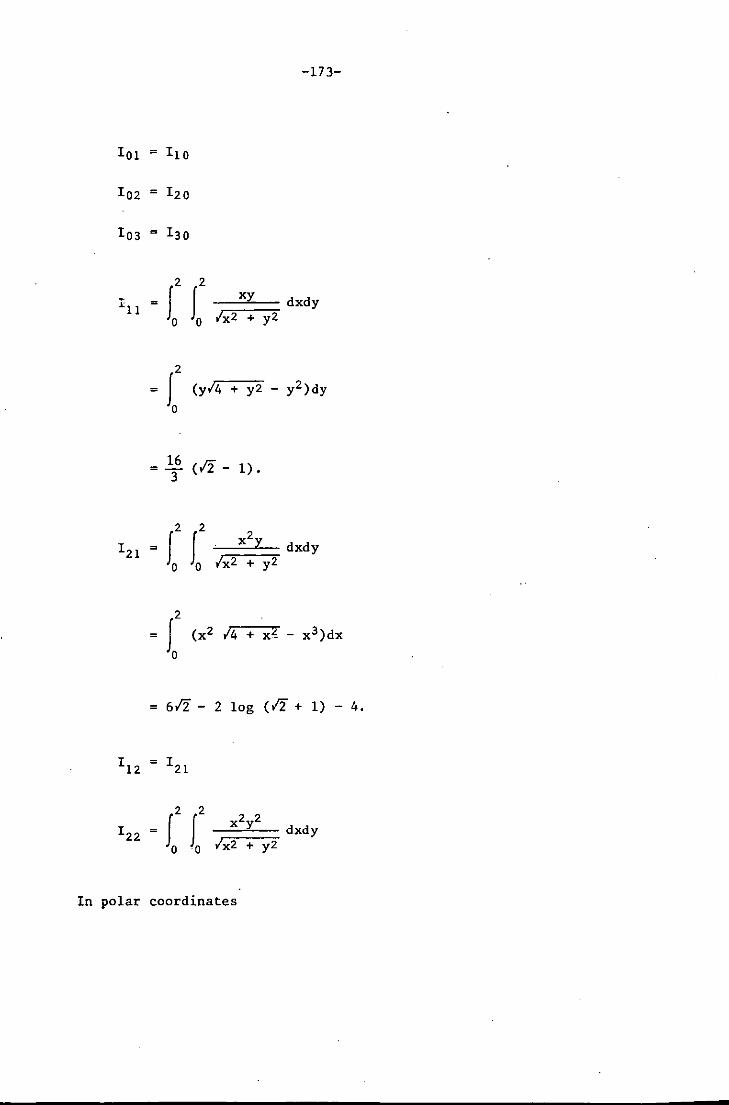
-173-

101 = 110

102 = 120

103 130

III (( xy dxdy

o 0 {x2 + y2

( + y2 - y2)dy = (y{4

0

16 ~ =""3 «2 - 1).

121 = f02 f02 '7-~X=2:::y~;; dxd y {x2 + y2

2

= f (x2 {4 + xg - x 3)dx

o

= 6/2 - 2 log (/2 + 1) - 4.

f 2

f 2

-;:::X;:2=y=2=;: J dxdy o ·0 {x2 + y2

In polar coordinates

-174-

J"/4 J 2sece .

122 = 2 r"cos2e sin2e drde

o 0

-_ 654 J" 14 sin2 e sec 3e de

o

= 3; [12 - log (12 + 1)]

32 = 15 (212 - 1)

I" 0 = J 2

J 2

-;:::.;;:x::"=;;: d xd y o 0 Ix2 + yZ

Transforming to polar coordinates

32 J'Tf/4 = ""5 sec e de

o

32 J'Tf/2 + ""5 cos"e

,,/4

= ~ [11 log (12 + 1) - 12]

J2cosece

r"cos"e drde

o

cosec 5e de

-175-

Transforming to polar coordinates

rr/4 2sece rr/2 2cosece

~

J J r5cos3e sin2e drde +

o 0 f rr/4

f r 5cos3e sin2e drde

o

rr/4

= 32 J sin2 e sec 3e de + "3 o

rr/2

332 f· cos 3e cosec4 e de

rr/4

~ ~6 [1:2 + 4 - 3 log (1:2 + 1)]

14 1 = ( (--;/X::2~X=::::Y=Y:;2 dxd y

Transforming to polar coordinates

rr/4 2sece

J J r 5cos 4 e· sin e drde + o 0

rr/2

J rr/4

rr/4 rr/2

2cosece

J r 5cos4 e o

sine drde

= ~2 J sec e tan e de o

+ 332 f cos4e cosec 5e de

rr/4

2812" 32 = -3- - "3 + 4 log (1:2 + 1).

-176-

ISO = f2 J2 -;:::;::X::s=;: dxdy

o 0 IX2 + y2

In polar coordinates

rr/4 2secS rr/2 2cosecS

t t rScossS drdS + f f rScosSa drdS

rr / 4 0

rr/4

= 332 f sec S dS

o

rr/2

+ 3; f cossS cosec 6S de

rr/4

32 ( ~2 + 1) _ 256 + 22412 = ""3 log, rL 45 45

With these values of loo' •.•.• , Iso' the unknowns in the' systems of

equations (6.2.7) and (6.2.8) which are resp'~ctively the coefficients

in the polynomials R30 and R03 can be, calculated and are given in

table (2). From this table it can be seen that

= R030,

= R03s,

= R031 ]

= R033 (6.2.9)

Having found the unknowns of the systems of equations (6.2.7)and

(6.2.8), the nine integration points are the distinct 32 common roots

of the equations (6.2.5) and (6.2.6). i.e.

(6.2.10)

-177-

and

(6.2.11)

Subtraction of (6.2.11) from (6.2.10) using (6.2.9) gives

(6.2.12)

Addition of (6.2.10) and (6.2.11) using (6.2.9) gives

(6.2.13)

It can be seen that x = y is a root of the equation (6.2.12).

Substituting y = x in equation (6.2.13), then

(6.2.14)

which is a third order polynomial in x.

Let"xI, X2, x3 be the three roots of equation (6.2.14), then

(6.2.15)

are the three modified integration points on the line y = x.

The remaining roots of the equation (6.2.12) are given by

(6.2.16)

From this equation it is not possible to express y explicitly as a

function of x. Therefore, to make this equation easy and

-178-

understandable,transform the xy-coordinate system to the uv-coordinate

system by rotating the axes through 450 anticlockwise as shown in the

figure 6.3.

v

Then u=~+L

and

rz rz

u v x = --rz rz

y = ~ +....::... rz 12

y

u

21-------;((2 . 2)

2 x

Figure 6.3

(6.2.17)

(6.2.18)

Substituting for x and y from equation (6.2.18), equations (6.2.16) and

(6.2.l3) become

(6.2.19)

-179-

'" . 2 2 + ,2 (R303 + R30S)(u + v ) = 0

(6.2.20)

Solving for v2 from equation (6.2.19), then

(6.2.21)

Substituting this value of v 2 into equation (6.2.20), then

(6.2.22)

which is a third order polynomial in u. Le t the three roots of u be

For each of these roots, there are two roots for v from equation

(6.2.21) say ±vl' ±v2' ±v3'

The remaining six modified integration points are given by

These points in the xy-system can be found from equation (6.2.18) which

are given as

-18D-

[~-~, ~+~)

[~+~ ~ , n 12 ~-~)

[~-~, u z + Vz ) 12 12

[Uz Vz Uz Vz) -+-, 12 12 12 12

[~-~, ~ + v3 )

12 12

[ U3 v3 ~-~) +-

12 12 (6.2.23)

Thus the nine modified integration points given in equations (6.2.15)

and (6.2.23) have the values as given in table (3).

Having found these integration points, the nine weights can be

found by solving the following system of equations:

-181-

1 1 · ............. 1 w1 lOO

xl Xz · ............. Xg Wz 1

10

Y1 YZ · ............. Yg w3 101

x 1Y1 xzxz · ............. XgYg w4 III

xZ xZ · ............. xZ w5 I ZO 1 Z 9

yi yZ Z

· ............. yZ 9 w6 IOZ

Z Z Z X1Y1 xZY Z · ............. XgYg w7 121

Z Z Z x 1Y1 xZYZ · ............. XgYg we I 1Z

z z Z z z Z x1Y1 xzYz · ............. XgYg Wg 122

x3 x3 · ............. x3 130 1 2 9

Y~ Y~ · ............. y3 9 103

3 3 3 x1Y1 xzYz · ............. XgYg

131

3 3 3 X1Y1 xzYz · ............. XgYg 1

13

x4 1

x4 Z · ............. x4

9 140

4 Y1

4 Yz · ............. Y~ 104

x 3l x3 y Z 3 z · ............. XgYg 13Z 1 1 Z Z

xZ y3 1 1

xZ y3 2 Z · ............. x2 y 3

9 9 I Z3

4 4 4 x 1Y1 xzYz · ............. XgYg

I 41

4 4 4 x 1Y1 xzYz · ............. XgYg I

14

5 5 5 x x x I 1 Z · ............. 9 50

5 5 y 5 Y1 Yz · ............. 9 I

05 , ,

(6.2.24)

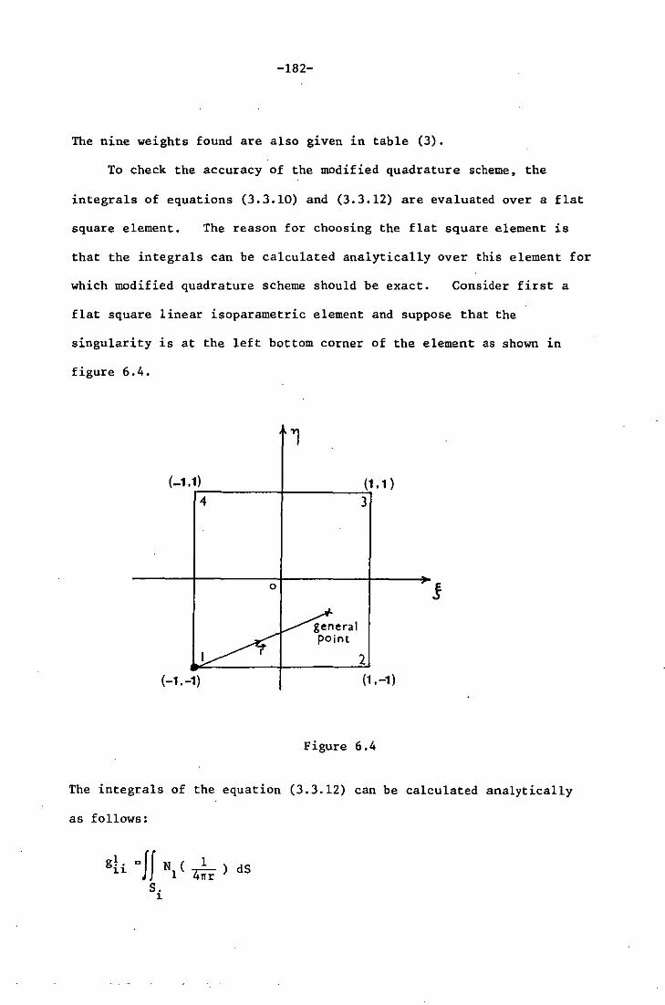
-182-

The nine weights found are also given in table (3).

To check the accuracy of the modified quadrature scheme, the

integrals of equations (3.3.10) and (3.3.12) are evaluated over a flat

square element. The reason for choosing the flat square element is

that the integrals can be calculated analytically over this element for

which modified quadrature scheme should be exact. Consider first a

flat square linear isoparametric element and suppose that the

singularity is at the left bottom corner of the element as shown in

figure 6.4.

'1

(_1,1) (1.1) 4 3

0

I~ ~.eral

pOint

2 (-1.-1) (1.-1)

Figure 6.4

The integrals of the equation (3.3.12) can be calculated analytically

as follows:

gL 11 ~fI N ( 1

1 4iir ) dS

S. 1

-183-

1 1

= __ 1 __ J. J (1 - ~)(1 - n) ~ IGI d~dn 16n r

. -1 _1 .

From figure 6.4, the jacobian IGI = 1 and

r = 1(1 + ~)2 + (1 + n)2

1 1 1 1 J J (1 - 0 (1 - n)

g.. = 1611 -:;:;:;::=:;::::;;:::::::;:;;:::::::;::;;: dE; d n 11 -1 -1 1(1 + E;)2 + (1 + n)2

= 2~ [log (12+ 1) +1 (1- 12)]

Using the value of r from equation (6.2.25) it becomes

1 1

l. = 1!1I J J 11 -1 -1

~=(=l=+~~=)(=l~-=n=)~dE;dn 1(1 + E;)2 + (1 + n)2

1

= 1!1I J (1 - n)[/4 + (1 + n)2 - (1 + n)]dn -1

= 41n [log(12 + 1) + 1 (1 - 12)]

(6.2.25)

4 g ii

1 1

= l!n J J -1 -1

-184-

~~(=l~+~~=)(=l~+=n=)~d~dn 1(1 + ~)2 + (1 + n)2

J

1

- 1 (1 + n)[/4 + (1 + n)2 - (1 + n)]dn - 16n -1

= - 3~ (1 - 12)

J J s.

1

1 1

= l!n J f _1 _1

-;;:;=(::1 ~-~~~)=(l~+~lj=)::;:;;: d~dn 1(1 + ~)2 + (1 + n)2

(1 - ~)[/4 + (1 + ~)2 - (1 + ~)]d~

= 4~ [log(1Z + 1) + i (1 - IZ)]

= 2 g .. 11

The h~. integrals are zero since rand n are orthogonal to each other 11

over this element. The above integrals are calculated numerically

using Gauss-quadrature rule with four, nine and sixteen integration

points as well as using the modified quadrature rule with four and nine

integration points. The comparison of the comp.uted and analytical

-185-

results is shown in table (4). It can be seen from this table that the

results using Gauss-quadrature rule even with sixteen integration points

are not as good as those obtained with the modified quadrature rule

using four integration points. However, the accuracy in the results

with the Gauss-quadrature rule increases with the increase in the

number of integration points, as one would expect. The results

obtained with the modified quadrature rule using four and nine

integration points are exactly the same as those of the analytical

results for this particular element. This is as expected and indicates

that there is no error in formulation of the scheme and that there is

negligible computational error.

Consider next the case of a flat square element with quadratic

functional variation on each side, i.e. an 8 noded square element and

suppose that the singularity is at the bottom left corner of the element

as shown in the figure 6.5.

..,

(-1.1) (0.1) (1 .1)

7 6 5

(-1.0) 8 0 4 (1.0)

1/ lAeneral

pOInt

2 3

(-1.-1) (0.-1) (1. -1)

Figure 6.5

Now the integrals of equation (3.3.12) can be calculated analytically

-186-

as follows:

1 g .. :u

= 1!~ ( ( -1 -1

(1 - ~)(1 - n)(-~ - n- 1) d(dn 1(1 + ~)2 + (1 + n)2

Let 1 + ~ = x and 1 + n = y, then

1 g .. 11

2 2 = __ 1 __ J f (2 - x)(2 - y)(l - x - y) dxdy

16~ o 0 Ix2 + y2

Transforming to polar coordinates, it takes the form

1 1 g .. = 16~

11

rr/2

+ f rr/4

~/4 2secS

[J J. (2 - r· cosS) (2 - r sinS) (1- r cosS - r sinS)drdS o 0

2cosecS t (2 - r cosS) (2 - r sinS) (1 - r cosS - r sinS)drdS ]

rr/4

[J (i secS o

8 - - secS 3

4 sin26) tanS + 3 cos3S dS

~/2

+ f . (i cosecS 8 - - cosecS 3

4 cos2

S) ] cotS + 3 sin3S dS ~/4

= __ 1 __ [4 - 312 + log(12 + 1) 1 12rr

-187-

Z = J J Nz ( 1 ) dS . g .. 411r 1.1. S.

1.

=~ ( ( (1 - E;Z)(l -n) dE;dn 811 1(1 + E;)Z + (1 + n)Z -1 -1

Let 1 + E; = x and 1 + n = y, then

= 8~ ( ( o 0

(2x - x 2 )(2 - y) dxdy

Ix2 + y2

Transforming to polar coordinates,

11 /4 2secS 2 1

g .. = 811 1.1.

[ f J (2 r cosS - r 2cosZe) (2 - r sine)drde o 0

g~. 1.1.

11/2 2cosece

+ J J (2 r cosS - r 2cos2e)(2 - r SinS)drde]

11 /4 0

11/4

= 81

11 [J (~secs o

11/2

+ J ( ~ cosece

11/4

4 - 3 secS tane)de

4 cos 2 e l cotS - 3 sin3e ) d9J

= 2!1I [10 log (12 + 1) + 212 - 4]

= f f N ( 1 ) dS . 3 ~

S. 1.

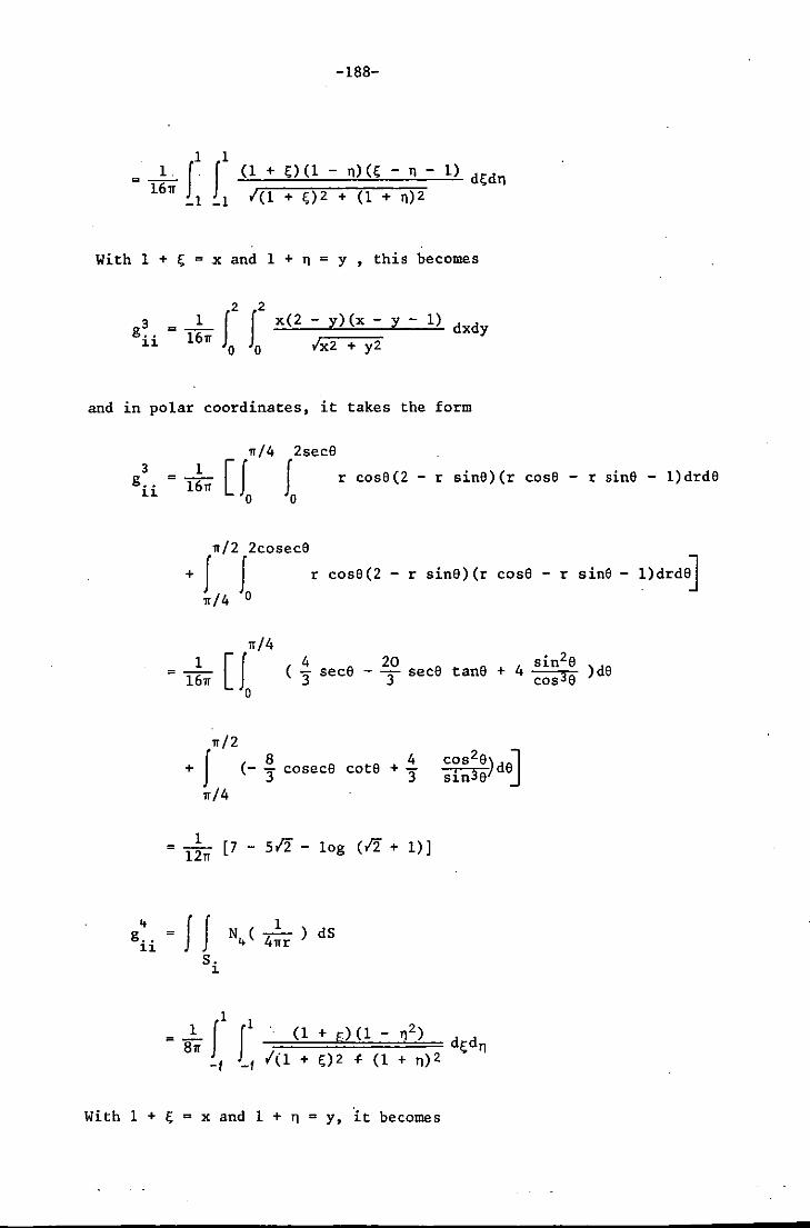
-188-

1 1 = l~n J. J (1 + ~)(1 - 11)(~ - 11 - 1) d~dll

_1 _1 1(1 + 0 2 + (1 + n)2

With 1 + ~ = x and 1 + 11 = Y , this becomes

2 2

= _1 J J x(2 16n

o 0

- y)(x - y - 1) dxdy Ix2 + y2

and in polar coordinates, it takes the form

n/4 2secS

[ J J r cosS(2 - r sinS) (r cosS - r sinS - l)drdS o 0

n/2 2cosecS

+ J J r cosS(2 - r sinS) (r cosS - r sinS - l)drdS]

n/4 0

1 = 16n

n/2

4 20 sin2S ( '3 secS - ""3 secS tanS + 4 cos 3S )dS

+ J (- ~ cosecS cotS +!:. 3

n/4

1 =- [7 - SI2-1og (12+ 1)]

12n

1

= 8~ J r -I -I

-=~(~1=+~f~)(=1==-=11~2~)== ; d~dll 1(1 + ~)2 ~ (1 + 11)2

With 1 + ~ = x and 1 + 11 = y, it becomes

4 g ..

11

-189-

= 8~ J 2

J 2

.::X-";( =2 y;::_::::y;2-:-) dxd y o 0 {x2 + y2

In polar coordinates, it takes the form

rr/4 2secS

g~i = 81rr [t t r cosS (2 r sinS - r 2sin2S)drdS

rr /2 2cosecS

+ J J r cosS(2 r sine - r 2Sin2S)drdS]

rr /4 0

1 = 8rr

rr/4 [J (1; o

rr/2

sin2S secS tanS - 4 cos 3S ) dS

+ f } cosecS cotS dS]

TI /4

1 = 12rr [-10 + 712 + 3 log (12 + 1)]

N ( 1 ) dS 5 4rrr

Let 1 + ~ =·x and 1 + n = y, it becomes

5 g ..

11 - 1

J2 .J2 xy(x + y - 3)

- 16 rr ~O;::;;::::::::;;:-=.!.. d xd Y O {x2 + y2 o .

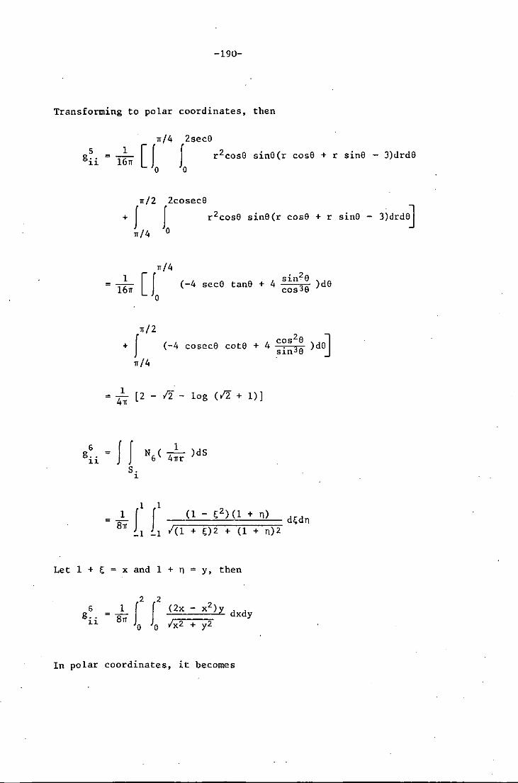
-190-

Transforming to polar coordinates, then

rr/4 2secO

g5 = _1_ [f f r 2cos9 sin9 (r cos9 + r sin9 - 3)drd9 ii 16rr

o 0

rr/2

+ I rr/4

2cosec9

J r2cose o

sine (r cose + r sinS - 3idrde]

sin2e (-4 secS tane + 4 )de cos 3e

rr/2

+ I cos2e ~ (-4 cosece cote + 4 sin3e )dOJ rr/4

1 = 4rr [2 - I'i - log (12 + 1)]

1 Il Il (l - ~2) (l + I) = Brr -;;==;:;:=';==::;=: d~ d I)

_1 -1 1(1 + ~)2 + (1 + n)2

Let 1 + ~ = x and 1 + n = y, then

6 g ..

11 = B~ ( (~(;:2X;:::-=x::;2::-)LY dxdy

o 0 Ix2 + y2

In polar coordinates, it becomes

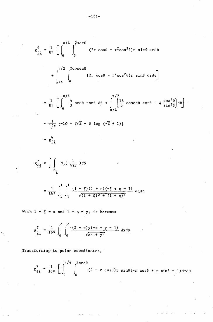
-191-

rr/4 2sec6

6 1 [I I g .. = 8rr 11 0 0

rr/2 2cosece

+ I J (2r

o

1 = 8rr

rr/4

rr/4

[J i o

sece tanG de +

.. /2

I [t36 .. /4

= __ 1 __ [-10 + 71:2 + 3 log (,~ + 1)] 12 ..

7 g ..

11

4 g ..

11

= f I s.

1

cos 2e) ~ cosece cote - 4 sin3e d8J

1 II II (1 - 0 (1 + n) (-~ + n - 1) = --16--.. -I -I -'-".-{~(~l=+ =~;);2;:::+=(~1;::::+~n );=z-;:-=.t... d(; d n

With 1 + ~ = x and 1 + n = y, it becomes

7 g ..

11

= --1!--" J2 J2 --'(.:::.2_----=.x:.<.);.y;( -=x::::+-:;:-y_----=.l.t...) dxdy o 0 Ix2 + y2

Transforming to polar coordinates,

.. /4 2sece

g~i = I!" [f J (2 - r cose)r sine(-r cose + r sinG - l)drdG o 0

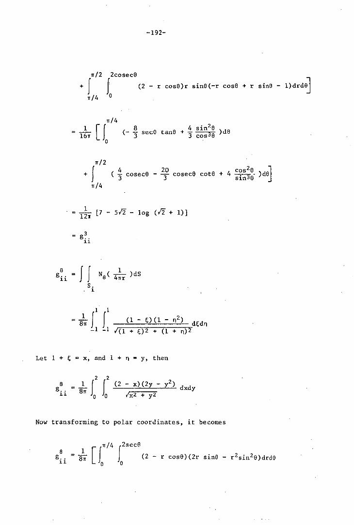
-192-

11 /2 2cosece

+ J f (2 - r cose)r sine(-r co se + r sine - l)drde]

11 /4 0

= 1611

1 8 4 sin2S (- -3 secO tane + - )dS 3 cos 3e

11/2

+ J 4 20 cos2e l ( "3 cosece - ""3 cosece cotS + 4 sin3S' )dSJ

11/4

= 1~1I [7 - 512 - log (12 + 1»)

8 g .. =

11 J J

Let 1 + ~

s. . 1

= 8111 I 1 I 1 ~;-;:::::=:;::;:=;:::==~ (l - ~) (1 - Tj2)

d~dTj _I _I /(1 + ~)2 + (1 + Tj)2

x, and 1 + Tj y, then

2 2

= 81

11 J f (2 o 0

- x)(2y - y2) dxdy

IxZ + yZ

Now transforming to polar coordinates, it becomes

= 1 [fll/4 BiT

o J2sece

(2 o

- r cosO)(2r sinS - r 2sin2S)drdO

-193-

,,/2 2cosece

+ J J (2 - r cose)(2r sine - r 2Sin2e)drde]

,,/4 Q

,,/4 1 [fQ (

8 sec6 tanG - 4 sin2e )de 811 "3 "3 cos3e

,,/2

cosece cote)de] J ( 8 co se cO - 4 + "3 "3

,,/4

= 2!" [10 log (12 + 1) + 212 - 4]

= 2 g .. ~~

k Again the h integrals of equation (3.3.10) are zero, since rand n are

ii orthogonal over this element. The above eight integrals were calculated

numerically using Gauss-quadrature rule with four, nine and sixteen

. integration points as well as using modified quadrature rule with four

and nine integration points. The comparison of the computed and

analytical values of these integrals is shown in table (5). It can be

seen from this table that the same type of behaviour is observed in the

results for this element as was observed for the four noded flat square

element. Once again it can be concluded th.at the weights anu points

for the modified quaurature rule have been evaluated correctly. The

same techni.que could be used to evaluate the integrals having a

singularity of A £n them, but in this work the above formulae have r

k k been used to evaluate the h .. integrals as well as g .. integrals.

11 11

k This has been done becall se the integrand in the case of h .. contains an

LL

-194-

n.r term in the numerator which tends to zero as r approaches zero,

1 thus the overall singularity is effectively that of -r

6.3 COMPARISON OF GAUSS-QUADRATURE AND MODIFIED QUADRATURE SCHEMES

In section 4, the flow field calculations for the sphere,

ellipsoids of fineness ratios 2 and 10, sphere in the proximity of the

ground and the semi-infinite body were obtained using Gauss-

quadrature rule with four integration points. The surface of each

of these bodies was discretized into linear quadrilateral boundary

elements. In this section, the flow field calculations around the

above mentioned bodies are obtained using Gauss-quadrature rule with

nine and sixteen integration points as well as using the modified

quadrature rule with four and nine integration points. The se bod ie s

will be discretized into linear and quadratic isoparametric quadri-

lateral elements. The number of elements and the method of

distribution of these elements for each of these bodies is the same as

discussed in section 4. Tables (6) and (7) show the comparison of

the Gauss-quadrature and th~ modified quadrature rule for 96 and 384

linear boundary elements respectively, while tables (8) and (9) show

the comparison of these two quadrature rules for 96 and 384 quad-ratic

boundary elements respectively. It should be noted that the semi-

infinite body only has half as many elements as all the other bodies

in each table. In the cases of a sphere, a sphere in the proximity of

the ground and the semi-infinite body, the results are compared for the

pressure distributions, while in the case of ellipsoids or'revolution,

the results are compared for the velocity distributions. Furthermore,

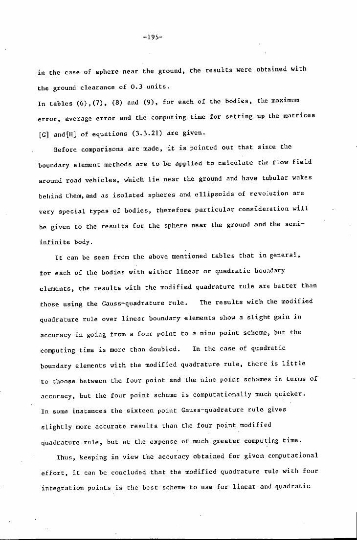
-195-

in the case of sphere near the ground, the results were obtained with

the ground clearance of 0.3 units.

In tables (6),(7), (8) and (9), for each of the bodies, the maximum

error, average error and the computing time for setting up the matrices

[G] and [11] of equations (3.3.21) are given.

Before comparisons are made, it is pointed out that since the

boundary element methods are to be applied to calculate the flow field

around road vehicles, which lie near the ground and have tubular wakes

behind them, and as isolated spheres and ellipsoids of revolution are

very special types of bodies, therefore particular consideration will

be given to the results for the sphere near the ground and the semi­

infinite body.

It can be seen from the above mentioned tables that in general,

for each of the bodies with either linear or quadratic boundary

elements, the results with the modified quadrature rule are better than

those using the Gauss-quadrature rule. The results with the modified

quadrature rule over linear boundary elements show a slight gain in

accuracy in going from a four point to a nine point scheme, but the

computing time is more than doubled. In the case of quadratic

boundary elements with the modified quadrature rule, there is little

to choose between the four point and the nine point schemes in terms of

accuracy, but the four point scheme is computationally much quicker.

In some. instances the sixteen point Gauss-quadrature rule gives

slightly more accurate results than the four point modified

quadrature rule, but at the expense of much greater computing time.

Thus, keeping in view the accuracy obtained for given computational

effort, it can be concluded that the modified quadrature rule with four

integration points is the best scheme to use for linear and quadratic

-196-

boundary elements.

6.4 COMPARISON OF TYPES OF ELENENTS

In this section comparison of different types of boundary elements

will be presented. For this purpose, in this section the flow field

calculations around the bodies considered in section (6.3) are also

obtained using cubic boundary elements. The integrals over the cubic

elements are evaluated numerically using Gauss-quadrature rule with

four, nine and sixteen integration points. The surface of the sphere

and the ellipsoids of revolution will be discretized into 96 cubic

boundary elements, whereas the surface of the semi-infinite body will

be discretized into 48 cubic boundary elements. The me thod of

distribution of elements is the same as discussed in section 4.

On comparison of the results over 96 quadratic boundary elements

in table (8) with those over 96 cubic boundary elements in table (10),

it can easily be seen that the results over the cubic elements are in

general worse than those for the quadratic elements. In particular,

the results for the semi-infinite body in the case of cubic elements

are very poor. The average error and the maximum error increases

with the increase in the number of integration points on the element.

These worse results are on the elements near the rear end of the body.

Furthermore the computing time in the case of cubic elements is more

than double the computing time for the quadratic elements. Hence

quadratic elements are to be preferred to cubic elements on the

grounds both of accuracy and computing time.

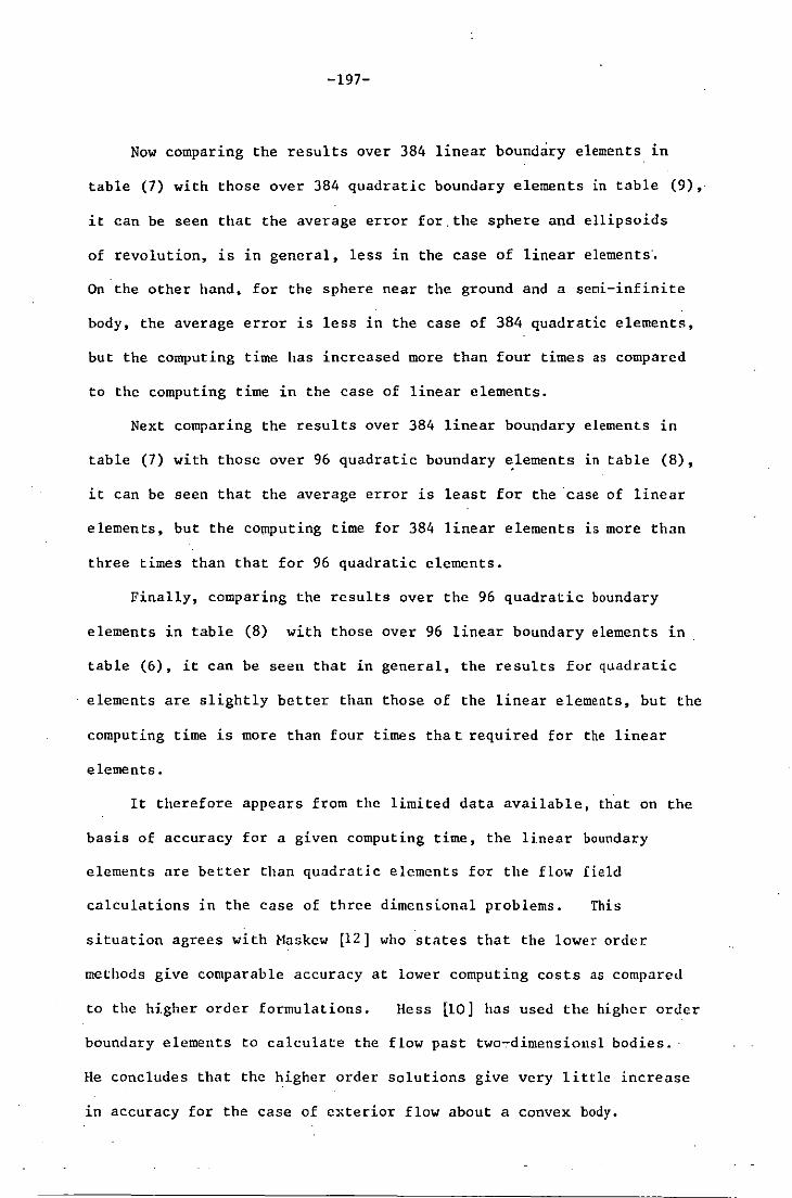
-197-

Now comparing the results over 384 linear boundary elements in

table (7) with those over 384 quadratic boundary elements in table (9),"

it can be seen that the average error for" the sphere and ellipsoids

of revolution, is in general, less in the case of linear elements".

On the other hand. for the sphere near the ground and a semi-infinite

body, the average error is less in the case of 384 quadratic elements,

but the computing time has increased more than four times as compared

to the computing time in the case of linear elements.

Next comparing the results over 384 linear boundary elements in

table (7) with those over 96 quadratic boundary ~lements in table (8),

it can be seen that the average error is least for the case of linear

elements, but the computing time for 384 linear elements is more than

three times than that for 96 quadratic elements.

Finally, comparing the results over the 96 quadratic boundary

elements in table (8) with those over 96 linear boundary elements in

table (6), it can be seen that in general, the results for quadratic

elements are slightly better than those of the linear elements, but the

computing time is more than four times that required for the linear

elements.

It therefore appears from the limited data available, that on the

basis of accuracy for a given computing time, the linear boundary

elements are better than quadratic elements for the flow field

calculations in the case of three dimensional problems. This

situation agrees with Haskew [12] who states that the lower order

methods give comparable accuracy at lower computing costs as compared

to the higher order formulations. Hess [10] has used the higher order

boundary elements to calculate the flow past two-dimensionsl bodies.

He concludes that the higher order solutions give very little increase

in accuracy for the case of exterior flow about a convex body.

-198-

TABLE (1)

MODIFIED WEIGHTS

W1 = 1. 599081

Wz = w4 = 0.624407

w3 = 0.677597

TABLE (2)

COEFFICIENTS OF R30 COEFFICIENTS OF R03

R300 = -0.211575005921497 R030 = -0.211575005921497

R301 = 1.969454455252099 R031 = -0.104865856848484

R302 = -0.104865856848484 Ron = 1.969454455252099

R303 = -2.805208321585304 ROB = 0.029785120454849

R304 = 0.046559886100398 R034 = 0.046559886100398

R305 = 0.029785120454849 R035 = -2.805208321585304

TABLE (3)

MODIFIED INTEGRATION POINTS

xl = 1.711823931756158 YI = xl

Xz

= 0.875937756252321 YZ = Xz

x3 = 0.141101627021577 Y3 = x3

x4

= 0.897460382010956 Y4

= 1.745327820461991

Xs = Y4 Ys = x 4

x6 = 0.198000853722974 Y6

= 1.7500504036~6516

x 7 = Y6 Y7 = x6

Xs = 0.1848800785Z8939 Ye = 0.911042111294785

Xg = Ye Yg = Xa

------

HODIFIED WEIGHTS

wI

= 0.187442978417879

Wz

= 0.666750710927685

w3 = 0.845686715223277

w4 = 0.273178975447147

Ws w4

w6 = 0.168998274274658

w7 = w6

we = 0.470629721991967

Wg = wa

... ..., ..., I

INTEGRAL

1 g ..

n

2 4 g .. , g ..

1.1. 1.l.

3 g ..

n

-----

TABLE (4)

CO~WARISON OF THE GAUSS-QUADRATURE AND THE MODIFIED QUADRATURE

SCHEMES OVER A FOUR NODED FLAT SQUAlrn ELEMENT

GAUSS-QUADRATURE HODIFlED QUADRATURE

4 Points 9 Points 16 Points 4 Points 9 Points

0.1006484 0.1108358 0.1142003 0.1183003 0.118300'3

0.0606223 0.0595966 0.0593198 0.0591501 0.0591501

0.0443786 0.0439831 0.0439595 0.0439494 0.0439494

ANALYTICAL

0.1183003

0.0591501

0.0439494

-----

I

'" o ?

INTEGRAL

1 g .. 11

2 8 gii' g ..

11

3 7 g ..•

11 g ..

11

" 6 gii' g ..

u

5 g •.

11

TABLE (5)

COMPARISON OF THE GAUSS-QUADRATURE AND THE MODIFIED QUADRATURE

SCHEMES OVER AN EIGHT NODED FLAT SQUARE ELEMENT

GAUSS-QUADRATURE MODIFIED QUADRATURE

4 Points 9 Points 16 Points 4 Points 9 Points

-0.0068654 0.0076111 0.0121403 0.0169429 0.0169429

0.1075138 0.1032247 0.1020600 0.1013574 0.1013574

-0.0281349 -0.0258322 -0.0254658 -0.0252643 -0.0252643

0.0700006 0.0676330 0.0675111 0.0674715 0.0674715

-0.0256220 -0.0236499 -0.0235516 -0.0235221 -0.0235221

ANALYTICAL

0.0169429

0.1013574

-0.0252643

0.0674715

-0.0235221

I

'" o .... I

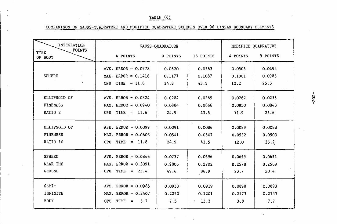
TABLE (6)

COMPARISON OF GAUSS-OUADRATURE AND MODIFIED QUADRATURE SCHEMES OVER 96 LINEAR BOUNDARY ELEMENTS

~ GAUSS-QUADRATURE MODIFIED QUADRATURE

TYPE POINTS OF BODY 4 POINTS 9 POINTS 16 POINTS 4 POINTS 9 POINTS

AVE. ERROR = 0.0778 0.0620 0.0563 0.0505 0.0495

SPHERE MAX. ERROR = 0.1418 0.1177 0.1087 0.1001 0.0983

CPU TIME = 11.6 24.8 43.5 12.2 25.3

ELLIPSOID OF AVE. ERROR = 0.0324 0.0284 0.0269 0.0262 0.0255

FINENESS MAX. ERROR = 0.0940 0.0884 0.0866 0.0850 0.0843

RATIO 2 CPU TIME = 11.6 24.9 43.5 11.9 25.6

ELLIPSOID OF AVE. ERROR = 0.0099 0.0091 0.0086 0.0089 0.0088

FINENESS MAX. ERROR = 0.0603 0.0541 0.0507 0.0532 0.0503

,RATIO 10 CPU TIME = 11.8 24.9 43.5 12.0 25.2

SPHERE AVE. ERROR = 0.0846 0.0737 0.0696 0.0659 0.0651

NEAR THE MAX. ERROR = 0.3091 0.2806 0.2702 0.2578 0.2569

GROUND CPU TIME = 23.4 49.6 86.9 23.7 50.4

SEMI- AVE. ERROR = 0.0985 0.0933 0.0919 0.0898 0.0893

INFINITE MAX. ERROR = 0.2407 0.2250 0.2201 0.2173 0.2133

BODY CPU TIME = 3.7 7.5 13 .2 3.8 7.7

I N o N I

TABLE (7)

COMPARISON OF GAUSS-QUADRATURE MID MODIFIED QUADRATURE SCHEMES OVER 384 LINEAR BOUNDARY ELEMENTS

~ GAUSS-QUADRATURE MODIFIED QUADRATURE

POINTS TYPE .

4 POINTS 9 POINTS 16 POINTS 4 POINTS 9 POINTS OF BODY

AVE. ERROR = 0.0347 0.0257 0.0224 0.0203 0.0191

SPHERE MAX. ERROR = 0.1215 0.0919 0.0801 0.0913 0.0773

CPU TIME = 169.9 362.1 634.1 175.3 369.9

ELLIPSOID OF AVE. ERROR = 0.0097 0.0079 0.0072 0.0068 0.0065

FINEtfESS MAX. ERROR = 0.0387 0.0360 0.0351 0.0336 0.0337

RATIO 2 CPU TIME = ·169.2 360.6 632.8 173.9 366.4

. ELLIPSOID OF AVE. ERROR = 0.0051 0.0042 0.0041 0.0045 0.0040

FINENESS HAlL ERROR = 0.0986 0.0904 0.0876 0.0879 0.0852

RATIO 10 CPU TIME = 171. 7 366.6 641.2 175.4 369.3

SPHERE AVE. ERROR = 0.0320 0.0270 0.0253 0.0239 0.0235

NEAR THE MAX. ERROR = 0.1472 0.1319 0.1264 0.1184 0.1186

GROUND CPU TIME = 347.9 728.0 1273.4 350.9 731.2

SEMI- AVE. ERROR = 0.0304 0.0284 0.0278 0.0258 0.0264

INFINITE HAX. ERROR = 0.0789 0.0663 0.0627 0.0617 0.05S3

BODY CPU TIME = 47.5 100.7 176.6 48.9 102.0 I

I N o '" I

TABLE (8)

COMPARISON OF GAUSS-QUADRATURE AND MODIFIED QUADRATURE SCHEMES OVER 96 QUADRATIC BOUNDARY ~LE~ffiNTS

~ GAUSS-QUADRATURE MODIFIED QUADRATURE

POINTS TYPE

4 POINTS 9 POINTS 16 POINTS 4 POINTS 9 POINTS OF BODY

AVE. ERROR = 0.0519 0.0453 0.0327 0.0229 0.0319

SPHERE MA..'C. ERROR = 0.1111 0.1340 0.0652 0.0404 0.0796

CPU TIME = 50.9 108.7 190.5 52.3 111.0

ELLIPSOID OF AVE. ERROR = 0.0204 0.0265 0.0127 0.0186 0.0180

FINENESS MAX. ERROR = 0.0521 0.0698 0.0368 0.0505 0.0466

RATIO 2 CPU TIME = 50.8 108.5 189.5 52.0 111.1

ELLIPSOID OF AVE. ERROR = 0.0122 0.0149 0.0074 0.0138 0.0090

FINENESS MAX. ERROR = 0.0501 0.0499 0.0399 0.0566 0.0325

RATIO 10 CPU TIME = 51.2 109.3 159.6 52.1 109.1

SPHERE AVE. ERROR = 0.0566 0.0603 0.0498 0.0485 0.0586

NEAR THE MAX. ER.'tOR = 0.1887 0.1153 0.1439 0.0784 0.1011

GROUND CPU TIME = 102.1 218.8 376.6 103.7 219.9

SEm- AVE. ER.'tOR = 0.0551 0.0313 0.0438 0.0582 0.0160

INFINITE MAX. ERROR = 0.1924 0.0394 0.1410 0.1843 0.0173

BODY CPU TIME = 14.9 31.6 53.4 15.3 32.1

I

'" o ..,. I

TABLE (9)

COHPARISON OF GAliss-QUADRATURE AND MODIFIED QUADRATURE SCHEMES OVER 384 QUADRATIC BOlmDARY ELEMENTS

~ GAUSS-QUADRATURE MODIFIED QUADRATURE

POINTS TYPE

4 POINTS 9 POINTS 16 POINTS 4 POINTS 9 POINTS OF BODY

AVE. ERROR = 0.0362 0.0310 0.0209 0.0195 0.0210

SPHERE MAle. ERROR = 0.1126 0.1530 0.0709 0.0863 0.0991

CPU TIME = 779.3 1632.3 2651. 2 785.9 1641. 3

ELLIPSOID OF AVE. ERROR = 0.0132 0.0154 0.0063 0.0102 0.0108

FINENESS MAX. ERROR = 0.0421 0.0752 0.0288 0.0460 0.0512

RATIO 2 CPU TIME = 774.1 1636.0 2863.6 792.2 1646.7

ELLIPSOID OF AVE. ERROR = 0.0056 0.0093 0.0035 0.0073 0.0064

FINENESS MAX. ERROR = 0.0718 0.0861 0.0511 0.0777 0.0572

RATIO 10 CPU TIME = 778.7 1637.8 2860.9 779.9 1649.9

SPHERE AVE. ERROR = 0.0263 0.0184 0.0195 0.0160 0.0197

NEAR THE MAX. ERROR = 0.1213 0.05 0.095 0.053 0.0703

GROUND CPU TIME = 1526.1 3275.0 5693.9 1546.1 3293.9

SEHI- AVE. ERROR = 0.0250 0.0227 0.0189 0.0209 . 0.0164

INFINITE MAX. ERROR = O. 099l 0.1384 0.0666 0.1055 0.0867

BODY CPU TUlE = 206.3 442.1 767.9 211.9 447.8

I N o V> I

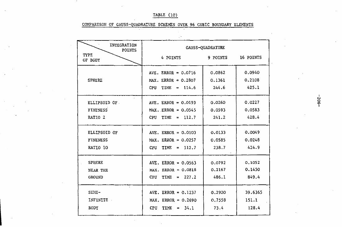
TABLE (10)

COMPARISON OF GAUSS-QUADRATURE SCHEMES OVER 96 CUBIC BOUNDARY ELEMENTS

~ GAUSS-QUADRATURE POINTS

TYPE 4 POINTS 9 POINTS 16 POINTS OF BODY

AVE. ERROR = 0.0716 0.0862 0.0940

SPHERE MAX. ERROR = 0.2807 0.1361 0.2108

CPU TINE = 114.6 244.6 425.1

ELLIPSOID OF· AVE. ERROR = 0.0193 0.0260 0.0227

FINENESS MAX. .ER..'l.OR = 0.0545 0.0593 0.0583

RATIO 2 CPU TIME = 112.7 241.2 428.4

ELLIPSOID OF AVE. ERROR = 0.0103 0.0133 0.0049

FINENESS MAX. ERROR = 0.0257 0.0585 0.0248

RATIO 10 CPU TIME = 112.7 238.7 424.9

SPHERE AVE. ERROR = 0.0563 0.0792 0.1052

NEAR THE MAX. ERROR = 0.0818 0.2167 0.1450

GROUND CPU TL'IE = 227.2 486.1 849.4

SE}!I- AVE. ERROR = 0.1237 0.2920 39.6365

INFINITE MAX. ERROR = 0.2690 0.7558 151.1

BODY CPU TIME = 34.1 73.4 128.4

I N o a­I

-207-

SECTION?

APPLICATION TO ROAD VEHICLES

7.1 INTRODUCTION

In this section the direct boundary element method with linear

quadrilateral elements and using the modified quadrature rule with four

integration points will be used to calculate the pressure distributions

over the surfaces of models of road vehicles. The calculated pressure

coefficients will be compared with the experimental pressure

coefficients which were obtained in wind tunnel tests on models of three

different shapes of car bodies. The experimental work was commissioned

some years ago by BL Technology Ltd. and was carried out at Imperial

College, London.

7.2 COMPARISON OF EXPERIMENTAL AND COMPUTED PRESSURE COEFFICIENTS

OVER THE SURFACE OF A MODEL CAR BODY

The shapes of the car bodies for which the experimental results are

available are of the following types:

(i) car body with vertical back

(H)

(Hi)

"

"

"

"

"

"

short taper

long taper

-208-

See figure 7.1.

Each of the models of the car bodies is simplified in that there were

no wheels, wheel cavities, bumpers and mirrors etc. The experimental

results over the model of each of these types of car bodies were

obtained in a wind tunnel measuring 1.2 meters by 1.37 meters at a

test velocity of 20 meters per second. The wind tunnel had a moving

ground plane which also ran at 20 meters per second. The ground

clearance for each of the models of these three shapes was l8mm, with

the underside set parallel to the ground. Each of the models of the

car bodies has been discretized into linear quadrilateral boundary

elements. The boundary condition of zero normal velocity at the

surface of the car body has the form

n.i (7.2.1)

where the unit normal n can be found by the same method as discussed in

section (4.4.1).

z

164 mm

o ---""'7'-----, ./' // 120mm

+- - --.-

~-j----~

, o o o

---;-­, , ,

- 318 mm­

vertical back-

short taper -

~ - . - - - - - - - . - - • - - • long taper ____ _

y

Figure 7.1

+--

+0-

--u X ----- -)0 --~ +-

-)0

- '-l>

-209-

It should be noted that the plane of symmetry for the car bodies shown

in figure 7.1 has been taken as the xz-plane rather than the xy-plane

as used in previous sections.

and are of 20mm radius.

The edges of the car bodies are rounded

In order to make the comparisons easy, the top, side and bottom

views of each of the types of car body are shown in figure 7.6. In

this figure different lines have been drawn along which the experimental

and computed results will be compared. The lines, A, B, C and D in

the top view are the lines in the planes y = 0, y = 40, y = 50 and

y = 76 respectively. The corresponding lines in the above mentioned

planes in the bottom view have been indicated by A', B' • C' and D'

respectively.

Consider now in turn each of the above mentioned types of car body.

(i) CAR BODY WITH VERTICAL BACK

Consider first the model of the car body which is cut at x = -lOmm

to give a bluff tailed shape. Figures 7.2 and 7.3 show the discretiza-

tion of this car model into L,64 linear quadrilateral boundary elements.

The pressure coefficient at the mid-point of each quadrilateral element

is calculated by the method discussed in section (4). Interpolation

is used to obtain the calculated pressure coefficients at any intermed-

iate points. Figures 7.7 to 7.10 show the comparisons of the

experimental and the computed pressure coefficients over the surface

of the car body with a vertical back. Figure 7.7 shows the

comparisons along the lines A and A', while figure 7.8 shows the

comparisons along the lines B, C and B', C'. In figure 7.8 the graphs

for the experimental and computed results are shown to be discontinuous,

indicating that the deht-most portions of the graphs are the

-210-

comparisons along the lines C and C' and the 1eft-most portions of the

graphs are the comparisons along the lines Band B I • Similarly,

figure 7.9 shows the comparisons along the lines D and D' and figure

7.10 shows the comparison along the line E. In all these figures,

there is quite good agreement between the experimental and the

computed results. In figure 7.10 there is some doubt about the

experimental values in the middle of the body, but the computed results

seem to be consistent.

(ii) CAR BODY WITH SHORT TAPER

Consider next the model of the car body with a 25 0 slant back

which is cut off to give a bluff base of half model height. Figure 7.4

shows the discretization of this model into ·610 linear quadrilateral

boundary elements. Again the pressure coefficient is calculated at

the mid-point of each quadrilateral element and interpolated as

required. Figures 7.11 to 7.14 show the comparisons of the

calculated and experimental pressure coefficients over the surface of

the car body with short taper. In all the figures showing the

comparisons on the top surface of the car body, it can be seen that

there is excellent agreement between the experimental and computed

results except over the slant-back part of the body, where the computed

results differ from the experimental results. This situation might

be due to the separation of the boundary layer from the body, because

in obtaining the results for the car bodies it was assumed that the

boundary layer remains attached right to the rear end of the body.

Even if the boundary layer does remain attached, it will be

considerably thicker here than elsewhere, and the computed results at

present ignore the displacement effects of boundary layer growth. On

-211-

the other hand, for the results on the bottom surface of the body in

these figures, where the boundary layer was always attached and of

small displacement thickness, there is an excellent agreement between

the experimental and the computed results right from the front to the

rear end of the body. In figure 7.12 (b), the second experimental

value from the left seems to be incorrect as noted by the

experimentors. Finally, figure 7.14 shows the comparison along the

line E. Again, as in the case of the car body with a vertical back,

the experimental value near the middle of the body seems to be

incorrect, possibly due to a faulty pressure tapping.

(iii) CAR BODY WITH LONG TAPER

Lastly consider the model of the car body with a 250 slant back

which continues to a point. The boundary layer on the upper surface

is not likely to remain attached right up to the trailing edge of the

body, and the experimental results show the pressure coefficient tending

towards a constant value near the rear of the body, as happens in an

area of separated flow • Therefore, in this case the car body shape

. was truncated at x = -21Smm and then it was assumed that a tubular wake

emanated from this position. Figure 7.5 shows a discretization of

this model car body into 750 linear quadrilateral boundary elements.

The pressure distribution is calculated at the mid-point of each

quadrilateral element. Figure 7.15 to 7.18 show the comparisons of

the experimental and computed pressure coefficients over the surface of

the car body with long taper. It can be Seen from these figures that

the same type of behaviour in the results is observed as was observed in

the case of a car body with short taper.

-212-

* * *

Thus far, in producing the results shown in figures 7.7 to 7.18

over the models of the car bodies shown in figure 7.1, it was assumed

that the tubular wake behind the body starte'd illllIlediately from the rear

end of the body. It can be seen from the results for a car body with

a vertical back from figures 7.7 to 7.10, that near the rear of the

body, the computed pressure coefficient is greater than the

experimental pressure coefficient. This shows that the computed

velocity is less than that of the experimental at the rear of the body.

A complete analysis including the effects of the boundary layer and the

wake should remove this discrepancy between the experimental and

computed results over the rear portion of the car body. The reason

for this discrepancy could be that the wake for the computed results

has been assumed to be parallel to the x-axis immediately from the rear

end of the body, while in reality there would be a slight contraction

of the wake at the rear of the body which would give rise to higher

velocities over the rear portion of the body than would be predicted

from parallel flow. To check the validity of this argument, it was

decided to model a slight contraction of the wake, starting from the

rear end of the body, as a part of the actual body, followed by a

normal tubular wake parallel to the x-axis. This guessed portion of

the flowfield was also discretized into elements in the same manner

in which the actual body was discretized. The pressure distribution

over the surface of the car body with a vertical back was again

obtained. The results obtained for this case are shown in figure 7.19

to 7.22. On comparison of these results with those in figures 7.7 to

-213-

7.10, it can be seen that the results in this case show a behaviour in

the right direction as expected.

Next, consider the case of a car body with a short or long taper.

In this case it can be seen from figures 7.11 to 7.14 or 7.15 to 7.18

that at the rear of the body the difference in the experimental and the

computed pressure coefficients on the top surface of the body is of

greater magnitude than on the bottom surface of the body, in

comparison to the case of a car body with a vertical back where this

difference was of the same order of magnitude on all sides of the body.

In the present case, the experimental and the computed pressure

coefficients are in good agreement on the bottom surface of the body,

while they are much different on the slant back part on the top surface

of the body. The reason for this is that in the case of the computed

results, the velocity distribution is that for potential flow about two

sharp corners which gives rise to large velocities at the expansion

corner and low velocities at the contraction corner, where the tubular

wake is assumed to begin. In reality, the boundary layer and wake

separation effects would produce a much smoother expansion and contraction

of the flow, which would give rise to less extreme values of pressure

coefficient as·is observed in the experimental results.

Figure 7.2: Discretization of the car body shape with vertical back into 464 boundary elements.

Top view.

I N ... ... I

Figure 7.3: Bottom view of the car body shape with vertical back.

I N .... I.n I

Figure 7.4: Discretization of the car body shape with short taper into 618 boundary elements. Top View.

I N ..... a­I

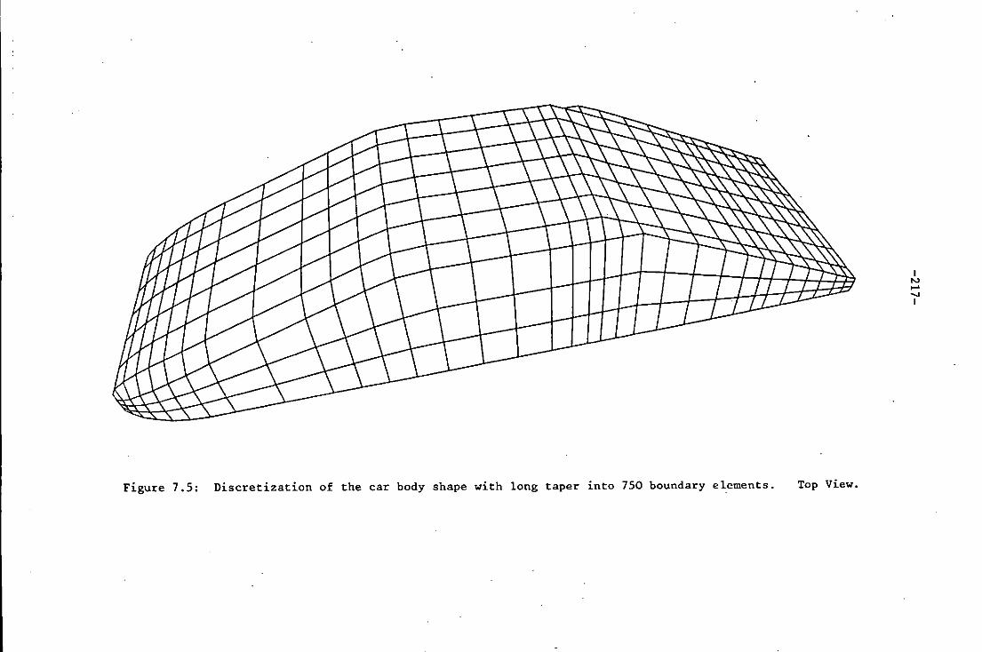
Figure 7.5: Discretization of the car body shape with long taper into 750 boundary elements. Top View.

I

'" .... ..... I

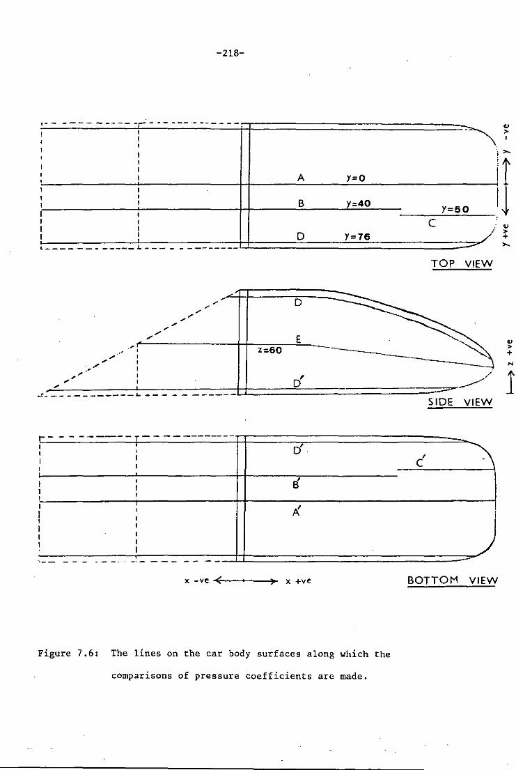
-218-

~- -- --- ------~ - - - - - ------

r-- - - -- 'T

rf, , C

I It !

,{

x -ye .. <~---~)~ x +ye BOTTOM VIEW

Figure 7.6: The lines on the car body surfaces along which the

comparisons of pressure coefficients are made.

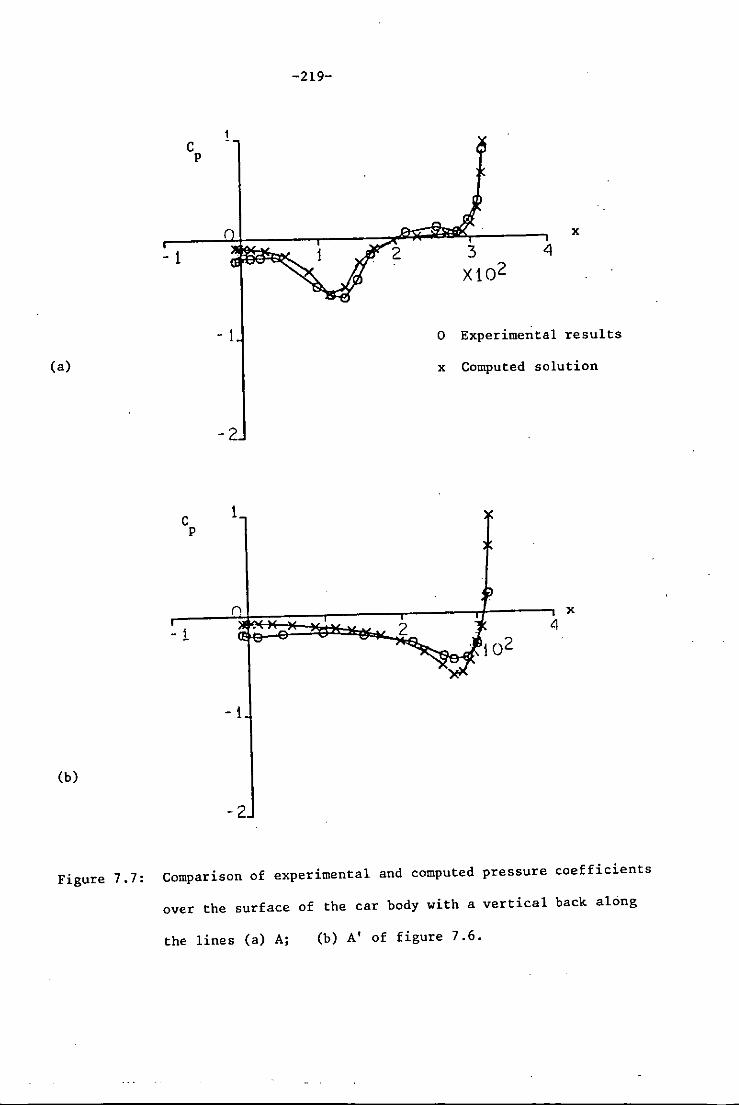
(a)

(b)

- 1

C P

C P

- i

1

- 1

1

- 1

-2

-219-

3 Xl02

x

o Experimental results

x Computed solution

x 4

Figure 7.7: Comparison of experimental and computed pressure coefficients

over the surface of the car body with a vertical back along

the lines (a) A; (b) A' of figure 7.6.

(a)

(b)

- 1

C P

C P

- 1

1

B

- 1

-2

1

- 1

-2

-220-

C

x 2 4

o Experimental results

x Computed solution

C'

x 4

B'

Figure 7.8: Comparison of experimental and computed pressure coefficients

over the surface of the car body with a vertical back along

the lines (a) Band C; (b) B'and C' of figure 7.6.

(a)

(b)

-1

C .p

C P

- 1

1

-1

1

n

- 1

-2

-221-

x

2 4

o Experimental results

x Computed solution

x 4

Figure 7.9: Comparison of experimental and computed pressure coefficients

over the surface of the car body with a vertical back along

the lines (a) D; (b) D' of figure 7.6.

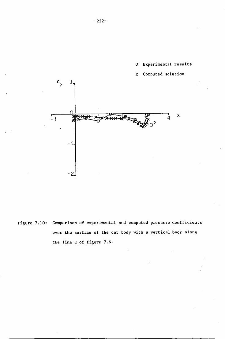
-1

C 1 p

-1

-2

-222-

o Experimental results

x Computed solution

4 x

, 0 2

Figure 7.10: Comparison of experimental and computed pressure coefficients

over the surface of the car body with a vertical back along

the line E of figure 7.6.

-2

(a)

-2

. (b)

C P

C P

-223-

x

o Experimental results

x Computed solution

-2

1

x 4

- 1

Figure 7.11: Comparison of experimental and computed pressure coefficients

over the surface of the car body with short taper along the

lines (a) A; (b) A' of figure 7.6.

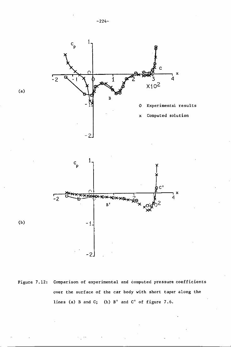
-2

(a)

(b)

C P

C P

1

-2

1

-1

-2

-224-

C x

4

o Experimental results

x Computed solution

r C'

Figure 7.12: Comparison of experimental and computed pressure coefficients

over the surface of the car body with short taper along the

lines (a) Band C; (b) B' and C' of figure 7.6.

-2

(a)

-2

(b)

C 1 p

-2

C 1 p

n

- 1

-2

-225-

x

1 2 4

o Experimental results

x Computed solution

x

4 2

Figure 7.13: Comparison of experimental and computed pressure coefficients

over the surface of the car body with short taper along the

lines (a) D; (b) D' of figure 7.6.

-226-

1

-2

- i

-2

o Experimental results

x Computed solution

x 4

""EJ,~2

Figure 7.14: Comparison of experimental and computed pressure coefficients

over the surface of the car body with short taper along the

line E of figure 7.6.

-3

(a)

-3 -2

(b)

C P

-227-

1

-2

C 1 p

- 1

-2

2 3 X102

4 x

o Experimental results

x Computed solution

x

4

Figure 7.15: Comparison of experimental and computed pressure coefficients

over the surface of the car body with long taper along the lines

(a) A; (b) A' of figure 7.6.

-3

(a)

-3 -2

(b)

-228-

C 1 p

C P

-2

1

-1

-2

x 4

B

o Experimental results

x. Computed solution

C'

x 4

B'

Figure 7.16: Comparison of experimental and computed pressure coefficients

over the surface of the car body with long taper along the

lines (a) Band C; (b) B' and C' of figure 7.6.

-3

(a)

-3

(b)

-2

C P

C P

-229-

1

-2

1

- 1

-2

x

1 12 4 , ,

o Experimental results

x Computed solution

x 4

Figure 7.17: Comparison of experimental and computed pressure coefficients

over the surface of the car body with long taper along the

lines (a) D; (b) D' of figure 7.6.

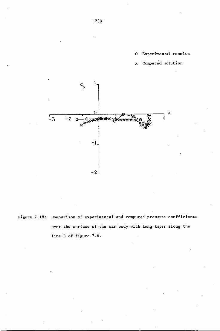
-3 -2

C P

-230-

1

-1

-2

o Experimental results

x Comput~d solution

x 4

Figure 7.18: Comparison of experimental and computed pressure coefficients

over the surface of the car body with long taper along the

line E of figure 7.6.

-1

(a)

-1

(b)

C P

-1

-2

1

-1

-2

. -231-

z 3 X102

x

o Experimental results

x Computed solution

x 4

Figure 7.19: Comparison of experimental and computed pressure coefficients

over the surface of the car body with a vertical back along

the lines (a) A; (b) A' of figure 7.6.

Ca)

Cb)

C 1 p

-1

C P

-1

-1

-2

1

-1

-2

-232-

B

B'

3 Xl0 2

C

x

4

o Experimental results

x Computed solution

C'

x

4

Figure 7.20: Comparison of experimental and computed pressure coefficients

over the surface of the car body with a vertical back along

the lines Ca) Band C; Cb) B' and C' of figure 7.6.

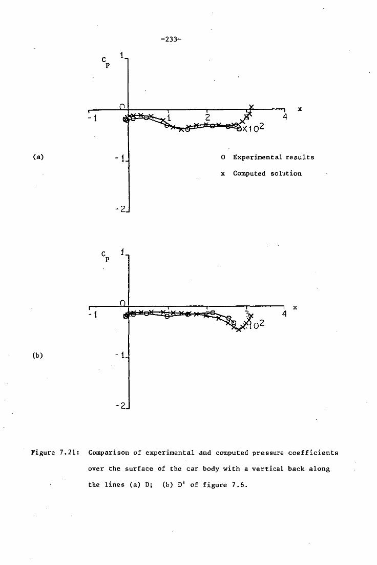
-1

(a)

- 1

(b)

C P

1

- 1

-2

C i p

- 1

-2

-233-

x

o Experimental results

x Computed solution

x 4

. 0 2

Figure 7.21: Comparison of experimental and computed pressure coefficients

over the surface of the car body with a vertical back along

the lines (a) D; (b) D' of figure 7.6.

C i p

-1

-2

-234-

o Experimental results

x Computed solution

Figure 7 .. 22: Comparison of experimental and computed pressure coefficients

over the surface of the car body with a vertical back along

the line E of figure 7.6.

-235-

SECTION"S"

CONCLUSIONS AND SUGGESTIONS FOR FURTHER WORK

A direct boundary element method for predicting the flow field

around road vehicles has been presented. The method has been compared

with the indirect boundary element method and it is concluded that the

direct method gives better results for a body with a tubular wake and

is also more forgiving when faced with poor element distribution over

the body. Furthermore, the direct method does not differ

significantly in comparison with the indirect method in respect of the

computing time required.

The"boundary integrals have been evaluated numerically by use of

a Gauss-quadrature rule over all the elements except those on which the

singu1ar~S lie. For integrals of the latter type, a modified

quadrature rule has been developed which gives better results as

compared to the Gauss-quadrature rule. Furthermore, the incorporation

of the modified quadrature rule does not add significantly to the

computing time required to set up the system matrices."

The direct method has also been compared for different types of

boundary elements and it is concluded that on the basis of accuracy

for a given computing time, the direct method with linear isoparametric

quadrilateral elements is better for the flowfield calculations in the

case of three-dimensional flow problems.

The use of the direct boundary element method gives rise to a

system of algebraic equations which is diagonally dominant and which

-236-

can therefore be solved by an iterative method of solution.

Convergence of the solution of this system of equations has been found

to be very rapid for the Gauss-Seidel iterative method which is,

therefore, more computationally efficient than, say the Gauss­

elimination method.

The boundary element method presented here has been shown to be

accurate when applied to simple body shapes for which the analytical

solutions are available for comparison. When applied to more

complicated body shapes, such as road vehicles, the results obtained

with the present method are in good agreement with. the experimental

results over most of the body surface, where the real flow remains

attached. Over the rear portion of the vehicle, where the boundary

layer rapidly thickens and separates. to form the wake, the theoretical

and experimental results differ more markedly. It has been shown that

the theoretical results in this area change significantly in response

to small changes in the initial shape of the wake and they will also

vary with the precise positioning of the separation of the wake.

Thus the complete analysis of the boundary layer growth and the position

of boundary layer separation is required to remove this discrepancy

between the computed and the experimental results. The most urgent

need for further work is thus the implementation of a boundary layer

analysis scheme. Such a scheme would require repeated use of the

potential flow analysis scheme developed in this thesis, which therefore

needs to be as efficient as possible.

As has been mentioned previously in section 5, about 90 to 95

percent of the total computing time for the current method is used on

setting up the matrices of influence coefficients. These matrices

need only be created once for a full solution .scheme including boundary

-237-

layer iteration, but even so the most significant future gain in

computational efficiency must come from effort in this area. All the

results produced in this thesis have been obtained using an 'optimize'

option at compile time, which significantly reduces the run time of

the program. Other than this, no great attention has been paid to the

efficiency of the algorithm which produces the influence coefficients.

Thus significant gain may be possible in this area, particularly by

using simpler approximations to integrals over elements at large

distances from the fixed point.

For all the work presented in this thesis the onset flow has been

taken to be a uniform stream in the direction of the x-axis, i.e.

parallel to the body. However, this restriction is not necessary and

the present method can be applied with an onset flow in any desired

direction. In particular, vehicle motion in a cross-wind could be

analysed, but some difficulty would be experienced in deciding upon

the line of wake separation in the absence of a complete boundary

layer analysis.

Furthermore all the results presented in this thesis have been for

situations where there is no net normal velocity at the body surface.

The direct method can be applied with equal ease to situations with any

chosen normal velocity, thus the modelling of boundary layer thickness

via surface transpiration or the modelling of inflow and outflow at

the radiator grille and ventilation grilles could easily be considered

in future developments.

-238-

REFERENCES

(1) Hucho, W.H. (1983): "Designing Cars for low drag - state of

the art and future potential", Int.J. of Vehicle Design,

Technological Advances in Vehicle Design Series.SP3, Impact of

Aerodynamics on Vehicle Design, pp 1-8.

(2) Landahl, M.T.: "Numerical Modelling of blunt-body flows -

Problems and Prospects", Proceedings of the G.M. - Symposium,

Aerodynamic Drag Mechanismrof Bluff - Bodies and Road Vehicles,

Plenum Press, 1978.

(3) Hirt, C.W. and Ramshaw, W.H.: "Prospects for numerical

simulation of bluff body aerodynamics", Proceedings of the G.M.­

Symposium, Aerodynamic Drag Mechanisms of Bluff - Bodies and

Road Vehicles, Plenum Press, 1978.

(4) Markatos, N.G. (1983): "The theoretical prediction of external

aerodynamics of road vehicles", Int. J of Vehicle Design,

Technological Advances in Vehicle Design Series, SP3, Impact

of Aerodynamics on Vehicle Design, pp 387-400.

(5) Demuren, A.O. and Rodi, W.: "Calculation of three-dimensional

turbulent flow around car bodies", Proceedings of the International

Symposium on 'Vehicle Aerodynamics', Volkswagenwerk AG,

December, 1982.

-239-

(6) Ecer, A.: "The application -of Finite element methods for the

prediction of flow around road vehicles", Proceedings of the

International Symposium on 'Vehicle Aerodynamics',

Volkswagenwerk AG, December, 1982.

(7) Hess, J.L. and Smith, A.M.O.: "Calculation of non-lifting

potential flow about arbitrary three-dimensional bodies",

lkDonnel Douglas Report No. E.S. 40622 1962.

(8) Hess, J.L. and Smith, A.M.O.: "Calculation of potential flow

about arbitrary bodies", Progress in Aeronautical Sciences,

Vol. 8, pp 1-158, Pergamon Press 1967.

(9) Hess, J. L. and Martin, R. P. Jr.: "Improved Solution for

potential flow about arbitrary axisymmetric bodies by the use

of a higher-order surface source method", Computer Methods in

Applied Mechanics and Engineering, VS n3 May 1975 P297-308.

(10) Hess, J .L.: "Higher order numerical solutions of the int'egral

equation for the two-dimensional Neumann probleui", Computer­

Methods in Applied Mechanics and Engineering, Vol. 2, 1973

pp 1-15.

(11) Morino, L.: Chen, Lee-Tzong and Suciu, E.O.: "A Steady and

oscillatory subsonic and supersonic aerodynamics around complex

configurations", -AIAA Journal,- Vol. 13, No 3 March 1975,

pp 368-374.

-240-

(12) Maskew, B.: "Prediction of subsonic aerodynamic characteristics:

A Case for low-order panel methods", J. Aircraft Vol. 19,

No. 2 Feb 1982.

(13) Stafford, L.G.: "An improved numerical method for the

calculation of the·flow-fie1d around a motor vehicle", Paper 11,

Advances in Road Vehicle Aerodynamics, Ed. H.S. Stephen's, BHRA

Fluid Engineering, Cranfie1d, 1974.

(14) Ahmed, S.R. and Hucho, W.H.: "The calculation of the flow field

past a van with the aid of a panel method", SAE Paper No. 770390,

1977.

(15) Berta, C; Tacca, T. and Zucchelli, A.: "Aerodynamic Study on

vehicle shape with the "Panel method: An effort to calculate the

influence of shape characterestics on aerodynamic performance",

SAE Paper No. 801401 1980.

(16) Stafford, L.G. (1983): "A higher order boundary integral

equation technique for the computation of vehicle flow fields" ,

Int. J. of Vehicle Design, Technological Advances in Vehicle

Design Series, SP3, Impact of aerodynamics on Vehicle Design,

pp 401-428

(17) Djojodihardjo, H.: "Development of aerodynamic computation

routine for road vehicles using panel method", Second

International Pacific Conference on Automotive Engineering, 1983,

SAE Publication P-139.

-241-

(18) Losito, V.; de Nico1a, C.; Albertoni, S. and Berta, C. (1983):

"Numerical solutions of potential and viscous flow around road

vehicles", Int. J. of Vehicle Design, Technological Advances in

Vehicle Design Series, SP3, Impact of Aerodynamics on Vehicle

Design, pp 429-440.

(19) Losito, V. and de Nicola, C. (1983): "An improved method of

computing the wake effects on aerodynamic characteristics of

road vehicles", Int. J. of Vehicle Design, Technological

Advances in Vehicle Design Series, SP3, Impact of Aerodynamics

on Vehicle Design, pp 441-450.

(20) Chomenton, F. (1983): "Calculation of three-dimensional

separated flow around road vehicles", Int. J. of Vehicle Design,

Technological Advances in Vehicle Design Series, SP3, Impact of

Aerodynamicson Vehicle Design, pp 374-386.

(21) Hirsche1,oE.H. and Bretthauer, N. and Rohe, H.: "Theoretical

and experimental boundary-layer Studies on car bodies",

Proceedings of the International Symposium on 'Vehicle

Aerodynamics', Volkswagenwerk AG, December 1982.

(22) Sunnna, J. M. and Maskew, B.: "Predicting automobile

aerodynamic characteristios using an iterative viscous/potential

flow technique", SAE Technical Paper 830303.

(23) Lamb, H.: "Hydrodynamics" 6th Edition, Cambridge University

Press (1932).

-242-

(24) Milne-Thomson, L.M.: "Theoretical Hydrodynamics", 5th Edition,

London Macmillan & Co Ltd 1968.

(25) Kellogg, O.D.: "Foundations of Potential Theory", Frederick

Ungar Publishing Company, (1929).

(26) Brebbia, C.A. and Walker, S.: "Boundary Element Techniques in

Engineering", Newnes-Butterworths (1980).

(27) Huebner, K.H.: "The Finite Element Method for Engineers",

John-Wiley, (1975).

(28) Zienkiewicz, O. C.: "The Finite Element Method", McGraw-Hill,

London, (1977).

(29) Brebbia, C.A.: "The Boundary Element Methods for Engineers",

Pentech Press (1978).

(30) Stroud, A.H. and Secrest, D.: "Gaussian Quadrature Formulae",

Prentice Hall, New York, (1966).

(31) Nobel, B. and Daniel, J.W.: "Applied Linear Algebra", Second

Edition, Prentice-Hall (1977).

(32) Vallentine, H.R.: "Applied Hydrodynamics", Butterworth & Co

(Publishers) Limited, S.l. Edition (1969).

-243-

(33) Peat, K. S. : "Potential flow about two spheres", Internal Report

1985/38, Department of Engineering Mathematics, Loughborough

University of Technology.

(34) Groh, G.G.: Comment on "Prediction of subsonic aerodynamic

characteristics: A case for low-order panel method",

J. Aircraft Vol. 22, No. 1 (1985).

(35) Cristescue, M. and Loubignac, G: "Gaussian quadrature formulas

with singularities in it over triangles and quadrangles",

Recent Advances in Boundary Element Methods, Edited by

Brebbia, C.A., Pentech Press London (1978).

' .

. '

\