Embed Size (px)
Citation preview
mathematics of computationvolume 55, number 192october 1990, pages 451-472
BOUNDARY INTEGRAL EQUATION METHODSFOR SOLVING LAPLACE'S EQUATION
WITH NONLINEAR BOUNDARY CONDITIONS:
THE SMOOTH BOUNDARY CASE
KENDALL E. ATKINSON AND GRAEME CHANDLER
Abstract. A nonlinear boundary value problem for Laplace's equation is
solved numerically by using a reformulation as a nonlinear boundary integral
equation. Two numerical methods are proposed and analyzed for discretizing
the integral equation, both using product integration to approximate the singu-
lar integrals in the equation. The first method uses the product Simpson's rule,
and the second is based on trigonometric interpolation. Iterative methods (in-
cluding two-grid methods) for solving the resulting nonlinear systems are also
discussed extensively. Numerical examples are included.
1. Introduction
Consider solving the nonlinear boundary value problem
(1.1) Au(P) = 0, PgD,
(1.2) z^p. = .g<ptUlp)) + fip)t PGY = dD.
We study the numerical solution of a nonlinear boundary integral equation
reformulation of this problem, a reformulation that has been studied recently
in Ruotsalainen and Wendland [8]. In (1.1), we assume D is a bounded, simply
connected open region in K with a smooth boundary Y, and we seek a solution
ugC (D) n CX(D). Our numerical methods generalize to other problems, for
example exterior problems, but these are not considered here. Also in (1.2), np
denotes the exterior unit normal to T at P, and the function / is assumed
given and continuous on Y. The function g(P,v) is assumed to be continuous
for (P, v) G Y x E, although this can be relaxed. Further assumptions on g
are given later.
Received June 29, 1989.1980 Mathematics Subject Classification (1985 Revision). Primary 65R20; Secondary 31A10,
45L10, 65J15, 65N99.This paper was written while the first author was a Visiting Professor in the Department of
Mathematics of the University of Queensland, Brisbane, Australia. The first author was supported
by the University of New South Wales ARC program grant Numerical analysis for integrals, integral
equations, and boundary value problems.
© 1990 American Mathematical Society0025-5718/90 $1.00+ $.25 per page
451
License or copyright restrictions may apply to redistribution; see https://www.ams.org/journal-terms-of-use
452 K. E. ATKINSON AND GRAEME CHANDLER
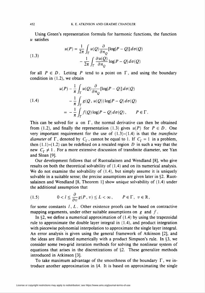
Using Green's representation formula for harmonic functions, the function
u satisfies
(1.3)
u(P) = ¿ Jr u(Q)-^-[log\P - Q\]da(Q)
¡d^log\P-Q\da(Q)Jr on02tt~
for all P G D. Letting P tend to a point on Y, and using the boundary
condition in (1.2), we obtain
u(P) - i f u(Q)-£-[log\P - Q\]da(Q)71 'r anQ
(1.4) -I f g(Q,u(Q))log\P-Q\da(Q)
= -i [ f(Q)log\P-Q\do(Q), PgY.n Jr
This can be solved for « on T, the normal derivative can then be obtained
from (1.2), and finally the representation (1.3) gives u(P) for P G D. One
very important requirement for the use of (1.3)—(1.4) is that the transfinite
diameter of Y, denoted by Cr, cannot be equal to 1. If Cr = 1 in a problem,
then (1.1 )—( 1.2) can be redefined on a rescaled region D in such a way that the
new Cr ^ 1. For a more extensive discussion of transfinite diameter, see Yan
and Sloan [9].
Our development follows that of Ruotsalainen and Wendland [8], who give
results on both the theoretical solvability of (1.4) and on its numerical analysis.
We do not examine the solvability of (1.4), but simply assume it is uniquely
solvable in a suitable sense; the precise assumptions are given later in §2. Ruot-
salainen and Wendland [8, Theorem 1] show unique solvability of (1.4) under
the additional assumption that
(1.5) 0</< — g(P, v) <L<cx>, PgY,vgR,
for some constants I, L. Other existence proofs can be based on contractive
mapping arguments, under other suitable assumptions on g and /.
In §2, we define a numerical approximation of (1.4) by using the trapezoidal
rule to approximate the double layer integral in (1.4), and product integration
with piecewise polynomial interpolation to approximate the single layer integral.
An error analysis is given using the general framework of Atkinson [2], and
the ideas are illustrated numerically with a product Simpson's rule. In §3, we
consider some two-grid iteration methods for solving the nonlinear system of
equations that arises in the discretizations of §2. These generalize methods
introduced in Atkinson [3].
To take maximum advantage of the smoothness of the boundary Y, we in-
troduce another approximation in §4. It is based on approximating the single
License or copyright restrictions may apply to redistribution; see https://www.ams.org/journal-terms-of-use
BOUNDARY INTEGRAL EQUATION METHODS 453
layer integral operator in (1.4) by product integration with trigonometric inter-
polation. The error analysis is slightly more difficult than that for the piecewise
polynomial product integration of §2, but the convergence is much faster, as is
illustrated in the numerical examples.
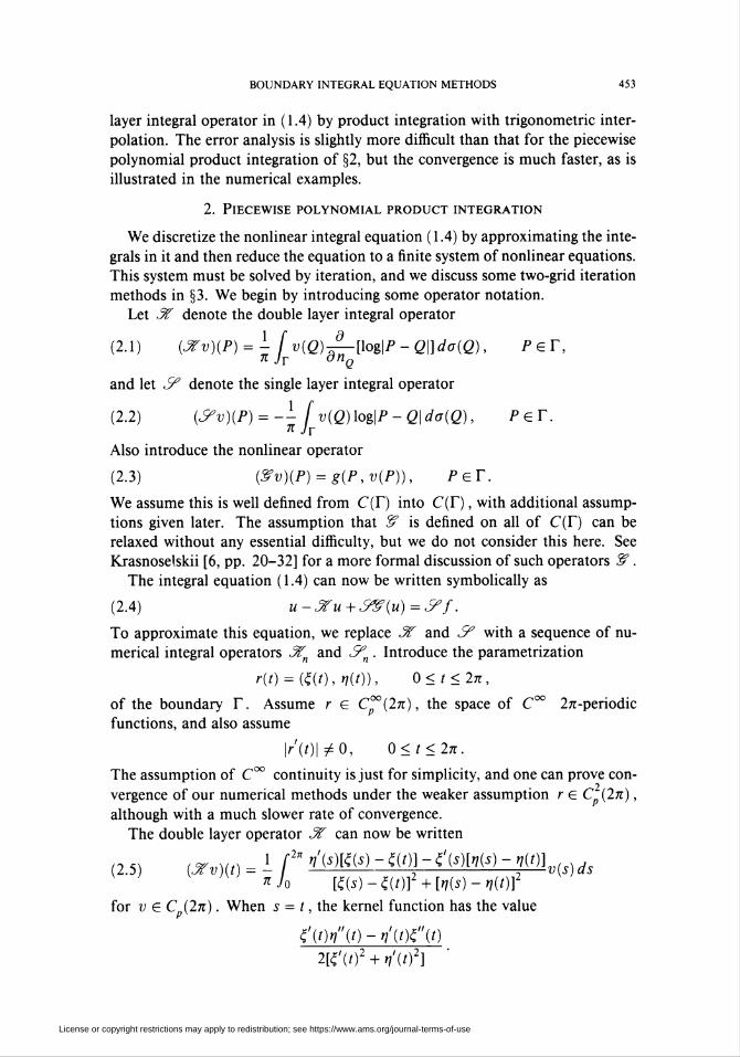
2. Piecewise polynomial product integration
We discretize the nonlinear integral equation (1.4) by approximating the inte-
grals in it and then reduce the equation to a finite system of nonlinear equations.
This system must be solved by iteration, and we discuss some two-grid iteration
methods in §3. We begin by introducing some operator notation.
Let 3Í denote the double layer integral operator
(2.1) (^v)(P)=X-[v(Q)^-[log\P-Q\]da(Q), PgY,n Jr dnQ
and let ¿9* denote the single layer integral operator
(2.2) (^v)(P) = -- [ v(Q) log\P - Q\ da(Q), PgY.n Jr
Also introduce the nonlinear operator
(2.3) (&v)(P) = g(P,v(P)), PgY.
We assume this is well defined from C(Y) into C(r), with additional assump-
tions given later. The assumption that "§ is defined on all of C(Y) can be
relaxed without any essential difficulty, but we do not consider this here. See
Krasnose'.skii [6, pp. 20-32] for a more formal discussion of such operators & .
The integral equation (1.4) can now be written symbolically as
(2.4) u-3tru+S&{u)=&'f.
To approximate this equation, we replace 3? and S? with a sequence of nu-
merical integral operators 3i„ and S?n . Introduce the parametrization
r(i) = (*(<), *(<))> 0< í < 2tt,
of the boundary Y. Assume r G C°°(2n), the space of C°° 2^-periodic
functions, and also assume
|r'(f)|/0, 0<t<2n.
The assumption of C°° continuity is just for simplicity, and one can prove con-
vergence of our numerical methods under the weaker assumption r G C (2n),
although with a much slower rate of convergence.
The double layer operator 5? can now be written
(2.5) (jr«)(o = l- F ^^-^¡-^^-fK(s)ds
for v G C (2n). When s = t, the kernel function has the value
Z'jtW'jt) - »'(()£'(t)2[c;'(t)2 + n'(t)2]
License or copyright restrictions may apply to redistribution; see https://www.ams.org/journal-terms-of-use
454 K. E. ATKINSON AND GRAEME CHANDLER
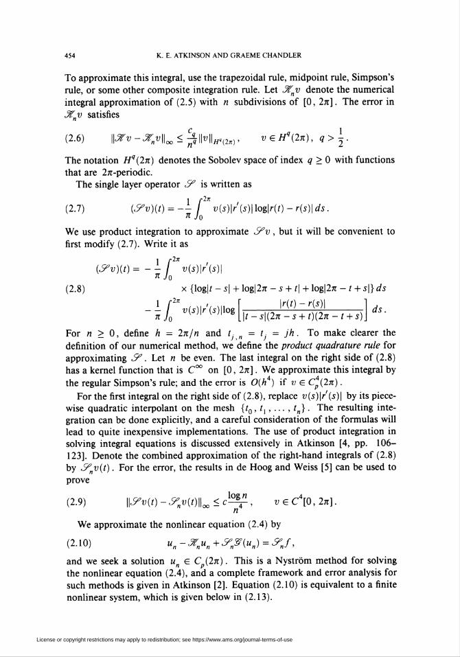
To approximate this integral, use the trapezoidal rule, midpoint rule, Simpson's
rule, or some other composite integration rule. Let 3£„v denote the numerical
integral approximation of (2.5) with n subdivisions of [0, 2k] . The error in
3?v satisfiesn
(2.6) Wv-Xnv\\x<C-±\\v\\H,{2n), vGHq(2n), q>\.
The notation H9(2n) denotes the Sobolev space of index q > 0 with functions
that are 27t-periodic.
The single layer operator 5? is written as
(2.7) (&v)(t) = ~f* v(s)\r'(s)\log\r(t) - r(s)\ ds.x Jo
We use product integration to approximate S^v , but it will be convenient to
first modify (2.7). Write it as
(S?v)(t)= -U2nv(s)\r'(s)\n Jo
(2.8) x {log|i - s| + l0g|27T - S + t\ + l0g|27T - t + s\) ds
1 f2n- \ v(s)\r (s)\logn Jo
\r(t)-r(s)\
[\t - s\(2n - s + t)(2n - t + s)\ds.
For n > 0, define h = 2n/n and t- n = t¡ = jh. To make clearer the
definition of our numerical method, we define the product quadrature rule for
approximating S". Let n be even. The last integral on the right side of (2.8)
has a kernel function that is C°° on [0, 2n]. We approximate this integral by
the regular Simpson's rule; and the error is 0(h ) if v G Cp (2n).
For the first integral on the right side of (2.8), replace v(s)\r'(s)\ by its piece-
wise quadratic interpolant on the mesh {t0, tx, ... , t„}. The resulting inte-
gration can be done explicitly, and a careful consideration of the formulas will
lead to quite inexpensive implementations. The use of product integration in
solving integral equations is discussed extensively in Atkinson [4, pp. 106—
123]. Denote the combined approximation of the right-hand integrals of (2.8)
by y„v(t). For the error, the results in de Hoog and Weiss [5] can be used to
prove
(2.9) 11^(0 -^Wlloo < ̂ , v G C4[0, 27t].
We approximate the nonlinear equation (2.4) by
(2.10) u„-Jfnu„+^n^(u„)=^J,
and we seek a solution u„ G C (2n). This is a Nyström method for solving
the nonlinear equation (2.4), and a complete framework and error analysis for
such methods is given in Atkinson [2]. Equation (2.10) is equivalent to a finite
nonlinear system, which is given below in (2.13).
License or copyright restrictions may apply to redistribution; see https://www.ams.org/journal-terms-of-use
BOUNDARY INTEGRAL EQUATION METHODS 455
Let the linear operators 3?n and ¿9'n be written as
n
(2.11) {Xnv){t) = YáwjKit,tj)v{tj), tG[0,2n],7=0
(2.12) (<9>nv)(t) = Yœjit)vitJ)< tG[0,2n].7=0
The kernel function K(t, s) is given in (2.5), and the weights {co(t)} are
obtained from the approximation of the right-hand integrals in (2.8). For (2.11 ),
we will use Simpson's rule as the quadrature method, partially to be consistent
with the earlier definition given for (2.12). Just as with the linear Nyström
method (see Atkinson [4, p. 88]), equation (2.10) is equivalent to a finite system
of equations,
n n
Un(ti)-YWjKiti'tj)Unitj) + TiC°jiti)Sitj'Unitj))
(2.13) r
7=0
The grid function that solves (2.13) is extended to a function on [0, 2n] by
means of the Nyström interpolation formula
n
unit)=YtwjK(t,tj)un(tj)
(2.14)
+ £>/')[-*('; » U„(t■•))+ f(l,)].7=0
We use this formula in the two-grid iteration method presented in §3.
The error analysis of (2.10) can be carried out within the framework of [2],
Write (2.4) and (2.10) in the shortened form
(2.15) u = &(u),
(2.16) u„=S?n(u„),
respectively. With the assumption of 2? following (2.3), the operator 5f is
compact from C(Y) into C(Y). We must also have that S? is continuous,
and thus we assume
[Al] S\ C(Y) -f C(Y) is continuous.
With this and the known properties of X and 5?, it follows that Jz? is com-
pletely continuous (compact and continuous) from C(Y) into C(Y). The as-
sumption [Al] is true if g(P, v) satisfies the Lipschitz condition
\g(P, vx) - g(P, v2)\ < c\vx - v2\x, PgY,
for some exponent Xg (0, 1] and constant c > 0.
License or copyright restrictions may apply to redistribution; see https://www.ams.org/journal-terms-of-use
456 K. E. ATKINSON AND GRAEME CHANDLER
The framework of [2] assumes that {¿zf„} satisfies the following four prop-
erties:
[HI] J? and 2Cn, n > 1, are completely continuous operators on a Banach
space 3f into itself.
[H2] {J2?} is a collectively compact family, i.e., for every bounded set B in
2f, the set [j^S?„(B) has compact closure in 2f.
[H3] For every vg%? ,
^„v —► £?v as n —► oo.
[H4] At each vgS?, {S?f\ is an equicontinuous family.
These assumptions are true for our approximations Jz? . In [HI], we let 2f =
C(Y). The complete continuity of Jz^ follows from [Al] and the compactness
of the finite-rank operators 3?n and ¿?n . For [H2], the proof of the collective
compactness of {Jz^} follows from that of {3?n} and {^„}, and the latter
are well-known results (e.g., see Atkinson [4, pp. 97, 108]). The proof of [H3]
again follows from the same result for {J^n} and {J5^}, along with the fact
that &{v) G C(Y). For [H4], use
ll-2>,) - -^Mloo < WnW IK - Moo + «I ll^(«i) - S^llo«, •The families {3?n} and {¿9^} are uniformly bounded, and then [Al] com-
pletes the proof of equicontinuity. We state the following existence theorem
for approximate solutions u„ without proof. It is a direct statement from [2,
Theorem 3].
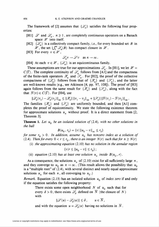
Theorem 1. Let u0 be an isolated solution of (2.4), with no other solutions in
the ball
Biuo> >"o) = 'MIK-*;lloo <r0}
for some r0 > 0. In addition, assume u0 has nonzero index as a solution of
(2.4). Then for every 0 < r < rQ, there is an integer N(r) such that for n > N(r)
(i) the approximating equation (2.10) has no solution in the annular region
{v\r< \\u0-v\\ <r0};
(ii) equation (2.10) has at least one solution u„ inside B(u0, r).
As a consequence, the solutions un of (2.10) exist for all sufficiently large 77,
and they converge to u0 as n-»oo. (This result allows the possibility that w0
is a "multiple root" of (2.4), with several distinct and nearly equal approximate
solutions u„ for each n , all converging to «0 .)
Remark. Equation (2.15) has an isolated solution u0 of index zero if and only
if the equation satisfies the following property:
There exists some open neighborhood N of u0 such that for
every S > 0, there exists J?s defined on TV (the closure of TV )
with
\\^(u)-^â(u)\\<ô, UGÑ,
and with the equation u = Jîfô(u) having no solutions in N.
License or copyright restrictions may apply to redistribution; see https://www.ams.org/journal-terms-of-use
BOUNDARY INTEGRAL EQUATION METHODS 457
Thus, a solution u0 has nonzero index if and only if the existence of solutions
to the equation is stable with respect to small perturbations of the equation. In
general, we would consider solving only those equations in which the solution
u0 possesses this type of stability.
To obtain results on the rate of convergence of un to u0, an additional
assumption is needed for the operators Jz? and Jz? :
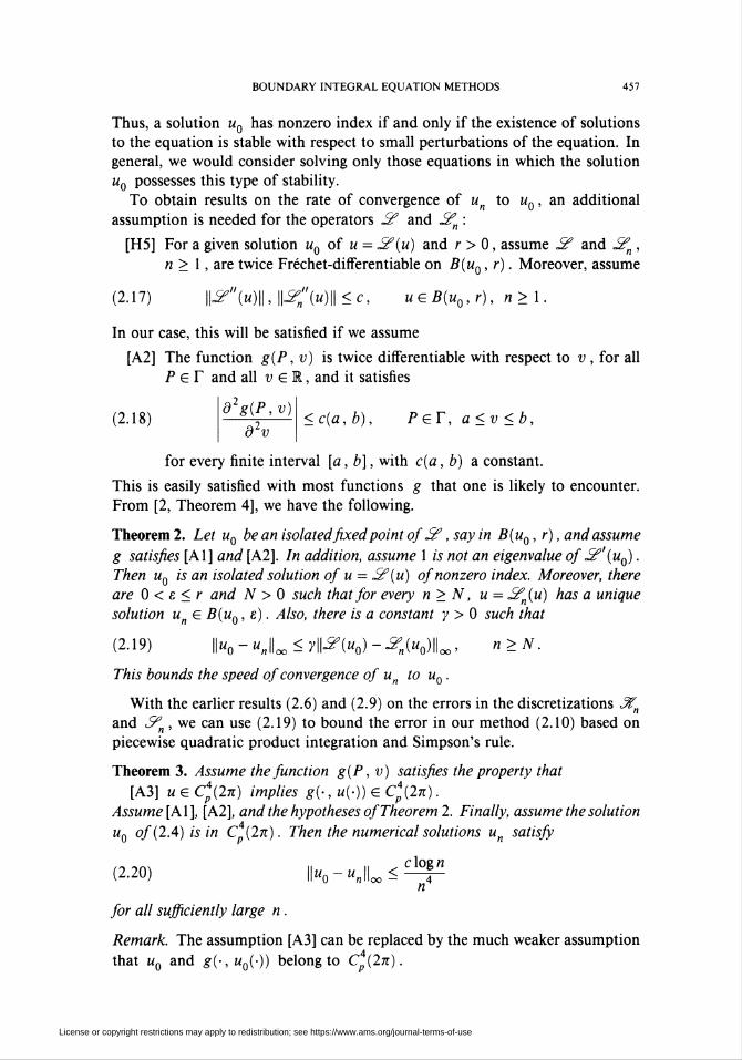
[H5] For a given solution w0 of u = S?(u) and r > 0, assume a? and Jz? ,
n > 1, are twice Frechet-differentiable on B(u0, r). Moreover, assume
(2.17) \\ä?"(u)\\,\\X'(u)\\<c, uGB(uQ,r), n>\.
In our case, this will be satisfied if we assume
[A2] The function g(P, v) is twice differentiable with respect to v , for all
PgY and all v el, and it satisfies
(2.18)d2g(P,v)
d2v<c(a,b), PgY, a <v < b,
for every finite interval [a, b], with c(a, b) a constant.
This is easily satisfied with most functions g that one is likely to encounter.
From [2, Theorem 4], we have the following.
Theorem 2. Let u0 be an isolatedfixed point of 2?, say in B(u0, r), and assume
g satisfies [Al] and [A2]. In addition, assume 1 is not an eigenvalue of'2C'(u0).
Then u0 is an isolated solution of u = ¿2?(u) of nonzero index. Moreover, there
are 0 < e < r and N > 0 such that for every n > N, u = ¿¿'„(u) has a unique
solution u„G B(u0, e). Also, there is a constant y > 0 such that
(2-19) IK - «„ll«, < yll-^K) --2>o)Hoo. « > N.
This bounds the speed of convergence of un to u0.
With the earlier results (2.6) and (2.9) on the errors in the discretizations Jf„
and Sr°n , we can use (2.19) to bound the error in our method (2.10) based on
piecewise quadratic product integration and Simpson's rule.
Theorem 3. Assume the function g(P, v) satisfies the property that
[A3] u G Cp(2n) implies g(-, «(•)) G Cp(2n).
Assume [Al], [A2], and the hypotheses of Theorem 2. Finally, assume the solution
u0 of'(2.4) is in C (2k). Then the numerical solutions u„ satisfy
<*> im ii ii , clogn(2-2°) IK - «Jo«, ̂ —f-
n
for all sufficiently large n .
Remark. The assumption [A3] can be replaced by the much weaker assumption
that u0 and g(-, uJ-)) belong to Ca(2k).
License or copyright restrictions may apply to redistribution; see https://www.ams.org/journal-terms-of-use
458 K. E. ATKINSON AND GRAEME CHANDLER
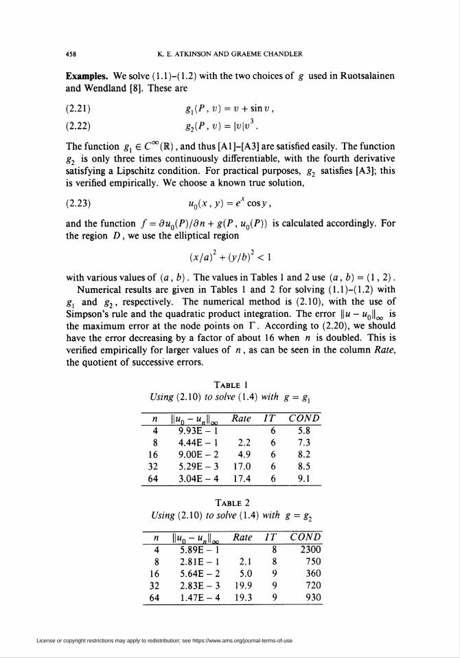
Examples. We solve ( 1.1 )-( 1.2) with the two choices of g used in Ruotsalainen
and Wendland [8]. These are
(2.21) gx(P, v) = v + sinv ,
(2.22) g2(P, v) = \v\v\
The function gx G C°°(K), and thus [A1]-[A3] are satisfied easily. The function
g2 is only three times continuously differentiable, with the fourth derivative
satisfying a Lipschitz condition. For practical purposes, g2 satisfies [A3]; this
is verified empirically. We choose a known true solution,
(2.23) u0(x, y) = excosy,
and the function / = du0(P)/dn + g(P, u0(P)) is calculated accordingly. For
the region D, we use the elliptical region
(x/a)2 + (y/bf < 1
with various values of (a, b). The values in Tables 1 and 2 use (a, b) = (1, 2).
Numerical results are given in Tables 1 and 2 for solving ( 1.1 )—( 1.2) with
g{ and g2, respectively. The numerical method is (2.10), with the use of
Simpson's rule and the quadratic product integration. The error ||w - w0IL is
the maximum error at the node points on Y. According to (2.20), we should
have the error decreasing by a factor of about 16 when n is doubled. This is
verified empirically for larger values of n , as can be seen in the column Rate,
the quotient of successive errors.
Table 1
Using (2.10) to solve (1.4) with g = gx
n IK-",, IL Rate IT COND4 9.93E-1 6 5.88 4.44E-1 2.2 6 7.3
16 9.00E-2 4.9 6 8.232 5.29E-3 17.0 6 8.5
64 3.04E-4 17.4 6 9.1
Table 2
Using (2.10) to solve (1.4) with g = g2
n IK~"JL Rate IT COND4 5.89E-1 8 23008 2.81E-1 2.1 8 750
16 5.64E-2 5.0 9 360
32 2.83E-3 19.9 9 72064 1.47E-4 19.3 9 930
License or copyright restrictions may apply to redistribution; see https://www.ams.org/journal-terms-of-use
BOUNDARY INTEGRAL EQUATION METHODS 459
The nonlinear system (2.13) was solved iteratively using Newton's method:
(2.24) un =u„ -\I-^n(un )] [u„ -¿r„{un )].
The initial guess chosen was
(2.25) uf = u0 + 1.
We iterated until the relative correction satisfied
n,.(*) f.(*-i)ii\\U — U _14(2.26) ILa—^-^°<io-14.
II" IIIl n Hoc
All norms are maximum norms over the values at the nodes on Y. The column
IT gives the lowest value of k for which (2.26) was satisfied. The column
COND gives the LINPACK condition number for the matrix associated with
I — Sf'n(vkn ) for the final iterate. Note the values of IT are essentially constant
with increasing n . This is an illustration of the mesh independence principle
discussed in Allgower et al. [1]. All of the numerical examples of this paper
were computed on an 80286/287 microcomputer.
3. Iterative solution of discretized equation
The approximating integral equation (2.10) of the preceding section can be
solved using Newton's method (2.24), as was done in the numerical examples
of the last section. This is rapidly convergent, but it is also quite costly. Each
iteration involves solving a system of order n + 1 at a cost of about 2« /3
arithmetic operations. In this section, we consider other iteration methods that
are less costly. Another source of inefficiency in constructing Tables 1 and 2
was that the nonlinear system was solved to much greater accuracy than jus-
tified by the size of ||w0 - «JL > mostly to illustrate the iteration method for
different values of n . A practical program would attempt to iterate only until
IK-i'lL was comparable to „«„-«JL-The simplest modification of Newton's method (2.24) is to fix the derivative
matrix I—^(un ) for iterates of index k > k , for some k > 0. The iteration
then becomes
(3.1) [/-^>í))]í) = -í),
(*+.)(*>(*)n n ' n
For iterates u( ' with k > k , the cost of (3.1) is 0(n ) operations per iterate,
since the LU factorization of / - 5?^(u{n J) will have already been computed.
The rate of convergence of (3.1) will only be linear, in contrast to the qua-
dratic convergence of the Newton method (2.24). The iterates satisfy
(3 2) *„ - «¡Í+1) = {/-[/-^'("¡.V'l/ -¿ÍG01H«, - «¡Î}]
+ 0(\\u„-u(nk)\\2).
License or copyright restrictions may apply to redistribution; see https://www.ams.org/journal-terms-of-use
460 K. E. ATKINSON AND GRAEME CHANDLER
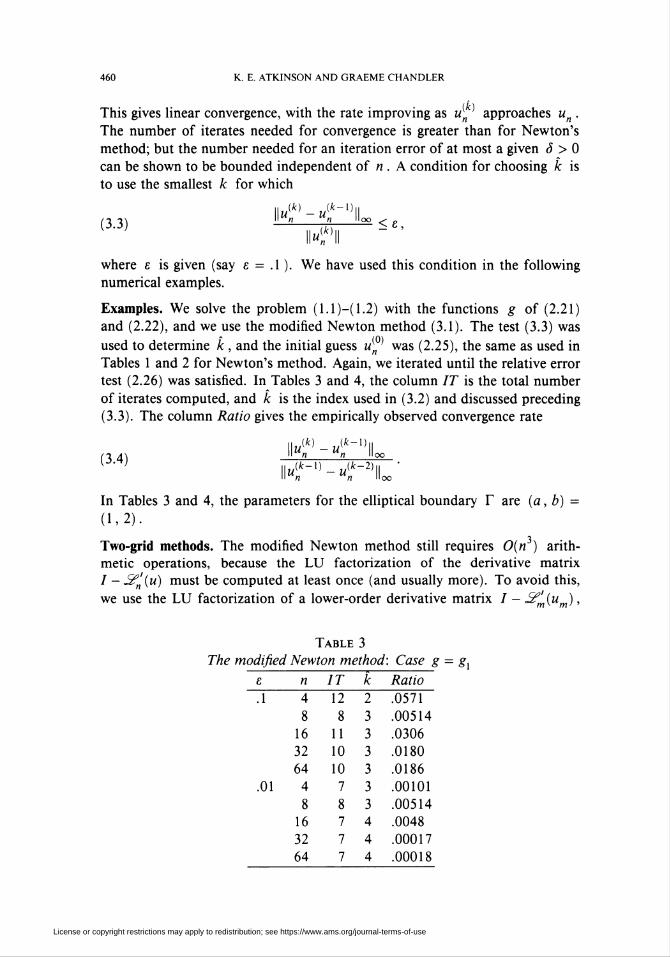
(k)This gives linear convergence, with the rate improving as u„ approaches u„ .
The number of iterates needed for convergence is greater than for Newton's
method; but the number needed for an iteration error of at most a given Ô > 0
can be shown to be bounded independent of n . A condition for choosing k is
to use the smallest k for which
\\u{k]-u{k-X)\\(3.3) " " " "°°<e,
Wun I
where e is given (say e = A). We have used this condition in the following
numerical examples.
Examples. We solve the problem (1.1 )—( 1.2) with the functions g of (2.21)
and (2.22), and we use the modified Newton method (3.1). The test (3.3) was
used to determine k , and the initial guess un was (2.25), the same as used in
Tables 1 and 2 for Newton's method. Again, we iterated until the relative error
test (2.26) was satisfied. In Tables 3 and 4, the column IT is the total number
of iterates computed, and k is the index used in (3.2) and discussed preceding
(3.3). The column Ratio gives the empirically observed convergence rate
ii (k) (¿-On\\u — u \\(3 4) JL-H_i-[!oo_
IIív^-"-^-2'!! '»un un Hoc
In Tables 3 and 4, the parameters for the elliptical boundary Y are (a, b) =
(1,2).
Two-grid methods. The modified Newton method still requires 0(n3) arith-
metic operations, because the LU factorization of the derivative matrix
/ - ^f'(u) must be computed at least once (and usually more). To avoid this,
we use the LU factorization of a lower-order derivative matrix / - &'(u ),
Table 3
The modified Newton method: Case g = gx
e n IT k Ratio
.1 4 12 2 .0571
8 8 3 .0051416 11 3 .030632 10 3 .018064 10 3 .0186
.01 4 7 3 .00101
8 8 3 .0051416 7 4 .0048
32 7 4 .0001764 7 4 .00018
License or copyright restrictions may apply to redistribution; see https://www.ams.org/journal-terms-of-use
BOUNDARY INTEGRAL EQUATION METHODS 461
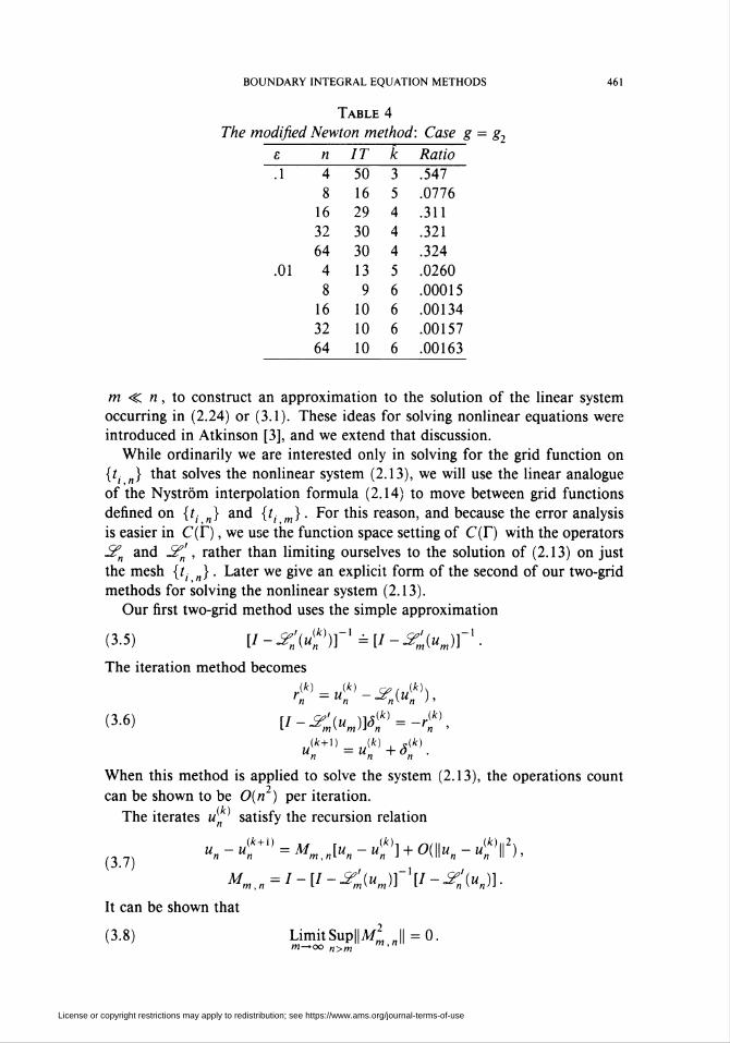
Table 4
The modified Newton method: Case g = g2
e n IT k Ratio~1 4 50 3 ^47
8 16 5 .077616 29 4 .311
32 30 4 .32164 30 4 .324
.01 4 13 5 .02608 9 6 .00015
16 10 6 .00134
32 10 6 .0015764 10 6 .00163
m < n, to construct an approximation to the solution of the linear system
occurring in (2.24) or (3.1). These ideas for solving nonlinear equations were
introduced in Atkinson [3], and we extend that discussion.
While ordinarily we are interested only in solving for the grid function on
{tj „} that solves the nonlinear system (2.13), we will use the linear analogue
of the Nyström interpolation formula (2.14) to move between grid functions
defined on {ti „} and {/• m} . For this reason, and because the error analysis
is easier in C(Y), we use the function space setting of C(Y) with the operators
2f„ and JSf', rather than limiting ourselves to the solution of (2.13) on just
the mesh {/; „}. Later we give an explicit form of the second of our two-grid
methods for solving the nonlinear system (2.13).
Our first two-grid method uses the simple approximation
(3.5) [I -J?'(u{?)fl =[I -J^iujf1.
The iteration method becomes
Jk+l) Jk),Ak)Un =Un +ôn ■
When this method is applied to solve the system (2.13), the operations count
can be shown to be 0(n2) per iteration.
The iterates u[ J satisfy the recursion relationn
(37) u„-u{k„+X) = Mmn[un-u[kn)] + 0(\\un-u{y),
Mmi„ = I-[I-^ium)fl[I-^'iun)].
It can be shown that
(3.8) UmhSup||<J = 0.m—»oo „>m
License or copyright restrictions may apply to redistribution; see https://www.ams.org/journal-terms-of-use
462 K. E. ATKINSON AND GRAEME CHANDLER
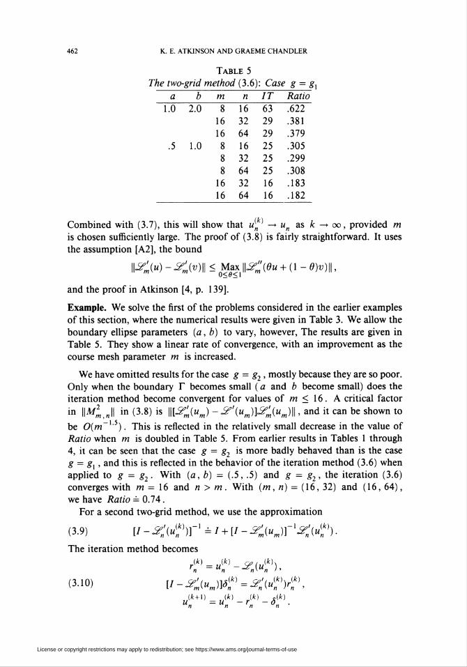
Table 5
The two-grid method (3.6): Case g = gx
a b m n IT Ratio~TÖ IÖ 8 Ï6 63 Ü22-
16 32 29 .38116 64 29 .379
.5 1.0 8 16 25 .3058 32 25 .2998 64 25 .308
16 32 16 .183
_16 64 16 .182
Combined with (3.7), this will show that u[ ] -* un as k —> oo, provided m
is chosen sufficiently large. The proof of (3.8) is fairly straightforward. It uses
the assumption [A2], the bound
ii^>)-^>)II<mm||^;'(ö«+(i-ö)«)ii,US^S 1
and the proof in Atkinson [4, p. 139].
Example. We solve the first of the problems considered in the earlier examples
of this section, where the numerical results were given in Table 3. We allow the
boundary ellipse parameters (a, b) to vary, however, The results are given in
Table 5. They show a linear rate of convergence, with an improvement as the
course mesh parameter m is increased.
We have omitted results for the case g = g2, mostly because they are so poor.
Only when the boundary Y becomes small ( a and b become small) does the
iteration method become convergent for values of m < 16. A critical factor
in \\M2m„\\ in (3.8) is ||[-2>J -^'(MJL2>J||, and it can be shown to
be 0(m~ ' ). This is reflected in the relatively small decrease in the value of
Ratio when m is doubled in Table 5. From earlier results in Tables 1 through
4, it can be seen that the case g = g2 is more badly behaved than is the case
g = gx , and this is reflected in the behavior of the iteration method (3.6) when
applied to g = g2. With (a, b) = (.5, .5) and g = g2, the iteration (3.6)
converges with m = 16 and n > m. With (m, n) = (16, 32) and (16, 64),
we have Ratio = 0.74.
For a second two-grid method, we use the approximation
(3.9) [/ - &H{uf)\-X = / + [/- K(um)]-X5f'(u{„k)).
The iteration method becomes
(3-10) v-^>Mk)=^:i«{nkv:
n n n n
License or copyright restrictions may apply to redistribution; see https://www.ams.org/journal-terms-of-use
BOUNDARY INTEGRAL EQUATION METHODS 463
The approximation in (3.9) comes from the theory of collectively compact oper-
ator approximations for linear operators; for example, see Atkinson [4, p. 94].
For the development of the iteration method (3.10) for linear operators, see
Atkinson [4, p. 142] or Atkinson [3].
The iterates u(„ ) satisfy the recursion relation
(3H) un-u[k^ = MmJun-u^] + 0(\\u„-u[kY),
Mm,n = V-Ki»jrl[^>n)-^>J]3'>n)-
It can be shown that
(3.12) LimitSupp/w J = 0.m—Kx> n>m '
The proof is fairly straightforward, just as for (3.8), and we omit it. From
(3.12), it follows easily that
(3.13) ii"„-«ri,ii<(ii^,ji+^)ii"„-i)iiwith e„ —> 0 as n -* oo. It can be shown that
(3.14) \\MmJ = 0(m-1-5).
The proof is much the same as for (4.12) in §4, and thus we omit it here.
Examples. We repeat the cases used in the preceding example, but now using the
two-grid method (3.10). The results are given in Table 6, and again they show
a linear rate of convergence. [The value of Ratio for the case (a, b) = (1, 2)
and m — 8 oscillated between two values, and the geometric mean of these
values is given in the table.] Considering the results of Tables 5 and 6, the two-
grid method (3.10) is superior to the two-grid method (3.6) when the rates of
linear convergence are compared. This has been observed in general, and some
theoretical support can be given for it.
We also solved the integral equation (2.4) with g = g2; and as was true
with (3.6), the results were much poorer than those in g = gx . There was no
Table 6
The two-grid method (3.10): Case g = gx
a b m n IT Ratio~TÖ 2X) 8 16 47 .50*
16 32 17 .18616 64 17 .178
0.5 1.0 8 16 15 .1328 32 15 .1248 64 15 .128
16 32 9 .04516 64 9 .042
License or copyright restrictions may apply to redistribution; see https://www.ams.org/journal-terms-of-use
464 K. E. ATKINSON AND GRAEME CHANDLER
convergence for (a, b) = (1, 2) or (.5, 1), with m < 16. For (a, b) = (.5, .5)
and g = g2, the iteration (3.10) converges for m = 16 and n > m. With
(n, m) = (16, 32) and (16, 64), we have Ratio = .795 and .754, respectively.
This is slightly worse than the analogous results for method (3.6), but it is
expected that the method (3.10) will be superior to (3.6) for larger values of
m.
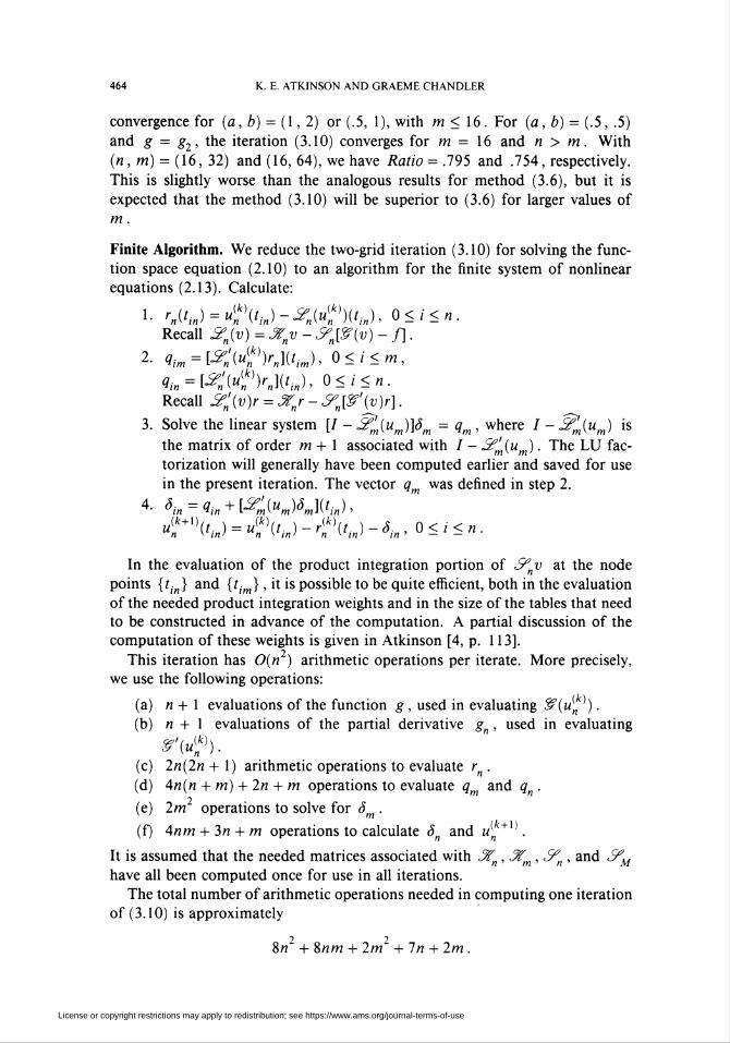
Finite Algorithm. We reduce the two-grid iteration (3.10) for solving the func-
tion space equation (2.10) to an algorithm for the finite system of nonlinear
equations (2.13). Calculate:
1- rn(tm) = u(k)(tin)-5fn(u(k))(tin), 0<i<n.
Recall &H(v)=3rttv-fn[S?(v)-f].
2- ^ = [^>!>J(0> 0<i<m,íi^^í«?1)«. 0<i<n.
Recall -?„>)/" = 3tnr - &„[&\v)r].
3. Solve the linear system [/ - 2'm(um)]àm = qm , where / - 5?m(um) is
the matrix of order m + 1 associated with / - -2^(«m). The LU fac-
torization will generally have been computed earlier and saved for use
in the present iteration. The vector qm was defined in step 2.
<k+l)iU = u[k)(U-r{nk\ti„)-S,n,0<l<n.
In the evaluation of the product integration portion of ^ti at the node
points {tjn} and {tim} , it is possible to be quite efficient, both in the evaluation
of the needed product integration weights and in the size of the tables that need
to be constructed in advance of the computation. A partial discussion of the
computation of these weights is given in Atkinson [4, p. 113].
This iteration has 0(n2) arithmetic operations per iterate. More precisely,
we use the following operations:
(a) n + 1 evaluations of the function g, used in evaluating &(u[ ').
(b) n + I evaluations of the partial derivative g„, used in evaluating
$\u(k)).
(c) 2n(2n + 1) arithmetic operations to evaluate r„.
(d) 4n(n + m) + 2n + m operations to evaluate qm and q„.
(e) 2m operations to solve for Sm .
(f) 4nm + 3n + m operations to calculate S„ and u[ +1).
It is assumed that the needed matrices associated with 3?„ , Xm , ¿9pn , and <9*M
have all been computed once for use in all iterations.
The total number of arithmetic operations needed in computing one iteration
of (3.10) is approximately
2 28« +%nm + 2m +ln + 2m.
License or copyright restrictions may apply to redistribution; see https://www.ams.org/journal-terms-of-use
BOUNDARY INTEGRAL EQUATION METHODS 465
For comparison, the analogous operations count for the two-grid method (3.6)
is
2 24« +Snm + 2m +5n + 2m.
Since the term n will dominate the remaining terms in these operation counts
for n » m , we have that the two-grid method (3.10) is about twice as expensive
per iterate as the two-grid method (3.6). Combining this with the generally
faster convergence of (3.10), the two methods seem to be roughly comparable in
computation time. Nonetheless, we have a slight preference for method (3.10),
mainly because of the convergence behavior. With nonlinear integral equations
other than those considered here, the first method (3.6) has been less regular in
its convergence, with the values of Ratio for (3.6) varying widely as the iteration
converged; see the discussion of method (3.6) for linear equations in Atkinson
[4, pp. 159-161]. But for the present work, the convergence behavior of method
(3.6) was very regular, equal to that seen with method (3.10), in contrast with
earlier work on other nonlinear integral equations. Thus there does not seem
to be any clear reason to prefer either of these two-grid methods over the other
one.
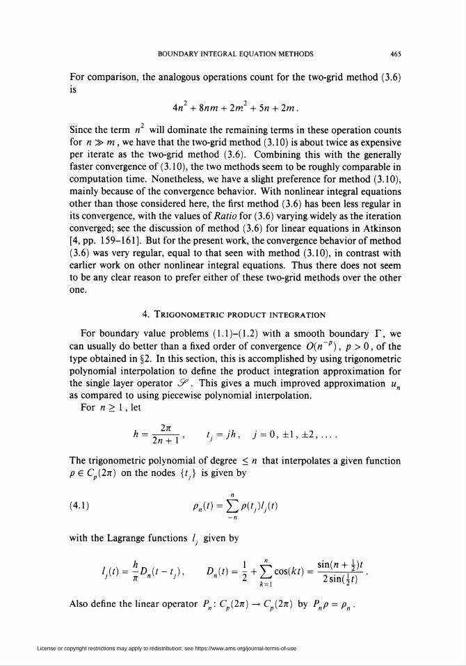
4. Trigonometric product integration
For boundary value problems (1.1 )—( 1.2) with a smooth boundary Y, we
can usually do better than a fixed order of convergence 0(n~p), p > 0, of the
type obtained in §2. In this section, this is accomplished by using trigonometric
polynomial interpolation to define the product integration approximation for
the single layer operator 5?. This gives a much improved approximation u„
as compared to using piecewise polynomial interpolation.
For n > 1, let
h = . 2n , , t,=jh, j = 0, ±1,±2, ... .2« + 1 j J > J
The trigonometric polynomial of degree < n that interpolates a given function
p G Cp(2k) on the nodes {t } is given by
(4.1) Pnit) = J2Pitj)ljit)-n
with the Lagrange functions / given by
k=\ v¿ '
Also define the linear operator P„ : Cp(2k) —> Cp(2k) by P„p = p„ .
License or copyright restrictions may apply to redistribution; see https://www.ams.org/journal-terms-of-use
466 K. E. ATKINSON AND GRAEME CHANDLER
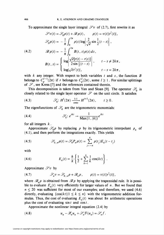
(4.2)
To approximate the single layer integral S"v of (2.7), first rewrite it as
S?v(t) = ^0p(t) + ¿gp(t), p(t) = v(t)\r'(t)\,
<9>0p(t)= -X-fK p(s)logn Jo
1 fln¿gp(t)= -- / B(t,s)p(s)ds,
*■ Jo
2 I,Te™-2(t-s)
B(t,s)={log
y/ë[r{t) ~ r(s)]
2 sin j (t - s)t- s± 2kK,
\lag\y/ër(t)\, t-s = 2kn,
with k any integer. With respect to both variables / and 5, the function B
belongs to C ~ (2k) if r belongs to Cp(2k) , some / > 1. For similar splittings
of S?, see Kress [7] and the references contained therein.
This decomposition is taken from Yan and Sloan [9]. The operator <9*Q is
closely related to the single layer operator J/7 on the unit circle. It satisfies
(4.3) ¿?í:H,(2k)-^^H,+ x(2k), t>0.
The eigenfunctions of ¿K are the trigonometric monomials:
¿7Q:eiki 1 ikt
(4'4) ~°"^ ' Max{l, |Jfe|}'
for all integers k .
Approximate S^p by replacing p by its trigonometric interpolant p„ of
(4.1), and then perform the integrations exactly. This yields
(4.5) «^0,^(0=^0^(0= E Pitj)E„it-tj)
with
(4.6) *■('> = £{£ +¿¿c«<*r)}
9„p, p(t) = v(t)\r(t)\,
Approximate S?v by
(4.7) ^„v=^np + .
where 38„p is obtained from 3§p by applying the trapezoidal rule. It is possi-
ble to evaluate £„(0 very efficiently for larger values of n . But we found that
n < 20 was sufficient for most of our examples; and therefore, we used (4.6)
directly, evaluating {cos(Ari)|l < k < n) with the trigonometric addition for-
mulas. Thus, the cost of evaluating E„(t) was about 8« arithmetic operations
plus the cost of evaluating sin / and cos t.
Approximate the nonlinear integral equation (2.4) by
(4.8) ",-■*>,+-WO = •*;/•
License or copyright restrictions may apply to redistribution; see https://www.ams.org/journal-terms-of-use
BOUNDARY INTEGRAL EQUATION METHODS 467
The trapezoidal rule applied to 3iu is used to define the numerical integral op-
erator 3if„ . As before in §2, this approximating equation is a Nyström method,
and the solving of (4.8) reduces to solving a finite system of nonlinear equations
of order 2« + 1.
The error analysis of (4.8) is similar to that used in Theorem 1, but it re-
quires some significant changes. With (4.8), we cannot prove {¿9^} is a col-
lectively compact and pointwise convergent family of operators from C (2k)
into C (2k) ; and therefore, we cannot simply invoke the results from [2] in the
manner done in Theorem 1. Instead, we construct another proof, for our situa-
tion, of the major result [2, Theorem 2]. Then we can use the subsequent results
in [2], constructing an error analysis for (4.8) in analogy with that given earlier
in Theorems 1-3 for the product quadratic method (2.10). We begin with the
following lemma on trigonometric interpolation. It can be proven using a fairly
standard manipulation of the Fourier series representation of the function p.
Lemma 4. Let p G H'(2k) with t > \; let s < t. Then the trigonometric
interpolation polynomial P„p of (4.1) satisfies
cs\\Pl(4-9) \\P-P„P\\S< J-s
n
with cs a constant and || • ||( denoting the norm in H'(2k) .
Using this lemma, we can prove a number of error bounds involving the
approximating single layer ^ „ .
Lemma 5. Let p G H'(2k) with t > \ ; let s < t + 1. Then
(4-10) Pto-^uPM $êk-
Proof. Use (4.3) to obtain
W^OP - ^0,nPl = W - PJPWs < ira IK' - Pn)P\\s-l ■
Then invoke Lemma 4 to complete the proof. G
Lemma 6. For any e > 0,
(4.11) IK^o-^o,J^oll<'n1-5-
c loe m(4-12) \\i^o-^o,n)<KJ<^Y&>
where the operators ¿9^ and ¿9^ „ are regarded as operators from C (2k) into
Cp(2k). The constant ce depends only on e.
Proof. We show only (4.12), the more difficult of the two inequalities. The
proof of (4.11) is similar. For p g Cp(2k) c H°(2k) , we have S^p g Hx(2k) .
License or copyright restrictions may apply to redistribution; see https://www.ams.org/journal-terms-of-use
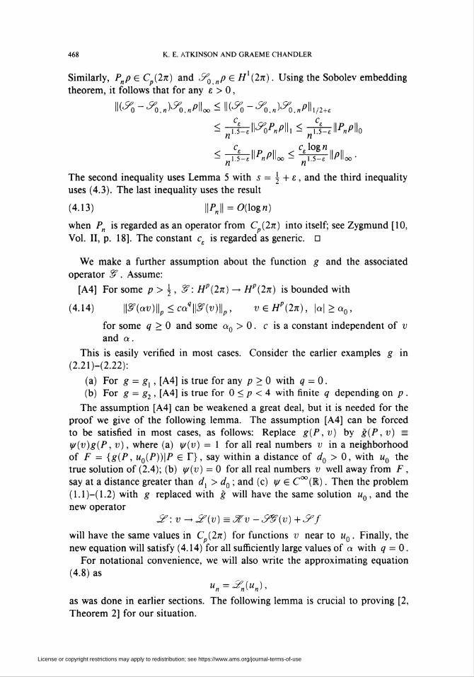
468 K. E. ATKINSON AND GRAEME CHANDLER
Similarly, Pnp g Cp(2k) and S^ np G Hx(2k) . Using the Sobolev embedding
theorem, it follows that for any e > 0,
\\i^0-^0,n)^0,nP\L<\\i^0-^O,n)^0,nP\\l,2+e
< ^\\^oPnP\\i <-^KP\\o
<^-\\PP\\ <C-^\\p\\ .— 1.5-eH n^Hoo — 1.5—e Halloo
The second inequality uses Lemma 5 with s = \ + e, and the third inequality
uses (4.3). The last inequality uses the result
(4.13) ||i>J = 0(log/i)
when P„ is regarded as an operator from C (2k) into itself; see Zygmund [10,
Vol. II, p. 18]. The constant c£ is regarded as generic. D
We make a further assumption about the function g and the associated
operator ¿T. Assume:
[A4] For some p > [■ , &: Hp(2k) -> Hp(2k) is bounded with
(4.14) ||S^i,)||,< calmil,, vgHp(2k), |a| > a0,
for some q > 0 and some q0 > 0. c is a constant independent of v
and a.
This is easily verified in most cases. Consider the earlier examples g in
(2.21)-(2.22):
(a) For g = gx, [A4] is true for any p > 0 with q = 0.
(b) For g = g2, [A4] is true for 0 < p < 4 with finite q depending on p .
The assumption [A4] can be weakened a great deal, but it is needed for the
proof we give of the following lemma. The assumption [A4] can be forced
to be satisfied in most cases, as follows: Replace g(P, v) by g(P, v) =
y/(v)g(P, v), where (a) y/(v) = 1 for all real numbers v in a neighborhood
of F = {g(P, u0(P))\P G Y}, say within a distance of d0 > 0, with u0 the
true solution of (2.4); (b) y/(v) = 0 for all real numbers v well away from F ,
say at a distance greater than dx > d0; and (c) y/ G C°°(E). Then the problem
(1.1 )—( 1.2) with g replaced with g will have the same solution u0 , and the
new operator
&: v - &{v) = Jfv -5&{v) +S"f
will have the same values in C (27t) for functions v near to u0 . Finally, the
new equation will satisfy (4.14) for all sufficiently large values of a with q = 0.
For notational convenience, we will also write the approximating equation
(4.8) as
as was done in earlier sections. The following lemma is crucial to proving [2,
Theorem 2] for our situation.
License or copyright restrictions may apply to redistribution; see https://www.ams.org/journal-terms-of-use
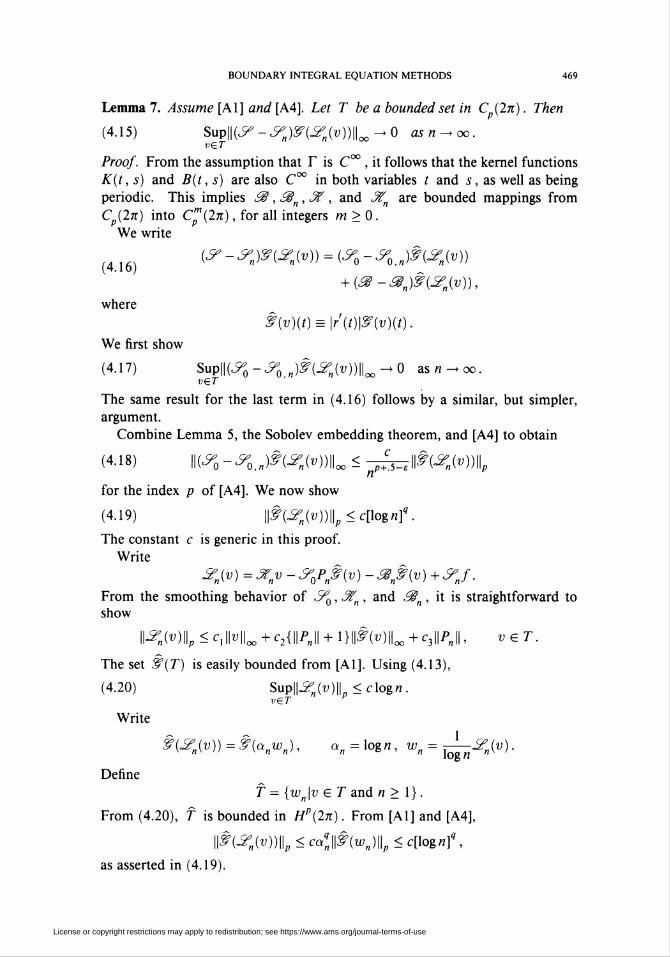
BOUNDARY INTEGRAL EQUATION METHODS 469
Lemma 7. Assume [Al] and [A4]. Let T be a bounded set in C (2k) . Then
(4.15) SuplK^-^S^WJIL^O asn^œ.v€iT
Proof. From the assumption that Y is C°° , it follows that the kernel functions
K(t, s) and B(t, s) are also C°° in both variables t and s, as well as being
periodic. This implies ¿$, 38„ , 3Í, and 3?„ are bounded mappings from
C (27i) into Cp(2n), for all integers m > 0.
We write
(416) i^-ynm^niv)) = (^-^ß(5fn(v))
+ (¿8-3$ß(S?n(v)),
where
§(v)(t) = \r'(tW(v)(t).
We first show
(4.17) SuplK^-^J^i^lL^O as«-oo.veT
The same result for the last term in (4.16) follows by a similar, but simpler,
argument.
Combine Lemma 5, the Sobolev embedding theorem, and [A4] to obtain
(4.18) IK^o -^o,*)^»)IL < ;^ll£(-W)ll,
for the index p of [A4], We now show
(4.19) \\§(S?n(v))\\p<c[logn]q.
The constant c is generic in this proof.
Write
^n(v)=JTnv-^pß(v)-S§ß(v)+^nf.
From the smoothing behavior of S^, 3?„ , and 3§n , it is straightforward to
show
H-Wllp < C. Halloo + ̂ IKH + WMIL + ̂ ll^ll - "G T.
The set &(T) is easily bounded from [Al]. Using (4.13),
(4.20) Suplid (u)||<c log«.ver v
Write
§(5fn(v))=§(a„wn), a„ = logn, w„ = ¿-W-
Define
f = {w„\v gT and n > 1}.
From (4.20), f is bounded in Hp(2k) . From [Al] and [A4],
||f(^„(t;))||p<ca*||#(u7„)||p<c[log«]?,
as asserted in (4.19).
License or copyright restrictions may apply to redistribution; see https://www.ams.org/journal-terms-of-use
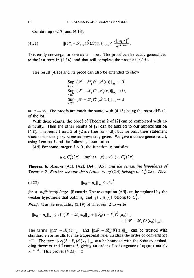
470 K. E. ATKINSON AND GRAEME CHANDLER
Combining (4.19) and (4.18),
(4.21) ||(^0 -^0,„)f (-2>))IL < ̂ St ■
This easily converges to zero as n —► oo. The proof can be easily generalized
to the last term in (4.16), and that will complete the proof of (4.15). D
The result (4.15) and its proof can also be extended to show
«W-^(«))IL-*o,
^W»)IL-o,
jr„):r(.2>))lL-o
as n —* oo. The proofs are much the same, with (4.15) being the most difficult
of the lot.
With these results, the proof of Theorem 2 of [2] can be completed with no
difficulty. Then the other results of [2] can be applied to our approximation
(4.8). Theorems 1 and 2 of §2 are true for (4.8); but we omit their statement
since it is exactly the same as previously given. We give a convergence result,
using Lemma 5 and the following assumption.
[A5] For some integer X > 0, the function g satisfies
ugCp(2k) implies g(-,u(-)) gCç(2k) .
Theorem 8. Assume [Al], [A2], [A4], [A5], and the remaining hypotheses of
Theorem 2. Further, assume the solution uQ of (2.4) belongs to Cp(2k). Then
(4.22) IK-"Joo<<7""
for n sufficiently large. [Remark: The assumption [A5] can be replaced by the
weaker hypothesis that both w0 and g(-, u0(-)) belong to Cp .]
Proof. Use the inequality (2.19) of Theorem 2 to write
IK - "«IL < yiWi* - ̂ >olL +1W - W"o)IL+ \\i&-&nmu0)\\oo}.
The terms ||(JT - ^)"0IL and IK*^ ~ ^)^(Mo)IL can be treated withstandard error results for the trapezoidal rule, yielding the order of convergence
n~k . The term ||<5^(/ - ^¡)^("0)IL can l3e bounded with the Sobolev embed-
ding theorem and Lemma 5, giving an order of convergence of approximately
n-x-.5 This proves (422). d
SuplK^-ver
supiipr-veT
Supiipr-ver
License or copyright restrictions may apply to redistribution; see https://www.ams.org/journal-terms-of-use
BOUNDARY INTEGRAL EQUATION METHODS 471
Table 7
Using method (4.8) to solve (1.4) with g = gx
a b n IK-hJL it COND1.0 2.0 3 2.23E-1 5 5.16
6 1.21E-3 6 4.759 2.77E-6 6 5.26
12 3.53E-9 6 5.3615 2.66E-12 6 5.21
1.0 5.0 5 4.59E-1 6 16.510 1.74E-3 6 15.0
15 3.06E-5 6 16.620 5.57E-7 6 17.6
25 9.79E-9 6 17.930 1.70E-10 6 18.5
1.0 8.0 30 1.75E-6 6 35.6
Table 8
Using method (4.8) to solve (1.4) with g = g2
a b n IK-mJL it COND1.0 2.0 3 1.45E-1 9 780
6 8.27E-4 9 6319 1.82E-6 9 609
12 3.59E-9 9 64315 2.38E-12 9 626
Examples. Consider again the cases (2.21), (2.22) of g, which were used in the
examples of §§2 and 3. The equation (4.8) reduces to a finite system of 2« + 1
nonlinear equations. This system was solved with Newton's method, with the
initial guess
u(? = u0+l, PGY.
The numerical results for various (a, b) and n are given in Tables 7 and 8.
For the meaning of IT and COND, see the discussion for Tables 1 and 2.
The method (4.8) converges very rapidly as n increases, and it is much more
rapid in convergence than the quadratic product integration method of §2. It
can be seen from the tables that the rate of convergence is exponential for
both problems being solved. Using method (4.8), more elongated and difficult
boundaries Y can be treated very accurately with much smaller values of n
than is possible with the quadratic product integration method.
Conclusions
Although the examples in this paper were all computed on elliptical re-
gions, we did similar calculations on other regions with a smooth boundary.
License or copyright restrictions may apply to redistribution; see https://www.ams.org/journal-terms-of-use
472 K. E. ATKINSON AND GRAEME CHANDLER
The numerical results were comparable to those given here, including the much
greater accuracy obtained with the trigonometric product integration method
of §4. We conclude that when the boundary curve is smooth, as in this paper,
then the method of §4 is much superior to the piecewise polynomial product
integration method of §2. If the method of §2 is to be used, then the two-grid
methods of §3 are a very efficient way to solve the nonlinear systems that arise
in the method, and they are preferable to either the ordinary Newton method
or the modified Newton method.
In future papers, the ideas of §§2 and 3 will be extended to planar problems
on regions whose boundary is only piecewise smooth.
Bibliography
1. E. Allgower, K. Böhmer, F. Potra, and W. Rheinboldt, A mesh-independence principle op-
erator equation and their discretizations, SIAM J. Numer. Anal. 23 (1986), 160-169.
2. K. Atkinson, The numerical evaluation of fixed points for completely continuous operators,
SIAM J. Numer. Anal. 10 (1973), 799-807.
3. _, Iterative variants of the Nyström method for the numerical solution of integral equa-
tions, Numer. Math. 22 (1973), 17-31.
4. _, A survey of numerical methods for the solution of Fredholm integral equations of the
second kind, SIAM, Philadelphia, Pa., 1976.
5. F. de Hoog and R. Weiss, Asymptotic expansions for product integration, Math. Comp. 27
(1973), 295-306.
6. M. Krasnoselskii, Topological methods in the theory of nonlinear integral equations, MacMil-
lan, New York, 1964.
7. R. Kress, Boundary integral equations in time-harmonic acoustic scattering, Tech. Rep. #66,
Institut für Numerische und Angewandte Mathematik, Universität Göttingen, 1989.
8. K. Ruotsalainen and W. Wendland, On the boundary element method for some nonlinear
boundary value problems, Numer. Math. 53 (1988), 299-314.
9. Y. Yan and I. Sloan, On integral equations of the first kind with logarithmic kernels, J.
Integral Equations Appl. 1 (1988), 549-579.
10. A. Zygmund, Trigonometric series, Vols. I and II, Cambridge Univ. Press, Cambridge, 1959.
Department of Mathematics, University of Iowa, Iowa City, Iowa 52242
E-mail address: [email protected]
Department of Mathematics, University of Queensland, St. Lucia, Queensland 4067,
Australia
E-mail address: [email protected]
License or copyright restrictions may apply to redistribution; see https://www.ams.org/journal-terms-of-use
![Smoothed Boundary Method for Solving Partial Di erential ... · ux boundary condition can be imposed; the resulting equation is similar to those proposed in Refs. [2, 3, 12, 15]](https://img.pdfslide.net/doc/110x75/5ff5c91d74005c64081a10e2/smoothed-boundary-method-for-solving-partial-di-erential-ux-boundary-condition.jpg)