BOUNDARY LAYER FLOW DUE TO A MOVING FLAT PLATE IN

BOUNDARY LAYER FLOW DUE TO A MOVING FLAT PLATE IN MICROPOLAR FLUID 67

Jurnal Teknologi, 43(C) Dis. 2005: 67–83© Universiti Teknologi Malaysia

BOUNDARY LAYER FLOW DUE TO A MOVING FLAT PLATEIN MICROPOLAR FLUID

MOHD ZUKI SALLEH1, AZIZAH MOHD ROHNI2 & NORSARAHAIDA AMIN3

Abstract. The mathematical model for a boundary layer flow due to a moving flat plate inmicropolar fluid is discussed. The plate is moving continuously in the positive x-direction with aconstant velocity. The governing boundary-layer equations are solved numerically using an implicitfinite-difference scheme. Numerical results presented include the reduced velocity profiles, gyrationcomponent profiles and the development of wall shear stress. The results obtained, when thematerial parameter K = 0 (Newtonian fluid) showed excellent agreement with those for viscousfluids. Further, the wall shear stress increases with increasing K. For fixed K, the wall shearstress decreases and the gyration component increases with increasing values of n, in the range0 ≤ n ≤ 1 where n is a ratio of the gyration vector component and the fluid shear stress at the wall.

Keywords: Boundary layer, micropolar fluid, moving flat plate, Keller-box method, mathematicalmodel

Abstrak. Pemodelan matematik bagi aliran lapisan sempadan terhadap plat rata bergeraktelah dibincangkan. Satu plat bergerak berterusan dalam arah positif paksi-x dengan halaju tetap.Persamaan lapisan sempadan yang dihasilkan telah diselesaikan secara berangka denganmenggunakan skema beza terhingga tersirat. Keputusan berangka telah diberikan, ini termasukprofil halaju, profile komponen legaran dan perubahan tegasan ricih permukaan. Kajian inimenunjukkan bahawa keputusan bagi masalah dalam bendalir mikropolar berbanding denganbendalir likat adalah sangat memuaskan apabila parameter bahan K = 0 (bendalir Newtonan).Seterusnya tegasan ricih permukaan meningkat dengan peningkatan nilai K. Untuk nilai K yangditetapkan, didapati tegasan ricih permukaan menyusut dan kompenan legaran meningkat denganpeningkatan nilai n, dalam selang 0 ≤ n ≤ 1, di mana n adalah nisbah kompenan vektor legarandengan tegasan ricih bendalir pada permukaan.

Kata kunci: Lapisan sempadan, bendalir mikropolar, plat rata bergerak, kaedah Keller-box,pemodelan matematik

1 Faculty of Mechanical Engineering, Kolej Universiti Kejuruteraan dan Teknologi Malaysia, BandarMEC, 25500 Gambang, Kuantan, Pahang. E-mail: [email protected]

2 Faculty of Quantitative Sciences, Universiti Utara Malaysia, 06010 UUM Sintok, Kedah. E-mail:[email protected]

3 Department of Mathematics, Universiti Teknologi Malaysia, 81310 UTM Skudai, Johor. E-mail:[email protected]

JTDIS43C[05].pmd 02/15/2007, 16:1267

MOHD ZUKI SALLEH, AZIZAH MOHD ROHNI & NORSARAHAIDA AMIN68

1.0 INTRODUCTION

The boundary-layer flow over a moving continuous solid surface is important inseveral engineering processes. For example, materials manufactured by extrusionprocesses and heat-treated materials travelling between a feed roll and a wind-uproll or on conveyor belt possess the characteristics of a moving continuous surface.Sakiadis [1] first investigated the boundary-layer flow on a continuous solid surfacemoving at constant speed. Due to the entrainment of the ambient fluid, this boundary-layer flow is quite different from the Blasius flow past a flat plate. Sakiadis’ theoreticalpredictions for Newtonian fluids were later corroborated experimentally by Tsouet al. [2]. Lee and Davis [3] investigated the laminar boundary layers on movingcontinuous surfaces while the turbulent boundary layer on a moving continuousplate was studied by Noor Afzal [4].

This paper will investigate the boundary layer flow due to a moving flat plate inboth viscous and micropolar fluids. A micropolar fluid is one which containssuspensions of rigid particles such as blood, liquid crystals, dirty oil and certaincolloidal fluids, which exhibits microstructure. The theory of such fluids was firstformulated by Eringen [5]. The equations governing the flow of a micropolar fluidinvolve a microrotation vector and a gyration parameter in addition to the classicalvelocity vector field. This theory includes the effects of local rotary inertia and couplestresses and is expected to provide a mathematical model for the non-Newtonianbehavior observed in certain man-made liquids such as polymeric fluids and innaturally occurring liquids such as animal blood. The theory of thermomicropolarfluids was also developed by Eringen [6] by extending the theory of micropolarfluids. A comprehensive review of micropolar fluid mechanics was given by Arimanet al. [7]. Their studies on the inadequacy of the classical Navier-Stokes theory todescribe rheologically complex fluids such as liquid crystals, animal blood, etc., hasled to the development of microcontinuum fluid mechanics as an extension of theclassical theory. Many models have been proposed to take into account themechanically significant microstructure of such fluids. Rees and Bassom [8] haveconsidered the Blasius boundary layer flow of a micropolar fluid over a flat plate,while a similarity analysis of the flow and heat transfer past a continuously movingsemi-infinite plane in micropolar fluid has been presented by Soundalgekar andTakhar [9].

This paper will also consider the problems of the boundary-layer flow. We deriveand solve the full boundary layer equations. The analyses involve the pseudo-similaritytransformation of the governing equations and the resulting nonlinear equations arethen solved using an implicit finite difference scheme, the Keller-box method. Thereduced velocity, reduced gyration component and development of wall shear stressare shown by means of graphs.

JTDIS43C[05].pmd 02/15/2007, 16:1268


2.0 GOVERNING EQUATIONS

Consider the flow of a steady, laminar, incompressible micropolar fluid past anextensible sheet, which is moving continuously in the positive x – direction with anarbitrary surface velocity U. The orthogonal coordinates x , y are measured alongthe sheet and, respectively, normal to it with the origin at a fixed point 0.

The full equations governing the two-dimensional steady flow of a micropolarfluid are (Ahmadi [10]):

0u vx y

∂ ∂+ =∂ ∂

(1)

2 2

2 2

1u u p u u Nu v

x y x x y yκ κµ

ρ ρ ρ ∂ ∂ ∂ ∂ ∂ ∂ + = − + + + + ∂ ∂ ∂ ∂ ∂ ∂

(2)

2 2

2 2

1v v p v v Nu v

x y x x y yκ κµ

ρ ρ ρ ∂ ∂ ∂ ∂ ∂ ∂ + = − + + + + ∂ ∂ ∂ ∂ ∂ ∂

(3)

2 2

2 22N N u v N N

u v Nx y y x x y

κ κ γρζ ρζ ρζ

∂ ∂ ∂ ∂ ∂ ∂ + = − + + + + + ∂ ∂ ∂ ∂ ∂ ∂ (4)

Following Ahmadi [10], ( x , y ) are the coordinates parallel with and perpendicularto the flat surface, (u ,v ) is the velocity vector, p is the pressure, N is the componentof the gyration vector normal to the x – y plane, and ζ is the microinertia density.Further, ρ is the fluid density, µ is the viscosity, κ is the microrotation parameter(also known as the coefficient of gyroviscosity or as the vortex viscosity) and γ is thespin-gradient viscosity. We follow the work of many recent authors by assuming thatζ is a constant. The Equations (1), (2), (3) and (4) are to be solved subject to:

0 on 0u

v , u U , N n yy

∂→ = = − =∂ (5a)

0 0 0 asu , v , N y→ → → → ∞ (5b)

In Equation (5a) we have followed Arafa and Gorla [11] in assigning a variablerelation between N and the skin friction at the surface. The value n = 0, representsconcentrated particle flows in which the microelements close to the wall are unable

to rotate. The value 12

n = is indicative of weak concentration, and when n = 1, is

used for the modeling of turbulent boundary layer. We shall consider values of n

which lie between these two extremes.

JTDIS43C[05].pmd 02/15/2007, 16:1269


We introduce now the nondimensional variables:

2

1yx u v px , y ,u ,v , p ,N N

l l U U U Uρ = = = = = =

(6)

and follow Ahmadi [10] to assume that γ is given by,

2,

κγ µ ζ = + (7)

We obtain from Equations (1) – (4) the following:

0u vx y

∂ ∂+ =∂ ∂

(8)

2 2

2 2

1 K KRe Re

u u p u u Nu v

x y x x y y ∂ ∂ ∂ + ∂ ∂ ∂ + = − + + + ∂ ∂ ∂ ∂ ∂ ∂

(9)

2 2

2 2

1 K KRe Re

v v p v v Nu v

x y y x y x

∂ ∂ ∂ + ∂ ∂ ∂ + = − + + − ∂ ∂ ∂ ∂ ∂ ∂ (10)

2 2

2 2

K1K K 22

ReN N l u l N N N

u v Nx y U y U x x yρζ ρζ

+ ∂ ∂ ∂ ∂ ∂ ∂ + = − + − + + ∂ ∂ ∂ ∂ ∂ ∂ (11)

where K is the material parameter defined by Kκµ

= and Re is the Reynolds number

defined by ReUlv

= . If we take 2lζ = as a reference length scale for ζ, then (11)

becomes:

2 2

2 2

K1K K 22

Re Re ReN N u N N N

u v Nx y y x x y

+ ∂ ∂ ∂ ∂ ∂ ∂ + = − + − + + ∂ ∂ ∂ ∂ ∂ ∂ (12)

The boundary conditions (5) become:

0 1 on 0du

v , u , N n ydy

→ = = − = (13a)

0 0 0 asu , v , N y→ → → → ∞ (13b)

JTDIS43C[05].pmd 02/15/2007, 16:1270


Now we introduce the boundary layer variables:1 1 12 2 2Re Re ReX x, Y y, U u, V v, N N= = = = = (14)

into Equations (8), (9), (10) and (12) to obtain:

0U VX Y

∂ ∂+ =∂ ∂

(15)

2 2

2 2

1(1+ K) K

ReU U p U U N

U VX Y X X Y Y

∂ ∂ ∂ ∂ ∂ ∂+ = − + + + ∂ ∂ ∂ ∂ ∂ ∂ (16)

2 2

2 2 2 2

1 1 1 K(1+ K)

Re Re Re ReV V p V V N

UX Y Y X Y X

∂ ∂ ∂ ∂ ∂ ∂ + = − + + − ∂ ∂ ∂ ∂ ∂ ∂ (17)

1 1 32 2 2

1 2 22

2 2

Re K Re 2 K Re

K 11 Re

2 Re

N N U NU V N

X Y Y X

N NX Y

− − −

−

∂ ∂ ∂ ∂ + = − + − ∂ ∂ ∂ ∂ ∂ ∂ + + + ∂ ∂

(18)

Taking Re → ∞ as boundary layer approximation, we have:

0U VX Y

∂ ∂+ =∂ ∂

(19)

( )2

21 K KU U p U N

U VX Y X Y Y

∂ ∂ ∂ ∂ ∂+ = − + + +∂ ∂ ∂ ∂ ∂

(20)

0pY

∂= −∂ (21)

2

2

KK 2 1

2N N U N

U V NX Y Y Y

∂ ∂ ∂ ∂ + = − + + + ∂ ∂ ∂ ∂ (22)

The boundary conditions (13) reduce to:

0 1 on 0U

V , U , N n YY

∂= = = − =∂ (23a)

0 0 asU , N Y= → → ∞ (23b)

Equation (21) shows that p = p(x) and Equation (20), on applying the boundarycondition (23b), gives:

JTDIS43C[05].pmd 02/15/2007, 16:1271


0pX

∂ =∂

Finally, we have the following boundary layer equations for the problem underconsideration:

0U VX Y

∂ ∂+ =∂ ∂ (24)

( )2

21 KU U U N

U V KX Y Y Y

∂ ∂ ∂ ∂+ = + +∂ ∂ ∂ ∂

(25)

2

21 2N+2

N N K N UU V K

X Y Y Y∂ ∂ ∂ ∂ + = + − ∂ ∂ ∂ ∂

(26)

subject to the boundary conditions

0 1 on 0U

V , U , N n YY

∂= = = − =∂

0 0 asU , N Y= → → ∞ (27)

we define the reduced stream function, f, the reduced gyration component, g, andthe pseudo-similarity variable, η as:

( ) ( )1 1 12 2 2f X , X , g X , X N , X Yη ψ η η− −= = = (28)

where ψ is the stream function which satisfies:

U , VY Xψ ψ∂ ∂= = −

∂ ∂ (29)

When the stream function ψ is introduced, the continuity Equation (24) isautomatically satisfied. We obtain from (25) and (26):

( )3 2 2 2

3 2 2

11 K K

2f f f f f fg

f XX Xη η η η η η

∂ ∂ ∂ ∂ ∂ ∂∂+ + + = − ∂ ∂ ∂ ∂ ∂ ∂ ∂ ∂ (30)

22

2 2

K 11 K 2

2 2

f fg gf g X g

f fg gX

X X

η η η η

η η

∂ ∂∂ ∂ + + + = + ∂ ∂ ∂ ∂ ∂ ∂∂ ∂ + − ∂ ∂ ∂ ∂

(31)

JTDIS43C[05].pmd 02/15/2007, 16:1272


with the boundary conditions

2

20 1 on 0f f

f , , g n ηη η

∂ ∂= = = − =

∂ ∂ (32a)

0 0 asf

, g .ηη

∂ → → → ∞∂ (32b)

Thus we have derived a set of parabolic partial differential equations which governthe development of the boundary layer, which in general, requires numericalsolution.

Before presenting the computed results, it is convenient to draw attention to twocases for which Equations (30), (31) and boundary conditions (32) admit similarity

solutions [8]. Similarity solution arises when 12

n = . We can take:

( ) ( ) ( )0 0and 0f X , f g X , gη η η= = =

where f0 and g0 are obtained from (30) and (31) as:

( )0 0 0 0

11 K K 0

2''' " 'f f f g+ + + = (33)

0 0

12

''g f= − (34)

If we substitute Equation (34) into (33), we get:

0 0 0

K 11 0

2 2' ''f f f + + = (35)

subject to:

( ) ( )

( )0 0

0

0 0 0 1 on 0

0 as

'

'

f , f

f

ηη

= = =

∞ → → ∞ (36)

Now we set:

( ) ( )1 12 2

0 0

K K1 1

2 2f f ,η η η η

− = + = +

(37)

Hence that Equation (35) reduces to:

0 0 0

10

2''' ''f f f+ = (38)

JTDIS43C[05].pmd 02/15/2007, 16:1273


subject to:

( ) ( )

( )00

0

0 0 0 1 on 0

0 as

'

'

f , f

f

η

η

= = =

∞ = → ∞ (39)

Equations (38) and (39) describe the flow due to a moving flat plate in a quiescentfluid first described by Sakiadis [1].

Following Rees and Bassom [8], a second similarity solution arises when K = 0 forwhich

( ) ( ) ( ) ( )( )1

2 0and 0f s ds''f f g nf e

η

η η η− ∫= = − (40)

In this case, the flow field is unaffected by the microstructure of the fluid, and hencethe gyration component is a passive quantity.

3.0 NUMERICAL SOLUTION

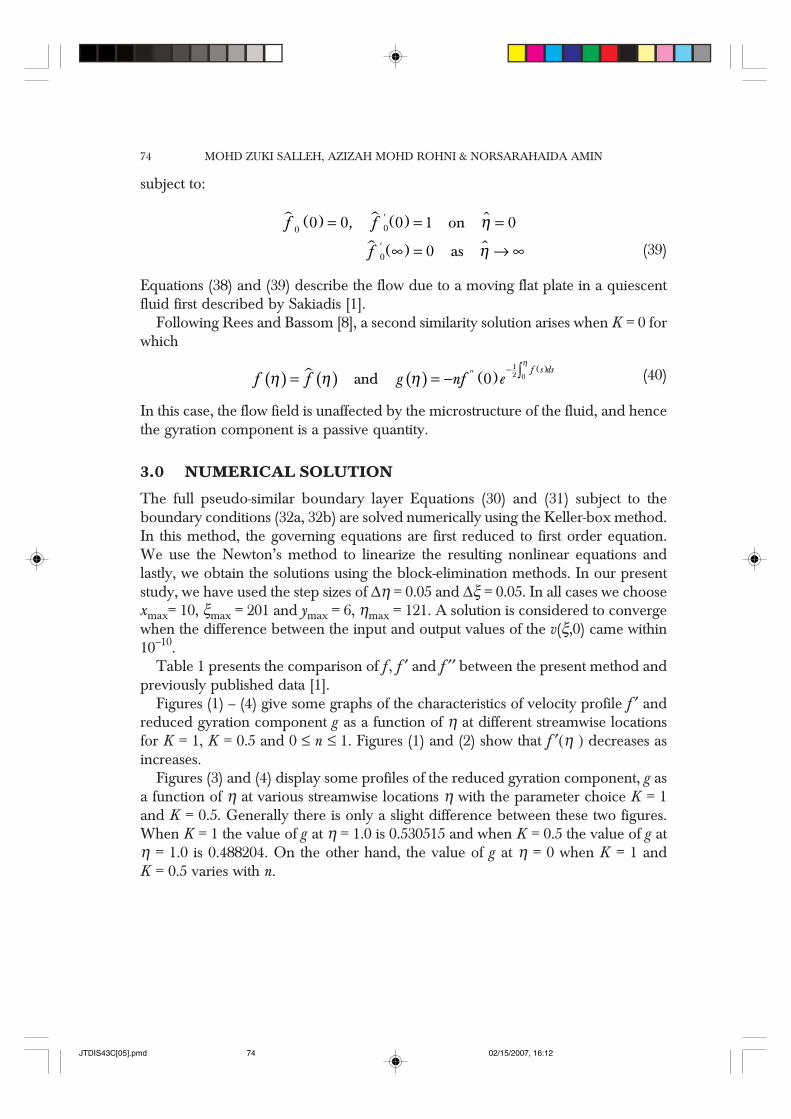
The full pseudo-similar boundary layer Equations (30) and (31) subject to theboundary conditions (32a, 32b) are solved numerically using the Keller-box method.In this method, the governing equations are first reduced to first order equation.We use the Newton’s method to linearize the resulting nonlinear equations andlastly, we obtain the solutions using the block-elimination methods. In our presentstudy, we have used the step sizes of ∆η = 0.05 and ∆ξ = 0.05. In all cases we choosexmax= 10, ξmax = 201 and ymax = 6, ηmax = 121. A solution is considered to convergewhen the difference between the input and output values of the v(ξ,0) came within10–10.

Table 1 presents the comparison of f, f ′ and f ′′ between the present method andpreviously published data [1].

Figures (1) – (4) give some graphs of the characteristics of velocity profile f ′ andreduced gyration component g as a function of η at different streamwise locationsfor K = 1, K = 0.5 and 0 ≤ n ≤ 1. Figures (1) and (2) show that f ′(η ) decreases asincreases.

Figures (3) and (4) display some profiles of the reduced gyration component, g asa function of η at various streamwise locations η with the parameter choice K = 1and K = 0.5. Generally there is only a slight difference between these two figures.When K = 1 the value of g at η = 1.0 is 0.530515 and when K = 0.5 the value of g atη = 1.0 is 0.488204. On the other hand, the value of g at η = 0 when K = 1 andK = 0.5 varies with n.

JTDIS43C[05].pmd 02/15/2007, 16:1274


Table 1 Comparison between Sakiadis [1] and the present method for the similar flow

eta(eta(eta(eta(eta(hhhhh ))))) fffff fffff ¢¢¢¢¢ fffff ¢¢¢¢¢¢¢¢¢¢

0.00 present 0.000000 1.000000 –0.443920(Sakiadis) (0.00000) (1.00000) (–0.44375)






1

Figure 1 Profile of the reduced streamwise velocity f ′ as a function of η at different streamwiselocation for K = 1 and for 0 ≤ n ≤ 1

0.8

0.6

0.4

0.2

00

n = 0.0n increasing

K = 1

n = 0.1

f’

21 3 4 5 6

hhhhh

0.9

0.7

0.5

0.3

0.1

JTDIS43C[05].pmd 02/15/2007, 16:1275


Figure 2 Profile of the reduced streamwise velocity f ′ as a function of η at different streamwiselocation for K = 0.5 and for 0 ≤ n ≤ 1

Figure 3 Profile of the reduced gyration component g as a function of η at different streamwiselocations for K = 1 and for 0 ≤ n ≤ 1

0.6

0

hhhhh

n = 1.0

K = 1

n = 0.0n = 0.1n = 0.2n = 0.3

n = 0.4n = 0.5n = 0.6n = 0.7

n = 0.8n = 0.9

0.1

0.2

0.3

0.4

0.5

0.7

01 2 3 4 5 6

ggggg

1

0.8

0.6

0.4

0.2

00

f’

21 3 4 5 6

hhhhh

n = 0.0n increasing

K = 0.5

n = 0.1

JTDIS43C[05].pmd 02/15/2007, 16:1276


Figures (5) - (8) illustrate the variation of the shear stress (or skin friction) and therate of change of gyration component at the solid boundary with X. Figures (5)and (6) plot f ′′ at η = 0 as a function of X for various values of K, and for n = 0 and

Figure 4 Profile of the reduced gyration component g as a function of η at different streamwiselocations for K = 0.5 and for 0 ≤ n ≤ 1

Figure 5 Development of the wall shear stress f ′′(X, 0) as a function of X for n = 0 and for variousvalues of K

K = 3

–0.1

0

f ′′′′′′′′′′(X, 0)

1 2 3 4 5 6 7 8 9 10

K = 10

K = 5

K = 1.0

K = 0.5

K = 0.3

K = 0.1K = 0

X

–0.15

–0.2

–0.25

–0.3

–0.35

–0.4

–0.45

0

n = 0.2

n = 0.3

01 2

n = 0.1n = 0.0

n = 0.4

n = 0.5

n = 0.6

n = 0.7

n = 0.8

n = 0.9

n = 1.0

0.05

0.1

0.15

0.2

0.25

0.3

0.35

0.4

0.45

0.5

3 4 5 6

K = 0.5

hhhhh

ggggg

JTDIS43C[05].pmd 02/15/2007, 16:1277


n = 0 . For fixed n, increasing value of f ′′ would seem to be associated with increasingvalue of K and when K = 0 the curves are very approximately or closed to beinghorizontal lines.

Figure 6 Development of the wall shear stress f ′′(X, 0) as a function of X for n = 1 and for variousvalues of K

–0.3

–0.4

–0.5

–0.6

–0.7

–0.8

–0.9

K = 0.3K = 0.1K = 0

K = 0.5K = 1

K = 3

K = 5

K = 1021.81.61.41.210.80.60.40.20

X

f ′′′′′′′′′′(X, 0)

n = 1

Figure 7 Development of the rate of change of the gyration component at the wall g′(X, 0) as afunction of X for η = 0 and for various values of K

0.7

K = 0.1

X

g′′′′′(X, 0)

0.6

0.5

0.4

0.3

0.2

0.1

00 1 2 3 4 5 6 7 8 9 10

K = 0

K = 0.3

K = 3K = 5K = 0.5K = 10

n = 0

K = 1

JTDIS43C[05].pmd 02/15/2007, 16:1278


Figures (7) and (8) show the rate of change of the gyration component at the wall,g′′(X, 0) for different values of K.

Figures (9) - (12) consider the development of the wall shear stress, f ′′(X, 0) andthe rate of change of the gyration component at the wall, g′(X, 0) with X. The figures

Figure 8 Development of the rate of change of the gyration component at the wall g′(X, 0) as afunction of X for η = 1 and for various values of K

g′′′′′(X, 0)

0

–0.5

–1

–1.5

–2

–2.5

–3

–3.5

–4

–4.5

X

0 1 2 3 4 5 6 7 8 9 10K = 10

K = 5

K = 3

K = 1

K = 0.5K = 0.3K = 0.1K = 0

n = 1

Figure 9 Development of the wall shear stress f ′′(X, 0) as a function of X for K = 0.5 and a rangeof values of n

X

0 1 2 3 4 5 6 7 8 9 10

n = 1.0

f ′′′′′′′′′′(X, 0)

–0.32

–0.42

–0.4

–0.38

–0.36

–0.34

–0.44

–0.46

–0.48

–0.5

n = 0.9

n = 0.8

n = 0.7

n = 0.6

n = 0.5

n = 0.4

n = 0.3n = 0.2n = 0.1n = 0.0

K = 0.5

JTDIS43C[05].pmd 02/15/2007, 16:1279


present the corresponding graphs when K = 0.5 and K = 1 is taken, and n is varied

between 0 and 1. The similarity solution corresponding to 12

n = is evident as a

straight line in all these figures.

Figure 10 Development of the wall shear stress f ′′(X, 0) as a function of X for K = 1 and a rangeof values of n

X

0 1 2 3 4 5 6 7 8 9 10

n = 1.0

f ′′′′′′′′′′(X, 0)

–0.2

–0.4

–0.35

–0.3

–0.25

–0.45

–0.5

–0.55

n = 0.9

n = 0.8

n = 0.7

n = 0.6

n = 0.5n = 0.4n = 0.3n = 0.2n = 0.1n = 0.0

K = 1

Figure 11 Development of function g′(X, 0) as a function of X for K = 0.5 and a range of valuesof n

X

0 1 2 3 4 5 6 7 8 9 10

n = 1.0

g′′′′′(X, 0)

0.6

–0.2

0

0.2

0.4

–0.4

–0.6

–0.8

n = 0.9

n = 0.8

n = 0.7

n = 0.6

n = 0.5

n = 0.4

n = 0.3n = 0.2

n = 0.1n = 0.0K = 0.5

JTDIS43C[05].pmd 02/15/2007, 16:1380


Figure 12 Development of function g′(X, 0) as a function of X for K = 1 and a range of values ofn

X

0 1 2 3 4 5 6 7 8 9 10

n = 1.0

g′′′′′(X, 0)

0.6

–0.2

0

0.2

0.4

–0.4

–0.6

–0.8 n = 0.9

n = 0.8

n = 0.7

n = 0.6

n = 0.5

n = 0.4n = 0.3n = 0.2n = 0.1n = 0.0

K = 1

–1

–1.2

4.0 CONCLUSION

The governing boundary layer equations are solved numerically using an implicitfinite difference scheme. Numerical results presented include the reduced velocityprofiles, gyration component profiles and the development of wall shear stress orskin friction. These numerical results indicated that a near-wall contact layer develop

as X → ∞ but only if 12

n ≠ . But, when either 12

n = or K = 0, the solution is self-similar and there is no near-wall layer [8]. The results obtained, for the materialparameter K = 0 (Newtonian fluid), are in excellent agreement with those obtainedfor viscous fluids. Further, the wall shear stress increases with increasing K. For fixedK, the wall shear stress decreases and the gyration component increases with increasingvalues of n, in the range 0 ≤ n ≤ 1 where n is a ratio of the gyration vector componentand the fluid shear stress at the wall.

REFERENCES[1] Sakiadis, B. C. 1961. Boundary Layer Behavior Continuous Solid Surfaces: II. The Boundary Layer on a

Continuous Flat Surface. A.I.Ch. E. Journal. 7: 221-225.[2] Tsou, F., E. Sparrow, and R. Goldstein. 1967. Flow and Heat Transfer in the Boundary Layer on a

Continuous Moving Surfaces. Int. J. Heat and Mass Transfer. 10: 219-235.[3] Lee, W. W., and R. T. Davis. 1972. Laminar Boundary Layer on Moving Continuous Surfaces. Chemical

Eng. Science. 27: 2129-2149.[4] Noor Afzal. 1996. Turbulent Boundary Layer on a Moving Continuous Plate. Fluid Dynamic Research. 17:

181-194.[5] Eringen, A. C. 1964. Simple Microfluids. Int. J. Engng. Sci. 2: 205.[6] Eringen, A. C. 1966. Theory of Micropolar Fluid. J. Math. Mech. 16: 1-18.

JTDIS43C[05].pmd 02/15/2007, 16:1381


[7] Ariman, T., M. A. Turk, and N. D. Sylvester. 1973. Microcontinuum Fluid Mechanics- a Review.Int. J. Engng. Sci. 11: 905-930.

[8] Rees, D. A. S., and A. P. Bassom. 1996. The Blasius Boundary Layer Flow of a Micropolar Fluid.Int. J. Engng. Sci. 34: 113-124.

[9] Soundalgekar, V. M., and H. S. Takhar. 1983. Flow of Micropolar Fluid Past a Continuously Moving FlatPlate. Int. J. Engng. Sci. 21: 961-905.

[10] Ahmadi, G. 1976. Self Similar Solution of Incompressible Micropolar Boundary Layer Flow over a SemiInfinite Plate. Int. J. Engng. Sci. 14: 639-646.

[11] Arafa, A. A., and R. S. R. Gorla. 1992. Mixed Convection Boundary Layer Flow of a Micropolar FluidAlong Vertical Cylinders and Needles. Int. J. Engng. Sci. 30: 1745-1751.

NOMENCLATURE

Roman Letters

f – Reduced stream function

f0 – Reduced stream function for 12

n =

f – Reduced stream function for the classical Blasius boundary-layer flow

g – Reduced gyration component

g0 – Reduced gyration component for 12

n =

ζ – Microinertia density

j0 – Reference value of the microinertia density

K – Ratio of the gyroviscosity and the fluid viscosity

l – Length scale

n – Ratio of the gyration vector component and the fluid shear at a solidboundary

N – The gyration vector component perpendicular to the x-y plane

p – Pressure

Re – Reynolds number, oU lρµ

v – Fluid velocity component in y-direction

x – Coordinate along the plate

x – Dimensionless coordinate x

y – Coordinate normal to the plate

y – Dimensionless coordinate y

JTDIS43C[05].pmd 02/15/2007, 16:1382


X, Y – Nondimensional streamwise and cross-stream Cartesian coordinates

u – Dimensionless velocity u

u – Fluid velocity component in x-direction

U – Free stream velocity

v – Dimensionless velocity v

Greek Letters

δ – Boundary layer thickness

η – Pseudo-similarity variable

η – Scaled pseudo-similarity variable

γ – Spin-gradient viscosity

µ – Dynamic viscosity

κ – Coefficient of gyroviscosity

υ – Kinematic viscosity

ξ – Transformed streamwise coordinate

ρ – Density of the fluid

ψ – Stream function

θ – Momentum thickness

Superscripts

′ – Differentiation with respect to– – Dimensional variables

JTDIS43C[05].pmd 02/15/2007, 16:1383

Documents

BOUNDARY LAYER FLOW DUE TO A MOVING FLAT PLATE IN