Boundary layer processesBjorn Stevens

Max Planck Institute for Meteorology, Hamburg

The Atmospheric Boundary Layer (ABL)

• ‘An Abstraction’ (Wippermann ‘76)

• ‘The bottom 100-3000 m of the Troposphere’ (Stull ’94)

• ‘The lower part of the troposphere where the direct influence from the surface is felt through turbulent exchange with the surface’ (Beljaars ’94)

A turbulent layer that emerges due to the destabilizing influence of the surface on the atmosphere, and which is characterized by lengthscales h, such that

z0 << h << H, L

Here z0 denotes the scale of roughness elements, H is the depth of the troposphere and L is the characteristic length scale measuring variations in surface properties

Who cares?

• Spin-down of the large-scale flow (Charney & Eliassen, 1949) --- ‘It is thus noteworthy that the first incorporation of the planetary boundary layer in a numerical prediction model was done even before the first 1-day forecast was made’ (A. Wiin-Nielsen, 1976)

• Conditional Instability of the Second Kind (CISK; Charney & Eliasen, 1964, Ooyama 1964)

• Diurnal Cycle: Convection/Precipitation & Nightime Minimum Temperatures.

• Air Pollution, Contaminant Dispersion.

• Ocean Coupling (wind-stress and wind-stress curl).

• Radiative balance & Hydrological Cycle.

• Modulation of local circulations: mountain-valley flows; sea breezes; katabatic flows.

• Biogeochemical Cycles (nutrient transport in upper ocean/ boundary layer transport).

• Wind Power.

The impact of the boundary layer in models is particularly felt after a few days of integration when the accumulated surface fluxes contribute substantially to the heant, moisture and momentum balance of the atmosphere. (A. Beljaars, 1994)

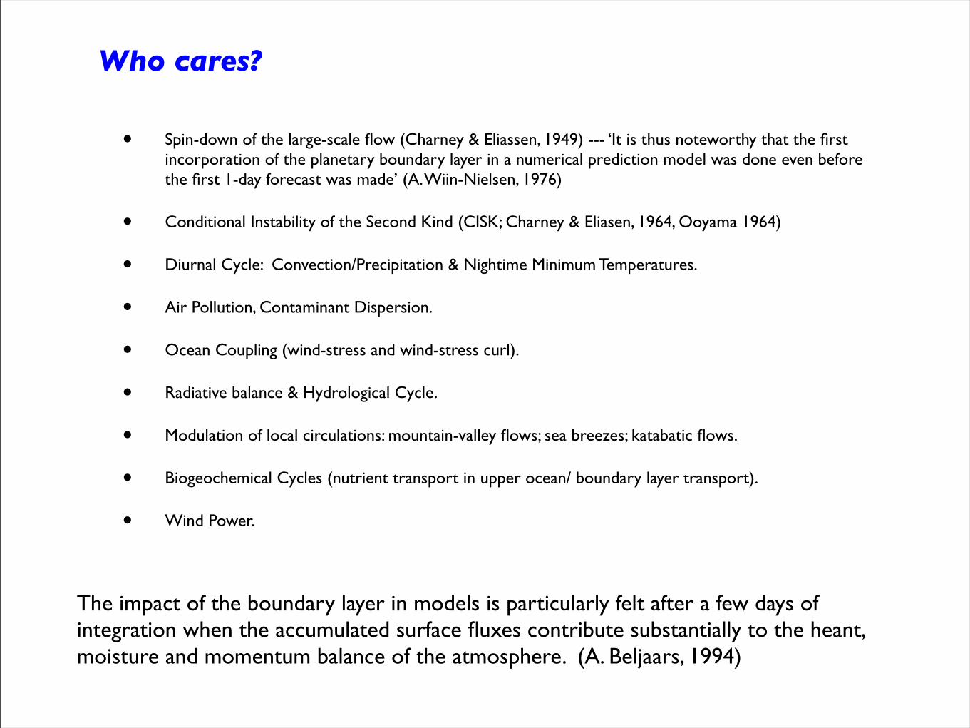
The Boundary Layer -- Prandtl/Blasius

!tu + u ·!u = ""!xp + #!2u (1)

H !" (!x/U)1/2 # (!t)1/2

w ! (!U/x)1/2

!t" + u ·!" = #!2"

The Boundary Layer -- Ekman

!tv + u ·!v + fu = ""!yp + #!2v

H !" (!/f)1/2

The wind vector turns clockwise (veers) with height.

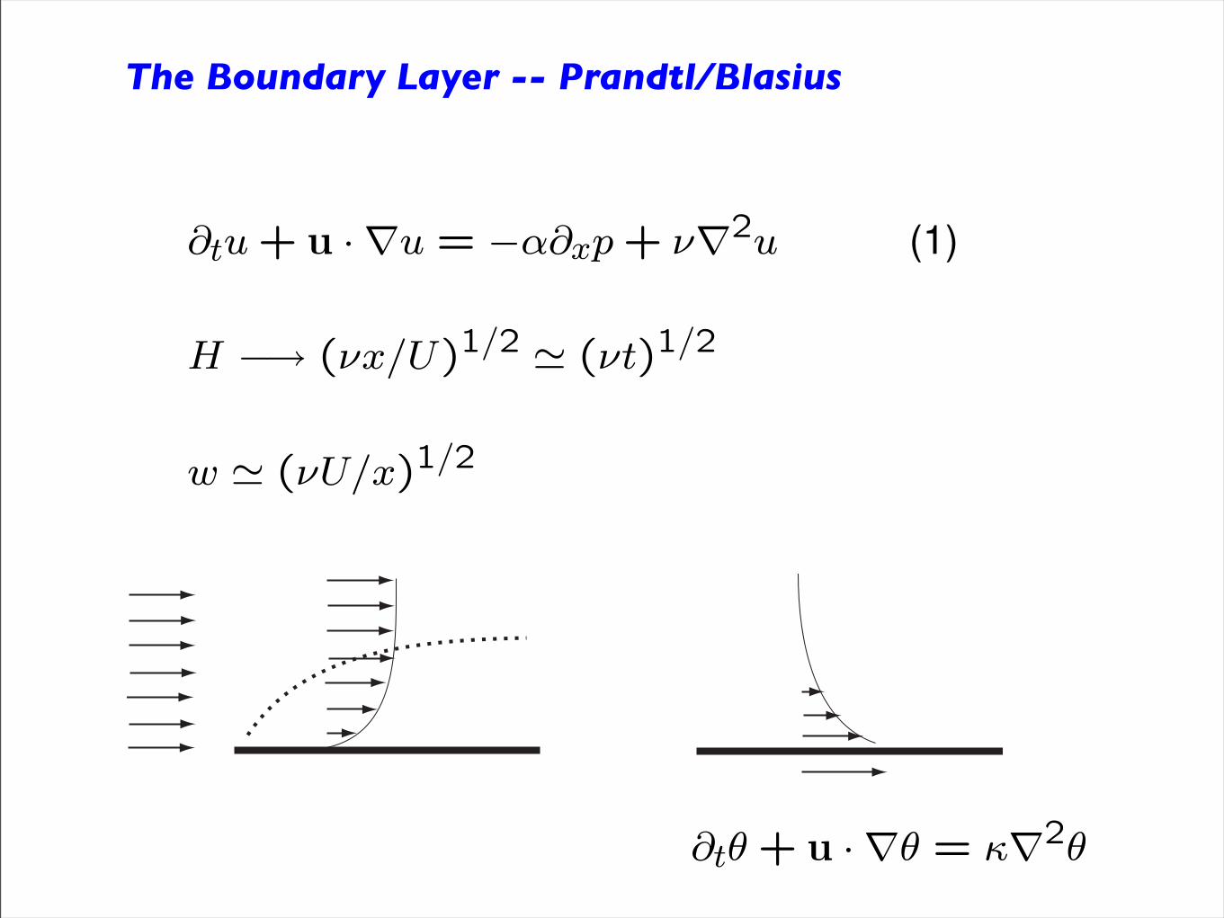
Remarks -- Momentum Boundary Layers

• Concepts: Boundary layer depth, h; Secondary Circulations, w.

• Viscous solutions are unstable, and the surface is not smooth, hence atmospheric boundary layers are turbulent.

!tv + u ·!v + fu = ""!yp + #!2v +! · (A!v)

where

v#u# $ "A!v

! · (A!v) = !A ·!v + A!2v

A = !2!!!!du

dz

!!!!

which introduces the idea of a mixing length, which is reasonable if

!!!!!!du

dz

!!!!

"d2u

dz2

#"1

i.e., mixing is local.

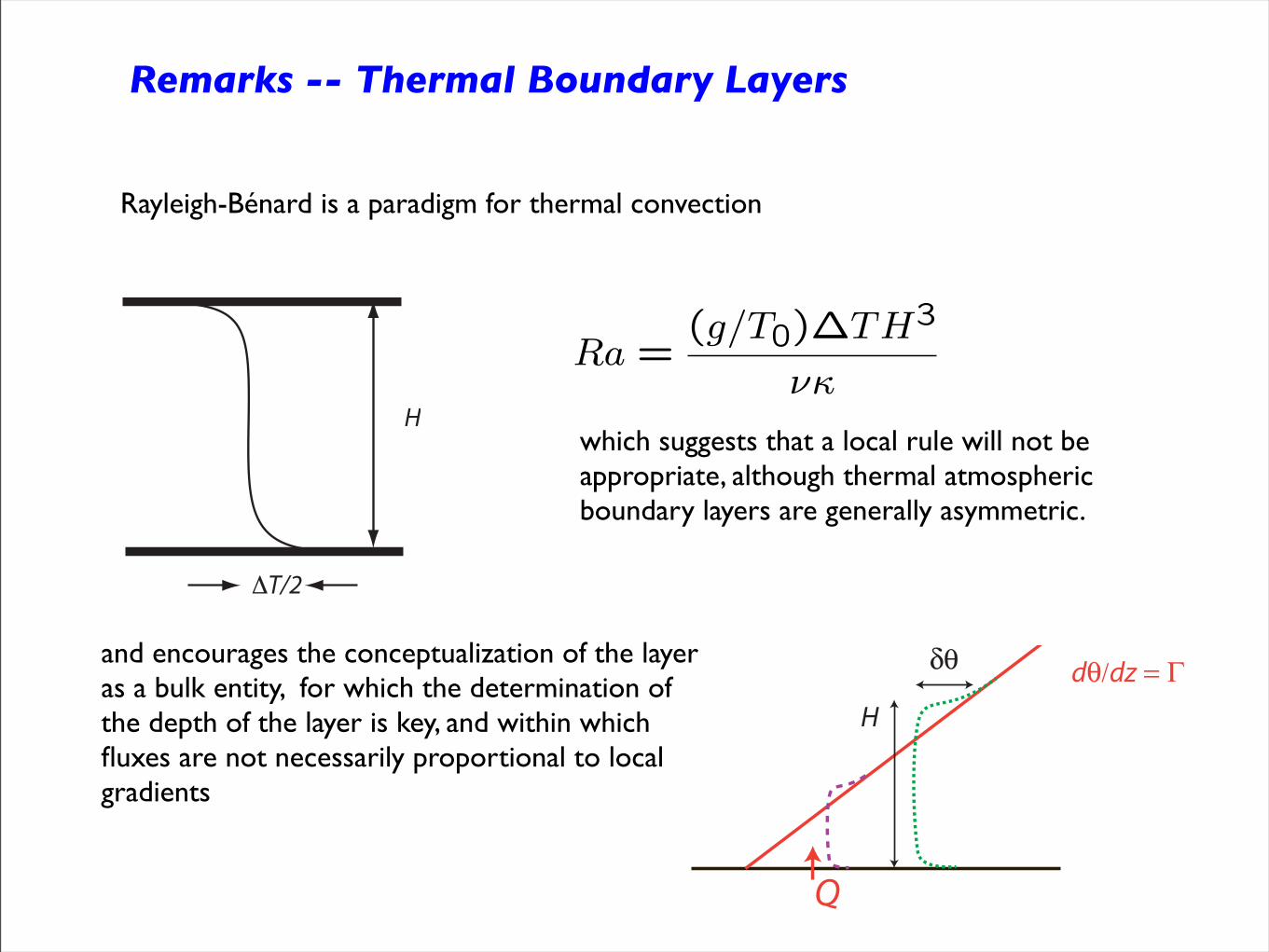
Remarks -- Thermal Boundary Layers

Rayleigh-Bénard is a paradigm for thermal convection

Ra =(g/T0)!TH3

!"

!T/2

Hwhich suggests that a local rule will not be appropriate, although thermal atmospheric boundary layers are generally asymmetric.

and encourages the conceptualization of the layer as a bulk entity, for which the determination of the depth of the layer is key, and within which fluxes are not necessarily proportional to local gradients

Remarks -- Concepts

• Eddy Diffusivity/Viscosity (local concept)

• Mixing Length, l

• Surface matching,

Shear Dominance

Buoyancy Dominance

• Boundary Layer Depth (integral concept)

• Surface layer (z << h),

• Entrainment layer

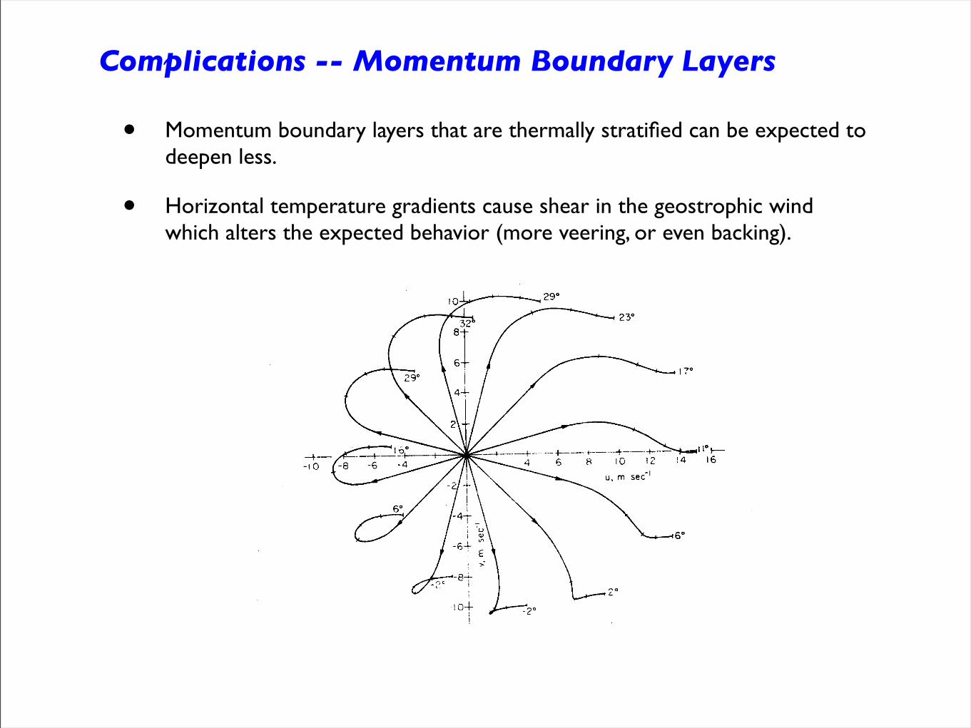
Complications -- Momentum Boundary Layers

• Momentum boundary layers that are thermally stratified can be expected to deepen less.

• Horizontal temperature gradients cause shear in the geostrophic wind which alters the expected behavior (more veering, or even backing).

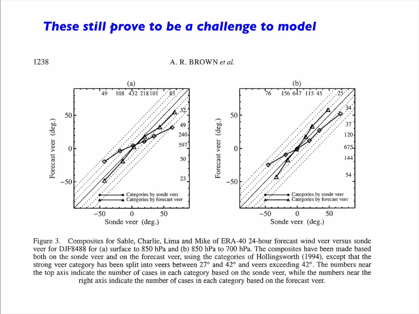
These still prove to be a challenge to model

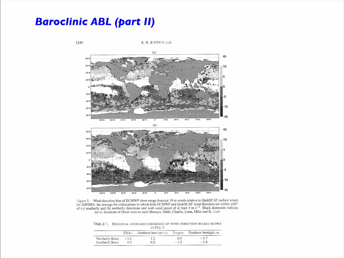
Baroclinic ABL (part II)

Baroclinic ABL (part III)

Model Changes that limit mixing leads to a globally worse model, but one that better agrees with the data locally --- A persistent problem.

Complications -- Cloudy Boundary Layers

surface heat and moisture fluxes

radiative driving

cool ocean

qt l

warm, dry, subsiding free-troposphere

zi

ql ql,adiabatic

0.5 3.3 9.5 11.6 288.6 297.6 306.8

entrainment warming, drying

1528

760

440

289.6

• Clouds are unambiguously part of the boundary layer.

• Order epsilon sensitivity to state has an order unity effect.

• History is important (t ~ 1/D)

Stratocumulus Layers (part II)

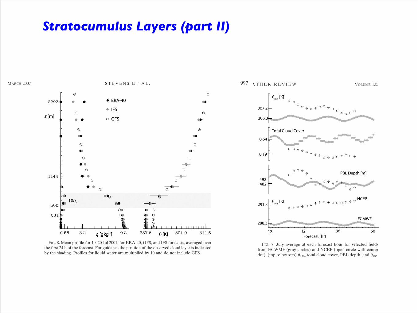
Moreover, despite the shortcomings of the IFS, its rep-resentation of PBL clouds is clearly superior to that ofthe GFS. These results provide further evidence that,overall, the IFS-based ERA-40 represents the structureof the lower troposphere near 30°N, 120°W during July2001 better than the earlier-generation GFS-basedNCEP product.

Figure 8 illustrates the vertical structure of ! and qfrom ERA-40, IFS, and GFS for the period 10–20 July.In addition to more pointedly illustrating the warm biasof the GFS, and a slight tendency of the GFS PBL to beless well mixed in terms of specific humidity, these pro-files show that while each of the products qualitativelycapture the gross structure of a shallow marine layer,the transition between the PBL and the free tropo-sphere takes place over too deep a layer. This transitionlayer, which is several hundreds of meters in depth inthe models, is much sharper in the data: temperaturesincrease 10 K or more, while ozone, chemical constitu-ents, and water vapor often fall to background values,in tens of meters or less (Stevens et al. 2003a). Al-though some smearing of the mean interface can beexpected because of spatial and temporal variability inthe PBL depth, during the 10 days over which data wasaveraged to construct Fig. 8 the ERA-40 PBL depth

averaged 600 m with a standard deviation of 88 m.Thus, the thickness of the transition layer is unlikely tobe a result of great temporal variability in the depth ofa PBL topped at any given time by a much sharperinterface, but rather due to an inability of the modelphysics and numerics to maintain such a sharp inter-face. Telling in this respect is the structure of the cloudfield. It is placed at about the right altitude by both thereanalysis and the forecast systems, but because themodels produce a much shallower mixed layer, this cor-responds to a level more centered in the model inver-sion, rather than at the top of the STBL as is the casefor the data. Moreover, the cloud field has significantlyless liquid water. At any given grid point the liquidwater specific humidity never exceeds 0.1 g kg"1 in the10-day IFS record, which is more than an order of mag-nitude less than expected. As a result the structure ofthe mean profiles is more reminiscent of shallow cumu-liform convection than it is of stratocumulus convec-tion.

5. A routine July?The above analysis gives an idea of the large-scale

variability and STBL structure for one particular July.It also gives an indication of the skill with which differ-

FIG. 8. Mean profile for 10–20 Jul 2001, for ERA-40, GFS, and IFS forecasts, averaged overthe first 24 h of the forecast. For guidance the position of the observed cloud layer is indicatedby the shading. Profiles for liquid water are multiplied by 10 and do not include GFS.

MARCH 2007 S T E V E N S E T A L . 997

to argue that this is simply a problem of insufficientvertical resolution.

In summary, boundary layer depths inferred fromISCCP cloud-top temperatures and TMI SSTs matchthe observed boundary layer depths remarkably well.Estimates of L from ISCCP optical depths also repre-sent the observed cloud liquid water path as well asestimates derived from microwave-based retrievals.NNRA does not provide estimates of either zi or L.Both quantities are underestimated in ERA-40.

d. Inferences from forecast models

Here we evaluate the ECMWF IFS and NCEP GFSusing the DYCOMS-II data. Doing so gives further in-sight into the ability of the models underlying the re-analyses to represent the structure of the lower tropo-sphere in the study region. This is particularly true forERA-40, which was produced using the same version ofthe IFS as was being used to generate forecasts in Julyof 2001 (Uppala et al. 2005). Because ERA-40 incor-porated the dropsondes from the field program, such acomparison also allows us to evaluate how the IFS be-haved in the absence of the dropsonde data. In the caseof NCEP, an analysis of the GFS data allows us toexamine a product on spatial scales more commensu-rate with the study region. This analysis also providesan opportunity to investigate NCEP’s representation ofthe PBL depth and cloud cover, neither of which wereavailable as reanalysis products.

Table 3 lists the value of state variables from the IFSand GFS forecasts averaged between 0000 UTC andhour 24, and between hour 24 and hour 48, for everyday of July 2001, as well as averages for all of July fromERA-40 and NNRA. For identical initial data and sta-tionary statistics, a perfect model should yield identicalrepresentations of the mean state among these threerepresentations, each corresponding to the observed

state. From the table it is apparent that the IFS is quiteconsistent with its reanalysis product (ERA-40), withthe only significant trend being an increase in the zonalwinds later in the forecasts. From this we conclude thatthe fidelity of the ERA-40 time-mean products is un-likely to be a result of the incorporation of special data.The same conclusion cannot be drawn for NNRA, aswithin the PBL the GFS develops a large (3 K) warmand modest dry bias almost from the start. The warmbias increases through the forecast period. A similarbias is evident in comparisons of the structure of thestratocumulus-topped boundary layer as representedby the GFS and as observed during the East PacificInvestigation of Climate (EPIC; Bretherton et al.2004b, their Fig. 10), suggesting that this is not a re-gional effect. The GFS and IFS predict PBL depths thatlook more similar to each other than to the data.

July averages of ! near 850 hPa, total cloud cover,PBL depth, and ! near 993 hPa are plotted versus fore-cast hour in Fig. 7. The different start times reflect theinitialization at 1200 UTC on the previous day for the72-h IFS forecasts as compared with the 0000 UTC ini-tialization for the 48-h GFS forecasts. In addition toillustrating the mean state biases noted above (e.g., !993

from the GFS), Fig. 7 indicates that the GFS has largertemporal trends and a markedly weaker diurnal cycle.

TABLE 3. Reanalysis and forecast averages for July 2001. Here! is averaged on model levels, thus !850 is actually valid on modellevels 49 and 32 for IFS and GFS, respectively, which correspondto average pressures of 860 and 846 hPa. Likewise, !m is averagedon model levels 56 and 40 for IFS and GFS, respectively. On theselevels, both models average a mean pressure of 993 hPa.

Field ERA-40

IFS

NNRA

GFS

0–24 24–48 00–24 24–48

!850 (K) 306.9 306.0 306.0 308.1 307.6 307.0q850 (g kg"1) 3.8 3.9 3.5 4.1 3.7 3.5!m (K) 288.2 288.5 288.3 288.0 291.6 292.4qm (g kg"1) 9.6 9.7 9.7 9.8 9.1 9.2um (m s"1) 2.1 3.3 3.5 3.8 3.5 3.7#m (m s"1) "6.1 "6.3 "6.4 "5.7 "6.2 "5.8zi (m) 460 480 480 — 510 480

FIG. 7. July average at each forecast hour for selected fieldsfrom ECWMF (gray circles) and NCEP (open circle with centerdot): (top to bottom) !850, total cloud cover, PBL depth, and !993.

996 M O N T H L Y W E A T H E R R E V I E W VOLUME 135

Cumulus-Topped Layers

surface heat and moisture fluxes

radiative driving warm, dry, subsiding free-troposphere

zi

entrainment

ql (averaged over cloud) 2310

765

qf (z) s

f (z)

297.3 307.1 311.9 0.9 2.9 13.65 0 0.22

ql,adiabatic cumulus mass flux

transition layer

sea surface

• Thermal and momentum boundary layer are increasingly distinct.

• The concept of a mass flux, M

Cumulus-Topped Layer (Part II)

1876 VOLUME 58J O U R N A L O F T H E A T M O S P H E R I C S C I E N C E S

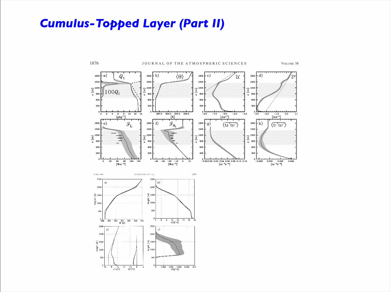
FIG. 3. Mean profiles averaged over analysis period and displayed following format of previous figure. Thin solid lines delineate initialstate. Plotted, clockwise from top left are (a) total-water Qt and liquid water Ql mixing ratios, (b) potential temperature !, (c) zonal windU, (d) meridional wind V, (e) total-water mixing ratio flux FL, (f ) liquid water potential temperature flux (g) zonal momentum flux, andF ,"l

(h) meridional momentum flux. All the fluxes are the sum of the resolved and SGS fluxes. (e) and (f ) The mass-flux estimate of the flux isalso shown by the short horizontal lines at five heights [see section 4b(1) for details]. (a) The thin dashed line denotes Q s in the cloud layer.

successful in representing a regime with intermediatecloud fractions, although actual values of cloud fraction(and the ensuing domain-averaged liquid water path)varied sharply across the simulations. Albrecht (1991)shows time series of cloud fraction from both the R/VPlanet and the R/VMeteor. Over the R/V Planet,whosethermodynamic environment was most commensuratewith the specified initial data, cloud fractions variedbetween 0.1 and 0.9, with a distinct diurnal cycle anda trend toward lower cloud fractions as the ship driftedover warmer water. Thus while the simulations arebroadly consistent with the data, the intercomparisonclearly illustrates the difficulty of using LES to quantifyrelationships between cloud fraction and the large-scaleenvironment—at least in this regime.

b. Mean profiles and fluxes

With the exception of the velocity deficits (i.e., u #ug, $ # $ g) in the subcloud (and to a lesser extent) cloudlayer, the evolution of the simulations over 8 h resultsin remarkably small changes in the mean state (Fig. 3).This is largely a result of the forcings balancing withinthe Eulerian domain. The thermodynamic fluxes in Fig.3 illustrate the tight coupling of the cloud and subcloudlayers. To the extent that the boundary layer is consid-ered as a single layer, energetically coupled to the sur-face on short timescales, the PBL in this regime extendsfrom the surface to the base of the trade inversion (whichwe denote by zi) at 1500 m.On the other hand, both the momentum profiles and

fluxes behave distinctly in the cloud versus the subcloudlayers. The largest velocity deficits (i.e., departures ofthe velocities from their geostrophic values) occur inthe subcloud layer (i.e., for z % h, where h denotes theheight of the subcloud layer) and a weak zonal jet de-velops just above z & h. Above this jet (Fig. 3c), zonalvelocity gradients reverse, taking on the sign of thegradients of the geostrophic wind. However, the zonalmomentum flux (Fig. 3g) does not change sign, whichimplies a weak countergradient transport of zonal mo-mentum. This locally countergradient flux is consistentwith momentum being mixed out of the subcloud layer,as opposed to down the local gradient. The meridionalwind (Fig. 3d) has a markedly different structure, tend-ing to peak near the surface with relatively more activemomentum transport (Fig. 3h) in the cloud. The greatertransport of meridional momentum in the cloud layer isconsistent with the somewhat larger differences betweenthe meridional wind (as compared to the zonal wind)in the subcloud versus the cloud layer.The aforementioned variability in cloud statistics is

most evident at cloud top, where both cloud water andcloud fraction (shown later) have global maxima thatvary widely. Flow visualization and conditional sam-pling (also discussed below) indicate that the variabilityin cloud water largely reflects different predictions ofthe lifetime (and hence extent) of stratiform detrainmentregions associated with cumulus clouds impinging uponthe trade inversion. The mean state saturation deficit(i.e., s # t) is a minimum at about 1400 m, just belowq qthe region of maximum liquid water. The tendency for

15 MAY 2003 1205S I E B E S M A E T A L .

FIG. 3. Mean profiles averaged over the last hour of (a) potential temperature !, (b) water vapor specific humidity q" , (c) the horizontalvelocity components, and (d) the liquid water ql. The solid lines indicate the average and the band is a width of twice the standard deviationof the participating models. The dashed lines indicate the initial profiles.

erated from a single LES code using different initialrandom seeds all suggested that an averaging time of T# 3 h was necessary to produce reliable statistics ofhigher-order statistics. Given that the first 3 h of thesimulation were influenced by the spinup features de-scribed earlier, subsequent presentations of time-aver-aged results represent averages over the final 3 h of thesimulations.

1) FLUXES AND VARIANCES

Figure 4 shows the results for the time-averaged tur-bulent fluxes of the conserved variables andw$! $!

, as well as the buoyancy flux and the liquidw$q$ w$! $t "

water flux . The buoyancy flux is defined with re-w$q$!

spect to the virtual potential temperature !" # !(1 %0.61q" & ql).The profiles can be subdivided in two regions:w$q$t

between the surface up to near the inversion at 1500 m,the fluxes are only marginally decreasing with height.This is followed by a strong decrease in the inversionwhere most of the moisture surface flux is deposited.More specifically, about 2/3 of surface flux is usedw$q$tto moisten the inversion, whereas the remaining 1/3 isdeposited in the cloud layer and the subcloud layer. Allmodels except the Regional Atmospheric Modeling Sys-tem (RAMS) model show this behavior. The RAMSmodel showed considerably more temporal variabilityfor all fields than the other models and 3 h is probablynot a long enough averaging time for this model.

Remarks

• Boundary layers are rich in processes.

• Boundary layers are thin.

• Boundary layers are turbulent.

Some words about modeling

• Similarity.

• Local rules: (L, z, q, S, N).

• Bulk rules (h, ∆T, ∆U, ∆F, D, M, B).

• Forgotten parameters (∆x, ∆z).

• Stochastic Methods.

• Hybrid approaches.

• Two scale models.

Similarity

! = " (g/h)1/2

Non-dimensional equivalence

!u/!z = α (u*/z)

The law of the wall (log-layer) -- intermediate asympototic

!u/!z = α (u*/z) f(")

Local vs Bulk Rules

• Fluxes proportional to local TKE, e.

• Mixing profile scales with bulk quantities.

• The length scales are the trick in both approaches.

!te = !u"w"!zu + w"b" ! "

K =!

e!

K(z) = v"hg(") where " = z/h

versus

K =!

e!

K(z) = v"hg(") where " = z/h

In practice both often combine elements of the other.

Summary

• Boundary layers are essential.

• Most ideas are built around classical concepts.

• Our task is difficult because boundary layers are rich, thin and turbulent.

• Many essential problems remain.

• Fine-scale modeling is helping to enrich the phenomenological basis for our modeling.