Embed Size (px)
Citation preview
arX
iv:m
ath/
0608
422v
4 [
mat
h.PR
] 1
9 Ja
n 20
09
Boundary Partitions in Trees and Dimers
Richard W. Kenyon∗ David B. Wilson†
Abstract
Given a finite planar graph, a grove is a spanning forest in which every componenttree contains one or more of a specified set of vertices (called nodes) on the outerface. For the uniform measure on groves, we compute the probabilities of the differentpossible node connections in a grove. These probabilities only depend on boundarymeasurements of the graph and not on the actual graph structure, i.e., the probabilitiescan be expressed as functions of the pairwise electrical resistances between the nodes,or equivalently, as functions of the Dirichlet-to-Neumann operator (or response matrix)on the nodes. These formulae can be likened to generalizations (for spanning forests)of Cardy’s percolation crossing probabilities, and generalize Kirchhoff’s formula forthe electrical resistance. Remarkably, when appropriately normalized, the connectionprobabilities are in fact integer-coefficient polynomials in the matrix entries, where thecoefficients have a natural algebraic interpretation and can be computed combinato-rially. A similar phenomenon holds in the so-called double-dimer model: connectionprobabilities of boundary nodes are polynomial functions of certain boundary measure-ments, and as formal polynomials, they are specializations of the grove polynomials.Upon taking scaling limits, we show that the double-dimer connection probabilitiescoincide with those of the contour lines in the Gaussian free field with certain naturalboundary conditions. These results have direct application to connection probabilitiesfor multiple-strand SLE2, SLE8, and SLE4.
1 Introduction
1.1 Grove partitions
A circular planar graph G is a finite weighted planar graph with a set of vertices N on itsouter face numbered 1, . . . , n in counterclockwise order. The vertices in N are called nodes,and the remaining vertices are called inner vertices. Define a grove to be a spanningacyclic subgraph (a forest) of G such that each component tree contains at least one node.The weight of a grove is the product of the weights of the edges it contains. We studyrandom groves where the probability of a grove is proportional to its weight.
The term grove comes from Carroll and Speyer [CS04] and Petersen and Speyer [PS05]who studied a special case of (our) groves, with a particular family of underlying graphs.Since we are dealing with a natural generalization we chose to keep their terminology, and
2000 Mathematics Subject Classification. 60C05, 82B20, 05C05, 05C50.Key words and phrases. Tree, grove, double-dimer model, Gaussian free-field, Dirichlet-to-Neumann
matrix, meander, SLE.∗University of British Columbia, Vancouver, BC V6T 1Z2, Canada†Microsoft Research, Redmond, WA 98052, USA
1

Boundary partitions in trees and dimers Kenyon & Wilson 2
refer to the special case they discuss as Carroll-Speyer groves, which we will discuss furtherin a subsequent paper [KW08].
The connected components of a grove partition the nodes into a planar (i.e. noncrossing)partition. For example, when n = 4, there are 14 planar partitions: 1234, 1|234, 2|134,3|124, 4|123, 12|34, 23|14, 1|2|34, 1|3|24, 1|4|23, 2|3|14, 2|4|13, 3|4|12, 1|2|3|4. There are nogroves with the partition 13|24 because it is not planar (there is no way to connect nodes 1and 3 and nodes 2 and 4 by disjoint paths within a circular planar graph). For general n,the number of noncrossing partitions is the nth Catalan number Cn = (2n)!/(n!(n+1)!) (see[Sta99, ex. 6.19(pp), pg. 226]).
1 2 3
4
567
8
12
3
4
56
7
8
Figure 1: A random grove (left) of a rectangular grid with 8 nodes on the outer face. Inthis grove there are 4 trees (each colored differently), and the partition of the nodes is{{1}, {2, 7, 8}, {3, 4, 5}, {6}}, which we write as 1|278|345|6, and illustrate schematically asshown on the right.
If σ is a planar partition of 1, . . . , n, we let Pr(σ) denote the probability that a randomgrove of G partitions the nodes according to σ. Since groves with one component are trees,we refer to the partition σ = 123 . . . n as the tree partition. When there are n nodes wecall the partition σ = 1|2|3| · · · |n the uncrossing, since groves with this partition typecontain no crossings (i.e. paths) connecting the nodes. We show how to compute for eachplanar partition σ the probability Pr(σ) of it occurring in a random grove, as a functionof the electrical properties of the graph G, when G is viewed as a resistor network withconductances equal to the edge weights.
We let Ri,j denote the effective electrical resistance between nodes i and j, i.e., thevoltage at node i which, when node j is held at 0 volts, causes a unit current to flow throughthe circuit from node i to node j. (A good reference for basic electric circuit theory is[DS84].) Let Li,j denote the current that would flow into node j if node i were set to onevolt and the remaining nodes set to zero volts. Though it is not obvious from this definition,Li,j = Lj,i (see Appendix A). The Li,j are the negatives of the entries of the “responsematrix” (Dirichlet-to-Neumann matrix) of (G,N), on which we provide further backgroundin Appendix A, see also [CdV98]. We prove
Boundary partitions in trees and dimers Kenyon & Wilson 3
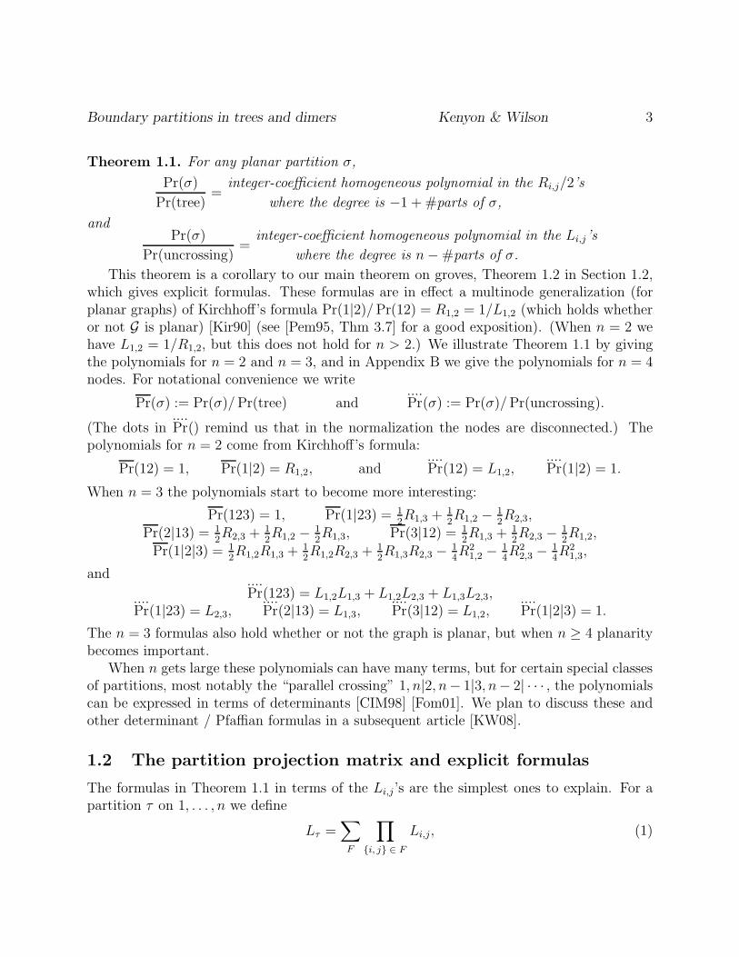
Theorem 1.1. For any planar partition σ,
Pr(σ)
Pr(tree)=
integer-coefficient homogeneous polynomial in the Ri,j/2’s
where the degree is −1 + #parts of σ,
andPr(σ)
Pr(uncrossing)=
integer-coefficient homogeneous polynomial in the Li,j’s
where the degree is n − #parts of σ.
This theorem is a corollary to our main theorem on groves, Theorem 1.2 in Section 1.2,which gives explicit formulas. These formulas are in effect a multinode generalization (forplanar graphs) of Kirchhoff’s formula Pr(1|2)/ Pr(12) = R1,2 = 1/L1,2 (which holds whetheror not G is planar) [Kir90] (see [Pem95, Thm 3.7] for a good exposition). (When n = 2 wehave L1,2 = 1/R1,2, but this does not hold for n > 2.) We illustrate Theorem 1.1 by givingthe polynomials for n = 2 and n = 3, and in Appendix B we give the polynomials for n = 4nodes. For notational convenience we write
Pr(σ) := Pr(σ)/ Pr(tree) and....Pr(σ) := Pr(σ)/ Pr(uncrossing).
(The dots in....Pr() remind us that in the normalization the nodes are disconnected.) The
polynomials for n = 2 come from Kirchhoff’s formula:
Pr(12) = 1, Pr(1|2) = R1,2, and....Pr(12) = L1,2,
....Pr(1|2) = 1.
When n = 3 the polynomials start to become more interesting:
Pr(123) = 1, Pr(1|23) = 12R1,3 + 1
2R1,2 − 1
2R2,3,
Pr(2|13) = 12R2,3 + 1
2R1,2 − 1
2R1,3, Pr(3|12) = 1
2R1,3 + 1
2R2,3 − 1
2R1,2,
Pr(1|2|3) = 12R1,2R1,3 + 1
2R1,2R2,3 + 1
2R1,3R2,3 − 1
4R2
1,2 − 14R2
2,3 − 14R2
1,3,
and....Pr(123) = L1,2L1,3 + L1,2L2,3 + L1,3L2,3,....
Pr(1|23) = L2,3,....Pr(2|13) = L1,3,
....Pr(3|12) = L1,2,
....Pr(1|2|3) = 1.
The n = 3 formulas also hold whether or not the graph is planar, but when n ≥ 4 planaritybecomes important.
When n gets large these polynomials can have many terms, but for certain special classesof partitions, most notably the “parallel crossing” 1, n|2, n− 1|3, n− 2| · · · , the polynomialscan be expressed in terms of determinants [CIM98] [Fom01]. We plan to discuss these andother determinant / Pfaffian formulas in a subsequent article [KW08].
1.2 The partition projection matrix and explicit formulas
The formulas in Theorem 1.1 in terms of the Li,j ’s are the simplest ones to explain. For apartition τ on 1, . . . , n we define
Lτ =∑
F
∏
{i, j} ∈ F
Li,j, (1)
Boundary partitions in trees and dimers Kenyon & Wilson 4
where the sum is over those spanning forests F of the complete graph on n vertices 1, . . . , nfor which trees of F span the parts of τ , and the product is over edges {i, j} of forest F .
This definition makes sense whether or not the partition τ is planar. For example, L1|234 =L2,3L3,4 + L2,3L2,4 + L2,4L3,4 and L13|24 = L1,3L2,4. As we shall see, the “L polynomials” ofTheorem 1.1 are in fact integer linear combinations of the Lτ ’s:
Pr(σ)
Pr(1|2| · · · |n)=∑
τ
P(t)σ,τLτ .
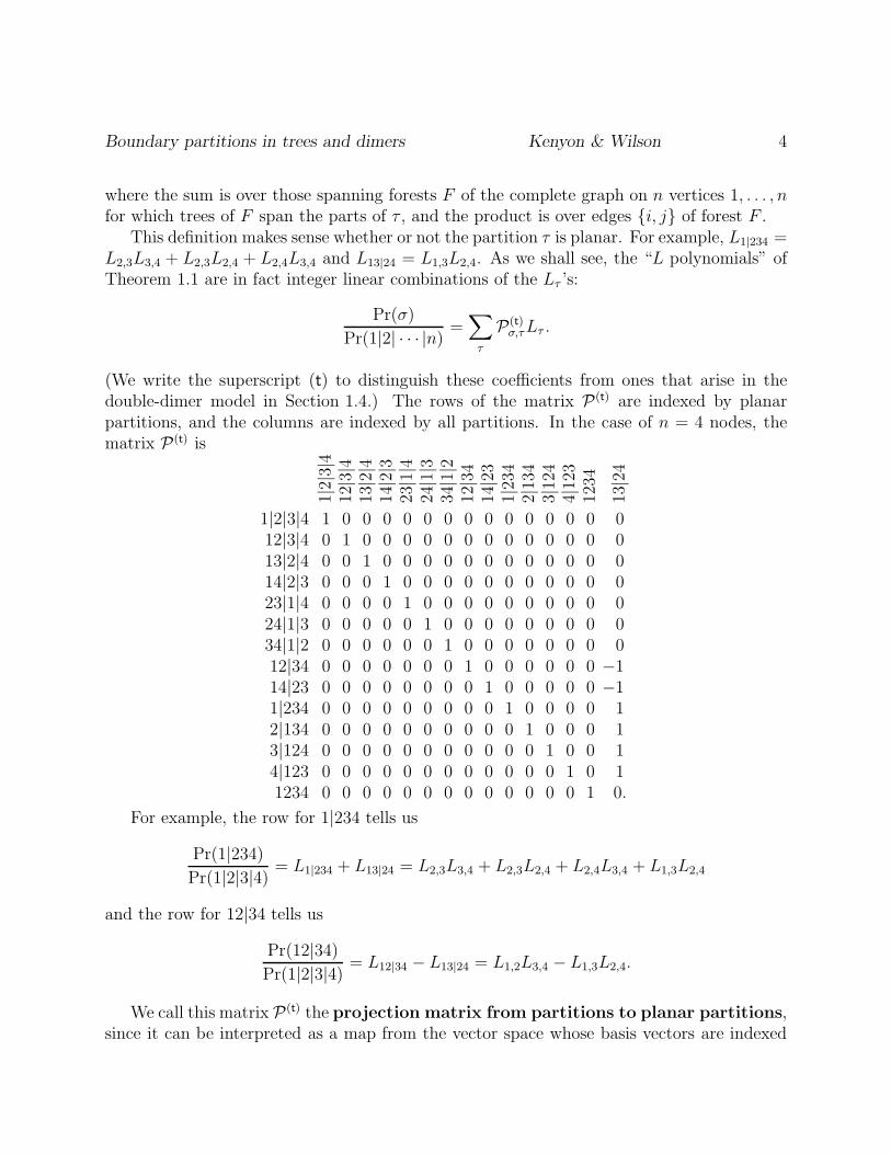
(We write the superscript (t) to distinguish these coefficients from ones that arise in thedouble-dimer model in Section 1.4.) The rows of the matrix P(t) are indexed by planarpartitions, and the columns are indexed by all partitions. In the case of n = 4 nodes, thematrix P(t) is
1|2|
3|4
12|3|4
13|2|4
14|2|3
23|1|4
24|1|3
34|1|2
12|3
414|2
31|
234
2|13
43|
124
4|12
312
34
13|2
4
1|2|3|4 1 0 0 0 0 0 0 0 0 0 0 0 0 0 012|3|4 0 1 0 0 0 0 0 0 0 0 0 0 0 0 013|2|4 0 0 1 0 0 0 0 0 0 0 0 0 0 0 014|2|3 0 0 0 1 0 0 0 0 0 0 0 0 0 0 023|1|4 0 0 0 0 1 0 0 0 0 0 0 0 0 0 024|1|3 0 0 0 0 0 1 0 0 0 0 0 0 0 0 034|1|2 0 0 0 0 0 0 1 0 0 0 0 0 0 0 012|34 0 0 0 0 0 0 0 1 0 0 0 0 0 0 −114|23 0 0 0 0 0 0 0 0 1 0 0 0 0 0 −11|234 0 0 0 0 0 0 0 0 0 1 0 0 0 0 12|134 0 0 0 0 0 0 0 0 0 0 1 0 0 0 13|124 0 0 0 0 0 0 0 0 0 0 0 1 0 0 14|123 0 0 0 0 0 0 0 0 0 0 0 0 1 0 11234 0 0 0 0 0 0 0 0 0 0 0 0 0 1 0.
For example, the row for 1|234 tells us
Pr(1|234)
Pr(1|2|3|4)= L1|234 + L13|24 = L2,3L3,4 + L2,3L2,4 + L2,4L3,4 + L1,3L2,4
and the row for 12|34 tells us
Pr(12|34)
Pr(1|2|3|4)= L12|34 − L13|24 = L1,2L3,4 − L1,3L2,4.
We call this matrix P(t) the projection matrix from partitions to planar partitions,since it can be interpreted as a map from the vector space whose basis vectors are indexed

Boundary partitions in trees and dimers Kenyon & Wilson 5
by all partitions to the vector space whose basis vectors are indexed by planar partitions,and the map is the identity on planar partitions. For example, the column for 13|24 tells us
13|24 projects to − 12|34 − 14|23 + 1|234 + 2|134 + 3|124 + 4|123.
(We could have written the right-hand-side as −e12|34 − e14|23 + e1|234 + e2|134 + e3|124 + e4|123,where the e’s are basis vectors, but it is convenient to suppress the vector notation andinstead write formal linear combinations of partitions.)
The projection matrix may be computed using some simple combinatorial transforma-tions of partitions. Given a partition τ , the τ th column of P(t) may be computed by repeatedapplication of the following transformation rule, until the resulting formal linear combinationof partitions only involves planar partitions. The rule generalizes the transformation
1
23
4 1
23
4 1
23
4 1
23
4 1
23
4 1
23
4 1
23
4
++++−−→
13|24 → −12|34 − 14|23 + 1|234 + 2|134 + 3|124 + 4|123
(which is derived in Lemma 2.3) to partitions τ containing additional items and parts. Ifpartition τ is nonplanar, then there will exist items a < b < c < d such that a and c belongto one part, and b and d belong to another part. Arbitrarily subdivide the part containinga and c into two sets A and C such that a ∈ A and c ∈ C, and similarly subdivide the partcontaining b and d into B ∋ b and D ∋ d. Let the remaining parts of partition τ (if any) bedenoted by “rest.” Then the transformation rule is
AC|BD| rest → A|BCD| rest + B|ACD| rest + C|ABD| rest + D|ABC| rest− AB|CD| rest −AD|BC| rest . (Rule 1)
In Section 2 we prove
Theorem 1.2. Any partition τ may be transformed into a formal linear combination ofplanar partitions by repeated application of Rule 1, and the resulting linear combination doesnot depend on the choices made when applying Rule 1, so that we may write
τ →∑
planar partitions σ
P(t)σ,τσ.
For any planar partition σ, these same coefficients P(t)σ,τ satisfy the equation
Pr(σ)
Pr(1|2| · · · |n)=
∑
partitions τ
P(t)σ,τLτ
for circular planar graphs. More generally, for any graph these coefficients satisfy∑
partitions τ
P(t)σ,τ
Pr(τ)
Pr(1|2| · · · |n)=
∑
partitions τ
P(t)σ,τLτ .
(The last equation specializes to the previous one because P(t)σ,σ = 1, for planar τ 6= σ we
have P(t)σ,τ = 0, and for nonplanar τ we have Pr(τ) = 0 for circular planar graphs.)
Boundary partitions in trees and dimers Kenyon & Wilson 6
1.3 Double-dimer pairings
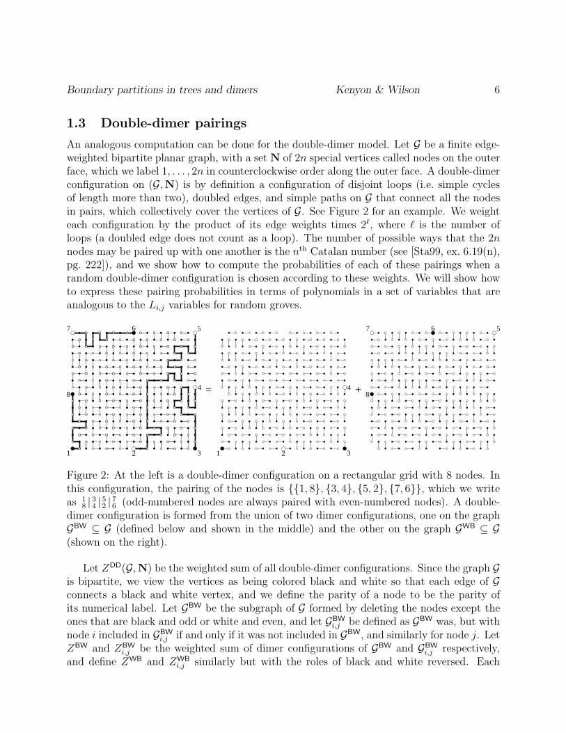
An analogous computation can be done for the double-dimer model. Let G be a finite edge-weighted bipartite planar graph, with a set N of 2n special vertices called nodes on the outerface, which we label 1, . . . , 2n in counterclockwise order along the outer face. A double-dimerconfiguration on (G,N) is by definition a configuration of disjoint loops (i.e. simple cyclesof length more than two), doubled edges, and simple paths on G that connect all the nodesin pairs, which collectively cover the vertices of G. See Figure 2 for an example. We weighteach configuration by the product of its edge weights times 2ℓ, where ℓ is the number ofloops (a doubled edge does not count as a loop). The number of possible ways that the 2nnodes may be paired up with one another is the nth Catalan number (see [Sta99, ex. 6.19(n),pg. 222]), and we show how to compute the probabilities of each of these pairings when arandom double-dimer configuration is chosen according to these weights. We will show howto express these pairing probabilities in terms of polynomials in a set of variables that areanalogous to the Li,j variables for random groves.
1 2 3
4
567
8
1 2 3
4
567
8= +
Figure 2: At the left is a double-dimer configuration on a rectangular grid with 8 nodes. Inthis configuration, the pairing of the nodes is {{1, 8}, {3, 4}, {5, 2}, {7, 6}}, which we writeas 1
8 | 34 | 52 | 76 (odd-numbered nodes are always paired with even-numbered nodes). A double-dimer configuration is formed from the union of two dimer configurations, one on the graphGBW ⊆ G (defined below and shown in the middle) and the other on the graph GWB ⊆ G(shown on the right).
Let ZDD(G,N) be the weighted sum of all double-dimer configurations. Since the graph Gis bipartite, we view the vertices as being colored black and white so that each edge of Gconnects a black and white vertex, and we define the parity of a node to be the parity ofits numerical label. Let GBW be the subgraph of G formed by deleting the nodes except theones that are black and odd or white and even, and let GBW
i,j be defined as GBW was, but withnode i included in GBW
i,j if and only if it was not included in GBW, and similarly for node j. LetZBW and ZBW
i,j be the weighted sum of dimer configurations of GBW and GBW
i,j respectively,and define ZWB and ZWB
i,j similarly but with the roles of black and white reversed. Each
Boundary partitions in trees and dimers Kenyon & Wilson 7
of these quantities can be computed via determinants, see [Kas67] and Section 3. It turnsout that ZDD = ZBWZWB; this is essentially Ciucu’s graph factorization theorem [Ciu97,Thm. 1.2] (except that in the factorization theorem, any edges that connect two nodes arereweighted by 1/2, and here they are not), see Section 3. (The two dimer configurations inFigure 2 are on the graphs GBW and GWB.) The variables that play the role of Li,j in grovesare defined by
Xi,j = ZBW
i,j /ZBW.
For each planar matching of the nodes σ, let Pr(σ) be the probability that a randomdouble-dimer configuration has this set of connections. In Section 3 we prove
Theorem 1.3. For any planar pairing σ on 2n nodes,
Pr(σ)ZWB
ZBW= integer-coefficient homogeneous polynomial of degree n in the quantities Xi,j.
This theorem is a corollary to our main theorem on double-dimer pairings, Theorem 1.4in Section 1.4, which gives the polynomials explicitly. To illustrate this theorem, we give afew examples. For notational simplicity let us define
Pr(σ) = Pr(σ)ZWB/ZBW.
In the simplest nontrivial case there are 2n = 4 nodes, and two possible planar pairings,{{1, 2}, {3, 4}} and {{1, 4}, {2, 3}}, which we write as 1
2 | 34 and 1
4 | 32 . Their normalized
probabilities are
Pr( 12 | 34 ) = X1,2X3,4 Pr( 1
4 | 32 ) = X1,4X2,3.
These above two formulas are essentially equivalent to a formula of Kuo [Kuo04, Thms 2.1and 2.3]. In the case of 2n = 6 nodes, we have
Pr( 12 | 36 | 54 ) =X3,6(X1,2X4,5 − X1,4X2,5)
Pr( 12 | 34 | 56) =X1,4X2,5X3,6 + X1,2X3,4X5,6
and similarly for cyclic permutations of the indices. These cover the five possibilities.In the case of 2n = 8 nodes, we have
Pr( 12 | 38 | 56 | 74 ) =(X1,2X7,4 − X1,4X7,2)(X3,8X5,6 − X5,8X3,6)
= − det
X1,2 X1,4 0 00 0 X3,6 X3,8
0 0 X5,6 X5,8
X7,2 X7,4 0 0
Pr( 12 | 34 | 56 | 78 ) =X1,2X3,4X5,6X7,8 + X1,4X3,8X5,6X7,2 + X1,6X3,4X5,8X7,2+
X1,6X3,8X5,2X7,4 + X1,2X3,6X5,8X7,4 + X1,4X3,6X5,2X7,8 − 2X1,4X3,6X5,8X7,2

Boundary partitions in trees and dimers Kenyon & Wilson 8
Pr( 12 | 38 | 54 | 76 ) = det
X1,2 X1,4 X1,6 00 0 X3,6 X3,8
X5,2 X5,4 0 X5,8
X7,2 X7,4 X7,6 0
and similarly for cyclic permutations of the indices. These cover the fourteen possibilities.As can be seen from the way we have written these polynomials, for some pairings they
are expressible as determinants. We plan to discuss such formulas further in [KW08].Of course we could also express the pairing probabilities in terms of the variables X∗
i,j =ZWB
i,j /ZWB. The polynomials are exactly the same, although the underlying variables repre-sent different quantities.
1.4 The odd-even pairing projection matrix and explicit formulas
The explicit computation of the double-dimer pairing probability formulas is quite analogousto the computation of the grove partition probability formulas. The role of the Lτ variablesfor groves is replaced by variables that are indexed by the n! pairings between the odd nodesand the even nodes (“odd-even pairings”). If τ is such an odd-even pairing, then we define
Xτ = X(τ) =∏
i odd
Xi,τ(i)
and it turns out to be more convenient to work with
X ′τ = X ′(τ) = (−1)#crosses in τ
∏
i odd
Xi,τ(i)
where a cross in a pairing τ is a set of four nodes a < b < c < d such that a and c are pairedwith one another and b and d are paired with one another. The “X polynomials” are in factinteger linear combinations of the X ′
τ ’s:
Pr(σ) =∑
odd-even pairings τ
P(DD)σ,τ X ′
τ .
As with grove partitions, we construct a projection matrix, but with double-dimer pair-ings the matrix projects a vector space with basis vectors indexed by odd-even pairings toa vector space whose basis vectors are indexed by planar pairings. Recall that for grovesthe projection matrix P(t) has dimensions Cn ×Bn, the nth Catalan number by the nth Bellnumber; for double-dimers the projection matrix P(DD) has dimensions Cn×n!. When n = 4the projection matrix P(DD) is

Boundary partitions in trees and dimers Kenyon & Wilson 9
1 2|3 4|5 6|7 8
1 2|3 4|5 8|7 6
1 2|3 6|5 4|7 8
1 2|3 8|5 4|7 6
1 2|3 8|5 6|7 4
1 4|3 2|5 6|7 8
1 4|3 2|5 8|7 6
1 6|3 2|5 4|7 8
1 6|3 4|5 2|7 8
1 8|3 2|5 4|7 6
1 8|3 2|5 6|7 4
1 8|3 4|5 2|7 6
1 8|3 4|5 6|7 2
1 8|3 6|5 4|7 2
1 2|3 6|5 8|7 4
1 4|3 6|5 2|7 8
1 4|3 8|5 2|7 6
1 4|3 8|5 6|7 2
1 6|3 2|5 8|7 4
1 6|3 4|5 8|7 2
1 6|3 8|5 4|7 2
1 8|3 6|5 2|7 4
1 4|3 6|5 8|7 2
1 6|3 8|5 2|7 4
12 | 34 | 56 | 78 1 0 0 0 0 0 0 0 0 0 0 0 0 0 −1 −1 0 −1 0 −1 0 0 −2 112 | 34 | 58 | 76 0 1 0 0 0 0 0 0 0 0 0 0 0 0 1 0 −1 0 0 1 0 0 1 −112 | 36 | 54 | 78 0 0 1 0 0 0 0 0 0 0 0 0 0 0 1 1 0 0 0 0 −1 0 1 −112 | 38 | 54 | 76 0 0 0 1 0 0 0 0 0 0 0 0 0 0 −1 0 1 0 0 0 1 0 −1 112 | 38 | 56 | 74 0 0 0 0 1 0 0 0 0 0 0 0 0 0 1 0 0 1 0 0 0 0 1 014 | 32 | 56 | 78 0 0 0 0 0 1 0 0 0 0 0 0 0 0 0 1 0 1 −1 0 0 0 1 −114 | 32 | 58 | 76 0 0 0 0 0 0 1 0 0 0 0 0 0 0 0 0 1 0 1 0 0 0 0 116 | 32 | 54 | 78 0 0 0 0 0 0 0 1 0 0 0 0 0 0 0 −1 0 0 1 0 1 0 −1 116 | 34 | 52 | 78 0 0 0 0 0 0 0 0 1 0 0 0 0 0 0 1 0 0 0 1 0 0 1 018 | 32 | 54 | 76 0 0 0 0 0 0 0 0 0 1 0 0 0 0 0 0 −1 0 −1 0 −1 −1 1 −218 | 32 | 56 | 74 0 0 0 0 0 0 0 0 0 0 1 0 0 0 0 0 0 −1 1 0 0 1 −1 118 | 34 | 52 | 76 0 0 0 0 0 0 0 0 0 0 0 1 0 0 0 0 1 0 0 −1 0 1 −1 118 | 34 | 56 | 72 0 0 0 0 0 0 0 0 0 0 0 0 1 0 0 0 0 1 0 1 0 −1 1 −118 | 36 | 54 | 72 0 0 0 0 0 0 0 0 0 0 0 0 0 1 0 0 0 0 0 0 1 1 0 1
We call this matrix P(DD) the projection matrix from odd-even pairings to planar
pairings.For example, the first row tells us that
Pr( 12 | 34 | 56 | 78 ) = X ′( 1
2 | 34 | 56 | 78 ) − X ′( 12 | 36 | 58 | 74 ) − X ′( 1
4 | 36 | 52 | 78 ) − X ′( 14 | 38 | 56 | 72 )
− X ′( 16 | 34 | 58 | 72 ) − 2X ′( 1
4 | 36 | 58 | 72 ) + X ′( 16 | 38 | 52 | 74 )
= X1,2X3,4X5,6X7,8 + X1,2X3,6X5,8X7,4 + X1,4X3,6X5,2X7,8 + X1,4X3,8X5,6X7,2
+ X1,6X3,4X5,8X7,2 − 2X1,4X3,6X5,8X7,2 + X1,6X3,8X5,2X7,4.
As with the matrix P(t), we may compute the τ th column of the matrix P(DD) via asequence of simple combinatorial transformations on the odd-even pairings. The prototypicalexample of the transformation rule is
1
23
4
56
1
23
4
56
1
23
4
56
1
23
4
56
1
23
4
56
1
23
4
56
++ −−→
14 | 36 | 52 → 1
4 | 32 | 56 + 12 | 36 | 54 + 1
6 | 34 | 52 − 12 | 34 | 56 − 1
6 | 32 | 54(which is derived in Lemma 3.7). Compare with the 16th column, column 1
4 | 36 | 5
2 | 78 , in the
above matrix. More generally, suppose that n ≥ 3 and the odd-even pairing is a1
b1| a2
b2| · · · |an
bn,
Boundary partitions in trees and dimers Kenyon & Wilson 10
where the ai’s are odd and the bi’s are even. Then the transformation rule is
a1
b1| a2
b2| a3
b3| rest → a1
b2| a2
b1| a3
b3| rest + a1
b1| a2
b3| a3
b2| rest + a1
b3| a2
b2| a3
b1| rest
− a1
b2| a2
b3| a3
b1| rest− a1
b3| a2
b1| a3
b2| rest (Rule 2)
where in the above “rest” represents a4
b4| · · · |an
bnwith unchanged pairings.
For example, when transforming 14 | 36 | 58 | 72 we can hold the pair {7, 2} fixed:
14 | 36 | 58 | 72 → 1
6 | 34 | 58 | 72 + 14 | 38 | 56 | 72 + 1
8 | 36 | 54 | 72 − 16 | 38 | 54 | 72 − 1
8 | 34 | 56 | 72.
Of these odd-even pairings, the third and fifth ones are planar, but the others require ad-ditional applications of Rule 2. When transforming the first of these terms, if we hold thepair {3, 4} fixed,
16 | 34 | 58 | 72 → 1
8 | 34 | 56 | 72 + 16 | 34 | 52 | 78 + 1
2 | 34 | 58 | 76 − 18 | 34 | 52 | 76 − 1
2 | 34 | 56 | 78 ,
then the resulting odd-even pairings are all planar. The other terms above may be similarlytransformed into linear combinations of planar pairings, and when they are added up, theresult is summarized in column 1
4 | 36 | 58 | 72 of the projection matrix P(DD).In Section 3 we prove
Theorem 1.4. Any odd-even pairing τ may be transformed into a formal linear combinationof planar pairings by repeated application of Rule 2, and the resulting linear combination doesnot depend on the choices made when applying Rule 2, so that we may write
τ →∑
planar pairings σ
P(DD)σ,τ σ.
For any planar pairing σ, these same coefficients P(DD)σ,τ satisfy the equation
Pr(σ)ZWB
ZBW=
∑
odd-even pairings τ
P(DD)σ,τ X ′(τ)
for bipartite circular planar graphs.
In Section 4 we show that the P(DD) projection matrix of order n is up to signs embeddedin the P(t) projection matrix of order 2n:
Theorem 1.5.
P(DD)σ,τ = (−1)σ−1τP(t)
σ,τ
where on the left σ and τ denote odd-even pairings, and on the right they are interpretedas partitions consisting of parts of size 2, and in the sign they are interpreted as maps fromodd nodes to even nodes, so that σ−1τ is a permutation on odd nodes, and (−1)σ−1τ is itssignature.
Boundary partitions in trees and dimers Kenyon & Wilson 11
1.5 Multichordal SLE connection probabilities
In Section 5 we consider the connection probabilities in the scaling limits of the spanningtree and double-dimer models, and also of the contour lines in the scaling limit of the discreteGaussian free field with certain boundary conditions.
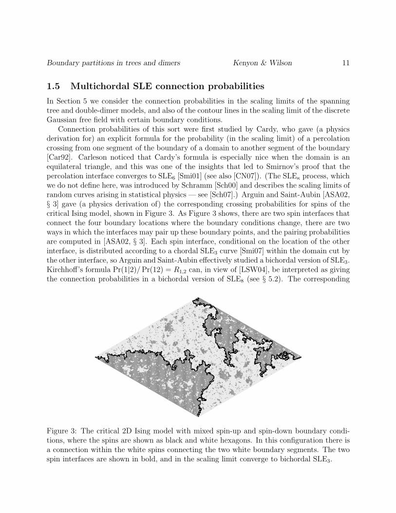
Connection probabilities of this sort were first studied by Cardy, who gave (a physicsderivation for) an explicit formula for the probability (in the scaling limit) of a percolationcrossing from one segment of the boundary of a domain to another segment of the boundary[Car92]. Carleson noticed that Cardy’s formula is especially nice when the domain is anequilateral triangle, and this was one of the insights that led to Smirnov’s proof that thepercolation interface converges to SLE6 [Smi01] (see also [CN07]). (The SLEκ process, whichwe do not define here, was introduced by Schramm [Sch00] and describes the scaling limits ofrandom curves arising in statistical physics — see [Sch07].) Arguin and Saint-Aubin [ASA02,§ 3] gave (a physics derivation of) the corresponding crossing probabilities for spins of thecritical Ising model, shown in Figure 3. As Figure 3 shows, there are two spin interfaces thatconnect the four boundary locations where the boundary conditions change, there are twoways in which the interfaces may pair up these boundary points, and the pairing probabilitiesare computed in [ASA02, § 3]. Each spin interface, conditional on the location of the otherinterface, is distributed according to a chordal SLE3 curve [Smi07] within the domain cut bythe other interface, so Arguin and Saint-Aubin effectively studied a bichordal version of SLE3.Kirchhoff’s formula Pr(1|2)/ Pr(12) = R1,2 can, in view of [LSW04], be interpreted as givingthe connection probabilities in a bichordal version of SLE8 (see § 5.2). The corresponding
Figure 3: The critical 2D Ising model with mixed spin-up and spin-down boundary condi-tions, where the spins are shown as black and white hexagons. In this configuration there isa connection within the white spins connecting the two white boundary segments. The twospin interfaces are shown in bold, and in the scaling limit converge to bichordal SLE3.
Boundary partitions in trees and dimers Kenyon & Wilson 12
connection probabilities for other values of κ were given in [BBK05, § 8.2 and 8.3] (see also[Dub06, § 4.1]).
In a related vein, there has been much study of the physics of multiple-strand networks ofself-avoiding walks (polymers), loop-erased random walks, and other random paths that areeither known or believed to be related to SLEκ. For example, the “watermelon exponents”describe the scaling behavior of the partition function when multiple strands meet at a pointin the interior or on the boundary of a domain [Sal86, DS87, Dup92, Dup87]. The boundarywatermelon exponents for L strands can be extracted from the limiting behavior of theconnection probabilities of L strands of (multichordal) SLE connecting 2L boundary pointswhen L of the boundary points are close to each other and the other L boundary points areclose to each other, though of course these connection probabilities contain more informationthan is summarized in the exponents. This approach does not yield the bulk watermelonexponents, since to obtain the bulk exponents one would need the endpoints of the strandsto be in the interior of the domain. The scaling exponents associated with more complicatedmultiple-strand networks (for 2 ≤ κ ≤ 8) have also been derived [Dup87, Dup89, OB88]. See[Dup06] for up-to-date lecture notes on the physics of networks of polymers and other typesof strands and their relation to SLE.
It is only natural to consider the connection probabilities of multichordal SLEκ, whichis defined in [KL07], and has the property that, conditional on one curve, the remainingcurves are distributed according to multichordal SLEκ with fewer curves within the domaincut by the conditioned curve. Kozdron and Lawler [KL07] studied multichordal SLEκ fora fixed connection topology (when κ ≤ 4). Cardy exhibited several discrete models withmultiple interfaces that arise naturally in the context of conformal field theory, for whichthe interfaces have the same joint distribution (whose scaling limit is thought to be multi-chordal SLE) conditional on a particular connection topology, but for which the connectiontopologies have different probabilities [Car07]. (Thus to discuss connection topology proba-bilities of multichordal SLE, one must specify a discrete model whose scaling limit is beingtaken.) Comparing two such models, the connection topology probabilities in one modelhave different weights compared to another such model, but these weights do not dependon the domain or on the location of the boundary points where the boundary conditionschange, so that the set of all connection topology probabilities in one such model determinesthe connection topology probabilities in another such model. Dubedat [Dub06] analyzed thegeneral multichordal SLEκ connection probabilities (and included special discussion of thecases κ = 2, 6, 8), but there still remain open problems regarding these connection probabil-ities when the number of curves is large.
The scaling limit calculations in Section 5 yield explicit formulas for the multichordalSLEκ connection probabilities in the cases κ = 2, 4, 8 (for any number of curves, for anyconnection topology). There is a scaling limit relation [LSW04] between branches of uniformspanning trees on periodic planar graphs and SLE2. Essentially, the scaling limit, as thelattice spacing tends to zero, of a branch of the uniform spanning tree on a bounded domain,tends to a random simple curve which is equal in law to SLE2. Similarly, the curve whichwinds between the uniform spanning tree and its dual spanning tree (Figure 9) converges
Boundary partitions in trees and dimers Kenyon & Wilson 13
in the scaling limit to an SLE8 [LSW04]. The double-dimer paths are thought to have ascaling limit that is given by SLE4, but this has not been proved. However, the contourlines in the discrete Gaussian free field with certain boundary conditions have been provedto converge to SLE4 [SS06] in the scaling limit, and using the results of [SS06] we prove inTheorem 5.1 that the probability distribution of the pairings of these contour lines coincideswith the pairing distribution for the double-dimer model.
2 Grove partitions
2.1 The meander matrix
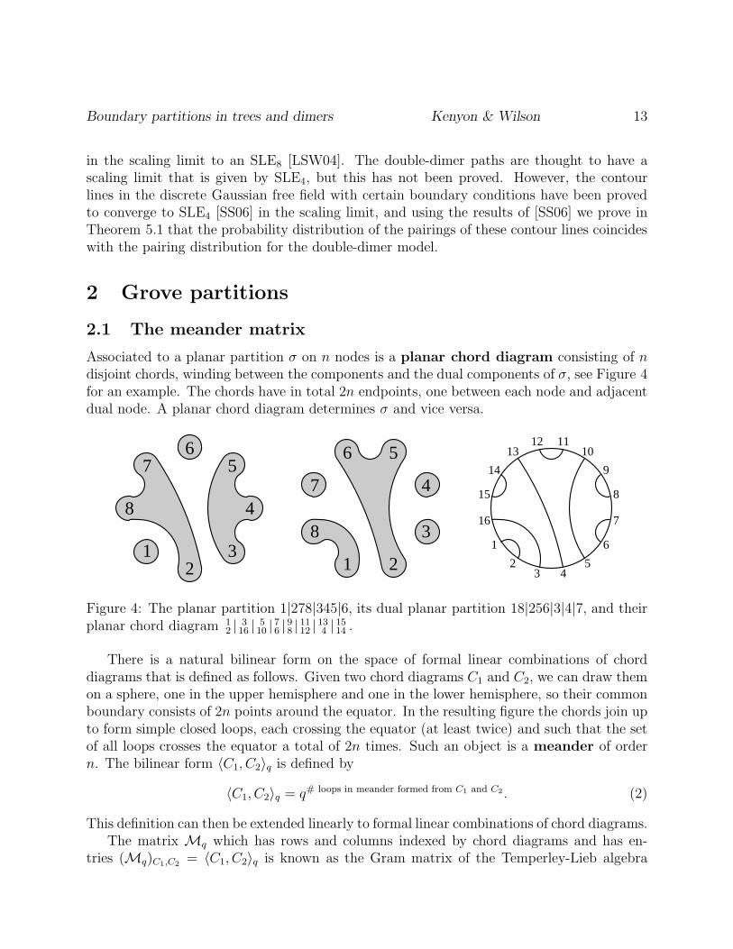
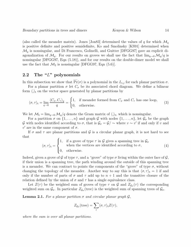
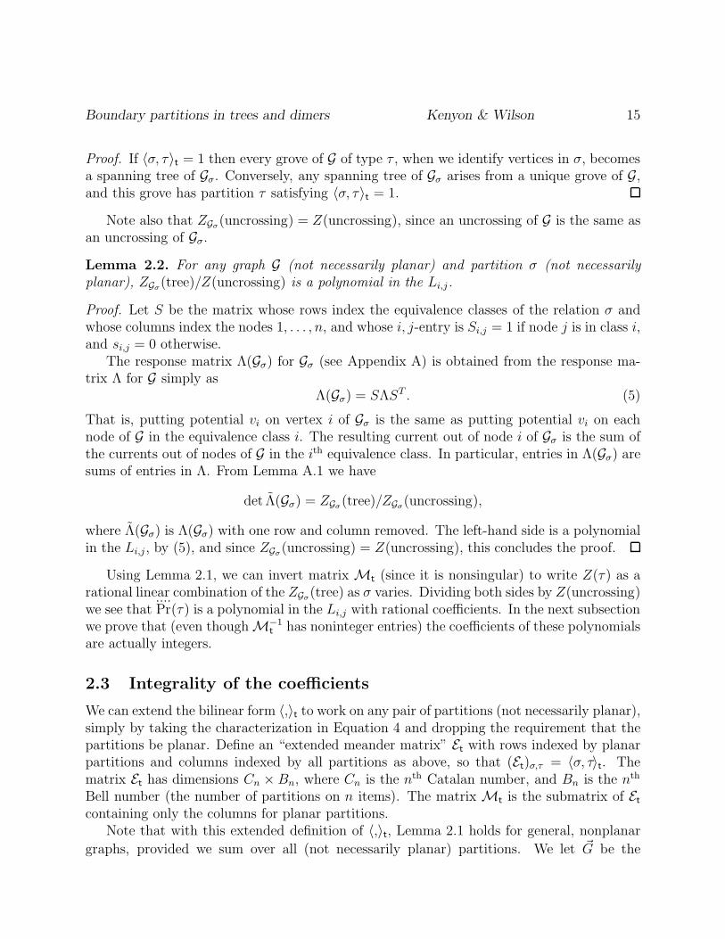
Associated to a planar partition σ on n nodes is a planar chord diagram consisting of ndisjoint chords, winding between the components and the dual components of σ, see Figure 4for an example. The chords have in total 2n endpoints, one between each node and adjacentdual node. A planar chord diagram determines σ and vice versa.
12
3
4
56
7
8
1 2
3
4
56
7
81
23 4
5
6
7
8
9
101112
13
14
15
16
Figure 4: The planar partition 1|278|345|6, its dual planar partition 18|256|3|4|7, and theirplanar chord diagram 1
2 | 316 | 5
10 | 76 | 98 | 1112 | 134 | 1514 .
There is a natural bilinear form on the space of formal linear combinations of chorddiagrams that is defined as follows. Given two chord diagrams C1 and C2, we can draw themon a sphere, one in the upper hemisphere and one in the lower hemisphere, so their commonboundary consists of 2n points around the equator. In the resulting figure the chords join upto form simple closed loops, each crossing the equator (at least twice) and such that the setof all loops crosses the equator a total of 2n times. Such an object is a meander of ordern. The bilinear form 〈C1, C2〉q is defined by
〈C1, C2〉q = q# loops in meander formed from C1 and C2 . (2)
This definition can then be extended linearly to formal linear combinations of chord diagrams.The matrix Mq which has rows and columns indexed by chord diagrams and has en-
tries (Mq)C1,C2= 〈C1, C2〉q is known as the Gram matrix of the Temperley-Lieb algebra
Boundary partitions in trees and dimers Kenyon & Wilson 14
(also called the meander matrix). Jones [Jon83] determined the values of q for which Mq
is positive definite and positive semidefinite, Ko and Smolinsky [KS91] determined whenMq is nonsingular, and Di Francesco, Golinelli, and Guitter [DFGG97] gave an explicit di-agonalization of Mq. For our results on groves we shall use the fact that limq→0 Mq/q isnonsingular [DFGG97, Eqn (5.18)], and for our results on the double-dimer model we shalluse the fact that M2 is nonsingular [DFGG97, Eqn (5.6)].
2.2 The “L” polynomials
In this subsection we show that....Pr(σ) is a polynomial in the Li,j for each planar partition σ.
For a planar partition σ let Cσ be its associated chord diagram. We define a bilinearform 〈,〉t on the vector space generated by planar partitions by
〈σ, τ〉t = limq→0
〈Cσ, Cτ 〉qq
=
{1, if meander formed from Cσ and Cτ has one loop,
0, otherwise.(3)
We let Mt = limq→0 Mq/q denote the Gram matrix of 〈,〉t, which is nonsingular.For a partition σ on {1, . . . , n} and graph G with nodes {1, . . . , n}, let Gσ be the graph
G with nodes identified according to σ, that is Gσ = G/ ∼ where v ∼ v′ if and only if v andv′ are in the same component of σ.
If σ and τ are planar partitions and G is a circular planar graph, it is not hard to seethat
〈σ, τ〉t =
1, if a grove of type τ in G gives a spanning tree in Gσ
when the vertices are identified according to σ,
0, otherwise.
(4)
Indeed, given a grove of G of type τ , and a “grove” of type σ living within the outer face of G,if their union is a spanning tree, the path winding around the outside of this spanning treeis a meander. We can contract to points the components of the “grove” of type σ, withoutchanging the topology of the meander. Another way to say this is that 〈σ, τ〉t = 1 if andonly if the number of parts of σ and τ add up to n + 1 and the transitive closure of therelation defined by the union of σ and τ has a single equivalence class.
Let Z(τ) be the weighted sum of groves of type τ on G and ZGσ(τ) the correspondingweighted sum on Gσ. In particular ZGσ(tree) is the weighted sum of spanning trees of Gσ.
Lemma 2.1. For a planar partition σ and circular planar graph G,
ZGσ(tree) =∑
τ
〈σ, τ〉tZ(τ),
where the sum is over all planar partitions.
Boundary partitions in trees and dimers Kenyon & Wilson 15
Proof. If 〈σ, τ〉t = 1 then every grove of G of type τ , when we identify vertices in σ, becomesa spanning tree of Gσ. Conversely, any spanning tree of Gσ arises from a unique grove of G,and this grove has partition τ satisfying 〈σ, τ〉t = 1.
Note also that ZGσ(uncrossing) = Z(uncrossing), since an uncrossing of G is the same asan uncrossing of Gσ.
Lemma 2.2. For any graph G (not necessarily planar) and partition σ (not necessarilyplanar), ZGσ(tree)/Z(uncrossing) is a polynomial in the Li,j.
Proof. Let S be the matrix whose rows index the equivalence classes of the relation σ andwhose columns index the nodes 1, . . . , n, and whose i, j-entry is Si,j = 1 if node j is in class i,and si,j = 0 otherwise.
The response matrix Λ(Gσ) for Gσ (see Appendix A) is obtained from the response ma-trix Λ for G simply as
Λ(Gσ) = SΛST . (5)
That is, putting potential vi on vertex i of Gσ is the same as putting potential vi on eachnode of G in the equivalence class i. The resulting current out of node i of Gσ is the sum ofthe currents out of nodes of G in the ith equivalence class. In particular, entries in Λ(Gσ) aresums of entries in Λ. From Lemma A.1 we have
det Λ(Gσ) = ZGσ(tree)/ZGσ(uncrossing),
where Λ(Gσ) is Λ(Gσ) with one row and column removed. The left-hand side is a polynomialin the Li,j , by (5), and since ZGσ(uncrossing) = Z(uncrossing), this concludes the proof.
Using Lemma 2.1, we can invert matrix Mt (since it is nonsingular) to write Z(τ) as arational linear combination of the ZGσ(tree) as σ varies. Dividing both sides by Z(uncrossing)we see that
....Pr(τ) is a polynomial in the Li,j with rational coefficients. In the next subsection
we prove that (even though M−1t has noninteger entries) the coefficients of these polynomials
are actually integers.
2.3 Integrality of the coefficients
We can extend the bilinear form 〈,〉t to work on any pair of partitions (not necessarily planar),simply by taking the characterization in Equation 4 and dropping the requirement that thepartitions be planar. Define an “extended meander matrix” Et with rows indexed by planarpartitions and columns indexed by all partitions as above, so that (Et)σ,τ = 〈σ, τ〉t. Thematrix Et has dimensions Cn × Bn, where Cn is the nth Catalan number, and Bn is the nth
Bell number (the number of partitions on n items). The matrix Mt is the submatrix of Et
containing only the columns for planar partitions.Note that with this extended definition of 〈,〉t, Lemma 2.1 holds for general, nonplanar
graphs, provided we sum over all (not necessarily planar) partitions. We let ~G be the
Boundary partitions in trees and dimers Kenyon & Wilson 16
column vector of “glue variables”, whose entries are ~Gσ = ZGσ(tree) for σ a planar partition
of 1, . . . , n. Let ~Z be the column vector of partition variables, whose entries are ~Zτ = Z(τ)where τ runs over all partitions. The extension of Lemma 2.1 to the nonplanar setting gives
~G = Et~Z. (6)
For any not necessarily planar graph G on n nodes there is an electrically equivalentcomplete graph K on n vertices (in which every vertex is a node): it is the graph whoseedge {i, j} has conductance Li,j(G,N). (The graphs G and K are electrically equivalent inthe sense that, when the same voltages are applied to the nodes of G and K, the currentresponses will be the same, i.e., they have the same Dirichlet-to-Neumann matrix.) Notethat each ZK(τ) is trivially a polynomial in the Li,j, since each crossing of K has weight whichis a monomial in the Li,j. In fact, we can write this polynomial explicitly: for each part λ ofτ , we count the weighted sum of spanning trees of the complete graph on the vertices in λ,and then take the product over the different parts of τ . Recalling our definition of Lτ inEquation 1, we have that ZK(τ) = Lτ . For example
ZK(1|23|456) = 1 · L2,3 · (L4,5L5,6 + L4,5L4,6 + L4,6L5,6) = L1|23|456.
We let ~L be the column vector of partition variables for K: ~Lτ = ZK(τ) = Lτ .
By the preceding equation, for the graph K, Equation 6 specializes to ~G = Et~L. By
Lemma 2.2, for any graph, ~G is determined by the L’s, so we have
~G = Et~Z = Et
~L
for any graph. For planar graphs, the entries of ~Z corresponding to nonplanar partitions are0, so Et
~Z = Mt~Z, and hence Mt
~Z = Et~L. Since Mt is invertible,
~Z = M−1tEt
~L.
We defineP(t) = M−1
tEt.
We shall see how to compute P(t) directly, i.e. without inverting Mt. The direct computationof P(t) involves only integer operations, from which it will follow that the “L polynomials”have integer coefficients.
What is the matrix P(t)? For each planar partition σ, the row σ tells us Zσ =∑
τ P(t)σ,τLτ .
For each partition τ , the τ th column gives us a linear combination of planar partitions∑σ P
(t)σ,τσ that is equivalent to τ in the sense that for any planar partition ρ,
⟨ρ,∑
σ
P(t)σ,τσ
⟩
t
=∑
σ
P(t)σ,τ (Mt)ρ,σ = (MtP(t))ρ,τ = (Et)ρ,τ = 〈ρ, τ〉t.
Boundary partitions in trees and dimers Kenyon & Wilson 17
(We shall see that⟨ρ,∑
σ P(t)σ,τσ
⟩
t
= 〈ρ, τ〉t for nonplanar partitions ρ too.)
Let us say that two linear combinations of partitions on n items∑
τ αττ and∑
τ βττ
are equivalent (t≡) if for any (possibly nonplanar) partition ρ on n items
∑τ ατ 〈ρ, τ〉t =∑
τ βτ 〈ρ, τ〉t. For example,
Lemma 2.3. 1|234 + 2|134 + 3|124 + 4|123t≡ 12|34 + 13|24 + 14|23
Proof. For any partition ρ with three parts, 〈ρ, LHS〉t = 2 = 〈ρ, RHS〉t: By symmetryconsiderations, we need only consider one such parition, say 12|3|4, and
〈12|3|4, LHS〉t = 1 + 1 + 0 + 0 = 0 + 1 + 1 = 〈12|3|4, RHS〉t.
For partitions ρ with other numbers of parts, 〈ρ, LHS〉t = 0 = 〈ρ, RHS〉t, since fromEquation 4 〈ρ, τ〉t = 0 whenever #{parts of ρ} + #{parts of τ} 6= #items + 1.
As we shall see, this lemma, together with the following two lemmas, which show howto adjoin new parts and new items to the partitions of the left- and right-hand sides of an
equivalence (t≡), will allow us to write any partition as an equivalent (
t≡) sum of planarpartitions.
Lemma 2.4. Suppose n ≥ 2, τ is a partition of 1, . . . , n − 1, and τt≡∑
σ ασσ. Then
τ |n t≡∑
σ
ασσ|n.
Proof. If {n} is a part of ρ then 〈ρ, τ |n〉t = 0 = 〈ρ, RHS〉t. Otherwise 〈ρ, τ |n〉t = 〈ρrn, τ〉t =∑σ ασ〈ρ r n, σ〉t =
∑σ ασ〈ρ, σ|n〉t.
If τ is a partition of 1, . . . , n− 1 and j ∈ {1, . . . , n− 1}, we can insert a new item n intothe part of τ that contains item j. We refer to the resulting partition on 1, . . . , n as “τ withn inserted into j’s part.”
Lemma 2.5. Suppose n ≥ 2, τ is a partition of 1, . . . , n − 1, j ∈ {1, . . . , n − 1}, and
τt≡∑
σ ασσ. Then
[τ with n inserted into j’s part]t≡∑
σ
ασ[σ with n inserted into j’s part].
Proof. If j and n are in the same part of partition ρ, as well as being in the same partof partition π, then by (4) 〈ρ, π〉t = 0. Thus 〈ρ, [τ with n inserted into j’s part]〉t = 0 =〈ρ, RHS〉t. If j and n are in separate parts of ρ, then let ρ′ denote the partition obtainedfrom ρ by merging the two parts containing j and n, and then deleting n. By (4) we have
〈ρ, [τ with n inserted into j’s part]〉t = 〈ρ′, τ〉t =∑
σ
ασ〈ρ′, σ〉t = 〈ρ, RHS〉t.

Boundary partitions in trees and dimers Kenyon & Wilson 18
Lemmas 2.3, 2.4, and 2.5 imply that the left-hand-side and right-hand-side of transfor-
mation Rule 1 are equivalent (t≡).
Theorem 2.6. For any partition τ , there is an equivalent (t≡) integer linear combination of
planar partitions∑
σ ασσ (i.e., where each ασ ∈ Z).
Proof. We prove this by induction on the number of items in the partition. The theorem istrue for n ≤ 3 since each such partition τ is already planar (and with Lemma 2.3, we see thatit is also true for n = 4). Suppose τ contains more items. If {n} is a part of τ , then we mayuse the induction hypothesis together with Lemma 2.4 to find the desired linear combinationof planar partitions. Otherwise, item n is in the same part as some other item j (if thereis more than one choice of j, it does not matter which one we pick). By the induction
hypothesis, we may write τ rnt≡ an integer linear combination of planar partitions, and by
Lemma 2.5, we may write τ as an integer linear combination of “almost planar” partitions,by which we mean partitions that would be planar if the item n were deleted from them.
Next we use Lemmas 2.3, 2.4, 2.5 to express an almost-planar partition µ as an equivalentinteger linear combination of planar partitions. We shall use induction on the number k ofparts of µ that cross the chord from j to n. There is nothing to show if k = 0, andotherwise we consider the part S of µ closest to j that crosses the chord from j to n.We let a = {i ∈ S : i < j} and c = {i ∈ S : i > j}, both of which are nonempty,b = the part of µ containing j, and d = {n}. Let a0 ∈ a and c0 ∈ c. From Lemma 2.3, uponrelabeling 1 → a0, 2 → j, 3 → c0, and 4 → n, we get
a0, c0|j, nt≡ a0|j, c0, n + j|a0, c0, n + c0|a0, j, n + n|a0, j, c0 − a0, j|c0, n − a0, n|j, c0.
Using Lemma 2.5 we may insert the rest of a into the parts containing a0, the rest of c intothe parts containing c0, and the rest of b into the parts containing j, to obtain
a ∪ c|b ∪ dt≡ a|b ∪ c ∪ d + b|a ∪ c ∪ d + c|a ∪ b ∪ d + d|a ∪ b ∪ c − a ∪ b|c ∪ d − a ∪ d|b ∪ c.
By further application of Lemmas 2.4 and 2.5, we may adjoin each of the remaining parts ofµ to the left-hand-side (thereby obtaining µ) and to each partition on the right-hand-side.Of the resulting partitions on the right-hand-side, the fourth one is planar, and the otherpartitions are almost planar with k − 1 parts crossing the chords from n to the rest of n’spart.
For a partition τ , let∑
σ ασσ be any linear combination of planar partitions equivalent
(t≡) to τ . Now
∑σ(P
(t)σ,τ − ασ)σ lies in the null-space of Mt, but Mt is nonsingular, so
P(t)σ,τ = ασ for each σ. In particular, the linear combination promised by Theorem 2.6 is
unique, and gives the τ th column of P(t). This linear combination was obtained by repeatedapplication of Rule 1, which completes the proof of Theorem 1.2, which in turn implies thesecond part of Theorem 1.1 as a corollary.
We remark that the entries of the matrix P(t) are all 0 or ±1 for n ≤ 7 nodes, but thatwhen n ≥ 8 other integers appear.
Boundary partitions in trees and dimers Kenyon & Wilson 19
2.4 The “R” polynomials
In this subsection we prove the first part of Theorem 1.1, i.e., we show that Pr(σ) is acertain polynomial in the Ri,j ’s for each planar partition σ. We start with some elementarycharacterizations of the Ri,j and Li,j variables in terms of groves.
Proposition 2.7. The resistance between i and j is
Ri,j =∑
A:i∈A,j∈Ac
Pr(A|Ac).
Proof. If nodes i and j were the only two nodes, then we know from Kirchhoff’s formula (thecase n = 2) that Ri,j is the ratio of the probability that i and j are in different componentsof a 2-component random grove, to the probability of a 1-component grove. When thereare other nodes, these 2-component groves necessarily take the form A|Ac where i ∈ A andj ∈ Ac. (See the top half of Figure 6.)
The following proposition may be derived from Lemma 4.1 of [CIM98], but for the reader’sconvenience we provide a short proof.
Proposition 2.8. For i 6= j,
Li,j =....Pr(i, j|rest singletons),
i.e., Li,j =....Pr(σ) where σ is the partition in which every part is a singleton except for the
part {i, j}.Proof. Recall from the construction in Theorem 2.6, that whenever a partition τ is expressedas an equivalent sum of planar partitions, each of the partitions has the same number of partsas τ . Since σ has n − 1 parts, and any partition τ with n − 1 parts is already planar, theσth row of P(t) is nonzero only in the σth column, so
....Pr(σ) = ~Lσ = Li,j.
Any circular planar graph G has a dual circular planar graph G∗, as shown in Figure 5.The dual G∗ has an inner vertex for every bounded face of G, and a node numbered i betweenconsecutive nodes i, i + 1 mod n of G. For each edge of G there is a dual edge of G∗, whoseconductance is, by definition, the reciprocal of the conductance on the corresponding edgeof G. For each grove of G there is a dual grove of G∗ formed from the duals of the edges ofG not contained in the grove (see Figure 5). A grove in G has weight equal to the weight ofits dual grove in G∗, times the product of the conductances of all edges in G.
Proposition 2.9. For the dual graph we have
L∗i,j = 1
2Ri,j + 1
2Ri+1,j+1 − 1
2Ri,j+1 − 1
2Ri+1,j (7)
andR∗
i,j =∑ ∑
1≤i′<j′≤nchord i′, j′ crosses dual chord i, j
Li′,j′. (8)
Boundary partitions in trees and dimers Kenyon & Wilson 20
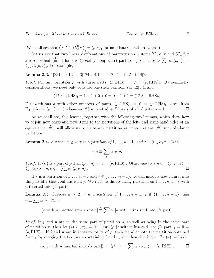
Figure 5: Shown here is a circular planar graph G with four nodes (shown in black) andone inner vertex, with edges shown as solid lines. The dual circular planar graph G∗ hasfour nodes (shown in white) and two inner vertices, with edges shown as dashed lines. Alsoshown is a grove of G of type 1|234 (the edges of the grove are shown in bold) and its dualgrove of G∗ (with edges also shown in bold), which has type 14|2|3.
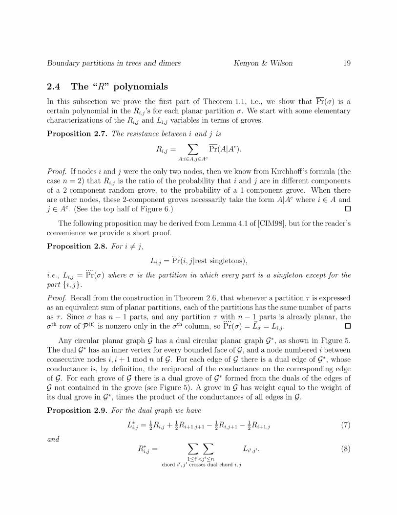
Proof. By Proposition 2.7, R∗i,j =
∑A:i∈A,j∈Ac Pr
∗(A|Ac). But dual nodes i and j are in
opposite parts of A|Ac if and only if the partition dual to A|Ac is i′, j′|rest singleton for somechord i′, j′ crossing dual chord i, j (see Figure 6); applying Proposition 2.8 then yields (8).Expanding the right-hand-side of (7) using (8) yields the left-hand-side of (7).
111111
111111222222
333333
444444
444444
555555
111111222222
333333
444444555555
Figure 6: R1,4 can be expressed as a sum of 2-part partitions in which 1 and 4 are in differentparts. For the dual resistance R∗
1,4 in the dual graph, the sum over dual partitions becomes asum over partitions consisting of a doubleton part and rest singletons, where the doubletonpart separates dual nodes 1 and 4.

Boundary partitions in trees and dimers Kenyon & Wilson 21
Proof of first part of Theorem 1.1. Since the dual of a partition σ is a partition σ∗ on thedual graph, and each grove has the same weight as its dual grove, times a constant, we have
Pr(σ)
Pr(tree)=
Pr(σ∗)
Pr(dual uncrossing),
which by the second part of Theorem 1.1 is an integer-coefficient polynomial in the L∗i,j’s,
which by Proposition 2.9 is an integer-coefficient polynomial in the Ri,j/2’s.
3 Double-dimer pairings
Recall that for our double-dimer results we assume the circular planar graph G is bipartite,so we may color its vertices black and white so that each edge connects a black vertex toa white vertex. It is convenient to assume that the nodes on the outer face alternate incolor, so that the odd-numbered nodes are black and the even-numbered nodes are white.If the graph G does not satisfy this property, we can extend G by adjoining an extra vertexand edge with weight 1 for each node that has the wrong color (refer to Figure 7), and thedouble-dimer configurations of the extended graph are in one-to-one weight-preserving andconnection-preserving correspondence with the double-dimer configurations of the original
1 2 3
4
567
8
1 2 3
4
567
8
Figure 7: Double-dimer configuration on a rectangular grid with 8 terminal nodes. In thisconfiguration the pairing of the nodes is {{1, 8}, {3, 4}, {5, 2}, {7, 6}}, which we write as18 | 3
4 | 52 | 7
6 . The double-dimer configurations on the graph on the left are in one-to-onecorrespondence with the double-dimer configurations of the extended graph on the right, forwhich the odd terminals are colored black and the even terminals are colored white.

Boundary partitions in trees and dimers Kenyon & Wilson 22
graph. Furthermore, the quantities ZWB, ZBW as well as the variables Xi,j are the same onthis new graph as they were on G. Henceforth we assume without loss of generality that thenode colors of G alternate between black and white.
3.1 Polynomiality
Since the nodes alternate in color, ZBW is the weighted sum of dimer covers of G. Recall thatZDD is the weighted sum of double-dimer covers of (G,N) where each of the terminal nodesis included in only one of the dimer coverings. Let S be a balanced subset of nodes, that is,a subset containing an equal number k of white and black nodes. Let ZD(S) = ZD(G \ S)be the weighted sum of dimer covers of G \ S, and ZD = ZD(∅) = ZBW. The superpositionof a dimer cover of G \ S and a dimer cover of G \ Sc, where Sc = N \ S, is a double-dimercover of (G,N). In fact, we have
Lemma 3.1. ZD(S)ZD(Sc) is a sum of double-dimer configurations for all connection topolo-gies π for which π connects no element of S to an element of Sc. That is,
ZD(S)ZD(Sc) = ZDD∑
π
MS,π Pr(π), (9)
where MS,π is 0 or 1 according to whether π connects nodes in S to Sc or not.
As a special case, when S = ∅ we have ZD(∅)ZD(N) = ZDD, which is closely relatedto Ciucu’s graph factorization theorem [Ciu97, Thm. 1.2]. Ciucu showed how to enumeratedimer coverings in a bipartite graph with bilateral symmetry. Dimer coverings of the wholegraph correspond to double-dimer configurations of one half of the graph, with vertices onthe symmetry axis corresponding to nodes, except that there is an extra factor of 2 in weightfor each path connecting a pair of nodes, unless the path consists of a single edge. So thegraph factorization theorem contains a power of 2 for each pair of nodes, and a weight of 1/2for each edge on the symmetry axis, neither of which appear in Lemma 3.1.
Our remaining double-dimer results only make sense if there are double-dimer configu-rations of G, which implies that there are dimer configurations of G, so that G has equalnumbers of black and white vertices. After proving this lemma, we shall henceforth makethis assumption.
Proof of Lemma 3.1. Each double-dimer path connecting a pair of nodes separates an evennumber of nodes on its two sides, and since the white and black nodes alternate around theboundary, each double-dimer path must go from a node to a node of the opposite color.
Consider the double-dimer cover of (G,N) formed by the superposition of a dimer coverof G \ S and a dimer cover of G \ Sc. On the double-dimer path starting from a white nodeof S, every dimer from a white vertex to a black vertex is from the second dimer cover andevery dimer from a black vertex to a white vertex is from the first cover. So such a pathnecessarily ends at a black vertex in S. Similarly a path from a black vertex in S necessarilyends at a white vertex in S.
Boundary partitions in trees and dimers Kenyon & Wilson 23
Conversely, any double-dimer configuration with no connections from S to Sc can bedecomposed into a dimer cover of G \ S and a dimer cover of G \ Sc. There are 2ℓ choices ofsuch a decomposition, 2 choices for each of the ℓ closed loops.
Before proceeding with the proofs of Theorems 1.4 and 1.3, we recall some basic factsabout Kasteleyn matrices. Kasteleyn matrices may be used to enumerate dimer coverings ofany planar graph [Kas67], but we review here just the bipartite case. A Kasteleyn matrixof an edge-weighted bipartite planar graph (with a given embedding in the plane) is definedto be a signed adjacency matrix, K = (Kw,b) with rows indexed by the white vertices andcolumns indexed by the black vertices, satisfying the following: Kw,b is ± the weight on edgewb and 0 if there is no edge. The signs of the edges are chosen so that around each face thereare an odd number of − signs if the face has 0 mod 4 edges and an even number of − signsif the face has 2 mod 4 edges. Kasteleyn [Kas67] showed that every bipartite plane graphwith an even number of vertices has a Kasteleyn matrix, and if there are equal numbers ofblack and white vertices then | det K| is the weighted sum of all dimer coverings, where theweight of a dimer covering is the product of its edge weights.
From Kasteleyn theory [Kas67] [Ken97] it is straightforward to compute ZD(S), thoughsome work is needed to get all the signs right. But the signs for ZD(S)ZD(Sc) are simpler,and this product is all we need anyway. Recall that Xi,j = ZD({i, j})/ZD.
Lemma 3.2. Let S be a balanced subset of {1, . . . , 2n}. Then
ZD(S)ZD(Sc)/(ZD)2 = det[(1i,j∈S + 1i,j /∈S) × (−1)(|i−j|−1)/2Xi,j
]i=1,3...,2n−1
j=2,4,...,2n. (10)
Proof. For convenience we adjoin to the graph G 2n edges along the outer face connectingadjacent terminal nodes, and give these edges weight 0 (or weight ε and then take thelimit ε ↓ 0). Given a Kasteleyn matrix of a graph, the signs of edges incident to a vertexmay be reversed, and each face will still have a correct number of minus signs. For eachi = 1, . . . , 2n−1, in order, if the edge from node i to node i+1 has a minus sign, let us reversethe signs of all edges incident to node i + 1. Doing this ensures that for 1 ≤ i ≤ 2n − 1, thesign of the edge from node i to node i + 1 is positive. The sign of the remaining adjoinededge, from node 2n to 1, will necessarily be −(−1)n for the outer face to have a correctnumber of minus signs.
Let (w1, b1), . . . , (wk, bk) be any noncrossing pairing of the nodes of S, where w1, . . . , wk
are the white nodes of S and b1, . . . , bk are the black nodes of S. Let us adjoin edges ofweight W to the outer face connecting wi to bi for 1 ≤ i ≤ k. To retain the Kasteleynsign condition, the sign of a new edge connecting black node b and white node w will be(−1)(|b−w|−1)/2. Let KW be the Kasteleyn matrix of the resulting graph, with the rows andcolumns ordered so that w1, . . . , wk are the first k rows and b1, . . . , bk are the first k columns,and let K = K0 be the corresponding Kasteleyn matrix when W = 0. Recall that [xα]p(x)denotes the coefficient of xα in the polynomial p(x). Then ZD(S) = ±[W k] det KW and
Boundary partitions in trees and dimers Kenyon & Wilson 24
ZD = ± det K0. But det KW enumerates the weighted matchings of the enlarged graph withall the same sign, so
ZD(S)
ZD=
[W k] det KW
[W 0] detKW
= (−1)Pk
ℓ=1
|bℓ−wℓ|−1
2
det K\Sdet K
= (−1)Pk
ℓ=1
|bℓ−wℓ|−1
2 det[K−1b,w]b=b1,...,bk
w=w1,...,wk
(11)where K\S denotes the submatrix of K formed from deleting the rows and columns from S,and the last equality is Jacobi’s determinant identity. The special case S = {b, w} yields
Xb,w = ZD({b, w})/ZD = (−1)(|b−w|−1)/2K−1b,w.
From this equation and (11) we get (10), except possibly for a global sign change.Next we compare the sign of ZD(S)ZD(Sc)/(ZD)2 that we get from (11) to the sign
in (10). In the event that S = {1, . . . , 2k}, we can take b1, . . . , bk = 1, 3, . . . , 2k − 1 andw1, . . . , wk = 2, 4, . . . , 2k, and for Sc we can take b1, . . . , bn−k = 2k + 1, 2k + 3, . . . , 2n − 1and w1, . . . , wn−k = 2k + 2, 2k + 4, . . . , 2n, so we see that the sign for ZD(S)ZD(Sc)/(ZD)2
from (11) agrees with (10). Now suppose that for some S the signs from (11) agree with (10),and we replace one of the nodes s ∈ S with s + 2 /∈ S to get S ′. If s + 1 /∈ S, the powerof −1 in (11) changes by 1. If the s + 1 ∈ S, we may assume s was paired with s + 1,and we see that the power of −1 in (11) does not change. Thus the power of −1 from (11)is opposite for ZD(S ′)ZD(S ′c)/(ZD)2 compared to ZD(S)ZD(Sc)/(ZD)2. But the product ofdeterminants from (11) is ± the determinant from (10), and the choice of sign is oppositefor (S, Sc) and (S ′, S ′c). Thus (10) has the correct global sign for S ′, and hence by inductionfor any balanced set of nodes.
By Lemma 3.2 the quantities ZD(S)ZD(Sc)/(ZD)2 are homogeneous polynomials of de-gree n (in fact determinants) in the Xi,j, so the matrix M from (9) maps the quantitiesPr(π)ZDD/(ZD)2 to homogeneous polynomials of degree n in the Xi,j. We need to show thatthe matrix M has full rank, that is, the rank of M is Cn, the nth Catalan number, which isthe number of different planar partitions π.
Lemma 3.3. MT M = M2, the meander matrix Mq from (2) [DFGG97] evaluated at q = 2.
Proof. Given two planar matchings π, σ, the integer δσMT Mδπ is the number of subsets S
with the property that neither π nor σ connects a node in S to a node in Sc.We draw π and σ on the sphere, with π in the upper hemisphere and σ in the lower
hemisphere, so that their union is a meander crossing the equator 2n times. Suppose thismeander has k components. For each component, the nodes alternate black and white, andso the component has the same number of black nodes as white nodes. For each componentwe choose to put all of its nodes in S or all of its nodes in Sc. We can construct 2k possiblesets S in this way, and these are exactly the sets S for which neither π nor σ connects anode in S to a node in Sc.
Thus an entry in MT M which corresponds to a meander with k components is 2k.

Boundary partitions in trees and dimers Kenyon & Wilson 25
By [DFGG97, Eqn (5.6)] the determinant of the meander matrix at q = 2 is
n∏
i=1
(1 + i)an,i
where an,i are certain integers. In particular it is nonzero, so M has full rank and wecan solve (9) for Pr(π)ZDD/(ZD)2 in terms of the quantities ZD(S)ZD(Sc)/(ZD)2 which byLemma 3.2 are homogeneous polynomials in the Xi,j. This effectively proves Theorem 1.3,except for the part about the coefficients being integers.
3.2 Integrality of the coefficients
We start by collecting the vectors and matrices we need. Extend the Gram matrix MT Mwhen q = 2 to a Cn × n! matrix E2 whose rows are indexed by planar pairings and whosecolumns are indexed by all (not necessarily planar) pairings connecting odd nodes to evennodes. We have the following matrices and vectors.
M =matrix from balanced subsets S ⊆ {1, . . . , 2n} to planar pairings π, from (9)
M2 =MT M = the Cn × Cn meander matrix (with q = 2) for planar pairings
E2 =Cn × n! extended meander matrix (with q = 2) for odd-even pairings
P =vector of normalized pairing probabilities Pπ = Pr(π) = Pr(π)ZD({1, . . . , 2n})/ZD
indexed by planar pairings π
D =MP = vector of products DS = ZD(S)ZD(Sc)/(ZD)2
indexed by balanced subsets S ⊆ {1, . . . , 2n}X =vector of X-monomials indexed by odd-even pairings; Xρ =
∏{i,j}∈ρ Xi,j
X ′ =vector of X-monomials as above with sign (−1)# crosses of ρ
Recall that we defined a cross of a pairing ρ to be a set of two parts {a, c} and {b, d} of ρsuch that a < b < c < d. We define the parity of an odd-even pairing ρ = 1
w1| 3w2
| · · · | 2n−1wn
tobe the parity of the permutation (w1/2)(w2/2) . . . (wn/2). We shall use the following fact
Lemma 3.4. For odd-even pairings ρ,
(−1)parity of ρ∏
(i,j)∈ρ
(−1)(|i−j|−1)/2 = (−1)# crosses of ρ. (12)
Proof. When ρ = 12 | 3
4 | · · · both sides of the above equation are +1. Now suppose we do atransposition, swapping the locations of w and w + 2. (Such swaps are enough to connectthe set of odd-even pairings.) In the event that one of w or w + 2 was paired with w + 1,such a swap will not change the sign of the left-hand-side (it changes the sign of exactly
Boundary partitions in trees and dimers Kenyon & Wilson 26
one term in the product and also the parity of ρ), nor does it change the number of chordsthat cross. Otherwise the sign of the left-hand-side does change (exactly two terms of theproduct change sign, and the parity of ρ also changes). Also, the number of chords crossingw + 1’s chord changes by 0 or ±2, and the chords containing w and w + 2 now cross if theydidn’t before, and vice versa.
Lemma 3.5. MT D = E2X′
Proof. Recall from Lemma 3.2 that
DS =ZD(S)ZD(Sc)
(ZD)2= det
[(1i,j∈S + 1i,j /∈S) × (−1)(|i−j|−1)/2Xi,j
]i=1,3...,2n−1
j=2,4,...,2n.
When we expand the determinant, we get
DS =∑
odd-even pairings ρρ does not bridge S to Sc
(−1)parity of ρ∏
(i,j)∈ρ
(−1)(|i−j|−1)/2Xi,j
︸ ︷︷ ︸= X′
ρ by (12)
Let π be a planar pairing. Upon summing over sets S that are not bridged by π we get
∑
S⊆{1,...,2n}π does not bridge S to Sc
DS =∑
odd-even pairings ρ,S: π, ρ do not bridge S, Sc
X ′ρ
=∑
odd-evenpairings ρ
∑
S:π,ρ do notbridge S
X ′ρ
=∑
odd-evenpairings ρ
2# cycles in ρ ∪ π X ′ρ.
The left-hand side is the πth row of MT D, and the right-hand side is the πth row of E2X′.
Theorem 3.6. M2P = E2X′
Proof. Since MP = D, we have M2P = MT MP = MT D = E2X′.
Since M2 is invertible, we may define
P(DD) = M−12 E2.
Since P = P(DD)X ′, we can interpret P(DD) as the matrix of coefficients of the X ′ polynomials:for a given planar pairing σ, the σth row of P(DD) gives the polynomial Pr(σ). The τ th column
Boundary partitions in trees and dimers Kenyon & Wilson 27
of P(DD) gives a linear combination of planar pairings that is in a sense equivalent under 〈,〉2to τ : for any planar pairing ρ,
⟨ρ,∑
σ
P(DD)σ,τ σ
⟩
2
=∑
σ
P(DD)σ,τ (M2)ρ,σ = (M2P(DD))ρ,τ = (E2)ρ,τ = 〈ρ, τ〉2.
(We shall see⟨ρ,∑
σ P(DD)σ,τ σ
⟩
2= 〈ρ, τ〉2 for nonplanar odd-even pairings ρ too.)
We say that two linear combinations of odd-even pairings∑
τ αττ and∑
τ βττ are equiv-
alent (q≡) if for any (not necessarily planar) odd-even pairing ρ, we have
∑τ ατ 〈ρ, τ〉q =∑
τ βτ 〈ρ, τ〉q. Following the approach we used in Section 2.3 for groves, we will show how to
transform an odd-even pairing τ into an equivalent (2≡) linear combination of planar pairings,
and thereby compute P(DD) using only integer operations, i.e. without inverting M2.The following key lemma is analogous to Lemma 2.3:
Lemma 3.7. 12 | 34 | 56 + 1
4 | 36 | 52 + 16 | 32 | 54
2≡ 14 | 32 | 56 + 1
2 | 36 | 54 + 16 | 34 | 52
Proof. For any odd-even pairing ρ, we have 〈ρ, LHS〉2 = 12 = 〈ρ, RHS〉2. For example, ifρ = 1
4 | 32 | 5
6 then 〈ρ, LHS〉2 = 22 + 22 + 22 = 12, while 〈ρ, RHS〉2 = 23 + 21 + 21 = 12.For the other odd-even pairings ρ on {1, . . . , 6}, it is similarly straightforward to verify〈ρ, LHS〉2 = 〈ρ, RHS〉2 because 21 + 21 + 23 = 22 + 22 + 22.
Lemma 3.7 is a special case of Lemma 3.8 below. Though we do not need Lemma 3.8’sextra generality for our results, some readers may find its proof more instructive.
Lemma 3.8. If n is a positive integer, then
∑
odd-even pairings σ on 2n items
(−1)σσq≡ 0
if and only if q is an integer satisfying 0 ≤ q < n.
Proof. If σ is a permutation on {1, 2, . . . , n}, we can interpret σ as the odd-even pairing12σ1
| 32σ2
| · · · 2n−12σn
and vice versa. Note that if ρ and σ two odd-even pairings, then the cyclesin the union of ρ and σ are the cycles of ρ−1σ when ρ and σ are interpreted as permutations,i.e., 〈ρ, σ〉q = q# cycles in ρ−1σ. Note also that (−1)σ = (−1)n(−1)ρ(−1)# cycles in ρ−1σ. Thus
⟨ρ,
∑
odd-even pairings σ on 2n items
(−1)σσ
⟩
q
= (−1)n(−1)ρ
n∑
k=1
c(n, k)(−q)k
where the c(n, k) are the unsigned Stirling numbers of the first kind, which count the numberof permutations on n letters that have k cycles. It is well known (see e.g. [Sta86, Proposi-tion 1.3.4]) that
∑k c(n, k)xk = x(x + 1)(x + 2) · · · (x + n − 1).
Boundary partitions in trees and dimers Kenyon & Wilson 28
The next lemma is analogous to Lemmas 2.4 and 2.5:
Lemma 3.9. Suppose n ≥ 2, τ is an odd-even pairing of 1, 2, . . . , 2(n−1), and τq≡∑σ ασσ.
Thenτ | 2n−1
2n
q≡∑
σ
ασσ | 2n−12n .
Proof. If {2n−1, 2n} is a part of both odd-even pairings ρ and π, then let ρ′ and π′ denote theodd-even pairings obtained by deleting this part. Then 〈ρ, π〉q = q〈ρ′, π′〉q, so 〈ρ, LHS〉q =〈ρ, RHS〉q. Now suppose that {2n − 1, 2n} is a part of π but not ρ, and that instead{2n − 1, w} and {b, 2n} are parts of ρ. Let ρ′ denote the odd-even pairing obtained from ρby deleting these two parts and replacing them with {b, w}, and let π′ be as above. Then〈ρ′, π′〉q = 〈ρ, π〉q, so 〈ρ, LHS〉q = 〈ρ, RHS〉q.
Lemmas 3.7 and 3.9 imply that the left-hand-side and right-hand-side of transformation
Rule 2 are equivalent (2≡).
Theorem 3.10. For any odd-even pairing τ , there is an equivalent integer-linear combina-
tion of planar pairings τ2≡∑σ ασσ, with ασ ∈ Z.
Proof. We start with a particular planar pairing, say π = 12 | 34 | 56 | · · · . We have the equivalence
π2≡ π. We shall then make modifications on the left side, doing adjacent transpositions of
even labels, making the same modification on the right, and then retransform the right sideinto a combination of planar pairings. Eventually we have converted the LHS into τ and theRHS is an integer linear combination of planar pairings.
Suppose we swap the labels b and b+2. Assuming that the RHS was a linear combinationof planar pairings, we need to check that after the swap the RHS can be transformed to againbe a linear combination of planar pairings. Consider one such planar pairing of the RHS.If b + 1 were paired with one of b or b + 2, then after the swap the result is still planar.Otherwise the three chords containing b, b+1, and b+2 form three parallel crossings. Thesedivide the remaining vertices into four contiguous regions, so that remaining chords onlyconnect vertices in the same region. After the b, b+2 swap, the three parallel crossings forman asterisk. The asterisk can be transformed using Rule 2 (Lemmas 3.7 and 3.9). None ofthe remaining chords cross the newly transformed chords, so once they are added back in,the results are planar.
For an odd-even pairing τ , let∑
σ ασσ be any linear combination of planar pairings equiv-
alent (2≡) to τ . Now
∑σ(P(DD)
σ,τ − ασ)σ lies in the null-space of M2, but M2 is nonsingular,
so P(DD)σ,τ = ασ for each σ. In particular, the linear combination promised by Theorem 3.10 is
unique, and gives the τ th column of P(DD). This linear combination was obtained by repeatedapplication of Rule 2, which completes the proof of Theorem 1.4, which implies Theorem 1.3as a corollary.
Boundary partitions in trees and dimers Kenyon & Wilson 29
4 Comparing grove and double-dimer polynomials
As we shall see in this section, the grove partition “L” polynomials and double-dimer pairing“X” polynomials are closely related to each other. In fact, the “X” polynomials are aspecialization of the “L” polynomials. We start with a lemma about groves.
Lemma 4.1. If a planar partition σ contains only singleton and doubleton parts, and σ′ isthe partition obtained from σ by deleting all the singleton parts, then the “L” polynomials forσ and σ′ are lexicographically equal. (We say “lexicographically equal” rather than “equal”because the formulas look the same even though the underlying “L variables” represent dif-ferent electrical quantities.)
For example,....Pr(13|2|4|5|68|7|9) = L1,3L6,8−L1,6L3,8 and
....Pr(13|68) = L1,3L6,8−L1,6L3,8,
but the L’s mean different things in these two equations, since they are the current responseswhen different numbers of nodes are held at zero volts. Note that for general partitions wecannot simply drop the singleton parts. For example,
....Pr(123) = L1,2L2,3+L1,2L1,3+L1,3L2,3,
while....Pr(123|4) has these three terms together with a fourth term, namely L1,3L2,4.
Proof. Recall the algorithm that computes columns of the projection matrix by findingfor a given partition τ an equivalent linear combination of planar partitions (the proof ofTheorem 2.6). Each partition in the result will have the same number of parts as τ , and everysingleton of τ is a singleton of each partition in the combination. If we are only interested inthe σth row of the projection matrix, where σ has k parts of size 2 and rest singletons, thenwe need only consider columns τ for which τ has n − k parts. If τ has any part of size 3 ormore, then τ has more singletons that σ, and it does not contribute to σ’s row. The onlypartitions τ that contribute have k parts of size 2, and the same singletons that σ does. Forsuch partitions τ , we may drop the singleton parts, find the equivalent linear combinationof planar partitions, and then re-adjoin the singleton parts. Thus the computation of
....Pr(σ)
precisely mirrors the computation of....Pr(σ′).
The following theorem is a reformulation of Theorem 1.5.
Theorem 4.2. If a planar partition σ contains only doubleton parts, and we make thefollowing substitutions to the grove partition polynomial
....Pr(σ):
Li,j →{
0, if i and j have the same parity,
(−1)(|i−j|−1)/2Xi,j, otherwise,
then the result is (−1)σ times the double-dimer pairing polynomial Pr(σ), when we interpretσ as a pairing, and (−1)σ is the signature of the permutation σ1, σ3, . . . , σ2n−1.
Proof. Consider the computation of....Pr(σ) when the planar partition σ contains only dou-
bleton parts. When we express a partition τ as a linear combination of planar partitions,
Boundary partitions in trees and dimers Kenyon & Wilson 30
any singleton parts of τ show up in each planar partition (with nonzero coefficient), so if τ
contains singleton parts, P(t)σ,τ = 0. When we transform partitions according to Rule 1, the
number of parts is conserved, so partitions that end up contributing to the σth row of theprojection matrix will contain only doubleton parts. Rule 1 transforms a partition into acombination of six partitions, but the first four of them have the wrong part sizes to con-tribute to P(t)
σ,τ , so we may keep only keep the last two. In other words, we may use theabbreviated transformation rule
13|24 → −12|34 − 14|23.
Let us transform 14|25|36 using this abbreviated rule:
14|25|36 → −12|45|36− 15|24|36
→ −12|45|36 + 15|23|46 + 15|26|34
→ −12|45|36− 14|23|56− 16|23|45− 16|25|34 − 12|56|34.
Compare this to the corresponding rule for double-dimer pairings:
14|25|36 → +12|45|36 + 14|23|56− 16|23|45 + 16|25|34− 12|56|34.
The transformation rules are the same except for a sign factor equal to the signature ofthe pairing. Thus P(DD)
σ,τ = (−1)σ−1τP(t)σ,τ . Recall now that the double-dimer projection
matrix gave coefficients for monomials weighted by (−1)# pairs that cross, and that this signwas by (12) equal to the signature of the pairing times the product over pairs (i, j) in thepairing of (−1)(|i−j|−1)/2.
5 Scaling limits and multichordal SLE
The results in the preceding sections are all exact results that hold for any planar graph.In this section we study the asymptotic behavior of the partition probabilities when thegraphs approximate a fine lattice restricted to a domain in the plane. We consider twodifferent limits for groves; the first one gives multichordal loop-erased random walk, whichin the limit converges to multichordal SLE2, while the second one in the limit convergesto multichordal SLE8. We also obtain the limiting pairing probabilities of the paths in thedouble-dimer model, and the limiting connection probabilities for the contour lines of thediscrete Gaussian free field with certain boundary conditions, and in particular show thatthey are equal. The latter of these two models converges to multichordal SLE4 [SS06] [SS07].
Dubedat [Dub06] has also studied the pairing probabilities in multichordal SLEκ. We onlytreat the cases κ = 2, 4, 8, while Dubedat’s calculations are relevant for the continuous range0 ≤ κ ≤ 8. On the other hand, our calculations are more explicit. For example, Dubedat’ssolution is actually a multiparameter family of solutions that solve a certain PDE. (It is not
Boundary partitions in trees and dimers Kenyon & Wilson 31
known a priori that the solutions in [Dub06] span the solution space, though for a givennumber of strands this can be verified a posteriori.) Each of these solutions is relevant tomultichordal SLEκ, but when there are more than two strands, it is not clear which solutionto the PDE is the “canonical solution” that describes the behavior of a given discrete modelsuch as spanning trees. Our calculations avoid that issue entirely by working directly withthe discrete models.
5.1 Multichordal loop-erased random walk and SLE2
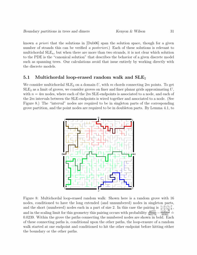
We consider multichordal SLE2 on a domain U , with m chords connecting 2m points. To getSLE2 as a limit of groves, we consider groves on finer and finer planar grids approximating U ,with n = 4m nodes, where each of the 2m SLE-endpoints is associated to a node, and each ofthe 2m intervals between the SLE-endpoints is wired together and associated to a node. (SeeFigure 8.) The “interval” nodes are required to be in singleton parts of the correspondinggrove partition, and the point nodes are required to be in doubleton parts. By Lemma 4.1, to
12
3
4
56
7
8
Figure 8: Multichordal loop-erased random walk: Shown here is a random grove with 16nodes, conditioned to have the long extended (and unnumbered) nodes in singleton parts,and the short (numbered) nodes each in a part of size 2. In this case the pairing is 1
4 | 32 | 56 | 78 ,
and in the scaling limit for this geometry this pairing occurs with probability 48777965776
− 1135√
260361
.=
0.0239. Within the grove the paths connecting the numbered nodes are shown in bold. Eachof these connecting paths is, conditional upon the other paths, the loop-erasure of a randomwalk started at one endpoint and conditioned to hit the other endpoint before hitting eitherthe boundary or the other paths.
Boundary partitions in trees and dimers Kenyon & Wilson 32
compute the SLE2 connection probabilities it is sufficient to compute the current responsesamongst the point nodes (when the interval nodes are grounded), and substitute these valuesinto the “L” polynomials associated with pairings of these 2m point nodes.
By conformal invariance, we may without loss of generality fix U to be the upper half-plane, with point nodes at x1, . . . , x2m ∈ R, and we assume that no point node is at ∞.We approximate the upper half-plane with the upper half cartesian lattice εZ × εN, andround xi to the nearest lattice point x
(ε)i ∈ εZ × εN, and let each edge have unit resistance.
The current response between distinct nodes x(ε)i and x
(ε)j is (assuming the nodes are non-
adjacent) the voltage at the vertex one lattice spacing above x(ε)j when x
(ε)i is at one volt and
the remainder of the real axis is at zero volts, which is the probability that a random walkstarted one lattice spacing above x
(ε)j ends up at x
(ε)i when it first hits the real axis, which is
Li,j = (1 + o(1))1
π
ε2
(xi − xj)2, (13)
see e.g. [Spi76, Chapter III §15], where the o(1) term goes to 0 as ε goes to 0.When we consider the ratios of these probabilities, the ε2/π factors drop out and we can
then take the limit ε → 0. We find then that Li,j is inversely proportional to the square ofthe distance between points xi and xj .
In the bichordal case, the normalized probabilities are
....Pr(12|34) =L12|34 − L13|24....Pr(14|23) =L14|23 − L13|24.
In the ε → 0 limit, the unnormalized probability (conditional on there being two chords) is
Pr(14|23) =
....Pr(14|23)
....Pr(14|23) +
....Pr(12|34)
→1
(x1−x4)21
(x2−x3)2− 1
(x1−x3)21
(x2−x4)2
1(x1−x2)2
1(x3−x4)2
+ 1(x1−x4)2
1(x2−x3)2
− 2 1(x1−x3)2
1(x2−x4)2
.
If we let s denote the cross ratio s = (x4 − x3)(x2 − x1)/[(x4 − x2)(x3 − x1)], this limitingprobability can be written as
=2s3 − s4
1 − 2s + 4s3 − 2s4,
which agrees with the known formula for bichordal SLE2, see [BBK05, § 8.2 and 8.3] [SW05][Dub06, § 4.1 and 4.2].

Boundary partitions in trees and dimers Kenyon & Wilson 33
For trichordal SLE2, the relevant polynomials are
....Pr(12|34|56) = − L15|26|34 + L12|56|34 + L14|26|35 + L15|24|36
− L14|25|36 + L13|25|46 − L12|35|46 − L13|24|56....Pr(16|23|45) = − L16|24|35 + L14|26|35 + L15|24|36 − L14|25|36
+ L16|23|45 − L13|26|45 − L15|23|46 + L13|25|46....Pr(14|23|56) =L15|24|36 − L14|25|36 − L15|23|46 + L13|25|46 + L14|23|56 − L13|24|56....Pr(25|16|34) =L16|25|34 − L15|26|34 − L16|24|35 + L14|26|35 + L15|24|36 − L14|25|36....Pr(36|12|45) =L14|26|35 − L12|46|35 − L14|25|36 − L13|26|45 + L12|36|45 + L13|25|46.
5.2 Grove Peano curves and multichordal SLE8
We can do a similar calculation for multichordal SLE8 containing m chords connecting 2mpoints. Lawler, Schramm, and Werner [LSW04] showed that on a fine grid in which part ofthe boundary is wired and part is free, the path separating a random spanning tree from itsdual spanning tree converges to chordal SLE8 connecting the two boundary points where theboundary conditions change from wired to free. If the boundary conditions alternate betweenwired and free and back m times, there will be m paths separating a random grove from its
1
4
2
3
1 2 3
4
567
8
Figure 9: The multichordal Peano curves (which converge to SLE8) associated to a grovewith four nodes (the extended black segments). In this case the grove partition is 1|2|34,which gives the Peano curve pairing 1
2 | 34 | 5
8 | 76 . In the scaling limit for this geometry these
connections occur with probability (2 −√
2)/8.= 0.0732.
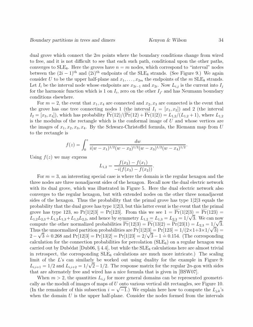
Boundary partitions in trees and dimers Kenyon & Wilson 34
dual grove which connect the 2m points where the boundary conditions change from wiredto free, and it is not difficult to see that each such path, conditional upon the other paths,converges to SLE8. Here the groves have n = m nodes, which correspond to “interval” nodesbetween the (2i − 1)th and (2i)th endpoints of the SLE8 strands. (See Figure 9.) We againconsider U to be the upper half-plane and x1, . . . , x2m the endpoints of the m SLE8 strands.Let Ii be the interval node whose endpoints are x2i−1 and x2i. Now Li,j is the current into Ij
for the harmonic function which is 1 on Ii, zero on the other Ij′ and has Neumann boundaryconditions elsewhere.
For m = 2, the event that x1, x4 are connected and x2, x3 are connected is the event thatthe grove has one tree connecting nodes 1 (the interval I1 = [x1, x2]) and 2 (the intervalI2 = [x3, x4]), which has probability
....Pr(12)/(
....Pr(12) +
....Pr(1|2)) = L1,2/(L1,2 + 1), where L1,2
is the modulus of the rectangle which is the conformal image of U and whose vertices arethe images of x1, x2, x3, x4. By the Schwarz-Christoffel formula, the Riemann map from Uto the rectangle is
f(z) =
∫ z
0
dw
i(w − x1)1/2(w − x2)1/2(w − x3)1/2(w − x4)1/2.
Using f(z) we may express
L1,2 =f(x2) − f(x1)
−i(f(x3) − f(x2)).
For m = 3, an interesting special case is where the domain is the regular hexagon and thethree nodes are three nonadjacent sides of the hexagon. Recall now the dual electric networkwith its dual grove, which was illustrated in Figure 5. Here the dual electric network alsoconverges to the regular hexagon, but with extended nodes on the other three nonadjacentsides of the hexagon. Thus the probability that the primal grove has type 1|2|3 equals theprobability that the dual grove has type 1|2|3, but this latter event is the event that the primalgrove has type 123, so Pr[1|2|3] = Pr[123]. From this we see 1 =
....Pr(1|2|3) =
....Pr(123) =
L1,2L2,3+L1,2L1,3+L1,3L2,3, and hence by symmetry L1,2 = L1,3 = L2,3 = 1/√
3. We can nowcompute the other normalized probabilities
....Pr(12|3) =
....Pr(13|2) =
....Pr(23|1) = L2,3 = 1/
√3.
Thus the unnormalized partition probabilities are Pr[1|2|3] = Pr[123] = 1/(2×1+3×1/√
3) =2−
√3
.= 0.268 and Pr[12|3] = Pr[13|2] = Pr[1|23] = 2/
√3− 1
.= 0.154. (The corresponding
calculation for the connection probabilities for percolation (SLE6) on a regular hexagon wascarried out by Dubedat [Dub06, § 4.4], but while the SLE8 calculations here are almost trivialin retrospect, the corresponding SLE6 calculations are much more intricate.) The scalinglimit of the L’s can similarly be worked out using duality for the example in Figure 9:Li,i+1 = 1/2 and Li,i+2 = 1/
√2−1/2. The response matrix for the regular 2n-gon with sides
that are alternately free and wired has a nice formula that is given in [BSW07].When m > 2, the quantities Li,j for more general domains can be represented geometri-
cally as the moduli of images of maps of U onto various vertical slit rectangles, see Figure 10.(In the remainder of this subsection i =
√−1.) We explain here how to compute the Lj,k’s
when the domain U is the upper half-plane. Consider the nodes formed from the intervals
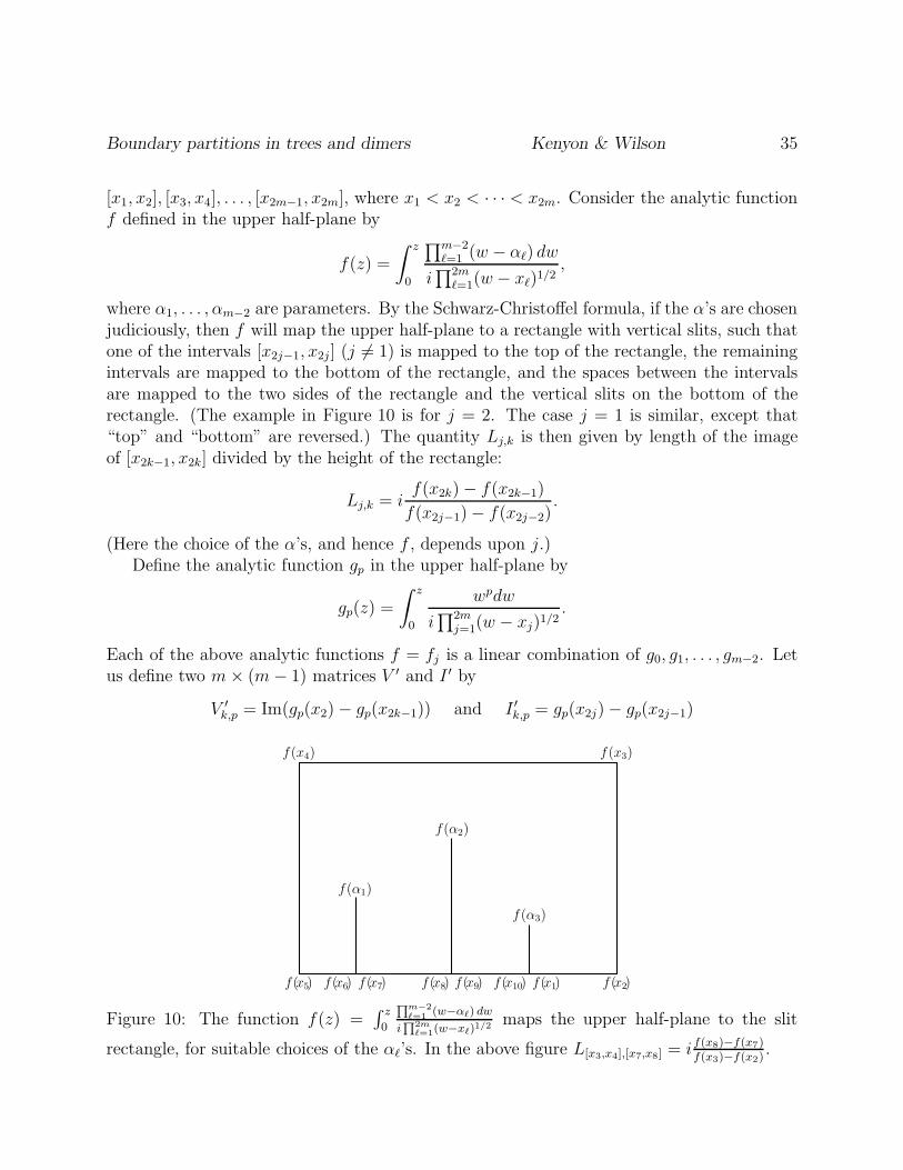
Boundary partitions in trees and dimers Kenyon & Wilson 35
[x1, x2], [x3, x4], . . . , [x2m−1, x2m], where x1 < x2 < · · · < x2m. Consider the analytic functionf defined in the upper half-plane by
f(z) =
∫ z
0
∏m−2ℓ=1 (w − αℓ) dw
i∏2m
ℓ=1(w − xℓ)1/2,
where α1, . . . , αm−2 are parameters. By the Schwarz-Christoffel formula, if the α’s are chosenjudiciously, then f will map the upper half-plane to a rectangle with vertical slits, such thatone of the intervals [x2j−1, x2j ] (j 6= 1) is mapped to the top of the rectangle, the remainingintervals are mapped to the bottom of the rectangle, and the spaces between the intervalsare mapped to the two sides of the rectangle and the vertical slits on the bottom of therectangle. (The example in Figure 10 is for j = 2. The case j = 1 is similar, except that“top” and “bottom” are reversed.) The quantity Lj,k is then given by length of the imageof [x2k−1, x2k] divided by the height of the rectangle:
Lj,k = if(x2k) − f(x2k−1)
f(x2j−1) − f(x2j−2).
(Here the choice of the α’s, and hence f , depends upon j.)Define the analytic function gp in the upper half-plane by
gp(z) =
∫ z
0
wpdw
i∏2m
j=1(w − xj)1/2.
Each of the above analytic functions f = fj is a linear combination of g0, g1, . . . , gm−2. Letus define two m × (m − 1) matrices V ′ and I ′ by
V ′k,p = Im(gp(x2) − gp(x2k−1)) and I ′
k,p = gp(x2j) − gp(x2j−1)
f(x5) f(x7) f(x9) f(x1)f(x6) f(x8) f(x10) f(x2)
f(α1)
f(α2)
f(α3)
f(x3)f(x4)
Figure 10: The function f(z) =∫ z
0
Qm−2
ℓ=1(w−αℓ) dw
iQ
2mℓ=1
(w−xℓ)1/2maps the upper half-plane to the slit
rectangle, for suitable choices of the αℓ’s. In the above figure L[x3,x4],[x7,x8] = if(x8)−f(x7)f(x3)−f(x2)
.

Boundary partitions in trees and dimers Kenyon & Wilson 36
Since for any j 6= 1, we can express fj as a linear combination of the gp’s, this same linearcombination of the columns of V ′ will be nonzero (the height of the slit rectangle) at row jand zero elsewhere, and the same linear combination of the columns of I ′ gives the lengthsof the images of the intervals in the slit rectangle. Thus V ′ has rank m − 1, and since thefirst row is all 0, we may adjoin an mth column which is all 1 to get a nonsingular matrix V ,and adjoin an mth column to I ′ which is all 0 to get a matrix I. Then for any vector ~v, wehave LV ~v = I~v, which allows us to compute L by
L = IV −1.
Thus we may compute the limiting connection probabilities completely mechanically.
5.3 Double-dimer crossings — multichordal SLE4?
There is a lot of evidence to support the hypothesis that the scaling limit of chains in thedouble-dimer model is given by SLE4, but this has not yet been rigorously proved. Theformulas given here, which are for double-dimer path scaling limits, agree with the formulasfor SLE4 (see also Section 5.4), and so provide further evidence supporting this hypothesis.
As in Section 5.1, we approximate the upper half-plane with the upper half cartesianlattice εZ×εN, and consider a set of black nodes near the points x1, x3, . . . , x2m−1 and white
nodes near the points x2, x4, . . . , x2m, letting node i be the nearest lattice point x(ε)i ∈ εZ×εN
to xi which has the appropriate color. From [Ken00, § 5.2] we have
Xi,j = (1 + o(1))2
π
ε
|xi − xj |. (14)
For the double-dimer model we can easily recover the cross-ratio formula that is knownfor bichordal SLE4 [BBK05, § 8.2 and 8.3] [SW05] [Dub06, § 4.1] as follows:
Pr(12|34) =X1,2X3,4
Pr(14|23) =X1,4X3,2
When x1 < x2 < x3 < x4, in the scaling limit ε → 0 we get
Pr(14|23) =Pr(14|23)
Pr(12|34) + Pr(14|23)→
1|x1−x4|
1|x2−x3|
1|x1−x2|
1|x4−x3| + 1
|x1−x4|1
|x2−x3|
=(x2 − x1)(x4 − x3)
(x3 − x1)(x4 − x2)
which is the formula for the cross-ratio.
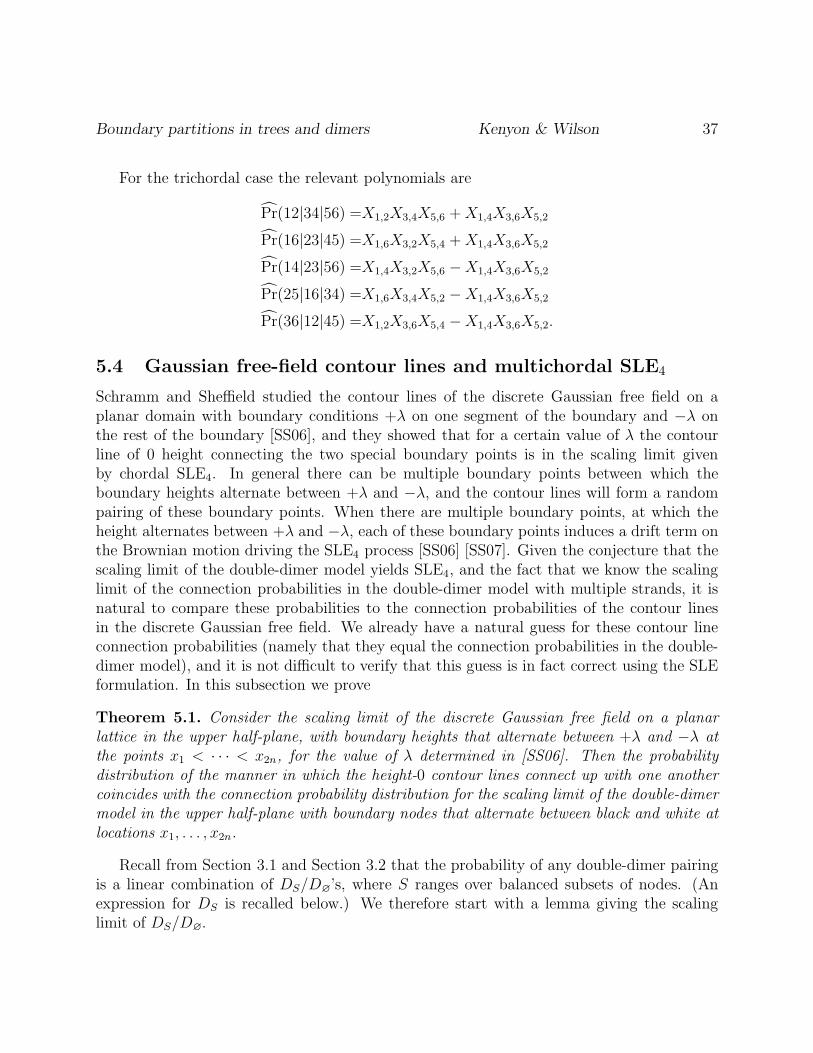
Boundary partitions in trees and dimers Kenyon & Wilson 37
For the trichordal case the relevant polynomials are
Pr(12|34|56) =X1,2X3,4X5,6 + X1,4X3,6X5,2
Pr(16|23|45) =X1,6X3,2X5,4 + X1,4X3,6X5,2
Pr(14|23|56) =X1,4X3,2X5,6 − X1,4X3,6X5,2
Pr(25|16|34) =X1,6X3,4X5,2 − X1,4X3,6X5,2
Pr(36|12|45) =X1,2X3,6X5,4 − X1,4X3,6X5,2.
5.4 Gaussian free-field contour lines and multichordal SLE4
Schramm and Sheffield studied the contour lines of the discrete Gaussian free field on aplanar domain with boundary conditions +λ on one segment of the boundary and −λ onthe rest of the boundary [SS06], and they showed that for a certain value of λ the contourline of 0 height connecting the two special boundary points is in the scaling limit givenby chordal SLE4. In general there can be multiple boundary points between which theboundary heights alternate between +λ and −λ, and the contour lines will form a randompairing of these boundary points. When there are multiple boundary points, at which theheight alternates between +λ and −λ, each of these boundary points induces a drift term onthe Brownian motion driving the SLE4 process [SS06] [SS07]. Given the conjecture that thescaling limit of the double-dimer model yields SLE4, and the fact that we know the scalinglimit of the connection probabilities in the double-dimer model with multiple strands, it isnatural to compare these probabilities to the connection probabilities of the contour linesin the discrete Gaussian free field. We already have a natural guess for these contour lineconnection probabilities (namely that they equal the connection probabilities in the double-dimer model), and it is not difficult to verify that this guess is in fact correct using the SLEformulation. In this subsection we prove
Theorem 5.1. Consider the scaling limit of the discrete Gaussian free field on a planarlattice in the upper half-plane, with boundary heights that alternate between +λ and −λ atthe points x1 < · · · < x2n, for the value of λ determined in [SS06]. Then the probabilitydistribution of the manner in which the height-0 contour lines connect up with one anothercoincides with the connection probability distribution for the scaling limit of the double-dimermodel in the upper half-plane with boundary nodes that alternate between black and white atlocations x1, . . . , x2n.
Recall from Section 3.1 and Section 3.2 that the probability of any double-dimer pairingis a linear combination of DS/D∅’s, where S ranges over balanced subsets of nodes. (Anexpression for DS is recalled below.) We therefore start with a lemma giving the scalinglimit of DS/D∅.

Boundary partitions in trees and dimers Kenyon & Wilson 38
Lemma 5.2. In the scaling limit of the double-dimer model in the upper half-plane, if thenodes are located at x1 < · · · < x2n and the node colors alternate between black and white,and if S is a balanced subset of the nodes, then
DS
D∅
=∏
i∈S,j /∈S
|xj − xi|(−1)1+i+j
.
Proof. Recall that for a set S of nodes with equal numbers of odd and even nodes, we defined
DS = det[(1i,j∈S + 1i,j /∈S) × (−1)(|i−j|−1)/2Xi,j ]i=1,3,...2n−1j=2,4,...2n
which, in the scaling limit, using Equation 14, when x1 < x2 < · · · < x2n, is given by
= det
[(1i,j∈S + 1i,j /∈S) × (−1)(|i−j|−1)/2
xj − xi
]i=1,3,...2n−1
j=2,4,...2n
= ± det
[1
xj − xi
]i odd, i ∈ S
j even, j ∈ S
det
[1
xj − xi
]i odd, i /∈ S
j even, j /∈ S
which is a product of two Cauchy determinants
= ±
∏
i<ji + j even
i, j ∈ S or i, j /∈ S
(xj − xi)
∏
i<ji + j odd
i, j ∈ S or i, j /∈ S
(xj − xi)
where the i, j ∈ S factors are from the first determinant, and the i, j /∈ S factors are fromthe second determinant. Since each multiplicand is positive and by Lemma 3.2 DS is a ratioof positive quantities, the global sign is +.
We may evaluate the ratioDS
D∅
=∏
i<j
(xj − xi)αi,j
where
αi,j =
{0, if i, j ∈ S or i, j /∈ S,
(−1)1+i+j, if i ∈ S and j /∈ S or vice versa.
We remark that products of the form∏
i<j(xj − xi)∗i,j also arise in [Dub06].
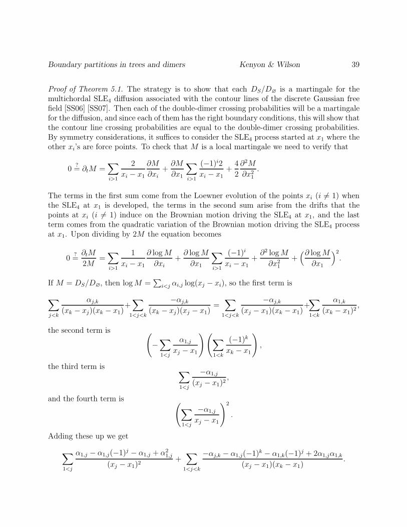
Boundary partitions in trees and dimers Kenyon & Wilson 39
Proof of Theorem 5.1. The strategy is to show that each DS/D∅ is a martingale for themultichordal SLE4 diffusion associated with the contour lines of the discrete Gaussian freefield [SS06] [SS07]. Then each of the double-dimer crossing probabilities will be a martingalefor the diffusion, and since each of them has the right boundary conditions, this will show thatthe contour line crossing probabilities are equal to the double-dimer crossing probabilities.By symmetry considerations, it suffices to consider the SLE4 process started at x1 where theother xi’s are force points. To check that M is a local martingale we need to verify that
0?= ∂tM =
∑
i>1
2
xi − x1
∂M
∂xi+
∂M
∂x1
∑
i>1
(−1)i2
xi − x1+
4
2
∂2M
∂x21
.
The terms in the first sum come from the Loewner evolution of the points xi (i 6= 1) whenthe SLE4 at x1 is developed, the terms in the second sum arise from the drifts that thepoints at xi (i 6= 1) induce on the Brownian motion driving the SLE4 at x1, and the lastterm comes from the quadratic variation of the Brownian motion driving the SLE4 processat x1. Upon dividing by 2M the equation becomes
0?=
∂tM
2M=∑
i>1
1
xi − x1
∂ log M
∂xi
+∂ log M
∂x1
∑
i>1
(−1)i
xi − x1
+∂2 log M
∂x21
+(∂ log M
∂x1
)2
.
If M = DS/D∅, then log M =∑
i<j αi,j log(xj − xi), so the first term is
∑
j<k
αj,k
(xk − xj)(xk − x1)+∑
1<j<k
−αj,k
(xk − xj)(xj − x1)=∑
1<j<k
−αj,k
(xj − x1)(xk − x1)+∑
1<k
α1,k
(xk − x1)2,
the second term is (−∑
1<j
α1,j
xj − x1
)(∑
1<k
(−1)k
xk − x1
),
the third term is ∑
1<j
−α1,j
(xj − x1)2,
and the fourth term is (∑
1<j
−α1,j
xj − x1
)2
.
Adding these up we get
∑
1<j
α1,j − α1,j(−1)j − α1,j + α21,j
(xj − x1)2+∑
1<j<k
−αj,k − α1,j(−1)k − α1,k(−1)j + 2α1,jα1,k
(xj − x1)(xk − x1).

Boundary partitions in trees and dimers Kenyon & Wilson 40
If α1,j 6= 0, then α1,j = (−1)j , so the numerators in the first sum are all 0. For the secondsum, there are a few cases to consider. If αj,k 6= 0 then αj,k = (−1)1+j+k, and either α1,j = 0or else α1,k = 0 but not both, so the numerator simplifies to 0. If αj,k = 0 then eitherα1,j = α1,k = 0 (in which case the numerator simplifies to 0), or else α1,j = (−1)j andα1,k = (−1)k, and the numerator again simplifies to 0. Thus DS/D∅ is a local martingale.Since DS/D∅ is the probability that no node in S is paired to a node in Sc (in the double-dimer model), it is bounded, and therefore it is actually a martingale.
Acknowledgement
We thank Dylan Thurston for helpful discussions.
A The response matrix
To a pair (G,N) consisting of a graph and a subset N of its vertices is associated an |N|×|N|matrix Λ, the response matrix, or Dirichlet-to-Neumann matrix. It is a real symmetricmatrix defined from the Laplacian matrix as follows. The variables Li,j used in this articleare negatives of the entries of this matrix: Li,j = −Λi,j.
A.1 Definition
Let ∆ be the Laplacian matrix of G, defined on functions on the vertices of G by ∆(f)(v) =∑w∼v cv,w(f(v)− f(w)), where the sum is over neighbors w of v and cv,w is the edge weight.
Let N be the set of nodes of G and I = V r N the inner vertices. Then RV = R
N ⊕ RI. In
this ordering, we can write
∆ =
(F GH K
)
where K is an |I| × |I| matrix.Let V ∈ R
N be a choice of potentials at the nodes. If we hold the nodes at thesepotentials, the resulting current flow in the network will have divergence zero except at thenodes, that is, (
F GH K
)(vN
vI
)=
(cN0
),
where cN ∈ RN is the vector of currents exiting the network at the nodes.
In particular we must have vI = −K−1HvN and so (F−GK−1H)vN = cN. (The matrix Kis invertible since it is the Dirichlet Laplacian on I with nonempty boundary N.) The matrixΛ = F − GK−1H satisfies
ΛvN = cN
Boundary partitions in trees and dimers Kenyon & Wilson 41
and is called the response matrix, or Dirichlet-to-Neumann matrix of the pair (G,N), and isalso known as the Schur complement ∆/K. It is a symmetric positive semidefinite matrixfrom R
N to RN with kernel consisting of the “all ones” vector [CdV98].
The following lemma is a special case of a more general determinant formula, but weneed this special case in Section 2, so we prove it here.
Lemma A.1. Pr(tree)/ Pr(uncrossing) = det Λ, where Λ is obtained from Λ by removingany row and column.
Proof. Since K is the Dirichlet Laplacian for the graph G/N in which all vertices in N
have been identified, by the matrix-tree theorem (often attributed to Kirchhoff, see [vLW92,Chapter 34]), det K is the weighted sum of spanning trees of G/N. These lift to completelydisconnected groves of G, so det K = Z(uncrossing), where Z(τ) denotes the weighted sumof groves of partition type τ , in this case 1|2| · · · |n.
Let ∆ε = ∆+εIN; recall that this is the Dirichlet Laplacian for the graph G′ obtained fromG by adjoining an external vertex connected to every vertex in N by an edge of weight ε,i.e., ∆ε is obtained from ∆(G′) by striking out the row and column corresponding to theadjoined external vertex, so that limε→0 det(∆ + εIN)/ε = nZ(tree).
Let Λε = ∆ε/K = F + εIN − GK−1H . Then
∆ε =
(Λε GK−1
0 II
)(IN 0H K
),
so det ∆ε = det Λε det K (a standard fact about Schur complements).But if Λ denotes Λ with a row and column removed, then det Λ = 1
nlimε→0(det Λε)/ε =
1n
limε→0(det ∆ε)/ε/ detK = Z(tree)/Z(uncrossing).
A.2 Relation between the Li,j’s and Ri,j’s
The Λ matrix is related to the matrix of pairwise resistances between the nodes as follows.We assume here for convenience that the electrical network is connected.
Proposition A.2. We have
Ri,j = (δi − δj)T Λ−1(δi − δj).
Note that the right hand side is well defined since δi − δj is in the image of Λ, and theinverse image of this vector is well-defined up to addition of an element of the kernel of Λ,which is perpendicular to δi − δj .
Proof. Find v ∈ RV such that Λv = −δi + δj . This represents the (unique up to an additive
constant) choice of potentials for which there is one unit of current flowing into the circuitat i and out at j. By definition, the resistance between i and j is the difference in potentialsat i and j for this current flow.

Boundary partitions in trees and dimers Kenyon & Wilson 42
The equation of Proposition A.2 can be given in a computationally simpler form asfollows. When finding v ∈ R
V such that Λv = −δi + δj , we may choose v so that vn = 0,and let v denote v with vn dropped. Let Λ be the matrix obtained from Λ by deleting thelast row and column. Then Λv = −δi + δj, where δn is interpreted as 0. By the matrix-treetheorem, Λ is invertible since det Λ is the weighted sum of spanning trees with edge weightsgiven by −Λi,j . Thus Ri,n = Λ−1
i,i , and if i, j 6= n then
Ri,j = (δi − δj)T Λ−1(δi − δj). (15)
Reciprocally to Proposition A.2 we can write Λ in terms of R as follows:
Proposition A.3. We have Λ−1i,i = Ri,n, and
Λ−1i,j =
1
2(Ri,n + Rj,n − Ri,j).
Proof. This is just the inverse of the transformation in (15).
B Complete list of grove probabilities on 4 nodes
Here we give the formulas for the planar partition probabilities when there are 4 nodes.There are 14 planar partitions on 4 nodes, but for each class of planar partitions that maybe obtained from one another by cyclically rotating and/or reversing the indices, we needonly give the formula for one representative planar partition in the class.
Pr(1234) =1,
Pr(2|143) =12R2,3 + 1
2R1,2 − 1
2R1,3,
Pr(14|23) =12R1,3 + 1
2R2,4 − 1
2R1,4 − 1
2R2,3,
Pr(1|2|34) =(+R1,2R1,3 + R1,2R2,3 + R1,2R1,4 + R1,2R2,4 − 2R1,2R3,4 − R21,2
+ R1,3R2,4 + R1,4R2,3 − R1,3R1,4 − R2,3R2,4)/4,
Pr(1|3|24) =(+R1,3R1,2 + R1,3R2,3 + R1,3R1,4 + R1,3R3,4 − 2R1,3R2,4 − R21,3
+ R1,2R3,4 + R1,4R2,3 − R1,2R1,4 − R2,3R3,4)/4,
Pr(1|2|3|4) =(+R1,2R2,3R3,4 + R1,2R2,4R4,3 + R1,3R3,2R2,4 + R1,3R3,4R4,2
+ R1,4R4,2R2,3 + R1,4R4,3R3,2 + R2,1R1,3R3,4 + R2,1R1,4R4,3
+ R2,3R3,1R1,4 + R2,4R4,1R1,3 + R3,1R1,2R2,4 + R3,2R2,1R1,4
− R1,2R2,3R3,1 − R1,2R2,4R4,1 − R1,3R3,4R4,1 − R2,3R3,4R4,2
− R1,2R23,4 − R2
1,2R3,4 − R1,3R22,4 − R2
1,3R2,4 − R1,4R22,3 − R2
1,4R2,3)/4.
Boundary partitions in trees and dimers Kenyon & Wilson 43
Equivalently,
....Pr(1234) =L1234 =L1,2L1,3L1,4 + L1,2L2,3L2,4 + L1,3L2,3L3,4 + L1,4L2,4L3,4+
L1,2L2,3L3,4 + L1,3L2,3L2,4 + L1,2L2,4L3,4 + L1,4L2,3L2,4+
L1,2L1,3L2,4 + L1,2L1,4L2,3 + L1,3L2,4L3,4 + L1,4L2,3L3,4+
L1,3L1,4L2,3 + L1,2L1,3L3,4 + L1,3L1,4L2,4 + L1,2L1,4L3,4,....Pr(2|143) =L2|143 + L13|24 =L1,3L1,4 + L1,4L3,4 + L1,3L3,4 + L1,3L2,4,....Pr(14|23) =L14|23 − L13|24 =L1,4L2,3 − L1,3L2,4,....Pr(1|2|34) =L1|2|34 =L3,4,....Pr(1|3|24) =L1|3|24 =L2,4,....Pr(1|2|3|4) =L1|2|3|4 =1.
References
[ASA02] Louis-Pierre Arguin and Yvan Saint-Aubin. Non-unitary observables inthe 2d critical Ising model. Physics Letters B, 541(3-4):384–389, 2002,arXiv:hep-th/0109138. MR1928682 (2003h:82016)
[BBK05] Michel Bauer, Denis Bernard, and Kalle Kytola. Multiple Schramm-Loewnerevolutions and statistical mechanics martingales. J. Stat. Phys., 120(5-6):1125–1163, 2005, arXiv:math-ph/0503024. MR2187598 (2007d:82032)
[BSW07] Nathaniel D. Blair-Stahn and David B. Wilson. The electrical response matrixof a regular 2n-gon, 2007, arXiv:math.CA/0703826. Proc. Amer. Math. Soc., toappear.
[Car92] John L. Cardy. Critical percolation in finite geometries. J. Phys. A, 25(4):L201–L206, 1992, arXiv:math-ph/9910002. MR1151081 (92m:82048)
[Car07] John Cardy. ADE and SLE. J. Phys. A, 40(7):1427–1438, 2007,arXiv:math-ph/0610030. MR2303259 (2008k:82023)
[CdV98] Yves Colin de Verdiere. Spectres de Graphes, volume 4 of Cours Specialises[Specialized Courses]. Societe Mathematique de France, Paris, 1998.MR1652692 (99k:05108)
[CIM98] E. B. Curtis, D. Ingerman, and J. A. Morrow. Circular planar graphsand resistor networks. Linear Algebra Appl., 283(1-3):115–150, 1998.MR1657214 (99k:05096)
Boundary partitions in trees and dimers Kenyon & Wilson 44
[Ciu97] Mihai Ciucu. Enumeration of perfect matchings in graphs with reflective sym-metry. J. Combin. Theory Ser. A, 77(1):67–97, 1997. MR1426739 (98a:05112)
[CN07] Federico Camia and Charles M. Newman. Critical percolation exploration pathand SLE6: a proof of convergence. Probab. Theory Related Fields, 139(3-4):473–519, 2007, arXiv:math/0604487. MR2322705 (2008k:82040)
[CS04] Gabriel D. Carroll and David Speyer. The cube recurrence. Electron. J.Combin., 11(1):Research Paper 73, 31 pp., 2004, arXiv:math.CO/0403417.MR2097339 (2005f:05007)
[DFGG97] P. Di Francesco, O. Golinelli, and E. Guitter. Meanders and the Temperley-Lieb algebra. Comm. Math. Phys., 186(1):1–59, 1997, arXiv:hep-th/9602025.MR1462755 (99f:82028)
[DS84] Peter G. Doyle and J. Laurie Snell. Random Walks and Electric Networks, vol-ume 22 of Carus Mathematical Monographs. Mathematical Association of Amer-ica, Washington, DC, 1984, arXiv:math.PR/0001057. MR920811 (89a:94023)
[DS87] B. Duplantier and H. Saleur. Exact critical properties of two-dimensionaldense self-avoiding walks. Nuclear Phys. B, 290(3):291–326, 1987.MR919521 (89g:82049)
[Dub06] Julien Dubedat. Euler integrals for commuting SLEs. J. Stat. Phys., 123(6):1183–1218, 2006, arXiv:math.PR/0507276. MR2253875 (2007g:82027)
[Dup87] Bertrand Duplantier. Critical exponents of Manhattan Hamiltonian walks intwo dimensions, from Potts and O(n) models. J. Statist. Phys., 49(3-4):411–431,1987. MR926190 (89b:82025)
[Dup89] Bertrand Duplantier. Statistical mechanics of polymer networks of any topology.J. Statist. Phys., 54(3-4):581–680, 1989. MR988554 (90e:82061)
[Dup92] Bertrand Duplantier. Loop-erased self-avoiding walks in two dimensions: exactcritical exponents and winding numbers. Physica A, 191:516–522, 1992.
[Dup06] Bertrand Duplantier. Conformal random geometry. In A. Bovier, F. Dunlop,A. van Enter, F. den Hollander, and J. Dalibard, editors, Mathematical StatisticalPhysics, Lecture Notes of the Les Houches Summer School Session LXXXIII,2005, pages 101–217. Elsevier, 2006, arXiv:math-ph/0608053.
[Fom01] Sergey Fomin. Loop-erased walks and total positivity. Trans. Amer.Math. Soc., 353(9):3563–3583 (electronic), 2001, arXiv:math.CO/0004083.MR1837248 (2002f:15030)
Boundary partitions in trees and dimers Kenyon & Wilson 45
[Jon83] V. F. R. Jones. Index for subfactors. Invent. Math., 72(1):1–25, 1983.MR696688 (84d:46097)
[Kas67] P. W. Kasteleyn. Graph theory and crystal physics. In Graph The-ory and Theoretical Physics, pages 43–110. Academic Press, London, 1967.MR0253689 (40 #6903)
[Ken97] Richard Kenyon. Local statistics of lattice dimers. Ann. Inst. H. Poincare Probab.Statist., 33(5):591–618, 1997, arXiv:math.CO/0105054. MR1473567 (99b:82039)
[Ken00] Richard Kenyon. Conformal invariance of domino tiling. Ann. Probab., 28(2):759–795, 2000, arXiv:math-ph/9910002. MR1782431 (2002e:52022)
[Kir90] Gustav Kirchhoff. Beweis der Existenz des Potentials das an der Grenze desbetrachteten Raumes gegebene Werthe hat fur den Fall dass diese Grenze eineuberall convexe Flache ist. Acta Math., 14(1):179–183, 1890. MR1554794
[KL07] Michael J. Kozdron and Gregory F. Lawler. The configurational measure onmutually avoiding SLE paths. In Universality and Renormalization, volume 50of Fields Inst. Commun., pages 199–224. Amer. Math. Soc., Providence, RI, 2007,arXiv:math.PR/0605159. MR2310306 (2008m:60079)
[KS91] Ki Hyoung Ko and Lawrence Smolinsky. A combinatorial matrix in 3-manifoldtheory. Pacific J. Math., 149(2):319–336, 1991. MR1105701 (92d:57008)
[Kuo04] Eric H. Kuo. Applications of graphical condensation for enumeratingmatchings and tilings. Theoretical Computer Science, 319(1-3):29–57, 2004,arXiv:math.CO/0304090.
[KW08] Richard W. Kenyon and David B. Wilson. Combinatorics of tripartite boundaryconnections for trees and dimers, 2008, arXiv:0811.1766.
[LSW04] Gregory F. Lawler, Oded Schramm, and Wendelin Werner. Conformal invarianceof planar loop-erased random walks and uniform spanning trees. Ann. Probab.,32(1B):939–995, 2004, arXiv:math.PR/0112234. MR2044671 (2005f:82043)
[OB88] Kaoru Ohno and Kurt Binder. Scaling theory of star polymers and general poly-mer networks in bulk and semi-infinite good solvents. J. Physique, 49(8):1329–1351, 1988. MR966320 (89j:82053)
[Pem95] Robin Pemantle. Uniform random spanning trees. In J. Laurie Snell, editor,Topics in Contemporary Probability and its Applications, Probab. StochasticsSer., pages 1–54. CRC, Boca Raton, FL, 1995. MR1410532 (97i:60013)
Boundary partitions in trees and dimers Kenyon & Wilson 46
[PS05] T. Kyle Petersen and David Speyer. An arctic circle theorem for Groves.J. Combin. Theory Ser. A, 111(1):137–164, 2005, arXiv:math.CO/0407171.MR2144860 (2006m:05055)
[Sal86] H. Saleur. New exact exponents for two-dimensional self-avoiding walks. J. Phys.A, 19:L807–L810, 1986.
[Sch00] Oded Schramm. Scaling limits of loop-erased random walks and uniformspanning trees. Israel J. Math., 118:221–288, 2000, arXiv:math/9904022.MR1776084 (2001m:60227)
[Sch07] Oded Schramm. Conformally invariant scaling limits (an overview anda collection of problems). In International Congress of Mathematicians.Vol. I, pages 513–543. Eur. Math. Soc., Zurich, 2007, arXiv:math/0602151.MR2334202 (2008j:60237)
[Smi01] Stanislav Smirnov. Critical percolation in the plane: conformal invariance,Cardy’s formula, scaling limits. C. R. Acad. Sci. Paris Ser. I Math., 333(3):239–244, 2001. MR1851632 (2002f:60193)
[Smi07] Stanislav Smirnov. Conformal invariance in random cluster models. I. Holomor-phic fermions in the Ising model, 2007, arXiv:0708.0039.
[Spi76] Frank Spitzer. Principles of Random Walk. Springer-Verlag, New York, secondedition, 1976. Graduate Texts in Mathematics, Vol. 34. MR0388547 (52 #9383)
[SS06] Oded Schramm and Scott Sheffield. Contour lines of the two-dimensional discreteGaussian free field, 2006, arXiv:math.PR/0605337.
[SS07] Oded Schramm and Scott Sheffield, 2007. In preparation.
[Sta86] Richard P. Stanley. Enumerative Combinatorics, Volume 1. Wadsworth &Brooks/Cole Advanced Books & Software, 1986. MR847717 (87j:05003)
[Sta99] Richard P. Stanley. Enumerative Combinatorics, Volume 2. Cambridge Studiesin Advanced Mathematics #62. Cambridge University Press, Cambridge, 1999.With an appendix by Sergey Fomin. MR1676282 (2000k:05026)
[SW05] Oded Schramm and David B. Wilson. SLE, quadrangles, and curvilinear trian-gles, 2005.
[vLW92] J. H. van Lint and R. M. Wilson. A Course in Combinatorics. CambridgeUniversity Press, Cambridge, 1992. MR1207813 (94g:05003)


![Prototype centrifugal natural gas cleaner CONFIDENTIAL · Nomenclature A area [m2] CD drag force coefficient [-] CM torque coefficient [-] D diameter [m] d diameter [m] dc channel](https://img.pdfslide.net/doc/110x75/5ecbd0d31495fb70d12dbcc0/prototype-centrifugal-natural-gas-cleaner-nomenclature-a-area-m2-cd-drag-force.jpg)