Embed Size (px)
Citation preview

Boundary-value Problems in Electrostatics I
Karl Friedrich Gauss
(1777 - 1855)
December 23, 2000
Contents
1 Method of Images 1
1.1 Point Charge Above a Conducting Plane . . . . . . . . . 2
1.2 Point Charge Between Multiple Conducting Planes . . . 4
1.3 Point Charge in a Spherical Cavity . . . . . . . . . . . . 5
1.4 Conducting Sphere in a Uniform Applied Field . . . . . . 13
2 Green’s Function Method for the Sphere 16
3 Orthogonal Functions and Expansions; Separation of
Variables 19
3.1 Fourier Series . . . . . . . . . . . . . . . . . . . . . . . . 22
3.2 Separation of Variables . . . . . . . . . . . . . . . . . . . 24
3.3 Rectangular Coordinates . . . . . . . . . . . . . . . . . . 25
3.4 Fields and Potentials on Edges . . . . . . . . . . . . . . . 29
1

4 Examples 34
4.1 Two-dimensional box with Neumann boundaries . . . . . 34
4.2 Numerical Solution of Laplace’s Equation . . . . . . . . . 37
4.3 Derivation of Eq. 35: A Mathematica Session . . . . . . 40
In this chapter we shall solve a variety of boundary value problems
using techniques which can be described as commonplace.
1 Method of Images
This method is useful given sufficiently simple geometries. It is closely
related to the Green’s function method and can be used to find Green’s
functions for these same simple geometries. We shall consider here only
conducting (equipotential) bounding surfaces which means the bound-
ary conditions take the form of Φ(x) = constant on each electrically
isolated conducting surface. The idea behind this method is that the
solution for the potential in a finite domain V with specified charge
density and potentials on its surface S can be the same within V as the
solution for the potential given the same charge density inside of V but
a quite different charge density elsewhere. Thus we consider two dis-
tinct electrostatics problems. The first is the “real” problem in which
we are given a charge density ρ(x) in V and some boundary conditions
on the surface S. The second is a “fictitious problem” in which the
charge density inside of V is the same as for the real problem and in
2

which there is some undetermined charge distribution elsewhere; this is
to be chosen such that the solution to the second problem satisfies the
boundary conditions specified in the first problem. Then the solution
to the second problem is also the solution to the first problem inside of
V (but not outside of V). If one has found the initially undetermined
exterior charge in the second problem, called image charge, then the
potential is found simply from Coulomb’s Law,
Φ(x) =∫d3x′
ρ2(x′)
|x− x′| ; (1)
ρ2 is the total charge density of the second problem.
1.1 Point Charge Above a Conducting Plane
This may sound confusing, but it is made quite clear by a simple ex-
ample. Suppose that we have a point charge q located at a point
x0 = (0, 0, a) in Cartesian coordinates. Further, a grounded conductor
occupies the half-space z < 0, which means that we have the Dirichlet
boundary condition at z = 0 that Φ(x, y, 0) = 0; also, Φ(x) → 0 as
r → ∞. The first thing that we must do is determine some image
charge located in the half-space z < 0 such that the potential of the
image charge plus the real charge (at x0) produces zero potential on the
z = 0 plane. With just a little thought one realizes that a single image
charge −q located at the point x′0 = (0, 0,−a) is what is required.
3

xx0q
-qimage charge
x
y
z
planez=0
=(0,0,a)
(0,0,-a)
All points on the z = 0 plane are equidistant from the real charge and
its image, and so the two charges produce cancelling potentials at each
of these points. The solution to the problem is therefore
Φ(x) = q
1
|x− x0|− 1
|x− x′0|
. (2)
This function satisfies the correct Poisson equation in the domain z > 0
and also satisfies the correct boundary conditions at z = 0; therefore it
is the (unique) solution. It is important to realize, however, that it is
not the correct solution in the space z < 0; here, the real potential is
zero because this domain in inside of the grounded conductor.
In the real system, there is some surface charge density σ(x, y) on
the conductor; to determine what this is, we have only to evaluate the
normal component of the electric field at the surface of the conductor,
En(x, y, 0) = − ∂Φ(x)
∂z
∣∣∣∣∣∣z=0
= − 2qa
(ρ2 + a2)3/2, (3)
4
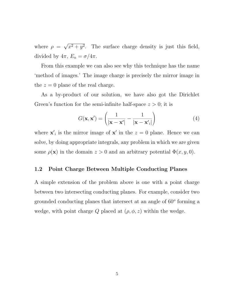
where ρ =√x2 + y2. The surface charge density is just this field,
divided by 4π, En = σ/4π.
From this example we can also see why this technique has the name
‘method of images.’ The image charge is precisely the mirror image in
the z = 0 plane of the real charge.
As a by-product of our solution, we have also got the Dirichlet
Green’s function for the semi-infinite half-space z > 0; it is
G(x,x′) =
1
|x− x′| −1
|x− x′i|
(4)
where x′i is the mirror image of x′ in the z = 0 plane. Hence we can
solve, by doing appropriate integrals, any problem in which we are given
some ρ(x) in the domain z > 0 and an arbitrary potential Φ(x, y, 0).
1.2 Point Charge Between Multiple Conducting Planes
A simple extension of the problem above is one with a point charge
between two intersecting conducting planes. For example, consider two
grounded conducting planes that intersect at an angle of 60o forming a
wedge, with point charge Q placed at (ρ, φ, z) within the wedge.
5

60o
( z)ρ,φ,Q
Q
Q
-Q
-Q
-Q
imagecharge
To solve this problem, we again use image charges to satisfy the
boundary conditions. There are five image charges, as indicated in the
figure above. They all share the same value of ρ and z as the real
charge, and their azimuthal angles are given in the table below.
charge angle
−Q 2π3 − φ
+Q 2π3 + φ
−Q −2π3 − φ
+Q −2π3 + φ
−Q −φ
1.3 Point Charge in a Spherical Cavity
It is also sometimes possible to use the image method when the bound-
ary S involves curved surfaces. However, just as curved mirrors pro-
duced distorted images, so do curved surfaces make the image of a point
6

charge more complicated1. Let’s do the simplest problem of this kind.
Suppose that we have a spherical cavity of radius a inside of a conduc-
tor; within this cavity is a point charge q located a distance r0 from the
center of the sphere which is also chosen as the origin of coordinates.
Thus the charge is at point x0 = r0n0 where n0 is a unit vector pointing
in the direction from the origin to the charge.
We need to find the image(s) of the charge in the spherical surface
which encloses it. The simplest possible set of images would be a single
charge q′; if there is such a solution, symmetry considerations tell us
that the image must be located on the line passing through the origin
and going in the direction of n0. Let us therefore put an image charge
q′ at point x′0 = r′0n0.
ax0
x0’
q
q’
V
conductor
1Consider the example of the right-hand side-view mirror of a car. Here the mirror is concave,
and images appear to be much farther away than they actually are
7

The potential produced by this charge and the real one at x0 is
Φ(x) =q
|x− x0|+
q′
|x− x′0|. (5)
Now we must choose, if possible, q′ and r′0 such that Φ(x) = 0 for x
on the cavity’s spherical surface, x = an where the direction of n is
arbitrary. The potential at such a point may be written as
Φ(an) =q/a
|n− (r0/a)n0|+
q′/r′0|n0 − (a/r′0)n|
. (6)
The from the figure below, it is clear that denominators are equal if
r0/a = a/r′0, and the numerators are equal and opposite if q/a =
−q′/r′0. (The “other” solution, r′0 = r0 and q′ = −q is no solution
at all since then the image charge would be within the volume V and
cancel the real charge. We must have r′0 > 1)
n
n
n0
n0
d2
d1
d1d2 if=0(a/r’) (r /a)0=
n0(r /a)0- 0(a/r’)n-
Hence, we make Φ zero on S by choosing
r′0 = a2/ro and q′ = −q(a/r0). (7)
8

Thus we have the solution for a point charge in a spherical cavity with
an equipotential surface:
Φ(x) = q
1
|x− x0|− a/r0
|x− (a2/r20)x0|
; (8)
we have also found the Dirichlet Green’s function for the interior of a
sphere of radius a:
G(x,x′) =1
|x− x′| −a/r
|x′ − (a2/r2)x| . (9)
The solution of the “inverse” problem which is a point charge outside
of a conducting sphere is the same, with the roles of the real charge
and the image charge reversed. The preceding equations for Φ(x) and
G(x,x′) are valid except that r, r0, and r′ are all larger than a.
Let’s look at a few more features of the solution for the charge inside
of the spherical cavity. First, what is σ, the charge density on the sur-
face of the cavity. From Gauss’s Law, we know that the charge density
is the normal component of the electric field out of the conductor at its
surface divided by 4π. This is the negative of the radial component in
spherical polar coordinates, so
σ = −Er
4π=
1
4π
∂Φ
∂r. (10)
If we define the z-direction to be the direction of n0, then the potential
at an arbitrary point within the sphere is
Φ(x) = q
1
(r2 + r20 − 2rr0 cos θ)1/2
− (a/r0)
(r2 + (a4/r20)− 2r(a2/r0) cos θ)1/2
(11)
9

where θ is the usual polar angle between the z-axis, or direction of x0,
and the direction of x, the field point. The radial component of the
electric field at r = a is
Er = − ∂Φ(x)
∂r
∣∣∣∣∣∣r=a
= −q−1
2
2a− 2r cos θ
(a2 + r20 − 2ar0 cos θ)3/2
+a
r0
1
2
2a− 2(a2/r0) cos θ
(a2 + (a4/r20)− 2(a3/r0) cos θ)3/2
= q
a− r0 cos θ
(a2 + r20 − 2ar0 cos θ)3/2
− r20
a2
a− (a2/r0) cos θ
(a2 + r20 − 2ar0 cos θ)3/2
=q
a2
1− r2
0/a2
(1 + (r20/a
2)− 2(r0/a) cos θ)3/2
(12)
If we introduce ε = r0/a, then the surface charge density may be written
concisely as
σ = − q
4πa2
1− ε2(1 + ε2 − 2ε cos θ)3/2
. (13)
The total charge on the surface may be found by integrating
over σ. But it may be obtained more easily by invoking Gauss’s Law; if
we integrate the normal component of E(x) over a closed surface which
lies entirely in conducting material and which also encloses the cavity,
we know that we will get zero, because the field in the conductor is
zero.
10

ax0
q
V
conductorGaussian surface
E=0
0 =∫
Sd2xE · n = 4πQ = 4π
(q +
∫
Sd2x σ
)
charge within this surface. What is inside is the charge q in the cavity
and the surface charge on the conductor. The implication is that the
total surface charge is equal to −q. It is perhaps useful to actually do
the integral over the surface as a check that we have gotten the charge
density there right:
Qi =∫
Sd2x σ(x)
= −q2
(1− ε2)∫ 1
−1
du
(1 + ε2 − 2εu)3/2
= −q2
1− ε22ε
2
(1 + ε2 − 2ε)1/2− 2
(1 + ε2 + 2ε)1/2
= −q2
1− ε2ε
(1
1− ε −1
1 + ε
)= −q. (14)
Notice that |σ| is largest in the direction of n0 and is
|σmax| = −q
4πa2
1 + ε
(1− ε)2. (15)
11

In the opposite direction, the magnitude of the charge density is at its
minimum which is
|σmin| = −q
4πa2
1− ε(1 + ε)2
. (16)
The total force on the charge may also be computed. This is
the negative of the total force on the conductor. Now, we know that
the force per unit area on the surface of the conductor is 2πσ2 and is
directed normal to the conductor’s surface into the cavity. Because of
the rotational invariance of the system around the direction of n0, only
the component of the force along this direction need be computed; the
other components will average to zero when integrated over the surface.
q
V
conductor
O
pThis component ofp adds.
This componentcancels.p= F/area = 2π σ2
Hence we find
|Fn| = 2πa2∫ 2π
0dφ
∫ π0
sin θdθσ2(θ) cos θ
=4π2a2q2
16π2a4(1− ε2)2
∫ 1
−1
udu
(1 + ε2 − 2εu)3=
1
4
q2
a2(1− ε2)2
∫ 1
−1
udu
(1 + ε2 − 2εu)3
=1
4
q2
a2(1− ε2)2 1
4ε2
− 1
1 + ε2 − 2εu+
1 + ε2
2(1 + ε2 − 2εu)2
1
−1
12

=1
4
q2
a2
(1− ε2)2
4ε2
−1
(1− ε)2+
1
(1 + ε)2+
1 + ε2
2(1− ε)4− 1 + ε2
2(1 + ε)4
=q2
4a2
(1− ε2)2
4ε2
−4ε
(1− ε2)2+
(1 + ε2)(8ε+ 8ε3)
2(1− ε2)4
=q2
4a2
−4ε(1− ε2)2 + 4ε(1 + ε2)2
4ε2(1− ε2)2=q2
a2
ε
(1− ε2)2.(17)
The direction of this force is such that the charge is attracted toward
the point on the cavity wall that is closest to it.
We may also ask what is the “force” between the charge and its
image. The distance between them is r′0−r0 = aε(1/ε2−1) = a(1−ε2)/ε,
and the product of the charges is qq′ = −q2/ε, so
|F| = q2
a2
ε
(1− ε2)2(18)
which is the same as the real force between the charge and the surface.
One is led to ask whether the real force on the charge is always the
same as that between the charge and its images. The answer is yes.
The electric field produced by the real surface charge at the position
of the real charge is the same as that produced by the image charge
at the real charge, and so the same force will arise in both systems. It
is generally much easier to calculate the force between the real charge
and its images than the force between the real charge and the surface
charges.
13

1.4 Conducting Sphere in a Uniform Applied Field
Consider next the example of a grounded conducting sphere, which
means that Φ(x) = 0 on the sphere, placed in a region of space where
there was initially a uniform electric field E0 = E0z produced by some
far away fixed charges. Here, z is a unit vector pointing in the z-
direction. We approach this problem by replacing it with another one
which will become equivalent to the first one in some limit. Let the
sphere be centered at the origin and let there be not a uniform applied
field but rather a charge Q placed at the point (0, 0,−d) and another
charge −Q placed at the point (0, 0, d) in Cartesian coordinates.
x
y
z
q
-q
-Q
Q
a b
db=a /d2
The resulting potential configuration is easily solved by the image
method; there are images of the charges±Q in the sphere at (0, 0,−a2/d)
and at (0, 0, a2/d); they have size −Qa/d and Qa/d, respectively. The
potential produced by these four charges is zero on the surface of the
14

sphere. Thus we have solved the problem of a grounded sphere in
the presence of two symmetrically located equal and opposite charges.
We could equally well think of the sphere as isolated (not electrically
connected to anything) and neutral, because the total image charge is
zero.
Now we want to think about what happens if we let Q become
increasingly large and at the same time move the real charges farther
and farther away from the sphere in such a way that the field they
produce at the origin is constant. This field is E(x) = (2Q/d2)z, so
if Q is increased at a rate proportional to d2, the field at the origin
is unaffected. As d becomes very large in comparison with the radius
a of the sphere, not only will the applied field at the origin have this
value, but it will have very nearly this value everywhere in the vicinity
of the sphere. The difference becomes negligible in the limit d/a→∞.
Hence we recover the configuration presented in the original problem
of a sphere placed in a uniform applied field. If we pick E0 = 2Q/d2,
or, more appropriately, Q = E0d2/2, we have the solution in the limit
of d→∞:
Φ(x) = limd→∞
E0d
2/2
(d2 + r2 + 2rd cos θ)1/2− E0d
2a/2d
(a4/d2 + r2 + 2r(a2/d) cos θ)1/2
+ limd→∞
− E0d
2/2
(d2 + r2 − 2rd cos θ)1/2+
E0d2a/2d
(a4/d2 + r2 − 2r(a2/d) cos θ)1/2
= limd→∞
± E0d/2
(1± 2(r/d) cos θ + r2/d2)1/2∓ E0da/2r
(1± (a2/rd) cos θ + a4/d2r2)1/2
15

= −E0r cos θ +E0a
3
r2cos θ.(19)
The first term, −E0r cos θ, is the potential of the applied constant field,
E0. The second is the potential produced by the induced surface charge
density on the sphere. This has the characteristic form of an electric
dipole field, of which we shall hear more presently. The dipole moment
p associated with any charge distribution is defined by the equation
p =∫d3xxρ(x); (20)
in the present case the dipole moment of the sphere may be found
either from the surface charge distribution or from the image charge
distribution. Taking the latter tack, we find
p =∫d3xx
E0da
2
[−δ(z + a2/d)δ(y)δ(x) + δ(z − a2/d)δ(y)δ(x)
]
=E0da
2
[(a2/d)z + (a2/d)z
]= E0a
3z. (21)
Comparison with the expression for the potential shows that the dipolar
part of the potential may be written as
Φ(x) = p · x/r3 (22)
The charge density on the surface of the sphere may be found in the
usual way:
4πσ = Er = − ∂Φ
∂r
∣∣∣∣∣r=a
= E0 cos θ +2E0
a3a3 cos θ = 3E0 cos θ. (23)
16

Hence,
σ(θ) =3
4πE0 cos θ. (24)
2 Green’s Function Method for the Sphere
Next, let us do an example of the use of the Green’s function method by
considering a Dirichlet potential problem inside of a sphere. The task
is to calculate the potential distribution inside of an empty (ρ(x) = 0,
x ∈ V ) spherical cavity of radius a, given some specified potential
distribution V (θ, φ) on the surface of the sphere. We can immediately
invoke the Green’s function expression
Φ(x) = − 1
4π
∫
Sd2x′Φ(x′)
∂G(x,x′)
∂n′, (25)
and we already know that,
G(x,x′) =1
|x− x′| −a/r′
|x− (a2/r′2)x′| (26)
since G(x,x′) is the potential at x due to a unit point charge at x′
(x ,x′ ∈ V ), and we have just solved this problem. If we let γ be the
angle between x and x′,
G(x,x′) =1
(r2 + r′2 − 2rr′ cos γ)1/2− a/r′
(r2 + (a4/r′2)− 2r(a2/r′) cos γ)1/2.
(27)
Then
∂G(x,x′)
∂n′
∣∣∣∣∣∣S
=∂G(x,x′)
∂r′
∣∣∣∣∣∣r′=a
17

= −1
2
2a− 2r cos γ
(r2 + a2 − 2ra cos γ)3/2− a 2ar2 − 2ra2 cos γ
(r2a2 + a4 − 2ra3 cos γ)3/2
= − a(1− r2/a2)
(r2 + a2 − 2ra cos γ)3/2= − 1
a2
(1− ε2)(1 + ε2 − 2ε cos γ)3/2
(28)
where ε = r/a. For simplicity, let us suppose that ρ(x) = 0 inside of
the sphere. Then
Φ(x) =1
4π
∫ 2π
0dφ′
∫ π0
sin θ′dθ′V (θ′, φ′)(1− ε2)(1 + ε2 − 2ε cos γ)3/2
. (29)
In terms of θ, φ and θ′ and φ′,
cos γ = cos θ cos θ′ + sin θ sin θ′ cos(φ− φ′). (30)
This integral can rarely be done in closed form in terms of simple func-
tions; however, it is generally a simple matter to carry out the integrals
numerically. As an example, consider
VΦ =
-VΦ =
V (θ, φ) =
V, 0 ≤ θ ≤ π/2
−V, π/2 ≤ θ ≤ π.(31)
Then the answer will not depend on φ, so we may arbitrarily set φ
equal to zero and proceed. Using ε ≡ r/a, we have
Φ(ε, θ) =V
4π(1−ε2)
∫ 2π
0dφ′
∫ π/2
0
sin θ′dθ′
(1 + ε2 − 2ε cos γ)3/2−∫ ππ/2
sin θ′dθ′
(1 + ε2 − 2ε cos γ)3/2
(32)
18

The integral is still difficult in the general case. For θ = 0, it is easier:
Φ(ε, 0) =V
4π(1− ε2)2π
∫ 1
0
du
(1 + ε2 − 2εu)3/2−∫ 0
−1
du
(1 + ε2 − 2εu)3/2
(33)
These integrals are easily completed with the result that
Φ(ε, 0) =V
ε
1− 1− ε2√
1 + ε2
. (34)
An alternative approach, valid for r/a << 1, is to expand the integrand
in powers of ε and then to complete the integration term by term. This
is straightforward with a symbolic manipulator but tedious by hand.
Either way, a solution in powers of ε is generated.
Φ(ε, θ) =3V
2
[ε cos θ − 7
12ε3(
5
2cos3 θ − 3
2cos θ
)+O(ε5)
]. (35)
The alert student will recognize that the functions of cos θ that are
being generated are Legendre polynomials;
P1(cos θ) = cos θ,
P3(cos θ) =5
2cos3 θ − 3
2cos θ, (36)
etc. Note that only terms which are odd in cos θ enter into the sum,
due to the symmetry of the boundary conditions.
19

3 Orthogonal Functions and Expansions; Separa-
tion of Variables
We turn now to a quite different, much more systematic approach to
the solution Laplace’s equation
∇2Φ(x) = 0 (37)
as a boundary value problem. It is implemented by expanding the
solution in some domain V using complete sets of orthogonal functions
Φ(η, ξ, ν) =∑
nlm
An(η)Bl(ξ)Cm(ν) (38)
and determining the coefficients in the expansion by requiring that
the solution take on the proper values on the boundaries. For simple
geometries for which Laplace’s equation separates (spheres, cylinders,
rectangular parallelepipeds) this method can always be utilized2. Be-
fore launching into a description of how one proceeds in specific cases
(or geometries), let us take a few minutes to review the terminology of
orthogonal function expansions and some basic facts.
Suppose that we have a set of functions Un(η), n = 1, 2,... which are
orthogonal on the interval a ≤ η ≤ b, by which we mean that
∫ badηU ∗n(η)Um(η) = 0, if m 6= n; (39)
2It can also be very tedious.
20

the superscript * denotes complex conjugation. Further, the functions
Un(η) are normalized on the interval,
∫ badηU ∗n(η)Un(η) =
∫ badη|Un(η)|2 = 1. (40)
Combining these equations we have
∫ badηU ∗n(η)Um(η) =
0, n 6= m
1, n = m
= δnm. (41)
The functions Un(η) are said to be orthonormal; δnm is called a Kro-
necker delta function.
Next, we attempt to expand, on the interval a ≤ η ≤ b, an arbitrary
function f(η) as a linear combination of the functions Un(η), which are
referred to as basis functions. Keeping just N terms in the expansion,
one has
f(η) ≈N∑
n=1
anUn(η). (42)
We need a criterion for choosing the coefficients in the expansion; a
standard criterion is to minimize the mean square error E which may
be defined as follows:
E =∫ badη|f(η)−
N∑
n=1
anUn(η)|2
=∫ badη
f ∗(η)−
N∑
n=1
a∗nU∗n(η)
f(η)−
N∑
m=1
amUm(η)
. (43)
The conditions for an extremum are(∂E
∂ak
)
a∗k
= 0 =
∂E
∂a∗k
ak
. (44)
21

where ak and a∗k have been treated as independent variables 3 Applica-
tion of these conditions leads to
0 =∫ badη
f ∗(η)−
N∑
n=1
a∗nU∗n(η)
Uk(η)
=∫ badη
f(η)−
N∑
n=1
anUn(η)
U ∗k (η) (45)
or, making use of the orthonormality of the basis functions,
ak =∫ badηf(η)U ∗k (η). (46)
with a∗n given by the complex conjugate of this relation. If the basis
functions are orthogonal but not normalized, then one finds
ak =
∫ ba dηf(η)U ∗k (η)∫ ba dη|Uk(η)|2 . (47)
The set of basis functions Un(η) is said to be complete if the mean
square error can be made arbitrarily small by keeping a sufficiently large
number of terms in the sum. Then one says that the sum converges in
the mean to the given function. If we are a bit careless, we can then
write
f(η) =∑
nanUn(η) =
∑
n
∫ badη′f(η′)U ∗n(η′)Un(η)
=∫ badη′
(∑
nUn(η)U ∗n(η′)
)f(η′), (48)
from which it is evident that
∑
nUn(η)U ∗n(η′) = δ(η − η′) (49)
3This is always possible, since ak and a∗k are linearly related to Re(ak) and Im(ak).
22
for a complete set of functions. This equation is called the completeness
or closure relation.
We may easily generalize to a space of arbitrary dimension. For
example, in two dimensions we may have the space of η and ζ with a ≤η ≤ b, and c ≤ ζ ≤ d and complete sets of orthonormal functions Un(η)
and Vm(ζ) on the respective intervals. Then the arbitrary function
f(η, ζ) has the expansion
f(η, ζ) =∑
n,mAnmUn(η)Vm(ζ), (50)
where
Anm =∫ badη
∫ badζf(η, ζ)U ∗n(η)V ∗m(ζ). (51)
3.1 Fourier Series
Returning to the one-dimensional case, suppose that the interval is
infinite, −∞ < η < ∞. Then the index n of the functions Un(η) may
become a continuous index, Un(η) → U(η; ρ). A familiar example of
this is the Fourier integral which is the limit of a Fourier series when the
interval on which functions are expanded becomes infinite. Consider
that we have the interval −a/2 < η < a/2. Then the Fourier series
may be built from the basis functions
Um(η) =1√aei2πmη/a, with m = 0,±1,±2, ...; (52)
23

these functions form a complete orthonormal set. The expansion of
f(η) is
f(η) =1√a
∞∑
m=−∞Ame
i2πmη/a (53)
with
Am =1√a
∫ a/2−a/2
dηf(η)e−i2πmη/a. (54)
The closure relation is
1
a
∑
mei2πm(η−η′)/a = δ(η − η′). (55)
Now define k ≡ 2πm/a or m = ka/2π. Also, define Am =√
2π/aA(k).
Note that for a → ∞, k takes on a set of values that approach a
continuum. Thus
f(η) =1√a
∫ ∞−∞
a
2πdkeikη
√√√√2π
aA(k) =
1√2π
∫dkeikηA(k), (56)
while √√√√2π
aA(k) =
1√a
∫dηf(η)e−ikη (57)
or
A(k) =1√2π
∫dηf(η)e−ikη (58)
while the closure relation now reads
1
2π
∫dkeik(η−η′) = δ(η − η′) , (59)
thus eikη form a complete set (this is also a useful representation of the
Dirac delta function).
24

Note that we can also write this equation as
1
2π
∫dηeiη(k−k′) = δ(k − k′) (60)
which is the orthonormalization expression of the complete set of func-
tions U(η; k) on the infinite η interval. These functions are
U(η; k) =1√2πeiηk. (61)
3.2 Separation of Variables
We are going to attempt to find solutions to boundary value problems
in three dimensions by writing the solution as a sum of products of
three one-dimensional functions,
Φ(η, ζ, ν) =∑
n,l,m
AnlmEn(η)Zl(ζ)Nm(ν). (62)
We will do this for the particular cases of rectangular, cylindrical, and
spherical polar coordinates. Now, if the functions E, Z, and N are
members of complete sets on appropriate intervals, we can certainly
write any three-dimensional function as a linear combination of such
products. Because we are looking for special three-dimensional func-
tions, however, that is, solutions to the Laplace equation, we do not
actually have to employ complete sets of functions of all three variables.
To determine just what we do have to use, we will try to demand that
each term in the sum is itself a solution to the Laplace equation, which
is more restrictive than just requiring the sum to be a solution. It turns
25

out that this is possible in the Cartesian, cylindrical, and spherical co-
ordinate systems and also in eight more (see Landau and Lifshitz for
more information)! The simplification that takes place when one makes
this separation of variables is that each of the functions of a single vari-
ables has to be a solution of a relatively simple second order ordinary
differential equation rather than a partial differential equation.
3.3 Rectangular Coordinates
Let us look for a solution of Laplace’s equation in the form of a product
of functions of x, y, and z,
Φ(x) = X(x)Y (y)Z(z). (63)
Substitution into Laplace’s equation ∇2φ(x) = 0 yields
Y (y)Z(z)d2X(x)
dx2+X(x)Z(z)
d2Y (y)
dy2+X(x)Y (y)
d2Z(z)
dz2= 0. (64)
Dividing by Φ we find
1
X
d2X
dx2+
1
Y
d2Y
dy2+
1
Z
d2Z
dz2= 0. (65)
Each term on the LHS of this equation depends on a single variable;
consequently, since the equation must remain true when any one vari-
able is varied with the others held fixed, it must be the case that each
term is a constant, independent of the variable. Since the three terms
add to zero, at least one must be a positive constant, and at least one
26

must be a negative constant. Let us suppose that two are negative, and
one, positive. Thus we have
1
X
d2X
dx2= −α2;
1
Y
d2Y
dy2= −β2;
1
Z
d2Z
dz2= γ2 = α2 + β2. (66)
For negative constants, the solutions are oscillatory; when they are
positive, solutions are exponential:
Z(z) ∼ e±γz; X(x) ∼ e±iαx; Y (y) ∼ e±iβy, (67)
or, equivalently,
X(x) ∼ sin(αx) or cos(αx)
Y (y) ∼ sin(βy) or cos(βy)
Z(z) ∼ sinh(γz) or cosh(γz). (68)
Now, α and β can be any real constants whatsoever, which means that
by taking linear combinations of solutions of the kind outlined above,
we can construct any function of x and y at some particular value of
z.
This is just what we need to solve boundary value problems with
planar surfaces. For example, suppose that we need to solve the Laplace
equation inside of a rectangular parallelepiped of edge lengths a, b, and
c with the potential given on the surface. We can find a solution by
considering six distinct problems and superposing the six solutions to
them. Each of these six problems has on one face (a different one in
each problem) of the box the same potential as that given in the original
27

problem while on the other five faces the potential is zero. Summing
the six solutions gives a potential which has the same values on each
face of the box as given in the original problem. Let’s see how to
solve one of these six problems; the others follow trivially. For this
problem we may suppose that the faces of the box are given by the
planes z = 0, c, x = 0, a, and y = 0, b. Let the potential on the face
z = c be Φ(x, y, c) = V (x, y) while Φ(x) ≡ 0 on the other five faces.
x
y
z
a
b
c
V (x,y)1
Φ(x, y, c) = V (x, y) Φ(x) ≡ 0 on the other faces (69)
In order to satisfy the B.C., we must choose the constants α, β and
γ so that we have a complete set of functions 4 on the face with the
non-trivial boundary condition. Our expansion for the potential now
4As we have seen, the sinusoidal function form a complete set, the hyperbolic functions do not
28

takes the form
Φ(x, y, z) =∑
α,β
Aαβ sinh(γαβz)(sinαx sin βy) (70)
where α and β are such that αa = nπ andβb = mπ which makes the
basis functions of x and y orthogonal and complete on the domain of
the constant-z face of the box. Thus,
Φ(x, y, z) =∞∑
n,m=1
Anm sinh(γnmz) sin
(nπ
ax
)sin
(mπ
by
)(71)
where
γnm = π
(n
a
)2
+
(m
b
)2
1/2
. (72)
Notice that only the sine functions are used and also only the hyperbolic
sine. The reason for the latter is that the potential must vanish at z = 0;
this condition rules out the use of the hyperbolic cosine which is not
zero at zero argument. The cosine could be used but is not needed as
the sine functions with arguments introduced above are complete on
the appropriate intervals.
The coefficients in the sum for the solution are determined by looking
at the potential on the top face of the box:
V (x, y) =∑
nmAnm sinh(γnmc) sin(nπx/a) sin(mπy/b). (73)
Multiply by sin(lπx/a) sin(pπy/b) and integrate5 over the face of the
box:∫ a
0dx
∫ b0dyV (x, y) sin(lπx/a) sin(pπy/b) = Alp sinh(γlpc)
1
4ab, (74)
5Here we use the relation∫ a
0sin2(nπx/a) = a/2
29

or
Alp =4
ab sinh(γlpc)
∫ a0dx
∫ b0dyV (x, y) sin(lπx/a) sin(pπy/b) (75)
In this manner one can do any Dirichlet problem on a rectangular
parallelepiped in the form of an infinite series.
3.4 Fields and Potentials on Edges
What we will never find very accurately from the expansion devised in
the preceding section is the behavior of the potential and field close to
an edge of the box where many terms must be kept to have decent con-
vergence of the series. However, in these regions we may devise a quite
different approximation which converges well very close to the edge.
Suppose then that one is very close to such an edge where the bound-
ary may be considered to consist of two infinite intersecting planes. Let
the edge be coincident with the z-axis with the planes lying at constant
values of th azimuthal angle φ.
30

x
y
z
V0V0
φ
The solution will then depend only on φ and ρ where ρ =√x2 + y2. In
these variables, the Laplace equation is
1
ρ
∂
∂ρ
(ρ∂Φ
∂ρ
)+
1
ρ2
∂2Φ
∂φ2= 0. (76)
Once again we use separation of variables, writing
Φ(ρ, φ) = R(ρ)Ψ(φ). (77)
Substitution into the Laplace equation and division by Φ itself yields
the equation
1
ρR(ρ)
d
dρ
ρdR(ρ)
dρ
+
1
ρ2Ψ(φ)
d2Ψ(φ)
dφ2= 0. (78)
If we multiply by ρ2, we find that the first term on the LHS depends
only on ρ and the second one depends only on φ; consequently they
must be equal and opposite constants,
ρ
R
d
dρ
(ρdR
dρ
)= C, C = constant, (79)
31

and1
Ψ
d2Ψ
dφ2= −C. (80)
What must be the sign of C? If C > 0, the Ψ(φ) is an oscillatory
function while R(ρ) is not. But if C < 0, then the converse is true.
If our boundary value problem has Φ equal to some constant on the
edges of a wedge with the surfaces of the wedge at φ = 0 and φ = β,
then we will need to have an oscillatory Ψ(φ). Hence choose C ≥ 0.
Write C ≡ ν2, where ν is real. There is the special case when ν = 0,
for which Ψ(φ) = a+ bφ and R(ν) = c+ d ln ρ. When C > 0, then
Ψ(φ) = A sin(νφ) +B cos(νφ) = A′ sin(νφ+ φ0), (81)
and R(ρ) is the general solution of Eq. (105). Try R = aρp; substitution
into the differential equation gives
ap2ρp−1 − aν2ρp−1 = 0 (82)
from which we find p = ±ν. The most general solution is
R(ρ) = aρν + bρ−ν, (83)
and so a single term in the expansion for Φ is
Φ(ρ, φ) = (Aρν +Bρ−ν) sin(νφ+ φ0) (84)
where A, B, and φ0 are constants to be determined by some boundary
conditions.
32
There is also still the question of allowed values of ν. Let us specify
that on the sides of the wedge, Φ(ρ, 0) = Φ(ρ, β) = V0. To match this,
we use ν = 0 with b = d = 0 and ac = V0. Then the boundary condition
is matched on the edges of the wedge. Further, we must pick ν 6= 0
(and φ0) so that
sin(0 + φ0) = 0 (85)
and
sin(νβ + φ0) = 0; (86)
we can easily see that φ0 = 0 and νβ = nπ, n = 1, 2, ... will work.
Now add up solutions of the kind generated, that is, solutions with
different values of n and undetermined coefficients, to find the most
general solution (of this kind),
Φ(ρ, φ) = V0 +∞∑
n=1
(Anρ
nπ/β +Bnρ−nπ/β) sin
(nπφ
β
). (87)
where the constant term V0 corresponds to ν = 0.
If the physical region includes the origin (ρ → 0), then we cannot
have any negative powers of ρ because they will lead to singularities in
Φ at the origin; physically, we know that that won’t happen. Hence all
Bn are zero (And that is also why we didn’t keep the ln ρ part of the
ν = 0 solution). Thus we have
Φ(ρ, φ) = V0 +∞∑
n=1
Anρnπ/β sin(nπφ/β). (88)
The remaining coefficients are determined by boundary conditions on a
33

surface that closes the system; for example a surface specified by ρ = ρ0
for 0 ≤ φ ≤ β.
Without concerning ourselves with the details of fitting the expan-
sion to such a function, we can still see what are the interesting quali-
tative features of the potential and fields for ρ very small, which means
ρ << ρ0. There the potential will be dominated by the term propor-
tional to the smallest power of ρ, which is the n = 1 term,
Φ(ρ, φ) ≈ V0 + A1ρπ/β sin(πφ/β), at small ρ, (89)
assuming that A1 6= 0. Taking appropriate derivatives of the potential,
we may find the components of the electric field,
Eρ = −∂Φ
∂ρ= −πA1
βρπ/β−1 sin(πφ/β) (90)
and
Eφ = −1
ρ
∂Φ
∂φ= −πA1
βρπ/β−1 cos(πφ/β). (91)
Also, the charge density on the conductor close to the origin is found
from
σ(ρ, 0) =Eφ(ρ, 0)
4π= −A1
4βρπ/β−1 (92)
and
σ(ρ, β) = −Eφ(ρ, β
4π= −A1
4βρπ/β−1. (93)
Depending on whether β < π or β > π, one gets dramatically different
fields and charge densities as ρ → 0. For β < π, π/β − 1 > 0 and
34

fields and σ vanish as ρ goes to 0. But for β > π, π/β − 1 < 0, and
consequently they become very large.
Of course, no real conductor has a perfectly sharp point; there is
some rounding on a scale of length δ, leading to a maximum field of
order
Emax ≈A1
4βδπ/β−1 ∼ V0
R
(R
δ
)1−π/β∼ E0
(R
δ
)1−π/β, (94)
where R is the overall size of the system, that is, the distance from the
point or wedge to ground. For a potential difference of, say 104 statv,
R = 1 km, δ = 1 mm, and β = 2π, we have Emax ∼ 30 statv/cm or
9000 v/cm.
4 Examples
4.1 Two-dimensional box with Neumann boundaries
Consider the following 2–dimensional boundary value problem.
ddnΦ = f(x) a
b
ddnΦ = 0
ddnΦ = 0 d
dnΦ = 0ρ = 0
35

Find Φ(x) inside the rectangle (Note that due to the Neumann B.C.
Φ(x) can only be determined up to an arbitrary additive constant).
Show that we must have∫ a0 dxf(x) = 0.
This problem is very similar to that discussed in Sec. III.C. The
difference is that this is in 2–d instead of 3–d, and has Neumann rather
than Dirichlet B.C. Thus, we search for solutions of
∇2Φ(x, y) = 0
in the form
Φ(x) = X(x)Y (y)
subject to the boundary conditions indicated above. Combining these
equations yields1
X
d2X
dx2+
1
Y
d2Y
dy2= 0.
As in class, for arbitrary x and y, the only way to satisfy this equa-
tion is for both parts to be constant. Thus
1
X
d2X
dx2= −α2;
1
Y
d2Y
dy2= α2.
We choose this sign convention for the constant α so that we can easily
satisfy the B.C.. Thus the solutions take the form
X(x) = A sin(αx)+B cos(αx); Y (y) = C sinh{α(b−y)}+D cosh{α(b−y)}
Here we choose the form sinh{α(b− y)} rather than sinh{αy} with an
eye toward satisfying the B.C. easily.
36

We can eliminate some of these coefficients by imposing the simple
B.C.dX
dx
∣∣∣∣∣x=0
=dX
dx
∣∣∣∣∣x=a
= 0
Clearly, to satisfy the first of these A = 0, and to satisfy the second
α = nπ/a. Thus
Xn(x) = cos(nπx/a)
Similarly, dYdy
∣∣∣∣y=b
= 0 indicates that C = 0. Thus
Φ(x, y) =∞∑
n=0
an cos(nπx/a) cosh
(nπ
a(b− y)
)
The set {an} are determined by the remaining B.C.
∂Φ
∂n= − ∂Φ
∂y
∣∣∣∣∣y=0
= f(x)
f(x) =∑
n{nπa
sinh)nπb/a)an}cos(nπx/a)
or if we identify bn = nπa sinh(nπb/a)an
f(x) =∑
nbncos(nπx/a)
Now if f(x) is a regular function defined on the interval 0 < x < a,
then it may be represented as a cosine sum over all terms. However, the
sum above is incomplete since it does not include the b0 term. Thus we
can only solve the problem if b0 = 0, or equivalently,∫dxf(x) ∝ b0 = 0.
Physically, what does this mean? (Hint, consider Gauss’ law in 2–d,
and the fact that the rectangle encloses no charge since ∇2Φ = 0).
37

The remaining bn may be determined in the usual way.
∫ a0dxf(x)cos(lπx/a) =
∞∑
n=1
bn∫ a
0dx cos(nπx/a) cos(lπx/a)
then as∫ a
0cos(nπx/a)cos(lπx/a) = δl,n
and using the relation between al and bl above we get
al =2
lπ sinh(lπb/a)
∫ a0dxf(x) cos(lπx/a)
which define Φ through
Φ(x, y) = Φo +∞∑
n=1
an cos(nπx/a) cosh
(nπ
a(b− y)
).
Now suppose that f(x) is defined as f(x) = Eo(1− 2x/a).
al =2
lπ sinh(lπb/a)
∫ a0dxEo(1− 2x/a) cos(lπx/a)
or, after integrating,
al =2
lπ sinh(lπb/a)
2a
l2π2
(1− (−1)l
)
4.2 Numerical Solution of Laplace’s Equation
As we discussed earlier, it is possible to solve Laplace’s equation through
separation of variables and special functions only for a restricted set of
problems with separable geometries. When this is not the case, i.e.
when the bounding surfaces, or charge distribution (when solving Pois-
son’s equation) involve complex geometries, we generally solve for the
potential numerically.
38

To illustrate how this is done, consider the following (exactly solv-
able) problem of a two-dimensional box with Dirichlet boundary con-
ditions.
ρ = 0
Φ = V1
V4Φ =
Φ = V3
Φ = V2
In order to solve Laplace’s equation numerically with these boundary
conditions, we will introduce a regular grid of width δ and dimensions
N ×M in the xy plane.
ρ = 0
Φ = V1
V4Φ =
Φ = V3
Φ = V2
It is then a simple matter to approximately solve
∇2Φ(x) =∂2Φ(x)
∂x2+∂2Φ(x)
∂y2= 0 (95)
≈ Φ(x+ δ, y)− 2Φ(x, y) + Φ(x− δ, y)
δ2+
Φ(x, y + δ)− 2Φ(x, y) + Φ(x, y − δ)δ2
39

or, equivalently,
Φ(x+ δ, y) + Φ(x− δ, y) + Φ(x, y+ δ) + Φ(x, y− δ)−4Φ(x, y) = 0 (96)
Since Laplace’s equation is now written as a finite difference equation of
the potentials, it is a simple manner to enforce the boundary conditions
by replacing each occurrence of Φ(x) above, when x is the location of a
boundary, by the appropriate boundary value. For example, consider a
point in the upper left-hand quarter of the rectangle. This is illustrated
below, where the potential at each internal grid point is denoted by Φn
where integers n index each grid point.Φ = V1
V4Φ =
Φ
Φ Φ
Φ 26
1
27
2
At the point n = 1, the finite-difference form of Laplace’s equation is
Φ2 + V4 + V1 + Φ26 − 4Φ1 = 0
or
Φ2 + Φ26 − 4Φ1 = −V4 − V1 .
In fact, we obtain one such linear equation for each grid point. The
equations are coupled of course in that each Φn occurs in at least two
other equations. Thus, we have a set of N×M linear equations to solve
40

for the potential. This is done numerically by a variety of methods (see
the homework). This method is easily extended to handle irregular
boundaries, a mixture of Dirichlet and Neumann boundary conditions,
as well as finite (non-singular) charge densities in the solution of Pois-
son’s equation.
4.3 Derivation of Eq. 35: A Mathematica Session
In section II, we explore the problem of the potential between two
hemispheres maintained at opposite potentials. Using the Dirichlet
Greens function method, we had reduced the problem to quadruture.
Φ(ε, θ) =V
4π(1−ε2)
∫ 2π
0dφ′
∫ π/2
0
sin θ′dθ′
(1 + ε2 − 2ε cos γ)3/2−∫ ππ/2
sin θ′dθ′
(1 + ε2 − 2ε cos γ)3/2
(97)
The integral is still difficult in the general case; however, alternative
approach, valid for ε = r/a << 1, is to expand the integrand in pow-
ers of ε and then to complete the integration term by term. This is
straightforward but tedious and generates a solution in powers of ε.
This is quite tedious to perform by hand, but is straightforward with a
symbolic manipulator like Mathematica.
In[1]:= integrand= Sin[thetap]/(1+ep^2-2 ep Cos[gamma])^(3/2)
Sin[thetap]
41

Out[1]= ------------------------------
2 3/2
(1 + ep - 2 ep Cos[gamma])
In[2]:= integrand=integrand/.Cos[gamma]->Cos[theta] Cos[thetap] +
Sin[theta] Sin[thetap] Cos[phip]
Out[2]= Sin[thetap] /
2
> Power[1 + ep - 2 ep (Cos[theta] Cos[thetap] +
> Cos[phip] Sin[theta] Sin[thetap]), 3/2]
In[3]:= In[3]:= integrand1=Series[integrand,{ep,0,6}];
In[4]:= integrand1=Simplify[integrand1];
In[5]:= integrand1=Expand[integrand1];
In[6]:= answer1=Integrate[integrand1,{thetap,0,Pi/2}]-
Integrate[integrand1,{thetap,Pi/2,Pi}];
42

In[7]:= answer1=Simplify[answer1];
In[8]:= answer2=Simplify[Integrate[answer1,{phip,0,2 Pi}]]
3
5 Pi (15 Cos[theta] - 7 Cos[3 theta]) ep
Out[8]= 6 Pi Cos[theta] ep + ----------------------------------------- +
16
5
21 Pi (130 Cos[theta] - 35 Cos[3 theta] + 33 Cos[5 theta]) ep 7
> -------------------------------------------------------------- + O[ep]
512
In[9]:= Legrules={Cos[5x_]-> 16 (Cos[x])^5 - 20 (Cos[x])^3 + 5 Cos[x],
Cos[3x_]-> 4 (Cos[x])^3 - Cos[x] }
3 5
Out[9]= {Cos[5 (x_)] -> 5 Cos[x] - 20 Cos[x] + 16 Cos[x] ,
3
> Cos[3 (x_)] -> -Cos[x] + 4 Cos[x] }
43

In[10]:= answer2= Simplify[answer2/.Legrules]
3
5 Pi (Cos[theta] - 7 Cos[3 theta]) ep
Out[10]= 6 Pi Cos[theta] ep + -------------------------------------- +
16
5
21 Pi (60 Cos[theta] - 35 Cos[3 theta] + 33 Cos[5 theta]) ep 7
> ------------------------------------------------------------- + O[ep]
512
In[11]:= answer2= Simplify[answer2 V (1-ep^2)/(4 Pi)]
3
3 V Cos[theta] ep 7 V (13 Cos[theta] + 5 Cos[3 theta]) ep
Out[11]= ----------------- - ---------------------------------------- +
2 64
5
11 V (100 Cos[theta] + 35 Cos[3 theta] + 63 Cos[5 theta]) ep 7
> ------------------------------------------------------------- + O[ep]
44

2048
which is the answer we found, Eq. (35).
45