Bounded Arithmetic and

Propositional Proof Complexity

Samuel R. Buss∗

Departments of Mathematics and Computer Science

University of California, San Deigo

La Jolla, CA 92093-0112

Abstract

This is a survey of basic facts about bounded arithmetic and aboutthe relationships between bounded arithmetic and propositional proofcomplexity. We introduce the theories Si

2 and T i2 of bounded

arithmetic and characterize their proof theoretic strength and theirprovably total functions in terms of the polynomial time hierarchy.We discuss other axiomatizations of bounded arithmetic, such asminimization axioms. It is shown that the bounded arithmetichierarchy collapses if and only if bounded arithmetic proves that thepolynomial hierarchy collapses.

We discuss Frege and extended Frege proof length, and the twotranslations from bounded arithmetic proofs into propositional proofs.We present some theorems on bounding the lengths of propositionalinterpolants in terms of cut-free proof length and in terms of thelengths of resolution refutations. We then define the Razborov-Rudich notion of natural proofs of P 6= NP and discuss Razborov’stheorem that certain fragments of bounded arithmetic cannot provesuperpolynomial lower bounds on circuit size, assuming a strongcryptographic conjecture. Finally, a complete presentation of a proofof the theorem of Razborov is given.

1 Review of Computational Complexity

1.1 Feasibility

This article will be concerned with various “feasible” forms of computabilityand of provability. For something to be feasibly computable, it must becomputable in practice in the real world, not merely effectively computablein the sense of being recursively computable.

∗Supported in part by NSF grants DMS-9503247 and DMS-9205181.

The notion of effective computation is an intuitive (nonformal) concept:a problem is effectively decidable if there is a definite procedure which, inprinciple, can solve every instance of the problem. Church’s Thesis (for whichthere is strong evidence) states that a problem is effectively computable if andonly if it can be recursively computed, or equivalently, if and only if it can bedecided by a Turing machine computation. However, effectively computableproblems may not be feasibly computable since the computational resourcessuch as time and space needed to solve an effectively computable problemmay be enormous. By “feasible” we mean “computable in practice” or“computable in the real world”; or more to the point, a problem is feasiblycomputable if for any reasonably sized instance of the problem, we are ableto solve that instance, albeit perhaps with a large (but not impossibly large)commitment of computing resources.

Like the notion of “effective”, the notion of “feasible” is an intuitiveconcept; so it is natural to look for a feasible analog of Church’s Thesisthat will give a formal, mathematical model for feasible computation. Abig advantage of having a mathematical model for feasible computabilityis that this allows a mathematical investigation of the power and limits offeasible computation. There is a widespread opinion that polynomial timecomputability is the correct mathematical model of feasible computation.This widespread belief is based primarily on two facts. First, the classof polynomial time computable functions and predicates is a robust andwell-behaved class which has nice closure properties and is invariant formany natural models of computation. Second, and more importantly, it isan empirical observation about actual, real-world algorithms that it is nearlyalways the case that decision problems which are known to have polynomialtime algorithms are also known to be feasibly decidable (see Cook [17] for adiscussion of this).

1.1.1 Feasibility Versus Infeasibility — An Example

For an example of feasibility and infeasibility, we will consider the problemof integer multiplication. We’ll give two algorithms, the first one is effectivebut not feasible, while the second one is effective and feasible.

For multiplication, we presume we are given two integers x and y inbinary notation. We also presume that we already have feasible algorithmsfor addition which will be used as subroutines in our algorithms formultiplication. Let the length of x , denoted |x| , be the number of bitsin the binary representation of x . For the purposes of computing runtimes,we presume that our subroutine for adding x and y uses |x| + |y| steps(where a “step” involves only a constant number of bit operations).

The infeasible algorithm: This is what we might call the first-gradealgorithm for multiplication, since in the U.S., students might learn thisalgorithm in the first grade. The algorithm is very simple: given two positiveintegers x and y , add x to itself repeatedly y − 1 times. The runtime of

2

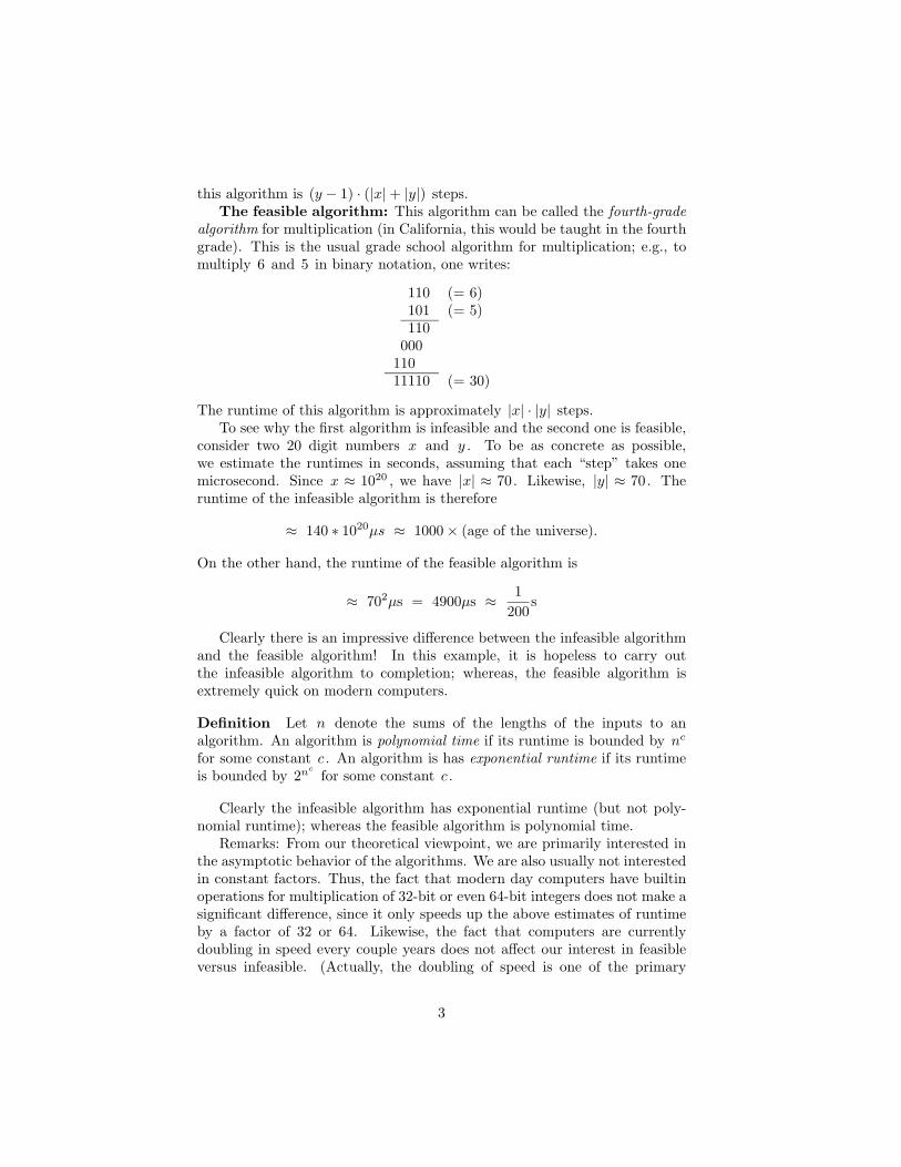
this algorithm is (y − 1) · (|x| + |y|) steps.The feasible algorithm: This algorithm can be called the fourth-grade

algorithm for multiplication (in California, this would be taught in the fourthgrade). This is the usual grade school algorithm for multiplication; e.g., tomultiply 6 and 5 in binary notation, one writes:

110 (= 6)101 (= 5)110

00011011110 (= 30)

The runtime of this algorithm is approximately |x| · |y| steps.To see why the first algorithm is infeasible and the second one is feasible,

consider two 20 digit numbers x and y . To be as concrete as possible,we estimate the runtimes in seconds, assuming that each “step” takes onemicrosecond. Since x ≈ 1020 , we have |x| ≈ 70. Likewise, |y| ≈ 70. Theruntime of the infeasible algorithm is therefore

≈ 140 ∗ 1020µs ≈ 1000 × (age of the universe).

On the other hand, the runtime of the feasible algorithm is

≈ 702µs = 4900µs ≈ 1200

s

Clearly there is an impressive difference between the infeasible algorithmand the feasible algorithm! In this example, it is hopeless to carry outthe infeasible algorithm to completion; whereas, the feasible algorithm isextremely quick on modern computers.

Definition Let n denote the sums of the lengths of the inputs to analgorithm. An algorithm is polynomial time if its runtime is bounded by nc

for some constant c . An algorithm is has exponential runtime if its runtimeis bounded by 2nc

for some constant c .

Clearly the infeasible algorithm has exponential runtime (but not poly-nomial runtime); whereas the feasible algorithm is polynomial time.

Remarks: From our theoretical viewpoint, we are primarily interested inthe asymptotic behavior of the algorithms. We are also usually not interestedin constant factors. Thus, the fact that modern day computers have builtinoperations for multiplication of 32-bit or even 64-bit integers does not make asignificant difference, since it only speeds up the above estimates of runtimeby a factor of 32 or 64. Likewise, the fact that computers are currentlydoubling in speed every couple years does not affect our interest in feasibleversus infeasible. (Actually, the doubling of speed is one of the primary

3

reasons for neglecting constant factors in runtime.)† The quadratic time,O(n2), algorithm for multiplication is not asymptotically optimal: O(n log n)runtime is possible using fast Fourier transform techniques.

1.2 P, NP, and the Polynomial-Time Hierarchy

We let N denote the set of non-negative integers.

Definition P is the set of polynomial time recognizable predicates on N .Or equivalently, P is the set of polynomial time recognizable subsets of N

FP is the set of polynomial time computable functions.

We let |x| = dlog2(x + 1)e denote the length of the binary representationof x . We write |~x|= |x1|, |x2|, . . . , |xk| .Remark: For us, functions and predicates are arithmetic: polynomial timemeans in terms of the length |x| of the input x . Generally, computerscientists use the convention that functions and predicates operate on stringsof symbols; but this is equivalent to operations on integers, if one identifiesintegers with their binary representation.

Cobham [15] defined FP as the closure of some base functions undercomposition and limited iteration on notation. As base functions, we cantake 0, S (successor), b 1

2xc , 2 · x ,

x ≤ y =

1 if x ≤ y0 otherwise

Choice(x, y, z) =

y if x > 0z otherwise

Definition Let q be a polynomial. f is defined from g and h by limitediteration on notation with space bound q iff

f(~x, 0) = g(~x)f(~x, y) = h(~x, y, f(~x, b1

2yc))

provided |f(~x, y)| ≤ q(|~x|, |y|) for all ~x, y .

Theorem 1 (Cobham [15]) FP is equal to the set of functions which canbe obtained from the above base functions by using composition and limitediteration on notation.

†The rate of increase in computing performance presently shows little sign of abating;however, if should not be expected to continue forever, since presumably physical limitswill eventually be met. It is interesting to note that if the rate of increase could besustained indefinitely, then exponential time algorithms would actually be feasible, sinceone would merely wait a polynomial amount of time for computer power to increasesufficiently to run the algorithm quickly.

4

A nondeterministic Turing machine makes “choices” or “guesses”: themachine accepts its input iff there is at least one sequence of choices thatleads to an accepting state. On the other hand, a co-nondeterministic Turingmachine makes “universal choices”: it accepts iff every possible sequence ofchoices leads to an accepting state. NP is defined to be the set of predicatesaccepted by non-deterministic polynomial time Turing machines. The classcoNP is defined to equal the set of predicates accepted by co-nondeterministicTuring machines, i.e., coNP is the set of complements of NP predicates. Forexample, the set of (codes of) satisfiable propositional formulas is in NP.And the set of (codes of) tautologies is in coNP.

We now give a second, equivalent, purely logical method of defining NPand coNP.

Definition If Ψ is a set of predicates, PB∃(Ψ) is the set of predicates Aexpressible as

~x ∈ A ⇔ (∃y ≤ 2p(|~x|))B(~x, y)

for some polynomial p and some B ∈ Ψ.PB∀(Ψ) is defined similarly with universal polynomially bounded quantifi-cation.

Definition NP = PB∃(P ) and coNP = PB∀(P ). In other words, NP isthe set of predicates A(~x) expressible in the form

A(~x) ⇔ (∃y ≤ 2p(|~x|))B(~x, y)

for some B ∈ P and some polynomial p . The class coNP is similarly definedwith a universal polynomially bounded quantifier.

Definition If Ψ is a set of predicates, PΨ (resp., FPΨ ) is the set ofpredicates (resp., functions) polynomial time recognizable with oracles for afinite number of predicates in Ψ.

The notions of P , FP , NP and coNP are generalized by defining thepolynomial time hierarchy:

Definition The Polynomial Time “Hierarchy”:

p1 = FP

∆p1 = P

Σpk = PB∃(∆p

k)Πp

k = PB∀(∆pk)

∆pk+1 = PΣp

k = PΠpk

pk+1 = FPΣp

k = FPΠpk

5

. .

. .

. .

∆p3

p3

⊆ ⊇Πp

2 Σp2

⊇⊇ ⊆

∆p2

p2

⊆ ⊇coNP = Πp

1 Σp1 = NP

⊇

⊇ ⊆P = ∆p

1p1 = FP

It is an open question whether P = NP, NP = coNP and whether thepolynomial hierarchy is proper. To sum up the current state of knowledge,all that is known is that if any two of the classes in the above hierarchy areequal, then the hierarchy collapses to those classes.

Remark: The above definitions have given purely logical characteriza-tions of the classes in the polynomial time hierarchy in terms of expressibilityin a formal language. In the next section we will give purely logicalcharacterizations of these classes in terms of derivability in a formal theory.The most important such theory is S1

2 in which the provably recursivefunctions are precisely the polynomial time computable functions. Thuswe can characterize the proof-theoretic strength of S1

2 as corresponding topolynomial time computability.

2 Bounded Arithmetic

A constructive proof system is one in which proofs of existence contain, orimply the existence of, algorithms for finding the object which is proved toexist. For a feasibly constructive system, the algorithm will be feasible, notmerely effective. For instance, if ∀x∃yA(x, y) is provable then there shouldbe a feasible algorithm to find y as a function of x . In the next section, weintroduce feasible proof systems for number theory: more precisely, S1

2 willbe a feasible proof system, and other systems, Si

2 and T i2 are systems that

have proof-theoretic strength corresponding to higher levels of the polynomialtime hierarchy.

2.1 The Language of Bounded Arithmetic

The theories of bounded arithmetic will be first-order theories for the naturalnumbers N = 0, 1, 2, . . . . The first-order language for bounded arithmeticcontains the predicates = and ≤ and contains function symbols 0, S

6

(successor), +, · , b 12xc , |x| , # and relation symbol ≤ , where

x#y = 2|x|·|y|

It is easy to check that the # (pronounced “smash”) function allows us toexpress 2q(|~a|) for q any polynomial with positive integer coefficients.

Definition A bounded quantifier is a quantifier of the form (Qx ≤ t) witht a term not involving x . A sharply bounded quantifier is one of the form(Qx ≤ |t|). (∀x) and (∃x) are unbounded quantifiers. A bounded formula isone with no unbounded quantifiers.

A hierarchy of classes Σbk , Πb

k of bounded formulas is defined by countingalternations of bounded quantifiers, ignoring sharply bounded quantifiers.(Analogously to defining the arithmetic hierarchy by counting unboundedquantifiers, ignoring bounded quantifiers.)

Definition Σb0 = Πb

0 is the set of formulas with only sharply boundedquantifiers.

If A ∈ Σbk then (∀x ≤ |t|)A and (∃x ≤ t)A are in Σb

k and (∀x ≤ t)Ais in Πb

k+1 . Dually, if A ∈ Πbk then (∃x ≤ |t|)A and (∀x ≤ t)A are in Πb

k

and (∃x ≤ t)A is in Σbk+1 . For formulas not in prenex form, we say that

a formula is in Σbi (resp., Πb

i ) iff prenex operations can be used to put theformula in to the prenex Σb

1 (resp., Πbi ) form defined above.

One of the primary justifications for the definition of Σbi - and Πb

i -formulasis the following theorem.

Theorem 2 Fix k ≥ 1 . A predicate Q is in Σpk iff there is a Σb

k formulawhich defines it.

This theorem is essentially due to Stockmeyer [48] and Wrathall [51];Kent and Hodgson [31] were the first to prove a full version of this.

Remarks: There are several reasons why the # function and sharplybounded quantifiers are natural choices for inclusion in the language ofbounded arithmetic:

• The # function has the right growth rate for polynomial timecomputation.

• The above theorem defines the Σ, Π classes of the polynomial hierarchysyntactically (without use of computation),

• The presence of # in the language gives precisely the right growth rateso that the following Quantifier Exchange Principle holds:

(∀x ≤ |a|)(∃y ≤ b)A(x, y) ↔↔ (∃y ≤ (2a + 1)#(4(2b + 1)2))(∀x ≤ |a|)

[A(x, β(x + 1, y)) ∧ β(x + 1, y) ≤ b]

7

• The original use of the # function was by E. Nelson [38]; his primaryreason for its introduction was that the growth rate of # allows asmooth treatment of sequence coding and of the metamathematics ofsubstitution. Wilkie and Paris [50] independently introduced the axiomΩ1 (“xlog x is total”) for similar reasons, since it gives similar growthrate.

The original use of polynomially bounded quantifiers was by Bennett [1];they were first defined in form given above by [3, 4].

2.2 Induction Axioms for Bounded Arithmetic

The IND axioms are the usual induction axioms. The PIND and LINDaxioms are “polynomial” and “length” induction axioms that are intendedto be feasibly effective forms of induction.

Definition Let i ≥ 0. The following are axiom schemes often used fortheories of bounded arithmetic.

Σbk -IND: A(0) ∧ (∀x)(A(x) ⊃ A(x + 1)) ⊃ (∀x)A(x) for A ∈ Σb

k .

Σbk -PIND: A(0) ∧ (∀x)(A(b1

2xc) ⊃ A(x)) ⊃ (∀x)A(x) for A ∈ Σbk .

Σbk -LIND: A(0) ∧ (∀x)(A(x) ⊃ A(x + 1)) ⊃ (∀x)A(|x|) for A ∈ Σb

k .

The axiom schemes Σbk -LIND and Σb

k -PIND typically are equivalent and are(strictly?) weaker than Σb

k -IND. Since exponentiation is not provably totalin Bounded Arithmetic, the |x| function is not provably surjective; therefore,the LIND axioms do not appear to equal to the IND axioms in strength.

2.3 Theories of Bounded Arithmetic

Definition Let i ≥ 0. T i2 is the first-order theory with language 0, S , +,

· , b 12xc , |x| , # and ≤ and axioms:

(1) A finite set, BASIC, of (universal closures of) open axioms definingsimple properties of the function and relation symbols. BASIC properlycontains Robinson’s Q since it has to be used with weaker inductionaxioms.

(2) The Σbi -IND axioms.

T−12 has no induction axioms. T2 is the union of the T i

2 ’s.

T2 is equivalent to I∆0 + Ω1 (see Parikh [40] and Wilkie and Paris [50])modulo differences in the nonlogical language.

Definition Let i ≥ 0. Si2 is the first-order theory with language 0, S , +,

· , b 12xc , |x| , # and ≤ and axioms:

8

(1) The BASIC axioms, and(2) The Σb

i -PIND axioms.

S−12 = T−1

2 has no induction axioms. S2 is the union of the Si2 ’s.

Remark: The theory S12 , which we will relate closely to polynomial

computability, is defined by PIND on NP properties (in light of Theorem 2).

The following, somewhat surprising, relationship holds between thehierarchy of theories Si

2 and the hierarchy of theories T i2 .

Theorem 3 (Buss [3, 4]). Let i ≥ 1 . T i2 ` Si

2 and Si2 ` T i−1

2 . So S2 ≡ T2 .

Open Question: Are the following inclusions proper?

S12 ⊆ T 1

2 ⊆ S22 ⊆ T 2

2 ⊆ · · ·

2.4 Provably Recursive and Σbi -Definable Functions

We know come to one of the centrally important definitions for describingthe proof-theoretic complexity of bounded arithmetic:

Definition Let f :Nk 7→ N . The function f is Σbi -definable by a theory R

iff there is a formula A(~x, y) ∈ Σbi so that

(1) For all ~n ∈ Nk , A(~n, f(~n)) is true.

(2) R ` (∀~x)(∃y)A(~x, y)

(3) R ` (∀~x, y, z)(A(~x, y) ∧ A(~x, z) ⊃ y = z)

When a function is Σb1 -definable by a theory R , then we also say that the

function is provably recursive in R . By “provably recursive” we are intendingthat there should be a Turing machine M which computes the function sothat R can prove the Turing machine always halts within polynomial time.By a “bootstrapping procedure” it is possible to show that, for a givenTuring machine M and a given polynomial time bound p(n), the statementthat M always halts within time p(|x|) can be expressed in the form(∀x)(AM,p(x)) where AM,p is a Σb

1 -formula. (Actually, this fact is immediatefrom Theorem 2, so no further bootstrapping is needed.) On the other hand,any Σb

1 -definable function is certainly Turing computable; it can be computedby a (non-polynomial time) brute-force search if nothing else. Therefore, itmakes sense to identify “provably recursive” and “Σb

1 -definable”.The concept of Σb

i -definability applies to functions only. The analoguefor predicates is the notion of ∆b

i -definability:

Definition Let Q ⊆ N . Q is ∆bi -definable by a theory R iff there is

a Σbi -formula A and Πb

i -formula B that define Q so that A and B areprovably equivalent in R . A formula is ∆b

i with respect to R iff it isprovably equivalent to a Σb

i - and to a Πbi -formula.

9

2.5 Bootstrapping Theorems

Theorem 4 [3, 4] Every polynomial time function is Σb1 -definable by S1

2

and every polynomial time predicate is ∆b1 -definable by S1

2 .

The above theorem shows that S12 , and the Σb

i -definable functions and∆b

1 -definable predicates are sufficiently strong to introduce polynomial timeproperties. We will omit the proof of this theorem here: for details, thereader can refer to Buss [3, 4], some improvements to the bootstrapping canbe found in Buss-Ignjatovic [13] and a proof outline can be found in [7].Alternative approaches to bootstrapping in different settings are given byWilkie-Paris [50] and in Hajek-Pudlak [25].

A large part of the importance of Σb1 -definable functions and ∆b

1 -predicates comes from the following theorem:

Theorem 5 [3, 4] Let i ≥ 1 . Any Σb1 -definable function or ∆b

1 -definablepredicate of Si

2 may be introduced into the nonlogical language and used freelyin induction axioms. The same holds for T i

2 in place of Si2 .

Proof (Sketch) Suppose f is Σb1 -defined by R , so that

R ` (∀x)(∃!y ≤ r(~x))Af (~x, y).

Then any atomic formula ϕ(f(~s)) is equivalent to both

(∃y ≤ r(~s))(Af (~s, y) ∧ ϕ(y))

and(∀y ≤ r(~s))(Af (~s, y) ⊃ ϕ(y)).

Note that the first formula is in Σbi and the second is in Πb

i . Thus, fori odd, any Σb

i -formula involving f is equivalent to one not involving f bytransforming atomic subformulas as above using the first equivalent formulafor positively occurring subformulas and the second equivalent formula fornegatively occurring subformulas. For i even, the roles of positive andnegative occurrences are reversed. (We have omitted some details from thisproof, since it is also necessary to remove f from terms in quantifier bounds;this is possible because of the known bound r(~x) on the value of f(~x).) 2

2.6 Main Theorems for Si2

The so-called “main theorems” for the theories Si2 give an exact character-

ization of the Σbi -definable functions of Si

2 in terms of the computationalcomplexity.

10

Theorem 6 (Buss [3, 4]) Let i ≥ 1 . Let A be a Σbi -formula. Suppose

Si2 ` (∀~x)(∃y)A(~x, y) . Then there is a Σb

i -formula B and a function f ∈ pi

and a term t so that

(1) Si2 ` (∀~x, y)(B(~x, y) ⊃ A(~x, y)) .

(2) Si2 ` (∀~x)(∃!y)B(~x, y) .

(3) Si2 ` (∀~x)(∃y ≤ t)B(~x, y) . (see Parikh [40])

(4) For all ~n , N |= B(~n, f(~n)) .

Theorem 7 If f ∈ pi then there is a formula B ∈ Σb

i and a term t so that(2), (3) and (4) hold.

Corollary 8 (i ≥ 1) The Σbi -definable functions of Si

2 are precisely thefunctions in p

i .

The most interesting case of the above theorems and corollary is probablythe i = 1 case. For this, we have:

Corollary 9 The Σb1 -definable functions of S1

2 are precisely the polynomialtime functions.

It is this corollary that allows us to state that the proof-theoretic strengthof S1

2 corresponds to polynomial time computability.The above theorems characterize the Σb

i -definable functions of Si2 . These

can be restated to characterize the ∆bi -definable predicates of Si

2 .

Definition A predicate Q(~x) is ∆bi -definable in a theory T provided it is

defined by a Σbi -formula A(~x) and a Πb

i -formula B(~x) such that T proves(∀~x)(A(~x) ↔ B(~x)).

Theorem 10 (i ≥ 1). Suppose A(~x) ∈ Σbi and B(~x) ∈ Πb

i and Si2 ` A ↔

B . Then there is a predicate Q ∈ ∆pi so that, for all ~n ,

Q(~n) ⇔ N |= A(~n) ⇔ N |= B(~n)

Conversely, if Q ∈ ∆pi then there are A and B so that the above holds.

In other words, the ∆bi -definable predicates of Si

2 are precisely the ∆pi -

predicates.

The most interesting case of the last theorem is again probably the i = 1case. For this, we have:

Corollary 11 If A is a formula which is S12 -provably in NP ∩ coNP then

A defines a polynomial time predicate (provably in S12 ). Being provably in

NP ∩ coNP means provably equivalent to a Σb1 - and to a Πb

1 -formula.

11

We shall sketch a proof of the main theorem below; but first, we need totake a diversion into the sequent calculus. The sequent calculus and the cutelimination theorem will be one of the main tools in our proof of the maintheorems.

3 The Sequent Calculus

3.1 Gentzen’s Sequent Calculus

To prove the Main Theorem, we shall formalize Si2 in Gentzen’s sequent

calculus.We shall work in first-order logic with ∧ , ∨ , ¬ , ⊃ , ∀ , ∃ the logical

symbols of our first language. In addition, there is one further symbol, → ,which is the sequent connective. The sequent connective does not occurin first-order formulas per se, but instead is used to mark the middle of asequent:

Definition A sequent is an expression of the form

A1, A2, . . . , An→B1, B2, . . . , Bk

where the Ai ’s and Bi ’s are formulas. Its intended meaning is

(A1 ∧ A2 ∧ · · · ∧ An) ⊃ (B1 ∨ B2 ∨ · · · ∨ Bk)

We shall use Greek letters Γ,∆, . . . to denote finite sequences of formulasseparated by commas. A sequent is thus denoted Γ→∆. The cedents Γand ∆ are called the antecedent and succedent of the sequent (respectively).

Gentzen’s sequent calculus is a proof system where lines in the proofsare sequents. The sequent calculus is generally denoted LK , from “LogischeKalkul”.

Definition An LK-proof is a tree of sequents: the leaves or initial sequentsmust be of the form A→A ; the root, or endsequent, is what is proved; andthe valid inferences are:

Γ→ ∆, A

¬A,Γ→ ,∆A,Γ→ ∆

Γ→ ∆,¬A

A,Γ→ ∆A ∧ B,Γ→ ∆

Γ→ ∆, A Γ→ ∆, B

Γ→ ∆, A ∧ B

B,Γ→ ∆A ∧ B,Γ→ ∆

Γ→ ∆, A

Γ→ ∆, A ∨ B

A,Γ→ ∆ B,Γ→ ∆A ∨ B,Γ→ ∆

Γ→ ∆, B

Γ→ ∆, A ∨ B

12

Γ→ ∆, A B,Γ→ ∆A ⊃ B,Γ→ ∆

A,Γ→ ∆, B

Γ→ ∆, A ⊃ B

A(b),Γ→ ∆(∃x)A(x),Γ→ ∆

Γ→ ∆, A(t)Γ→ ∆, (∃x)A(x)

A(t),Γ→ ∆(∀x)A(x),Γ→ ∆

Γ→ ∆, A(b)Γ→ ∆, (∀x)A(x)

In the quantifier inferences, the free variable b is called the eigenvariable andmust not appear in the lower sequent.

Γ→ ∆A,Γ→ ∆

Γ→ ∆Γ→ ∆, A

Γ, A,B,Π→ ∆Γ, B,A,Π→ ∆

Γ→ ∆, A,B,ΛΓ→ ∆, B,A,Λ

A,A,Γ→ ∆A,Γ→ ∆

Γ→ ∆, A,A

Γ→ ∆, A

Cut:Γ→ ∆, A A,Π→ Λ

Γ,Π→ ∆,Λ

The system LK , as defined above, gives a sound and complete proofsystem for first-order logic. It is probably the most elegant way offormulating first-order logic; and a primary factor in its elegance is thefollowing fundamental theorem:

Theorem 12 (Gentzen [23])

• LK is complete.

• LK without the Cut inference is complete.

In particular, if P is an LK-proof of Γ→∆ then there is a cut-free proofP ∗ of Γ→∆. There is an effective (but not feasible) procedure to obtainP ∗ from P .

Examination of the rules of inference for LK reveals that, with theexception of the cut rule, every inference has the subformula property thatthe formulas in the hypotheses of the inference are subformulas of formulasin the conclusion (the lower sequent) of the inference. More precisely, everyformula in the upper sequents is obtained from a subformula of a formulain the lower sequent, possibly after substitution of a term for a (formerly)bound variable. In other words, every formula in an upper sequent is asubformula in the wide sense of some formula in the lower sequent.

Thus, if there are no cuts, the logical complexity of formulas in the proofwill be at most the logical complexity of formulas in the endsequent Γ→∆.We therefore say that cut-free sequent calculus proofs enjoy the subformulaproperty.

13

3.2 Sequent Calculus Formulations of BoundedArithmetic

We now wish to formulate a sequent calculus version of the theories ofbounded arithmetic in a way that preserves the essence of the this subformulaproperty. We there for enlarge LK as follows:

(1) Allow equality axioms and BASIC axioms as initial sequents. An initialsequent will contain only atomic formulas.

(2) Add inferences for bounded quantifiers (the variable b occurs only asindicated):

b ≤ s,A(b),Γ→ ∆(∃x ≤ s)A(x),Γ→ ∆

Γ→ ∆, A(t)t ≤ s,Γ→ ∆, (∃x ≤ s)A(x)

A(t),Γ→ ∆t ≤ s, (∀x ≤ s)A(x),Γ→ ∆

b ≤ s,Γ→ ∆, A(b)Γ→ ∆, (∀x ≤ s)A(x)

(3) Allow induction inferences: (for A ∈ Σbi )

Σbi -IND

A(b),Γ→ ∆, A(b + 1)A(0),Γ→ ∆, A(t)

Σbi -PIND

A(b 12bc),Γ→ ∆, A(b)

A(0),Γ→ ∆, A(t)

Definition Si2 and T i

2 are formulated as sequent calculus systems withBASIC axioms as initial sequents and with Σb

i -PIND and Σbi -IND inference

rules, respectively. With side formulas, the induction inferences areequivalent to the induction axioms.

3.3 Free-Cut Elimination

Definition A cut inference

Γ→ ∆, A A,Π→ ΛΓ,Π→ ∆,Λ

is free unless A is the direct descendant either of a formula in an initialsequent or of a principal formula of an induction inference.

The next theorem is due to Gentzen and Takeuti (for fragments of Peanoarithmetic).

14

Theorem 13 Free-Cut Elimination Theorem If P is an Si2 -proof (or

T i2 -proof) then there is a proof P ∗ in the same theory with the same endsequent

which contains no free cuts.

In a free-cut free proof, every formula will be a subformula (in the widesense) of an induction formula, of a formula in an axiom or of a formula inthe conclusion.

In Si2 and T i

2 , cut formulas may be restricted to be Σbi -formulas.

Therefore, if Γ→∆ is a sequent of Σbi -formulas which is a consequence

of Si2 or T i

2 , then Γ→∆ has an Si2 -proof or T i

2 -proof (respectively) suchthat every formula appearing in the proof is in Σb

i .

3.4 Outline of Proof of the Main Theorem

There are two steps in the proof of Theorem 6Step 1: By assumption, there is an Si

2 -proof P of

→(∃y)A(~c, y).

Therefore, by free-cut elimination, there is an Si2 proof P ∗ of

→(∃y ≤ t)A(~c, y)

such that every formula in P ∗ is a Σbi -formula.

Step 2: Given the proof P ∗ we will extract an algorithm to computea function f(~c) such that A(~n, f(~n)) is true for all n . The function fwill be in p

i and will be Σbi -defined by Si

2 . Furthermore, Si2 will prove

(∀~x)A(~x, f(~x)). Thus, P ∗ can be thought of as a program plus a proof thatit is correct.

Step 1 is immediate from the free-cut elimination theorem. Before, wecan carry out Step 2, we need to introduce the Witness predicate.

3.5 The Witness Predicate

Definition Fix i ≥ 1. Let B(~a) be a Σbi -formula with all free variables

indicated. Then Witnessi,~aB (w,~a) is a formula defined inductively by:

(1) If B ∈ Σbi−1 ∪ Πb

i−1 then Witnessi,~aB (w,~a) ⇔ B(~a).

(2) If B = C ∨ D then

Witnessi,~aB (w,~a) ⇔ Witnessi,~a

C (β(1, w),~a) ∨ Witnessi,~aD (β(2, w),~a).

(3) If B = C ∧ D then

Witnessi,~aB (w,~a) ⇔ Witnessi,~a

C (β(1, w),~a) ∧ Witnessi,~aD (β(2, w),~a).

15

(4) If B = (∃x ≤ t)C(~a, x) then

Witnessi,~aB (w,~a) ⇔ β(1, w) ≤ t ∧ Witnessi,~a,b

C(~a,b)(β(2, w),~a, β(1, w)).

(5) If B = (∀x ≤ |t|)C(~a, x) then

Witnessi,~aB (w,~a) ⇔ (∀x ≤ |t|)Witnessi,~a,b

C(~a,b)(β(x + 1, w),~a, x).

(6) If B = ¬C use prenex operations to push the negation sign inside.

Lemma 14 Fix i ≥ 1 . Let B ∈ Σbi .

(1) For some term tB , Si2 proves

B(~a) ↔ (∃w ≤ tB)Witnessi,~aB (w,~a).

(2) Witnessi,~aB ∈ ∆p

i (= P if i = 1).

(3) Witnessi,~aB is ∆b

i with respect to Si2 .

Proof: This is easily proved by induction on the complexity of B .

3.6 The Main Lemma

Lemma 15 Suppose Si2 ` Γ→∆ where Γ and ∆ contain only Σb

i -formulas.Let ~c be the free variables in Γ and ∆ . Then, there is a function f such that

(a) f is Σbi -defined by Si

2

(b) Si2 ` Witnessi,~c∧∧

Γ(w,~c) ⊃ Witnessi,~c∨∨∆(f(w,~c),~c)

(c) f ∈ pi (= FP if i = 1)

Proof The proof is by induction on the number of inferences in a free-cutfree Si

2 -proof of Γ→∆. As an example of one case of the proof of the mainlemma, suppose that P is a free-cut free proof and ends with the inference

B(b 12ac)→ B(a)

B(0)→ B(t)

By the induction hypothesis, there is a function g so that

(1) g is Σbi -defined by Si

2

(2) g is in pi (= FP if i = 1)

(3) Si2 ` Witnessi,a,~c

B(b 12ac)

(w, a,~c) ⊃ Witnessi,a,~cB(a)(g(w, a,~c), a,~c).

16

(4) Si2 ` (∀a,~c)[g(w, a,~c) ≤ tB(a,~c)]

Now define f by limited iteration as

f(w, 0,~c) = g(w, 0,~c)f(w, a,~c) = g(f(w, b 1

2ac,~c), a,~c)

so f(w, a,~c) ≤ tB(a,~c) and the following hold:

(1) f ∈ pi (= FP if i = 1)

Pf: Since f is defined by limited iteration from g .

(2) Si2 can Σb

i -define f and prove that f satisfies the above conditions

(3) Si2 ` Witnessi,a,~c

B(0,~c)(w, a,~c) ⊃ Witnessi,a,~cB(a,~c)(f(w, a,~c), a,~c).

Pf: Since Witnessi,b,~cB(a,~c) is a Σb

i -formula, Si2 can prove this by Σb

i -PINDdirectly from the induction hypothesis.

Q.E.D. Main Lemma 15

3.7 Conclusion of Proof of Main Theorem

We can now prove the Main Theorem 6 for Si2 from the above Lemma 15.

Proof Suppose Si2 ` (∀~x)(∃y)A(~x, y). By a theorem of Parikh, there is a

term t so that Si2 proves →(∃y ≤ t)A(~c, y) . By the Main Lemma,

Si2 ` Witnessi,~c

(∃y≤t)A(g(~c),~c)

for some Σbi -defined function g . Define B(~c, y) to be the formula

y = β(1, g(~c)).

Since g is Σbi -defined by Si

2 , B is a Σbi -formula and by the properties of

Witness,Si

2 ` (∀~x, y)(B(~x, y) ⊃ A(~x, y))

Finally, define f(~c) = β(1, g(~c)).Q.E.D. Main Theorem 6

4 Other Systems of Bounded Arithmetic

4.1 Alternative Axioms for Bounded Arithmetic

Let Ψ be a set of formulas. The axioms below are schemes where A ∈ Ψ:

17

Ψ-MIN: (Minimization)

(∃x)A(x) ⊃ (∃x)[A(x) ∧ (∀y < x)(¬A(y))]

Ψ-LMIN: (Length minimization)

(∃x)A(x) ⊃ A(0) ∨ (∃x)[A(x) ∧ (∀y ≤ b 12xc)(¬A(y))]

Ψ-replacement:

(∀x ≤ |t|)(∃y ≤ s)A(x, y) ↔↔ (∃w ≤ SqBd(t, s))(∀x ≤ |t|)(A(x, β(Sx,w)) ∧ β(Sx,w) ≤ s)

strong Ψ-replacement:

(∃w ≤ SqBd(t, s))(∀x ≤ |t|)[(∃y ≤ s)A(x, y) ↔ A(x, β(Sx,w)) ∧ β(Sx,w) ≤ s]

The figure below shows the known relationships between fragments ofbounded arithmetic: (for i ≥ 1, relative to S1

2 )

Σbi -IND ⇔ Πb

i -IND ⇔ Σbi -MIN ⇔ ∆b

i+1-INDwwÄΣb

i -PIND ⇔ Πbi -PIND ⇔ Σb

i -LIND ⇔ Πbi -LIND~wÄ

Σbi -LMIN ⇔ strong Σb

i -replacementwwÄ ~wÄΣb

i−1-IND (Σbi+1 ∩ Πb

i+1)-PIND

Σbi+1-MIN ⇔ Πb

i -MIN

Σbi+1-replacement ⇒ Σb

i -PIND ⇒ Σbi -replacement

Si+12 Â

Σbi+1

T i2

Si+12 Â

B(Σbi+1)

T i2 + Σb

i+1-replacement

Due to space limitations, we shall only sketch proofs of two of the factspictured in the above figure.

Theorem 16 [3, 4] S12 + Σb

i -PIND ` ∆bi -IND . Hence Si

2 ⊃ T i−12 .

18

Proof Suppose A is ∆bi w.r.t. Si

2 . Assume (∀x)(A(x) ⊃ A(x + 1)) andargue inside Si

2 . Let B(x, z) be the formula

(∀w ≤ x)(∀y ≤ z + 1)(A(w .− y) ⊃ A(w)).

So B is equivalent to a Πbi -formula. Now by definition of B ,

(∀x, z)(B(x, b 12zc) ⊃ B(x, z)) and hence by Πb

i -PIND on B(x, z) w.r.t. z ,

(∀x)(B(x, 0) ⊃ B(x, x)).

By the assumption, (∀x)B(x, 0); hence (∀x)B(x, x), from whence

(∀x)(A(0) ⊃ A(x)) 2

The second result is concerns the conservation results between T i2 and

Si+12 :

Theorem 17 [8] Fix i ≥ 1 . Si+12 is conservative over T i

2 with respect toΣb

i+1 -formulas, and hence with respect to ∀∃Σbi+1 -sentences.

This means that any ∀∃Σbi+1 -formula which is Si+1

2 -provable is alsoT i

2 -provable.

Proof (Idea). Fix i ≥ 1 and let Z be PV or T i−12 as appropriate. First

show that every pi -function is definable in Z in an appropriate sense.

For i = 1, there is a function symbol for every polynomial time function;for i > 1, we show that every p

i -function can be “Qi -defined” — this isstronger than “Σb

i -defined”. Second, prove a stronger version of the MainLemma above; in essence, we partially formalize the Main Lemma in Z andprove that the witnessing function f is defined appropriately in Z . Namely,we prove that if Si

2 ` A with A ∈ Σbi then Z ` A .

We omit the rest of the proof details.

A nice consequence of the previous theorem and of the Main Theoremfor Si

2 is:

Theorem 18 [8] The Σbi+1 -definable theories of T i

2 are precisely the pi+1 -

functions.

4.2 Witnessing Theorem for T 12

The class Polynomial Local Search, PLS, was defined by Papadimitriou [39]to capture a common kind of search problem. Two representative examplesof PLS problems are (1) linear programming and (2) simulated annealing.Of course, it is known that there are polynomial time algorithms for linearprogramming. On the other hand, there is no polynomial time algorithmwhich is known to find even a local optimum solution based on simulatedannealing. So, it is open whether PLS is in P .

19

Definition A Polynomial Local Search (PLS), problem is specified by twopolynomial time functions N, c and a polynomial time predicate F whichsatisfy the following conditions:

(1) c(s, x) is a cost function,

(2) N(s, x) is a neighborhood function, such that for all s such that F (s, x)holds, we have

c(N(s, x), x) ≤ c(s, x) and F (N(s, x), x).

(3) s : F (s, x) is the solution space for input x . F (0, x) always holds;and if F (s, x), then |s| < p(|x|) for p some polynomial.

A solution to the PLS problem is a (multivalued) function f , s.t., for all x ,

c(N(f(x), s), s) = c(f(x), x) and F (f(x), x).

Theorem 19 [14] Suppose T 12 proves (∀x)(∃y)A(x, y) where A ∈ Σb

1 . Thenthere is a PLS function f(x) = y and a polynomial time function π such that

T 12 ` (∀x)A(x, π f(x)).

Furthermore, every PLS function (and every function π f ) is Σb1 -definable

by T 12 .

Corollary 20 The same holds for S22 by conservativity of S2

2 over T 12 .

Proof-idea: A free-cut free T 12 -proof can be transformed into a PLS

problem. 2

4.3 Herbrand’s Theorem and the KPT WitnessingTheorem

The following theorem is a version of Herbrand’s Theorem from Herbrand’sdissertation [27, 30, 28]. A proof of (a strengthening of) this version ofHerbrand’s theorem can be found in [10].

Theorem 21 Let T be a theory axiomatized by purely universal axioms. LetA(x, y, z) be quantifier-free. Suppose T proves

(∀x)(∃y)(∀z)A(x, y, z).

Then there is an integer k > 0 and there are terms t1(x) , t2(x, z1) ,t3(x, z1, z2), . . . , tk(x, z1, . . . , zk−1) so that:

T ` (∀x)[(∀z1)[A(x, t1(x), z1)∨(∀z2)[A(x, t2(x, z1), z2) ∨(∀z3)[A(x, t3(x, z1, z2), z3) ∨

...(∀zk)[A(x, tk(x, z1, . . . , zk−1), zk)] · · ·]]].

20

The KPT Witnessing Theorem (Theorem 22 below) applies this theoremto the theories T i

2 . In order to do this, however, we must re-axiomatize T i2

to have purely universal axioms. In order to give a set of purely universalaxioms, we must enlarge the language of T i

2 by adding function symbols allpi+1 -functions. Of course, we want to have only a conservative extension

of T i2 when we enlarge the language: By Theorem 18, T i

2 can alreadyΣb

i+1 -define all bi+1 functions; therefore, we can add symbols for these

functions to the language of T i2 and add the defining equations for these new

function symbols and still have a conservative extension of T i2 .

Towards this end, we define:

Definition Let i ≥ 1. The theory PVi = T i2(

pi+1) is defined to be

the theory T i2 with language enlarged to include function symbols for all

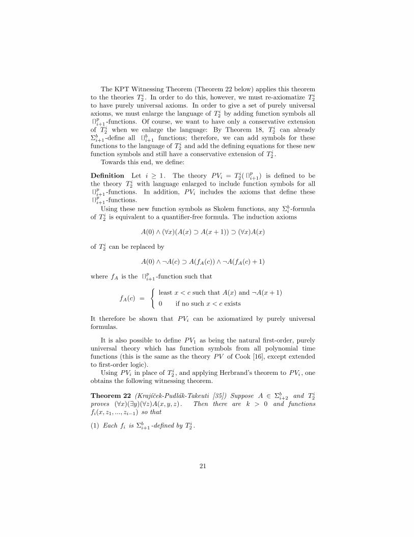
pi+1 -functions. In addition, PVi includes the axioms that define thesepi+1 -functions.Using these new function symbols as Skolem functions, any Σb

i -formulaof T i

2 is equivalent to a quantifier-free formula. The induction axioms

A(0) ∧ (∀x)(A(x) ⊃ A(x + 1)) ⊃ (∀x)A(x)

of T i2 can be replaced by

A(0) ∧ ¬A(c) ⊃ A(fA(c)) ∧ ¬A(fA(c) + 1)

where fA is the pi+1 -function such that

fA(c) =

least x < c such that A(x) and ¬A(x + 1)

0 if no such x < c exists

It therefore be shown that PVi can be axiomatized by purely universalformulas.

It is also possible to define PV1 as being the natural first-order, purelyuniversal theory which has function symbols from all polynomial timefunctions (this is the same as the theory PV of Cook [16], except extendedto first-order logic).

Using PVi in place of T i2 , and applying Herbrand’s theorem to PVi , one

obtains the following witnessing theorem.

Theorem 22 (Krajıcek-Pudlak-Takeuti [35]) Suppose A ∈ Σbi+2 and T i

2

proves (∀x)(∃y)(∀z)A(x, y, z) . Then there are k > 0 and functionsfi(x, z1, ..., zi−1) so that

(1) Each fi is Σbi+1 -defined by T i

2 .

21

(2) T i2 proves

(∀x)[(∀z1)[A(x, f1(x), z1)∨(∀z2)[A(x, f2(x, z1), z2) ∨(∀z3)[A(x, f3(x, z1, z2), z3) ∨

...(∀zk)[A(x, fk(x, z1, . . . , zk−1), zk)] · · ·]]].

4.4 Collapse of the Polynomial Hierarchy

As mentioned earlier, it is open whether the hierarchy of theories of boundedarithmetic is proper. Because of the close relationship between the fragmentsof bounded arithmetic and the levels of the polynomial time hierarchy, itis natural to try to find a connection between the questions of whetherthese two hierarchies are proper. This is answered by the following theorem,which shows that the hierarchy of theories of bounded arithmetic collapsesif and only if bounded arithmetic is able to prove that the polynomial timehierarchy is proper.

Theorem 23 (Krajıcek-Pudlak-Takeuti [35], Buss [11], Zambella [52])If T i

2 = Si+12 , then the polynomial time hierarchy collapses, provably in T i

2 .In fact, in this case, T i

2 proves that every Σpi+3 predicate is (a) equivalent to

a Boolean combination of Σpi+2 -predicates and (b) is in Σp

i+1/poly .

Proof (Idea) For simplicity, assume i = 0. Suppose T 02 (PV ) = S1

2 . Letϕ represent a vector of Boolean formula ϕ = 〈ϕ1, . . . , ϕn〉 . Then T 0

2 (PV )proves

∀ϕ(∃` ≤ n)(∃〈w1, . . . , w`〉)[(∀j ≤ `)(wj satisfies ϕj) ∧ “` = n or ϕ`+1 is unsatisfiable”]

The formula in [· · ·] is in Πb1 , so the KPT witnessing theorem can be applied

to get k > 0 and polynomial time functions f1, . . . , fk so that T 02 (PV )

proves (setting n = k ) that given ϕ1, . . . , ϕk satisfied by w1, . . . wk , thatone of fj(ϕ,w1, . . . , wj−1) produces a witness to ϕj . [Note that fj has allϕi ’s as input.]

Let PreAdvice(a, 〈ϕ`+1, . . . , ϕk〉) mean that for all ϕ1, . . . , ϕ` < asatisfied by w1, . . . , w` , fj(ϕ,w1, . . . , wj−1) satisfies ϕj for some j ≤ ` .Let Advice(a, 〈ϕ`+1, . . . , ϕk〉) mean that PreAdvice holds, and that ` is theminimum possible value for which there is such PreAdvice.

Claim T 02 (PV ) proves, that if ϕ` < a and if Advice(a, 〈ϕ`+1, . . . , ϕk〉),

then ϕ` is satisfiable if and only if for all ϕ1, . . . , ϕ` , satisfied by w1, . . . , w` ,there is j ≤ ` such that fj(ϕ,w1, . . . , wj−1) satisfies ϕj .

22

Proof of claim: If the latter condition is true, then the only way for〈ϕ`, . . . , ϕk〉 to not be “preadvice”, (which it isn’t, by definition of “advice”)is for ϕ` to be satisfied by f`(ϕ, ~w) for some ϕ1, . . . , ϕ`−1 , w1, . . . , w`−1 . 2

Note that this means that the NP complete property of satisfiability isin coNP relative to the polynomial size advice, 〈ϕ`, . . . , ϕk〉 .

The above shows that T 02 (PV ) would prove NP ⊆ coNP/poly . From this,

Karp-Lipton style methods can show that T 02 (PV ) proves the polynomial

time hierarchy collapses. In fact it can be shown that T 02 (PV ) proves

that every polynomial time hierarchy predicate is equivalent to Booleancombination of Σp

2 predicates. The proof idea is that the property PreAdviceis in coNP and therefore, property

PAlen(`) ≡ ∃〈ϕ`+1, . . . , ϕk〉PreAdvice(a, 〈~ϕ〉)is a Σp

2 -property.Similar methods work for i ≥ 1. Q.E.D.

5 Lengths of Propositional Proofs

5.1 Frege and Extended Frege Systems

Definition Propositional Formulas are formed with logical connectives ∧ ,∨ , ¬ and ⊃ , variables p1, p2, . . . , and parentheses.

Cook’s Theorem: P = NP if and only if there is a polynomial timealgorithm for determining if a propositional formula is valid.

Frege systems are the usual “textbook” proof systems for propositionallogic:

Definition A Frege (F ) proof system is a usual proof system forpropositional logic with a finite set of axiom schemes and with only themodus ponens rule. F is sound and complete.

Open Question: Does every tautology have a polynomial size F -proof?

If the answer to this question is “Yes”, then NP=coNP. This is since theset of tautologies is coNP complete and having a polynomial size F -proof isan NP property.

The size of Frege proofs is measured in terms of the number of symbolsoccurring in the proof. Of course, the number of symbols may be large eitherbecause there are a lot of steps in the proof, or because the formulas whichoccur in the proof are large. In the latter case, there will generally be manyrepeated subformulas; this motivates the definition of “extended Frege proofsystems” where repeated subformulas may be abbreviated by new symbols.

23

Definition The extended Frege (eF ) proof system is a Frege proof systemplus the extension rule:Extension Rule: whenever q is a variable which has not been used in theproof so far and does not appear in the final line of the proof or in ϕ thenwe may infer

q ↔ ϕ.

This allows us to use q as abbreviation for ϕ . By iterating uses of extensionrule the extension rule can apparently make proofs logarithmically smallerby reducing the formula size.

Tseıtin [49] first used the extension rule, for resolution proofs. See alsoStatman [47] and Cook-Reckhow [18, 19]. Statman proved that the numberof symbols in an extended Frege proof can be polynomially bounded in termson the number of steps in the proof.

Theorem 24 Reckhow [45] The choice of axiom schemas or of logicallanguage does not affect the lengths of F - or eF -proofs by more than apolynomial amount.

5.2 Abstract Proof Systems

The following definition of propositional proof system is due to Cook [16]:

Definition A propositional proof system is a polynomial time function fwith range equal to the set of all valid formulas.

An (extended) Frege proof system can be viewed as a propositional proofsystem by letting f(w) equal the last line of w if w is a valid (e)F -proof.Similarly, any theory (e.g. set theory) can be viewed as a propositional proofsystem. For instance, ZF serves a proof system by letting f(w) be definedso that if w codes a ZF -proof that ϕ is a tautology, then f(w) equals (thecode for) ϕ .

Theorem 25 (Cook [16]) NP = coNP if and only if there is a proof system ffor which tautologies have polynomial size proofs.

To prove this theorem, note that if f is such a proof system, then thena formula is a tautology iff it has a proof of polynomial length. Therefore,the coNP complete property of being a tautology would be in NP, so NPwould equal coNP. Conversely, an NP algorithm can be turned into a proofsystem, by letting its accepting computations serve as proofs.

Definition A proof system f in which all tautologies have polynomial sizeproof is called super.

It is open whether there exist super proof systems.

24

Definition Let S and T be proof systems (with the same propositionallanguage). S simulates T iff there is a polynomial p so that for anyT -proof of size n there is an S -proof of the same formula of size ≤ p(n). Sp-simulates T iff the S -proof is obtainable as a polynomial time function ofthe T -proof.

Open Question: Does F simulate eF ?

This open question is related to the question of whether Boolean circuitshave equivalent polynomial size formulas. By Ladner [36] and Buss [5] thisis a non-uniform version of the open question of whether P is equal toalternating logarithmic time (ALOGTIME).

Open Question: Is there a maximal proof system which simulates all otherpropositional proof systems?

Krajıcek and Pudlak [33] have shown that if NEXP (non-deterministicexponential time) is closed under complements then the answer is “Yes”.

5.3 The Propositional Pigeonhole Principle

We now introduce tautologies that express the pigeonhole principle.

Definition The propositional pigeonhole principle PHPn is the formula∧0≤i≤n

∨0≤j<n

pi,j ⊃∨

0≤i<m≤n

∨0≤j<n

(pi,j ∧ pm,j)

states that n + 1 pigeons can’t fit singly into n holes. pi,j means “pigeon iis in hole j ”.

Theorem 26 (Cook-Reckhow [18, 19]) There are polynomial size eF -proofsof PHPn .

Theorem 27 ([6]) There are polynomial size F -proofs of PHPn .

Theorem 28 (Haken [26]) The shortest resolution proofs of PHPn are ofexponential size.

Cook and Reckhow had proposed PHPn as an example for showing thatF could not simulate eF . However, Theorem 27 implies this is not the case.Presently there are no very good candidates of combinatorial principles thatmight separate F from eF ; the paper [2] describes some attempts to findsuch combinatorial principles.

25

5.4 PHPn has Polysize eF -Proofs

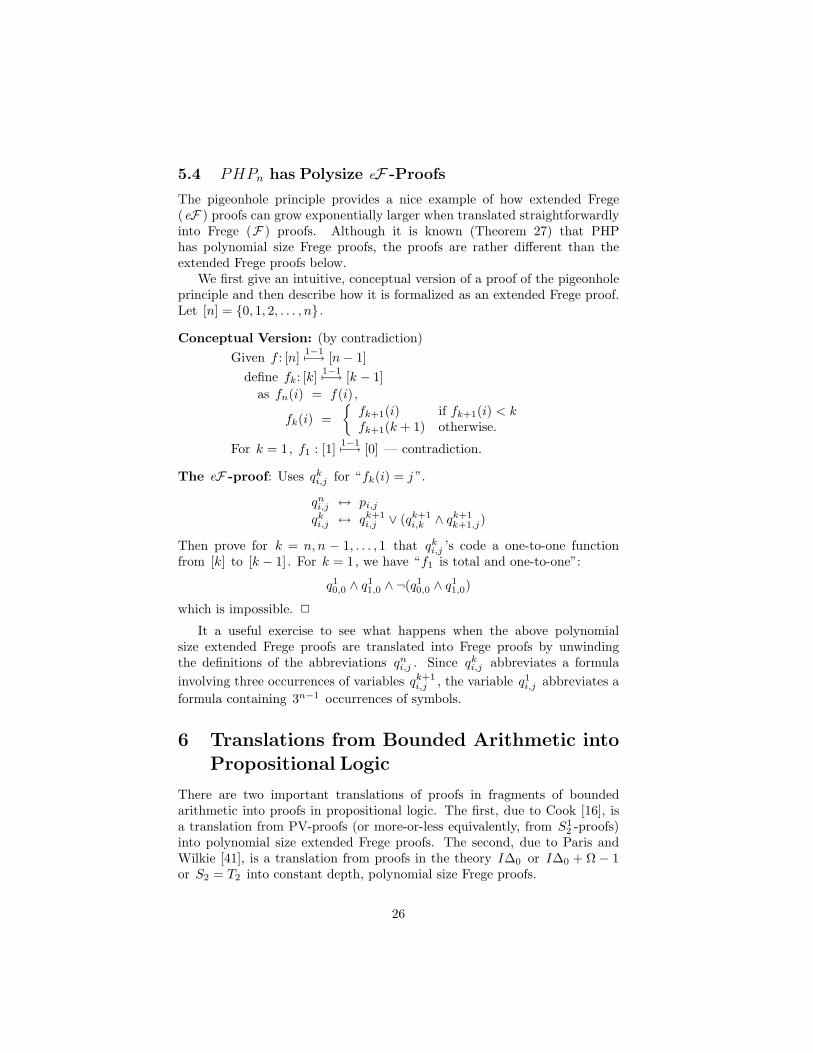
The pigeonhole principle provides a nice example of how extended Frege(eF ) proofs can grow exponentially larger when translated straightforwardlyinto Frege (F ) proofs. Although it is known (Theorem 27) that PHPhas polynomial size Frege proofs, the proofs are rather different than theextended Frege proofs below.

We first give an intuitive, conceptual version of a proof of the pigeonholeprinciple and then describe how it is formalized as an extended Frege proof.Let [n] = 0, 1, 2, . . . , n .

Conceptual Version: (by contradiction)Given f : [n] 1−17−→ [n − 1]

define fk: [k] 1−17−→ [k − 1]as fn(i) = f(i),

fk(i) =

fk+1(i) if fk+1(i) < kfk+1(k + 1) otherwise.

For k = 1, f1 : [1] 1−17−→ [0] — contradiction.

The eF -proof: Uses qki,j for “fk(i) = j ”.

qni,j ↔ pi,j

qki,j ↔ qk+1

i,j ∨ (qk+1i,k ∧ qk+1

k+1,j)

Then prove for k = n, n − 1, . . . , 1 that qki,j ’s code a one-to-one function

from [k] to [k − 1]. For k = 1, we have “f1 is total and one-to-one”:

q10,0 ∧ q1

1,0 ∧ ¬(q10,0 ∧ q1

1,0)

which is impossible. 2

It a useful exercise to see what happens when the above polynomialsize extended Frege proofs are translated into Frege proofs by unwindingthe definitions of the abbreviations qn

i,j . Since qki,j abbreviates a formula

involving three occurrences of variables qk+1i,j , the variable q1

i,j abbreviates aformula containing 3n−1 occurrences of symbols.

6 Translations from Bounded Arithmetic intoPropositional Logic

There are two important translations of proofs in fragments of boundedarithmetic into proofs in propositional logic. The first, due to Cook [16], isa translation from PV-proofs (or more-or-less equivalently, from S1

2 -proofs)into polynomial size extended Frege proofs. The second, due to Paris andWilkie [41], is a translation from proofs in the theory I∆0 or I∆0 + Ω − 1or S2 = T2 into constant depth, polynomial size Frege proofs.

26

6.1 S12 and Polysize eF Proofs

PV is an equational theory of polynomial time functions; above, wediscussed PV1 = T 0

2 ( p1) which is the conservative first-order extension

of PV . PV was first introduced by Cook [16], who showed that there isan intimate translation between PV -proofs and polynomial size eF -proofs.Namely, he showed that if A(x) is a polynomial time equation provable inPV, then there is a family of tautologies A

nsuch that

(1) An

is a polynomial size propositional formula,

(2) An

says that A(x) is true whenever |x| ≤ n ,

(3) An

has polynomial size eF -proofs.

(Some generalizations of these results have been proved by Dowd [21] forPSPACE and Krajıcek and Pudlak [34] for various of the theories of boundedarithmetic.)

In these notes, we shall prove the version of Cook’s theorem for S12

and Πb2 -formulas A . (Our proof below follows the version in [12]). This

version is completely analogous to Cook’s original theorem, in view of the∀Σb

1 -conservativity of S12 over PV1 .

Definition Let t(~a) be a term. The bounding polynomial of t is a polynomialqt(~n) such that

(∀~x)(|t(~x)| ≤ qt(max|~x|)).The inductive definition is:

q0(n) = 1qa(n) =n for a a variable

qS(t)(n) = qt(n) + 1qs+t(n) = qs(n) + qt(n)qs·t(n) = qs(n) + qt(n)

qs#t(n) = qs(n) · qt(n) + 1q|t|(n) = qb 1

2 tc(n) = qt(n)

Definition Let A(~a) be a bounded formula. The bounding polynomialof A is a polynomial qA(~a) so that if |ai| ≤ n for all ai in ~a , then A(~a)refers only to numbers of length ≤ qA(n). The polynomial qA is inductivelydefined by:

(1) qs≤t = qs=t = qs + qt

(2) q¬A = qA

(3) qA∧B = qA∨B = qA⊃B = qA + qB

(4) q(Qx≤t)A = qt(n) + qA(n + qt(n))

27

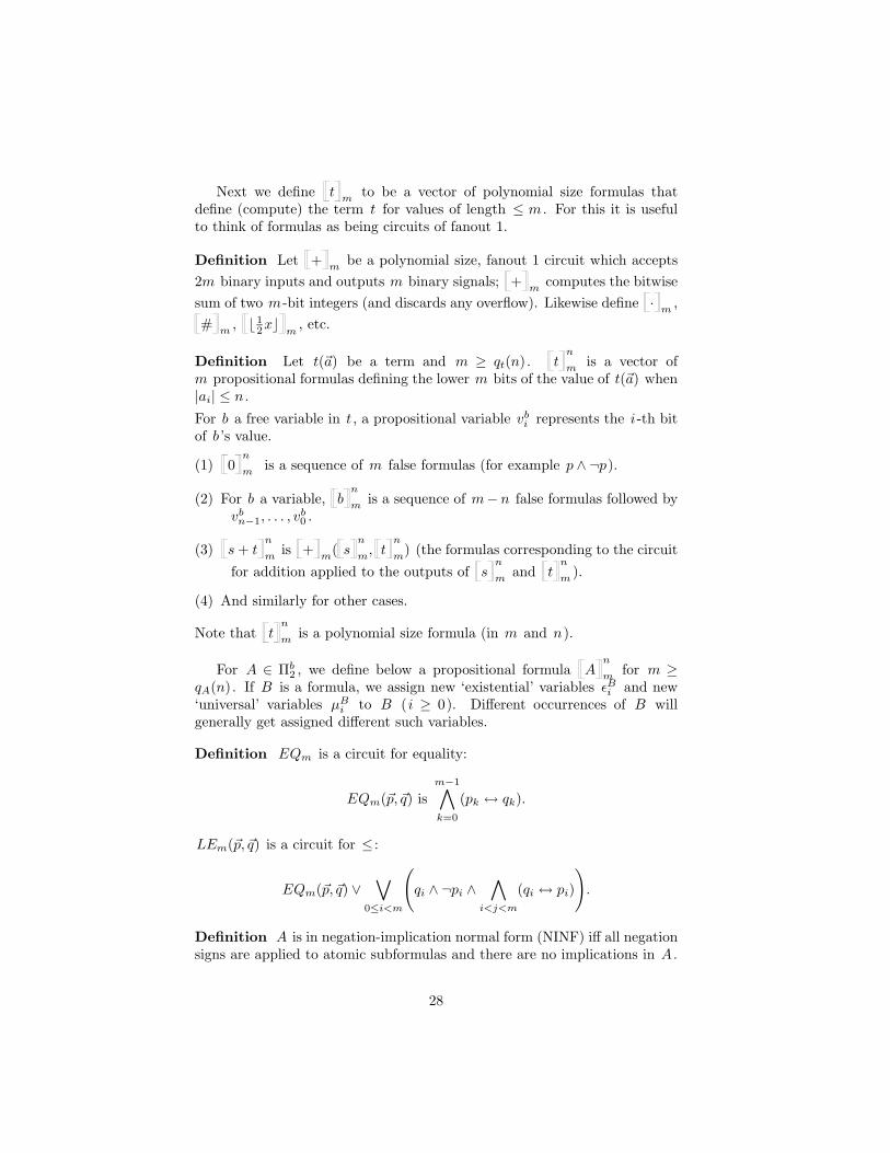
Next we define t m to be a vector of polynomial size formulas thatdefine (compute) the term t for values of length ≤ m . For this it is usefulto think of formulas as being circuits of fanout 1.

Definition Let +m

be a polynomial size, fanout 1 circuit which accepts2m binary inputs and outputs m binary signals; + m computes the bitwisesum of two m -bit integers (and discards any overflow). Likewise define · m ,# m , b 1

2xcm

, etc.

Definition Let t(~a) be a term and m ≥ qt(n). tn

mis a vector of

m propositional formulas defining the lower m bits of the value of t(~a) when|ai| ≤ n .

For b a free variable in t , a propositional variable vbi represents the i-th bit

of b ’s value.

(1) 0n

m is a sequence of m false formulas (for example p ∧ ¬p).

(2) For b a variable, bn

mis a sequence of m− n false formulas followed by

vbn−1, . . . , v

b0 .

(3) s + tn

m is + m( sn

m, tn

m) (the formulas corresponding to the circuit

for addition applied to the outputs of sn

m and tn

m ).

(4) And similarly for other cases.

Note that tn

m is a polynomial size formula (in m and n).

For A ∈ Πb2 , we define below a propositional formula A

n

mfor m ≥

qA(n). If B is a formula, we assign new ‘existential’ variables εBi and new

‘universal’ variables µBi to B (i ≥ 0). Different occurrences of B will

generally get assigned different such variables.

Definition EQm is a circuit for equality:

EQm(~p, ~q) ism−1∧k=0

(pk ↔ qk).

LEm(~p, ~q) is a circuit for ≤ :

EQm(~p, ~q) ∨∨

0≤i<m

(qi ∧ ¬pi ∧

∧i<j<m

(qi ↔ pi)

).

Definition A is in negation-implication normal form (NINF) iff all negationsigns are applied to atomic subformulas and there are no implications in A .

28

Definition Assume A ∈ Πb2 and A is in NINF and m ≥ qA(n). Define

An

minductively by:

(1) s = tn

m is EQm( sn

m, tn

m)

(2) s ≤ tn

mis LEm( s

n

m, t

n

m)

(3) ¬An

m is ¬ An

m for A atomic.

(4) A ∧ Bn

mis A

n

m∧ B

n

m

(5) A ∨ Bn

m is An

m ∨ Bn

m

(6) (∃x ≤ t)A(x)n

m is x ≤ t ∧ A(x)n

m(εAi /vx

i n−1i=0 )

(7) (∀x ≤ t)A(x)n

mis ¬x ≤ t ∨ A(x)

n

m(µA

i /vxi n−1

i=0 )

(8) (∀x ≤ |t|)A(x)n

mis

m−1∧k=0

¬k ≤ |t| ∨ A(k)n

mNote that |t| ≤ m (by our

assumption on m).

(9) (∃x ≤ |t|)A(x)n

m ism−1∨k=0

k ≤ |t| ∧ A(k)n

m

Proposition 29 The formula An

mis equivalent to A in that A(~a) is true

( |ai| ≤ n) iff for all truth assignments to the universal variables in An

m

there is an assignment to the existential variables which satisfies An

m .

We can extend the definition of A in the obvious way to formulas notin NINF, by using prenex operations to transform A into NINF form.

Definition An eF -proof of An

mis defined like an ordinary eF -proof

except now we additionally allow the existential variables (but not the othervariables) in A

n

mto be defined by the extension rule (each existential

variable may be defined only once).

Theorem 30 (essentially Cook [16]). If A ∈ Πb2 and S1

2 ` (∀~x)A(~x) thenthere are polynomial size (in n) eF -proofs of A

n

qA(n). These eF -proofs

are obtainable in polynomial time.

Proof If Γ→∆ is provable in S12 , we prove the theorem for

¬Γ ∨ ∆ .

By free-cut elimination it will suffice to do it for Γ ⊂ Σb1 and ∆ ⊂ Πb

2 . Weproceed by induction on the number of inferences in a free-cut free proof.

29

Case (1): A logical axiom B→B . Obviously

¬B ∨ B = ¬ B ∨ B

has a polynomial size eF -proof.Case (2): A BASIC axiom. For example,

(x + y) + z = x + (y + z)n

3n

has straightforward polynomial size F -proofs using techniques from [6] thatallow formalization of addition and multiplication in Frege proofs.

Case (3) The proof ends with a contraction:

Γ→∆, B,BΓ→∆, B

Recall that all three B ’s are assigned different existential and universalvariables. The induction hypothesis says there are polynomial size eF -proofsof

¬Γ ∨ ∆ ∨ B ∨ B .

Modify these proofs by (1) identifying the universal variables for differentB ’s; (2) at the end of the proof use extension to define

ε′′j ↔ ( B (~ε) ∧ εj) ∨ (¬ B (~ε) ∧ ε′j)

where ~ε′′ are the existential variables for the lower B and the others are theexistential variables for the upper B ’s; and (3) then extend to a proof of

¬Γ ∨ ∆ ∨ B (~ε′′).

Case (4) The proof ends with a Cut:

Γ→∆, B B,Π→ΛΓ,Π→∆,Λ

By free cut elimination, B ∈ Σb1 ; so B has existential variables ~ε and ¬B

has universal variables ~µ . By induction hypothesis, there are polynomialsize eF -proofs of

¬Γ ∨ ∆ ∨ B (~ε)

and¬Π ∨ Λ ∨ ¬B (~µ).

The polynomial size eF -proof of

¬Γ ∨ ¬Π ∨ ∆ ∨ Λ

30

consists of the first proof above followed by the second proof except with the~µ ’s changed to ~ε ’s followed by a (simulated) cut.

Case (5) For Σb1 -PIND inferences, iterate the construction for Cut and

contractions.

Case (6) If the proof ends with:

Γ→∆, A(t)t ≤ s,Γ→∆, (∃x ≤ s)A(x)

Let ~ε be the existential variables for (∃x ≤ s)A . The desired eF -proofcontains:

(a) Extension: ~ε ↔ t .(b) The proof from the induction hypothesis of

¬Γ ∨ ∆ ∨ A(t) .

(c) A further derivation of

¬t ≤ s ∨ ¬Γ ∨ ∆ ∨ (t ≤ s ∧ A(t)) .

(d) A derivation of

¬t ≤ s ∨ ¬Γ ∨ ∆ ∨ (∃x ≤ s)A(x)

by changing some t ’s to ε ’s. 2

6.2 Consequences of the S12 and eF Correspondence

Theorems 31-33 are due to Cook [16], although he stated them for PVinstead of for S1

2 .

Theorem 31 Let G ⊇ F be a propositional proof system. If S12 ` Con(G)

then eF p-simulates G .

Theorem 32 If S12 `NP=coNP then eF is super.

Theorem 33 eF has polynomial size proofs of the propositional formulasConeF (n) which assert that there is no eF -proof of p ∧ ¬p of length ≤ n .

Theorem 34 [9]. F has polynomial size proofs of the self-consistencyformulas ConF (n) .

31

Proof of Theorem 31 from Theorem 33: (Idea) Suppose there is a G proofP of a tautology ϕ . A polynomial size eF proof of ϕ is constructed asfollows: Let ~p be the free variables in ϕ(~p). Reason inside eF . First showthat if ¬ϕ then there is an F -proof P1 of ¬ϕ(~p) where ~p denotes a vectorof > ’s and ⊥ ’s: the truth values of ~p . By substituting ~p for ~p in P andcombining this with P1 , we construct a G -proof P2 of a contradiction. Thisproof has size polynomial in |P | since P1 has size polynomial in |ϕ| ≤ |P | .

By Theorem 33 there is a polynomial size eF -proof of ConG(|P2|) so theassumption that ¬ϕ is impossible; i.e., ϕ is true. 2

Proof of Theorem 33: S12 ` Con(eF). 2

Proof of Theorem 34: The F -self-consistency proof is a “brute-force” proofthat truth is preserved by axioms and modus ponens using the fact that theBoolean formula value problem is in ALOGTIME. 2

Definition A substitution Frege sF proof system is a Frege proof systemplus the substitution rule:

ψ(p)ψ(ϕ)

for ψ , ϕ arbitrary formulas, all occurrences of p substituted for.

Theorem 35 (Cook-Reckhow [19], Dowd [22], Krajıcek and Pudlak [33])sF and eF p-simulate each other.

Proof (Idea) sF p-simulates eF is not hard to show directly. eF p-simulates sF since S1

2 ` Con(sF). 2

6.3 Constant Depth Frege Proofs

Let propositional formulas use connectives ∧ and ∨ with negations onlyon variables. The depth of a formula is the maximum number of blocks(alternations) of ∧ ’s and ∨ ’s on any branch of the formula, viewed as a tree.The depth of a Frege proof is the maximum depth of formulas occurring inthe proof.

Theorem 36 Constant-depth Frege systems are complete (for constant depthtautologies).

Proof By the cut-elimination theorem. 2

32

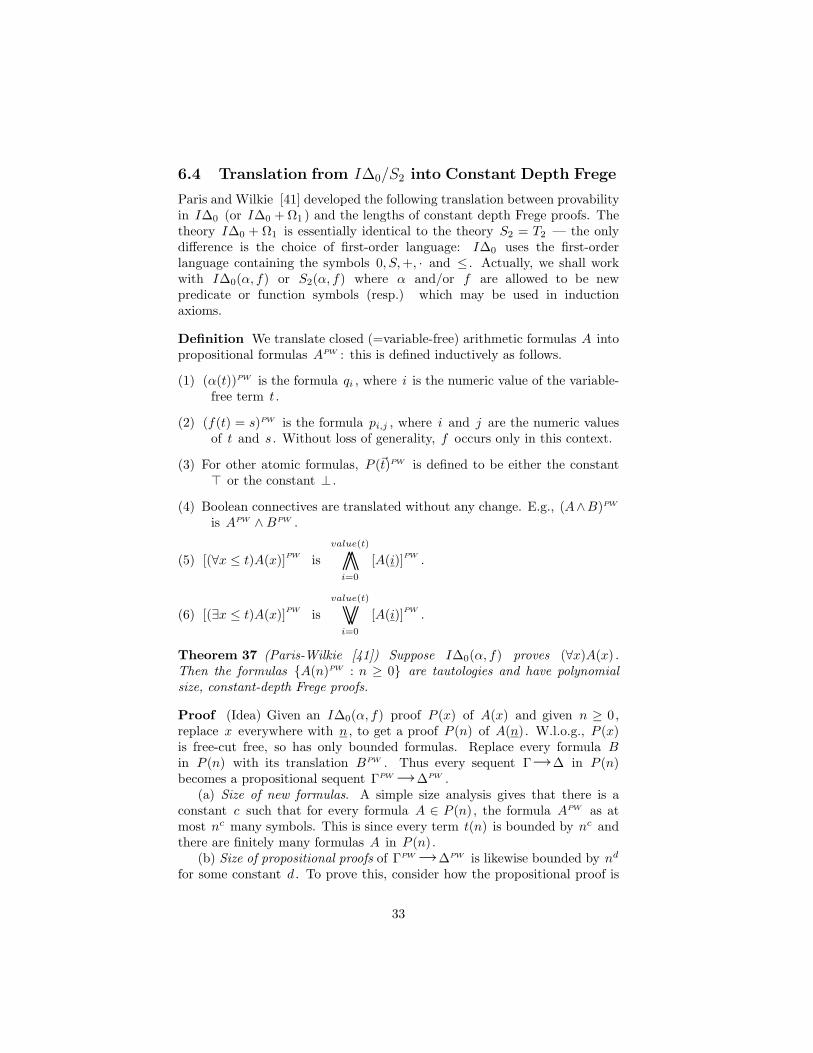
6.4 Translation from I∆0/S2 into Constant Depth Frege

Paris and Wilkie [41] developed the following translation between provabilityin I∆0 (or I∆0 + Ω1 ) and the lengths of constant depth Frege proofs. Thetheory I∆0 + Ω1 is essentially identical to the theory S2 = T2 — the onlydifference is the choice of first-order language: I∆0 uses the first-orderlanguage containing the symbols 0, S,+, · and ≤ . Actually, we shall workwith I∆0(α, f) or S2(α, f) where α and/or f are allowed to be newpredicate or function symbols (resp.) which may be used in inductionaxioms.

Definition We translate closed (=variable-free) arithmetic formulas A intopropositional formulas APW : this is defined inductively as follows.

(1) (α(t))PW is the formula qi , where i is the numeric value of the variable-free term t .

(2) (f(t) = s)PW is the formula pi,j , where i and j are the numeric valuesof t and s . Without loss of generality, f occurs only in this context.

(3) For other atomic formulas, P (~t)PW is defined to be either the constant> or the constant ⊥ .

(4) Boolean connectives are translated without any change. E.g., (A∧B)PW

is APW ∧ BPW .

(5) [(∀x ≤ t)A(x)]PW isvalue(t)∧∧

i=0

[A(i)]PW .

(6) [(∃x ≤ t)A(x)]PW isvalue(t)∨∨

i=0

[A(i)]PW .

Theorem 37 (Paris-Wilkie [41]) Suppose I∆0(α, f) proves (∀x)A(x) .Then the formulas A(n)PW : n ≥ 0 are tautologies and have polynomialsize, constant-depth Frege proofs.

Proof (Idea) Given an I∆0(α, f) proof P (x) of A(x) and given n ≥ 0,replace x everywhere with n , to get a proof P (n) of A(n). W.l.o.g., P (x)is free-cut free, so has only bounded formulas. Replace every formula Bin P (n) with its translation BPW . Thus every sequent Γ→∆ in P (n)becomes a propositional sequent ΓPW →∆PW .

(a) Size of new formulas. A simple size analysis gives that there is aconstant c such that for every formula A ∈ P (n), the formula APW as atmost nc many symbols. This is since every term t(n) is bounded by nc andthere are finitely many formulas A in P (n).

(b) Size of propositional proofs of ΓPW →∆PW is likewise bounded by nd

for some constant d . To prove this, consider how the propositional proof is

33

obtained from the proof P (n): the general idea is to work from the bottom ofthe proof upwards, always considering sequents in P (n) with values assignedto all the free variables.

(b.i) A ∃ ≤ :right inference in P (n):

Γ→ ∆, B(s)s ≤ t,Γ→ ∆, (∃x ≤ t)B(x)

If s ≤ t , the propositional translation of this is:

ΓPW → ∆PW , B(s)PW

∨ :right’s

ΓPW → ∆PW ,t∨∨

i=0

B(i)PW

>,ΓPW → ∆PW ,t∨∨

i=0

B(i)PW

(b.ii) A ∀ ≤ :right inference in P (n):

a ≤ t,Γ→ ∆, B(a)Γ→ ∆, (∀x ≤ t)B(x)

has propositional translation:

>,ΓPW → ∆PW , B(i)PWti=0 ∧ :right’s

ΓPW → ∆PW ,t∧∧

i=0

B(i)PW

(b.iii) A induction inference in P (n):

Γ, B(a)→ B(a + 1),∆Γ, B(0)→ B(t),∆

has propositional translation

ΓPW , B(i)PW → B(i + 1)PW ,∆PWt−1i=0

CutsΓPW , B(0)PW → B(t)PW ,∆PW

Other inferences are handled similarly. Since the proof P (n) has constantsize, and since the values of terms are ≤ nα , for some constant α , the sizebound is proved. 2

34

When Ω1 is present as an axiom, then the function x 7→ xlog x is total. Inthis case, an argument similar to the above establishes the following theorem:

Theorem 38 (Paris-Wilkie [41]) Suppose I∆0(α, f)+Ω1 proves (∀x)A(x) .Then the formulas A(n)PW : n ≥ 0 are tautologies and have quasi-polynomial size, constant-depth Frege proofs.

The above two theorems can be sharpened in the case of Si2 - and

T i2 -proofs. First, at the cost of adding a finite set polynomial time functions

such as the Godel β function, we may assume that every formula in Σbi (α, f)

or Πbi (α, f) consists of exactly i bounded quantifiers, then a sharply bounded

quantifier and then a Boolean combination of atomic formulas of the formα(t) or f(t) = s or which do not use α or f . [Basically, because of thequantifier exchange property and by contracting like quantifiers.] With thisconvention, then if A ∈ Σb

i or A ∈ Πbi then the translation APW is a depth

i + 1 propositional formula where the bottom depth has polylogarithmicfanin. This gives the following theorem:

Theorem 39 Suppose T i2 ` Γ→∆ , sequent of Σb

i ∪ Πbi formulas. Then

the sequents ΓPW →∆PW have polynomial size propositional sequent calculusproofs of depth i + 1 in which every formula has polylogarithmic fanin at thebottom level.

Furthermore, there is a constant c such that every sequent in thepropositional proof has at most c formulas.

If every formula in the T i2 -proof is in Πb

i , then every formula in thepropositional proofs starts with a (topmost) block of

∧’s.

Proof Analogous to the above proof. We leave the details to the reader.

7 Interpolation Theorems for PropositionalLogic

7.1 Craig’s Theorem

The interpolation theorem is one of the fundamental theorems of mathemat-ical logic; this was first proved in the setting of first-order logic by Craig [20].For propositional logic, the interpolation is much simpler:

Theorem 40 Let A(~p, ~q) and B(~p, ~r) be propositional formulas involvingonly the indicated variables. Suppose A(~p, ~q) ⊃ B(~p, ~r) is a tautology. Thenthere is a propositional formula C(~p) using only the common variables, sothat A ⊃ C and C ⊃ B are tautologies.

Proof Since A(~p, ~q) |= B(~p, ~r); if we have already assigned truth values to~p = p1, . . . , pk , then it is not possible to extend this to a truth assignmenton ~p, ~q, ~r such that both A(~p, ~q) and ¬B(~p, ~r) hold.

35

Let τ1, . . . , τn be the truth assignments to p1, . . . , pk for which it ispossible to make A(~p, ~q) true by further assignment of truth values to ~q .

Let C(~p) say that one of τ1, . . . , τn holds for ~p , i.e.,

C =n∨∨

i=1

(p(i)1 ∧ p

(i)2 ∧ . . . ∧ p

(i)k

)where

p(i)j =

pj if τi(pj) =True¬pj otherwise

Then clearly, A(~p, ~q) |= C(~p). Also, by the comment at the beginning of theproof, C(~p) |= B(~p, ~r). 2

Note that C(~p) may be exponentially larger than A(~p, ~q) and B(~p, ~r).

Example: Let p1, . . . , pk code the binary representation of a k -bitinteger P . Let A(~p, ~q) be a formula which is satisfiable iff P is composite(e.g. q codes two integers > 1 with product P ). Let B(~p, ~r) be a formulawhich is satisfiable iff P is prime (i.e., ~r codes a Pratt-primality witness).

P is prime ⇔ ∃~rB(~p, ~r)⇔ ¬∃~qA(~p, ~q).

and A(~p, ~q) ⊃ ¬B(~p, ~r) is a tautology.An interpolant C(~p) must express “~p codes a composite”.

Generalizing the above example gives:

Theorem 41 (Mundici [37] If there is a polynomial upper bound on thecircuit size of interpolants in propositional logic, then

NP/poly ∩ coNP/poly = P/poly

Proof Let ∃~qA(~p, ~q) express an NP/poly property R(~p) and ∀~rB(~p, ~r)express R(~p) in coNP/poly form. Then

∃~qA(~p, ~q) |= ∀~rB(~p, ~r),

which is equivalent toA(~p, ~q) ⊃ B(~p, ~r)

being a tautology. Let C(~p) be a polynomial size interpolant s.t.,

A(~p, ~q) ⊃ C(~p) and C(~p) ⊃ B(~p, ~r)

are tautologies. Thus

∃~qA(~p, ~q) |= C(~p) |= ∀~rB(~p, ~r),

I.e., R(~p) ⇔ C(~p) and R(~p) has a polynomial size circuit, so R(~p) is inP/poly . 2

36

7.2 Cut-Free Proofs and Interpolant Size

Definition Let PK be the propositional fragment of the Gentzen sequentcalculus. The size of a PK -proof, |P | , is the number of steps in P .Normally, sequent calculus proofs are treelike; however, sometime we considernon-treelike proofs, and in this case, we write |P |dag to denote the size of P .V (A) denotes the set of free variables in A . For C a formula, |C| is thenumber of ∧ ’s and ∨ ’s in C .

The next theorem states that tree-like cut-free proofs have interpolantsof polynomial formula size, and general cut-free proofs have interpolants ofpolynomial circuit size.

Theorem 42 Let P be a cut-free PK proof of A→B , where V (A) ⊆ ~p, ~qand V (B) ⊆ ~p, ~q . Then there is an interpolant C such that

(1) A ⊃ C and C ⊃ B are valid,

(2) V (C) ⊆ ~p ,

(3) |C| ≤ |P | and |C|dag ≤ |P |dag .

Remark: The theorem also holds for proofs which have cuts only onformulas D such that V (D) ⊆ ~p, ~r or V (D) ⊆ ~p, ~r .

Proof We use induction on the number of inferences in P to prove a slightlymore general statement:

Claim: If P is a proof of Γ1,Γ2→∆1,∆2 and if V (Γ1,∆1) ⊆ ~p, ~q andV (Γ2,∆2) ⊆ ~p, ~r , then there is an interpolant C so that

(1) Γ1→∆1, C and C,Γ2→∆2 are valid,

(2) V (C) ⊆ ~p , and

(3) The polynomial size bounds hold too.

Base Case: Initial sequent. If the initial sequent is of the form qi→qi , takeC to be ⊥ since

qi→qi,⊥ and ⊥→are valid. For an initial sequent of the form ri→ri , take C to be > . Foran initial sequent pi→pi , C will be either > , ⊥ , pi or (¬pi) dependingon how the pi ’s are split into Γ1,Γ2,∆1,∆2 .

Induction Step: There are a number of cases, depending on the type of thelast inference in the proof.

(1) For last inference an ∨ :right:

37

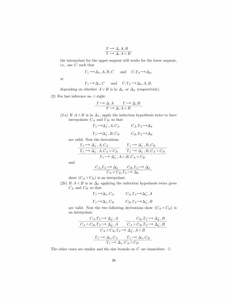
Γ→ ∆, A,B

Γ→ ∆, A ∨ B

the interpolant for the upper sequent still works for the lower sequent,i.e., use C such that

Γ1→∆1, A,B,C and C,Γ2→∆2,

orΓ1→∆1, C and C,Γ2→∆2, A,B,

depending on whether A ∨ B is in ∆1 or ∆2 (respectively).

(2) For last inference an ∧ :right:

Γ→ ∆, A Γ→ ∆, B

Γ→ ∆, A ∧ B

(2.a) If A ∧ B is in ∆1 , apply the induction hypothesis twice to haveinterpolants CA and CB so that

Γ1→∆−1 , A,CA CA,Γ2→∆2

Γ1→∆−1 , B,CB CB ,Γ2→∆2

are valid. Now the derivationsΓ1→ ∆−

1 , A,CA

Γ1→ ∆−1 , A,CA ∨ CB

Γ1→ ∆−1 , B,CB

Γ1→ ∆−1 , B,CA ∨ CB

Γ1→ ∆−1 , A ∧ B,CA ∨ CB

andCA,Γ2→ ∆2 CB ,Γ2→ ∆2

CA ∨ CB ,Γ2→ ∆2

show (CA ∨ CB) is an interpolant.(2b) If A ∧ B is in ∆2 applying the induction hypothesis twice gives

CA and CB so that

Γ1→∆1, CA CA,Γ2→∆−2 , A

Γ1→∆1, CB CB ,Γ2→∆−2 , B

are valid. Now the two following derivations show (CA ∧ CB) isan interpolant:

CA,Γ2→ ∆−2 , A

CA ∧ CB ,Γ2→ ∆−2 , A

CB ,Γ2→ ∆−2 , B

CA ∧ CB ,Γ2→ ∆−2 , B

CA ∧ CB ,Γ2→ ∆−2 , A ∧ B

Γ1→ ∆1, CA Γ1→ ∆1, CB

Γ1→ ∆1, CA ∧ CB

The other cases are similar and the size bounds on C are immediate. 2

38

7.3 Interpolation Theorems for Resolution

We start with a quick review of the well-known system of resolution forpropositional logic.

Definition A literal is a propositional variable p or a negated variable ¬p .p is ¬p , and (¬p) is p . A clause is a set of literals; its intended meaning isthe disjunction of its members. A set of clauses represents the conjunctionof its members. Thus a set of clauses “is” a formula in conjunctive normalform. A resolution inference is an inference of the form:

C ∪ p D ∪ pC ∪ D

For such resolution inferences, we assume w.l.o.g. that p, p 6∈ C and p, p 6∈ D .A resolution refutation of a set Γ of clauses is a derivation of the emptyclause ∅ from Γ by resolution inferences.

Theorem 43 Resolution is refutation-complete (and sound).

Since resolution is a refutation, it does not prove implications A ⊃ B .Therefore, to formulate the interpolation theorem for resolution, we workwith sets of clauses A ∪ B . An interpolant for the sets A and B is aformula C such that A ⊃ C and C ⊃ ¬B . This gives the following form ofthe interpolation theorem:

Theorem 44 Let A1(~p, ~q), . . . , Ak(~p, ~q) and B1(~p, ~r), . . . , B`(~p, ~r) besets of clauses, so that their union Γ is inconsistent. Then there is aformula C(~p) such that for any truth assignment τ , domain(τ) ⊇ ~p, ~q, ~r ,

(1) If τ(C(~p)) = False, then τ(Ai(~p, ~q)) = False, for some i .

(2) If τ(C(~p)) = True, then τ(Bj(~p, ~q)) = False, for some j .

Proof From Γ unsatisfiable, we have

A1(~p, ~q), . . . , Ak(~p, ~q)→¬B1(~p, ~r), . . . ,¬B`(~p, ~r)

is valid. Thus there is an interpolant C(~p) such that

A1(~p, ~q), . . . , Ak(~p, ~q)→C(~p)

andC(~p)→¬B1(~p, ~r), . . . ,¬B`(~p, ~r)

are valid. 2

The next theorem gives bounds on the size or computational complexityof the interpolant, in terms of the number of inferences in the resolutionrefutation.

39

Theorem 45 (Krajıcek [32]) Let Ai(~p, ~q)i ∪ Bj(~p, ~r)j have a refutationR of n resolution inferences. Then an interpolant, C(~p) , can be chosen withO(n) symbols in dag representation.

If R is tree-like, then C(~p) is a formula with O(n) symbols.

Proof We view R as a dag or as a tree, each node corresponding to aninference and labeled with the clause inferred at that inference. For eachclause E in R , define CE(~p) as follows:

(1) For E = Ai(~p, ~q), a hypothesis, set CE = ⊥ (False).

(2) For E = Bj(~p, ~q), a hypothesis, set CE = > (True).

(3) For an inferenceF ∪ qi G ∪ qi

F ∪ G

set CF∪G = CF∪qi ∨ CG∪qi .

(4) For an inferenceF ∪ ri G ∪ ri

F ∪ G

set CF∪G = CF∪ri ∧ CG∪ri .

(5) For an inferenceF ∪ pi G ∪ pi

F ∪ G

set CF∪G = (pi ∧ CF∪pi) ∨ (pi ∧ CG∪pi).

Lemma 46 For all clauses F ∈ R , CF (~p) satisfies the following conditionthat if τ is a truth assignment and τ(F ) = False, then

(a) if τ(CF ) = False, then τ(Ai(~p, ~q)) = False for some i

(b) if τ(CF ) = True, then τ(Bj(~p, ~r)) = False for some j

The proof of the lemma is by induction on the definition of CF .Q.E.D. Lemma and Theorem.

7.4 Resolution with Limited Extension

By “extension” is meant the introduction of variables that represent complexpropositional formulas. We have already seen one system that uses extension,namely the extended Frege proof system. “Limited extension” means thatextension variables may be introduced to abbreviate only formulas thatappear in the formula being proved.

When A is a formula, we let σA be the extension variable for A ; inparticular, for p a variable, σp is just the same variable p , and for otherformulas A , σA is a new variable.

40

Definition When A is a formula, LE(A) is a set of clauses which definethe meanings of the extensions variables for all subformulas of A; to wit:

LE(p) = ∅

LE(¬A) = LE(A) ∪σ¬A, σA︸ ︷︷ ︸¬σA⊃σ¬A

, σ¬A, σA︸ ︷︷ ︸σ¬A⊃¬σA

LE(A∧B) = LE(A)∪LE(B)∪σA∧B, σA︸ ︷︷ ︸

σA∧B⊃σA

, σA∧B, σB︸ ︷︷ ︸σA∧B⊃σB

, σA∧B, σA, σB︸ ︷︷ ︸σA∧σB⊃σA∧B

LE(A∨B) = LE(A)∪LE(B)∪σA, σA∨B︸ ︷︷ ︸

σA⊃σA∨B

, σB, σA∨B︸ ︷︷ ︸σB⊃σA∨B

, σA, σB, σA∨B︸ ︷︷ ︸σA∨B⊃σA∨σB

Definition Let A be a set of formulas. Then LE(A) is ∪A∈ALE(A) .Similarly,

LE(~p, ~q) = ∪LE(A) : V (A) ⊆ ~p, ~q.LE(~p, ~r) = ∪LE(A) : V (A) ⊆ ~p, ~r.

Theorem 47 Let Γ be the set of clauses

Ai(~p, ~q)i ∪ Bj(~p, ~r)j ∪ LE(~p, ~q) ∪ LE(~p, ~r)

and suppose Γ has a refutation R of n resolution inferences. Then there isan interpolant C(~p) for the sets Ai(~p, ~q)i and Bj(~p, ~r)j of circuit sizeO(n) .

Proof Let C(~p) be the interpolant for Ai(~p, ~q)i ∪ LE(~p, ~q) andBj(~p, ~r)j ∪ LE(~p, ~r) given by the earlier interpolation theorem.

Claim C(~p) is the desired interpolant.

Proof of claim: Any truth assignment τ with domain ~p, ~q can beuniquely extended to satisfy LE(~p, ~q). Suppose τ(C(~p)) = False . Extendτ so as to satisfy LE(~p, ~q). By choice of C(~p), τ makes a clause fromAi(~p, ~q)i ∪ LE(~p, ~q) false, hence makes one of the Ai ’s false.

A similar argument shows that if τ(C(~p)) = True , then τ falsifies someBj(~p, ~r).Q.E.D. Claim and Theorem.

41

8 Natural Proofs, Interpolation and BoundedArithmetic

8.1 Natural Proofs

The notion of natural proofs was introduced by Razborov and Rudich [44].In order for a proof to be a natural proof of P 6= NP, it must give asuitably constructive way of proving that certain Boolean functions are notin P (for example, the Boolean function Sat which recognized satisfiablepropositional formulas). More precisely, a proof is natural provided it ispossible to use the proof method to find a family Cn of Boolean functionswhich satisfies the property of the next definition. We represent a Booleanfunction fn(x1, . . . , xn) by its truth table (which of course has size N = 2n );therefore, an n -ary Boolean functions is identified with a string of 2n 0’sand 1’s.

Definition C = Cnn is quasipolynomial-time natural against P/poly ifand only if each Cn is a set of (strings representing) truth tables of n -aryBoolean functions, and such that the following hold:

Constructivity: The predicate “fn ∈ Cn ?” has circuits of size 2nO(1), and

Largeness: |Cn| ≥ 2−cn · 22n

for some c > 0, and

Usefulness: If fn ∈ Cn for all n , then the family fnn is not in P/poly(i.e., does not have polynomial size circuits).

The motivation for this definition of natural proofs is that “constructive”proofs that NP 6⊂ P/poly ought to give (quasi)polynomial time propertywhich is natural against P/poly . Note that ‘quasipolynomial time’, ismeasured as a function of the size of the truth table of fn .

8.2 Strong Pseudo-Random Number Generator Conjec-ture

We now introduce the Strong Pseudo-Random Number Generator (SPRNG)Conjecture: this conjecture implies the existence of pseudorandom numbergenerators which generate pseudorandom numbers that pass any feasibletest for randomness. This conjecture is closely related to the problem of theexistence of one-way functions, and is generally conjectured to be true byresearchers in cryptography. (But it is stronger that P 6= NP, and so far ithas not been proven.)

Definition Let Gn : 0, 1n → 0, 12n be a pseudo-random numbergenerator. The hardness, H(Gn), of Gn is the least S > 0 such that, for

42

some circuit C of size S ,∣∣∣∣ Probx∈0,1n

[C(Gn(x))=1] − Proby∈0,12n

[C(y)=1]∣∣∣∣ ≥ 1

S

SPRNG Conjecture: There are pseudorandom number generators Gn ,computed by polynomial size circuits, with hardness H(Gn) ≥ 2nε

, for someε > 0.

One of the main results of Razborov and Rudich [44] is the followingtheorem. We omit the proof from these notes.

Theorem 48 If the SPRNG conjecture is true, then there are no propertieswhich are quasipolynomial time/poly natural against P/poly .

The remainder of this article presents a theorem of Razborov that states,in essence, that if S2

2 can prove certain kinds of superpolynomial lowerbounds on the sizes of circuits for polynomial hierarchy predicates (e.g., thatSAT is not in NP), then there is a natural proof that P 6= NP which,by the previous theorem, would imply the falsity of the SPRNG conjecture.Since the SPRNG conjecture is thought to be true, then we do not expectto be able to obtain such a lower bound proof in S2

2 .Let α be a new predicate symbol: we will use α to encode information

about a Boolean circuit. Let LB(t, S, α) be a formula which states thatthe Boolean circuit encoded by α either does not correctly compute thepredicate S or has size greater than t . In other words, proving LB(t, S, α)proves that t is a lower bound on the size of any circuit computing S . (Wegive a more complete definition of LB() in the next section.)

Razborov [43] proved the following theorem:

Theorem 49 Let t denote any superpolynomial function and let S be anybounded formula. If S2

2(α) proves LB(t, S, α) , then the SPRNG conjectureis false.

Razborov’s first proof of Theorem 49 used the conservativity of S22(α)

over T 12 (α) and used the resulting PLS algorithm to construct a kind of

interpolant which serves as a natural proof. He later gave a second, moredirect proof based on translating T 1

2 (α)-proofs into propositional proofs [42].We give below a variation of this second proof based on propositionalinterpolation theorems, using a translation of T 1

2 (α) proofs into limitedextension resolution refutations, generalizing a construction of Krajıcek [32].

The remainder of this article is devoted to this proof.

8.3 Split Bounded Arithmetic Theories

Let α and β be new unary predicate symbols. We define theories Si2(α, β)

and T i2(α, β) of bounded arithmetic in the usual way by adjoining α and β

as new predicate symbols. In addition, these theories admit induction on

43

Σbi (α, β)-formulas (which are Σb

i -formulas in which α and β may appear).We let Σb

∞(α) denote all bounded formulas in the language of S2 plus α .And we define the class of formulas SΣb

i to equal

SΣbi = Σb

i (Σb∞(α),Σb

∞(β))

where Σb1(X) indicates the closure of X under ∧ , ∨ , sharply bounded

quantification and existential bounded quantification, where Πb1(X) is

defined similarly andΣb

i+1(X) = Σb1(Π

bi (X))

and Πbi+1(X) is similarly defined.

The split versions of Si2 and T i

2 are defined as follows:

Definition

SSi2 = BASIC + SΣb

i -PINDST i

2 = BASIC + SΣbi -IND

We now describe the way in which circuits are coded in the theories Si2(α)

and T i2(α), and the way in which superpolynomial lower bounds on circuit

size are expressed in these theories. Let N ≥ 0 and n = |N | ≈ log N ( wheren = |x|). Also suppose t(n) = nω(1) (this will be the superpolynomial lowerbound) — note that the fact that t(n) = nω(1) need not be provable in S2 .Finally, suppose that S(N,x) is a Σb

∞ -formula.

Definition Let LB(t, S, α) be the statement

¬[α codes a circuit of size ≤ t(n) such that

(∀x ∈ 0, 1n)(α(x) = 1 ↔ S(N,x))]

where

(1) The free variables of LB(t, S, α) are N and α .

(2) By “α encodes a circuit” we mean that α encodes gate types and gateconnections in some straightforward manner, plus, α may encode thefull truth table description of the functions computed by every gate inthe circuit!

Theorem 50 If S22(α) ` LB(t, S, α) , then SS2

2 ` SLB(t, S, α, β) whereSLB(t, S, α, β) is

¬[α codes a circuit of size ≤ t(n)/2 − 1 and

β codes a circuit of size ≤ t(n)/2 − 1 such that

∀x ∈ 0, 1n((α ⊕ β)(x) = 1 ↔ S(N,x))]

44

Proof If ¬SLB(t, S, α, β), then the circuit α′

¯¯¯¯¯

LL

LL

LL

¯¯¯¯¯

LL

LL

LL

⊕¡

¡¡

@@@

α β

α′

satisfies ¬LB(t, S, α). 2

In order to rephrase SLB(t, S, α, β), we let γ be a new predicate symbol.Theories such as SS(α, β)22 and ST 1

2 (α, β) may use the symbol γ in inductionformulas. If

SS22 ` SLB(t, S, α, β),

thenSS2

2 ` ¬CC(t/2 − 1, γ, α) ∨ ¬CC(t/2 − 1, S ⊕ γ, β)

where CC(t, T (x), α) states:[α codes a circuit of size ≤ t(n) such that

∀x ∈ 0, 1n(α(x) = 1 ↔ T (x))]

or, in sequent form, SS22 proves

CC(t/2 − 1, γ, α), CC(t/2 − 1, S ⊕ γ, β)→Since CC is a Σb

1 formula, this sequent is also provable in ST 12 by ∀Σb

2 -conservativity. (By the same proof that shows S2

2 is conservative overT 1

2 .)

Theorem 51 (Razborov [43]) If SS22 ` SLB(t, S, α, β) for some t = nω(1)

and S ∈ Σb∞ , then the SPRNG conjecture is false.

Corollary 52 If the SPRNG conjecture holds, then S22 does not prove

superpolynomial lower bounds on circuit size for any bounded formula (i.e.,for any polynomial time hierarchy predicate).

The proof of Theorem 51 takes up the rest of this paper. We shall provethat if

ST 12 ` CC(t, γ, α), CC(t, S ⊕ γ, β)→ ,

45

then there are quasipolynomial size circuits which are natural against P/poly .The first step of the proof involves converting an ST 1

2 -proof and thesequent into a constant-depth propositional proof using the general methodof Theorem 38. We then convert this to a resolution refutation with limitedextension and finally apply the Interpolation Theorem 47. The interpolantobtained in this way will serve as a natural proof against P/poly .

8.4 Conversion to Constant Depth Frege Proofs

In this section, we discuss how to apply the Paris-Wilkie translation ofTheorem 38 to T 1

2 (α, β) proofs. The proof of Theorem 38 still mostlyapplies, and the only new ingredient required for the translation is thatwe must describe the translation of atomic formulas β(t) and γ(t). Thisis easily done by augmenting the definition of section 6.4 above to define(β(t))PW to equal ri and (γ(t))PW to equal pi , where i is the numeric valueof the closed term t .

By expanding the language to include the sequence coding functions andusing SΠb

1 -IND and applying free cut-elimination, we may assume that everyformula in the ST 1

2 proof is of the form

(∀y ≤ r)(∃z ≤ |r′|)(· · ·)

where (· · ·) is a Boolean combination of Σb∞(α) formulas and Πb

∞(β)formulas and of formulas γ(· · ·).

When translated into propositional logic by the Paris-Wilkie translation,this becomes

2nO(1)∧∧i=0

nO(1)∨j=0

Ei,j

where each formula Ei,j either (1) is ±pi or (2) involves only ~p, ~q or(3) involves only ~p, ~r .

Suppose we have a ST 12 -proof of

CC(t, γ, α), CC(t, S ⊕ γ, β)→ ,

Fixing N and f(x) = S(N,α), the Paris-Wilkie translation gives apropositional sequent calculus proof of∧∧

i

Ai(~p, ~q),∧∧j

Bj(~p, ~r)→

where

(1) Ai(~p, ~q)i is a set of clauses stating that ~q codes a circuit of size tcomputing the function γ with graph given by ~p .

46

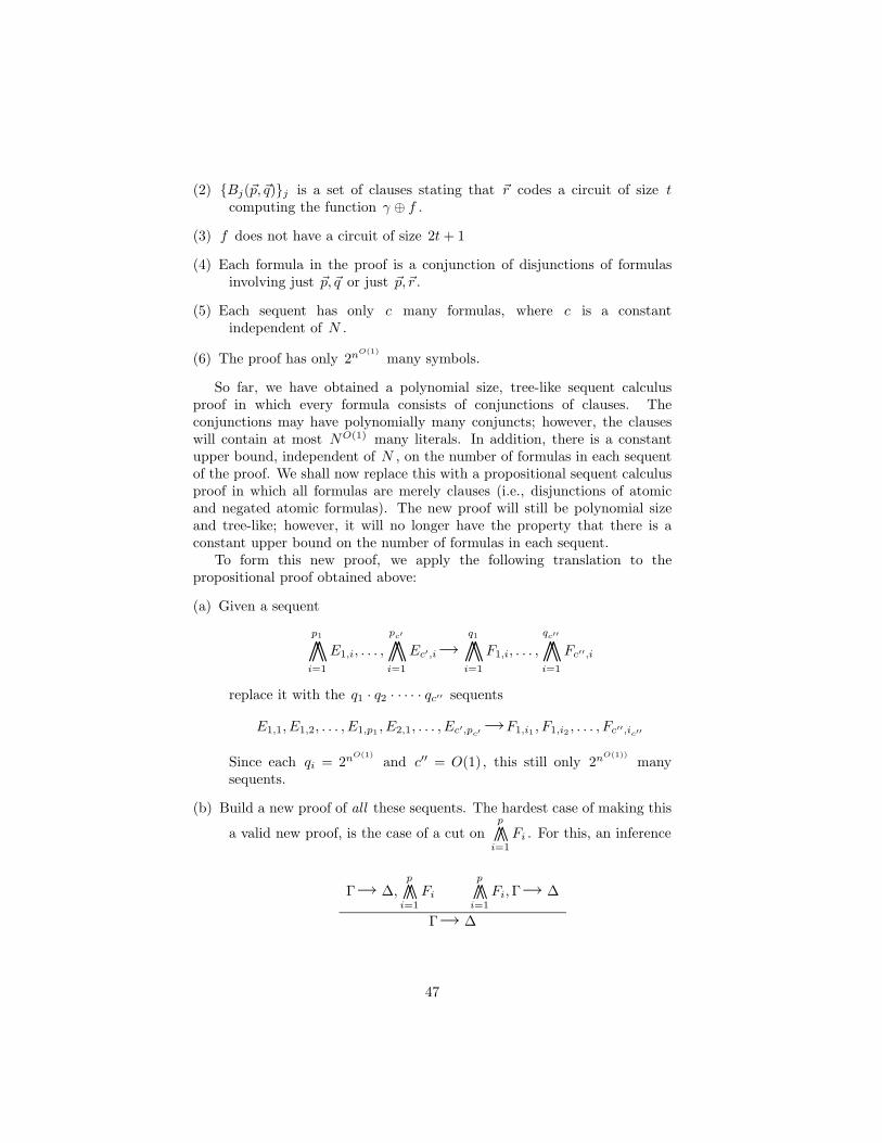
(2) Bj(~p, ~q)j is a set of clauses stating that ~r codes a circuit of size tcomputing the function γ ⊕ f .

(3) f does not have a circuit of size 2t + 1

(4) Each formula in the proof is a conjunction of disjunctions of formulasinvolving just ~p, ~q or just ~p, ~r .

(5) Each sequent has only c many formulas, where c is a constantindependent of N .

(6) The proof has only 2nO(1)many symbols.

So far, we have obtained a polynomial size, tree-like sequent calculusproof in which every formula consists of conjunctions of clauses. Theconjunctions may have polynomially many conjuncts; however, the clauseswill contain at most NO(1) many literals. In addition, there is a constantupper bound, independent of N , on the number of formulas in each sequentof the proof. We shall now replace this with a propositional sequent calculusproof in which all formulas are merely clauses (i.e., disjunctions of atomicand negated atomic formulas). The new proof will still be polynomial sizeand tree-like; however, it will no longer have the property that there is aconstant upper bound on the number of formulas in each sequent.

To form this new proof, we apply the following translation to thepropositional proof obtained above:

(a) Given a sequent

p1∧∧i=1

E1,i, . . . ,

pc′∧∧i=1

Ec′,i→q1∧∧

i=1

F1,i, . . . ,

qc′′∧∧i=1

Fc′′,i

replace it with the q1 · q2 · · · · · qc′′ sequents

E1,1, E1,2, . . . , E1,p1 , E2,1, . . . , Ec′,pc′ →F1,i1 , F1,i2 , . . . , Fc′′,ic′′

Since each qi = 2nO(1)and c′′ = O(1), this still only 2nO(1))

manysequents.

(b) Build a new proof of all these sequents. The hardest case of making this

a valid new proof, is the case of a cut onp∧∧

i=1

Fi . For this, an inference

Γ→ ∆,p∧∧

i=1

Fi

p∧∧i=1

Fi,Γ→ ∆

Γ→ ∆

47

is replaced by p cuts; i.e., by

Γ∗→ ∆∗, F3

Γ∗→ ∆∗, F2

Γ∗→ ∆∗, F1 F1, F2, . . . , Fp,Γ∗→ ∆∗

F2, F3, . . . , Fp,Γ∗→ ∆∗

F3, . . . , Fp,Γ∗→ ∆∗

···

Γ∗→ ∆∗

At the end of the second step, we have a treelike sequent calculus proof of

A1(~p, ~q), . . . , Ak(~p, ~q), B1(~p, ~r), . . . B`(~p, ~r)→such that every formula in in the proof is a disjunction of formulas whicheither involve just ~p and ~q or involve just ~p and ~r .

8.5 Translation to Resolution with Limited Extension

In the previous section, we have converted the ST 12 (α, β)-proof into a

polynomial size, tree-like, propositional sequent calculus proof containingonly clauses as formulas. We next shall convert this proof into a resolutionrefutation with limited extension.

Each sequent in the proof obtained in the second step has the formp1∨

i=1

E1,i, . . . ,

pu∨i=1

Eu,i, →q1∨

i=1

F1,i, . . . ,

qv∨i=1

Fv,i (A)

where each Ea,i , Fa,i involves only ~p, ~q or ~p, ~r .Associate with sequent (A), the following set (B) of clauses:

E1,ip1i=1, . . . , Eu,ipu

i=1, ¬F1,1, , ¬F1,2, , . . . , ¬Fv,qv, (B)

Now (B) is not really a proper set of clauses, since clauses are supposedto contain literals (not formulas). So instead of using (B), we introduceextension variables to form the following set (C) of clauses:σE1,i

p1i=1, . . . , σEu,i

pu

i=1, σ¬F1,1, σ¬F1,2, . . . , σ¬Fv,qv (C)

If sequent (A) is Γ→∆, then the set (C) of clauses is denoted (Γ→∆)LE .It is important for us that all the extension variables used in (C) are fromLE(~p, ~q) and LE(~p, ~r).

Lemma 53 If Γ→∆ is derived in m lines of the sequent calculus proofconstructed in Step (2) above, then

(Γ→∆)LE ∪ LE(~p, ~q) ∪ LE(~p, ~r)

has a resolution refutation (not necessarily tree-like) of O(m2) resolutioninferences.

48

Proof By induction on m . — splits into cases depending on the lastinference of the proof:

Case (1) Γ→∆ is A→A . If A =∨

Ai , then

σA1 , . . . , σAu, σ¬A1, . . . , σ¬Au

∪ LE(A)

has a resolution refutation of O(u) inferences.

Case (2) Suppose A =∨

i Ai involves only ~p, ~q . Then σA andσA1 , . . . , σAu

can be derived from each other (in the presence ofLE(A)). Therefore it is not important how we express formulas asdisjunctions when there is a choice.

Case (3) ∧ :left and ∨ :right inferences involve only formulas that use just~p, ~q or just ~p, ~r ; these are therefore straightforward (the ∧ :right is alittle harder than the ∨ :left case).

Case (4) An ∨ :left inference can be:

∨i Ei,Γ→ ∆

∨j Fj ,Γ→ ∆

∨Ei, Fji,j ,Γ→ ∆

The induction hypotheses give refutations R1 and R2 :

(Γ→∆)LE

σEii

LE(~p, ~q)LE(~p, ~r)

R1=⇒ ∅

and(Γ→∆)LE

σFjj

LE(~p, ~q)LE(~p, ~r)

R2=⇒ ∅

These can be combined as:

(Γ→∆)LE

σEii ∪ σFj

j

LE(~p, ~q)LE(~p, ~r)

R′1=⇒ σFj

j

(Γ→∆)LE

LE(~p, ~q)LE(~p, ~r)

R2=⇒ ∅

where R′1 is like R1 but uses σEi

i ∪ σFjj in place of σEi

i .

(Remark: Note the refutation is not tree-like since σFjj may be used

multiple times in R2 .)

49

Case 5 Suppose the last inference is a cut:

Γ→ ∆,∨

i Ai

∨i Ai,Γ→ ∆

Γ→ ∆

The induction hypotheses give refutations R1 and R2 :

(Γ→∆)LE

σ¬A1, . . . , σ¬Au

LE(~p, ~q)LE(~p, ~r)

R1=⇒ ∅

and

(Γ→∆)LE

σA1 , . . . , σAu

LE(~p, ~q)LE(~p, ~r)

R2=⇒ ∅

Combine these as below, with R′1 equal to R1 minus any uses of

σ¬Ai ’s:

(Γ→∆)LE

LE(~p, ~q)LE(~p, ~r)

R′

1=⇒ σA1 , . . . , σAu

(Γ→∆)LE

LE(~p, ~q)LE(~p, ~r)

R2=⇒ ∅

Q.E.D. Lemma.

8.6 Conclusion of the Proof

From the previous Lemma 53 and from the Interpolation Theorem 47 forresolution with limited extension, there must be a circuit C(~p) of size 2nO(1)

such that

(1) if C(~p) = 0, then Ai(~p, ~q)i is unsatisfiable, and

(2) if C(~p) = 1, then Bj(~p, ~q)j is unsatisfiable.

Note the size of C(~p) is 2nO(1)which is quasipolynomial in N = 2n . In

case (1), when C(~p) = 0, the function γ(x) does not have a circuit of sizet = nω(1) . In case (2), when C(~p) = 1, the function (γ ⊕ f)(x) does nothave a circuit of size t = nω(1) . (Recall f(x) does not have a circuit of size2t + 1.)

50

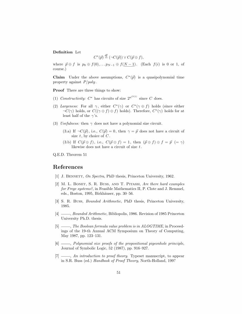
Definition LetC∗(~p)

df= (¬C(~p)) ∨ C(~p ⊕ f),

where ~p ⊕ f is p0 ⊕ f(0), . . . pN−1 ⊕ f(N − 1). (Each f(i) is 0 or 1, ofcourse.)

Claim Under the above assumptions, C∗(~p) is a quasipolynomial timeproperty against P/poly .

Proof There are three things to show:

(1) Constructivity: C∗ has circuits of size 2nO(1)since C does.

(2) Largeness: For all γ , either C∗(γ) or C∗(γ ⊕ f) holds (since either¬C(γ) holds, or C((γ ⊕ f) ⊕ f) holds). Therefore, C∗(γ) holds for atleast half of the γ ’s.

(3) Usefulness: then γ does not have a polynomial size circuit.

(3.a) If ¬C(~p), i.e., C(~p) = 0, then γ = ~p does not have a circuit ofsize t , by choice of C .

(3.b) If C(~p ⊕ f), i.e., C(~p ⊕ f) = 1, then (~p ⊕ f) ⊕ f = ~p (= γ)likewise does not have a circuit of size t .

Q.E.D. Theorem 51

References

[1] J. Bennett, On Spectra, PhD thesis, Princeton University, 1962.

[2] M. L. Bonet, S. R. Buss, and T. Pitassi, Are there hard examplesfor Frege systems?, in Feasible Mathematics II, P. Clote and J. Remmel,eds., Boston, 1995, Birkhauser, pp. 30–56.

[3] S. R. Buss, Bounded Arithmetic, PhD thesis, Princeton University,1985.

[4] , Bounded Arithmetic, Bibliopolis, 1986. Revision of 1985 PrincetonUniversity Ph.D. thesis.

[5] , The Boolean formula value problem is in ALOGTIME, in Proceed-ings of the 19-th Annual ACM Symposium on Theory of Computing,May 1987, pp. 123–131.

[6] , Polynomial size proofs of the propositional pigeonhole principle,Journal of Symbolic Logic, 52 (1987), pp. 916–927.

[7] , An introduction to proof theory. Typeset manuscript, to appearin S.R. Buss (ed.) Handbook of Proof Theory, North-Holland, 199?

51

[8] , Axiomatizations and conservation results for fragments of boundedarithmetic, in Logic and Computation, proceedings of a Workshop heldCarnegie-Mellon University, 1987, vol. 106 of Contemporary Mathemat-ics, American Mathematical Society, 1990, pp. 57–84.

[9] , Propositional consistency proofs, Annals of Pure and AppliedLogic, 52 (1991), pp. 3–29.

[10] , On Herbrand’s theorem, in Logic and Computational Complexity,Lecture Notes in Computer Science #960, D. Leivant, ed., Berlin, 1995,Springer Verlag, pp. 195–209.

[11] , Relating the bounded arithmetic and polynomial-time hierarchies,Annals of Pure and Applied Logic, 75 (1995), pp. 67–77.

[12] S. R. Buss and et al., Weak formal systems and connections tocomputational complexity. Student-written Lecture Notes for a TopicsCourse at U.C. Berkeley, January–May 1988.

[13] S. R. Buss and A. Ignjatovic, Unprovability of consistency statementsin fragments of bounded arithmetic, Annals of Pure and Applied Logic,74 (1995), pp. 221–244.

[14] S. R. Buss and J. Krajıcek, An application of Boolean complexity toseparation problems in bounded arithmetic, Proc. London Math. Society,69 (1994), pp. 1–21.

[15] A. Cobham, The intrinsic computational difficulty of functions, inLogic, Methodology and Philosophy of Science, Proceedings of theSecond International Congress, held in Jerusalem, 1964, Y. Bar-Hillel,ed., Amsterdam, 1965, North-Holland.

[16] S. A. Cook, Feasibly constructive proofs and the propositional calculus,in Proceedings of the Seventh Annual ACM Symposium on Theory ofComputing, 1975, pp. 83–97.

[17] , Computational complexity of higher type functions, in Proceedingsof the International Congress of Mathematicians, 1990, pp. 55–69.

[18] S. A. Cook and R. A. Reckhow, On the lengths of proofs in thepropositional calculus, preliminary version, in Proceedings of the SixthAnnual ACM Symposium on the Theory of Computing, 1974, pp. 135–148.

[19] , The relative efficiency of propositional proof systems, Journal ofSymbolic Logic, 44 (1979), pp. 36–50.

[20] W. Craig, Linear reasoning. A new form of the Herbrand-Gentzentheorem, Journal of Symbolic Logic, 22 (1957), pp. 250–268.

52

[21] M. Dowd, Propositional representation of arithmetic proofs, in Pro-ceedings of the 10th ACM Symposium on Theory of Computing, 1978,pp. 246–252.

[22] , Model-theoretic aspects of P 6= NP . Typewritten manuscript,1985.

[23] G. Gentzen, Die Widerspruchsfreiheit der reinen Zahlentheorie, Math-ematische Annalen, 112 (1936), pp. 493–565. English translation in [24],pp. 132-213.

[24] , Collected Papers of Gerhard Gentzen, North-Holland, 1969.Editted by M. E. Szabo.

[25] P. Hajek and P. Pudlak, Metamathematics of First-order Arithmetic,Springer-Verlag, Berlin, 1993.

[26] A. Haken, The intractability of resolution, Theoretical ComputerScience, 39 (1985), pp. 297–308.

[27] J. Herbrand, Recherches sur la theorie de la demonstration, PhDthesis, University of Paris, 1930.

[28] , Investigations in proof theory: The properties of true propositions,in From Frege to Godel: A Source Book in Mathematical Logic, 1978-1931, J. van Heijenoort, ed., Harvard University Press, Cambridge,Massachusetts, 1967, pp. 525–581. Translation of chapter 5 of [27], withcommentary and notes, by J. van Heijenoort and B. Dreben.

[29] , Ecrits logique, Presses Universitaires de France, Paris, 1968. Ed.by J. van Heijenoort.

[30] , Logical Writings, D. Reidel, Dordrecht-Holland, 1971. Ed. by W.Goldfarb, Translation of [29].

[31] C. F. Kent and B. R. Hodgson, An arithmetic characterization ofNP, Theoretical Comput. Sci., 21 (1982), pp. 255–267.

[32] J. Krajıcek, Interpolation theorems, lower bounds for proof systems,and independence results for bounded arithmetic. To appear in Journalof Symbolic Logic.

[33] J. Krajıcek and P. Pudlak, Propositional proof systems, the consis-tency of first-order theories and the complexity of computations, Journalof Symbolic Logic, 54 (1989), pp. 1063–1079.

[34] , Quantified propositional calculi and fragments of bounded arith-metic, Zeitschrift fur Mathematische Logik und Grundlagen der Math-ematik, 36 (1990), pp. 29–46.

53

[35] J. Krajıcek, P. Pudlak, and G. Takeuti, Bounded arithmetic andthe polynomial hierarchy, Annals of Pure and Applied Logic, 52 (1991),pp. 143–153.

[36] R. E. Ladner, The circuit value problem is log space complete for P,SIGACT News, 7 (1975), pp. 18–20.

[37] D. Mundici, Tautologies with a unique Craig interpolant, Annals ofPure and Applied Logic, 27 (1984), pp. 265–273.

[38] E. Nelson, Predicative Arithmetic, Princeton University Press, 1986.

[39] C. H. Papadimitriou, On graph-theoretic lemmata and complexityclasses (extended abstract), in Proceedings of the 31st IEEE Symposiumon Foundations of Computer Science (Volume II), IEEE ComputerSociety, 1990, pp. 794–801.

[40] R. J. Parikh, Existence and feasibility in arithmetic, Journal ofSymbolic Logic, 36 (1971), pp. 494–508.

[41] J. B. Paris and A. J. Wilkie, ∆0 sets and induction, in Open Daysin Model Theory and Set Theory, W. Guzicki, W. Marek, A. Pelc, andC. Rauszer, eds., 1981, pp. 237–248.

[42] A. A. Razborov, On provably disjoint NP-pairs, Tech. Rep. RS-94-36, Basic Research in Computer Science Center, Aarhus, Denmark,November 1994. http://www.brics.dk/index.html.

[43] , Unprovability of lower bounds on the circuit size in certainfragments of bounded arithmetic, Izvestiya of the RAN, 59 (1995),pp. 201–224.

[44] A. A. Razborov and S. Rudich, Natural proofs, in Proceedings ofthe 26-th Annual ACM Symposium on Theory of Computing, 1994,pp. 204–213.

[45] R. A. Reckhow, On the Lengths of Proofs in the Propositional Calculus,PhD thesis, Department of Computer Science, University of Toronto,1976. Technical Report #87.

[46] J. Siekmann and G. Wrightson, Automation of Reasoning, vol. 1&2,Springer-Verlag, Berlin, 1983.

[47] R. Statman, Complexity of derivations from quantifier-free Hornformulae, mechanical introduction of explicit definitions, and refinementof completeness theorems, in Logic Colloquium ’76, Amsterdam, 1977,North-Holland, pp. 505–517.

[48] L. J. Stockmeyer, The polynomial-time hierarchy, Theoretical Com-put. Sci., 3 (1976), pp. 1–22.

54

[49] G. S. Tsejtin, On the complexity of derivation in propositional logic,Studies in Constructive Mathematics and Mathematical Logic, 2 (1968),pp. 115–125. Reprinted in: [46, vol 2].

[50] A. J. Wilkie and J. B. Paris, On the scheme of induction for boundedarithmetic formulas, Annals of Pure and Applied Logic, 35 (1987),pp. 261–302.

[51] C. Wrathall, Complete sets and the polynomial-time hierarchy,Theoretical Comput. Sci., 3 (1976), pp. 23–33.

[52] D. Zambella, Notes on polynomially bounded arithmetic, Journal ofSymbolic Logic, 61 (1996), pp. 942–966.

55