Bounding Components in Real Zero Sets of

Bivariate Pentanomials

Erin Lipman

July, 2016

1 Introduction

The quest to categorize the possible topological types of algebraic curves haslong been of interest to mathematicians. In 1876, Harnack derived O(n2) boundson the number of connected components of real algebraic curves of degree n. In1900, Hilbert proposed his epinomous 16th problem, calling for a categorizationof the possible configurations of branches and cyclic components of algebraiccurves. Over a century later, this problem remains open for polynomials ofdegree n ≥ 8.

Our work takes a slightly different approach, appealing to the study ofsparse polynomials, or polynomials with relativly few terms. Instead of study-ing algebraic curves of fixed degree, we are interested in the real zero sets ofpolynomials with a fixed small number of monomial terms. This allows us toinvestigate Hilbert-esqe questions for curves of arbitrarily high degree.

Much progress has already been made is this field. A combinatorial methoddue to Viro (explained in 1.2), gives a categorization of the real zero sets ofpolynomials in n variables with (n + 1) or (n + 2) monomial terms, which canbe used to derive bounds on the number of connected components.

Our investigation pretains to polynomials in n variables with (n+ 3) mono-mial terms, for which the most natural place to start is 2-variate, 5-nomials(bivariate pentanomials).

The primary tool we will use in this investigation is an object known as theA-discriminant variety (described in section 2), denoted ∇A. Informally, givena family F of polynomials defined by a fixed set of exponent vectors, ∇A isthe subfamily F comprising polynomials having a degenerate root (realized incomplex coefficient space).

The compliment of this object restricted to real coefficient space often con-sists of many connected components. Polynomials lying in the same connectedcomponent of the compliment (or chamber of ∇A in real coefficient space willhave isotopic real zero sets.

We will see that in the n-variate, (n + 3)-nomial case, there are certainchambers of the A-discriminant for which Viro’s method can be applied. Thusby bounding the change in number of connected components of the real zero

1

sets of polynomials as we cross ∇A, we can gain information about real zerosets for polynomials in the remaining chambers.

The primary contribution of this report is proving that given ∇A for a familyF of bivaiate pentanomials of a certain form, that elements of F in adjacentchambers of ∇A differ in number of connected components by at most one. Asa corollary, we give explicit bounds on the number of compact and non-compactconnected components of such polynomials.

We state this theorem and corrolary formally after a notational definition.

Definition 1.1. Given a polynomial f , the number of total, compact, and non-compact connected components in the real zero set of f will be denoted Tot(f),Comp(f), and Non(f) respectivly.

Theorem 1.2. Let F be an bivariate pentanomial family of the form

F = {c1 + c2x+ c3y + c4xα1yα2 + c5x

β1yβ2 , for fixed αi, βi ∈ Z}

Given f, g ∈ F lying in adjacent chambers of the signed reduced A-discriminantof F , Non(f) = Non(g) and |Comp(f)− Comp(g)| ≤ 1.

Remark 1.3. Any bivariate pentanomial family can be reduced to a family ofthe form

F = {c1 + c2x+ c3y + c4xα1yα2 + c5x

β1yβ2 , for fixed αi, βi ∈ Q, }

we simply restrict to the case where α1 and βi are integers (theorem 1.2) ornonnegative integers (corollary 1.4).

Corollary 1.4. If f ∈ F , where F as defined above has αi, βi ≥ 0, Comp(f) ≤ 3and Tot(f) ≤ 7.

This report proceeds as follows. The remainder of this section lays outpreliminary definitions and gives an overview of Viro’s method and its failingin the (n + 3)-nomial case. Section 2 gives a detailed exposition of the A-discriminant variety. Section 3 gives a proof of the main theorem (1.2). Section4 proves the corralary (1.4) and remarks on possibilities for generalization toarbitrary bivariate pentanomials.

1.1 Preliminary Background

We begin with some definitions that will enable us to make connections betweenthe solution sets of n-variate polynomials and certain polygons in Rn.

Definition 1.5. An n-variate (n + k)-nomial is a polynomial of the form

f(x1, . . . , xn) =n+k∑i=1

cixai for ci 6= 0. We call A = {a1, ..., an+k} ⊂ Zn the

support of f (Supp(f)).

2

Definition 1.6. We say that f is an honest n-variate polynomial if its supportdoes not lie in some affine n− 1 hyperplane.

For example, the polynomial f = 1 + xy + x3y3 is not an honest bivariatepolynomial since it can be realized in only one variable. For the remainder ofthis paper, we will assume that all of our n-variate polynomials are honest.

Definition 1.7. Given a finite point set P ⊂ Rn, we define the convex hull,Conv(P ), to be the minimum convex set X ⊂ Rn such that P ⊂ X.

Definition 1.8. The Newton polygon of f is defined to be

Newt(f) = Conv({ai : ai ∈ Supp(f)}).

Assuming that all coefficients of f are real, the signed Newton polygon off (SNewt(f)) is given by assigning a sign to each vertex of Newt(f) such thatthe vertex ai is given sign(ci).

1.2 Viro’s Method

The topological types of the real zero sets for sufficiently simple polynomialequations can be completely categorized using a combinatorial approach calledViro’s method. The method gives a combinatorial object which is isomorphicto the positive zero set of a polynomial. For theory underlying this method,refer to [3].

Remark 1.9. While Viro’s method in its simplest form categorizes only thepositive zero set of a polynomial, it can be extended to apply to the entire realzero set (see section 4).

We first describe the method in the (n + 1)-nomial case, before discussingits generalizations to the (n + 2) and (n + 3)-nomial cases. Its failing to applyto certain polynomials in this final case is our motivation for this investigation.

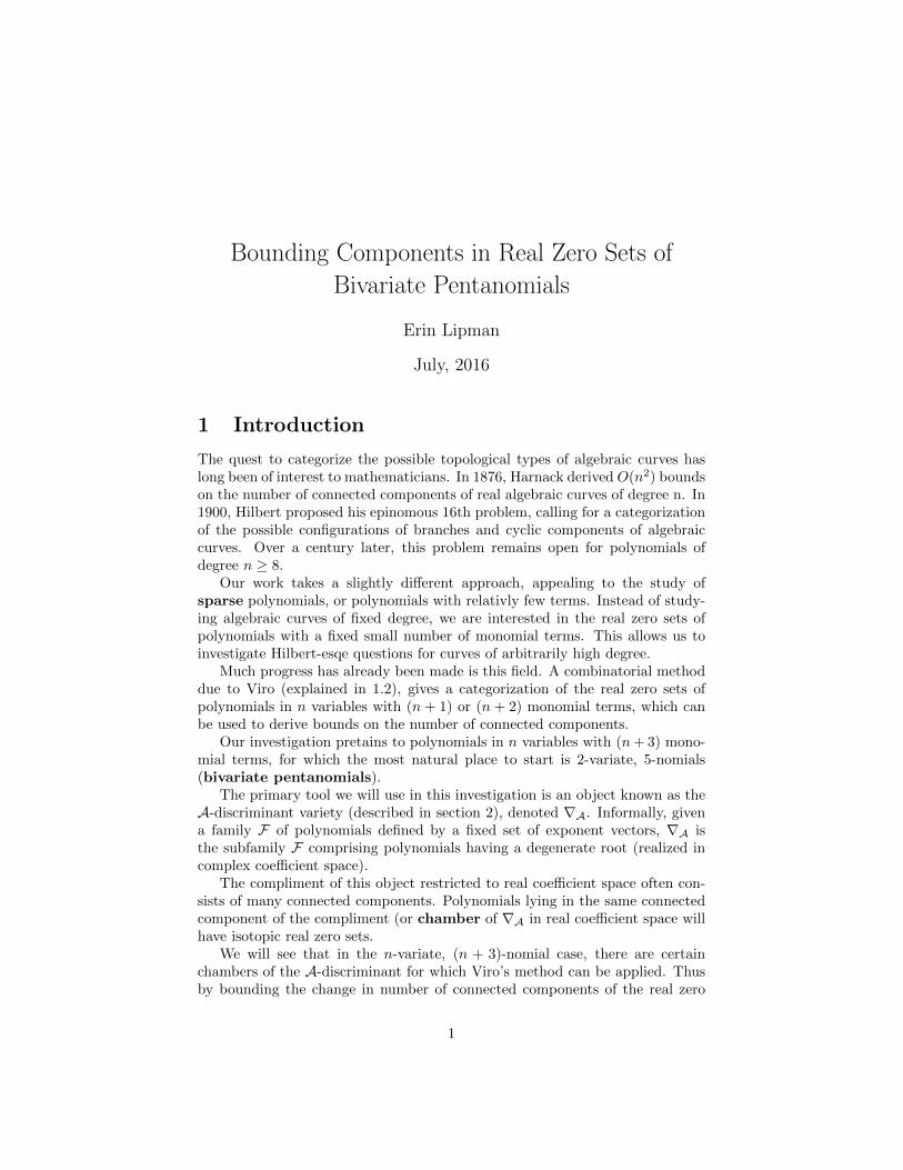
Definition 1.10. The Viro diagram of an honest n-variate, (n + 1)-nomial,V iro(f) is given by Conv(M), where M is the set of midpoints of edges ofSNewt(f) whose endpoints have opposite signs.

Example 1.11. Given f = 30− 11x+ 7y, figure 1, shows V iro(f), along withthe positive zero set of the polynomial. We notice that, viewing the hypotenuseof V iro(f) as lying at infinity, each object is connected and unbounded at oneend.

In general, the Viro diagram of an honest n-variate (n+ 1)-nomial is diffeo-morphic to the classical n-simplex, which exaplains why we need not considerchoice of triangulation as we will in higher cases.

Theorem 1.12. If f is an honest n-variate, (n+1)-nomial, V iro(f) is isotopicto the positive zero set of f .

3

Figure 1: Viro diagram and positive zero set for polynomial in example 1.11.

Figure 2: Viro diagrams correcponding to each of the triangulations forSNewt(g) (left) and SNewt(h) (right) from example 1.14

Viro’s method in the (n + 2)-nomial case works similarly, with the caveatthat we must first assign a triangulation to SNewt(f).

Definition 1.13. If f is an honest n-variate (n+2)-nomial, then given anytriangulation Σ, we define

V iroΣ(f) =⋃σ∈Σ

Conv(Mσ),

where Mσ is the set of midpoints of those edges of σ whose endpoints haveopposite signs.

Example 1.14. The signed Newton polygons for g = 30 − x + 7y − x2y2 andh = 30 − x + 7y − y4 each have two possible trianglations. The Viro diagramscorresponding to each of these is shown in figure 2.

Theorem 1.15. If f is an honest n-variate, (n + 2)-nomial, There exists atrianglation Σ of SNewt(f) such that V iroΣ(f) is isotopic to the positive zeroset of f .

In fact, given any such polynomial, we can use the A-discriminant to deter-mine exactly which triangulation to use. We will not, however, devote any moreattention to determining choice of triangulation since it is not relevant to theproject at hand.

Unfortunately, theorem 4.2 does not apply in general to the (n+ 3)-nomialcase. However, it does extend to the (n+3) case if we require that f correspondto a point in one of a certain subset of the chambers of the A-discriminantvariety corresponding to f . An exposition of this enormously useful object willbe the focus of the following section.

4

2 The A-Discriminant Variety

The A-discriminent is a generalization of the more familiar quadratic discrim-inant. We recall from high school algebra that a polynomial in the univariatetrinomial family

F = {ax2 + bx+ c : a, b, c ∈ C∗}

has a degenerate root exactly at the roots of the polynomial

∆(0,1,2)(a, b, c) = b2 − 4ac.

We will use this familiar example to demonstate the resultants method forcomputing the A-discriminant polynomial for an n-variate, (n+ k)-nomial.

We begin with the definition of the A-discriminant variety ∇A. Simplystated, given family F with support A, ∇A represents the set of polynomials inF having a nonzero degenerate root.

Definition 2.1. The A-discriminant variety of an n-variate (n+ k)-nomialwith support A = {a1, ..., an+k} ⊂ Zn is defined as the Zariski closure of:

∇A = {(c1, ...cn+k) ∈ P (C)n+k−1 :

∃ζ ∈ (C∗)n with f(ζ) = 0 and ∂f∂xi

(ζ) = 0 for all i ∈ {1, ..., n}}.

Theorem 2.2. If f, g ∈ F correspond to points in the same connected compo-nent of the compliment of ∇A in real coefficient space, then the real zero sets off amd g are isotopic.

2.1 The Resultants Method

Perhaps the most direct way to compute ∇A would be to find a polynomial ∆Awhose solution set is exactly ∇A. To do this, we will introduce the resultantsmethod for determining whether or not two polynomials have a common root.

Definition 2.3. Given polynomials f(x) = a0 + a1x + · · · anxn and g(x) =b0 + b1x + · · · bmxm, with ai, bi ∈ C and an, bm 6= 0, the Sylvester matrix off and g is defined to be the following (n+m)× (n+m) matrix:

Sylx(f, g) =

a0 a1 · · · am 0 0

0. . .

. . . 00 0 a0 a1 · · · amb0 b1 · · · bn 0 0

0. . .

. . . 00 0 b0 b1 · · · bn

.

5

A classical theorem describes how we can use the Sylvester matrix to com-pute ∆A.

Theorem 2.4. If f(x) = a0+a1x+· · · anxn and g(x) = b0+b1x+· · · bmxm, withai, bi ∈ C and an, bm 6= 0, then det(Sylx(f, g)) = 0 if and only if f(ζ) = g(ζ) = 0for some ζ ∈ C∗.

Thus if F is a univariate polynomial of degree d with support A, ∆A is givenby the determinant of the (2d− 1)× (2d− 1) matrix Sylx(f, f ′).

Example 2.5. In the case of our quadratic example, we derive the familiarformula, realizing that we may scale ∆A by the nonzero constant −a.

∆A = det

c b ab 2a 00 b 2a

= −a(b2 − 4ac).

This method can also be extended into a method for computing the A-discriminant polynomial for multivariate families.

While the resultants method is practical for this quadratic example, the sizeand complexity of computing a single Sylvester discriminant grows in the squareof the degree of F . Furthermore, ∆A for even a sparse polynomial often has anunmanagable number of terms.

We would like an alternate representation for ∇A that is both easy to com-pute and practical to use. We will find such a representation in the Horn-Kapranov uniformization.

2.2 Horn-Kapranov Uniformization

For a family F with support A = {a1, ..., an+k}, we define an (n+ 1)× (n+ k)matrix

A =

(1 · · · 1a1 · · · an+k

)and a corresponding (n+ k)× (k − 1) matrix B whose columns form a basis ofthe right null of A:

B =

b1...

bn+k

.

Theorem 2.6. ∇A can be parametrized in P (C)n+k−1 as the Zariski closure ofthe following:

ϕ(∇A) = {(b1 · λ)ta1 : · · · : (bn+k · λ)tan+k |λ ∈ P (C)k−2}.

6

We will denote the ith component of this parametriztion as γi.

Example 2.7. Consider the family

F = c1 + c2x+ c3y + c4x4y + c5xy

4.

Using

AB =

1 1 1 1 10 1 0 4 10 0 1 1 4

4 0−4 3−1 −31 −10 1

= 0,

we have

ϕ(∇A) = {(4λ1t(0,0) : (−4λ1+3λ2)t(1,0) : (−λ1−3λ2)t(0,1) : (λ1−λ2)t(4,1) : λ2t

(1,4)) : λ ∈ P (C)}

While ϕ(∇A) is easy to compute, its dimension depends on the number ofmonomial terms in F . In order to visualize ϕ(∇A) in a lower dimension, we willtake advantage of homogenaties to reduce F to a subfamily with coefficient spaceof dimension k− 1. We will also restrict our attention to the real component ofthe coefficient space.

We observe that if ζ ∈ (C∗)n, f(x1, . . . , xn)|ζ = 0 if and only if κf(α1x1, . . . , αnxn)|ζ =0.. Thus we may study the behavior of a subfamily of polynomials that will rep-resent equivalence classes of F .

Keeping F as in example 2.7, consider the subfamily F ′ = 1+x+y+ax4y+bxy4, which is the image of the map

[·] : F → F ′ by [f(x, y)] =1

c1f

(c1c2x,c1c3y

),

which in turn induces a map on the coefficient vectors

[·]∗ : P (C)5 → (C∗)2 by [(c1 : c2 : c3 : c4 : c5)]∗ =

(c41c4c42c3

,c41c5c2c43

).

In order to utilize the reduced A-discriminant, we will find it useful to con-sider the amoeba of its contour, meaning that we will plot the log-norm of itsreal component.

The reduced A-discriminant for our example with respect to the change ofvariables [·] is the following:

ϕ(∇A) =

(log

∣∣∣∣γ41γ4

γ42γ3

∣∣∣∣ , log ∣∣∣∣γ41γ5

γ2γ43

∣∣∣∣) ={(log∣∣∣ (4λ1)4(λ1−λ2)

(−4λ1+3λ2)4(−λ1−3λ2)

∣∣∣ , log ∣∣∣ (4λ1)4(λ2)(−4λ1+3λ2)(−λ1−3λ2)4

∣∣∣) : λ ∈ P (C)}

7

Figure 3: Reduced A-discriminant amoeba for F (right image zoomed in toshow cusps). In addition to the 3 clearly visible places where the discriminant’blows up’, the discriminant also extends infinitely along the negative x andnegative y axes.

2.3 Unfolding the Reduced A-Discriminant

We would like to be able to apply theorem 2.2 to ϕ(∇A), however in taking thelog norm, ϕ(∇A) is no longer homeomorphic to ∇A. To preserve the bijection,we instead take the log norm of each quadrant of the coefficient space separately.

Definition 2.8. Let F be a family of n-variate, (n+ k)-nomials.For (σ1, . . . , σk−1) ∈ {±1}k−1, then we define

ϕ(∇A)(σ1,...,σk−1) = ϕ(∇A)|λ(σ1,...σk−1),

where

λ(σ1,...σk−1) = {λ ∈ P (R)k−1 :ϕi(λ)

|ϕi(λ)|= σi for i ∈ {1, . . . , k − 1}.,

and ϕ is the map identical to ϕ except that we refrain from taking the lognorm.

We observe that ϕ is undefined exactly where bi · λ = 0 for some row biof B. Thus in the (n + 3)-nomial case, it is undefined for at most (n + 3)distinct values of λ ∈ P ((R))- near these values, the function goes off to infinityin some direction. Thus ϕ is the union of ≤ 5 (smooth) unbounded connectedcomponents. Since in between these values, ϕ is continuous (and nonzero),each of its connected components is contained completely in ϕ(∇A)(σ1,...,σk−1)

for some σ1, . . . , σk−1.It is often helpful to visualize P ((R)) as the upper half circle (with the 2

endpoints identified).

8

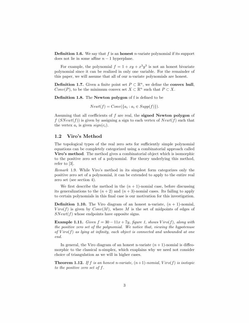
Figure 4: B matrix and annotated domain for example 2.9

Example 2.9. Continuing again our example

F = 1 + x+ y + ax4y + bxy4,

figure 4 shows the domain of ϕ. The marked points represent the values of λ forwhich ϕ ’blows up’, and the ordered pairs of signs denote which quadrant of thereduced ϕ contains the image of this portion of the domain.

Figure 5 shows the signed reduced A-discriminant for mathcalF .

ϕ(−,+) ϕ(−,+)

ϕ(−,−) ϕ(+,−)

Figure 5: The signed reduced A-discriminant corresponding to example 2.9.

Having established in detail the machinary needed to work with the A-discriminant,we proceed to prove the main theorem regarding change in number of comnectedcompoents of a polynomial as we cross between chambers.

9

3 Proof of Main Theorem

The proof of the theorem is intuitive and the following section mainly amountsto an untangling of subtleties - the outline of the argument is as follows.

Consider a family F of the form described in theorem 1.2 (main theorem).

1. Given a polynomial f on the boundary between two chambers of the A-discriminant for F , there exists constant ε such that f + ε and f − ε lie inopposite chambers.

2. We can ensure that f has exactly one degenerate root and that at this root,the surface defined by f(x, y) attains either a local extremum or a saddlepoint.

3. Assuming that ε is sufficiently small, the cross sections of the surfacef(x, y) at f(x, y) = ±ε differ in number of (compact) connected compo-nents by at most 1.

Definition 3.1. We define the set of critical points of surface f(x, y) to be

W = {(x, y) ∈ R2 : ∂f(x,y)∂x = ∂f(x,y)

∂y = 0}. Define the z-coordinate projection

πz : W → R to be πz(x, y) = f(x, y). We refer to the image πz(W ) as the setof critical values of f .

Lemma 3.2. A surface f(x, y), where f(x, y) = 0 is a bivariate polynomail,has finitly many critical values, ie πz(W ) is finite.

Proof. By Sard’s theorem, we have that πx(W ) has Lebesgue measure zero in R.We now appeal to the theory of semi-algebraic sets (a superset of algebraic sets).The projection of a semialgebraic set is semialgebraic, and a semialgebraic set isthe finite union of points and open intervals. Thus a measure zero semi-algebraicset is a finite point set.

For a surface f(x, y), let δf(x,y) = min{|w| : w ∈ πz(W )}.Remark 3.3. Since topological type is constant within a chamber of the signedA-discriminant, it suffices to show that given any pair of adjacent chambers,the result holds for some pair of polynomials on opposite sides.

3.1 Generic properties of polynomials on ϕ(∇A)

Consider the surface defined by f(x, y) = 1 + x + y + axα1yα2 + bxβ1yβ2 . Ac-cording to the definition of πz(W ), (x, y) is a degenerate root of f exactly when(x, y, f(x, y) = 0) is a critical point. Henceforth we will refer to degenerate rootsas critical roots to premptivly avoid confusion with degenerate critical points.

The critical points of an algebraic surface in R3 come in several forms. Anondegenerate critical point is either a local extremum (maximum or minimum)

10

or a saddle point. Critical points can be categorized by studying the eigenvaluesof the Hessian matrix.

Definition 3.4. Given a c2 function f : Rn → R, the Hessian matrix of f isdefined as follows:

H(f) =

∂2f∂x2

1· · · ∂2f

∂x1∂xn...

. . ....

∂2f∂xn∂x1

· · · ∂2f∂x2n

Definition 3.5. A critical point x ∈ Rn is degenerate if

det(H(f)|x) = 0,

ie the Hessian is neither positive semidefinite nor negative semidefinite.

Before discussing generic properties, we define this notion of a generic prop-erty.

Definition 3.6. We say a property P is generic in Rn if it holds on thecompliment of an algebraic set - ie there exists an honest n-variate polynomialf such that P holds exactly when f = 0.

By showing that polynomials on the A-discriminant generically have non-degenerate critical roots, we will be able to assume without loss of generalitythat a critical root of such a polynomial is either a local extremum or a saddlepoint.

Theorem 3.7. Given family

F = {1 + x+ y + axα1yα2 + bxβ1yβ2},

where αi and βi are fixed integers, a generic point on ϕ(∇A) has exactly onecritical root. Furthermore, this critical root is a nondegenerate critical point.

Proof. F has A matrix

A =

1 1 1 1 10 1 0 α1 β1

0 0 1 α2 β2

,

whose null space is given by1− α 1− βα1 β1

α2 β2

−1 00 −1

,

11

where α = α1 + α2 and β = β1 + β2,and Hessian matrix

H(f) =

(aα2

1xα1−2yα2 + bβ2

1xβ1−2yβ2 aα1α2x

α1−1yα2−1 + bβ1β2xβ1−1yβ2−1

aα1α2xα1−1yα2−1 + bβ1β2x

β1−1yβ2−1 aα22xα1yα2−2 + bβ2

2xβ1yβ2−2

).

Recalling our definition of the A-discriminant, a point on ϕ(∇A) which isthe image of λ ∈ P (R) satisfies the following equation:

c ∗

1xy

axα1yα2

bxβ1yβ2

= λ1

1− αα1

α2

−10

+ λ2

1− ββ1

β2

0−1

,

where c is a real scaler accounting for the fact that λ lies in projective space,(x, y) is a critical root, and a, b are real coefficients.

Since P (R) can be represented as the set of lines through the origin in R2,we can identify λ by the ratio λ2

λ1. We begin by fixing λ2 = rλ1, eg λ1 = 1,

λ2 = r, and following though a series of implications.

→ c = 1− α+ r(1− β) depends linearly on r.

→ x = c−1(α1 + rβ1), and similarly y, is determined by r.

→ a = c−1( −1xα1 y

α2

), and similarly b, is also determined by r.

Both portions of the theorem follow immediately from these relations.Since (x, y) is determined by λ, a polynomial has multiple critical roots only

if it corresponds to a self intersection of ϕ. Since all intersections of ϕ aretransverse (see [5]), a generic point on ϕ has only one critical root.

Furthermore, assuming that λ · bi = 0 for all rows bi (otherwise ϕ is notdefined), det(H(f)|x,y) is a univariate polynomial equation in variable r. Thus,generically a critical root is nondegenerate.

3.2 The Proof

Let F = {c1+c2x+c3y+c4xα1yα2 +c5x

β1yβ2 : ci ∈ R} and suppose ϕ(∇A) ∈ R2

is the reduction of ∇A to the subfamily F ′ = {1 + x+ y + axα1yα2 + bxβ1yβ2 :a, b ∈ R}. by the followinf map:

[·] : F → F ′ by [f(x, y)] =1

c1f(c1c2x,c1c3y).

12

Definition 3.8. If quadrant ϕ(∇A)σ1,σ2 of the unfolded reducedA-discriminanthas chambers {V1, · · ·Vn}, then chambers Vi and Vj are adjacent if V i ∩ V jcontains the injective image of an interval. We will call V i ∩ V j the commonboundary of Vi and Vj .

In order to show that the theorem hold for all f, g : f ∈ Vi, g ∈ Vj, we beginby considering a polynomial

f = 1 + x+ y + σ1ea0xα1yα2 + σ2e

b0xβ1yβ2 (2)

corresponding to a point p=(a0, b0) on ϕ(∇A)σ1,σ2. We can assume without

loss of generality that f has exactly one critical root and that ∂ϕ2

∂ϕ1|p 6= β−1

α−1

(the second fact is clearly true since the second derivative of ϕ are genericallynonzero).

We consider the sum of f with the constant monomial ε, where we assume|ε|< min(1, δf ). Using our change of variables [·],

[f + ε] = 1 + x+ y + σ1ea0(1 + ε)α−1xα1yα2 + σ2e

b0(1 + ε)β−1xβ1yβ2 . (3)

Then the parametric curve of points corresponding to [f + ε] is

C = (log(ea0(1 + ε)α−1), log(eb0(1 + ε)β−1)), (4)

with constant slope ∂C2

∂C1= β−1

α−1 .Thus C crosses ϕ transversely at p, and for ε of sufficiently small absolute

value, we obtain [f + ε] ∈ Vi, [f − ε] ∈ Vj.It remains only to examine the change in number of connected components

as the cross section for f(x, y) changes from f + ε = 0 to f − ε = 0, assuming fhas a single nondgenerate critical root and the surface f(x, y)|ε−ε has no othercritical points.

It is a result of classical Morse theory that the topological type of the crosssection of a surface changes only at critical values (for more on CMT see e.g.[2]. Thus the cross sections of the restriction of f(x, y) to the domain with anopen neighborhood around the critical root are all isotopic.

An analysis of directional second derivatives illuminates the behavior aroundthe critical root. The behavior around a nondegenerate critical point is illustratedin figure 3.2.

If the root is a local extremum, varying the cross section in one directioncauses the genesis of a compact component, while varying it in the other directiondoes the reverse. Thus around a local extremum, Non(f) remains constant andComp(f) changes by exactly 1.

At a saddle point, taking cross-scetions ε above and below the critical point lo-cally give 2 distinct components that change their relative configuration as shownin 3.2. Non(f) stays constant and Comp(f) changes by 0 or 1 depending onwhether the two components are globally part of the same connected componentof the curve.

13

Figure 6: Change in local isotopy type of cross sections of f(x, y) as we cross acritical value.

4 Viro’s Method and Bounds on Connected Com-ponents

Figure 7: Viro diagrams for F(−,−) using 3 different triagulations

4.1 Bounds on Components for polynomials in Outer Cham-bers

We recall from 1.2 that Viro’s method applies to (n + 3)-nomials in certainchambers of the A-discriminant. We now make this more precise.

Definition 4.1. In the setting of (n+ 3)-nomials, an outer chamber is a con-nected components of ϕ having unbounded area. A non-outer chamber is an

14

inner chamber.

Theorem 4.2. If f is an honest n-variate, (n + 3)-nomial lying in an outerchamber of the corresponding A-discriminant variety, there exists a trianglationΣ of SNewt(f) such that V iroΣ(f) is isotopic to the positive zero set of f .

Figure 8: Classical and expanded signed Newton Polygon for F .

So to bound the number of components of real zero sets of certain families ofbivariate pentanomials, we first bound the number of components for polynomialsin the outer chambers, and the bound the ’depth’ of an arbitrary chamber.

We expand slightly on the version of Viro’s method described in section 1.2for the case where the exponents in our polynomial are positive. Instead of simplyusing the signed Newton polygon to characterize just the positive zero set, wereflect SNewt(f) across both the x and y axes, flipping the signs acordinglybased on the powers of x and y. We then assign a triagulation to the SNewt,and reflect this triangulation to the additional quadrants, constructing the Virodiagram as before. In this way we characterize the entire real zero set.

Figure 8 shows the classical and extended signed Newton polygons for

F(−.−) = {1 + x+ y − |a|x4y − |b|xy4}.

Figure 7 gives the Viro diagrams corresponding to F(−,−) under three distincttriangulations. By symmetry, these are comprehensive. From this we see thateach polynomial in the outer chamber of ϕ(−,−) has three, unbounded connectedcomponents. We also note that the number of unbounded connected componentsdoes not depend on choice of triangulation, but rather on the number of signalternations on the outer boundary of the extended SNewt.

The shape of the (extended) SNewt depends on the support of F , where asbefore we fix the first three support vectors to be ((0, 0), (1, 0), (0, 1)), with theremaining exponents being positive integers. Figure 9 illustrates each of thefive fundamentally different shapes for the Newton polygon and the maximumnumber of components for a corresponding Viro diagram. The blue vertices arethose that can be designated either positive of negative.

We summarize this figure in the following lemma.

15

(a)max Non: 5max Comp: 0sample poly:f = 1+x+y+ax5y8+bx8y5

(b)max Non: 3max Comp: 0sample poly:f = 1+x+y+ax5y5+bx8y8

(c)max Non: 2max Comp: 1sample poly:f = 1 + x+ y + ax5 + by8

(d)max Non: 3max Comp: 0sample poly:f = 1 + x+ y + ax5 + bx8y8

(e)max Non: 1max Comp: 0sample poly:f = 1 + x+ y + ax5 + bx8

Figure 9: Maximum components by shape of Newton Polygon

Lemma 4.3. Given a polynomial f ∈ {1+x+y+axα1yα2 + bxβ1yβ2}, for fixedαi, βi ∈ Z≥0,

Non(f) ≤ 5, Comp(f) ≤ 1, and Tot(f) ≤ 5.

4.2 Proof of Corollary

By the depth of a chamber Vi, we mean the minimum length of a path Vouter, . . . , Vi,where Vouter ranges over the outer chambers and sucsessive chambers are re-quired to be adjacent. E.g. an outer chamber has depth 1. We now provecorollary 1.4.

Consider again family F as in lemma 4.3. Then we have:

ϕ =

(γα−1

1 γ4

γα12 γα2

3

,γβ−1

1 γ5

γβ1

2 γβ2

3

),

16

where γi are linear form on λ ∈ P (R).

Figure 10: Domain for F with some arcs marked with quadrant of their imagein signed ϕ. ϕ is with respect to B as above.

When γ4 = 0, ϕ is undefined. Also, since γ4 has multiplicity 1 in ϕ1, thisquantity changes sign to either side of the value of λ associated with γ4 = 0.Thus the portions of the domain on either side of γ4 = 0 lie in distinct quadrantsof the signed A-discriminant. The same reasoning applies to γ5 with regards toϕ2.

If we verify that the zeros for γ4 and γ5 are adjacent in the domain, weensure that at least 3 quadrants of signed ϕ are non-empty. This would alsoimply that if a given quadrant contains the images of exactly 3 arcs, then thesearcs are adjacent. Using the same B matrix as in section 3, this is indeed thecase. Figure 10 clarifies this notion.

Figure 11: Extremal configuration of arcs in quadrant of ϕ. Chambers arelabelled with depth.

Having established that a given quadrant contains at most three arcs, itis straightforward to charactarize the type of extremal example that maximizechamber depth. To do this, we recall several following results from [5]:

1. The reduced A discriminant for an n variate (n + 3)-nomial has at most2 cusps. We partition each arc into sub-arcs at the cusps. We then have,in the extremal case, 5 sub-arcs.

2. A subarc has no points of self-intersection.

3. Adjacent sub-arcs cannot intersect.

17

These 3 facts bound the number of intersections in the extremal case to atmost 6. Figure 11 illustrates the general form of a chamber containing 3 arcsand 5 sub-arcs. From this it is combinatorially evident that the depth of anarbitrary chamber does not exceed 3. It is easy to check that the non-extremalcases do not affect this bound.

Combined with the lemma from 4.1, this gives us the corollary.

4.3 Some Final Remarks

1. The author suspects that that the processes used to prove the theorem andcorollary, if not the results themselves, could with minimal modification beapplied to arbitrary families of bivariate pentanomials. In particular, anarbitrary family of bivariate pentanomials is equivilant to a family of theform

F = {1 + xκ1 + yκ2 + axα1yα2 + bxβ1yβ2}.for some αi, βi, γi ∈ Z.

2. We are not certain whether our bound on the number of compact (or total)components is sharp. Finding extremal examples with 2 or 3 compact com-ponents would be a worthwhile pursuit. The previous subsection’s analysisof sign changes across the domain provides some insight into where tolook.

References

[1] I. M. Gelfand, M. M. Kapranov, and A. V. Zelevinsky. Discriminants,Resultants, and Multidimensional Determinants. Springer, New York, 1994.

[2] M. W. Hirsch. Differential Topology. Springer, New York, 1997.

[3] I. Itenberg, G. Mikhalkin, and E. Shustin. Tropical Algebraic Geometry.Birkhauser Verlag AG, Berlin, 2009.

[4] D. Perrucci. Some bounds for the number of components of real zero sets ofsparse polynomials. Discrete and Computational Geometry, 2005.

[5] K. A. Rusek. A-discriminant varieties and amoebae. PhD thesis, Texas AMUniversity, 2013.

Acknowledgments

This reseach was supported by the NSF as part of the REU program at TexasA&M University. The author would like to thank Dr. J. Maurice Rojas forhis advising and mentorship, as well as Alperen Ergur, Kaitlyn Phillipson, andYuyu Zhu. The author would also like to thank colleague Lucy Yang for herinsight throughout the summer.

18