Embed Size (px)
Citation preview
BOUNDING THE DECAY OF P-ADIC OSCILLATORY INTEGRALS WITH A
CONSTRUCTIBLE AMPLITUDE FUNCTION AND A SUBANALYTIC PHASE FUNCTION
BOUNDING THE DECAY OF P -ADIC OSCILLATORY INTEGRALS WITH A
CONSTRUCTIBLE AMPLITUDE FUNCTION AND A SUBANALYTIC PHASE FUNCTION
By
HOSSEIN TAGHINEJAD, M.Sc.,B.Sc.
A Thesis
Submitted to the School of Graduate Studies
in Partial Fulfillment of the Requirements
for the Degree
Doctor of Philosophy
McMaster University
c© Copyright by Hossein Taghinejad, October 2016
DOCTOR OF PHILOSOPHY (2016) MCMASTER UNIVERSITY
(Mathematics & Statistics) Hamilton, Ontario
TITLE: BOUNDING THE DECAY OF p-adic OSCILLATORY
INTEGRALS WITH A CONSTRUCTIBLE AMPLI-
TUDE FUNCTION AND A SUBANALYTIC PHASE
FUNCTION
AUTHOR: Hossein Taghinejad
M.Sc.,B.Sc.
SUPERVISOR: Dr. Deirdre Haskell
NUMBER OF PAGES: 1, 64
ii

To my mother, father and brother
Abstract
We obtain an upper bound for oscillatory integrals of the form∫Rmv
f(x)ψ(y.φ(x))|dx| where ψ is
an additive character, φ : Rmv → K is an analytic map satisfying the hyperplane condition and
f ∈ C(Rmv ) is integrable. Igusa, Lichtin and Cluckers have proved that we can find the decay rate
for such oscillatory integrals with certain conditions on f and φ. In this thesis we generalize those
results by imposing the hyperplane condition on φ.
iv
Contents
Abstract iv
1 Introduction 1
2 Valued fields and the model-theoretic setting 3
3 Haar measure and p-adic integration 12
4 Cell decomposition and constructible functions 20
5 Additive characters 28
6 p-adic Van Der Corput’s Lemma 36
7 Main Theorem 50
Bibliography 62
v
Ph.D. Thesis - H. Taghinejad McMaster - Mathematics & Statistics
Chapter 1
Introduction
In this thesis, we want to study a certain property of some specific p-adic integrals, namely the
decay rate of p-adic oscillatory integrals of the form
∫Rmv
f(x)ψ(φ(x).y)|dx|
in which Rv is the valuation ring of a local p-adic field, φ : Rmv → K is an analytic function, f(x)
is a constructible function on Rmv (f ∈ C(Rm
v )),|dx| is the Haar measure and ψ is an additive
character. We call f the amplitude and φ the phase function. The main theorem we prove in this
thesis is:
Theorem 1.1. Let φ : Rmv → K be an analytic map satisfying the hyperplane condition. Let
f ∈ C(Rmv ) be integrable and suppose ψ is an additive character. Let ε > 0. Then there are real
numbers s < 0 and c > 0 such that
|∫Rmv
f(x)ψ(y.φ(x))|dx|| ≤ cmin{1, |y|s}+ ε
for all y ∈ K×. Moreover, s does not depend on ε while c does.
The Vinogradov symbol � has its usual meaning, namely that for complex valued functions f
and g with g taking non-negative real values f � g means |f | ≤ cg for some constant c.
This theorem has a long history. In his book [14] of 1978, Igusa proves Theorem 1.1 in the case
that f(x) = 1 for all x and φ : Km → K is a nonconstant homogeneous polynomial and then he
1
Ph.D. Thesis - H. Taghinejad McMaster - Mathematics & Statistics
used the results to give a nice description of the generalized Gaussian sum of the p-adic oscillatory
integrals. He formulates the problem of generalizing this to the case of homogeneous polynomial
maps φ : Km → Kr for r > 1. By a very careful analysis of embedded resolutions of f , Lichtin [17]
is able to prove Igusa’s version of Theorem 1.1 in the case that φ : Km → K2 is a dominant map
(a map whose image is Zariski dense in the co-domain) whose coordinate maps are polynomial.
By using cell decomposition, Cluckers [5] proves Theorem 1.1 in the case that φ : Rmv → Kr is a
restricted power series such that φ(Rmv ) has nonempty interior in Kr, for arbitrary r. The goal
of this thesis is to replace the dominancy condition by the hyperplane condition which is a more
general case.
The hyperplane condition is defined as :
Definition 1.2. Let X ⊆ Kr be a subanalytic set. We say that a measurable function φ : X ×
Km → Kn satisfies the hyperplane condition over X if for every x ∈ X and every affine hyperplane
H in Kn, the set {y ∈ Km : φ(x, y) ∈ H} has measure zero.
The hyperplane condition is an adaptation of a condition from Stein’s book [23], to the context
of analytic maps instead of C∞ maps. Stein also proved decay results under this hyperplane
condition (but with compactly supported smooth amplitudes). In [8], Cluckers and Miller prove
Theorem 1.1 in the case of a real field by using real analytic tools such as the van der Corput
lemma and its corollaries and a specific version of cell-decomposition. In this thesis, we prove a
further modification of the version of Van Der Corput’s lemma on the p-adic fields which is proved
by Cluckers in [7].
In the first six chapters we discuss the requirements to proving the main theorem. In chapter
two, we review some basic definitions and theorems regarding valued fields and subanalytic sets.
We also discuss the model theoretic setting for studying p-adic integration. In chapter three, we
discuss Haar measure and p-adic integration. In the fourth chapter, we state cell decomposition
and we verify some properties of constructible functions. In chapter five, we review some properties
of additive characters. In chapter six, we state Van Der Corput’s lemma proved by Cluckers and
we prove a generalized version of that lemma. In the last chapter, we restate the main theorem
and we prove it.
2
Ph.D. Thesis - H. Taghinejad McMaster - Mathematics & Statistics
Chapter 2
Valued fields and the model-theoretic
setting
In this chapter, we present the classic definitions and theorems about valued fields and local fields.
We also discuss the required model-theoretic setting for studying p-adic integration. We refer the
reader to [15],[12],[25] and [10] for more details.
Let Γ be an ordered abelian group. We define a valuation v on a field K to be a surjective map
v : K → Γ ∪ {∞} satisfying the following axioms:
• v(x) =∞⇔ x = 0;
• v(xy) = v(x) + v(y);
• v(x+ y) ≥ min{v(x), v(y)}
for all x, y ∈ K. The set
Rv := {x ∈ K|v(x) ≥ 0}
is a valuation ring of K, i.e., a subring of K such that for all x ∈ K× either x ∈ Rv or x−1 ∈ Rv.
The set of non-units Mv := {x ∈ K|v(x) > 0} forms a maximal ideal of Rv; in fact, the only such.
We call the quotient Kv := Rv/Mv the residue field of v.
An example is given by the p-adic valuation, where p is any prime number. We define the
3
Ph.D. Thesis - H. Taghinejad McMaster - Mathematics & Statistics
p-adic valuation v : Q→ Z ∪ {∞} by v(0) =∞ and
v(prm
n) = r
where m,n ∈ Z \ {0} are not divisible by p. Clearly, the valuation ring Rv is the localization Z(p)
of the ring Z at the prime ideal pZ and the maximal ideal Mv is pZ(p). Thus the residue field is
isomorphic to the finite field Fp. We define a metric on Q by using the p-adic norm |x|p = p−v(x).
If Γ ⊆ R, the valution v induces an ultrametric on K by |x − y|v = e−v(x−y) that satisfies the
ultrametric inequality
|x+ y|v ≤ max{|x|v, |y|v}.
We call the topology induced by this metric the v-topology and it has the following properties:
• For each a ∈ K and γ ∈ Γ we define
Uγ(a) = {x ∈ K : v(x− a) > γ)}.
These sets form a basis of open neighborhoods of a.
• The sets {x ∈ K : v(x− a) ≥ γ}, {x ∈ K : v(x− a) ≤ γ},{x ∈ K : v(x− a) = γ} and Uγ(a)
are both open and closed.
• The field operations are continuous with respect to this metric topology.
A valuation v of K is called discrete if Γ is a discrete subgroup of (R,+); that is, if Γ = Zβ for
some real number β ≥ 0. Since in this thesis we just need to deal with discrete valuations, from
now on we assume that v is a discrete valuation on K.
A sequence of points, x1 , x2 , x3 , . . . , in K converges to x ∈ K in the v-topology , that is
limn→∞
xn = x
if and only if limn→∞ v(xn−x) =∞. When this is so, then limn→∞ v(xn) = v(x). In fact, if x 6= 0,
then v(xn) = v(x) for all sufficiently large n. A sequence x1 , x2 , x3 , . . . , in K is called a
4
Ph.D. Thesis - H. Taghinejad McMaster - Mathematics & Statistics
Cauchy sequence in the v-topology when
v(xn − xm)→∞, as m,n→∞.
A convergent sequence is, of course, a Cauchy sequence, but the converse is not necessarily true.
The valuation v is called complete if every Cauchy sequence in the v-topology converges to a point
in K. If v is complete then the infinite sum
∞∑n=1
xn = limi→∞
i∑n=1
xn
converges in K if and only if v(xn)→∞, as n→∞.
Let K ′ be an algebraic extension field of K, and v′ a valuation of K ′. Let v′|K denote the
function on K, obtained from v′ by restricting its domain to the subfield K. Then v′|K is a
valuation of K, and we call it the restriction of v′ to the subfield K. On the other hand, if v is a
valuation of K, any valuation v′ on K ′ such that v′|K = v is called an extension of v to K ′.
Let (K ′, v′) be an extension of (K, v). It is easy to see that the residue field of v is naturally
embedded in the residue field of v′. On the other hand, v′|K = v also implies that Γ is a subgroup
of Γ′. Let
e = [Γ′ : Γ], f = [K ′v′ : Kv]
where [Γ′ : Γ] is the group index and [K ′v′ : Kv] is the degree of the extension K ′v′/Kv. The integers
e and f are called the ramification index and the residue degree of the extension v′/v, respectively.
The following proposition is a fundamental result on the extension of valuations:
Theorem 2.1. Let v be a complete valuation of K and let K ′ be an algebraic extension of K. Then
v can be uniquely extended to a valuation v′ of K ′. If in particular, K ′/K is a finite extension,
then v′ is also complete, and
v′(x′) =1
nv(NK′/K(x′))
for all x′ ∈ K ′, where n = [K ′ : K] is the degree and NK′/K is the norm of the extension K ′/K.
Proof. We refer the reader to van der Waerden, [25].
5
Ph.D. Thesis - H. Taghinejad McMaster - Mathematics & Statistics
Let v be a valuation of K, not necessarily complete. It is well known that there exists an
extension field K ′ of K and an extension v′ of v on K ′ such that v′ is complete and K is dense
in K ′ in the v′-topology of K ′. Such a field K ′ is called a completion of K with respect to the
valuation v. By the definition, each x′ ∈ K ′ is the limit of a sequence of points, x1 , x2 , x3 , . . .
, in K in the v′-topology:
x′ = limn→∞
xn.
Then v′(x′) = limn→∞ v(xn) and hence if x′ 6= 0, then v′(x′) = v(xn) for all sufficiently large n. It
follows that the valued group does not change.
Let π0 ∈ K be an element with least positive valuation. Any such element π0 is called a prime
element of K. Let
Mnv = (πn0 ) = Rvπ
n0 = {x ∈ K : v(x) ≥ nv(π0)}
be the ideal of Rv generated by πn0 for n ∈ Z. Fix A a complete set of representatives of the residue
field of K. The following theorem can be found in [15].
Theorem 2.2. Each nonzero x ∈ K can be uniquely expressed in the form
x =∞∑n=i
anπn0
where an ∈ A for all n and v(x) = i. We call x =∑∞
n=i anπn0 the p-adic expansion of x. We can
obtain the p-adic expansion of 0 ∈ K by choosing all coefficients to be zero.
Proof. The uniqueness is easy to verify. Without loss of generality, we assume x 6= 0, v(x) = i <∞.
Now, by the definition of A,
Rv = A+Mv = {a+Mv : a ∈ A}.
Since Mnv = {x ∈ K : v(x) ≥ nv(π0)} for n ∈ Z, it follows that
Mnv = Aπn0 +Mn+1
v = Aπn0 + Aπn+10 + ...+ Aπm0 +Mm+1
v
for all m ≥ n. As x ∈ M iv, we see that there exists a sequence of elements in A, ai, ai+1, ..., such
6
Ph.D. Thesis - H. Taghinejad McMaster - Mathematics & Statistics
that
x ≡j∑n=i
anπn0 ( mod M j+1
v )
for any j ≥ i. It then follows that
x = limj→∞
j∑n=i
anπn0 =
∞∑n=i
anπn0 .
Moreover every such series∑∞
n=i anπn0 converges if v is a complete valuation on K since
v(anπn0 )→∞.
Let A∞ denote the set of all sequences (a0, a1, a2, ...), where an are taken arbitrarily from the
set A defined above. Thus A∞ is the set-theoretical direct product of the sets An = A for all n ≥ 0:
A∞ =∞∏n=0
An.
Introduce a topology on A∞ as the direct product of discrete spaces An, n ≥ 0.
Corollary 2.3. The map
(a0, a1, a2, ...)→∞∑n=0
anπn0 ,
defines a homeomorphism of A∞ onto the valuation ring Rv of (K, v).
Proof. Let x =∑anπ
n0 and y =
∑bnπ
n0 where an, bn ∈ A. Then it is easy to verify that for any
integer i,
v(x− y) ≥ i⇐⇒ an = bn for all n < i.
This fact shows that the map is bijective and Theorem 2.2 implies that it is a homeomorphism.
Corollary 2.4. K is a locally compact field in its v-topology.
Proof. Since A∞ is a compact space, by Corollary 2.3, Rv is compact and hence K is locally
compact.
7
Ph.D. Thesis - H. Taghinejad McMaster - Mathematics & Statistics
Next, we want to review some important properties of the valued field extensions. Let (K ′, v′)
be a complete extension of the complete valued field (K, v). We discussed before that Kv can be
naturally embedded into K ′v. Let w1, ..., ws be any finite number of elements in K ′v, which are
linearly independent over Kv, and for each i, 1 ≤ i ≤ s, choose an element ξi in R′v′ that belongs
to the residue class wi in K ′v. Fix a prime element π′0 ∈ K ′ and let
ηij = ξiπ′jo ,
for 1 ≤ i ≤ s and 1 ≤ j ≤ e where e is the ramification index of the extension K ′/K.
Theorem 2.5. With the notation from previous paragraph
1. Let x′ =∑xijηij with xij ∈ K. Then
v(x′) = min{ev(xij) + j : 1 ≤ i ≤ s and 0 ≤ j < e},
and the elements ηij are linearly independent over K.
2. If the residue degree is finite then the elements ηij form a basis of K ′ over K and
[K ′ : K] = ef.
Proof. We refer the reader to [15].
The following corollary can be easily proved by using Theorem 2.5:
Corollary 2.6. Let (K ′, v′) be a complete extension of the complete valued field (K, v) with [K ′ :
K] = n. Suppose {z1, ..., zn} is basis of K ′ over K. Then the map
(x1, ..., xn) 7−→n∑i
xizi
defined from Kn into K ′ is a topological isomorphism.
The following lemma is well known as Hensels lemma and it plays an important role in this
thesis. From now on, we assume the K is a complete valued field.
8
Ph.D. Thesis - H. Taghinejad McMaster - Mathematics & Statistics
Lemma 2.7. Let g ∈ Rv[x] be a polynomial and let a0 ∈ Rv be such that v(g(a0)) > 2v(g′(a0)).
Then there exists some a ∈ Rv with g(a) = 0 and v(a− a0) > v(g′(a0)).
Proof. We refer the reader to [12].
If g(x) = c0 + c1x + ... + cnxn ∈ Rv[x] then by g(x) we mean c0 + c1x + ... + cnx
n where ci is
the residue class corresponding to ci. The next corollary is an easy consequence of Lemma 2.7.
Corollary 2.8. Suppose g ∈ Rv[x] such that g has a simple root a0 in the residue class Kv. Then
g has a zero a ∈ Rv such that a = a0.
We write Pn = {yn : y ∈ K×} for the collection of n-th powers in K× = K \ {0}. By
Corollary 2.8, each Pn has finite index when we consider it as a subgroup of the multiplicative
group K×. The following lemma shows a relation between being an element of Pn and the way we
can express that element as a convergent series (Theorem 2.2). By using the following lemma we
can easily prove that Pn is an open subset of K for all n.
Lemma 2.9. Let A be a complete set of representatives of the residue field of K. Let x =∑n≥i anπ
n0 ∈ K where an ∈ A for all n and v(x) = i ∈ Z. For m ∈ N, x ∈ Pm if and only
if ai = bm for some b ∈ K and m|v(x) = i.
Proof. Suppose x ∈ Pm. Then there is y ∈ K such that x = ym and hence v(x) = mv(y). Thus
m|v(x).
Let y =∑
n≥j bnπn0 where bn ∈ A for all n and v(y) = j ∈ Z. Then aiπ
i0 = bmj π
mj0 and hence ai = bmj .
Now suppose ai = bm for some b ∈ K and m|v(x) = i. We want to find y =∑
n≥j bnπn0 ∈ K
such that x = ym. Let j = v(x)m
and let bj = b. We can then find all subsequent bns for n > j
recursively.
Now we want to discuss the model-theoretic setting required for our purpose. Let La (a
for “algebraic”) be the language consisting of the binary operation symbols + and ., the unary
operation symbol −, the constant symbols 0 and 1, and the relation symbols Pn for all n > 1.
We consider K as an La–structure using the natural interpretations of the symbols of La. In [19],
Macintyre proved that K has elimination of quantifiers in La.
9
Ph.D. Thesis - H. Taghinejad McMaster - Mathematics & Statistics
For x = (x1, ..., xm), let K{x} be the ring of restricted power series over K in the variables x;
it is the ring of power series∑aix
i in K[[x]] such that |ai| tends to 0 as |i| → ∞. Equivalently,∑aix
i ∈ K{x} if∑aix
i is convergent on Rmv . Here we use the multi-index notation where
i = (i1, ..., im), |i| = i1 + ... + im and xi = xi11 ...ximm . For x0 ∈ Rm
v and f =∑aix
i ∈ K{x} the
series∑aix
i0 converges to a limit in K, thus, one can associate to f a restricted analytic function
given by
f : Km → K : x 7→
∑aix
i0, if x ∈ Rm
v ;
0, else.
We let Lan be the first order language consisting of the symbols of La together with an extra
function symbol f for each restricted analytic function associated to restricted power series in⋃mK{x1, ..., xm} and −1, the inverse operator on K with the convention 0−1 = 0. We consider
K as an Lan-structure using the natural interpretations of the symbols of Lan. In [10], Denef and
van den Dries proved that Zp admits quantifier elimination in this language and thus it follows
that K admits quantifier elimination in this language too. To describe the definable subsets of K
in this language we need to introduce the concept of D-function. Cluckers [6] gives the following
definition of D-functions:
Definition 2.10. A D-function is a function Km → K for some m ≥ 0, obtained by repeated
application of the following rules:
1. for each f ∈ K{x1, ..., xm}, the associated restricted analytic function x 7→ f(x) is a D-
function;
2. for each polynomial f ∈ K[x1, ..., xm], the associated polynomial function f(x) is a D-
function;
3. the function x 7→ x−1, where 0−1 = 0 by convention, is a D-function;
4. for each D-function f in n variables and each D-functions g1, ..., gn in m variables, the
function f(g1, ..., gn) is a D-function.
Now it is easy to see what the definable subsets of K look like:
10
Ph.D. Thesis - H. Taghinejad McMaster - Mathematics & Statistics
Definition 2.11. X ⊆ Km is a subanalytic set if X is definable in Lan. For A ⊆ Km, we call
f : A→ Kn a subanalytic map if its graph is subanalytic.
By using quantifier elimination and an inductive construction we can see that X is subanalytic
if X is a boolean combination of the sets {x ∈ Km | f(x) = 0} or {x ∈ Km | g(x) ∈ Pn}, where
the functions g and f are D-functions and n > 0. We refer to [10] for more details on the inductive
construction of subanalytic sets.
11
Ph.D. Thesis - H. Taghinejad McMaster - Mathematics & Statistics
Chapter 3
Haar measure and p-adic integration
In this chapter, we state the theorem related to the existence of Haar measure for an arbitrary
locally compact topological group. Next, we state and prove some properties of Haar measure which
we need to prove the main theorem in this thesis. Moreover, we define the p-adic integration and
prove some properties related to calculating p-adic integrals. We refer the reader to [21],[20],[16]
and [22] for more details.
We first recall a sequence of fundamental definitions from analysis that culminate in the defi-
nition of a Haar measure. A collection M of subsets of a set X is called a σ-algebra if it satisfies
the following conditions:
• X ∈M.
• If A ∈M, then Ac ∈M, where Ac denotes the complement of A in X.
• Suppose that An ∈M(n ≥ 1), and let A = ∪An. Then A ∈M.
It follows from these axioms that the empty set is in M and that M is closed under finite and
countably infinite intersections. A set X together with a σ-algebra of subsets M is called a
measurable space. If X is moreover a topological space, we may consider the smallest σ-algebra B
containing all of the open sets of X. The elements of B are called the Borel subsets of X.
A positive measure µ on an arbitrary measurable space (X,M) is a function µ : M→ R≥0∪{∞}
12
Ph.D. Thesis - H. Taghinejad McMaster - Mathematics & Statistics
that is countably additive; that is,
µ(∞⋃n=1
An) =∞∑n=1
µ(An)
for any family {An} of disjoint sets in M. In particular, a measure defined on the Borel sets of X
is called a Borel measure.
Let µ be a Borel measure on a locally compact Hausdorff space X, and let E be a Borel subset
of X. We say that µ is outer regular on E if
µ(E) = inf{µ(U) : E ⊆ U,U open}.
We say that µ is inner regular on E if
µ(E) = sup{µ(K) : K ⊆ E,K compact}.
A Radon measure on X is a Borel measure that is finite on compact sets, outer regular on all Borel
sets, and inner regular on all open sets. One can show that a Radon measure is, moreover, inner
regular on σ-finite sets (that is, countable unions of µ-measurable sets of finite measure).
Let G be a locally compact Hausdorff topological abelian group and let µ be a Borel measure
on G. We say that µ is translation invariant if for all Borel subsets E of G,
µ(sE) = µ(Es) = µ(E)
for all s ∈ G.
Definition 3.1. Let G be a locally compact Hausdorff topological abelian group. Then a Haar
measure on G is a nonzero Radon measure µ on G that is translation-invariant.
Theorem 3.2. Let G be a locally compact Hausdorff topological abelian group. Then G admits a
Haar measure. Moreover, this measure is unique up to a scalar multiple.
Proof. For a thorough proof of existence and uniqueness, see [21].
13
Ph.D. Thesis - H. Taghinejad McMaster - Mathematics & Statistics
Proposition 3.3. Let G be a locally compact topological abelian group with a nonzero Haar measure
µ. Then:
1. µ is positive on all nonempty open subsets of G.
2. µ(G) is finite if and only if G is compact.
Proof. 1. Since µ is not identically zero, by inner regularity there is a compact set K such that
µ(K) is positive. Let U be any nonempty open subset of G. Then from the inclusion
K ⊆⋃s∈G
sU
we deduce that K is covered by a finite set of translates of U, all of which must have equal
measure. Since µ(K) > 0, µ(U) > 0.
2. If G is compact, then certainly µ(G) is finite by definition of a Haar measure. To establish
the converse, assume that G is not compact. Let K be a compact set whose interior contains
the identity element, e (there is such a K since G is locally compact). Then no finite set
of translates of K covers G (which would otherwise be compact), and there must exist an
infinite sequence {sj} in G such that
sn /∈⋃j<n
sjK.
Now suppose W ⊆ K is an open neighborhood of e. Since . : G × G → G (. is the group
operation) is continuous, there is an open neighborhood of e, U ⊆ W , such that U = U−1
and UU ⊆ W .
We claim that the translates sjU(j ≥ 1) are disjoint, from which it follows at once from (1)
that µ(G) is infinite. To prove the claim, suppose for i < j we have siu = sjv where u, v ∈ U .
Then sj = siuv−1, since U is symmetric and UU ⊆ K. But this contradicts the fact that
sj /∈⋃i<j siK.
The following theorem states the property of Haar measure which is called continuity.
14
Ph.D. Thesis - H. Taghinejad McMaster - Mathematics & Statistics
Theorem 3.4. Let G be a locally compact topological abelian group with a Haar measure µ. Suppose
(A1, A2, ...) is a sequence of Borel subsets of G. Then
• If the sequence is increasing then
µ(∪∞i=1Ai) = limn→∞
µ(An).
• If the sequence is decreasing and µ(A1) <∞ then
µ(∩∞i=1Ai) = limn→∞
µ(An).
Now we want to define Haar integration. Let G be a locally compact topological abelian group
with a Haar measure µ. Let S ⊆ G be a Borel set and let χS be its characteristic function. We
define ∫G
χSdµ := µ(S).
Now suppose s =∑k=n
k=1 akχSk where Sk is a Borel subset of G and aks are real numbers for all k.
We call s a simple function. Suppose s is a non-negative simple function. We define
∫G
sdµ :=k=n∑k=1
akµ(Sk).
Now suppose f : G→ [0,+∞] is a measurable function. Let Tf = {s : 0 ≤ s ≤ f and s is simple}
The integral of f over G is defined as:
∫G
fdµ := sups∈Tf
∫G
sdµ.
If f is any measurable real-valued function on G we define:
∫G
fdµ =
∫G
f+dµ−∫G
f−dµ
15
Ph.D. Thesis - H. Taghinejad McMaster - Mathematics & Statistics
where f+ and f− are measurable and represent the positive and negative part of f, respectively:
f+(x) = max(+f(x), 0) f−(x) = max(−f(x), 0).
If E is a Borel subset of G then we define:
∫E
fdµ :=
∫G
χEfdµ
A nonnegative measurable function f is called integrable if its integral∫Gfdµ is finite. An
arbitrary measurable function is integrable if f+ and f− are each integrable.
Now suppose h : G→ C is a complex-valued function. We define:
∫G
hdµ =
∫G
Re(h)dµ+ i
∫G
Im(h)dµ
where Re(h) and Im(h) are the real and imaginary part of h respectively.
The next theorem is the analogue to the Lebesgue integrability of continuous functions with
compact support in the real case:
Theorem 3.5. Any continuous function f : G→ C with compact support is µ-integrable.
Let G be a locally compact topological abelian group with a Haar measure µ. The next
proposition combines the Haar integration with being translate-invariant of Haar measure:
Proposition 3.6. Let G be a locally compact topological abelian group with a Haar measure µ.
Let f : G→ C be a µ-integrable function. Then for every g ∈ G
∫G
f(x)dµ =
∫G
f(gx)dµ.
Proof. The statement is clear for characteristic and simple functions by using translate-invariance
of µ. For a nonnegative measurable function the statement is obvious by using the integral defini-
tion and the fact that the claim is true for simple functions. Now the statement is clear for any
µ-integrable function by using the previous fact for f+ and f−.
Next, we state the countable additivity of Haar integral:
16
Ph.D. Thesis - H. Taghinejad McMaster - Mathematics & Statistics
Theorem 3.7. Let G be a locally compact topological abelian group with a Haar measure µ. Let
E ⊆ G be a Borel set and f : G→ C be a µ-integrable function on E. Suppose {En} is a disjoint
countable family of Borel sets such that E = ∪iEi. Then
∫E
fdµ =∞∑n=1
∫En
fdµ
Now let K be any finite extension of Qp with the valuation ring Rv and prime element π0. By
Corollary 2.4, (K,+) is a locally compact topological group. Let µ be the induced Haar measure
on (K,+). Since Rv is compact and µ is unique up to a scalar multiple, we can assume µ(Rv) = 1.
Suppose q ∈ N is the cardinality of residue field of K. Then
Lemma 3.8. For m ∈ N, µ(πm0 Rv) = 1/qm.
Proof. Since |Rv/πm0 Rv| = qm, with a set of representatives a0, a1, ..., aqm−1 in which a0 = 0, we
have a disjoint union decomposition
Rv = πm0 Rv ∪ (πm0 Rv + a1) ∪ ... ∪ (πm0 Rv + aqm−1).
By translation invariance, all of the sets on the right have the same measure, and since µ(Rv) = 1,
this immediately gives the result.
The Haar integral induced by µ on K is called the p-adic integral. Calculating p-adic integrals
is difficult and complicated in general. Sometimes we only need to calculate the p-adic integral
of an integrable function with a countable image. In this case, we can use the additivity of Haar
integral mentioned in Theorem 3.7. For example:
Example 3.9. Let s ≥ 0 be a real number, and d ≥ 0 an integer. Then
∫Rv
|xd|sdµ =q − 1
q − q−ds.
Proof. We take advantage of the fact that in this context the function we are integrating is the
analogue of a step function, as in the comment above. We clearly have:
• |xd|s = 1 for x ∈ Rv \ π0Rv.
17
Ph.D. Thesis - H. Taghinejad McMaster - Mathematics & Statistics
• |xd|s = 1/qds for x ∈ π0Rv \ π20Rv.
• |xd|s = 1/q2ds for x ∈ π20Rv \ π3
0Rv
and so on. Since these sets partition Rv we get
∫Rv
|xd|sdµ = 1.µ(Rv \ π0Rv) + 1/qds.µ(π0Rv \ π20Rv) + 1/q2ds.µ(π2
0Rv \ π30Rv) + ...
Using Lemma 3.8, this sum is equal to:
1.(1− 1/q) + 1/qds.(1/q − 1/q2) + 1/q2ds.(1/q2 − 1/q3) + ... =
(1− 1/q)(1
1− q−ds−1) =
q − 1
q − q−ds.
For any r ≥ 1, we can also consider the Haar measure on Kr with the product topology,
normalized such that µ(Rrv) = 1. This is the same as the product measure. We can easily
generalize Lemma 3.8 and Example 3.9 for Kr:
• For any non-negative integers k1, ..., kr, one has
µ(πk10 Rv × ...× πkr0 Rv) =1
qk1+...+kr.
• For any non-negative integers k1, ..., kr,
∫Rrv
|xk11 · ... · xkrr |sdµ =r∏i=1
q − 1
q − q−kis.
Remark 3.10. Suppose f : Kr → K is an integrable function. Let (x1, ..., xr) ∈ Kr and for s ≤ r
let xs = (x1, ..., xs). Then by ∫Ks
f |dxs|
we mean the p-adic integral with regard to the Haar measure on Ks.
The following is the p-adic analogue of the change of variable theorem.
18
Ph.D. Thesis - H. Taghinejad McMaster - Mathematics & Statistics
Theorem 3.11. Let U be an open subset of Kn and consider analytic functions f1, ..., fn on U .
Assume f = (f1, ..., fn) : U → Kn is an analytic (fi is locally given by a convergent power series
for all i) isomorphism between U and an open subset V of Kn. Then, for every integrable function
φ on V , ∫V
φdµ =
∫U
(φ ◦ f)|∂(f1, ..., fn)/∂(x1, ..., xn)|dµ
where |∂(f1, ..., fn)/∂(x1, ..., xn)| is the determinant of the jacobian matrix of f .
Finally, we notice that since K = ∪n∈N{x : v(x) ≥ n} and {x : v(x) ≥ n} is compact for all n,
µ is σ-finite. Thus we have Fubini’s theorem :
Theorem 3.12. Suppose f : Kn → Kr is an integrable function and let l be an arbitrary positive
integer less than n. Let xl = (x1, ..., xl) and x′n−l = (xl+1, ..., xn). Then
∫Kn
fdµ =
∫Kl
∫Kn−l
f |dx′n−l||dxl| =∫Kn−l
∫Kl
f |dxl||dx′n−l|
In particular, if E ⊆ K2 and µ(E) <∞ then
µ(E) =
∫K
µ(Ey)dµ =
∫K
µ(Ex)dµ
in which Ex = {y : (x, y) ∈ E} and Ey = {x : (x, y) ∈ E}.
If f : Kn → Kr is a continuous function then the graph of f is a closed subset of Kn×Kr and
thus it is measurable. By Fubini’s theorem, we can easily prove that the measure of the graph of
f is zero.
19
Ph.D. Thesis - H. Taghinejad McMaster - Mathematics & Statistics
Chapter 4
Cell decomposition and constructible
functions
In this chapter, we state the definition of analytic cells and we give the cell decomposition theo-
rem. Moreover, we discuss a modified version of the cell decomposition theorem for constructible
functions. We refer the reader to [5] and [6] for more details.
Let K be a finite extension of Qp with valuation ring Rv and prime element π0. Suppose the
cardinality of residue field is q. We denote the p-adic norm by |.|p as in chapter 2. For n ∈ N let
Pn = {yn : y ∈ K}. Let
Lan = {+, .,−,−1 , {Pn}n∈N, {a function symbol for each restricted analytic function}}.
We consider K as an Lan-structure and we call the definable subsets of K subanalytic sets as we
discussed in chapter 2.
Definition 4.1. An analytic cell A ⊆ K is a (nonempty) set of the form
{t ∈ K : |α|p�1|t− c|p�2|β|p, t− c ∈ λPn},
with constants n > 0, λ, c ∈ K, α, β ∈ K× and �i either < or no condition. An analytic cell
20
Ph.D. Thesis - H. Taghinejad McMaster - Mathematics & Statistics
A ⊆ Km+1, m ≥ 0, is a set of the form
{(x, t) ∈ Km+1 : x ∈ D, |α(x)|p�1|t− c(x)|p�2|β(x)|p, t− c(x) ∈ λPn},
with (x, t) = (x1, ..., xm, t), n > 0, λ ∈ K, D = πm(A) a cell where πm is the projection Km+1 →
Km, subanalytic functions α, β : Km → K× and c : Km → K and �i either < or no condition
such that the functions α, β and c are analytic on D. We call c the center of the cell A and λPn
the coset of A.
Note that a cell is either the graph of an analytic function defined on D (namely if λ = 0) and
thus of measure zero, or for each x ∈ D, the fiber Ax = {t : (x, t) ∈ A} is a nonempty open (if
λ 6= 0).
Theorem 4.2 below is a subanalytic analogue of the semialgebraic cell decomposition (see [9]
and [4]):
Theorem 4.2. [6, Theorem 2.8] Let X ⊆ Km+1 be a subanalytic set and fj : X → K subanalytic
functions for j = 1, 2, ..., r. Then there exists a finite partition of X into cells Ai with center ci
and coset λiPni such that
|fj(x, t)|p = |δij(x)|p · |(t− ci(x))aijλ−aiji |1/nip ,
for each (x, t) ∈ Ai, with (x, t) = (x1, ..., xm, t), integers aij, and δij : Km → K subanalytic
functions, analytic on πm(Ai) for j = 1, 2, ..., r. If λi = 0 we use the convention that aij = 0.
Proof. We refer the reader to R. Cluckers, [6], Theorem 2.8.
Remark 4.3. Theorem 4.2 can be seen as a p-adic analogue of the preparation theorem [18] for
real subanalytic functions, or as an analogue of cell decomposition for real subanalytic sets (see e.g.
[11]).
Certain algebras of functions from Km to the rational numbers Q are closed under p-adic
integration. These functions are called subanalytic constructible functions and they come up
naturally when one calculates parametrized p-adic integrals.
21
Ph.D. Thesis - H. Taghinejad McMaster - Mathematics & Statistics
Definition 4.4. For each subanalytic set X ⊆ Km, we let C(X) be the Q-algebra generated by the
functions |h|p and v(h) for all subanalytic functions h : X → K×. We call f ∈ C(X) a subanalytic
constructible function on X.
For x = (x1, ..., xm) an m-tuple of variables, we will write |dx| to denote the Haar measure on
Km, so normalized that Rmv has measure 1. To any function f in C(Km+n), m,n ≥ 0, we associate
a function Im(f) : Km → Q by putting
Im(f)(x) =
∫Kn
f(x, y)|dy|
if the function y 7→ f(x, y) is absolutely integrable for all x ∈ Km, and by putting Im(f)(x) = 0
otherwise. The next theorem indicates that the set of constructible functions is closed under p-adic
integration.
Theorem 4.5. ([6, Theorem 4.2]) For any function f in C(Km+n), the function Im(f) is in
C(Km).
Proof. We refer the reader to R. Cluckers, [6], Theorem 4.2.
In [5], Cluckers states the cell decomposition theorem for constructible functions as follows.
Lemma 4.6. Let X ⊆ Km+1 be a subanalytic set and let gj be functions in C(X) in the variables
(x1, ..., xm, t) for j = 1, ..., r. Then there exists a finite partition of X into cells Ai with center ci
and coset λiPni such that each restriction gj|Ai is a finite sum of functions of the form
|(t− ci(x))aλ−a|1/nip v(t− ci(x))sh(x),
where h : Km → Q is a subanalytic constructible function, and s ≥ 0 and a are integers.
Proof. Without loss of generality we can assume j = 1. First, suppose g = |f |p for some subanalytic
functions f : X → K×. By cell-decomposition theorem, there exists a finite partition of X into
cells Ai with center ci and coset λiPni such that
|f(x, t)|p = |δi(x)|p · |(t− ci(x))aiλ−aii |1/nip ,
22
Ph.D. Thesis - H. Taghinejad McMaster - Mathematics & Statistics
for (x, t) ∈ Ai, with (x, t) = (x1, ..., xm, t), integers ai, and δi : Km → K subanalytic functions,
analytic on πm(Ai). Let hi(x) = |δi(x)|p.Then we have the desired property for g.
Now let g = v(f) for some subanalytic functions f : X → K×. By using |x|p = p−v(x) we have
v(f) = v(δi) +ainiv(t− ci(x)) + v(λaii )1/ni
Now it is clear that g has the desired property.
Finally suppose
g = a1g11g12...g1n1 + ...+ amgm1gm2...gmnm ,
where ai ∈ Q for i ∈ [m] and gij : X → K× are constructible subanalytic functions. Then by
using the results of the previous two paragraphs we can easily see that g satisfies the claim of the
theorem.
In [5], Cluckers states the following corollary which he then uses to prove a modified version of
cell decomposition theorem. Since there is not proof in [5], we prove it here.
Corollary 4.7. For any function g ∈ C(Km+1) there exists a closed subanalytic set A ⊆ Km+1 of
measure zero such that g is locally constant on Km+1 \ A.
Proof. By Lemma 4.6, there exists a finite partition of Km+1 into cells Ai with center ci and coset
λiPni such that for each i, g|Ai is a finite sum of functions of the form
H(x, t) = |(t− ci(x))aλ−ai |1/nip v(t− ci(x))sh(x),
where h : Km → Q is a subanalytic constructible function, and s ≥ 0 and a are integers. It is
enough to prove the theorem for each H(x, t). Then the general case follows immediately. We
proceed by induction on m.
First, suppose m = 0. Then each Ai is of the form
{t ∈ K : |αi|p�1|t− ci|p�2|βi|p, t− ci ∈ λiPni},
23
Ph.D. Thesis - H. Taghinejad McMaster - Mathematics & Statistics
with constants ni > 0,λi, ci ∈ K,αi, βi ∈ K×, and �i either < or no condition. Moreover,
H(t) = r|(t− ci)aλ−a|1/nip v(t− ci)s
where r ∈ Q, s ≥ 0 and a are integers. If λi = 0 then the measure of Ai is zero. Suppose λi 6= 0.
Let t0 ∈ Ai. Let At0 = {t : |t− t0|p < |t0 − ci|p}. Then At0 is an open set. Since Ai is an open set
too, At0 ∩ Ai is an open set. Moreover, t0 ∈ At0 ∩ Ai. Now let t1 ∈ At0 ∩ Ai. Then
|t1 − ci|p = |t1 − t0 + t0 − ci|p = |t0 − ci|p
and thus H(t) is constant on At0 ∩ Ai. Hence H is locally constant on Ai.
Now suppose the claim is true for m = k. Suppose Ai is of the form
{(x, t) ∈ Km+1 : x ∈ D, |α(x)|p�1|t− c(x)|p�2|β(x)|p, t− c(x) ∈ λPn},
with (x, t) = (x1, ..., xm, t),n > 0,λ ∈ K, D = πm(Ai) a cell, subanalytic functions α, β : Km → K×
and c : Km → K and �i either < or no condition. Moreover, suppose
H(x, t) = |(t− ci(x))aλ−a|1/nip v(t− ci(x))sh(x)
where h : Km → Q is a subanalytic constructible function, and s ≥ 0 and a are integers. If λ = 0
in the definition of any πk(Ai) for k = 1, ...,m then the measure of Ai is zero. So suppose λ 6= 0
for all π1(Ai), π2(Ai), ..., πm(Ai). Let (x0, t0) ∈ Ai.
Since both h(x) and |t0 − c(x)|p are constructible functions on Km, by induction hypothesis
there is a neighborhood of x0 in πm(Ai), Ux0 , on which both h(x) and |t0− c(x)|p are constant (for
simplicity we assume that x0 is not in the closed set of measure zero for both functions). Suppose
B is the projection of Ai on the last coordinate. Let
At0 = {t ∈ B : |t− t0|p < |t0 − c(x0)|}.
24
Ph.D. Thesis - H. Taghinejad McMaster - Mathematics & Statistics
Let (x, t) ∈ Ux0 × At0 . Then we have
|t− c(x)|p = |t− c(x0)|p = |t− t0 + t0 − c(x0)|p = |t0 − c(x0)|p.
Thus H(x, t) is a constant function on Ux0 × At0 .
In [5], Cluckers states the following corollary which plays an important role in proving the main
theorem. Recall that the Vinogradov symbol � here means that for complex valued functions f
and g with g taking non-negative real values f � g means |f | ≤ cg for some constant c.
Corollary 4.8. Let g be in C(K). Suppose that as |t|p tends to ∞ then g(t) converges to zero.
Then there exists a real number α < 0 such that g(t)� min{1, |t|α}.
Proof. We refer the reader to R. Cluckers, [5], Corollary 2.6.
Now we are ready to state the following modified version of cell decomposition for constructible
functions that that Cluckers proves as part of the proof for Theorem 4.1. The modification gives
more information on integrability of H(x, t).
Theorem 4.9. Let X ⊆ Km+1 be a subanalytic set and let g be a function in C(X) in the
variables (x1, ..., xm, t) such that g is integrable for almost all (x, t) ∈ Km+1. Then there exists a
finite partition of X into cells Ai with center ci and coset λiPni such that each restriction g|Ai is
a finite sum of functions of the form
Hij(x, t) = |(t− ci(x))aλ−ai |1/nip v(t− ci(x))shij(x),
where hij : Km → Q is a subanalytic constructible function, and s ≥ 0 and a are integers and
j = 1, ..., ki for some k ∈ N.
Moreover, after refining the partition, we can assure that for each Ai either the projection
πm(Ai) ⊆ Km has zero measure, or we can write g|Ai as a sum of terms Hij of the above form
such that Hij is integrable over Ai and does not change its sign on Ai.
Proof. We refer the reader to R. Cluckers [5], Lemma 2.5 and the proof of Theorem 4.1.
The following theorem is result of applying Theorem 4.9 recursively.
25
Ph.D. Thesis - H. Taghinejad McMaster - Mathematics & Statistics
Theorem 4.10. Let X ⊆ Km be a subanalytic set and f ∈ C(X) be a function in the variables
x = (x1, ..., xm). Then there exists a finite partition of X into cells Ai with centers cij and cosets
λijPnj for j ∈ {1, 2, ...,m} such that each restriction f |Ai is a finite sum of functions of the form
H(x) = r.(m∏j=1
|(xj − cij(x1, ..., xj−1))ajλajij|
1nij )(
m∏j=1
v(xj − cij(x1, ..., xj−1))sj)
where r = |t| or r = v(t) for some t ∈ K and sj ≥ 0 and aj are integers. Moreover, after refining
the partition, we can assure that for each Ai either the projection A′i := πm−1(Ai) ⊆ Kr has zero
measure, or we can write f |Ai as a sum of terms H of the above form such that H is integrable
over Ai and does not change its sign on Ai.
Proof. We prove the theorem by induction on m. For m = 1, the theorem is an immediate
consequence of Theorem 4.9. Now assume that the theorem is true for all positive integers less
than m. To prove the theorem for m, first we use Theorem 4.9 to decompose X into finitely many
cells Ai with center ci and coset λiPni such that each restriction f |Ai is a finite sum of functions
of the form
H(x1, x2, ..., xm) = |(xm−ci(x1, x2, ..., xm−1))aλ−ai |1/nip v(xm−ci(x1, x2, ..., xm−1))sh(x1, x2, ..., xm−1),
where h : Km−1 → Q is a subanalytic constructible function, and s ≥ 0 and a are inte-
gers. Moreover, after refining the partition, we can assure that for each Ai either the projection
πm−1(Ai) ⊆ Km−1 has zero measure, or we can write f |Ai as a sum of terms H of the above form
such that H is integrable over Ai and does not change its sign on Ai.
By applying induction assumption on h(x1, ..., xm−1) and πm−1(Ai), we obtain the desired form
and the proof is complete.
To conclude this section, we state an important theorem from [10]. First, we need two new
definitions:
Definition 4.11. For any open set U ⊆ Kr, a K-analytic function f : U → K is a function which
is locally around any point in U given by a convergent power series. We call f = (f1, ..., fm) : U →
Km a K-analytic map if all fi are K-analytic functions.
26
Ph.D. Thesis - H. Taghinejad McMaster - Mathematics & Statistics
Definition 4.12. Let X be a Haussdorff topological space, and n ≥ 0 an integer. A chart of X is
a pair (U, φU) consisting of an open subset of X together with a homeomorphism φU : U → V onto
an open set V ⊆ Kn. An analytic atlas is a family of charts {(U, φU)} such that for every U1, U2
with U1 ∩ U2 = ∅ the composition
φU2 ◦ φ−1U1: φU1(U1 ∩ U2)→ φU2(U1 ∩ U2)
is bi-analytic. Two atlases are equivalent if their union is also an atlas. Finally, X together with
an equivalence class of atlases as above is called a K-analytic manifold of dimension n.
The next theorem explains the connection between subanalytic functions and analytic functions.
Theorem 4.13. Let X ⊆ Kn be a subanalytic set and f : X → K a subanalytic function. Then
there exists a finite partition of X into p-adic submanifolds Aj of Kn such that the restriction of
f to each Aj is analytic and such that each Aj is subanalytic.
Proof. We refer the reader to J. Denef and L. van den Dries, [10], Proposition 3.29.
27
Ph.D. Thesis - H. Taghinejad McMaster - Mathematics & Statistics
Chapter 5
Additive characters
In this chapter, we discuss the main characteristic of additive characters on p-adic fields. The
additive characters on a p-adic field have a nice representation form that we aim to exploit to
prove the main theorem in this thesis. We refer the reader to [2],[13] and [24]. for more details.
The results of this chapter come from [24]. However, since the proofs in those references are
incomplete, we present the full detailed proofs.
Throughout this chapter, we fix K as a finite extension of Qp as we did in the previous chapters.
Rv is the valuation ring of K, q is the cardinality of the residue field and π0 is the prime element
of K. We also fix A a complete set of representatives of the residue fields of K. As we observed in
the Chapter 2, each nonzero x ∈ K can be uniquely expressed in the form
x =∞∑n=i
anπn0
where an ∈ A for all n and v(x) = i. In the case where x = 0, we can take all the coefficients to
be zero. We need the notion of fractional part of the elements in K:
Definition 5.1. Using the notation from the previous paragraph, let x =∑∞
n=i anπn0 ∈ K. We
define {x}p, the fractional part of x, as:
{x}p =
0, if v(x) ≥ 0 or x = 0,∑−1n=i anπ
n0 , if v(x) < 0.
28
Ph.D. Thesis - H. Taghinejad McMaster - Mathematics & Statistics
Fractional parts are not closed under addition. Hence, if x, y ∈ Qp then {x + y}p is not
necessarily equal to {x}p + {y}p. For example if x = (p−1p
+ ...) and y = (p−1p
+ ...) then
{x}p =p− 1
p{y}p =
p− 1
p.
Since x+ y = (2p−1p
+ ...) and 2p−2p
= 2 + p−2p
{x+ y}p =p− 2
p.
However
{x}p + {y}p =p− 2
p+ 2.
The good point is that {x}p + {y}p − {x+ y}p is always an integer as we prove here.
Lemma 5.2. Suppose a, b ∈ Qp. Then
({a}p + {b}p)− {a+ b}p ∈ Z.
Proof. Let a, b ∈ Qp with v(a) = i < 0 and v(b) = j < 0. Suppose a =∑
i≤n anpn and b =∑
j≤m bmpm where an and bm are in {0, 1, ..., p− 1} for all n and m. Then {a}p =
∑−1i≤n anp
n and
{b}p =∑−1
j≤m bmpm. Suppose i < j. Then
{a}p + {b}p =
j−1∑i≤n
anpn +
−1∑j≤k
(ak + bk)pk
Now for j ≤ k ≤ −1 let ck ∈ {0, 1, ..., p− 1} be such that
{a+ b}p =
j−1∑i≤n
anpn +
−1∑j≤k
ckpk
Thus
({a}p + {b}p)− {a+ b}p =−1∑j≤k
(ak + bk − ck)pk
29
Ph.D. Thesis - H. Taghinejad McMaster - Mathematics & Statistics
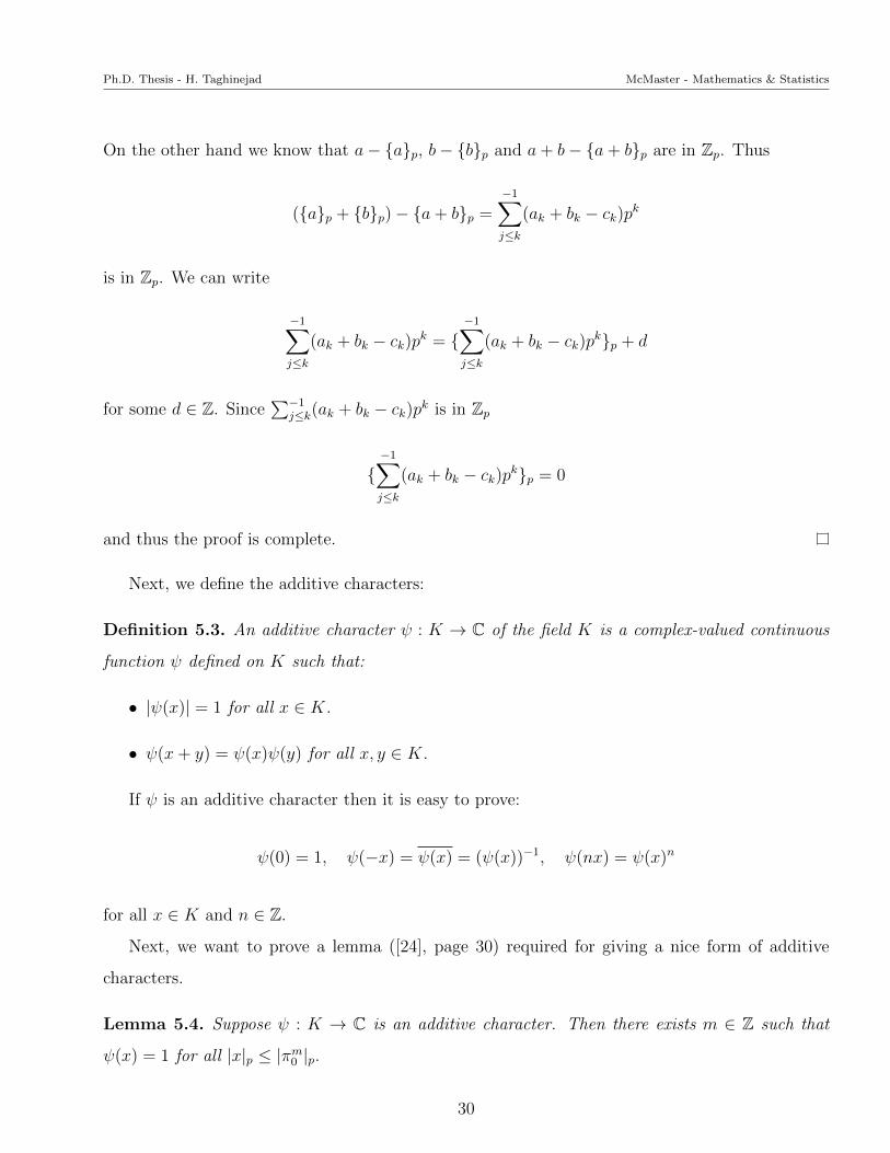
On the other hand we know that a− {a}p, b− {b}p and a+ b− {a+ b}p are in Zp. Thus
({a}p + {b}p)− {a+ b}p =−1∑j≤k
(ak + bk − ck)pk
is in Zp. We can write
−1∑j≤k
(ak + bk − ck)pk = {−1∑j≤k
(ak + bk − ck)pk}p + d
for some d ∈ Z. Since∑−1
j≤k(ak + bk − ck)pk is in Zp
{−1∑j≤k
(ak + bk − ck)pk}p = 0
and thus the proof is complete.
Next, we define the additive characters:
Definition 5.3. An additive character ψ : K → C of the field K is a complex-valued continuous
function ψ defined on K such that:
• |ψ(x)| = 1 for all x ∈ K.
• ψ(x+ y) = ψ(x)ψ(y) for all x, y ∈ K.
If ψ is an additive character then it is easy to prove:
ψ(0) = 1, ψ(−x) = ψ(x) = (ψ(x))−1, ψ(nx) = ψ(x)n
for all x ∈ K and n ∈ Z.
Next, we want to prove a lemma ([24], page 30) required for giving a nice form of additive
characters.
Lemma 5.4. Suppose ψ : K → C is an additive character. Then there exists m ∈ Z such that
ψ(x) = 1 for all |x|p ≤ |πm0 |p.
30
Ph.D. Thesis - H. Taghinejad McMaster - Mathematics & Statistics
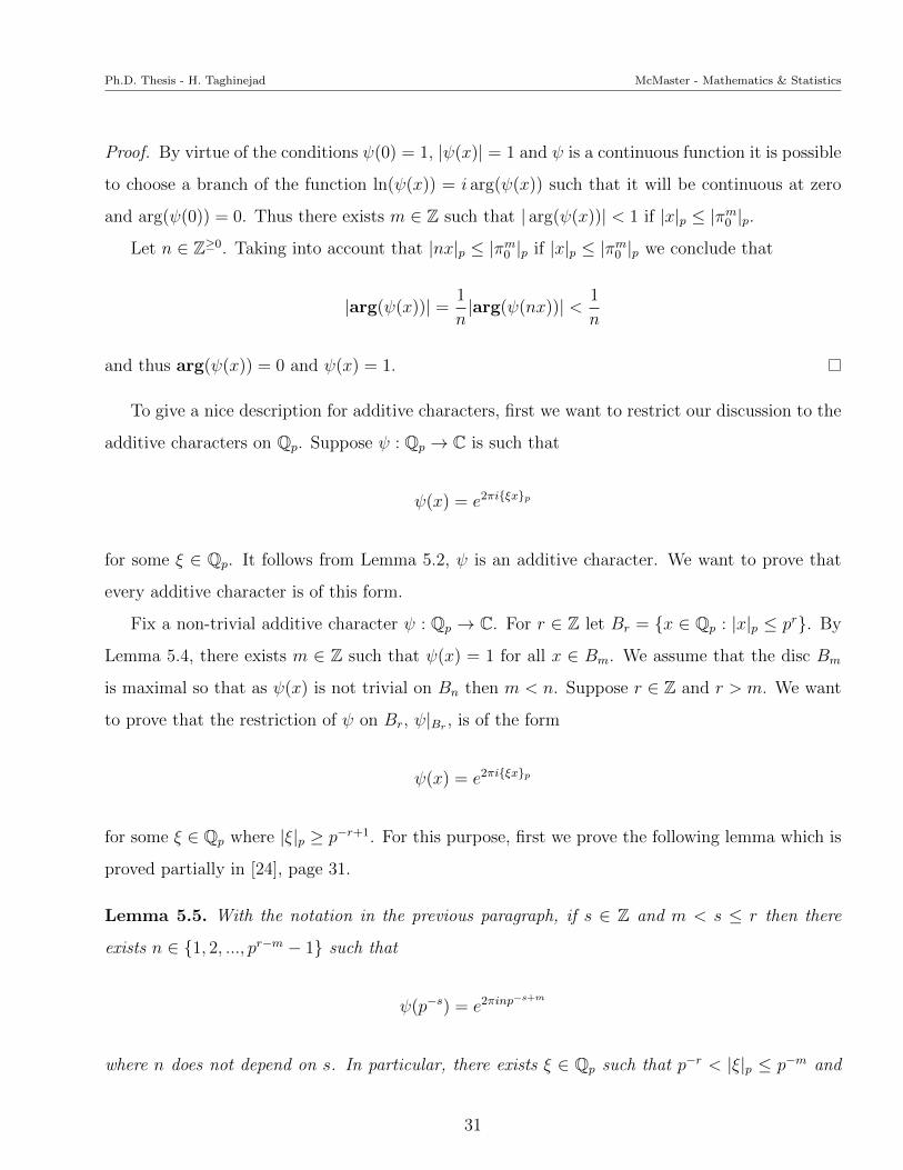
Proof. By virtue of the conditions ψ(0) = 1, |ψ(x)| = 1 and ψ is a continuous function it is possible
to choose a branch of the function ln(ψ(x)) = i arg(ψ(x)) such that it will be continuous at zero
and arg(ψ(0)) = 0. Thus there exists m ∈ Z such that | arg(ψ(x))| < 1 if |x|p ≤ |πm0 |p.
Let n ∈ Z≥0. Taking into account that |nx|p ≤ |πm0 |p if |x|p ≤ |πm0 |p we conclude that
|arg(ψ(x))| = 1
n|arg(ψ(nx))| < 1
n
and thus arg(ψ(x)) = 0 and ψ(x) = 1.
To give a nice description for additive characters, first we want to restrict our discussion to the
additive characters on Qp. Suppose ψ : Qp → C is such that
ψ(x) = e2πi{ξx}p
for some ξ ∈ Qp. It follows from Lemma 5.2, ψ is an additive character. We want to prove that
every additive character is of this form.
Fix a non-trivial additive character ψ : Qp → C. For r ∈ Z let Br = {x ∈ Qp : |x|p ≤ pr}. By
Lemma 5.4, there exists m ∈ Z such that ψ(x) = 1 for all x ∈ Bm. We assume that the disc Bm
is maximal so that as ψ(x) is not trivial on Bn then m < n. Suppose r ∈ Z and r > m. We want
to prove that the restriction of ψ on Br, ψ|Br , is of the form
ψ(x) = e2πi{ξx}p
for some ξ ∈ Qp where |ξ|p ≥ p−r+1. For this purpose, first we prove the following lemma which is
proved partially in [24], page 31.
Lemma 5.5. With the notation in the previous paragraph, if s ∈ Z and m < s ≤ r then there
exists n ∈ {1, 2, ..., pr−m − 1} such that
ψ(p−s) = e2πinp−s+m
where n does not depend on s. In particular, there exists ξ ∈ Qp such that p−r < |ξ|p ≤ p−m and
31
Ph.D. Thesis - H. Taghinejad McMaster - Mathematics & Statistics
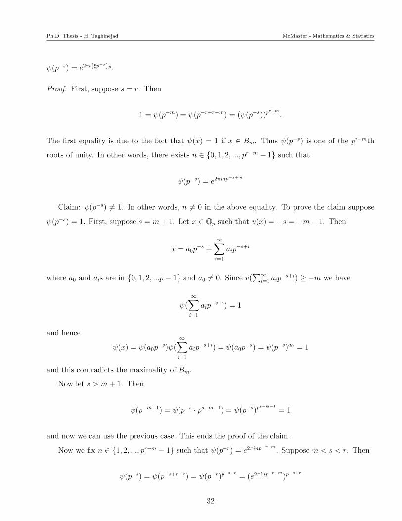
ψ(p−s) = e2πi{ξp−s}p.
Proof. First, suppose s = r. Then
1 = ψ(p−m) = ψ(p−r+r−m) = (ψ(p−s))pr−m
.
The first equality is due to the fact that ψ(x) = 1 if x ∈ Bm. Thus ψ(p−s) is one of the pr−mth
roots of unity. In other words, there exists n ∈ {0, 1, 2, ..., pr−m − 1} such that
ψ(p−s) = e2πinp−s+m
Claim: ψ(p−s) 6= 1. In other words, n 6= 0 in the above equality. To prove the claim suppose
ψ(p−s) = 1. First, suppose s = m+ 1. Let x ∈ Qp such that v(x) = −s = −m− 1. Then
x = a0p−s +
∞∑i=1
aip−s+i
where a0 and ais are in {0, 1, 2, ...p− 1} and a0 6= 0. Since v(∑∞
i=1 aip−s+i) ≥ −m we have
ψ(∞∑i=1
aip−s+i) = 1
and hence
ψ(x) = ψ(a0p−s)ψ(
∞∑i=1
aip−s+i) = ψ(a0p
−s) = ψ(p−s)a0 = 1
and this contradicts the maximality of Bm.
Now let s > m+ 1. Then
ψ(p−m−1) = ψ(p−s · ps−m−1) = ψ(p−s)ps−m−1
= 1
and now we can use the previous case. This ends the proof of the claim.
Now we fix n ∈ {1, 2, ..., pr−m − 1} such that ψ(p−r) = e2πinp−r+m
. Suppose m < s < r. Then
ψ(p−s) = ψ(p−s+r−r) = ψ(p−r)p−s+r
= (e2πinp−r+m
)p−s+r
32
Ph.D. Thesis - H. Taghinejad McMaster - Mathematics & Statistics
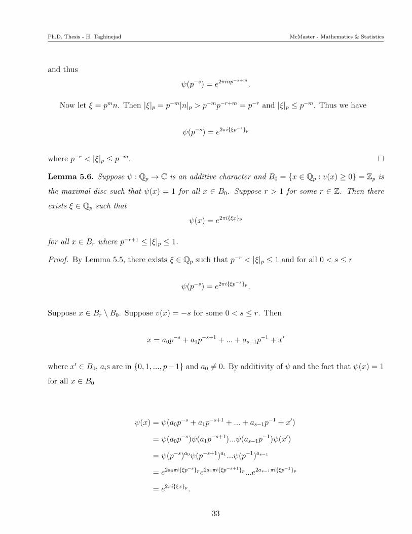
and thus
ψ(p−s) = e2πinp−s+m
.
Now let ξ = pmn. Then |ξ|p = p−m|n|p > p−mp−r+m = p−r and |ξ|p ≤ p−m. Thus we have
ψ(p−s) = e2πi{ξp−s}p
where p−r < |ξ|p ≤ p−m.
Lemma 5.6. Suppose ψ : Qp → C is an additive character and B0 = {x ∈ Qp : v(x) ≥ 0} = Zp is
the maximal disc such that ψ(x) = 1 for all x ∈ B0. Suppose r > 1 for some r ∈ Z. Then there
exists ξ ∈ Qp such that
ψ(x) = e2πi{ξx}p
for all x ∈ Br where p−r+1 ≤ |ξ|p ≤ 1.
Proof. By Lemma 5.5, there exists ξ ∈ Qp such that p−r < |ξ|p ≤ 1 and for all 0 < s ≤ r
ψ(p−s) = e2πi{ξp−s}p .
Suppose x ∈ Br \B0. Suppose v(x) = −s for some 0 < s ≤ r. Then
x = a0p−s + a1p
−s+1 + ...+ as−1p−1 + x′
where x′ ∈ B0, ais are in {0, 1, ..., p− 1} and a0 6= 0. By additivity of ψ and the fact that ψ(x) = 1
for all x ∈ B0
ψ(x) = ψ(a0p−s + a1p
−s+1 + ...+ as−1p−1 + x′)
= ψ(a0p−s)ψ(a1p
−s+1)...ψ(as−1p−1)ψ(x′)
= ψ(p−s)a0ψ(p−s+1)a1 ...ψ(p−1)as−1
= e2a0πi{ξp−s}pe2a1πi{ξp
−s+1}p ...e2as−1πi{ξp−1}p
= e2πi{ξx}p .
33
Ph.D. Thesis - H. Taghinejad McMaster - Mathematics & Statistics
Corollary 5.7. Suppose ψ : Qp → C is an additive character and Bm is the maximal disc such
that ψ(x) = 1 for all x ∈ Bm. Suppose r > m for some r ∈ Z. Then there exists ξ ∈ Qp such that
ψ(x) = e2πi{ξx}p
for all x ∈ Br where p−r+1 ≤ |ξ|p ≤ p−m.
Proof. Let χ(x) = ψ(p−mx). It is easy to check that χ(x) is an additive character on Qp and B0 is
the maximal disc such that χ(x) = 1 for all x ∈ B0. By the previous lemma, there exists ξ′ ∈ Qp
such that
χ(x) = e2πi{ξ′x}p
for all x ∈ pmBr where |ξ′|p ≥ p−r+m+1. Now let x ∈ Br. Then pmx ∈ pmBr and hence
ψ(x) = χ(pmx) = e2πi{ξ′pmx}p .
Let ξ = ξ′pm. Then
|ξ|p = |ξ′|pp−m ≥ p−r+1.
With the same method, we can conclude from |ξ′|p ≤ 1 that |ξ|p ≤ p−m.
Now we are ready to prove the main theorem of this chapter which is proved partially in [24],
page 32.
Theorem 5.8. Suppose ψ : Qp → C is an additive character. Then there exists ξ ∈ Qp such that
ψ(x) = e2πi{ξx}p
for all x .
Proof. Suppose Bm is the maximal disc such that ψ(x) = 1 for all x ∈ Bm. By Corollary 5.7, for
r = m+ 1, there exists ξ ∈ Qp such that
ψ(x) = e2πi{ξx}p
34
Ph.D. Thesis - H. Taghinejad McMaster - Mathematics & Statistics
for all x ∈ Bm+1 where v(ξ) = m. Let Sm+2 = {x ∈ Qp : v(x) = −m− 2}. Then Sm+2 ∩Bm+1 = ∅
and Bm+2 = Sm+2 ∪ Bm+1. First, suppose x ∈ Sm+2. There exists a0 ∈ {1, 2, ..., p − 1} and
x′ ∈ Bm+1 such that
x = a0p−m−2 + x′.
Then
ψ(x) = ψ(a0p−m−2)ψ(x′) = ψ(p−m−1)
a0p ψ(x′) = (e2πi{ξp
−m−1}p)a0p e2πi{ξx
′}p
= e2πi{a0ξp−m−2+ξx′}p = e2πi{ξ(a0p
−m−2+x′)}p = e2πi{ξx}p
Thus for all x ∈ Bm+2
ψ(x) = e2πi{ξx}p .
Continuing this process inductively, we can conclude
ψ(x) = e2πi{ξx}p
for all x ∈ Qp where v(ξ) = m.
Now let’s get back to the general case. Suppose ψ : K → C is an additive character where K
is a finite extension of Qp of degree n ∈ N. Then there are z1, ..., zn ∈ K such that for all x ∈ K,
x = a1z1 + ...+ anzn where a1, ..., an ∈ Qp. Thus
ψ(x) = ψ(a1z1 + ...+ anzn) = ψ(a1z1) · .... · ψ(anzn).
Fix i ∈ [n]. Let ψi : Qp → C be such that ψi(a) = ψ(azi). Then it is easy to check that ψi is an
additive character on Qp. Now by Theorem 5.8, there is ξi ∈ Qp such that
ψi(a) = e2πi{ξia}p
for all x ∈ Qp. Thus if x = a1z1 + ...+ anzn ∈ K then
ψ(x) = e2πi{ξ1a1}p · ... · e2πi{ξnan}p .
35
Ph.D. Thesis - H. Taghinejad McMaster - Mathematics & Statistics
Chapter 6
p-adic Van Der Corput’s Lemma
In this chapter, we state the p-adic Van Der Corput’s Lemma proved by Cluckers in [7] and
then we state and prove a modified version of this lemma which plays a key role in proving the
main theorem. The Van Der Corput’s Lemma is used by Stein in [23] to develope “the theory of
oscillatory integrals of the first kind”.
In [7], Cluckers proves a p-adic version of Van Der Corput’s Lemma in one and multidimensional
cases. In this chapter, first we give a generalized version of Cluckers’ theorem in Theorem 6.12
and then we use the result to prove Theorem 6.14 which is the the main goal of this chapter.
Through out this chapter, we fix K as a finite extension of Qp as we did in the previous chapters.
Rv is the valuation ring of K, Mv is the maximal ideal of Rv and q is the cardinality of the residue
field. Suppose x denotes one variable and let K{x} be the ring of restricted power series over K in
the variable x as we discussed in Chapter 2. Given f(x) =∑
i aixi ∈ K{x}, the supi{|ai|} exists.
Definition 6.1. Suppose f(x) =∑
i aixi is a restricted power series. We define the Gauss norm
of f , denoted by ||f ||, to be supi{|ai|}.
Among restricted power series, there are some power series, Special Power series (SP), which
can be approximated by their linear parts. The following definition is stated in [7] as Definition
2.2.
Definition 6.2. A power series∑
i aixi ∈ K{x} in one variable is called SP if a1 6= 0 and
aj ∈ a1Mv for all j > 1. If f ∈ K{x} is SP, we write |f |SP for |a1| which is equal to the Gauss
norm of f − f(0).
36
Ph.D. Thesis - H. Taghinejad McMaster - Mathematics & Statistics
To see why the SP power series can be approximated by their linear parts, Let c ∈ Rv and
f(x) =∑
i aixi ∈ K{x} be SP. Since f(c) − (a0 + a1c) is convergent, there is 1 < m ∈ N such
that amcm = supi>1{aici}. Since |c| ≤ 1, |amcm| ≤ |amc|. On the other hand, f is SP and thus
|am| < |a1|. Hence
|f(c)− (a0 + a1c)| ≤ |amcm| ≤ |amc| < |a1c| ≤ |f(c)|.
Since c ∈ Rv was arbitrary, for all x ∈ Rv we have
|f(x)− (a0 + a1x)| < |f(x)|.
Moreover, |f ′(x)| = |a1|.
The set of SP power series is a small subset of the restricted power series. We can convert some
non-SP restricted power series to an SP series by using some affine transformations. The following
definition is stated in [7] as Definition 2.3. For every integer r > 0, Let M rv = {dr|d ∈Mv} and let
M ′v = {d||d| = 1}.
Definition 6.3. Let f(x) ∈ K{x}. We define the SP-number of f to be the smallest integer r ≥ 0
such that for all nonzero c ∈M rv and all b ∈ Rv, the power series
fb,c(x) :=1
cf(b+ cx)
is SP if such r exists, and define the SP-number of f as ∞ otherwise.
With regard to the definition, f is SP if and only if the SP number of f is zero. To see that,
let f(x) =∑
i aixi ∈ K{x} and let bi be the ith coefficient of 1
c
∑ai(b + cx)i. It is easy to check
that
bi =∑m≥i
nmamci−1bm−i,
where nm ≥ 0 is an integer. Suppose f is SP and let c ∈ M ′v and b ∈ Rv. By the previous
discussion, b1 =∑
m≥1 nmambm−1. Since f is SP, |am| < |a1| for all m > 1 and hence |b1| = |a1|.
37
Ph.D. Thesis - H. Taghinejad McMaster - Mathematics & Statistics
For any i > 1,
|bi| ≤ maxm≥i{|nmamci−1bm−i|} < |a1| = |b1|.
Thus 1cf(b+cx) is SP. On the other hand if 1
cf(b+cx) is SP for all c ∈M ′
v and b ∈ Rv, in particular
it is SP when b = 0 and c = 1. In other words, f(x) is SP.
The next lemma is proved by Cluckers in [7]. In this lemma, we find a useful relation between
the Gauss norm, the SP-number and the cardinality of residue field.
Lemma 6.4. [7, Lemma 2.4] Let f(x) =∑
i aixi ∈ K{x} be such that |f ′(x)| ≥ 1 for all x ∈ Rv.
Then the SP-number of f is an integer r ≥ 0 satisfying
qr−1 ≤ ||f − f(0)||.
In addition, for all nonzero c ∈M rv and all b ∈ Rv, we have |fb,c|SP ≥ 1.
Proof. We refer the reader to Cluckers, [7], Lemma 2.4.
The following corollary extends the scope of Lemma 6.4.
Corollary 6.5. Let ε > 0 be an arbitrary real number and let f(x) =∑
i aixi ∈ K{x}. Suppose
that |f ′(x)| ≥ ε for all x ∈ Rv. Then the SP-number of f is an integer r ≥ 0 satisfying
qr−1 ≤ ||f − f(0)||ε
.
In addition, for all nonzero c ∈M rv and all b ∈ Rv, we have |fb,c|SP ≥ ε.
Proof. Let
ε′ = min{|x| : x ∈ K and |x| ≥ ε}
and let e ∈ K be such that |e| = ε′. By definition, |f ′(x)| ≥ |e| for all x ∈ Rv.
Let g(x) = f(x)e
. Then
|g′(x)| = |f′(x)
e| ≥ 1
for all x ∈ Rv. By the previous lemma, the SP-number of g is an integer r ≥ 0 satisfying
qr−1 ≤ ||g − g(0)||.
38
Ph.D. Thesis - H. Taghinejad McMaster - Mathematics & Statistics
Claim: The SP-numbers of g and f are the same.
Proof of claim: Suppose the SP-number of f is r and the SP-number of g is r′. Let c ∈ M rv and
b ∈ Rv. Since the SP-number of f is r, by Definition 6.3, fb,c(x) is SP. On the other hand
gb,c(x) =1
cg(b+ cx) =
1
cef(b+ cx) =
1
efb,c(x)
and thus gb,c is also SP. Thus r′ ≤ r. With the same argument we can prove r ≤ r′ and hence the
proof for the claim is complete.
By Definition 6.1,
||g − g(0)|| = ||f − f(0)|||e|
.
Thus the SP-number of f is an integer r ≥ 0 satisfying
qr−1 ≤ ||f − f(0)|||e|
=||f − f(0)||
ε′≤ ||f − f(0)||
ε.
By the previous lemma, for all nonzero c ∈M rv and all b ∈ R
|fb,c|SP|e|
= |gb,c|SP ≥ 1
and thus |fb,c|SP ≥ ε′ ≥ ε.
In the next step, we are going to prove another lemma that we use to prove Van Der Corput’s
lemma. Before stating the lemma, we need to go through some preparations.
Definition 6.6. Let f(x) ∈ Rv{x} be a power series whose coefficients come from the valuation
ring, Rv. We call f regular of degree d ≥ 0 if f(x) is congruent to a monic polynomial of degree
d modulo the maximal ideal Mv{x}.
Remark 6.7. If f =∑
i aixi ∈ K{x} is a restricted power series, Then, since |ai| → 0 as i→∞,
there are a unique d ≥ 0 and a unique c ∈ K× such that cf becomes regular of degree d. If f is
SP and |a0| ≤ |a1|, since a1 6= 0, we see that c is a−11 . Since |ai| < |a1| for all i > 1, f becomes
a0a−11 + x modulo the maximal ideal Mv{x}. Thus d = 1.
39
Ph.D. Thesis - H. Taghinejad McMaster - Mathematics & Statistics
The following is the statement of Weierstrass Preparation Theorem which can be found in [3]
or [1].
Theorem 6.8. Let f ∈ Rv{x} be regular of degree d. Then there are a unique monic polynomial
w ∈ R[x] of degree d and a unique unit u ∈ Rv{x} such that
f = w.u
Now we are ready to prove the following lemma that Cluckers uses to prove Van Der Corput’s
lemma. The lemma and the sketch of the proof can be found in [7]. We give a more detailed
version of the proof here.
Lemma 6.9. [13, Lemma 2.8] Let f(x) =∑
i aixi ∈ K{x}. Suppose that f is SP. If there exists
no d ∈ Rv such that f(d) = 0, then
|f(x)| = |a0| > |f |SP
for all x ∈ Rv. If there is d ∈ Rv such that f(d) = 0, then
|f(x)| = |f |SP .|x− d|.
In general, if e ∈ Rv is such that |f(e)| is minimal among the values |f(x)| for x ∈ Rv, then one
has for all x ∈ Rv
|f(x)| ≥ |f |SP |x− e|.
Proof. First we claim that |a0| ≤ |a1| = |f |SP if and only if there exists d ∈ Rv such that f(d) = 0.
Proof of claim: Suppsoe |a0| ≤ |a1|. Since f is a restricted power series and SP, by Remark 6.7,
we can convert f to a regular power series of degree one by multiplying its coefficients by a−11 . For
simplicity, let’s assume that |a1| = 1. By Weierstrass Preparation 6.8, there are a unique monic
polynomial w = b+ x ∈ Rv{x} of degree one and a unique unit u ∈ Rv{x} such that
f = w.u.
40
Ph.D. Thesis - H. Taghinejad McMaster - Mathematics & Statistics
Now let d = −b, then f(d) = 0 and d ∈ Rv. For the other direction, suppose that there is d ∈ Rv
such that f(d) = 0. Since f is SP,
|f(d)− (a0 + a1d)| ≤ |f(d)|
and thus a0 + a1d = 0. Hence |a0| ≤ |a1|.
If there exists no d ∈ Rv such that f(d) = 0, then |a0| > |a1| and since |aj| < |a1| for all j > 1,
|a0| > |aj| for all j ≥ 1. Thus for all x ∈ Rv
|f(x)| = |a0|
and this finishes the first case. Now suppose that there exists d ∈ Rv such that f(d) = 0. Let
g(t) = f(t+ d). Then g is SP and g(0) = 0. Let g(t) =∑
i≥1 biti. Then for t ∈ Rv
|g(t)| = |t||∑i≥1
biti−1|.
Since g is SP,
|g|SP = |b1| > |biti−1|
and thus
|g(t)| = |t|.|g|SP
and this finishes the second case.
For the final statement, any e ∈ Rv can serve in the first case and in the second case, we can
take e to be d.
An oscillatory integral is an integral of the form
∫Rv
f(x)ψ(y.φ(x))|dx|
where ψ is an additive character on K as introduced in Chapter 5 and |dx| is the normalized
Haar measure on K as introduced in Chapter 3. The function φ is usually called the phase and f
41
Ph.D. Thesis - H. Taghinejad McMaster - Mathematics & Statistics
the amplitude of the integral. For the many variables analogue, x or y can be tuples of variables
and φ can be a tuple of K-valued functions, and then y.φ is the standard inner product. By
using Theorem 5.8 and the paragraph after, we can assume that ψ is trivial on Mv and nontrivial
otherwise.
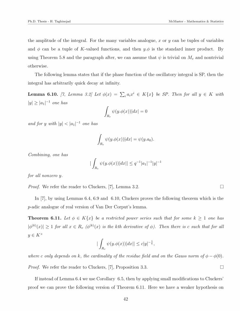
The following lemma states that if the phase function of the oscillatory integral is SP, then the
integral has arbitrarily quick decay at infinity.
Lemma 6.10. [7, Lemma 3.2] Let φ(x) =∑
i aixi ∈ K{x} be SP. Then for all y ∈ K with
|y| ≥ |a1|−1 one has ∫Rv
ψ(y.φ(x))|dx| = 0
and for y with |y| < |a1|−1 one has
∫Rv
ψ(y.φ(x))|dx| = ψ(y.a0).
Combining, one has
|∫Rv
ψ(y.φ(x))|dx|| ≤ q−1|a1|−1|y|−1
for all nonzero y.
Proof. We refer the reader to Cluckers, [7], Lemma 3.2.
In [7], by using Lemmas 6.4, 6.9 and 6.10, Cluckers proves the following theorem which is the
p-adic analogue of real version of Van Der Corput’s lemma.
Theorem 6.11. Let φ ∈ K{x} be a restricted power series such that for some k ≥ 1 one has
|φ(k)(x)| ≥ 1 for all x ∈ Rv (φ(k)(x) is the kth derivative of φ). Then there is c such that for all
y ∈ K×
|∫Rv
ψ(y.φ(x))|dx|| ≤ c|y|−1k ,
where c only depends on k, the cardinality of the residue field and on the Gauss norm of φ− φ(0).
Proof. We refer the reader to Cluckers, [7], Proposition 3.3.
If instead of Lemma 6.4 we use Corollary 6.5, then by applying small modifications to Cluckers’
proof we can prove the following version of Theorem 6.11. Here we have a weaker hypothesis on
42
Ph.D. Thesis - H. Taghinejad McMaster - Mathematics & Statistics
the derivative of the phase function and the constant c depends on M upper bound for the Gauss
norm of φ− φ(0).
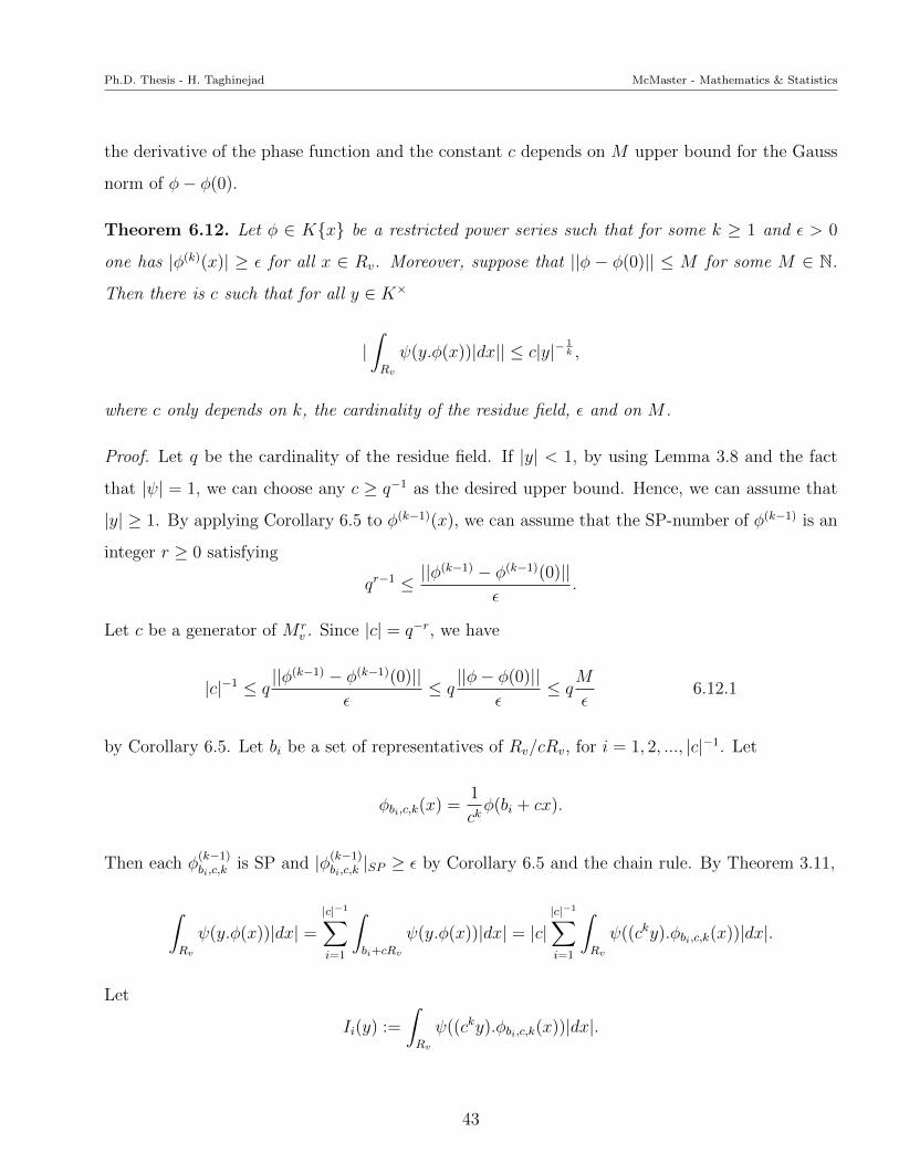
Theorem 6.12. Let φ ∈ K{x} be a restricted power series such that for some k ≥ 1 and ε > 0
one has |φ(k)(x)| ≥ ε for all x ∈ Rv. Moreover, suppose that ||φ − φ(0)|| ≤ M for some M ∈ N.
Then there is c such that for all y ∈ K×
|∫Rv
ψ(y.φ(x))|dx|| ≤ c|y|−1k ,
where c only depends on k, the cardinality of the residue field, ε and on M .
Proof. Let q be the cardinality of the residue field. If |y| < 1, by using Lemma 3.8 and the fact
that |ψ| = 1, we can choose any c ≥ q−1 as the desired upper bound. Hence, we can assume that
|y| ≥ 1. By applying Corollary 6.5 to φ(k−1)(x), we can assume that the SP-number of φ(k−1) is an
integer r ≥ 0 satisfying
qr−1 ≤ ||φ(k−1) − φ(k−1)(0)||
ε.
Let c be a generator of M rv . Since |c| = q−r, we have
|c|−1 ≤ q||φ(k−1) − φ(k−1)(0)||
ε≤ q||φ− φ(0)||
ε≤ q
M
ε6.12.1
by Corollary 6.5. Let bi be a set of representatives of Rv/cRv, for i = 1, 2, ..., |c|−1. Let
φbi,c,k(x) =1
ckφ(bi + cx).
Then each φ(k−1)bi,c,k
is SP and |φ(k−1)bi,c,k|SP ≥ ε by Corollary 6.5 and the chain rule. By Theorem 3.11,
∫Rv
ψ(y.φ(x))|dx| =|c|−1∑i=1
∫bi+cRv
ψ(y.φ(x))|dx| = |c||c|−1∑i=1
∫Rv
ψ((cky).φbi,c,k(x))|dx|.
Let
Ii(y) :=
∫Rv
ψ((cky).φbi,c,k(x))|dx|.
43
Ph.D. Thesis - H. Taghinejad McMaster - Mathematics & Statistics
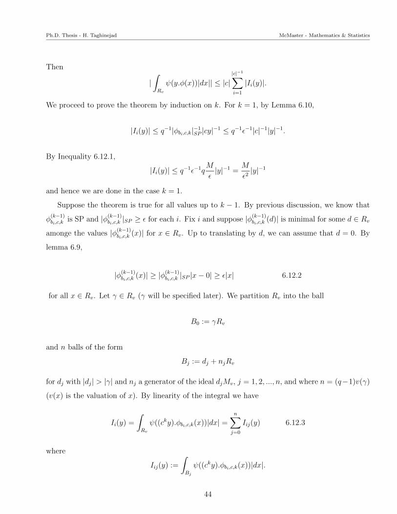
Then
|∫Rv
ψ(y.φ(x))|dx|| ≤ |c||c|−1∑i=1
|Ii(y)|.
We proceed to prove the theorem by induction on k. For k = 1, by Lemma 6.10,
|Ii(y)| ≤ q−1|φbi,c,k|−1SP |cy|−1 ≤ q−1ε−1|c|−1|y|−1.
By Inequality 6.12.1,
|Ii(y)| ≤ q−1ε−1qM
ε|y|−1 =
M
ε2|y|−1
and hence we are done in the case k = 1.
Suppose the theorem is true for all values up to k − 1. By previous discussion, we know that
φ(k−1)bi,c,k
is SP and |φ(k−1)bi,c,k|SP ≥ ε for each i. Fix i and suppose |φ(k−1)
bi,c,k(d)| is minimal for some d ∈ Rv
amonge the values |φ(k−1)bi,c,k
(x)| for x ∈ Rv. Up to translating by d, we can assume that d = 0. By
lemma 6.9,
|φ(k−1)bi,c,k
(x)| ≥ |φ(k−1)bi,c,k|SP |x− 0| ≥ ε|x| 6.12.2
for all x ∈ Rv. Let γ ∈ Rv (γ will be specified later). We partition Rv into the ball
B0 := γRv
and n balls of the form
Bj := dj + njRv
for dj with |dj| > |γ| and nj a generator of the ideal djMv, j = 1, 2, ..., n, and where n = (q−1)v(γ)
(v(x) is the valuation of x). By linearity of the integral we have
Ii(y) =
∫Rv
ψ((cky).φbi,c,k(x))|dx| =n∑j=0
Iij(y) 6.12.3
where
Iij(y) :=
∫Bj
ψ((cky).φbi,c,k(x))|dx|.
44
Ph.D. Thesis - H. Taghinejad McMaster - Mathematics & Statistics
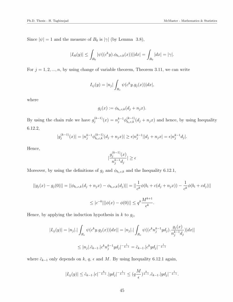
Since |ψ| = 1 and the measure of B0 is |γ| (by Lemma 3.8),
|Ii0(y)| ≤∫B0
|ψ((cky).φbi,c,k(x))||dx| =∫B0
|dx| = |γ|.
For j = 1, 2, ..., n, by using change of variable theorem, Theorem 3.11, we can write
Iij(y) = |nj|∫Rv
ψ(cky.gj(x))|dx|,
where
gj(x) := φbi,c,k(dj + njx).
By using the chain rule we have g(k−1)j (x) = nk−1j φ
(k−1)bi,c,k
(dj + njx) and hence, by using Inequality
6.12.2,
|g(k−1)j (x)| = |nk−1j φ(k−1)bi,c,k
(dj + njx)| ≥ ε|nk−1j ||dj + njx| = ε|nk−1j dj|.
Hence,
|g(k−1)j (x)
nk−1j dj| ≥ ε
Moreover, by using the definitions of gj and φbi,c,k and the Inequality 6.12.1,
||gj(x)− gj(0)|| = ||φbi,c,k(dj + njx)− φbi,c,k(dj)|| = ||1
ckφ(bi + c(dj + njx))− 1
ckφ(bi + cdj)||
≤ |c−k|||φ(x)− φ(0)|| ≤ qkMk+1
εk.
Hence, by applying the induction hypothesis in k to gj,
|Iij(y)| = |nj|.|∫Rv
ψ(cky.gj(x))|dx|| = |nj|.|∫Rv
ψ((cknk−1j ydj).gj(x)
nk−1j dj)|dx||
≤ |nj|.ck−1.|cknk−1j ydj|−1
k−1 = ck−1.|ckydj|−1
k−1
where ck−1 only depends on k, q, ε and M . By using Inequality 6.12.1 again,
|Iij(y)| ≤ ck−1.|c|−kk−1 .|ydj|−
1k−1 ≤ (q
M
ε)
kk−1 .ck−1.|ydj|−
1k−1 .
45
Ph.D. Thesis - H. Taghinejad McMaster - Mathematics & Statistics
Let
c′k−1 = (qM
ε)
kk−1 .ck−1.
Therefore, we have
|Iij(y)| ≤ c′k−1|ydj|− 1k−1
where c′k−1 only depends on k, q, ε and M . Now by using 6.12.3,
|Ii(y)| ≤ |γ|+n∑j=1
|Iij(y)| ≤ |γ|+ c′k−1|y|− 1k−1
n∑i=1
|dj|−1
k−1 .
By the definition of dj, 0 ≤ v(dj) ≤ v(γ). For each l with 0 ≤ l ≤ v(γ), there are q − 1 different
dj with v(dj) = l. Thus
n∑i=1
|dj|−1
k−1 = (q − 1)
v(γ)−1∑l≥0
(q1/(k−1))l = (q − 1)|γ|−1/(k−1) − 1
q1/(k−1) − 1
≤ |γ|−1/(k−1) q − 1
q1/(k−1) − 1.
Therefore,
|Ii(y)| ≤ |γ|+ c′′k−1|γy|− 1k−1
where c′′k−1 only depends on k, q, ε and M . Since |y| ≥ 1, if we can choose γ ∈ Rv such that
q−1|y|−1k ≤ |γ| < |y|−
1k ,
then
|Ii(y)| ≤ c′′′k |y|−1k
where c′′′k only depends on k, q, ε and M . By using the definition of Ii, we can find the desired
bound for I and the proof is complete.
Remark 6.13. Let {φi}i∈I ⊆ K{x} be a an arbitrary set of restricted power series such that for
some k ≥ 1 one has |φ(k)i (x)| ≥ ε for all x ∈ Rv and for all i ∈ I. Moreover, suppose that for
46
Ph.D. Thesis - H. Taghinejad McMaster - Mathematics & Statistics
all i ∈ I, ||φi − φi(0)|| ≤ M for some M ∈ N .Then, since according to the previous theorem, c
only depends on k, the cardinality of residue field, ε and on M , there is a single c such that for all
y ∈ K× and all i ∈ I
|∫Rv
ψ(y.φi(x))|dx|| ≤ c|y|−1k ,
where c only depends on k, the cardinality of residue field, ε and on M .
The version of Van Der Corput’s lemma stated in the previous two theorems applies when the
domain of integration is the valuation ring Rv. To prove the main theorem, we need a more flexible
version of these theorems. To be more precise, we need a modified version of Van Der Corput’s
lemma in which the domain of integration is any subanalytic set of the form {x ∈ K| |a| ≤ |x| ≤
|b|, x ∈ λPn}.
Theorem 6.14. Let
E = {x ∈ K| |a| ≤ |x| ≤ |b|, x ∈ λPn}
where λ ∈ K×, a, b ∈ K and n ∈ N. Let φ(x) =∑∞
i=0 aixi be a power series which is convergent
on E and suppose that for some k ≥ 1, |φ(k)(x)| ≥ ε for all x ∈ E. Then there is c such that
|∫E
ψ(y.φ(x))|dx|| ≤ c|y|−1k
for all y ∈ K×.
Proof. First we want to prove that without loss of generality we can assume that λ = 1. Let
ξ : K → K be the analytic function defined by ξ(x) = λx. Let
E ′ = {x ∈ K| |aλ−1| ≤ |x| ≤ |bλ−1|, x ∈ Pn}.
Then ξ is an analytic isomorphism from E ′ onto E. By Theorem 3.11, we have
∫E
ψ(y.φ(x))|dx| = λ
∫E′ψ(y.φ(ξ(x)))|dx|.
It is obvious that φ(ξ(x)) is a convergent power series on E ′ and |(φ ◦ ξ)(k)(x))| ≥ ε|λ|k. Thus, the
47
Ph.D. Thesis - H. Taghinejad McMaster - Mathematics & Statistics
hypotheses of the theorem apply to φ ◦ ξ and it suffices to prove the theorem where
E = {x ∈ K| |a| ≤ |x| ≤ |b|, x ∈ Pn}.
Let
V alE = {i ∈ Z| |a| ≤ (1
p)i ≤ |b|, n|i}.
Let An = {e1, e2, ..., em} be a set of representatives in K for those elements of the residue field
which have an nth root. For i ∈ V alE and j ∈ [m], Let
Eij = {x ∈ K| x = ejπi0 + d for some |d| ≤ (
1
p)i+1},
where π0 is the uniformizer of K (|π0| = 1p). By using Theorem 2.2 and Lemma 2.9, It is easy to
see that E = ∪i,jEij and thus
∫E
ψ(y.φ(x))|dx| =∑i,j
∫Eij
ψ(y.φ(x))|dx|.
For i ∈ V alE and j ∈ [m] let ξij : K → K be such that ξij(x) = πi+10 x+ ejπ
i0. Then
ξij(Rv) = Eij
and ξij defines an analytic isomorphism from Rv onto Eij. By Theorem 3.11, we have
|∫Eij
ψ(y.φ(x))|dx|| = |πi+10 |.|
∫Rv
ψ(y.φ(ξij(x))|dx||.
φ ◦ ξij(x) is a convergent power series on Rv and it is easy to see that
|(φ ◦ ξij)(k)(x)| ≥ ε|π0|k(i+1)
and hence|(φ ◦ ξij)(k)(x)||π0|k(i+1)
≥ ε.
48
Ph.D. Thesis - H. Taghinejad McMaster - Mathematics & Statistics
The coefficients of φ ◦ ξij are the summation of the terms of form akπt(i+1)0 (ejπ
i0)k−t for t ∈
{0, 1, 2, 3, ..., k}. Since |ej| = 1 and by the definition of V alE, we can easily check that |πi+10 | ≤
|b|p
and |πi0| ≤ |b|. Thus for k 6= 0
|akπt(i+1)0 (ejπ
i0)k−t| ≤ |ak|
|b|k
pt≤ |ak||b|k ≤ sup
i{|ai||b|i}.
Since φ(b) is finite, the right side of above inequality is finite. Hence ||φ◦ξij−φ◦ξij(0)|| is bounded
above by supi{|ai||b|i} for all i and j.
Now by Remark 6.13, there is c′ such that
∫Rv
ψ(y.φ(ξij(x))|dx| =∫Rv
ψ(πk(i+1)0 y.
φ(ξij(x))
πk(i+1)0
)|dx| ≤ c′|πk(i+1)0 y|−
1k = c′
|y|− 1k
|π(i+1)0 |
for all y ∈ K× and all i and j. Thus
|∫E
ψ(y.φ(x))|dx|| ≤∑i,j
|∫Eij
ψ(y.φ(x))|dx|| =∑i,j
|π0|i+1|∫Rv
ψ(y.φ(ξij(x))|dx||
≤∑i,j
c′|y|−1k = nc′|y|−
1k .
in which n is the total number of indexes we have. Let c = nc′ and the proof is complete.
49
Ph.D. Thesis - H. Taghinejad McMaster - Mathematics & Statistics
Chapter 7
Main Theorem
In this chapter, we prove the main theorem of this thesis by using Van Der Corput’s lemma and
its corollary which is proved in previous chapter as Theorem 6.14. First we restate the theorem.
Theorem 7.1. Let φ : Rmv → K be an analytic map satisfying the hyperplane condition. Let
f ∈ C(Rmv ) be integrable and suppose ψ is an additive character. Let ε > 0. Then there are real
numbers s < 0 and c > 0 such that
|∫Rmv
f(x)ψ(y.φ(x))|dx|| ≤ cmin{1, |y|s}+ ε
for all y ∈ K×. Moreover, s does not depend on ε while c does.
To prove the theorem we need to go through some preparation. The following lemma plays
an important role in the proof of main theorem. The notation of this lemma comes from chapter
four, Theorem 4.10.
Lemma 7.2. Suppose A ⊆ Rmv is a cell over ∅ and let g > 0 be an integer. Let
H(x) = t.(m∏j=1
|(xj − cj(x1, ..., xj−1))ajuajj |
1nj )(
m∏j=1
v(xj − cj(x1, ..., xj−1))sj)
be a constructible function where t = |w| or t = v(w) for some w ∈ K and sj ≥ 0 and aj are
50
Ph.D. Thesis - H. Taghinejad McMaster - Mathematics & Statistics
integers. Assume H is a positive valued map on A. Moreover, let E ⊆ (K \Rv) ∪ {0} × A be
E = {(λ, x) | |λ|−r ≤ |(xj − cj(x1, ..., xj−1))| ≤ |λ|r, for all j ∈ {1, ...,m}}.
Then, if we take r > 0 to be small enough, there is a constant c > 0 such that
H(x) ≤ c|λ|g
for all λ ∈ (K \Rv) ∪ {0} and x ∈ Eλ.
Proof. Let I ⊆ [m] be such that aj ≥ 0 for all j ∈ I. Then
|(xj − cj(x1, ..., xj−1))| ≤ |λ|r =⇒ |(xj − cj(x1, ..., xj−1))|ajnj ≤ |λ|
rajnj
for all j ∈ I. On the other hand, if j ∈ [m] \ I,
|λ|−r ≤ |(xj − cj(x1, ..., xj−1))| =⇒ |(xj − cj(x1, ..., xj−1))|ajnj ≤ |λ|
−rajnj
For j ∈ [m] let bj =rajnj
if j ∈ I and bj =−rajnj
if j ∈ [m] \ I. Then
|(xj − cj(x1, ..., xj−1))|ajnj ≤ |λ|bj
for all j ∈ [m]. To find an appropriate upper bound for v(xj − cj(x1, ..., xj−1))sj first we notice
that v(x) = − logp |x|. Let J ⊆ [m] such that for j ∈ J , v(xj − cj(x1, ..., xj−1)) ≥ 0. Then
|λ|−r ≤ |(xj − cj(x1, ..., xj−1))| =⇒ logp(|λ|−r) ≤ logp(|(xj − cj(x1, ..., xj−1))|)
=⇒ − logp(|(xj − cj(x1, ..., xj−1))|) ≤ − logp(|λ|−r) =⇒ v(xj − cj(x1, ..., xj−1)) ≤ r logp(|λ|)
=⇒ v(xj − cj(x1, ..., xj−1))sj ≤ (r logp(|λ|))sj
for all j ∈ J . On the other hand, if j ∈ [m] \ J
|(xj − cj(x1, ..., xj−1))| ≤ |λ|r =⇒ logp(|(xj − cj(x1, ..., xj−1))|) ≤ logp(|λ|r)
51
Ph.D. Thesis - H. Taghinejad McMaster - Mathematics & Statistics
=⇒ − logp(|(xj − cj(x1, ..., xj−1))|) ≥ − logp(|λ|r) =⇒ v(xj − cj(x1, ..., xj−1)) ≥ −r logp(|λ|)
=⇒ −v(xj − cj(x1, ..., xj−1)) ≤ r logp(|λ|) =⇒ (−1)sjv(xj − cj(x1, ..., xj−1))sj ≤ (r logp(|λ|))sj .
Let J1 ⊆ [m] \ J such that sj is an even positive integer for all j ∈ J1 and let J2 ⊆ [m] \ J such
that sj is an odd positive integer for all j ∈ J2. For j ∈ J1
v(xj − cj(x1, ..., xj−1))sj ≤ (r logp(|λ|))sj .
Without loss of generality we can assume t ≥ 0. Since H(x) is a positive valued function, the
cardinality of J2, must be an even number and thus∑
j∈J2 sj is an even number. Hence
∏j∈J2
v(xj − cj(x1, ..., xj−1))sj =∏j∈J2
(−1)sjv(xj − cj(x1, ..., xj−1))sj ≤∏j∈J2
(r logp(|λ|))sj
By considering the above inequalities we can conclude
H(x) = (t∏j∈[m]
|uj|ajnj )(
∏j∈[m]
|(xj − cj(x1, ..., xj−1))|)ajnj (
∏j∈[m]
v(xj − cj(x1, ..., xj−1))sj)
≤ (t∏j∈[m]
|uj|ajnj )(
∏j∈[m]
|λ|bj)(∏j∈[m]
(r logp(|λ|))sj)
= (t∏j∈[m]
rsj |uj|ajnj ).|λ|
∑j∈[m] bj .(logp(|λ|))
∑j∈[m] sj .
If we take r to be small enough such that∑
j∈[m] bj ≤g2, then since |λ| > 1 we have
|λ|∑j∈[m] bj ≤ |λ|
g2 .
On the other hand if we take r to be small enough and c > 0 to be large enough then
(t∏j∈[m]
rsj |uj|ajnj )(logp(|λ|))
∑j∈[m] sj ≤ c|λ|
g2 .
52
Ph.D. Thesis - H. Taghinejad McMaster - Mathematics & Statistics
By combining the last two equalities, we have
H(x) ≤ c|λ|g.
The following lemma gives us a powerful tool to find the decay rate of constructible functions.
In [8], Cluckers and Miller prove a similar lemma in the real case. For stating and proving the
lemma, we need the following definition.
Definition 7.3. Suppose {Eλ}λ∈K is a family of subsets of a set A ⊆ Km. Let B ⊆ A. We say
Eλ → B as |λ| → ∞ if Eλ ⊆ Eλ′ whenever |λ| < |λ′| and
B =⋃λ∈K
Eλ.
If Eλ → B′ where B′ \B has measure 0, we say Eλ → B almost everywhere and we write Eλ → B
a.e.
Lemma 7.4. Let f ∈ C(U) for a subanalytic set U ⊂ Km. Let f be integrable and E ⊂ K ×U be
a subanalytic set such that Eλ → ∅ a.e. as |λ| → ∞ where Eλ = {x ∈ U : (λ, x) ∈ E} for λ ∈ K.
Then there is α < 0 such that ∫Eλ
f(x)|dx| � min{1, |λ|α}
for all λ ∈ K.
Proof. By using Theorem 4.9, we can decompose U into cells A such that f |A is a finite sum∑ni=1Hi(x), where each Hi is a constructible function on A of the form given in Theorem 4.9.
Moreover, by Theorem 4.9, we can choose A such that each Hi is integrable with a constant sign
on A. It suffices to focus on f |A. Moreover, since
|∫Eλ∩A
f(x)|dx|| ≤∫Eλ∩A
|f(x)||dx| ≤∑i
∫Eλ∩A
|Hi(x)||dx|
and |Hi(x)| is a constructible function on A, it suffices to focus on the case where the integrand is
53
Ph.D. Thesis - H. Taghinejad McMaster - Mathematics & Statistics
|Hi| for some i. For suppose that for every i there are ci and αi < 0 such that
∫Eλ∩A
|Hi(x)||dx| ≤ cimin{1, |λ|αi}.
Let c = max{ci} and α = max{αi}. By using the properties of reciprocal functions, we
know that for any λ ∈ K either |λ|αi ≥ 1 for all i or |λ|αi < 1 for all i. In the first case, since
min{1, |λ|αi} = 1 for all i, we have min{1, |λ|α} = 1 and
|∫Eλ∩A
f(x)|dx|| ≤ n.c.min{1, |λ|α}
in which n is the number of indices. In the second case, since |λ|αi ≤ |λ|α we have the desired
property with the same upper bound as in the above inequality.
To prove the lemma for |Hi(x)|, first we notice that |Hi(x)| is a constructible function since Hi
does not change its sign. Let χ : K×Km → R be the characteristic function of Eλ∩A. Obviously,
|χ| is a constructible function and
∫Eλ∩A
|Hi(x)||dx| ≤∫A
|Hi(x)|.|χ(λ, x)||dx|.
Let G(λ) :=∫A|Hi(x)|.|χ(λ, x)||dx|. Then by Theorem 4.5, G(λ) is a constructible function.
Moreover, when |λ| → ∞, Eλ → ∅ and so G(λ) → 0. Now by Corollary 4.8, there is αi < 0 such
that
G(λ)� min{1, |λ|αi}
and hence the proof is complete.
In the main theorem, the phase function, φ(x), is an analytic map satisfying the hyperplane
condition. We refer the reader to chapter one, Definition 1.2, for the definition of the hyperplane
condition. To be able to use Van Der Corput’s lemma to prove the theorem, we need to convert
the hyperplane condition to a condition on partial derivatives of the phase function. That is the
purpose of the following lemma. If x = (x1, x2, ..., xm) and i = (i1, i2, ..., im) ∈ Nm, then we write
xi to mean xi11 xi22 ...x
imm . We write |i| which is defined to be
∑mj=1 ij.
54
Ph.D. Thesis - H. Taghinejad McMaster - Mathematics & Statistics
Lemma 7.5. Let φ(x) =∑
i∈Nm aixi be a restricted power series satisfying the hyperplane condition
where x = (x1, x2, ..., xm). Then there are a number n ∈ N, b1, ..., bn ∈ Rmv , r1, ..., rn ∈ {pi|i ∈ Z},
ε1, ..., εn ∈ R and k1, ..., kn ∈ Nm with |ki| > 0 such that for each i ∈ [n]
|∂kix φ(x)| > εi
if |x− bi| ≤ ri, where ∂kix φ = (∏
j∂kij
∂xkijj
)φ. Moreover, we can choose the bi and the ri such that
Rmv ⊆
⋃i∈[n]
{x| |x− bi| ≤ ri}
Proof. Let b ∈ Rmv . Consider the function φ(x)−φ(b) mapping Rm
v into K. This function does not
vanish identically on a neighborhood of b. For suppose Vb is an open set containing b such that
φ(x)− φ(b) = 0
for all x ∈ Vb. Then Vb ⊆ φ−1({φ(b)}). However {φ(b)} ⊆ K is a hyperplane and hence
µ(φ−1({φ(b)})) = 0 by the hyperplane condition. That is a contradiction since µ(Vb) > 0.
We can write
φ(x) =∑i∈Nm
aixi =
∑i∈Nm
ai[(x− b) + b]i =∑i∈Nm
ci(x− b)i
in which ci = ∂ixφ(b). If ∂ixφ(b) = 0 for all i with |i| > 0, φ(x) − φ(b) would vanish identically
on Rmv which is not possible by previous argument. Thus there is k ∈ Nm with |k| > 0 such that
∂kxφ(b) 6= 0. Let ε > 0 be such that |∂kxφ(b)| > ε. Since |∂kxφ(x)| is continuous, there is r ∈ R such
that
|∂kxφ(x)| > ε
if |x− b| ≤ r. Thus for every b ∈ Rmv there are r, ε and k satisfying the above inequality with the
given condition. Since Rmv is compact, there are b1, ..., bn ∈ Rm
v , r1, ..., rn ∈ {pi|i ∈ Z}, ε1, ..., εn ∈ R
and k1, ..., kn ∈ Nm with |ki| > 0 such that
|∂kix φ(x)| > εi
55
Ph.D. Thesis - H. Taghinejad McMaster - Mathematics & Statistics
if |x− bi| ≤ ri for all i ∈ [n] and
Rmv ⊆ ∪i∈[n]{x| |x− bi| ≤ ri}.
Let x = (x1, x2, ..., xm) and let Vk,m(K) be the K-vector space of homogeneous polynomials
of degree k in x over K. In [7], Cluckers proves the following lemma that we are going to use to
obtain a nicer description of partial derivatives of the phase function.
Lemma 7.6. [7, Lemma 3.7] Let α > 0 be an integer and x = (x1, ..., xm) variables. Let K be an
infinite field of characteristic > α or zero. Then the polynomials of the form
(ξ.x)α
for ξ ∈ Kn, where ξ.x =∑
i ξixi, span the K-vector space Vα,m(K) of homogeneous polynomials of
degree α in x over K.
Proof. We refer the reader to Cluckers, [7]. Note that we can take ξ of length one.
Now we are ready to prove the main theorem.
Proof of Theorem 7.1. Let x = (x1, ..., xm). Since φ is analytic, it can be written as a convergent
power series locally on Rmv . By compactness of Rm
v , for some n ∈ N, there are b1, ..., bn ∈ Rmv and
r1, ..., rn ∈ {pi|i ∈ Z} such that for each j ∈ [n], there are {aij}i∈Nm such that
φ(x) =∑i∈Nm
aji(x− bj)i on |x− bj| ≤ rj
and {x||x− bj| ≤ rj}j forms an open cover for Rmv .
For j ∈ [n] let
gj : Rmv → {x||x− bj| ≤ rj},
gj(x) = rjx+ bj.
56
Ph.D. Thesis - H. Taghinejad McMaster - Mathematics & Statistics
Then gj is an analytic isomorphism such that
φ(gj(x)) =∑i∈Nm
aji[(rjx+ bj)− bj]i =∑i∈Nm
ajirijxi,
which is a convergent power series on Rmv . Moreover, φ(gj(x)) satisfies the hyperplane condition
since the image of a set of measure zero under an affine transformation has measure zero. By
Theorem 3.11
|∫Rmv
f(x)ψ(y.φ(x))|dx|| ≤ |∑j∈[n]
∫{x||x−bj |≤rj}
f(x)ψ(y.φ(x))|dx|| (7.1)
≤∑j∈[n]
|rj||∫Rmv
f(gj(x))ψ(y.φ(gj(x)))|dx||. (7.2)
It is enough to prove the theorem for each integral in the above inequality. Thus, without loss of
generality we can assume φ(x) =∑
i aixi is a restricted power series on Rv.
Since φ(x) is a restricted power series satisfying the hyperplane condition, Lemma 7.5 implies
that there are b1, ..., bn ∈ Rmv , r1, ..., rn ∈ {pi|i ∈ Z}, ε1, ..., εn ∈ R and k1, ..., kn ∈ Nm with |ki| > 0
such that for each i ∈ [n]
|∂kix φ(x)| ≥ εi
if |x− bi| ≤ ri, where |ki| =∑
j kij and ∂kix φ = (∏
j∂kij
∂xkijj
)φ. Moreover, {x| |x− bi| ≤ ri} forms an
open cover for Rmv . Thus, by using ”change of variable theorem” and the same argument that we
used before, we can assume that φ(x) is a restricted power series such that there is k ∈ Nm with
|k| > 0 and there is ε ∈ R so that we have
|∂kxφ(x)| > ε
for all x ∈ Rmv .
Let α = |k| =∑
j kj. By Lemma 7.6, there are ξ1, ..., ξd ∈ Km of length 1 such that the
homogeneous polynomials
(ξi.x)α i = 1, 2, ..., d
57
Ph.D. Thesis - H. Taghinejad McMaster - Mathematics & Statistics
form a basis for this vector space, where d is the dimension of Vα,m(K) as a K-vector scpace.
Express the monomial xk in this basis as
xk =∑i
ei(ξi.x)α, ei ∈ K.
Let
∂Vα,m(K) = {∑
d1+d2+...+dm=α
ed1,...,dm∂(d1,...,dm)x φ | ed1,...,dm ∈ K, d1, ..., dm ≥ 0},
where ∂(d1,...,dm)x φ = (
∏i∂di
∂xdij
)φ. Obviously, ∂Vα,m(K) is a vector space over K. Define
σ : Vα,m(K) −→ ∂Vα,m(K),
σ(∑
d1+d2+...+dm=α
ed1,...,dmxd11 ...x
dmm ) =
∑d1+d2+...+dm=α
ed1,...,dm∂d1,...,dmx φ.
Then σ defines an isomorphism from Vα,m(K) onto ∂Vα,m(K) such that
σ((ξi.x)α) = (ξi.∇)αφ,
where ∇ = ( ∂∂x1, ∂∂x2, ..., ∂
∂xm). Then, for b ∈ Rm
v ,
ε < |∂kxφ(b)| = |∑i
ei(ξi.∇)αφ(b)| ≤ maxi{|ei(ξi.∇)αφ(b)|}.
Hence
|(ξi.∇)αφ(b)| > ε
ei
for at least one i with ei 6= 0. Since |(ξi.∇)αφ(x)| is a continuous function there is r ∈ {pi|i ∈ Z}
such that
|(ξi.∇)αφ(x)| > ε
ei
if |x − b| ≤ r. Hence by using a measure preserving affine transformation and change of variable
58
Ph.D. Thesis - H. Taghinejad McMaster - Mathematics & Statistics
theorem, as the first argument in the proof, we can assume
|(∂α/∂xα1 )φ(x)| > ε
for all x ∈ Rmv and some ε ∈ R≥0.
By Theorem 4.10, we can partition Rmv into cells A over ∅ such that f |A is a finite summation
of the functions of the form
H(x) = t.(m∏j=1
|(xj − cj(x1, ..., xj−1))ajuajj |
1nj )(
m∏j=1
v(xj − cj(x1, ..., xj−1))sj)
where t = |w| or t = v(w) for some w ∈ K and sj ≥ 0 and aj are integers. We can choose
the partitions such that H(x) is integrable on A and does not change its sign. Without loss of
generality, we can assume that H(x) is positive on A. It is enough to prove the theorem for H(x)
over A. Moreover, if π1(A) is the projection of A on the first coordinate, then
π1(A) = {t ∈ K||a|�1|t− c1| ≤ |b|, t− c1 ∈ λPn}
with constants n > 0,λ, c1 ∈ K, a, b ∈ K×, and �1 either < or no condition. By using the affine
transformation g : Km → Km with g(x1, ..., xm) = (x1 + c1, ..., xm) and by using the change of
variable theorem we can assume c1 is zero.
Let E ⊆ {(K \Rv) ∪ {0}} × A be:
E = {(λ, x) | |λ|−r ≤ |(xj − cj(x1, ..., xj−1))| ≤ τ, for all j ∈ {1, ...,m}}
where τ = b when j = 1 and τ = |λ|r otherwise. Here r is a positive rational number, to be
specified later. The idea of defining E in this way helps us to separate the finite and infinite parts
of A. A \ Eλ → ∅ a.e when |λ| → ∞. By Lemma 7.4, there is γ < 0 and c1 > 0 such that:
∫A\Eλ
|H(x)||dx| ≤ c1 min{1, |λ|γ}
59
Ph.D. Thesis - H. Taghinejad McMaster - Mathematics & Statistics
and since
|∫A\Eλ
H(x)ψ(y.φ(x))|dx|| ≤∫A\Eλ
|H(x)||dx|
we can conclude ∫A\Eλ
H(x)ψ(y.φ(x))|dx| � min{1, |λ|γ}.
Thus it suffices to find a suitable bound for
|∫Eλ
H(x)ψ(y.φ(x))|dx||.
Let 0 < g < 1α
and let r > 0 to be large enough such that Lemma 7.2 holds. Then by Lemma 7.2,
there is c2 > 0 such that H(x) ≤ c2|λ|g for all λ ∈ (K \Rv) ∪ {0} and x ∈ Eλ. Thus
|∫Eλ
H(x)ψ(y.φ(x))|dx|| ≤ c2|λ|g.|∫Eλ
ψ(y.φ(x))|dx||
and hence it is enough to find an appropriate upper bound for
|∫Eλ
ψ(y.φ(x))|dx||.
Let π1(A) be the projection of A on the first coordinate and π2:m(A) be the projection of A on the
last m− 1 coordinate. By Fubini’s theorem we have
|∫Eλ
ψ(y.φ(x))|dx|| = |∫π2:m(Eλ)
∫π1(Eλ)
ψ(y.φ(x))|dx1||dx2...dxm||.
For each a2, ..., am ∈ Rv, the Gauss norm of φ(x1, a2, ..., , am) − φ(0, a2, ..., am) is bounded by
||φ(x)− φ(0)||. Hence by Theorem 6.14, there is c3 such that
|∫π1(Eλ)
ψ(y.φ(x1, a2, ..., am))|dx1|| ≤ c3|y|−1α
for all a2, ..., am ∈ Rv,y ∈ K× and λ. Thus
|∫Eλ
ψ(y.φ(x))|dx|| ≤ |∫π2:m(Eλ)
c3|y|−1α |dx2...dxm|| ≤ c3|y|−
1α
60
Ph.D. Thesis - H. Taghinejad McMaster - Mathematics & Statistics
in which the last inequality is the result of µ(π2:m(Eλ)) ≤ 1 (since π2:m(Eλ) ⊆ Rm−1). Hence
|∫Eλ
H(x)ψ(y.φ(x))|dx|| ≤ c3c2|λ|g|y|−1α .
Let |λ| be large enough such that
c1|λ|γ ≤ ε.
Now let c = max{∫A|H(x)||dx|, 1, c2c3|λ|g}. Let y ∈ K×. If |y| ≤ 1, then 1 ≤ |y|− 1
α and
|∫A
H(x)ψ(y.φ(x))|dx|| ≤∫A
|H(x)||dx| ≤ c = cmin{1, |y|−1α}.
If |y| > 1, then
|∫A\Eλ
H(x)ψ(y.φ(x))|dx|| ≤ c1|λ|γ
and
|∫Eλ
H(x)ψ(y.φ(x))|dx|| ≤ c2c3|λ|g|y|−1α
and thus
|∫A
H(x)ψ(y.φ(x))|dx|| ≤ c2c3|λ|g|y|−1α + c1|λ|γ ≤ c2c3|λ|g|y|−
1α + ε ≤ c|y|−
1α + ε.
Hence
|∫A
H(x)ψ(y.φ(x))|dx|| � min{1, |y|−1α}+ ε.
Let s = − 1α
and the proof is complete.
The last statement in the theorem is the result of applying Theorem 6.14 in which the exponent
only depends on the partial derivative of the phase function.
As an interesting topic for future research in this area, one can think about finding a method to
eliminate ε dependency in the main theorem. As another topic, one can think about the possibility
of proving the main theorem in the case φ is defined on K instead of Rv.
61
Ph.D. Thesis - H. Taghinejad McMaster - Mathematics & Statistics
Bibliography
[1] M. Aschenbrenner, An effective Weierstrass Division Theorem, unpublished preprint avail-
able at http://www.math.ucla.edu/ matthias/publications.html.
[2] S. Albeverio, A. Yu. Khrennikov, V. M. Shelkovich, Theory of p-adic distributions,
Linear and non linear models, London Mathematical Society, Lecture Note Series 370.
[3] S. Bosch, U. Guntzer, and R. Remmert, Non-Archimedean Analysis. A systematic
approach to rigid analytic geometry, Grundlehren Math. Wiss., vol. 261, Springer-Verlag,
Berlin, 1984.
[4] R. Cluckers, p-adic semialgebraic sets and cell decomposition, Journal fur die reine und
angewandte Mathematik 369 (1986), 154–166.
[5] R. Cluckers, Multivariate Igusa theory: decay rates of exponential sums, Int. Math. Res.
Not. 76 (2004), 4093–4108.
[6] R. Cluckers, Analytic p-adic cell decomposition and integrals, Trans. Amer. Math. Soc. 356
(2004), no. 4, 1489–1499.
[7] R. Cluckers, Analytic Van Der Corput Lemma for p-Adic and Fq((t)) Oscillatory Integrals,
Singular Fourier Transforms, and Restriction Theorems, Expos. Math. 29(4), 371–386 (2011).
[8] R. Cluckers, Daniel J. Miller, Bounding the decay of oscillatory integrals with a con-
structible amplitude function and a globally subanalytic phase function, Journal of Fourier
Analysis and Applications, Volume 22, Issue 1, 215–236, 2016
62
Ph.D. Thesis - H. Taghinejad McMaster - Mathematics & Statistics
[9] J. Denef, The rationality of the Poincare series associated to the p-adic points on a variety,
Inventiones Mathematicae 77 (1984).
[10] J. Denef, L. van den Dries, p-adic and real subanalytic sets, Annals of Mathematics 128
(1988), no. 1, 79–138.
[11] L. van den Dries, Tame topology and o-minimal structures, Lecture Note Series, vol. 248,
Cambridge University Press, (1998).
[12] A. J. Engler, A. Prestel, Valued fields, Springer,(2000).
[13] V.P.Havin, N.K.Nikolski, Commutative Harmonic Analysis II, Encyclopedia of Mathe-
matical Sciences, volume 25, Springer.
[14] J. Igusa, Lectures on forms of higher degree (notes by S. Raghavan), Lectures on mathematics
and physics, Tata institute of fundamental research, vol. 59, Springer-Verlag, (1978).
[15] K. Iwasawa, Local Class Field Theory , Oxford University Press (New York),(1986).
[16] N. Leopoldo, The Haar integral, D. Van Nostrand Co. Inc. Princeton, N.J.Toronto-London,
MR 0175995, (1965).
[17] B. Lichtin, On a question of Igusa: towards a theory of several variable asymptotic
expansions II, https://www.cambridge.org/core/journals/compositio-mathematica/article/on-
a-question-of-igusa-ii-uniform-asymptotic-bounds-for-fourier-transforms-in-several-
variables/01EDF307B228AEF36126F6197B1E5E50.
[18] J. M. Lion, J. P. Rolin, Integration of subanalytic functions and volumes of subanalytic
subspaces, Ann. Inst. Fourier 48 (1998), no. 3, 755–767.
[19] A. Macintyre, On definable subsets of p-adic fields, J.symb.logic 41(1976), 605-610.
[20] M. Popa, Lecture notes on p-adic and motivic integration, chapter 3,
http://www.math.northwestern.edu/ mpopa/571/chapter6.pdf.
[21] D. Ramakrishnan, R. J. Valenza, Fourier analysis on number fields, Springer, (1999).
63
Ph.D. Thesis - H. Taghinejad McMaster - Mathematics & Statistics
[22] E. T. Sawyer, Lecture notes in advanced real analysis,
http://ms.mcmaster.ca/sawyer/Publications/AdvancedRealAnalysis.pdf (2010).
[23] E. M. Stein, Harmonic analysis: real-variable methods, orthogonality, and oscillatory in-
tegrals, Princeton Mathematical Series, vol. 43, Princeton University Press, Princeton, NJ,
(1993), With the assistance of Timothy S. Murphy, Monographs in Harmonic Analysis, III.
[24] V. S. Vladimirov, I. V. Volovich, E. I. Zelenov, p-adic Analysis and Mathematical
Physics, Woild Scientific Publishing Co. Pte. Lid, (1994).
[25] B. L. van der Waerden, Algebra, I, II, Springer-Verlag, New York, Heidelberg, Berlin,
(1964).
64

![-ADIC ELLIPTIC POLYLOGARITHM, -ADIC EISENSTEIN SERIES … · 2018-10-24 · arXiv:0707.3747v1 [math.NT] 25 Jul 2007 p-ADIC ELLIPTIC POLYLOGARITHM, p-ADIC EISENSTEIN SERIES AND KATZ](https://img.pdfslide.net/doc/110x75/5e26cc60ef471f7d09533bad/adic-elliptic-polylogarithm-adic-eisenstein-series-2018-10-24-arxiv07073747v1.jpg)