Bounds on double-diffusive convection - Mathematics, Department of

J. Fluid Mech. (2006), vol. 569, pp. 29–50. c© 2006 Cambridge University Press

doi:10.1017/S0022112006002230 Printed in the United Kingdom

29

Bounds on double-diffusive convection

By NEIL J. BALMFORTH,1,2 SHILPA A. GHADGE,1

ATICHART KETTAPUN 3 AND SHREYAS D. MANDRE 1

1Department of Mathematics, University of British Columbia, Vancouver,BC, V6T 1Z2, Canada

2Department of Earth and Ocean Sciences, University of British Columbia,Vancouver, BC, V6T 1Z2, Canada

3Department of Mathematics, University of California, Santa Cruz, CA 95064, USA

(Received 5 June 2005 and in revised form 3 May 2006)

We consider double-diffusive convection between two parallel plates and computebounds on the flux of the unstably stratified species using the background method.The bound on the heat flux for Rayleigh–Benard convection also serves as a boundon the double-diffusive problem (with the thermal Rayleigh number equal to thatof the unstably stratified component). In order to incorporate a dependence of thebound on the stably stratified component, an additional constraint must be included,like that used by Joseph (Stability of Fluid Motion, 1976, Springer) to improve theenergy stability analysis of this system. Our bound extends Joseph’s result beyond hisenergy stability boundary. At large Rayleigh number, the bound is found to behavelike R

1/2T for fixed ratio RS/RT , where RT and RS are the Rayleigh numbers of the

unstably and stably stratified components, respectively.

1. IntroductionMathematical models describing physical flows often have multiple possible solu-

tions that prove difficult to find due to the complex nature of the basic equations.Worse still, such flows are often turbulent, which precludes computing some of thephysically relevant solutions owing to the inability to resolve the finest scales. Inthis situation, it is helpful to search for other, more indirect approaches to theproblem that may assist in understanding crucial characteristics of the flow. One suchapproach is upper bound theory, wherein one avoids the search for actual solutions,but places bounds on some of their average properties. Malkus (1954) was the first topropose this kind of idea in the context of thermal convection (the Rayleigh–Benardproblem), and Howard (1963) subsequently set the theory on a firm mathematicalbasis and devised techniques to calculate the bound. Whilst the governing partialdifferential equations (PDEs) themselves are abandoned, the method retains twointegrals relations, or ‘power integrals’, derived from them, which is the crux of howthe approach is far simpler than direct computations.

Making use of clever inequalities, Howard deduced rigorous but rough bounds onthe heat flux that scaled like R

1/2T , where RT is the Rayleigh number. Howard also

computed bounds using test functions with a single horizontal wavenumber, whichleads to the alternative scaling, R

3/8T , for large RT . The single-wavenumber bound is

only valid if other functions do not lead to a higher value of the heat flux, whichBusse (1969) later showed to be the case at sufficiently high Rayleigh number. He alsogeneralized Howard’s approach using an elaborate procedure to account for more thanone wavenumber, and recovered the R

1/2T scaling in the infinite Rayleigh number limit.

30 N. J. Balmforth, S. A. Ghadge, A. Kettapun and S. D. Mandre

Howard’s method centres on a decomposition of all the physical fields intohorizontal averages and fluctuations about them. In an alternative approach, theConstantin–Doering–Hopf (CDH) background method (Doering & Constantin 1996),the variables are also decomposed, but this time exploiting arbitrary ‘background’fields. Integral identities similar to the ones used in Howard’s method are constructed,and the choice for the background is dictated by constraints similar to those obtainedin energy stability theory (see Joseph 1976). Work by Nicodemus, Grossmann &Holthaus (1997) and Kerswell (1998) has proved that, although the Howard–Busseand the CDH methods appear different, they are complementary or optimal duals ofeach other, and ultimately lead to the same result.

In this article, we use the background method to place bounds on double-diffusiveconvection (i.e. convection resulting from the dependence of buoyancy on twoproperties that diffuse at different rates). Such systems are often termed thermohaline,referring to their most common occurrence in oceans and other large water bodies,with salt and heat playing the roles of the two components. Interesting dynamicsensues when the two components affect the density stratification in opposite senses,and convection may occur even when the total density gradient is gravitationally stable(Veronis 1965; Baines & Gill 1969). For example, near the polar ice caps, meltingof ice releases fresh but cold water near the surface, a situation prone to oscillatorydouble-diffusive (ODD) convection (Jacobs et al. 1981; Neal, Neshira & Denner1969). ODD convection is also thought to occur in meddies (vortices of warm, saltywater commonly observed in the East Atlantic emanating from the Mediterranean,Ruddick (1992)). In an astrophysical context, ODD convection is believed to operatein the interiors of older stars where the two components are entropy and the elementsproduced by thermonuclear reactions (Spiegel 1969); mixing by ODD convection mayreplenish the reactive core of the star with fresh fuel and thus affect its evolution.

The opposite case, in which salt stratification is destabilizing but heat is stabilizing,is susceptible to the formation of salt fingers. Stern (1969) proposed that enhancedfluxes resulting from these fingers are instrumental in forming the staircase-likesalinity profiles observed in laboratory experiments and the open ocean. The articles byMerryfield (2000) and Schmitt (1994) provide recent reviews on this subject. Analoguesof salt fingers have also been suggested to arise in some astrophysical situations,where the role of salt is played by locally overabundant heavier elements such ashelium (Ulrich 1972; Vauclair 2004). In all these applications quantifying the degreeof mixing generated by thermohaline processes is paramount, which highlights theimportance of characterizing the flux laws in double-diffusive convection, especiallyin the turbulent regime. Whilst the desired characterization of the flux laws remainselusive to analysis, at least at present, we follow Malkus’s vision and calculate anupper bound on the flux of the unstably stratified species.

For double diffusion, this bounding exercise has two key novelties compared tothe Rayleigh–Benard problem. First, at the onset of convection, double-diffusivesystems show a richer array of dynamics than purely thermal systems. In Rayleigh–Benard convection, when the system first becomes convectively unstable, a branchof steady convection solutions bifurcates supercritically from the motionless state;that is, there is a smooth onset to steady overturning. This simple scenario does notcarry over to the double-diffusive case: as one raises RT to drive the system intoconvection, the linear instability can take the form of either steady overturning oroscillatory convection. Furthermore, the steady bifurcation can become subcritical,which implies the existence of multiple finite-amplitude solutions at lower Rayleighnumber that must, in turn, appear in saddle-node bifurcations at yet lower RT .

Bounds on double-diffusive convection 31

The existence of multiple solutions demands that the conductive state be subjectto finite-amplitude instability, even if it is linearly stable. All such dynamics mustbecome embedded in the upper bound, which may even jump discontinuously at thesaddle-node bifurcations. This raises the interesting question of whether the upperbound theory can be used to detect and characterize finite-amplitude instability andsaddle-node bifurcations.

Second, the bounding exercise also has some interesting mathematical twists. Wefirst show that the upper bound obtained on the flux of the unstably stratified com-ponent in the absence of the other component also serves as a bound in the presenceof that stabilizing field. In fact, this is the result that appears when we extend thebackground method in a straightforward way to doubly-diffusive convection. Whilstthis result is heuristically expected, since the stratification of the stable componentcan only diminish the flux, it fails to provide a dependence on both components.In previous attempts, Lindberg (1971) and Straus (1973) used variants of the single-wavenumber approach to bound the ODD and salt-fingering cases, respectively. Inorder to obtain a non-trivial dependence of the bound on the salt flux, Lindbergmaximized the heat and salt fluxes simultaneously. Not only is there no reason toexpect a single wavenumber, there is also no justification for assuming the fluxesto be maximal simultaneously. The procedure yielded bounds that scaled like R

3/8T ,

where RT now denotes the Rayleigh number of the unstably stratified component.Straus exploited the large difference between the diffusivities of heat and salt to solvethe heat equation asymptotically, thereby building the full effects of the stabilizingcomponent into the bounding formulation automatically. But like Lindberg’s, Straus’sbound also scales with the 3/8 power of RT , and again reflects the inadequacy ofa single wavenumber. In the current work, we identify one more integral constrainton double-diffusive convection, which Joseph (1976) has shown to be crucial inenergy stability analysis. By augmenting the upper bound analysis with this integralconstraint, and avoiding the use of a single wavenumber, we capture the effect ofboth components and construct a true bound. A similar analysis was also presentedby Stern (1982).

2. Mathematical formulationAs is traditionally done, we model our system by the Boussinesq equations:

ut+ u · ∇u = −∇p

ρ+ g(αT T − αSS) z+ ν∇2u, (2.1)

Tt+ u · ∇T = κT ∇2T , (2.2)

St+ u · ∇S = κS∇2S, (2.3)

∇ · u = 0, (2.4)

where u(x, t) is an incompressible velocity field, and T and S represent two scalarcomponents that affect the density of the fluid. We only deal with the situation inwhich the two components affect the density stratification in opposite senses; withoutloss of generality, we set T to be unstably stratified and S to be stably stratified. Ifthe diffusivity of T (κT ) is larger than that of S (κS) the system is susceptible to ODDconvection. In the opposite case, the system is susceptible to ‘T -fingers’ (because inthis case T is playing the role of salt). The other physical parameters are theacceleration due to gravity (g), coefficients of expansion due to variations in S (αS)and T (αT ), and the kinematic viscosity (ν).


We prescribe the values of S and T at the two boundaries, z = 0 and z = H :

T (z = H ) = Ttop, T (z = 0) = Ttop+ �T, (2.5)

S(z = H ) = Stop, S(z = 0) = Stop+ �S. (2.6)

For the velocity field, we either use the no-slip condition,

u = 0, (2.7)

or stress-free conditions,

w = 0, uz = vz = 0. (2.8)

Both these cases are considered when calculating the bound. However, the linearstability and some nonlinear solutions that we present are computed using the stress-free conditions, mostly for computational convenience.

We place the equations in dimensionless form by rescaling,

u → κT

Hu, T − Ttop → �T T, S − Stop → �S S, x → H x,

t → H 2

κT

t, p − ρg(αT Ttop − αSStop)z → ρκ2T

H 2p.

⎫⎪⎬⎪⎭ (2.9)

This gives rise to four dimensionless numbers,

RT =gαT �T H 3

νκT

, RS =gαS�SH 3

νκS

, Pr =ν

κT

, β =κS

κT

, (2.10)

and the governing equations become

1

Pr(ut+ u · ∇u + ∇p) = (RT T − βRSS) z + ∇2u, (2.11)

Tt + u · ∇T = ∇2T , (2.12)

St + u · ∇S = β∇2S, (2.13)

∇ · u = 0. (2.14)

The accompanying boundary conditions are

T (z = 1) = S(z = 1) = 0,

T (z = 0) = S(z = 0) = 1,

}(2.15)

plus (2.7) or (2.8) on z = 0 and z = 1 and periodicity in x and y.

3. Energy stabilityWe start with the criteria for nonlinear stability of the purely conductive state of this

system. A very brief account of this analysis was given by Joseph (1976). We elaborateand build upon Joseph’s results here in order to offer a more complete discussionand extract some important physical results; in doing so, we also emphasize the keyconnection with the bounding theory to follow.

3.1. Mathematical details

Consider u = 0 + u(x, t), T = T0 + θ(x, t), S = S0 + σ (x, t), and p = P0 + Π , whereT0 = S0 = 1 − z and P0 =Pr(RT − βRS)(z − z2/2) characterize the purely conductivesolution of (2.11)–(2.14), and u, θ , σ and Π are arbitrary perturbations. The


perturbations satisfy

1

Pr(ut + u · ∇u + ∇Π) = (RT θ − βRSσ ) z + ∇2u, (3.1)

θt + u · ∇θ − w = ∇2θ, (3.2)

σt + u · ∇σ − w = β∇2σ, (3.3)

∇ · u = 0. (3.4)

The kinetic energy equation is constructed by taking the dot product of the momentumequation (3.1) with u and integrating over the domain,

1

2Pr〈|u|2〉t = −〈|∇u|2〉 + RT 〈θw〉 − βRS〈σw〉, (3.5)

where

〈· · ·〉 ≡ 1

4LxLy

∫ Ly

−Ly

∫ Lx

−Lx

∫ 1

0

· · · dz dx dy,

2Lx and 2Ly are the periodicities in x and y, respectively, and |∇u|2 = ∇u: ∇uT .Similarly, by multiplying (3.2) and (3.3) by θ and σ , respectively, and integrating, wearrive at the following power integrals:

12〈θ2〉t = −〈|∇θ |2〉+ 〈θw〉, (3.6)

12〈σ 2〉t = −β〈|∇σ |2〉+ 〈σw〉. (3.7)

While these integral equations are the obvious generalization of those used for theenergy stability for thermal convection, there is a less obvious integral which is alsocrucial. It is constructed by multiplying (3.2) by σ and adding it to the product of(3.3) and θ and integrating:

〈θσ 〉t = 〈(θ + σ )w〉 − (1 + β)〈∇θ · ∇σ 〉. (3.8)

The optimal way in which to combine these integral equations so as to yield the beststability criterion is the essence of the analysis. Since we do not know the optimalcombination a priori, we start with an arbitrary linear combination of (3.5)–(3.8) andarrive at the generalized energy equation:

Et = −〈|∇u|2〉 − λ2T RT 〈|∇θ |2〉 − βλ2

SRS〈|∇σ |2〉 + λT RT bT 〈θw〉

+

√βλSRSbS

α〈σw〉 − (1 + β)cλT λS

√RT RS〈∇θ · ∇σ 〉, (3.9)

where

α2 = RS/RT , (3.10)

E ≡ 1

2Pr〈|u|2〉 +

λ2T RT

2〈θ2〉 +

λ2SRS

2〈σ 2〉 + cλT λS

√RT RS〈θσ 〉, (3.11)

bT ≡ 1

λT

+ λT + cαλS, (3.12)

bS ≡ −√

βα

λS

+α√βλS+

c√βλT , (3.13)

and λT , λS and c are the constants used to form the combination. When RS = 0 theeffect of S disappears and we recover the result for thermal convection. The basicstate is said to be ‘energy stable’ when the energy-norm, E, of the perturbations is


positive definite and decays monotonically (the right-hand side of (3.9) is negativedefinite) for all possible perturbations. It is straightforward to show that E in (3.11)is positive definite when |c| < 1.

First, we demonstrate the inability of (3.5)–(3.7) to capture the stabilizing effect ofRS when c =0. In this case, the energy equation takes the form,

Et = RT

(1 + λ2

T

)〈θw〉 + α2RT

(−β + λ2

S

)〈σw〉

− RT

(λ2

T 〈|∇θ |2〉 +α2βλ2S〈|∇σ |2〉

)− 〈|∇u|2〉 (3.14)

and we refer to E as the ‘regular’ energy. The optimization problem of finding thecritical RT leads to the criterion for stability,

RT < RT c =4Rc

F (λT , λS), (3.15)

where Rc is the critical Rayleigh number for the onset of thermal convection and

F (λT , λS) =

(1

λT

+ λT

)2

+

(− β

λS

+ λS

)2

. (3.16)

The choice of boundary conditions on the velocity enters the consideration throughthe value of Rc. For no slip, Rc ≈ 1707, whereas for the stress-free condition Rc ≈ 657.We now choose λT and λS to maximize the range of RT for which perturbations decay.That is, we look for the minimum value of the function F (λT , λS), which occurs forλ2

S =β and λT = 1, giving RT c = Rc, as stated earlier. To improve this stability conditionwe must take c = 0, thereby including (3.8).

Going back to (3.9), the terms involving ∇θ and ∇σ are negative semi-definite onlyif c � 2

√β/(1 + β). We choose c =2

√β/(1 + β) and then combine all three terms

into 〈|∇f |2〉, where

f ≡ λT

√RT θ + λS

√βRSσ.

This leaves us with just two sign-indefinite terms, 〈θw〉 and 〈σw〉. This pair canonly be bounded if they can again be grouped together in the combination f , whichprompts the constraint

bT = bS. (3.17)

The energy equation now takes the form

Et = R1/2T bT 〈f w〉 − 〈|∇f |2〉 − 〈|∇u|2〉, (3.18)

which is very similar to the one obtained for thermal convection, but with a modifiedthermal Rayleigh number and the field f playing the role of temperature. Againfinding the optimal perturbation, we conclude that the condition for energy stabilityis

RT < RT c =4Rc

b2T

. (3.19)

We still have the freedom to choose one of either λT or λS so as to obtain the bestpossible stability criterion. This leads to the following minimization problem for thecritical thermal Rayleigh number (RT c):

RT c = 4Rc

(minbT =bS

bT (λT , λS)2

)−1

. (3.20)


The details of the minimization are given in the Appendix. The resulting stabilitycondition can be encapsulated in the formulae

RT c =

⎧⎨⎩

Rc + RS if α � β < 1 or β � 1 > α

(√

Rc(1 − β2) + β√

RS)2 if β <α < β−1

∞ if α � β−1 > 1 or α � 1 and β � 1,

(3.21)

which were derived previously by Joseph.

3.2. Interpretation for stress-free plates

Now we draw some conclusions from Joseph’s result and compare with linear stabilitytheory, specifically for the case of stress-free plates. The linear stability theory isdescribed by Veronis (1965) and can be summarized as follows: linear instability canappear as either steady or oscillatory convection, the corresponding critical Rayleighnumbers being given by

steady: RT = RS + Rc, if α2 β +Pr

1 + Pr< β < 1 or β > 1, (3.22)

oscillatory: RT = (Pr + β)

(βRS

1 + Pr+

Rc(1 + β)

Pr

)if α2 β + Pr

1 + Pr> β and β < 1.

(3.23)

In figure 1, the energy stability condition (3.21) is compared with the conditions forthe onset of linear and nonlinear instability. First consider the fingering case (β > 1),represented in figure 1(a), which is the same for all values of β and Pr. In this case,the conductive state becomes linearly unstable to steady convection on the line (3.22),and is never unstable to oscillatory convection. The energy stability threshold agreeswith linear onset everywhere, proving that all perturbations, irrespective of their size,should decay below that line.

The ODD case (β < 1) is rather more complicated, and the dynamics of the systemdepends on the detailed parameter settings. Figures 1(b) and 1(c) show a repre-sentative case with β = 0.5 and Pr= 2; once we fix those parameters, the behaviourof the system is determined by where it falls on the (RS/Rc, RT /Rc)-plane, andthe range of possibilities is delimited by the four curves shown in the figure. Forα <

√β(1 + Pr)/(β + Pr) (left of point B), steady convection appears on the line

(3.22) and is the only linear instability. For α <β , or to the left of point A, the energystability condition in (3.21) also agrees with steady onset. However, to the right of thatpoint, the two conditions diverge from one another, indicating that energy stabilityis lost before the motionless state becomes linearly unstable to steady convection.The steady instability is further superceded by the onset of oscillatory convection forα >

√β(1 + Pr)/(β + Pr), or to the right of point B in figure 1(c). Moreover, except

at one special point (labelled D) where the two curves are tangential, energy stabilitynever agrees with linear oscillatory instability. In other words, only over a limitedparameter range does the loss of energy stability correspond to the onset of linearinstability, in contrast to thermal convection and the fingering case, where they alwaysagree.

Part of the reason for the disagreement between the energy stability conditionand linear onset arises because the steady bifurcation becomes subcritical at pointA. To the right of this point, the subcritical instability leads to steady convectionsolutions even in the linearly stable regime. These steady convection solutions do notpersist very far below the steady linear stability line because they turn around at asaddle-node bifurcation (Veronis 1965). The saddle node in the past has been located


0

2

4

6

8

10

(a)

(c)

(b)

102 4 6 8 12 14 0 102 4 6 8 12 14

Rc

RT

unstable

Stable

Line

ar a

nd g

ener

aliz

ed e

nerg

yRegular energy

2

4

6

8

10

Unstable

Stable

Stea

dy

Saddle-

node Oscill.

Generalized energy

Regular energy

1

2

3

4

5

6

8 106420

A

B

C

D

Unstable

Steady

Saddle-nodeOscill.

Generalized energyRc

RT

RT /Rc

RS /Rc RS /Rc

Figure 1. Stability boundaries on the (RS/Rc-RT /Rc)-plane. (a) The fingering case (β > 1),where the only linear instability is that of steady convection and the generalized energystability condition agrees with it (topmost curve). The curve below it shows the regular energystability criterion. These curves do not depend on the precise values of β and Pr. (b) TheODD case (β = 0.5 and Pr = 2) and to clarify the details a magnified view is plotted in (c).The topmost solid line corresponds to the onset of steady convection which is supercriticalto the left of point A and subcritical to its right. The unstable branch bifurcating from thesubcritical bifurcation turns around at a saddle–node bifurcation whose location is shown bythe dashed-dotted line. The nonlinear solutions at the saddle-node are calculated by expandingthe variables in a truncated Fourier series in x and a sine series in z. The dashed line showsthe linear stability criterion for onset of oscillatory convection. The solid lines again show thegeneralized and regular energy stability conditions, respectively.

using a crude Galerkin truncation of the governing equations. To improve upon this,we have accurately computed the locus of that bifurcation numerically via Fourierexpansion and a continuation algorithm. The locus is plotted in figure 1. In the regionbetween this locus and the onset of steady convection, multiple steady solutions areguaranteed.

When multiple solutions exist, certain finite-amplitude perturbations and the energyassociated with them will not decay to zero but saturate to a finite value, reflectinga transition to one of the other solutions. As a result, the energy stability conditioncannot agree with the onset of linear instability whenever there are multiple solutions.Indeed, we find that the energy stability condition is tangential to the saddle-nodeline at point A, suggesting that the saddle-node is the cause of the loss of energy


stability there. However, as RS increases, the saddle-node line and energy stabilitycondition diverge, indicating some other reason for the loss of energy stability. Thesaddle-node line also crosses the threshold for the onset of oscillatory convection(point C in figure 1), whereupon oscillatory nonlinear solutions come into existencebefore the saddle-node. Unlike steady convection, the onset of oscillatory convectionis always supercritical (Veronis 1965). Nevertheless, the energy stability conditiondisagrees with oscillatory onset except at one point. This leaves us with a significantdiscrepancy between the energy stability condition and either the saddle-node line orthe oscillatory onset.

The discrepancy could arise from three possible sources, amongst which we arecurrently unable to distinguish. First, there could be other unidentified nonlinearsolutions lying below the computed saddle-node line. The detection of such additionalmultiple equilibria would require an intensive search of the solution space of thegoverning equations at each point on the parameter plane. However, our originalpurpose was to avoid such a time-consuming open-ended exercise, and hence we willnot pursue this.

The second possibility is that the power integrals included in the energy stabilityformulation allow a wider class of trial functions than are solutions to the governingequations. Above the energy stability condition, the energy method indicates thatthere are trial functions for which the generalized energy grows in time, yet thesemay not be real solutions. The cure is to better constraint the function space by, forexample, adding more power integrals. A curious observation arises on exploring inmore detail the point of intersection of the energy stability condition and the linearoscillatory onset. The former is independent of Prandtl number, but the latter is not.Yet, when one constructs the envelope of the oscillatory onset line for all possiblePrandtl numbers, the energy stability condition is recovered exactly. This suspiciouscoincidence leaves one wondering whether the main problem is the lack of Prandtl-number dependence in the energy stability condition, which could be alleviated bybuilding in extra constraints.

The final possibility is transient amplification. This is a purely linear mechanismwherein the energy norm chosen to determine stability grows initially for certaininitial conditions. The growth can be attributed to the presence of non-orthogonallinear modes, even when each of these modes decays exponentially (Baggett, Driscoll& Trefethen 1993; Waleffe 1995). In the thermohaline context, transient amplificationhas been invoked in studies of ocean circulation (Tziperman & Ioannou 2002;Dijkstra, Te Raa & Weijer 2004), and with regard to possible transitions in thepaleoclimate (Bryan 1986; Stocker 1999). As far as energy stability is concerned, asub-optimal choice of the energy norm may lead to transient growth even in situationsfor which there is no finite-amplitude instability. Indeed, this is exactly what happenswith the regular energy norm for RT c > RT > Rc. The remedy is to generalize theenergy norm and curb transient amplification, leading to the improved energy stabilitycondition. But even this generalized energy stability condition may not correspond toa finite-amplitude instability as all perturbations may still eventually decay beyondthis condition. Whether a true finite-amplitude instability criterion can be derivedfrom power-integral considerations remains an open question.

4. The background methodEnergy stability rigorously predicts there to be no convective motion when RT <RT c,

but the analysis provides no predictions for larger RT . More information can be gained


by employing the background method to find a bound on a flow property like theaverage species transport over long times. We undertake this calculation in this section.

4.1. The general formulation

The average transport of T is quantified by the Nusselt number (Nu), defined as

Nu = limt→∞

1

4LxLyt

∫ t

0

∫ Ly

−Ly

∫ Lx

−Lx

Tz(z = 1) dy dx dt. (4.1)

A volume integration of (2.12) multiplied by T puts the Nusselt number in a moreusable form:

Nu = 〈|∇T |2〉, (4.2)

where we now redefine 〈· · ·〉 to include a long time average:

〈· · ·〉 ≡ limt→∞

1

4LxLyt

∫ t

0

∫ Ly

−Ly

∫ Lx

−Lx

∫ 1

0

· · · dz dx dy dt. (4.3)

The T and S fields are decomposed into backgrounds and fluctuations as

T (x, t) = 1 − z + φ(z) + θ(x, t), S(x, t) = 1 − z + ψ(z) + σ (x, t), (4.4)

where we denote the backgrounds by φ and ψ and the fluctuations by θ and σ . Withthis selection, φ(z), θ(x, t), ψ(z) and σ (x, t) satisfy homogeneous boundary conditions.The decomposition is arbitrary at the moment but will be made unique as the analysisproceeds. With the decomposition, we construct the power integrals:

RT 〈θw〉 − βRS〈σw〉 − 〈|∇u|2〉 = 0, (4.5)

〈(1 − φ′)θw〉 − 〈φ′θz〉 − 〈|∇θ |2〉 = 0, (4.6)

〈(1 − ψ ′)σw〉 − β 〈ψ ′σz〉 − β〈|∇σ |2〉 = 0, (4.7)

〈(1 − φ′)σw + (1 − ψ ′)θw〉 − 〈φ′σz〉 − β〈ψ ′θz〉 − (1 + β)〈∇σ · ∇θ〉 = 0, (4.8)

where primes denote differentiation with respect to z. To find a bound, we relax thecondition that u, θ and σ solve the governing PDEs, but require them to satisfy theabove integral relations. As will be shown later, the inclusion of the equation (4.8)is crucial in obtaining the dependence of the bound on RS in the same way it wasneeded for energy stability.

The method proceeds by writing a variational problem in which we maximize theNusselt number subject to the integral constraints. Thus, we consider the Lagrangian,

L[u, θ, σ ] = 1 + 〈φ′2〉 + 2〈φ′θz〉 + 〈|∇θ |2〉 +√

a〈Π(x)∇ · u〉+ a[(RT 〈θw〉 − βRS〈σw〉 − 〈|∇u|2〉]+ aλ2

T RT [〈(1 − φ′)θw〉 − 〈φ′θz〉 − 〈|∇θ |2〉]+ aλ2

SRS[〈(1 − ψ ′)σw〉 − β〈ψ ′σz〉 − β〈|∇σ |2〉]+ acλT λSαRT 〈(1 − φ′)σw + (1 − ψ ′)θw − φ′σz − βψ ′θz

− (1 + β)∇σ · ∇θ〉, (4.9)

where a, λT , λS and c are constant Lagrange multipliers, and Π is a spatiallydependent multiplier that enforces fluid incompressibility. One can verify that if c ischosen to be zero, thus avoiding the constraint (4.8), the best value for λS turns outto be

√β and the problem reduces to that of thermal convection. That is, the effect

of RS disappears from the bound as in energy stability theory. We therefore retainc, but resist making the same choice for c as in energy stability theory. Instead, we


substitute c = 2q√

β√

1 − ε2/(1 + β), where q is a parameter (q = 1 corresponds tothe choice of energy stability theory). For algebraic convenience, we further rescalethe backgrounds and fluctuations as

u → 1√a

u, θ → εθ, φ → εφ, σ → ησ, ψ → ηψ, (4.10)

where ε ≡ 1/(λT

√aRT ) and η ≡ 1/(λS

√aβRS). Then L[u, θ, σ ] can be written as

L[u, Θ] = 1 + ε2〈φ′2〉 − 〈|∇u|2〉 −⟨

∂ΘT

∂zPΨ ′

⟩

+ R1/2T 〈(BT θ + BSσ )w〉 −

⟨∂ΘT

∂xi

R∂Θ

∂xi

⟩+ 〈Π∇ · u〉 , (4.11)

where

Θ ≡(

θ

σ

), Ψ ≡

(φ

ψ

), (4.12)

BT ≡ bT −(

φ′ +2q

√1 − ε2

1 + βψ ′

)ελT , BS ≡ bS −

(ψ ′

β+

2q√

1 − ε2

1 + βφ′

)ελT , (4.13)

bT ≡ 1

λT

+ λT +2√

βαq√

1 − ε2λS

1 + β, bS ≡ −

√βα

λS

+αλS√

β+

2q√

1 − ε2λT

1 + β, (4.14)

P ≡

⎛⎜⎜⎜⎝

1 − 2ε2 2βq√

1 − ε2

1 + β

2q√

1 − ε2

1 + β1

⎞⎟⎟⎟⎠ , R ≡

(1 − ε2 q

√1 − ε2

q√

1 − ε2 1

)(4.15)

and a summation is implied on the repeated index i =1, 2, 3.The first variation of L[u, Θ] demands that the optimal fields, denoted by the

subscript asterisk, satisfy the Euler–Lagrange equations,

∇ · u∗ = 0, 2∇2u∗ + R1/2T (BT θ∗ + BSσ∗) z − ∇Π = 0, (4.16)

PΨ ′′ + R1/2T w∗

(BT

BS

)+ 2R∇2Θ∗ = 0. (4.17)

For the stationary fields to be maximizers, the second variation of L[u, Θ] requires

〈|∇u|2〉 +

⟨∂Θ

T

∂xi

R∂Θ

∂xi

⟩− R

1/2T 〈(BT θ + BSσ )w〉 � 0, (4.18)

where the hat denotes deviations from the stationary fields. If we now set

f ≡ θ√

1 − ε2 + qσ ,

then (4.18) can be expanded into

〈|∇u|2〉 + 〈|∇f |2〉 + (1 − q2)〈|∇σ |2〉 − R1/2T

⟨BT√1 − ε2

f w +

(BS − qBT√

1 − ε2

)σ w

⟩� 0.

(4.19)

In order to ensure that the third term is not negative, we must choose |q| � 1.


The most general version of our variational problem is now to find the smallestpossible value of the extremal Nusselt number, L[u∗, Θ∗], subject to the Euler–Lagrange equations (4.16)–(4.17) and condition (4.19). At our disposal in thisoptimization are the various Lagrange multipliers and the choices of the backgroundfields. Plasting & Kerswell (2003) have used a general formulation of this kind inbounding the thermal convection problem. Here, we proceed less ambitiously andconsider a less optimal, but certainly more straightforward version of the problem.

4.2. Reduction to a more familiar formulation

The general variational formulation can be reduced to a more familiar form if wemake two further assumptions. First, following Doering & Constantin (1996), wesimplify the solution of the Euler–Lagrange equations by taking u∗ = 0. Therefore,Θ∗ = Θ∗(z), with

Θ ′∗ = − 1

2R−1PΨ ′. (4.20)

Second, by analogy with energy stability theory, we impose the constraints

qbT =√

1 − ε2bS and qBT =√

1 − ε2BS, (4.21)

which have the advantage of eliminating the final term in (4.19), leaving

〈|∇u|2〉 + 〈|∇f |2〉 +(1 − q2)〈|∇σ |2〉 − BT

√RT

1 − ε2〈f w〉 � 0. (4.22)

The second relation in (4.21) also connects the two background fields to one another:

ψ ′ =(β + 2ε2 − 1)βqφ′

(β + 1 − 2q2β)√

1 − ε2. (4.23)

The extremal value of the heat flux, Nu∗, can now be written in the form

Nu∗ = L[0, Θ∗] = 1 + 〈Ψ ′T MΨ ′〉, (4.24)

where

M ≡(

ε2 00 0

)+

1

4PT (R−1)T P, (4.25)

and the positive-definiteness of R−1 makes the bound, Nu∗, bigger than or equal tounity. Note that (4.23) implies that 〈Ψ ′T MΨ ′〉 can be written formally in terms of a

parameter-dependent coefficient times 〈φ′2〉.At this stage, the variational problem amounts to locating the smallest value of

Nu∗ such that (4.22) holds. If we insist that |q| < 1, then we may simply omit theterm 〈|∇σ |2〉 leaving a formulation much like that explored for the Rayleigh–Benardproblem (with, once again, f playing the role of temperature). The problem posed,however, is more complicated because of the richer structure of the coefficients inboth the second-variation constraint (4.22) and the maximum Nusselt number (4.24).

Although any background field for which the second-variation condition is satisfiedwill furnish a valid upper bound, some profiles may lead to a better bound thanothers. Hence, it is desirable to find that background which not only satisfies thesecond variation but also leads to the lowest bound. Such an exercise involves anonlinear functional optimization problem. In the next subsection, we reduce thisoptimization problem to an algebraic one by using piecewise linear backgroundprofiles. Before making this selection, however, we remark briefly on the choicesin (4.21). These selections have the advantage of reducing the general variational


z

δ

δ

ψ

φ

Figure 2. T and S background profiles.

formulation to something closer to the familiar Rayleigh–Benard problem. Betterstill, because they also coincide with the choices made in energy stability theory,the bound is guaranteed to reduce to the energy stability condition when RT <RT c.Moreover, one can show that these selections are, in fact, the best possible choices ifthe background fields are piecewise linear, as in our main computations. Nevertheless,for general backgrounds and above the energy stability threshold, we cannot judge theoptimality of the selection, which exposes a flaw in the current theory; one possibleconsequence is mentioned later.

4.3. Piecewise linear background fields

We now reformulate the variational problem in purely algebraic terms by introducingthe piecewise linear background fields,

Ψ (z) =

⎧⎪⎪⎪⎪⎪⎨⎪⎪⎪⎪⎪⎩

−(

1

2δ− 1

)Ψ ′

inz, 0 � z � δ

Ψ ′in

(z − 1

2

), δ � z � 1 − δ

−(

1

2δ− 1

)Ψ ′

in(z − 1), 1 − δ � z � 1,

(4.26)

where δ (0 � δ � 1/2) is loosely referred to as the ‘boundary-layer thickness’, andΨ ′

in denotes the slopes of the two backgrounds in the interior region (δ < z < 1 − δ).Because of (4.23), the components of the latter are not independent of one another.The shapes of the brackground fields are illustrated in figure 2.

The next step is to make the sign-indefinite term in (4.22) as small as possible. Weachieve this by choosing Ψ ′

in so that BT = BS = 0 in the interior, which demands that

Ψ ′in =

1

ελT

S−1

(bT

bS

), (4.27)

where

S ≡

⎛⎜⎜⎜⎝

1 2q

√1 − ε2

1 + β

2q

√1 − ε2

1 + β

1

β

⎞⎟⎟⎟⎠ . (4.28)


We are then left with only boundary layer contributions to the sign-indefinite term,

but these hopefully remain controlled and small because Θ and u vanish on theboundaries.

The inequality in (4.22) can now be written as

〈|∇u|2〉 + 〈|∇f |2〉 + (1 − q2)〈|∇σ |2〉 − bT

2δ

√RT

1 − ε2〈f w〉bl � 0, (4.29)

where

〈· · ·〉bl ≡ limt→∞

1

4LxLyt

∫ t

0

∫ Ly

−Ly

∫ Lx

−Lx

(∫ δ

0

· · · dz +

∫ 1

1−δ

· · · dz

)dx dy dt. (4.30)

For convenience, we replace (4.29) by the constraint

〈|∇u|2〉bl + 〈|∇f |2〉bl − bT

2δ

√RT

1 − ε2〈f w〉bl � 0. (4.31)

which is sufficient for (4.29) to be satisfied, and depends on the integrals of u and f

only over the boundary layers. Hence the interior region can be omitted completelyfrom the analysis, noting only that u and f should be smooth there. The inequalitycan be cast as the variational problem

2δ

|bT |

√1 − ε2

RT

� maxf,u

〈f w〉bl for 〈|∇u|2〉bl + 〈|∇f |2〉bl = 1, ∇ · u = 0, (4.32)

with f and u vanishing at z = 0 and z = 1 and free at z = δ and z = 1 − δ. The Euler–Lagrange equations corresponding to this maximization are identical to the linearstability equations obtained for thermal convection with a layer of height 2δ and anequilibrium temperature gradient of unity. Thus, the results from thermal convectioncan be adapted using a suitable rescaling of the variables. Doing that, we obtain thefollowing constraint on δ:

δ < δmax =

√1 − ε2

|bT |

√Rc

RT

. (4.33)

Finally, we simplify the bound on the Nusselt number:

Nu∗ = 1 +

(1

2δ− 1

)Ψ

′Tin MΨ ′

in. (4.34)

Since we would like to obtain the smallest Nu∗, we choose the biggest δ allowed by(4.33), and arrive at

Nu∗ = 1 +b2

T [1 − βq2(2 − β)]

4ε2λ2T (1 − ε2)(1 − q2)

(1

2δ− 1

), (4.35)

where

δ =

{δmax, δmax < 1

2

12, δmax � 1

2.

(4.36)

This leaves us with a choice of the constants λT , λS , ε and q , which are constrainedby (4.21) and must be selected to minimize Nu∗:

Numax = 1 + minλT ,λS ,ε,q

b2T [1 − βq2(2 − β)]

4ε2λ2T (1 − ε2)(1 − q2)

(1

2δ− 1

), (4.37)


1

10

8642

(a)

(b) (c)

0

103

102

102

101

100

101

100

100 101 102 103

10–1

10–1

RT /Rc

NumaxNumax

10

20

30

864α

α

20

Rc

RT

Figure 3. (a) The bound on Nusselt number for ODD convection, shown as a density on the(α,RT /Rc)-plane for β = 0.1. The solid lines are contours of constant Numax for values of 70(topmost), 60, 50, 40, 30, 20, 10 and 5 (last but one), and the lowermost solid line correspondsto the energy stability threshold RT =RT c . (b) The bound for α = 0 (topmost solid), 1, 4, 7(lowermost) as a function of RT /Rc . The dotted line shows a R

1/2T scaling for comparison. In

(c) the effect of α is shown for RT /Rc = 5 (lowermost), 10, 50 and 100 (uppermost).

subject to qbT = bS

√1 − ε2, −1 <q < 1 and 0 <ε < 1. If δmax � 1/2 for a suitable

choice of the parameters, we set δ = 1/2 and, consequently, Numax = 1. The conditionfor that to happen coincides with energy stability.

5. ResultsThe optimization in (4.37) to find the lowest upper bound on the Nusselt number

is performed numerically. We made extensive use of the Matlab function fminsearchfor this purpose. The results for the ODD convection and the fingering case arepresented separately.

5.1. ODD convection

Figure 3 shows the typical behaviour of the bound for ODD convection using β =0.1.Figure 3(b) demonstrates that the scaling of the bound is R

1/2T for fixed α, as RT

becomes large, which can be extracted from (4.37) simply by observing the limitingdependence, δ ∼ R

−1/2T , in the constraint (4.33). The 1/2 scaling mirrors the equivalent

result in the Rayleigh–Benard problem, and one might at first sight guess that little hasbeen gained. In fact, much more information is included in the α-dependent prefactorto the scaling, which does not yield to asymptotic analysis and must be computednumerically. For example, an increase of α (RS) at fixed RT lowers the bound, as can


0

0.5

1.0

1.5

2.0

2.5

3.0

0.2 0.4 0.6αβ

0.8 1.0

C(αβ)

Figure 4. The coefficient of (RT /Rc)1/2 in the bound for β � 1. The solid curve is the result

of the analysis given in the text. The circles correspond to the data shown in figure 3 forRT = 1000Rc . The dashed line shows the asymptotic result for αβ ∼ 1, C(αβ) ∼ 27(1 − αβ)/4.

be seen in figure 3(c). The bound continues to decrease smoothly as α is increased,until this parameter reaches the threshold for energy stability, whereupon the bounddiscontinuously jumps to unity. Thus, the α-dependence of the bound encapsulatesthe ability of the stabilizing component to turn off convection completely.

Although the optimization must in general be performed numerically, there is oneparticular limit in which we can make further progress: β � 1 (which is relevant tothe oceanic application, where β ≈ 10−2). We begin by writing the bound as

Nu∗ − 1 =b2

T [1 − βq2(2 − β)]

4ε2λ2T (1 − ε2)(1 − q2)

(1

2δ− 1

)

�b2

T [1 − βq2(2 − β)]

4ε2λ2T (1 − ε2)(1 − q2)

1

2δ=

b3T [1 − βq2(2 − β)]

8ε2λ2T (1 − ε2)3/2(1 − q2)

√RT

Rc

, (5.1)

and find the values of λT , q and ε that minimize the coefficient of√

RT /Rc. Guidedby energy stability theory, we set αβ ∼ O(1). In this limit, the constraint (4.21) givesλS = −

√β and

bT =1

λT

+ λT − 2αβχ, (5.2)

where χ = q√

1 − ε2. We minimize (5.1) with respect to λT to obtain

λT = −2αβχ +√

4α2β2χ2 + 5, (5.3)

which then leads to

Nu∗ − 1 �33

55

(−3αβχ +√

4α2β2χ2 + 5)3(2αβχ +√

4α2β2χ2 + 5)2

ε2(1 − ε2)1/2(1 − χ2 − ε2)

√RT

Rc

. (5.4)

This expression is optimized for

ε2 =7

10− 3χ2

10+

[9

100(1 + χ2)2 − χ2

5

]1/2

, (5.5)

which leaves Nu∗ as a function of only χ . The final minimization in χ must bedone numerically. The result is Numax = C(αβ)

√RT /Rc, where the function C(αβ) is

plotted in figure 4. At αβ = 0, the coefficient takes the value for thermal convection,C(0) =

√27/4, and then decreases smoothly to zero as αβ approaches 1 (the energy

stability condition for RT /Rc → ∞). Also included in the figure are the results of the


1

10

100

Numax Numax

10

20

30

1.00.80.60.40.20

1

10

0.6α

α

0.8 1.00.40.20

103

102

(a)

(b) (c)

101

100

10–1

Rc

RT

100 101 102 10310–1

RT /Rc

Figure 5. (a) The bound computed for β =10 (T-fingers). The solid lines are contours ofconstant Numax for values of 70 (topmost), 60, 50, 40, 30, 20, 10, 5 (lowest but one) and the lowestsolid line shows the energy stability threshold RT = RT c . (b) The bound for α = 0 (topmost

solid), 1, 4, 7 (lowermost) as a function of RT /Rc . The dotted line shows R1/2T for scaling. In

(c), the effect of α is shown for RT /Rc = 100 (topmost), 50, 10 and 5 (lowermost).

full numerical optimization for β =0.1 and RT = 1000Rc, which display quantitativeagreement with the limiting solution.

5.2. T-fingers

The bound for β = 10 is plotted in figure 5. As is clear from this picture, theasymptotic behaviour of the bound is again R

1/2T for large RT , and, once more, Numax

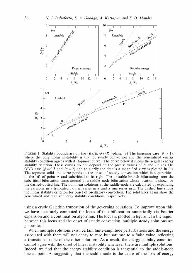
is discontininuous at the energy stability boundary. A closer look reveals a relativelyweak dependence of the bound on α. Indeed, the bound obtained for α = 0 is avery good approximation to the bound for other values of α. Figure 6 shows thedependence of the bound on α and β for fixed RT = 1000Rc, and illustrates againhow Nu∗ is only weakly sensitive to α in the limit of large β . Thus, we infer that, withthe constraints employed and the family of backgrounds chosen, the bound is notreduced on adding the stabilizing component in this limit. Perhaps Straus’ asymptoticsolution of the S-equation could be used to improve the situation.

5.3. Discontinuity in the bound

There are two obvious reasons why the bounds computed above could be discon-tinuous on the energy stability curve, neither of which is correct. First, a discontinuitycan arise due to the appearance of new finite-amplitude solutions in a saddle-nodebifurcation. Indeed, the loss of energy stability at the point where the saddle-node first


50

55

60

65

70

75

80

10

1.0

0.8

0.6

0.4

0.2

02 3 4 5 6 7

β

α

8 9

Figure 6. The bound (Numax) computed for the range 1.4 < β < 10 for RT = 1000Rc . The solidlines show contours of constant Numax for values of 81.5 (lowermost), 81, 80, 77.5, 75, 70, 65,60 and 55 (topmost).

appears (see figure 1) suggests that a jump of this kind might well be present aroundthese parameter settings. In this way, the bounding machinery could prove an effectivetool for exploring the nonlinear dynamics of the system. Unfortunately, it turns outthat the bound jumps discontinuously even in cases where there is no saddle-nodeand the energy stability condition coincides with linear onset (as for the fingeringcase). Moreover, no qualitative change occurs in the extent of the discontinuity whenwe approach parameter settings for which we know a saddle-node exists. Thus, thediscontinuity observed in our computations does not appear to be caused primarilyby the appearance of new nonlinear solutions.

The second reason why the bound could be discontinuous is that the backgroundprofiles change from being linear to piecewise linear on passing through the energystability curve. In fact, for this reason, discontinuities exist in bounds for thermalconvection. As shown by Doering & Constantin (1996), those discontinuities can beremoved by using a smoother background profile near the energy stability threshold,which raises the question of whether we can smooth out the current discontinuity bysimilar means.

To address this question one can return to the formulation of the variational prob-lem in § 4.2. Near the energy stability threshold, it is possible to develop asymptoticsolutions via perturbation theory without choosing a particular background. The finalvalue of the bound depends on integrals of various functions that are related to thebackground fields, and one could, in principle, optimize the procedure to find the bestbound. However, it becomes immediately clear on heading down this avenue that thebound always jumps discontinuous at the energy stability boundary, irrespective ofthe choice of background. The reason can be traced to the conditions in (4.21) which,in combination with the solution of the Euler–Lagrange equations in (4.20), leadto the optimal Nusselt number in (4.24). The trouble is that the matrix R becomessingular at the energy threshold (where q → 1 and ε → 0), and with the choice (4.21)already made, there is no way to adjust the background fields to ensure that Ψ ∗remains regular there. The result is that Nu∗ −1 always converges to a non-zero valueas RT approaches RT c from above. Given the failure of the perturbation expansion, itseems clear that the only possible way in which the discontinuity might be eliminatedis by avoiding one of the two extra assumptions made at the beginning of § 4.2(namely u∗ = 0 or (4.21)).


6. Discussion and open questionsIn this work, we have bounded fluxes in double-diffusive convection using the

Constantin–Doering–Hopf background method. Of particular interest is the behaviourof the bound for large Rayleigh numbers, where we find the dependence R

1/2T . This

bound is different from empirical flux laws often quoted in the literature (Turner1965), which show Nu ∼ R

1/3T . One reason for this discrepancy is that our bound may

simply be too conservative and grossly overestimate the physically realized flux, as canbe seen in comparison with the some numerical and asymptotic solutions (Radko &Stern 2000). Indeed, many examples of double-diffusive convection in the laboratoryand ocean show the formation of internal boundary layers (salt finger interfaces,diffusive steps), yet our optimal backgrounds only exhibit such sharp features nextto the walls and do not capture whatever process is responsible. However, as is alsotrue in Rayleigh–Benard problem, it is not clear whether the observed flows haveconverged to the ultimate asymptotic state of double-diffusive convection. If thatstate is characterized by flux laws which do not depend explicitly on the molecularvalues of diffusivity and viscosity, a 1/2 scaling law must eventually emerge.

A main difficulty addressed in this article is to account for the effect of thestabilizing element on the bound. This effect disappears from the most straightforwardimplementation of the background method, as it does from regular energy stabilitytheory. A similar problem is posed for geophysical and astrophysical systems in arotating frame of reference, where there is no effect of rotation rate in standardenergy stability theory and its extensions. The Prandtl number also plays no rolein the bounding theory of thermal as well as double-diffusive convection. The factthat the theory does not depend on these parameters does not mean that the systemis insensitive to them, but is merely a result of discarding the governing PDEs andkeeping only certain integral equations derived from them. Thus, the problem facingus is to add more integral constraints in order to incorporate the missing physics (seeIerley & Worthing 2001).

Here, we have identified and exploited a key constraint for doubly diffusive con-vection. The role of this constraint in energy stability theory is instructive, and amountsto generalizing the definition of the energy function so that one can suppress transientamplification in the absence of finite–amplitude instability. The constraint, however, isfar from sufficient in describing all the features of double-diffusive convection. In fact,the generalized energy stability threshold still seems to fall short of where we expectnonlinear solutions to come into existence. This leaves one suspicious that there maystill be inconsequential transient amplification above threshold, and prompts the twokey questions: Is it possible to differentiate between such transient growth and a truefinite-amplitude instability? Is it possible to improve energy analysis further so thatthe loss of energy stability always signifies a linear or nonlinear instability?

The bound we have derived is discontinuous along the energy stability boundary.Such jumps could reflect the appearance of additional finite-amplitude solutions atsaddle-node bifurcations, an eventuality that certainly occurs for double-diffusiveconvection. Unfortunately, our numerical computations offer little evidence that thisis the main cause of the discontinuity. The jump could also have been introducedbecause we have used piecewise linear background fields. Forcing the backgrounds tobe smooth removes any discontinuity of this kind in the Rayleigh–Benard problem.For the current problem, however, the difficulty is far more insidious: one canestablish for the simplified variational formulation in § 4.2 that the bound remainsdiscontinuous even for smooth background fields. The only remaining possibility for


further progress in using the bounding machinery to detect saddle-node bifurcationsis to retain the more general version variational problem in § 4.1.

Finally, the background method is geared towards extending energy stability theoryto find the properties of the solution with the biggest norm. While this methodhas provided us with some useful insight, other modifications of energy stabilitytheory must also be possible. In particular, it is conceivable that one may be ableto incorporate thresholds on the norm of perturbations that decay to the trivialstate, thus allowing one to extend the energy stability threshold for sufficiently ‘small’disturbances. Such a method could address important issues like the abrupt transitionto turbulence in some shear flows. Double-diffusive convection remains a rich testingground for all such future developments.

We acknowledge NSF grant ATM0222109 and a discovery NSERC grant forsupport. We thank Charles Doering and Richard Kerswell for discussions andsuggestions. The authors were hosted by the Department of Mathematics, MIT,and the GFD summer program, WHOI, at various times during this work and thehospitality is gratefully acknowledged.

Appendix. Energy stabilityStarting with (3.20), we consider two cases.

Case 1: β < 1

We substitute

λT = kT

√1 + β

1 − βand λS = kS

√β(1 + β)

1 − β(A 1)

into the constraint (3.17), to obtain

kT − 1

kT

= −α

(kS − 1

kS

). (A 2)

By letting A ≡ kS − 1/kS , (A 2) leads to the following relations:

kT =−αA ±

√α2A2 + 4

2and kS =

A ±√

A2 + 4

2. (A 3)

We seek the largest RT for nonlinear stability which satisfies (3.19). Therefore, wewould like to minimize |bT |. By substituting (A 1) and (A 3) in (3.12), we see that thebest choice to make |bT | as small as possible is when the signs of the second terms ofkT and kS in (A 3) are different. Therefore,

|bT | =1√

1 − β2|√

α2A2 + 4 − βα√

A2 + 4|. (A 4)

Case 1a: α � β

bT attains the minimum when

A2 =4

α2

β2 − α2

1 − β2,

which gives |bT | = 2√

1 − α2. From (3.19) and the definition of α, we obtain

RT − RS < Rc. (A 5)


Case 1b: β � α � 1/β

bT attains the minimum when A= 0, which gives bT = 2(1 − βα)/√

1 − β2. In thiscase, we obtain √

RT − β√

RS <√

1 − β2√

Rc. (A 6)

Case 1c: α � 1/β

In this case |bT | =0 because we may choose

A2 =4(β2α2 − 1)

1 − β2. (A 7)

Therefore, the system is nonlinear stable for all values of RT .

Case 2: β > 1

Here, we substitute

λT = kT

√β + 1

β − 1and λS = kS

√β(β + 1)

β − 1(A 8)

into the constraint (3.17) to obtain

kT +1

kT

= −α

(kS +

1

kS

). (A 9)

By letting A ≡ kS + 1/kS , (A 9) leads to the following relations:

kT =−αA ±

√α2A2 − 4

2and kS =

A ±√

A2 − 4

2. (A 10)

By substituting (A 8) and (A 10) in (3.12) and choosing different signs of the secondterms of kT and kS in (A 10), we obtain

|bT | =1√

β2 − 1|βα

√A2 − 4 −

√α2A2 − 4|. (A 11)

Case 2a: α < 1

|bT | attains the minimum when

A2 =4

α2

β2 − α2

β2 − 1,

which gives |bT | =2√

1 − α2. We then obtain

RT (1 − α2) < Rc (A 12)

or

RT − RS < Rc. (A 13)

Case 2b: α � 1

By substituting

A2 =4

α2

β2α2 − 1

β2 − 1,

in (A 11), we obtain |bT | =0. It is straightforward to show that α � 1 is a sufficientand necessary condition for A2 � 4. Therefore, the system is nonlinearly stable for allvalues of RT .


REFERENCES

Baggett, J. S., Driscoll, T. A. & Trefethen, L. N. 1993 A mostly linear model of transition toturbulence. Phys. Fluids 7, 833–838.

Baines, P. G. & Gill, A. E. 1969 On thermohaline convection with linear gradients. J. Fluid Mech.37, 289–306.

Bryan, F. 1986 High latitude salinity effects and interhemispheric thermohaline circulations. Nature323, 301–304.

Busse, F. H. 1969 On Howard’s upper bound for heat transport by turbulent convection. J. FluidMech. 37, 457–477.

Dijkstra, H. A., Te Raa, L. & Weijer, W. 2004 A systematic approach to determine thresholds ofthe ocean’s thermohaline circulation. Tellus 56, 362–370.

Doering, C. R. & Constantin, P. 1996 Variational bounds on energy dissipation in incompressibleflows. III. Convection. Phys. Rev. E 53, 5957–5981.

Howard, L. N. 1963 Heat transport by turbulent convection. J. Fluid Mech. 17, 405–432.

Ierley, G. R. & Worthing, R. A. 2001 Bound to improve: A variational approach to convectiveheat transport. J. Fluid Mech. 441, 223–253.

Jacobs, C. A., Huppert, H. E., Holdsworth, G. & Drewry, D. J. 1981 Thermohaline steps inducedby melting at the Erebus Glacier toungue. J. Geophys. Res. 86, 6547–6555.

Joseph, D. D. 1976 Stability of Fluid Motions, vol. II. Springer.

Kerswell, R. R. 1998 Unification of variational principles for turbulent shear flows: Thebackground method of Doering-Constantin and the mean-fluctuation formulation of Howard-Busse. Physica D 121, 175–192.

Lindberg, W. R. 1971 An upper bound on transport processes in turbulent thermohaline convection.J. Phys. Oceanogr. 1, 187–195.

Malkus, W. V. R. 1954 The heat transport and specturm of thermal turbulence. Proc. R. Soc. Lond.A 225, 196–212.

Merryfield, W. J. 2000 Origin of thermohaline staircases. J. Phys. Oceanogr. 30, 1046–1068.

Neal, V. T., Neshyba, S. & Denner, W. 1969 Thermal stratification in the Arctic Ocean. Science166, 373–374.

Nicodemus, R., Grossmann, S. & Holthaus, M. 1997 Improved variational principle for boundson energy dissipation in turbulent shear flow. Physica D 101, 178–196.

Plasting, S. C. & Kerswell, R. R. 2003 Improved upper bound on the energy dissipation rate inplane Couette flow: the full solution to Busse’s problem and the Constantin-Doering-Hopfproblem with one-dimensional background field. J. Fluid Mech. 477, 363–379.

Radko, T. & Stern, M. E. 2000 Finite-amplitude salt fingers in a vertically bounded layer. J. FluidMech. 425, 133–160.

Ruddick, B. 1992 Intrusive mixing in a Mediterranean salt lens - intrusion slopes and dynamicalmechanisms. J. Phys. Oceanogr. 22, 1274–1285.

Schmitt, R. W. 1994 Double diffusion in oceanography. Annu. Rev. Fluid Mech. 26, 255–285.

Spiegel, E. A. 1969 Semiconvection. Comm. Astrophys. Space Phys. 1, 57–60.

Stern, M. E. 1969 Collective instability of salt fingers. J. Fluid Mech. 35, 209–218.

Stern, M. E. 1982 Inequalities and variational-principles in double-diffusive turbulence. J. FluidMech. 114, 105–121.

Stocker, T. F. 1999 Abrupt climate changes: from the past to the future - a review. Intl J. EarthSci. 88, 365–374.

Straus, J. M. 1973 Upper bound on the solute flux in double diffusive convection. Phys. Fluids 17,520–527.

Turner, J. S. 1965 Buoyancy Effects in Fluids. Cambridge University Press.

Tziperman, E. & Ioannou, P. J. 2002 Transient growth and optimal excitation of thermohalinevariability. J. Phys. Oceanogr. 32, 3427–3435.

Ulrich, R. K. 1972 Thermohaline convection in stellar interiors. Astrophys. J. 172, 165–177.

Vauclair, S. 2004 Thermohaline convection and metallic fingers in polluted stars. In The A-StarPuzzle (ed. J. Zverko, J. Ziznovsky, S. Adelman & W. Weiss), Proc. IAU Symposium 224,p. 161–166.

Veronis, G. 1965 On finite amplitude instability in thermohaline convection. J. Mar. Res. 23, 1–17.

Waleffe, F. 1995 Transition in shear flows – Nonlinear normality versus nonnormal linearity. Phys.Fluids 7, 3060–3066.

Documents

Bounds on double-diffusive convection - Mathematics, Department of