arX

iv:0

907.

4918

v1 [

phys

ics.

clas

s-ph

] 2

8 Ju

l 200

9

BOUSSINESQ SYSTEMS OF BONA-SMITH TYPE ON

PLANE DOMAINS: THEORY AND NUMERICAL ANALYSIS∗

V. A. Dougalis †‡, D. E. Mitsotakis§and J.-C. Saut §

September 3, 2018

Abstract

We consider a class of Boussinesq systems of Bona-Smith type in two space dimensions approxi-

mating surface wave flows modelled by the three-dimensional Euler equations. We show that various

initial-boundary-value problems for these systems, posed on a bounded plane domain are well posed

locally in time. In the case of reflective boundary conditions, the systems are discretized by a modi-

fied Galerkin method which is proved to converge in L2 at an optimal rate. Numerical experiments

are presented with the aim of simulating two-dimensional surface waves in complex plane domains

with a variety of initial and boundary conditions, and comparing numerical solutions of Bona-Smith

systems with analogous solutions of the BBM-BBM system.

1 Introduction

In this paper we will study the Boussinesq system

ηt +∇ · v +∇ · ηv − b∆ηt = 0,

vt +∇η + 12∇|v|2 + c∇∆η − b∆vt = 0,

(1.1)

where b > 0 and c < 0 are constants. This system is the two-dimensional version of a system in one space

variable originally derived and analyzed by Bona and Smith, [BS]. It belongs to a family of Boussinesq

∗This work was supported in part by a French-Greek scientific cooperation grant for the period 2006–08, funded jointly

by EGIDE, France, and the General Secretariat of Research and Technology, Greece. D. Mitsotakis was also supported by

Marie Curie Fellowship No. PIEF-GA-2008-219399 of the European Commission.†Department of Mathematics, University of Athens, 15784 Zographou, Greece‡Institute of Applied and Computational Mathematics FO.R.T.H., 70013 Heraklion, Greece§UMR de Mathematiques, Universite de Paris-Sud, Batiment 425, 91405 Orsay, France

1

systems, [BCSI], [BCL], that approximate the three-dimensional Euler equations for the irrotational free

surface flow of an ideal fluid over a horizontal bottom. In (1.1) the independent variables x = (x, y)

and t represent spatial position and elapsed time, respectively. The dependent variables η = η(x, t) and

v = v(x, t) = (u(x, t), v(x, t)), represent quantities proportional, respectively, to the deviation of the free

surface from its level of rest, and to the horizontal velocity of the fluid particles at some height above the

bottom. In (1.1) the variables are nondimensional and unscaled and the horizontal velocity v is evaluated

at a height z = −1 + θ(1 + η(x, t)), for some θ ∈ [√2/3, 1]. (In these variables the bottom lies at height

z = −1.) In terms of the parameter θ, the constants in (1.1) are given by the formulas b = (3θ2 − 1)/6

and c = (2− 3θ2)/3. (The system originally analyzed by Bona and Smith in [BS] corresponds to θ2 = 1.)

The value θ2 = 2/3 (i.e. c = 0) yields the BBM-BBM system, [BC], [DMSII], [Ch].

The system (1.1) is derived from the Euler equations, [BCSI], [BCL], under a long wavelength, small

amplitude assumption. Specifically, one assumes that ε := A/h0 ≪ 1, λ/h0 ≫ 1 with the Stokes number

S := Aλ2/h30 being of O(1). (Here A is the maximum amplitude of the surface waves measured over

the level of rest, z = −h0 is the (constant) depth of the bottom, and λ is a typical wavelength.) If one

takes S = 1, then, in nondimensional, scaled variables, appropriate asymptotic expansions in the Euler

equations yield equations of the form

ηt +∇ · v + ε(∇ · ηv − b∆ηt) = O(ε2),

vt +∇η + ε(12∇|v|2 + c∇∆η − b∆vt

)= O(ε2),

(1.2)

from which (1.1) follows by unscaling to remove ε, and replacing the right-hand side by zero.

The Cauchy problem for (1.1) in the case of one spatial variable has been proved to be globally well

posed for 2/3 < θ2 ≤ 1 in appropriate classical and Sobolev space pairs, [BS], [BCSI]. The analogous

problem for θ2 = 2/3 is locally well posed, [BCSI]. In [DMSI] we considered a more general class of systems

in the two-dimensional case and proved that the corresponding Cauchy problem is locally well posed in

appropriate pairs of Sobolev spaces. Initial-boundary-value problems (ibvp’s) for (1.1) for 2/3 ≤ θ2 ≤ 1

on a finite interval in one space variable were analyzed in [ADMI], and in [BC] for θ2 = 2/3. It was proved

in [ADMI] that the ibvp with Dirichlet boundary conditions, wherein η and u are given functions of t

at the endpoints of the interval, is locally well posed. The corresponding ibvp with reflection boundary

conditions (ηx = u = 0 at both endpoints of the interval) was shown in [ADMI] to be globally well posed;

so is also the periodic ivp. In [DMSII] we analyzed three ibvp’s for the BBM-BBM system on a smooth

plane domain Ω, corresponding to homogeneous Dirichlet boundary conditions for η and v on ∂Ω, to

2

homogeneous Neumann boundary conditions for η and v on ∂Ω, and to the (normal) reflective boundary

conditions ∂η∂n = 0, and v = 0 on ∂Ω, where n is the normal direction to the boundary. We showed that

these ibvp’s are well posed locally in time in the appropriate sense.

In Section 2 of the paper at hand we consider the Bona-Smith system (1.1) and pose it as an ibvp on a

plane domain Ω under a variety of homogeneous boundary conditions on ∂Ω, including e.g. homogeneous

Dirichlet b.c.’s for η and v and reflective b.c.’s. We prove that the corresponding ibvp’s are well posed,

locally in time.

Turning now to the numerical solution of ibvp’s for systems of the type (1.1) by Galerkin-finite

element methods, we note first that it is quite straightforward to construct and analyze such schemes

for the BBM-BBM system. For example, in [DMSI] we proved optimal-order L2-error estimates for the

standared Galerkin semidiscretization of the BBM-BBM system with homogeneous boundary conditions

on a smooth domain with a general triangulation. When c > 0, i.e. in the case of the proper Bona-Smith

systems, the presence of the term ∇∆η complicates issues. In [DMSI] we analyzed the standard Galerkin

semidiscretization with bicubic splines for this class of systems posed on rectangles with homogeneous

Dirichlet boundary conditions, and proved optimal-order H2-error estimates for the approximation of η.

(Experimental evidence indicates that the L2-errors for the approximation of η, u and v with this scheme

have suboptimal – O(h3) – rate of convergence. In the one-dimensional case one may derive optimal-order

estimates for the approximations of η, u, v in W 1,∞ × L∞ × L∞, cf. [ADMII].)

In Section 3 of the present paper we consider the Bona-Smith systems with c > 0 posed on convex

smooth planar domains with reflective boundary conditions. The systems are discretized on an arbitrary

triangulation of the domain using a modified Galrkin method, wherein the Laplacian in the ∇∆η terms

in (1.1) is discretized weakly by an appropriate discrete Laplacian operator. This enables us to prove

optimal-order L2- andH1- error estimates on finite element subspaces of continuous, piecewise polynomial

functions that include the case of piecewise linear functions utilized in most applications. The systems of

ordinary differential equations representing the semidiscretizations of the Bona-Smith systems are shown

to be non-stiff. One may thus use any explicit method for their temporal discretization.

We close the paper by showing the results of a series of numerical experiments of simulations of

surface waves in complex domains, aimed at comparing the numerical solution of a Bona-Smith system

with analogous results obtained by solving the BBM-BBM system.

3

2 Well-posedness of ibvp’s for the Bona-Smith system

Let Ω be a bounded plane domain with smooth boundary (or a convex polygon). We consider the

Bona-Smith system

ηt +∇ · (v + ηv) − b∆ηt = 0, (2.1a)

vt +∇

(η +

1

2|v|2 + c∆η

)− b∆vt = 0, (2.1b)

for (x, t) ∈ Ω× R+, with b > 0, c < 0, with initial conditions

η(x, 0) = η0(x), v(x, 0) = v0(x) x ∈ Ω. (2.2)

We now describe the class of boundary conditions on ∂Ω under which the problem (2.1)–(2.2) will

be solved. Let Hs = Hs(Ω), s ∈ R, denote the L2-based, real-valued, Sobolev classes on Ω and H10 the

subspace of H1 whose elements have zero trace on ∂Ω. In the sequel, we shall denote by ‖ · ‖ and (·, ·)

the norm and inner product, respectively, of L2 = L2(Ω), by ‖ · ‖s the norm of Hs, and by ‖ · ‖∞ the

norm of L∞ = L∞(Ω). The boundary conditions on η will be of the form

Bη = 0, x ∈ ∂Ω, t ∈ R+, (2.3a)

where the linear operator B and the domain Ω will be assumed to be such that the boundary-value

problem

−b∆w + w = f, in Ω,

Bw = 0, in ∂Ω,

has for each f in L2 a unique solution w ∈ H2 for which Bw|∂Ω is well defined. (We will also assume

that an H1 solution w of the problem is defined whenever f ∈ H−1). The boundary conditions on v will

be of homogeneous Dirichlet type, i.e.

v = 0, x ∈ ∂Ω, t ∈ R+. (2.3b)

We note that examples of suitable boundary conditions of the type (2.3a) include, among other, homo-

geneous Dirichlet (η = 0), Neumann ( ∂η∂n = 0) or Robin (α ∂η∂n + βη = 0) boundary conditions on the

4

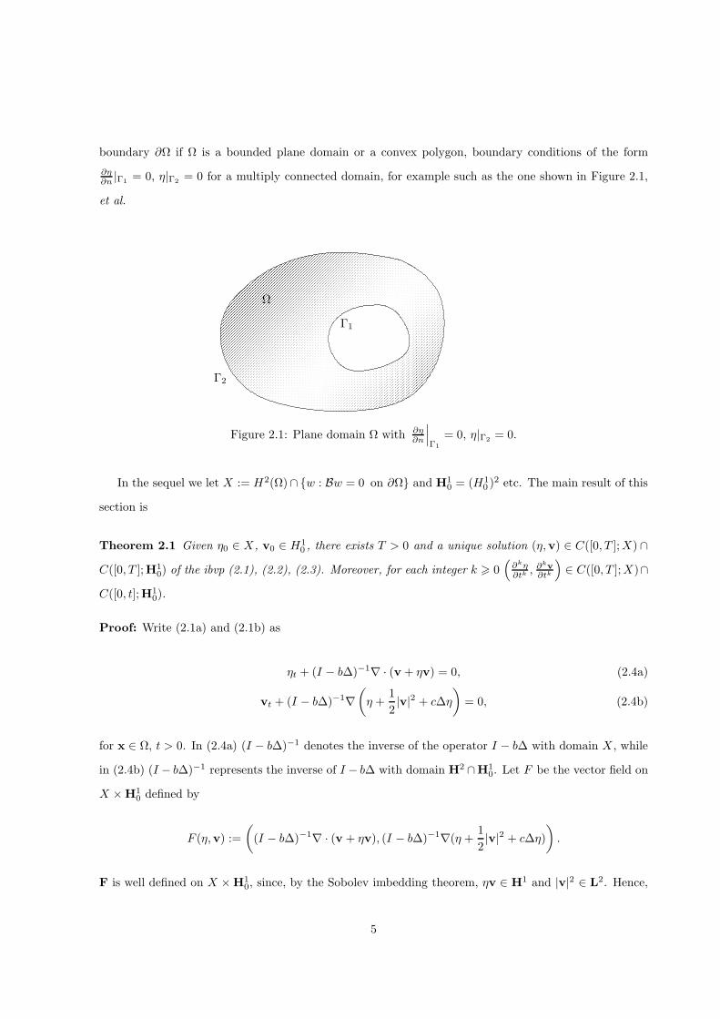
boundary ∂Ω if Ω is a bounded plane domain or a convex polygon, boundary conditions of the form

∂η∂n |Γ1

= 0, η|Γ2= 0 for a multiply connected domain, for example such as the one shown in Figure 2.1,

et al.

Ω

Γ1

Γ2

Figure 2.1: Plane domain Ω with ∂η∂n

∣∣∣Γ1

= 0, η|Γ2= 0.

In the sequel we let X := H2(Ω)∩ w : Bw = 0 on ∂Ω and H10 = (H1

0 )2 etc. The main result of this

section is

Theorem 2.1 Given η0 ∈ X, v0 ∈ H10 , there exists T > 0 and a unique solution (η,v) ∈ C([0, T ];X) ∩

C([0, T ];H10) of the ibvp (2.1), (2.2), (2.3). Moreover, for each integer k > 0

(∂kη∂tk

, ∂kv

∂tk

)∈ C([0, T ];X)∩

C([0, t];H10).

Proof: Write (2.1a) and (2.1b) as

ηt + (I − b∆)−1∇ · (v + ηv) = 0, (2.4a)

vt + (I − b∆)−1∇

(η +

1

2|v|2 + c∆η

)= 0, (2.4b)

for x ∈ Ω, t > 0. In (2.4a) (I − b∆)−1 denotes the inverse of the operator I − b∆ with domain X , while

in (2.4b) (I − b∆)−1 represents the inverse of I − b∆ with domain H2 ∩H10. Let F be the vector field on

X ×H10 defined by

F (η,v) :=

((I − b∆)−1∇ · (v + ηv), (I − b∆)−1∇(η +

1

2|v|2 + c∆η)

).

F is well defined on X ×H10, since, by the Sobolev imbedding theorem, ηv ∈ H1 and |v|2 ∈ L2. Hence,

5

(I − b∆)−1∇ · (v + ηv) ∈ X and (I − b∆)−1∇(η + 12 |v|

2 + c∆η) ∈ H10. Moreover, F is C1 on X ×H1

0,

with derivative F ′(η∗,v∗) given by

F ′(η∗,v∗)(η,v) =((I − b∆)−1∇ · (v + ηv∗ + η∗v), (I − b∆)−1∇(η + v∗ · v + c∆η)

).

The continuity of F ′ follows from the Sobolev imbedding theorem and the regularity properties of the

operators (I − b∆)−1, considered as inverses of (I − b∆) on X for the first component, and of I − b∆ on

H2 ∩H10 for the second.

By the standard theory of ordinary differential equations in Banach spaces, we conclude therefore that

there exists a unique maximal solution (η,v) ∈ C1([0, T ];X) × C1([0, T ];H10) of (2.4) for some T > 0,

with η|t=0 = η0 and v|t=0 = v0. The first conclusion of the theorem follows. The assertion on ∂kη∂tk ,

∂kv

∂tk

follows by differentiating (2.4) with respect to t k − 1 times.

Remark 2.1 It is not hard to see, using the energy method on the nondimensional but scaled system

(1.2) (with right-hand side replaced by zero), that at least in the cases of homogeneous Dirichlet boundary

conditions for η and v and reflective boundary conditions ∂η∂n = 0, v = 0 on ∂Ω, the maximum existence

time Tε is independent of ε.

Remark 2.2 If the domain Ω is smooth, one gets smooth solutions from smooth data. Namely, let

k ∈ N, k ≥ 3, and assume that η0 ∈ X ∩ Hk, v0 ∈ H10 ∩ Hk−1, then (η,v) ∈ C([0, T ];X ∩ Hk) ∩

C([0, T ];H10 ∩Hk−1). This follows directly from the elliptic regularity estimates on I − b∆ (with the ad

hoc boundary conditions). One is thus reduced to an ODE in X ∩Hk ×H10 ∩Hk−1.

Remark 2.3 Consider the ibvp (2.1)–(2.2) for the Bona-Smith system with (normal) reflective bound-

ary conditions

∂η

∂n= 0, v = 0, for x ∈ ∂Ω, t ∈ R+. (2.5)

It is known that in one dimension, cf. [ADMI], the Hamiltonian of the ibvp (2.1), (2.2), (2.5),

H = H(η,v) =1

2

∫

Ω

[η2 + (1 + η)|v|2 − c|∇η|2

]dx, (2.6)

is conserved. (Indeed this implies global existence-uniqueness of the solution of this ibvp in 1D provided

that η0(x) + 1 > 0 and H(η0, u0) is suitably restricted.) In the two-dimensional case H is not conserved

6

in general. To see this, write the system (2.1) for (x, t) ∈ Ω× R+ as

ηt +∇ ·P = 0, (2.7a)

vt +∇Q + b∇× ωt = 0, (2.7b)

where P := v + ηv − b∇ηt, Q := η + 12 |v|

2 + c∆η − b∇ · vt, and ω is the vorticity of the flow given by

ω = ∇× v = (0, 0, ω), ω := vx − uy. From (2.7) we obtain

∫

Ω

[ηtQ+ vt ·P+∇ · (QP) + bP · (∇× ωt)] dx = 0 (2.8)

Using now the reflective boundary conditions in (2.8) and integrating by parts we see that in the maximal

temporal interval of existence of a solution of the ibvp (2.1), (2.2), (2.5),

dH

dt+ b

∫

Ω

P · (∇× ωt)dx = 0. (2.9)

Hence, a simple sufficient condition for the conservation of the Hamiltonian is irrotationality of the flow.

In one space dimension, the flow is trivially irrotational. In 2D taking the curl of (2.1a) we see that

∂t(ω − b∆ω) = 0, t > 0. (2.10)

Now, if the flow is, for example, irrotational at t = 0, the reflective boundary conditions do not allow

us to conclude from (2.10) that ω = 0 for t > 0. However, in the case of the Cauchy problem or the

ibvp with periodic boundary conditions on η and v on a rectangle (wherein (2.8) holds as well), ω(0) = 0

implies by (2.10) that ω = 0 for t > 0. (This was also noticed for the BBM-BBM system in [CI].) In

these cases, it follows by (2.9) that the Hamiltonian is invariant. Note however that conservation of H

does not imply global well-posedness in 2D.

3 A modified Galerkin method

We turn now to the numerical solution of the ibvp (2.1), (2.2), (2.5) by Galerkin-finite element methods.

The usual Galerkin method for Bona-Smith systems that was analyzed in [DMSI] requires finite element

subspaces consisting of C2 functions. Hence, it is not very useful in practice, as it cannot be applied to

arbitrary plane domains and triangulations. In this section a modified Galerkin method for the numerical

7

solution of the ibvp with (normal) reflection boundary conditions is analyzed. The method is more

versatile, being applicable to general triangulations and domains (even with piecewise linear continuous

functions) and is shown to have error estimates with optimal convergence rates in L2 and H1.

For ease of reference we rewrite here the ibvp that we will approximate. We seek η and v, defined for

(x, t) ∈ Ω× [0, T ] and satisfying for constants b > 0 and c ≤ 0

ηt +∇ · v +∇ · ηv − b∆ηt = 0,

vt +∇(η + 12 |v|

2 + c∆η)− b∆vt = 0,(x, t) ∈ Ω× [0, T ],

η(x, 0) = η0(x), v(x, 0) = v0(x), x ∈ Ω,

∂η∂n (x, t) = 0, v(x, t) = 0, (x, t) ∈ ∂Ω× [0, T ].

(R)

We assume that Ω is a convex domain with smooth enough boundary ∂Ω and that the ibvp (R) has a

unique solution (η,v) which is smooth enough for the purposes of its numerical approximation. In the

sequel, we put x = (x, y).

We suppose that Th is a regular triangulation of Ω with triangles τ of maximum sidelength h and let

Sh be a finite-dimensional subspace of C(Ω) ∩H1, which, for small enough h and integer r ≥ 2, satisfies

the approximation property

infχ∈eSh

‖w − χ‖+ h‖w − χ‖1 ≤ Chs‖w‖s, 1 ≤ s ≤ r, (3.1)

when w ∈ Hs. (In this section C will denote generic constants independent of h.) On the same triangu-

lation we denote by Sh the subspace of Sh consisting of the elements of Sh that vanish on the boundary

i.e. Sh = Sh ∩H10 . Hence, on Sh we have

infχ∈Sh

‖w − χ‖+ h‖w − χ‖1 ≤ Chs‖w‖s, 1 ≤ s ≤ r, (3.2)

for w ∈ Hs ∩ H10 . We will assume that the elements of Sh and Sh are piecewise polynomial functions

defined on Th, of degree at most r − 1 on each τ ∈ Th.

We consider the symmetric bilinear form aD : H10 ×H1

0 → R defined by

aD(u, v) := (u, v) + b(∇u,∇v), u, v ∈ H10 , (3.3)

which is coercive on H10 ×H1

0 . In addition, we consider the symmetric bilinear form aN : H1 ×H1 → R

8

that is defined by

aN (u, v) := (u, v) + b(∇u,∇v), u, v ∈ H1, (3.4)

and is coercive on H1×H1. With the aid of aD, aN we define the elliptic projection operators Rh : H10 →

Sh, Rh : H1 → Sh as follows:

aD(Rhw, χ) = aD(w, χ), ∀w ∈ H10 , χ ∈ Sh, (3.5a)

aN (Rhw, χ) = aN (w, χ), ∀w ∈ H1, χ ∈ Sh. (3.5b)

As a consequence of (3.1), (3.2) and elliptic regularity we have then

‖w −Rhw‖k ≤ Chs−k‖w‖s, w ∈ Hs ∩H10 , 2 ≤ s ≤ r, k = 0, 1, (3.6a)

and

‖w − Rhw‖k ≤ Chs−k‖w‖s, w ∈ Hs, 2 ≤ s ≤ r, k = 0, 1. (3.6b)

We assume that the triangulation Th is quasiuniform. Then, the following inverse assumptions hold on

Sh, [Ci]

‖χ‖1 ≤ Ch−1‖χ‖, ∀χ ∈ Sh, (3.7)

‖χ‖∞ ≤ Ch−1‖χ‖, ∀χ ∈ Sh, (3.8)

The same inverse assumptions hold on Sh as well.

We will also assume that for the elliptic projections we have the following approximation properties

in the L∞ norm:

‖w −Rhw‖∞ ≤ Cγ(h)‖w‖r,∞, ∀w ∈ W r∞ ∩H1

0 , (3.9a)

‖w − Rhw‖∞ ≤ Cγ(h)‖w‖r,∞, ∀w ∈W r∞, (3.9b)

where γ(h) = hr| log h|r with r = 0 if r > 2 and r = 1 when r = 2, cf. [S]. Here, W r∞ (with norm ‖ · ‖r,∞)

denotes the L∞-based Sobolev space on Ω of order r.

9

In the sequel we will use the discrete Laplacian operator ∆h : H1 → Sh, defined for w ∈ H1 by

(∆hw, χ) = −(∇w,∇χ), ∀χ ∈ Sh. (3.10)

By the divergence theorem, it is easy to check that for w ∈ H2 there holds

(∆hRhw, χ) = (∆w, χ) −

∫

∂Ω

∂w

∂nχds−

1

b(w, χ) +

1

b(Rhw, χ), χ ∈ Sh. (3.11)

Hence, if w ∈ H2 with ∂w∂n |∂Ω = 0, then

∆hRhw = Ph∆w +1

b(Rh − Ph)w, (3.12)

where Ph is the L2-projection onto Sh. The identity (3.11) is proved as follows: For w ∈ H2, χ ∈ Sh,

using the definition of Rh we have

(∆hRhw, χ) = −(∇Rhw,∇χ)−1

b(Rhw, χ) +

1

b(Rhw, χ)

= −(∇w,∇χ)−1

b(w, χ) +

1

b(Rhw, χ),

= −

∫

∂Ω

∂w

∂nχds+ (∆w, χ) −

1

b(w, χ) +

1

b(Rhw, χ).

Denoting the components of v as (u, v), we define the semidiscrete modified Galerkin method as follows.

We seek ηh : [0, T ] → Sh, uh, vh : [0, T ] → Sh, approximations to η, u, v, respectively, such that

aN (ηht, φ) + (uhx, φ) + (vhy, φ) + ((ηhuh)x, φ) + ((ηhvh)y, φ) = 0, φ ∈ Sh,

aD(uht, χ) + (ηhx, χ) + (uhuhx, χ) + (vhvhx, χ) + c((∆hηh)x, χ) = 0, χ ∈ Sh,

aD(vht, ψ) + (ηhy, ψ) + (uhuhy, ψ) + (vhvhy, ψ) + c((∆hηh)y, ψ) = 0, ψ ∈ Sh,

ηh(·, 0) = Rhη0, uh(·, 0) = Rhu0, vh(·, 0) = Rhv0.

0 ≤ t ≤ T, (3.13)

These relations are discrete analogs to the corresponding variational forms of the first p.d.e. of (R) in

H1 and of the second in (H10 )

2. Note that since ηhuh ∈ C(Ω), ηhuh|τ ∈ C∞(τ) for each τ ∈ Th, and

ηhuh|∂Ω = 0, it follows that ηhuh ∈ H10 . Similarly, ηhvh ∈ H1

0 , u2h ∈ H1

0 , v2h ∈ H1

0 . Hence, all terms in

the inner products of (3.13) are well defined. We now consider the mappings fx, fy : L2 → Sh defined for

10

w ∈ L2 by:

aD(fx(w), φ) = (w, φx), φ ∈ Sh,

aD(fy(w), φ) = (w, φy), φ ∈ Sh,

and the mappings and gx.gy : L2 → Sh defined for w ∈ L2 by

aN (gx(w), χ) = (w, χx), χ ∈ Sh,

aN (gy(w), χ) = (w, χy), χ ∈ Sh.

Then (3.13) can be written as

ηht = F (uh, vh, ηh),

uht = G(uh, vh, ηh), 0 ≤ t ≤ T

vht = Z(uh, vh, ηh),

ηh(0) = Rhη0, uh(0) = Rhu0, vh(0) = Rhv0,

(3.14)

where

F (uh, vh, ηh) := gx(uh) + gy(vh) + gx(ηhuh) + gy(ηhvh),

G(uh, vh, ηh) := fx(ηh) +1

2(fx(u

2h) + fx(v

2h)) + cfx(∆hηh),

Z(uh, vh, ηh) := fy(ηh) +1

2(fy(u

2h) + fy(v

2h)) + cfy(∆hηh).

For the mappings fx, fy, gx and gy we have the following stability estimates:

Lemma 3.1 There exists a constant C such that

(i) ‖fx(w)‖1 ≤ C‖w‖, and ‖fy(w)‖1 ≤ C‖w‖, w ∈ L2.

(ii) ‖gx(w)‖1 ≤ C‖w‖, and ‖gy(w)‖1 ≤ C‖w‖, w ∈ L2.

Proof: The proof follows immediately from the coercivity of aD on H10 ×H1

0 and of aN on H1×H1 and

the definitions of fx, fy, gx, gy.

11

We define now the negative norms ‖ · ‖−1 and ‖ · ‖−2 for functions w ∈ L2 as

‖w‖−1 := supz∈H1

z 6=0

(w, z)

‖z‖1and ‖w‖−2 := sup

z∈H2∩H1

0

z 6=0

(w, z)

‖z‖2.

Lemma 3.2 There exists a constant C > 0 such that

‖fx(χ)‖ ≤ C‖χ‖−1, ‖fy(χ)‖ ≤ C‖χ‖−1, ∀χ ∈ Sh. (3.15)

Proof: Let χ ∈ Sh. Consider the problem Lw = χx with w = 0 on ∂Ω, where L := I − b∆ with domain

H2 ∩H10 . Then, by elliptic regularity and denoting by L−1 the inverse of L, we have

‖χx‖−2 = sup06=z∈H2∩H1

0

(χx, z)

‖z‖2= sup

06=z∈H2∩H1

0

(Lw, z)

‖z‖2

≥(Lw,L−1w)

‖L−1w‖2=

‖w‖2

‖L−1w‖2≥ C

‖w‖2

‖w‖

= C‖w‖. (3.16)

Let now 0 6= z ∈ H2 ∩H10 . Then

(χx, z)

‖z‖2=

−(χ, zx)

‖z‖2≤

‖χ‖−1‖zx‖1‖z‖2

≤ ‖χ‖−1.

Hence

sup06=z∈H2∩H1

0

(χx, z)

‖z‖2≤ ‖χ‖−1.

Therefore

‖χx‖−2 ≤ ‖χ‖−1,

and by (3.15)

‖w‖ ≤ C‖χ‖−1. (3.17)

Consider Rhw, the elliptic projection of w onto Sh. Note that Rhw = fx(χ). In addition, by (3.6a)

‖Rhw − w‖ ≤ Ch2‖w‖2 ≤ Ch2‖χx‖ ≤ Ch2h−2‖χ‖−1 = C‖χ‖−1.

(In the last inequality we used the inverse inequality ‖ϕ‖1 ≤ Ch−2‖ϕ‖−1, ∀ϕ ∈ Sh, which is valid since

12

by (3.7):

‖ϕ‖−1 = sup06=z∈H1

(ϕ, z)

‖z‖1≥

‖ϕ‖2

‖ϕ‖1≥ Ch2

‖ϕ‖21‖ϕ‖1

= Ch2‖ϕ‖1.)

We conclude that

‖Rhw‖ − ‖w‖ ≤ ‖Rhw − w‖ ≤ C‖χ‖−1,

and by (3.17)

‖fx(χ)‖ = ‖Rhw‖ ≤ C‖χ‖−1,

which is the required conclusion. The proof for fy is entirely analogous.

Lemma 3.3 There exists a constant C such that

‖∆hu‖−1 ≤ C‖∇u‖, ∀u ∈ H1. (3.18)

Proof: Let u ∈ H1. Then, for each w 6= 0 ∈ H1 we have

(∆hu,w)

‖w‖1=

(∆hu, Phw)

‖w‖1≤

‖∇u‖‖∇Phw‖

‖w‖1≤ C‖∇u‖,

from which, taking the supremum over w ∈ H1 we obtain (3.18). We used the stability of Ph on H1, i.e.

the inequality

‖Phw‖1 ≤ C‖w‖1, forw ∈ H1,

which follows by the argument in [CT].

We now state and prove the main result of this section.

Theorem 3.1 For h sufficiently small, the semidiscrete problem (3.14) has a unique solution (ηh, uh, vh)

in the interval [0, T ] of maximal existence of the solution (η, u, v) of the ibvp (R). Moreover, for some

constant C = C(η, u, v, T ) independent of h we have

‖η − ηh‖+ ‖u− uh‖+ ‖v − vh‖ ≤ Chr,

and

‖η − ηh‖1 + ‖u− uh‖1 + ‖v − vh‖1 ≤ Chr−1,

for each t ∈ [0, T ].

13

Proof: We suppose that for some constant M there holds that ‖η‖∞ ≤M , ‖u‖∞ ≤ M and ‖v‖∞ ≤ M

for 0 ≤ t ≤ T . Then, from (3.9b) for h sufficiently small

‖η0h‖∞ ≤ ‖η0h − η0‖∞ + ‖η0‖∞ = ‖Rhη0 − η0‖∞ + ‖η0‖∞ ≤ Cγ(h)‖η0‖r,∞ + ‖η0‖∞ < 2M.

Similar estimates hold for u0h and v0h. The o.d.e. system (3.14) has a unique solution locally in t. By

continuity, we may assume that there exists th ∈ (0, T ] such that ‖uh‖∞ ≤ 2M , ‖ηh‖∞ ≤ 2M and

‖vh‖∞ ≤ 2M for all t ≤ th.

We let now

ρ = η − Rhη, θ = Rhη − ηh, τ = v −Rhv, ζ = Rhv − vh, σ = u−Rhu, ξ = Rhu− uh,

so that θ ∈ Sh, ζ, ξ ∈ Sh and η− ηh = ρ+ θ, u− uh = σ + ξ, v − vh = τ + ζ. By (R) and (3.14) we have

θt = gx(σ + ξ) + gy(τ + ζ) + gx(uη − uhηh) + gy(vη − vhηh), (3.19)

ξt = fx(θ + ρ) +1

2

fx(u

2)− fx(u2h) + fx(v

2)− fx(v2h)+ cfx(∆η − ∆hηh), (3.20)

ζt = fy(τ + ζ) +1

2

fy(u

2)− fy(u2h) + fy(v

2)− fy(v2h)+ cfy(∆η − ∆hηh). (3.21)

The equation (3.20) may be written as

ξt = fx(θ + ρ) +1

2

fx(u(σ + ξ)) + fx((σ + ξ)uh) + fx(v(τ + ζ)) + fx((τ + ζ)vh)

+ cfx(∆η − ∆hηh).

Taking L2-norms and using Lemma 3.1, (3.15), (3.12), (3.6a), (3.6b) and (3.18) we obtain, for 0 ≤ t ≤ th,

‖ξt‖ ≤ ‖fx(θ + ρ)‖+1

2

(‖fx(u(σ + ξ))‖+

‖fx((σ + ξ)uh)‖+ ‖fx(v(τ + ζ))‖ + ‖fx((τ + ζ)vh)‖)+ ‖cfx(∆η − ∆hηh)‖

≤ C(‖θ + ρ‖+ ‖u(σ + ξ)‖ + ‖(σ + ξ)uh‖+ ‖v(τ + ζ)‖ + ‖(τ + ζ)vh‖+

‖fx(∆η − ∆hRhη)‖+ ‖fx(∆h(Rhη − ηh)‖)

≤ C[‖θ‖+ ‖ρ‖+ ‖u‖L∞(‖σ‖+ ‖ξ‖) + ‖v‖L∞(‖τ‖ + ‖ζ‖) +

‖vh‖L∞(‖τ‖+ ‖ζ‖) + ‖uh‖L∞(‖σ‖+ ‖ξ‖) + ‖∆η − ∆hRhη‖+ ‖∆h(Rhη − ηh)‖−1]

≤ C[hr + ‖θ‖+ ‖ξ‖+ ‖ζ‖+ ‖∆η − Ph∆η‖+ ‖Rhη − Phη‖+ ‖Rhη − ηh‖1

],

14

and so

‖ξt‖ ≤ C(hr + ‖θ‖1 + ‖ξ‖+ ‖ζ‖). (3.22)

Similarly, we have for 0 ≤ t ≤ th

‖ζt‖ ≤ C(hr + ‖θ‖1 + ‖ξ‖+ ‖ζ‖). (3.23)

The equation (3.19) may be written as

θt = gx(σ + ξ) + gy(τ + ζ) + gx(u(ρ+ θ)) + gx((σ + ξ)ηh) + gy(v(ρ+ θ)) + gy((τ + ζ)ηh).

Hence, taking H1-norms and using Lemma 3.1, and (3.6a,b) we have for 0 ≤ t ≤ th

‖θt‖1 ≤ C(‖σ + ξ‖+ ‖τ + ζ‖

+‖u(ρ+ θ)‖ + ‖(σ + ξ)ηh‖+ ‖v(ρ+ θ)‖ + ‖(τ + ζ)ηh‖)

≤ C(‖σ‖+ ‖ξ‖+ ‖τ‖+ ‖ζ‖+ ‖u‖L∞(‖ρ‖+ ‖θ‖) + (‖σ‖+ ‖ξ‖)‖ηh‖L∞

+‖v‖L∞(‖ρ‖+ ‖θ‖) + (‖τ‖+ ‖ζ‖)‖ηh‖L∞)

≤ C(‖σ‖+ ‖ξ‖+ ‖τ‖+ ‖ζ‖+ ‖ρ‖+ ‖θ‖),

and therefore that

‖θt‖1 ≤ C(hr + ‖θ‖+ ‖ξ‖+ ‖ζ‖), 0 ≤ t ≤ th. (3.24)

From (3.22)–(3.24) we see that for 0 ≤ t ≤ th

1

2

d

dt(‖θ‖21 + ‖ξ‖2 + ‖ζ‖2) ≤ Ch2r + C(‖θ‖21 + ‖ξ‖2 + ‖ζ‖2),

from which, using Gronwall’s inequality, we have for 0 ≤ t ≤ th

‖θ‖1 + ‖ξ‖+ ‖ζ‖ ≤ Chr. (3.25)

Hence, for t ≤ th there holds

‖η − ηh‖+ ‖u− uh‖+ ‖v − vh‖ ≤ Chr. (3.26)

15

Furthermore for t ≤ th, we have, by (3.8), (3.9b) and (3.25)

‖ηh − η‖L∞ ≤ ‖ηh − Rhη‖L∞ + ‖Rhη − η‖L∞

≤ Ch−1‖ηh − Rhη‖+ Cγ(h)

= Ch−1‖θ‖1 + Cγ(h)

≤ Chr−1

Therefore, ‖ηh‖L∞ ≤ ‖η‖L∞ +‖ηh−η‖L∞ ≤ Chr−1+M < 2M for h sufficiently small. Similar estimates

hold for uh, vh. These contradict the maximal property of th and we conclude that we may take th = T .

Hence (3.26) holds up to t = T , giving the desired optimal-rate L2-estimate. The O(hr−1) H1 estimate

follows easily by (3.6a,b) and (3.7).

It is worthwhile to note that temporal derivatives of arbitrary order of the semidiscrete solution

(ηh, uh, vh) are bounded on [0, T ] by constants independent of h, as the following proposition shows.

Proposition 3.1 For h sufficiently small, let (ηh, uh, vh) be the solution of the semidiscrete problem

(3.14) for t ∈ [0, T ]. Then, for j = 0, 1, 2, 3, . . ., there exist constants Cj independent of h, such that

max0≤t≤T

(‖∂jt ηh‖1 + ‖∂jtuh‖+ ‖∂jt vh‖

)≤ Cj . (3.27)

Proof: From Theorem 3.1 we have, for some constant C0 independent of h,

max0≤t≤T

(‖ηh‖1 + ‖uh‖+ ‖vh‖) ≤ C0. (3.28)

Now, from (3.14), (ii) of Lemma 3.1, and (3.28), there follows for 0 ≤ t ≤ T

‖ηht‖1 ≤ ‖gx(uh)‖1 + ‖gy(vh)‖1 + ‖gx(ηhuh)‖1 + ‖gy(ηhvh)‖1

≤ C(‖uh‖+ ‖vh‖+ ‖ηhuh‖+ ‖ηhvh‖)

≤ C(1 + ‖ηh‖∞). (3.29)

16

In addition, from (3.14), (i) of Lemma 3.1, (3.15), and (3.28) we have for 0 ≤ t ≤ T

‖uht‖ ≤ ‖fx(ηh)‖+1

2‖fx(u

2h)‖+

1

2‖fx(v

2h)‖+ |c|‖fx(∆hηh)‖

≤ C(‖ηh‖+ ‖u2h‖+ ‖v2h‖+ ‖∆hηh‖−1)

≤ C(1 + ‖uh‖∞‖uh‖+ ‖vh‖∞‖vh‖+ ‖ηh‖1)

≤ C(1 + ‖uh‖∞ + ‖vh‖∞). (3.30)

A similar inequality holds for ‖vht‖. Now, from the closing argument of the proof of Theorem 3.1 we

may infer that

max0≤t≤T

(‖ηh‖∞ + ‖uh‖∞ + ‖vh‖∞) ≤ C, (3.31)

and, consequently, in view of (3.29) and (3.30), the validity of (3.27) for j = 1. Differentiating now the

equations in (3.14) with respect to t and using again Lemma 3.1, (3.27) for j = 1, and (3.31) we see that

(3.27) holds for j = 2 as well.

If we take the second temporal derivative of both sides of the first o.d.e. in (3.14), we see that in order

to obtain a bound for ‖∂3t ηh‖1, we need, in addition to already established estimates, an h-independent

bound for ‖ηht‖∞. This is obtained as follows: For 0 ≤ t ≤ T we have, for θ = Rhη − ηh, from (3.8),

(3.9b), and (3.24), that ‖ηht‖∞ ≤ ‖θt‖∞ + ‖Rhηt‖∞ ≤ Ch−1‖θt‖ + Cγ(h) + C ≤ C. We similarly get

h-independent bounds for ‖uht‖∞ and ‖vht‖∞ that yield in turn similar bounds for ‖∂3t uh‖ and ‖∂3t vh‖.

Hence (3.27) holds for j = 3 too. The case j = 4 follows immediately, as it does not need any L∞ bounds

on temporal derivatives of the semidiscrete approximations of order higher than one. To obtain (3.27) for

j = 5 one needs, in addition to already established bounds, h-independent bounds for ‖∂2t ηh‖∞, ‖∂2t uh‖∞,

and ‖∂2t vh‖∞ on [0, T ]. These may be derived as follows: Differentiate with respect to t the expression

for θt after (3.23) and use the uniform bound on ‖ηht‖∞ and (3.22)–(3.25) to obtain that ‖θtt‖1 ≤ Chr.

The required bound for ‖∂2t ηh‖∞ follows then from (3.8) and (3.9b). Similarly, differentiating e.g. the

expression for ξt after (3.21) and using the bounds on ‖uht‖∞, ‖vht‖∞ and (3.22)–(3.25) we obtain that

‖ξtt‖ ≤ Chr, from which ‖∂2t uh‖∞ ≤ C follows. The case j = 6 requires no additional L∞ bounds.

We continue by induction. If j = 2k+1, L∞-bounds for ∂kt ηh, ∂kt uh, ∂

kt vh are found by differentiating

the expressions for θt, ξt and ζt and using previously established bounds. The even case j = 2k + 2

17

requires no additional L∞ bounds. (As a corrolary from the above proof it follows also that

max0≤t≤T

(‖∂jt ηh‖∞ + ‖∂jt uh‖∞ + ‖∂jt vh‖∞) ≤ C′j ,

holds for j = 0, 1, 2, . . ., where C′j are constants independent of h.)

From the result of this proposition we see that the system of o.d.e.’s (3.14) is not stiff. Therefore, one

may use explicit time-stepping schemes to discretize (3.14) in the temporal variable without imposing

stability mesh conditions on the time step ∆t in terms of h. Error estimates of optimal order in space

and time in the case of explicit Runge-Kutta full discretizations may be established along the lines of the

proof of Proposition 10 of [ADMII].

Remark 3.1 The H1 error estimate in Theorem 3.1 may be strengthened as follows. For w ∈ H1

define the discrete norm ‖ · ‖2,h as

‖w‖2,h := (‖w‖21 + ‖∆hw‖2)1/2, ∀w ∈ H1.

Then, by letting w ∈ H10 and considering the boundary-value problem f − b∆f = −wx in Ω with ∂f

∂n = 0

on ∂Ω, we easily see that gx(w) = Rhf . A straightforward computation using (3.12) yields then that

‖gx(w)‖22,h ≤ C‖wx‖

2, ‖gy(w)‖22,h ≤ C‖wy‖

2. We may take now the ‖ · ‖2,h norm in (3.19) and obtain

‖θt‖2,h ≤ C(hr + ‖θ‖+ ‖ξ‖+ ‖ζ‖), 0 ≤ t ≤ th,

instead of (3.24). We conclude, along the lines of the proof of Theorem 3.1, that

‖η − ηh‖2,h + ‖u− uh‖1 + ‖v − vh‖1 ≤ Chr−1.

4 Numerical experiments

In this section we present the results of numerical experiments that we performed in the case of the

Bona-Smith systems using the modified Galerkin method as a base spatial discretization scheme. For the

temporal discretization of the system of o.d.e.’s (3.14) we used an explicit, second-order Runge-Kutta

method, the so-called “improved Euler” scheme. For the solution of the resulting linear systems at each

time step we used the Jacobi-Conjugate Gradient method of ITPACK, taking the relative residuals equal

to 10−7 for terminating the iterations at each time step. In the computation of the discrete Laplacian

18

∆h we used lumping of the mass matrix. In what follows we present numerical results that confirm the

expected rates of convergence of the fully discrete scheme and three numerical experiments illustrating

the use of the method in various surface flows of interest.

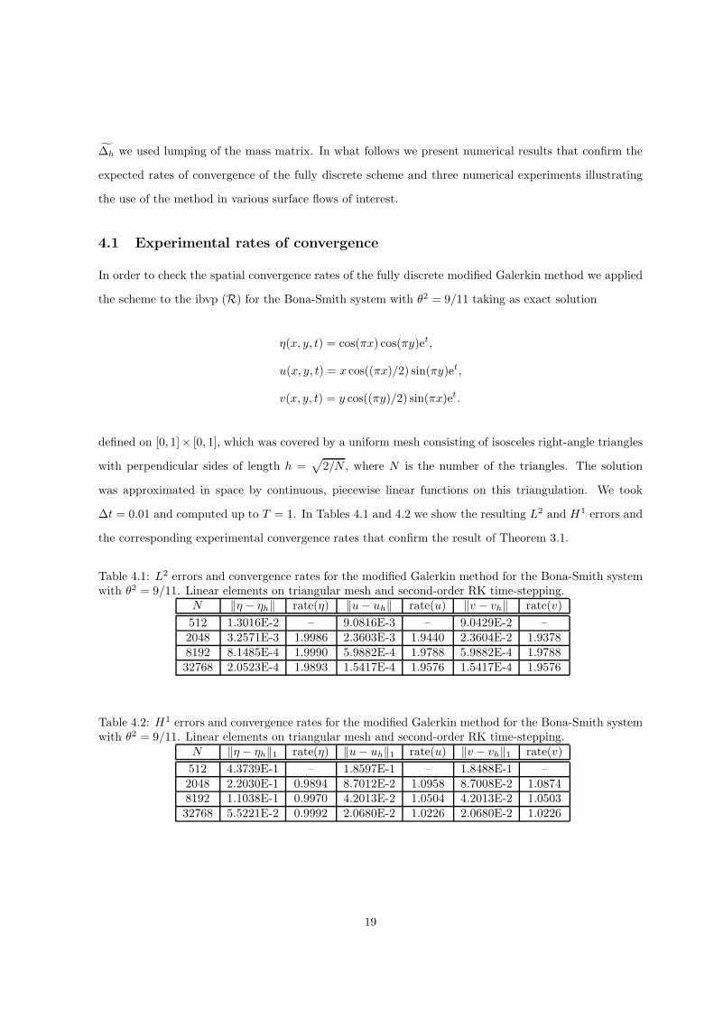
4.1 Experimental rates of convergence

In order to check the spatial convergence rates of the fully discrete modified Galerkin method we applied

the scheme to the ibvp (R) for the Bona-Smith system with θ2 = 9/11 taking as exact solution

η(x, y, t) = cos(πx) cos(πy)et,

u(x, y, t) = x cos((πx)/2) sin(πy)et,

v(x, y, t) = y cos((πy)/2) sin(πx)et.

defined on [0, 1]× [0, 1], which was covered by a uniform mesh consisting of isosceles right-angle triangles

with perpendicular sides of length h =√2/N , where N is the number of the triangles. The solution

was approximated in space by continuous, piecewise linear functions on this triangulation. We took

∆t = 0.01 and computed up to T = 1. In Tables 4.1 and 4.2 we show the resulting L2 and H1 errors and

the corresponding experimental convergence rates that confirm the result of Theorem 3.1.

Table 4.1: L2 errors and convergence rates for the modified Galerkin method for the Bona-Smith systemwith θ2 = 9/11. Linear elements on triangular mesh and second-order RK time-stepping.

N ‖η − ηh‖ rate(η) ‖u− uh‖ rate(u) ‖v − vh‖ rate(v)

512 1.3016E-2 – 9.0816E-3 – 9.0429E-2 –2048 3.2571E-3 1.9986 2.3603E-3 1.9440 2.3604E-2 1.93788192 8.1485E-4 1.9990 5.9882E-4 1.9788 5.9882E-4 1.978832768 2.0523E-4 1.9893 1.5417E-4 1.9576 1.5417E-4 1.9576

Table 4.2: H1 errors and convergence rates for the modified Galerkin method for the Bona-Smith systemwith θ2 = 9/11. Linear elements on triangular mesh and second-order RK time-stepping.

N ‖η − ηh‖1 rate(η) ‖u− uh‖1 rate(u) ‖v − vh‖1 rate(v)

512 4.3739E-1 – 1.8597E-1 – 1.8488E-1 –2048 2.2030E-1 0.9894 8.7012E-2 1.0958 8.7008E-2 1.08748192 1.1038E-1 0.9970 4.2013E-2 1.0504 4.2013E-2 1.050332768 5.5221E-2 0.9992 2.0680E-2 1.0226 2.0680E-2 1.0226

19

4.2 Solitary-wave-like pulse hitting a cylindrical obstacle

In our first experiment the domain that we consider is the rectangular channel [−15, 15]× [−30, 50] in

which is placed a vertical impenetrable cylinder centered at (0, 10) with radius equal to 1.5. We pose

normal reflective boundary conditions on the boundary of the cylinder and along the lines y = −30 and

y = 50, and homogeneous Neumann boundary conditions for η and v on the lateral boundaries x = ±15.

As initial conditions we use the functions

η0(x, y) = Asech2(

12

√3Acs(y + 10)

),

u0(x, y) = 0,

v0(x, y) = η0(x, y)−14η

20(x, y),

(4.32)

where A = 0.2 and cs = 1 + A2 , which represent a good approximation to a line solitary wave, [DMSI],

of the BBM-BBM system. We integrate under these initial and boundary conditions the Bona-Smith

system (1.1) with θ2 = 9/11 and compare its evolving solution with that of the BBM-BBM system, i.e.

(1.1) with θ2 = 2/3. The Bona-Smith system was discretized in space by the modified Galerkin method

(amended in a straightforward way to handle the Neumann conditions on v on the lateral boundaries)

with continuous, piecewise linear elements on a triangulation consisting of N = 290112 trangles; this

mesh was fine enough for the ‘convergence’ of the numerical solution. The same truangulation was used

to discretize in space the BBM-BBM system with the standard Galerkin method, [DMSI]. Both systems

were discretized in time with the improved Euler method with ∆t = 0.01.

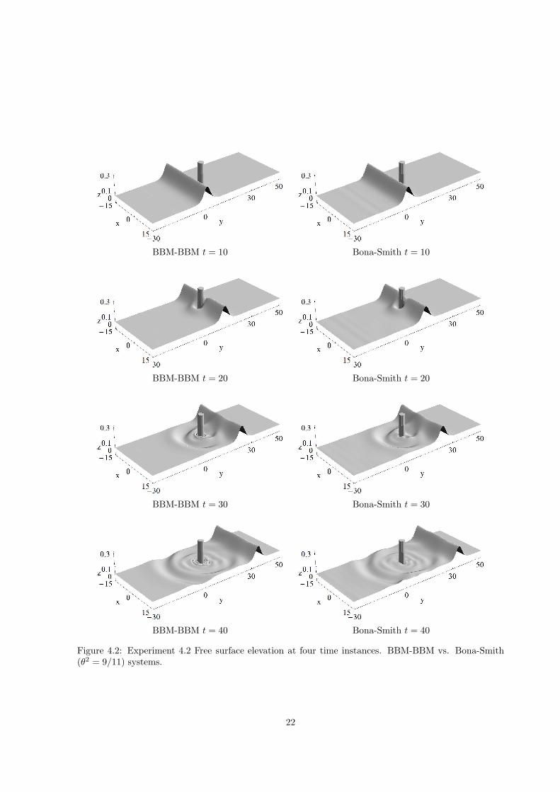
The line solitary-wave-like pulse is centered at y = −10 at t = 0. It propagates, mainly in the positive

y direction, travelling with a speed cs of about 1.05, cf. Figure 4.2. The bulk of the solitary wave travels

past the cylinder, while smaller amplitude scattered waves are produced by the interaction of the wave

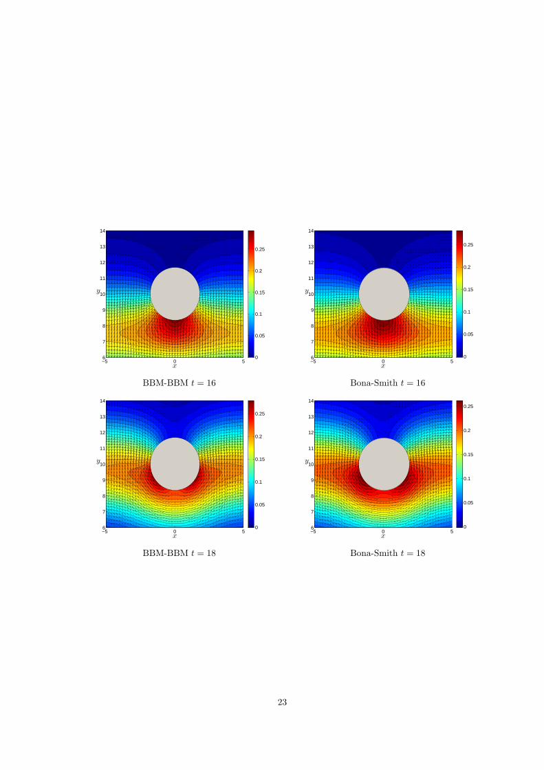
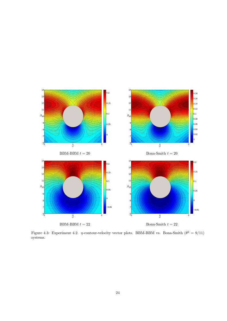
with the obstacle. Figure 4.3 shows, for both systems, contours of the elevation of the wave, superimposed

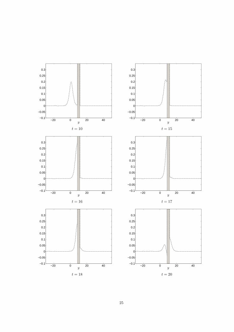
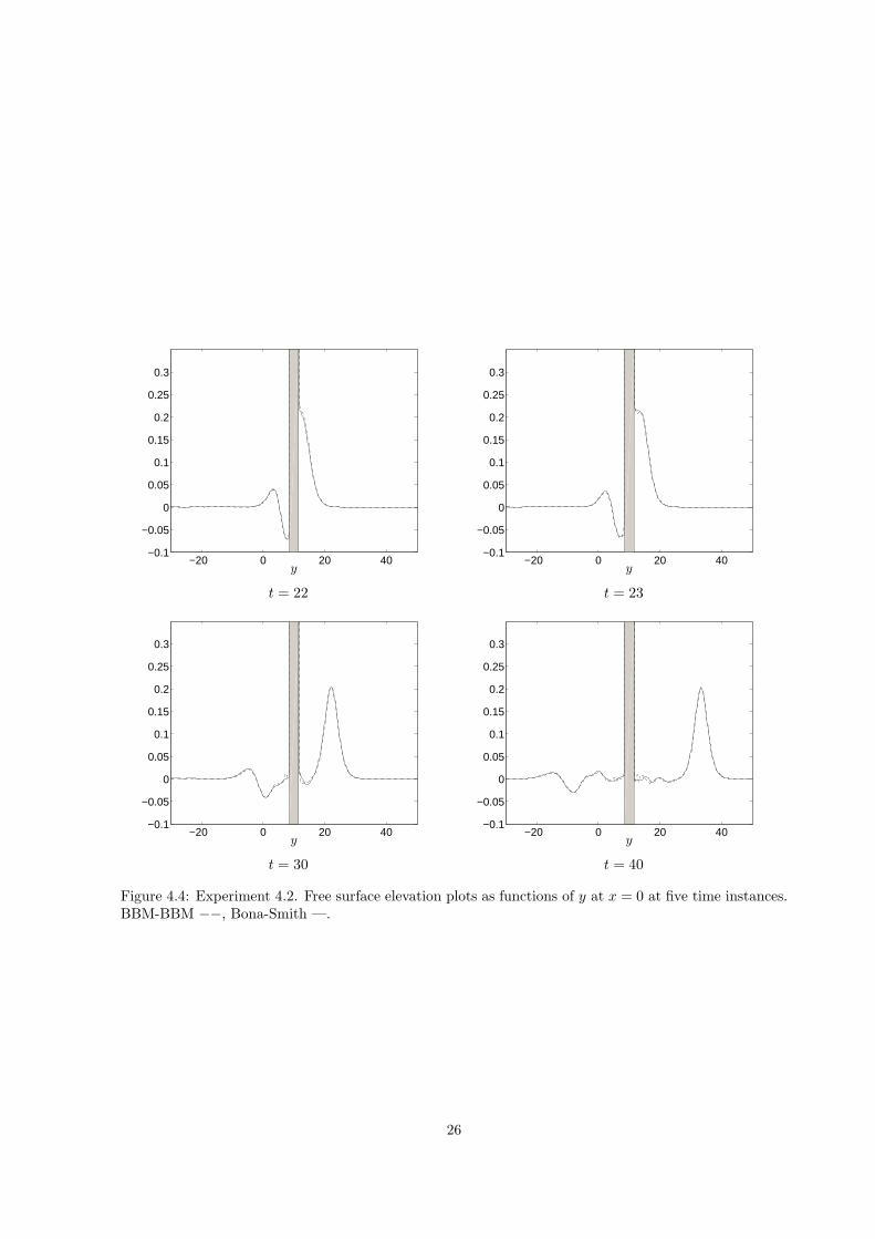
on velocity vector plots, near the obstacle during the passage of the solitary wave. Figure 4.4 shows the

free surface elevation for both systems as a function of y at x = 0 at several temporal instances. It

is worthwhile to note that the maximum run-up at the extreme upstream point (x, y) = (0, 8.5) of the

cylinder was equal to z = 0.335107 (achieved at t = 16.72) for the BBM-BBM system; the corresponding

run-up for the Bona-Smith system was z = 0.319960 at t = 16.74. The analogous values for the run-up on

the downstream point (0, 11.5) of the cylinder were z = 0.234310, t = 22.71 for the BBM-BBM system,

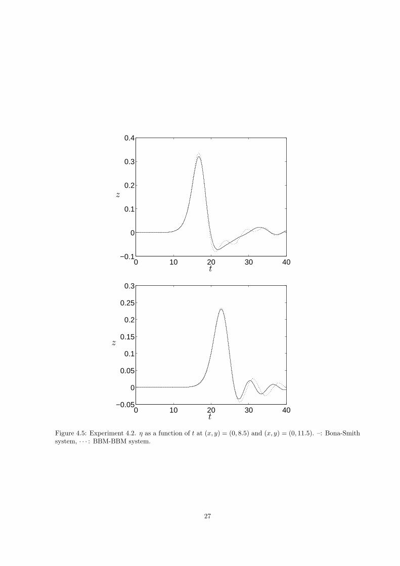
and z = 0.230590, t = 22.68 for the Bona-Smith system. Figure 4.5 shows the history of the free surface

elevation for both systems at the extreme points y = 8.5, y = 11.5 along the x = 0 diameter of the

20

cylinder, perpendicular to the impinging wave. In general, we did not observe great differences in the

behaviour of the solutions of the two systems.

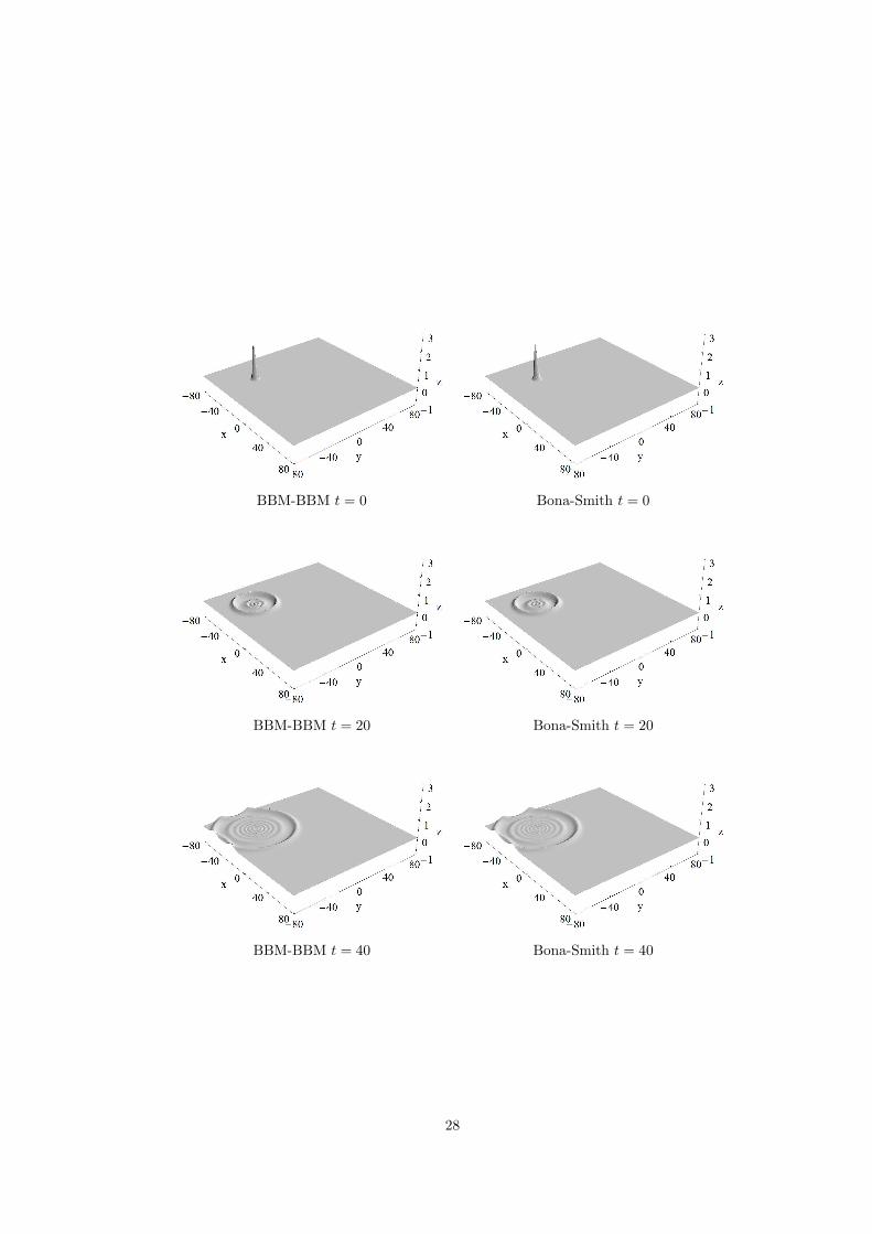
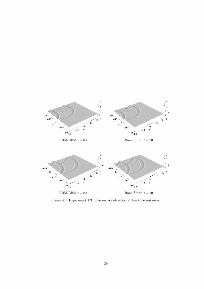
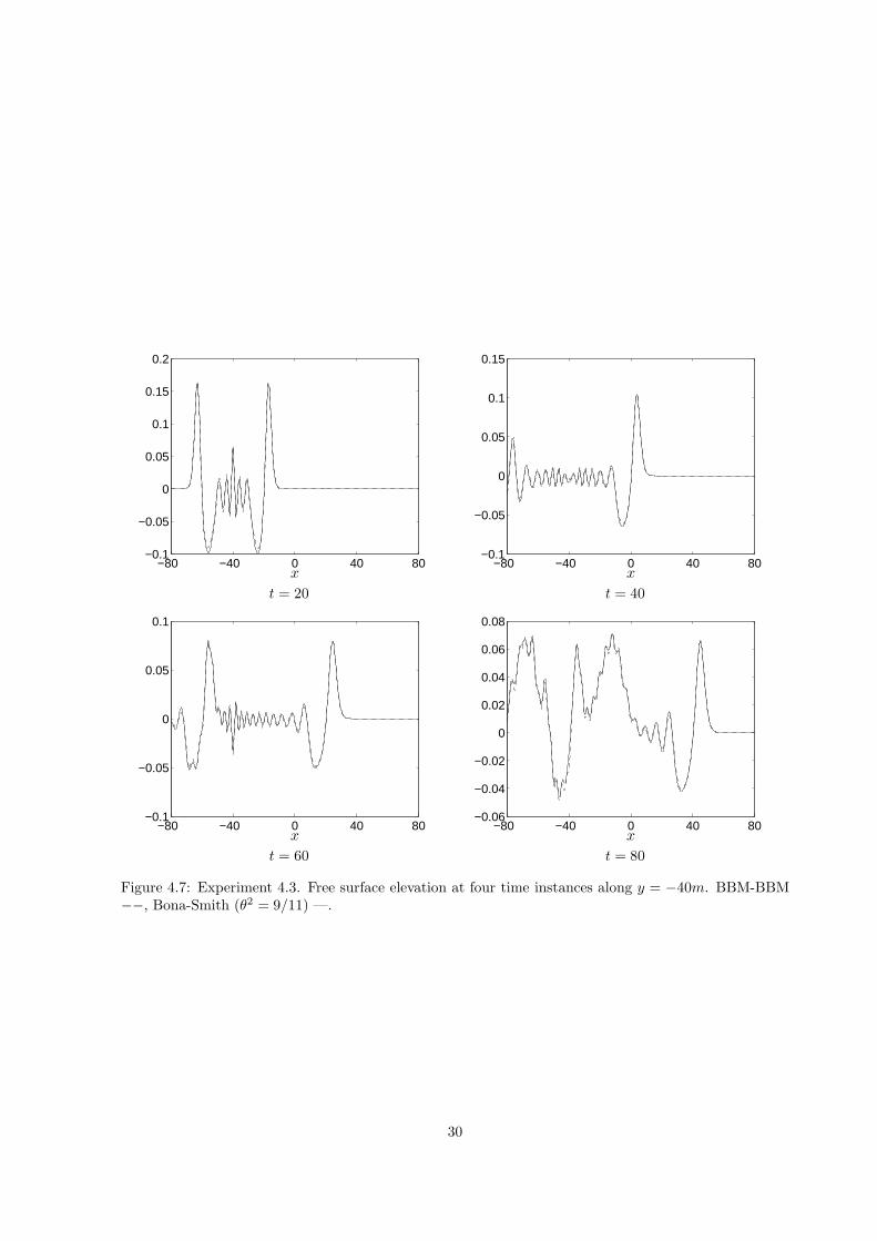
4.3 Evolution and reflection at the boundaries of a ‘heap’ of water

The sequence of plots of Figure 4.6 shows the temporal evolution of the free surface elevation of an initial

Gaussian ‘heap’ of water with

η0(x, y) = 2e−((x+40)2+(y+40)2)/5, v0(x, y) = 0,

as it collapses, forms radial outgoing riples and interacts with the reflective boundaries near a corner of

the square [−80, 80]× [−80, 80]. Again, no major differences were observed between the solutions of the

two systems (BBM-BBM and Bona-Smith, θ2 = 9/11). The computation was effected with N = 84992

triangular elements and ∆t = 0.1. Figure 4.7 shows the corresponding one-dimensional plots (along

x = −40) of the free surface elevation for both systems at four temporal instanses.

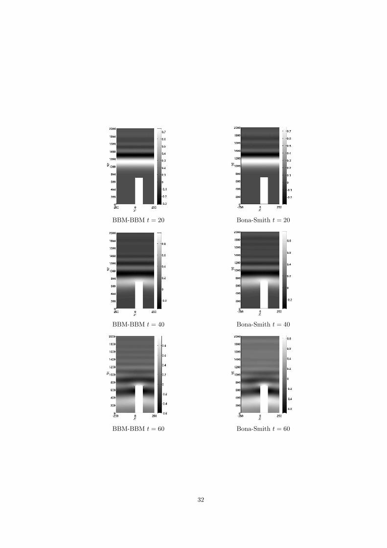
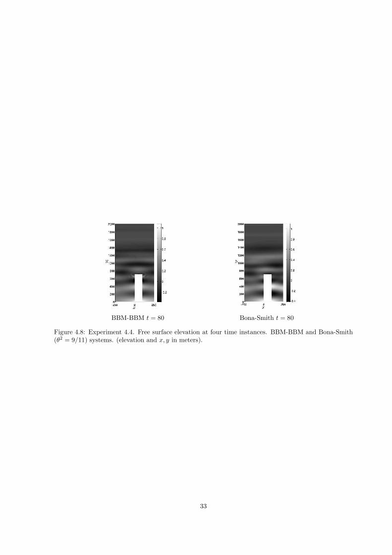
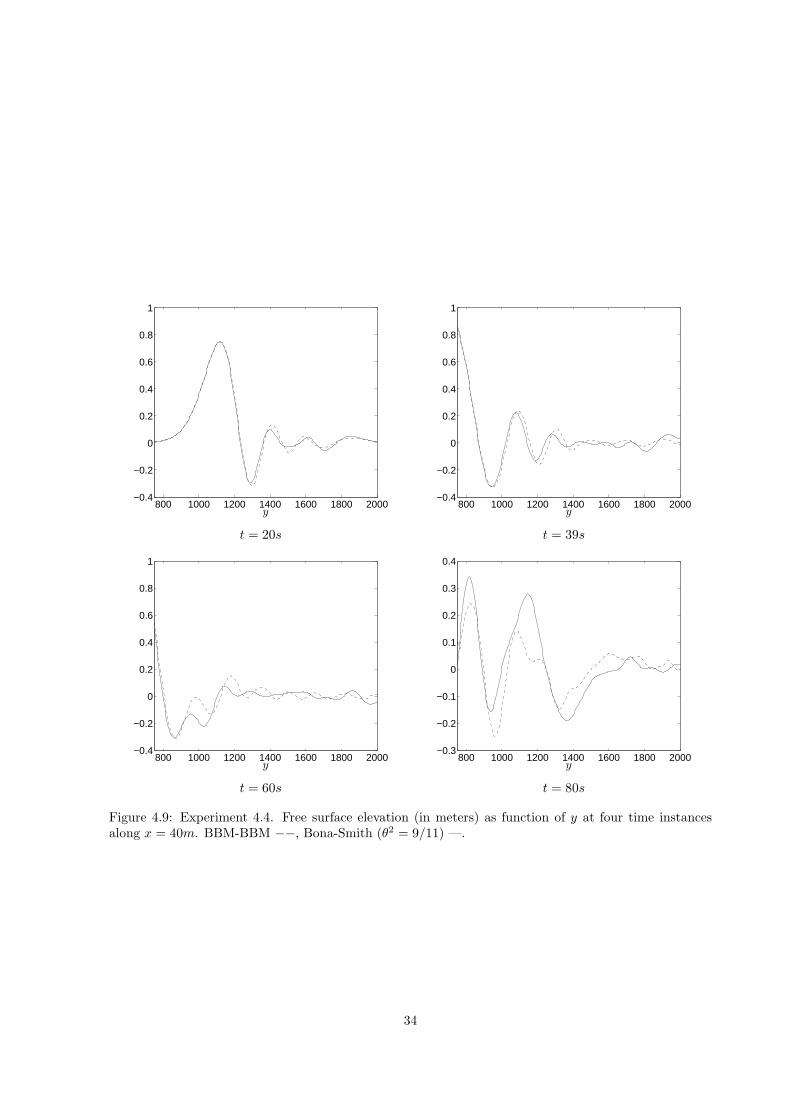
4.4 Line wave impinging on a ‘port’ structure

In this experiment we integrated the BBM-BBM and the Bona-Smith (θ2 = 9/11) systems in dimen-

sional variables. Our domain represents part of a ‘port’ of depth h0 = 50m consisting of the rectangle

[−250, 250]× [0, 2000] minus the rectangular ‘pier’ [0, 100]× [0, 700]. (All distances in meters). Normal

reflective boundary conditions are assumed to hold along the boundary of the pier and the intervals

[−250, 0] and [100, 250] of the x-axis, while homogeneous Neumann boundary conditions have been im-

posed on η and v on the remaining parts of the boundary. An initial wave with η0(x, y) = Ae−y−1500

6000 ,

A = 1m, and u0(x, y) = 0m/sec, v0(x, y) = − 12 (η0(x, y) −

14η

20(x, y))m/sec travels mainly towards the

negative y direction shedding a dispersive tail behind. (Both systems were integrated with N = 77632

triangles and ∆t = 0.01 sec). For the impinging wave at t = 30 sec we estimated that A/h0 ∼= 0.014,

λ/h0 ∼= 16.6, so that the Stokes number is approximately equal to 3.9, within the range of validity of

the Boussinesq systems. The incoming wave hits the pier and the port boundary at x = 0, is reflected

backwards and interacts with the remaining boundary. Figure 4.8 shows contour plots of the free surface

elevation for both systems at several temporal instances in the whole domain. In Figure 4.9 we plot the

computed free surface elevation as a function of y along the x = 40m line at several temporal instances

as the wave hits the pier front (y = 700) and reflects backwards. Most of the differences in the solution of

21

BBM-BBM t = 10 Bona-Smith t = 10

BBM-BBM t = 20 Bona-Smith t = 20

BBM-BBM t = 30 Bona-Smith t = 30

BBM-BBM t = 40 Bona-Smith t = 40

Figure 4.2: Experiment 4.2 Free surface elevation at four time instances. BBM-BBM vs. Bona-Smith(θ2 = 9/11) systems.

22

x

y

−5 0 56

7

8

9

10

11

12

13

14

0

0.05

0.1

0.15

0.2

0.25

x

y

−5 0 56

7

8

9

10

11

12

13

14

0

0.05

0.1

0.15

0.2

0.25

BBM-BBM t = 16 Bona-Smith t = 16

x

y

−5 0 56

7

8

9

10

11

12

13

14

0

0.05

0.1

0.15

0.2

0.25

x

y

−5 0 56

7

8

9

10

11

12

13

14

0

0.05

0.1

0.15

0.2

0.25

BBM-BBM t = 18 Bona-Smith t = 18

23

x

y

−5 0 56

7

8

9

10

11

12

13

14

0

0.05

0.1

0.15

0.2

x

y

−5 0 56

7

8

9

10

11

12

13

14

0

0.02

0.04

0.06

0.08

0.1

0.12

0.14

0.16

0.18

BBM-BBM t = 20 Bona-Smith t = 20

x

y

−5 0 56

7

8

9

10

11

12

13

14

−0.05

0

0.05

0.1

0.15

0.2

x

y

−5 0 56

7

8

9

10

11

12

13

14

−0.05

0

0.05

0.1

0.15

0.2

BBM-BBM t = 22 Bona-Smith t = 22

Figure 4.3: Experiment 4.2. η-contour-velocity vector plots. BBM-BBM vs. Bona-Smith (θ2 = 9/11)systems.

24

−20 0 20 40−0.1

−0.05

0

0.05

0.1

0.15

0.2

0.25

0.3

y−20 0 20 40

−0.1

−0.05

0

0.05

0.1

0.15

0.2

0.25

0.3

y

t = 10 t = 15

−20 0 20 40−0.1

−0.05

0

0.05

0.1

0.15

0.2

0.25

0.3

y−20 0 20 40

−0.1

−0.05

0

0.05

0.1

0.15

0.2

0.25

0.3

y

t = 16 t = 17

−20 0 20 40−0.1

−0.05

0

0.05

0.1

0.15

0.2

0.25

0.3

y−20 0 20 40

−0.1

−0.05

0

0.05

0.1

0.15

0.2

0.25

0.3

y

t = 18 t = 20

25

−20 0 20 40−0.1

−0.05

0

0.05

0.1

0.15

0.2

0.25

0.3

y−20 0 20 40

−0.1

−0.05

0

0.05

0.1

0.15

0.2

0.25

0.3

y

t = 22 t = 23

−20 0 20 40−0.1

−0.05

0

0.05

0.1

0.15

0.2

0.25

0.3

y−20 0 20 40

−0.1

−0.05

0

0.05

0.1

0.15

0.2

0.25

0.3

y

t = 30 t = 40

Figure 4.4: Experiment 4.2. Free surface elevation plots as functions of y at x = 0 at five time instances.BBM-BBM −−, Bona-Smith —.

26

0 10 20 30 40−0.1

0

0.1

0.2

0.3

0.4

t

z

0 10 20 30 40−0.05

0

0.05

0.1

0.15

0.2

0.25

0.3

t

z

Figure 4.5: Experiment 4.2. η as a function of t at (x, y) = (0, 8.5) and (x, y) = (0, 11.5). –: Bona-Smithsystem, · · · : BBM-BBM system.

27

BBM-BBM t = 0 Bona-Smith t = 0

BBM-BBM t = 20 Bona-Smith t = 20

BBM-BBM t = 40 Bona-Smith t = 40

28

BBM-BBM t = 60 Bona-Smith t = 60

BBM-BBM t = 80 Bona-Smith t = 80

Figure 4.6: Experiment 4.3. Free surface elevation at five time instances.

29

−80 −40 0 40 80−0.1

−0.05

0

0.05

0.1

0.15

0.2

x−80 −40 0 40 80

−0.1

−0.05

0

0.05

0.1

0.15

x

t = 20 t = 40

−80 −40 0 40 80−0.1

−0.05

0

0.05

0.1

x−80 −40 0 40 80

−0.06

−0.04

−0.02

0

0.02

0.04

0.06

0.08

x

t = 60 t = 80

Figure 4.7: Experiment 4.3. Free surface elevation at four time instances along y = −40m. BBM-BBM−−, Bona-Smith (θ2 = 9/11) —.

30

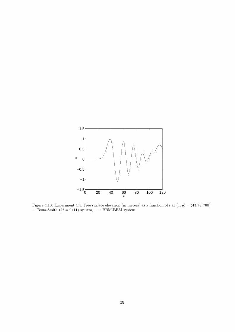
the two systems are of the order of 10 cm and are observed in the reflection phase. Figure 4.10 shows the

temporal history of the free surface elevation for both systems at the point (x, y) = (43.75, 700) at the

front of the pier. The maximum run-up observed at that point was equal to z = 0.976m (at t = 38.6 sec)

for the BBM-BBM system and to z = 0.988m (at t = 38.7) for the Bona-Smith system.

31

BBM-BBM t = 20 Bona-Smith t = 20

BBM-BBM t = 40 Bona-Smith t = 40

BBM-BBM t = 60 Bona-Smith t = 60

32

BBM-BBM t = 80 Bona-Smith t = 80

Figure 4.8: Experiment 4.4. Free surface elevation at four time instances. BBM-BBM and Bona-Smith(θ2 = 9/11) systems. (elevation and x, y in meters).

33

800 1000 1200 1400 1600 1800 2000−0.4

−0.2

0

0.2

0.4

0.6

0.8

1

y800 1000 1200 1400 1600 1800 2000

−0.4

−0.2

0

0.2

0.4

0.6

0.8

1

y

t = 20s t = 39s

800 1000 1200 1400 1600 1800 2000−0.4

−0.2

0

0.2

0.4

0.6

0.8

1

y800 1000 1200 1400 1600 1800 2000

−0.3

−0.2

−0.1

0

0.1

0.2

0.3

0.4

y

t = 60s t = 80s

Figure 4.9: Experiment 4.4. Free surface elevation (in meters) as function of y at four time instancesalong x = 40m. BBM-BBM −−, Bona-Smith (θ2 = 9/11) —.

34

0 20 40 60 80 100 120−1.5

−1

−0.5

0

0.5

1

1.5

t

z

Figure 4.10: Experiment 4.4. Free surface elevation (in meters) as a function of t at (x, y) = (43.75, 700).–: Bona-Smith (θ2 = 9/11) system, · · · : BBM-BBM system.

35

References

[ADMI] D. C. Antonopoulos, V. A. Dougalis and D. E. Mitsotakis, Initial-boundary-value problems for

the Bona-Smith family of Boussinesq systems, Adv. Differential Equations 14(2009), 27–53.

[ADMII] D. C. Antonopoulos, V. A. Dougalis and D. E. Mitsotakis, Numerical solution of Boussinesq

systems of the Bona-Smith type, (to appear in App. Num. Math.)

[BC] J. L. Bona and M. Chen, A Boussinesq system for two-way propagation of nonlinear dispersive

waves, Physica D 116(1998), 191–224.

[BCL] J. L. Bona, T. Colin, and D. Lannes, Long wave approximations for water waves, Arch. Rational

Mech. Anal. 178(2005), 373–410.

[BCSI] J. L. Bona, M. Chen and J.-C. Saut, Boussinesq equations and other systems for small-amplitude

long waves in nonlinear dispersive media: I. Derivation and Linear Theory, J. Nonlinear Sci.

12(2002), 283–318.

[BCSII] J. L. Bona, M. Chen and J.-C. Saut, Boussinesq equations and other systems for small-amplitude

long waves in nonlinear dispersive media: II. The nonlinear theory, Nonlinearity 17(2004), 925–952.

[BS] J. L. Bona and R. Smith, A model for the two-way propagation of water waves in a channel, Math.

Proc. Camb. Phil. Soc. 79(1976), 167–182.

[Ch] M. Chen, Numerical investigation of a two-dimensional Boussinesq system, Discrete Contin. Dyn.

Syst. 23(2009), 1169–1190.

[CI] M. Chen and G. Iooss, Periodic wave patterns of two-dimensional Boussinesq systems, European J.

of Mechanics B/ Fluids 25(2006),393–405.

[Ci] P. G. Ciarlet, The finite element method for elliptic problems, North-Holand, Amsterdam, New

York, Oxford, 1978.

[CT] M. Crouzeix and V. Thomee, The stability in Lp and W 1p of the L2-projection onto finite element

function spaces, Math. Comp. 48(1987), 521–532.

[DMSI] V. A. Dougalis, D. E. Mitsotakis and J.-C. Saut, On some Boussinesq systems in two space

dimensions: theory and numerical analysis, M2AN Math. Model. Numer. Anal. 41(2007), 825–854.

36

[DMSII] V. A. Dougalis, D. E. Mitsotakis and J.-C. Saut, On initial-boundary value problems for a

Boussinesq system of BBM-BBM type in a plane domain, Discrete Contin. Dyn. Syst. 23(2009),

1191–1204.

[RS] R. Rannacher and R. Scott, Some optimal error estimates for piecewise linear finite element ap-

proximations, Math. Comp., 38(1982), 437–445.

[SW] A. H. Schatz and L. B. Wahlbin, On the quasi-optimality in L∞ of the

H1-projection into finite

elements spaces, Math. Comp., 38(1982), 1–22.

[S] R. Scott, Optimal L∞ estimates for the finite element method on irregular meshes, Math. Comp.,

30(1976), 681–697.

37