Embed Size (px)
Citation preview
December 2006
NASA/TM–2006–214147
BOUSSOLE: A Joint CNRS-INSU, ESA, CNES, and NASA Ocean Color Calibration and Validation Activity
DavidAntoine,MalikChami,HervéClaustre,Fabriziod’Ortenzio,AndréMorel,GuislainBécu, BernardGentili,FrancisLouis,JoséphineRas,EmmanuelRoussier,AlecJ.Scott,DominiqueTailliez,StanfordB.Hooker,PierreGuevel,Jean-FrançoisDesté,CyrilDempsey,andDarrellAdams
https://ntrs.nasa.gov/search.jsp?R=20070028812 2019-02-16T11:47:10+00:00Z

The NASA STI Program Offi ce … in Profi le
Since its founding, NASA has been ded i cat ed to the ad vance ment of aeronautics and space science. The NASA Sci en tifi c and Technical Information (STI) Pro gram Offi ce plays a key part in helping NASA maintain this im por tant role.
The NASA STI Program Offi ce is operated by Langley Re search Center, the lead center for NASA s scientifi c and technical in for ma tion. The NASA STI Program Offi ce pro vides ac cess to the NASA STI Database, the largest col lec tion of aero nau ti cal and space science STI in the world. The Pro gram Offi ce is also NASA s in sti tu tion al mech a nism for dis sem i nat ing the results of its research and de vel op ment ac tiv i ties. These results are published by NASA in the NASA STI Report Series, which includes the following report types:
• TECHNICAL PUBLICATION. Reports of com plet ed research or a major signifi cant phase of research that present the results of NASA pro-grams and include ex ten sive data or the o ret i cal analysis. Includes com pi la tions of sig nifi cant scientifi c and technical data and in for ma tion deemed to be of con tinu ing ref er ence value. NASA s counterpart of peer-re viewed formal pro fes sion al papers but has less stringent lim i ta -tions on manuscript length and ex tent of graphic pre sen ta tions.
• TECHNICAL MEMORANDUM. Scientifi c and tech ni cal fi ndings that are pre lim i nary or of spe cial ized interest, e.g., quick re lease reports, working papers, and bib li og ra phies that contain minimal annotation. Does not contain extensive analysis.
• CONTRACTOR REPORT. Scientifi c and techni-cal fi ndings by NASA-sponsored con trac tors and grantees.
• CONFERENCE PUBLICATION. Collected pa pers from scientifi c and technical conferences, symposia, sem i nars, or other meet ings spon sored or co spon sored by NASA.
• SPECIAL PUBLICATION. Scientifi c, tech ni cal, or historical information from NASA pro grams, projects, and mission, often con cerned with sub-jects having sub stan tial public interest.
• TECHNICAL TRANSLATION. En glish-language trans la tions of foreign sci en tifi c and tech ni cal ma-terial pertinent to NASA s mis sion.
Specialized services that complement the STI Pro-gram Offi ceʼs diverse offerings include cre at ing custom the sau ri, building customized da ta bas es, organizing and pub lish ing research results . . . even pro vid ing videos.
For more information about the NASA STI Pro gram Offi ce, see the following:
• Access the NASA STI Program Home Page at http://www.sti.nasa.gov/STI-homepage.html
• E-mail your question via the Internet to [email protected]
• Fax your question to the NASA Access Help Desk at (301) 621-0134
• Telephone the NASA Access Help Desk at (301) 621-0390
• Write to: NASA Access Help Desk NASA Center for AeroSpace In for ma tion 7115 Standard Drive Hanover, MD 21076–1320
National Aeronautics and Space Administration
Goddard Space Flight CenterGreenbelt, Maryland 20771
December 2006
NASA/TM–2006–214147
BOUSSOLE: A Joint CNRS-INSU, ESA, CNES, and NASA Ocean Color Calibration and Validation Activity
DavidAntoine,MalikChami,HervéClaustre,Fabriziod’Ortenzio,AndréMorel,GuislainBécu, BernardGentili,FrancisLouis,JoséphineRas,EmmanuelRoussier,AlecJ.Scott,andDominiqueTailliez Laboratoired’OcéanographiedeVillefranche,Villefranche-sur-Mer,France
StanfordB.Hooker NASAGoddardSpaceFlightCenter,Greenbelt,Maryland
PierreGuevelandJean-FrançoisDesté ACRI-in,SophiaAntipolis,France
CyrilDempseyandDarrellAdams Satlantic,Inc.,Halifax,Canada

Available from:
NASA Center for AeroSpace Information National Technical Information Service7115 Standard Drive 5285 Port Royal RoadHanover, MD 21076-1320 Springfield, VA 22161
Antoine et al.
Preface
The Bouee pour l’acquisition de Series Optiques a Long Terme (BOUSSOLE) Project is a continuous ac-tivity, which evolves over time to deal with the multitude of activities associated with long-term oceanic
deployments. This report is to be seen as a snapshot of the present state of the activity and achievements1.An overview of the different technical aspects is provided; it is out of the scope of this report to provide alldetails of all activities. It is directed at providing basic information that is needed for an overall understandingof what has been done and what is presently being done in all segments of the project. More detailed analysesof specific technical aspects of the project will be the subject of other, more detailed, reports. BOUSSOLE is ajoint effort involving multiple organizations, which are combining the work of a lot of people, and is funded andsupported by the following agencies and academic or governmental institutes:
• Centre National de la Recherche Scientifique2 (CNRS),• Institut National des Sciences de l’Univers3 (INSU),• European Space Agency (ESA),• Centre National d’Etudes Spatiales4 (CNES),• National Aeronautics and Space Administration (NASA),• Universite Pierre et Marie Curie5 (UPMC), and• Observatoire Oceanologique de Villefranche-sur-Mer6.
The resources these organizations have provided were critical in establishing BOUSSOLE as a field site forocean color calibration and validation activities, but they were not the only ones who needed to cooperate.Indeed, a very important participant was never consulted, but luckily, decided to send a representative anyway.Before entering into the details of this technical report, it seems appropriate to add this silent partner to theintroductions provided here, particularly because the task for this recently hired team member is to remain onsite day and night to survey the mooring and provide daily status reports. After this page is turned, hopefullythe revulsion of isolating a team member in the unforgiving environment of the open sea will be replaced with anappreciation for the beauty of submarine life and the largely unseen world oceanographers strive to understand.Incidentally, this is also recognition of the vital and hard work the technical staff associated with BOUSSOLEare continuously doing at sea. And, who knows, maybe you will meet this new staff member the next timeyou are at sea. This might very well reassure you—a scientist or engineer inevitably focused too much on theproblem at hand (our common fate)—that you still possess an open mind capable of seeing what is happeningaround you and being pleasantly surprised by what is revealed as the layers of a problem are peeled away . . .
1 Additional details are available on the BOUSSOLE Web site http://www.obs-vlfr.fr/Boussole.2 National Center for Scientific Research3 National Institute for Science of the Universe4 National Center for Space Studies5 University of Pierre and Marie Curie6 Oceanographic Observatory of Villefranche
iii

BOUSSOLE: A Joint CNRS-INSU, ESA, CNES, and NASA Ocean Color Calibration and Validation Activity
This is the regalec, or as it is also known, the oarfish, kingof the herring, or ribbonfish (actually Regalecus glesne).The oarfish is a widely-distributed marine fish having aslender silvery body up to 11 m (36 ft) in length, a dor-sal fin running the entire length of the body with red-tipped anterior rays rising above the head, and ventralfins reduced to long filaments. It swims by rhythmicallyundulating the dorsal fin (a motion resembling that of asnake), while keeping the body itself straight. It’s largesize and snake-like appearance is believed to be the sourceof ancient mariner tales of sea serpents. The specimen—or rather, team member—shown here is about 4 m long.The oarfish is rarely observed in situ, but this one exhibitsa keen interest in the status of the BOUSSOLE buoy.
Note also the clarity of the seawater at the BOUSSOLEsite. The details of the in-water superstructure and oneof the support arms where the in-water instruments aremounted (Sect. 5.2) are clearly visible in the top-left pic-ture, whereas in the bottom-right picture, two of thedivers in their small service boat and the above-water partof the upper superstructure are easily discerned. Oarfish,like this one, have been observed swimming in a verti-cal orientation, with their long axis perpendicular to theocean surface. In this posture, the downstreaming lightsilhouettes prey, making them easier to spot.
Photographs: David Luquet, ObservatoireOceanologique de Villefranche-sur-Mer
iv
Antoine et al.
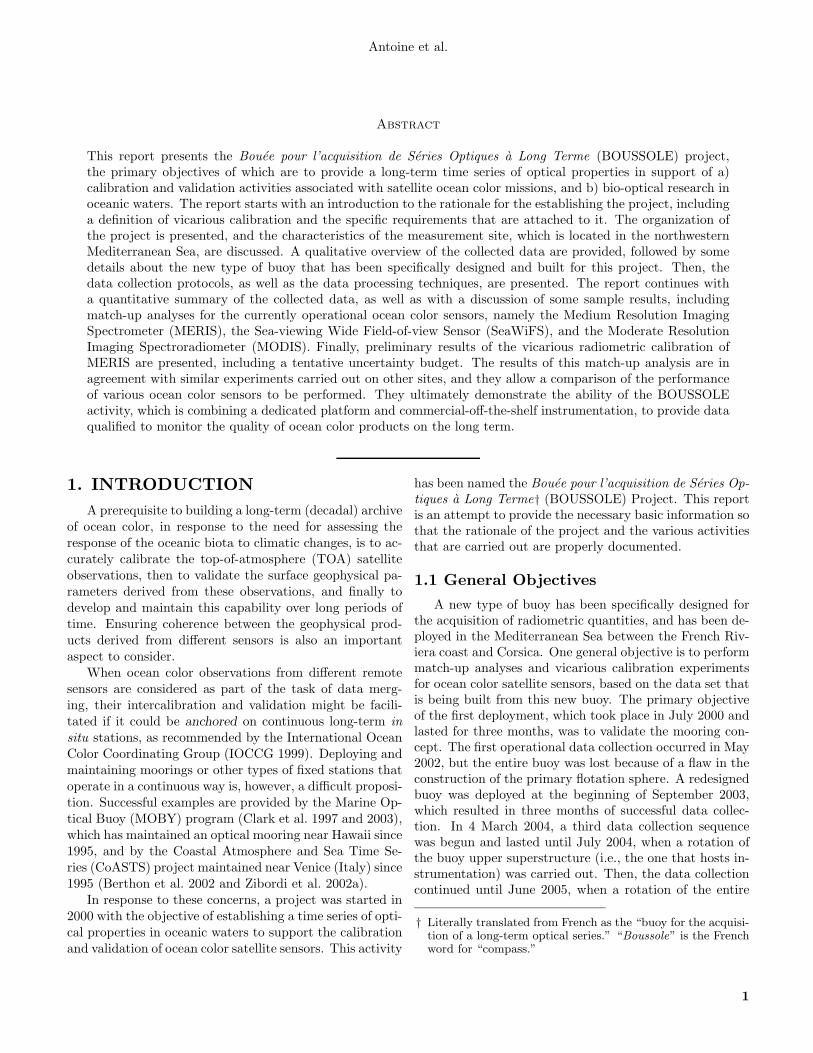
Abstract
This report presents the Bouee pour l’acquisition de Series Optiques a Long Terme (BOUSSOLE) project,the primary objectives of which are to provide a long-term time series of optical properties in support of a)calibration and validation activities associated with satellite ocean color missions, and b) bio-optical research inoceanic waters. The report starts with an introduction to the rationale for the establishing the project, includinga definition of vicarious calibration and the specific requirements that are attached to it. The organization ofthe project is presented, and the characteristics of the measurement site, which is located in the northwesternMediterranean Sea, are discussed. A qualitative overview of the collected data are provided, followed by somedetails about the new type of buoy that has been specifically designed and built for this project. Then, thedata collection protocols, as well as the data processing techniques, are presented. The report continues witha quantitative summary of the collected data, as well as with a discussion of some sample results, includingmatch-up analyses for the currently operational ocean color sensors, namely the Medium Resolution ImagingSpectrometer (MERIS), the Sea-viewing Wide Field-of-view Sensor (SeaWiFS), and the Moderate ResolutionImaging Spectroradiometer (MODIS). Finally, preliminary results of the vicarious radiometric calibration ofMERIS are presented, including a tentative uncertainty budget. The results of this match-up analysis are inagreement with similar experiments carried out on other sites, and they allow a comparison of the performanceof various ocean color sensors to be performed. They ultimately demonstrate the ability of the BOUSSOLEactivity, which is combining a dedicated platform and commercial-off-the-shelf instrumentation, to provide dataqualified to monitor the quality of ocean color products on the long term.
1. INTRODUCTIONA prerequisite to building a long-term (decadal) archive
of ocean color, in response to the need for assessing theresponse of the oceanic biota to climatic changes, is to ac-curately calibrate the top-of-atmosphere (TOA) satelliteobservations, then to validate the surface geophysical pa-rameters derived from these observations, and finally todevelop and maintain this capability over long periods oftime. Ensuring coherence between the geophysical prod-ucts derived from different sensors is also an importantaspect to consider.
When ocean color observations from different remotesensors are considered as part of the task of data merg-ing, their intercalibration and validation might be facili-tated if it could be anchored on continuous long-term insitu stations, as recommended by the International OceanColor Coordinating Group (IOCCG 1999). Deploying andmaintaining moorings or other types of fixed stations thatoperate in a continuous way is, however, a difficult proposi-tion. Successful examples are provided by the Marine Op-tical Buoy (MOBY) program (Clark et al. 1997 and 2003),which has maintained an optical mooring near Hawaii since1995, and by the Coastal Atmosphere and Sea Time Se-ries (CoASTS) project maintained near Venice (Italy) since1995 (Berthon et al. 2002 and Zibordi et al. 2002a).
In response to these concerns, a project was started in2000 with the objective of establishing a time series of opti-cal properties in oceanic waters to support the calibrationand validation of ocean color satellite sensors. This activity
has been named the Bouee pour l’acquisition de Series Op-tiques a Long Terme† (BOUSSOLE) Project. This reportis an attempt to provide the necessary basic information sothat the rationale of the project and the various activitiesthat are carried out are properly documented.
1.1 General ObjectivesA new type of buoy has been specifically designed for
the acquisition of radiometric quantities, and has been de-ployed in the Mediterranean Sea between the French Riv-iera coast and Corsica. One general objective is to performmatch-up analyses and vicarious calibration experimentsfor ocean color satellite sensors, based on the data set thatis being built from this new buoy. The primary objectiveof the first deployment, which took place in July 2000 andlasted for three months, was to validate the mooring con-cept. The first operational data collection occurred in May2002, but the entire buoy was lost because of a flaw in theconstruction of the primary flotation sphere. A redesignedbuoy was deployed at the beginning of September 2003,which resulted in three months of successful data collec-tion. In 4 March 2004, a third data collection sequencewas begun and lasted until July 2004, when a rotation ofthe buoy upper superstructure (i.e., the one that hosts in-strumentation) was carried out. Then, the data collectioncontinued until June 2005, when a rotation of the entire
† Literally translated from French as the “buoy for the acquisi-tion of a long-term optical series.” “Boussole” is the Frenchword for “compass.”
1
BOUSSOLE: A Joint CNRS-INSU, ESA, CNES, and NASA Ocean Color Calibration and Validation Activity
buoy and mooring line was accomplished. This was actu-ally the beginning of a nearly uninterrupted succession ofdeployments.
Another objective of the BOUSSOLE activity is to per-form vicarious calibration experiments. They should al-low the TOA radiance to be simulated and compared tothe satellite measurements, in particular for the EuropeanMedium Resolution Imaging Spectrometer (MERIS) sen-sor (Rast et al. 1999). In this way, the need for a changein the preflight calibration coefficients for a given sen-sor might be evaluated, and its amount quantified. Fromthis data set, match-up analyses shall be also possible forchlorophyll a (Chl a) concentration and water-leaving radi-ances, as well as algorithm evaluation (atmospheric correc-tion and pigment retrieval). Because of a certain common-ality in the band sets of the new generation of ocean colorsensors, the data acquired with the buoy might be used forseveral of these sensors, and then contribute to the interna-tional effort of intercalibrating them and of cross-validatingtheir products, which were amongst the basic goals of theSensor Intercomparison for Marine Biological and Inter-disciplinary Ocean Studies (SIMBIOS) project (McClain1998). In addition, some protocol issues (measurements)are specifically linked to the use of buoys, while others, ofgeneral concern to marine optics measurements, may findspecific answers when buoys are used. These aspects areexamined, which, to the best of the project knowledge,have not been thoroughly investigated up to now.
In parallel to these operational objectives (i.e., the cal-ibration and validation activities), the assembled data setwill be used for more fundamental studies in marine op-tics and bio-optics. Among the questions and topics thatmight be addressed are the diurnal cycles of optical proper-ties, the response to abrupt environmental changes (stormsand so-called red rain events), the relationships betweenchlorophyll concentration and the inherent optical proper-ties, the role of a fluctuating interface in establishing theradiative regime, the bidirectionality of the radiance field,the annual cycles and interannual variations of the opti-cal properties, the use of these properties as indicators ofother biogeochemical properties, and the interpretation ofthe natural fluorescence signal.
1.2 Vicarious CalibrationThe need to vicariously calibrate an ocean color satel-
lite sensor was first demonstrated for the Coastal ZoneColor Scanner (CZCS), which was a proof-of-concept mis-sion with an operational capability spanning 1979–1986.On one hand, this instrument was not equipped with thenecessary onboard devices for the monitoring of the long-term degradation of the instrument response sensitivity(internal lamps suffered a rapid degradation), and, on theother hand, the mission did not include an extensive vi-carious calibration program. In the end, the calibration ofthe CZCS was never based on a robust scientific capabilityand has never been sufficiently confirmed.
The converse situation is illustrated by the Sea-viewingWide Field-of-view Sensor (SeaWiFS) mission (Hooker etal. 1992). The instrument is equipped with a solar dif-fuser and has the capability of viewing the full moon, bothof which are used to track the temporal stability of theinstrument; and, in addition, an extensive vicarious cali-bration and algorithm validation program was set up priorto launch (McClain et al. 1992). The vicarious calibrationportion of the latter is based on the deployment of a perma-nent optical buoy, the MOBY program (Clark et al. 1997),which is moored in Case-1 waters near the island of Lanaiin Hawaii. In parallel to this central and key element, ex-tensive campaigns are conducted around the world ocean,in order to collect radiometric measurements and ancillarydata in a variety of environments (e.g., Robins et al. 1996,Aiken et al. 1998, and Barlow et al. 2003). These dataare used to permanently evaluate the quality of the level -2products and improve, whenever possible, the applicablebio-optical algorithms.
Without ground-truth data—more properly sea-truthdata—it is impossible to maintain the calibration of a satel-lite sensor at the desired level over the full course of themission, which is generally designed to be on the orderof about five years (although many satellites operate forlonger periods of time as evidenced by SeaWiFS, whichwas launched in 1997). This is not caused by any weak-ness in the sensor nor in the onboard calibration devices; itis simply because of unavoidable physical considerations:the goal of modern ocean color sensors is to provide thewater-leaving radiance in the blue with a 5% accuracy overoligotrophic, chlorophyll-depleted, waters (Gordon 1997),which can be expressed as well as an uncertainty of 0.002in terms of reflectance (Antoine and Morel 1999). Becausethis marine signal only represents about 10% (at most) ofthe TOA radiance (i.e., the radiance directly measured bythe spaceborne sensor), achieving this goal requires the in-struments involved are calibrated to better than 0.5%, orapproximately 1%. This is extremely challenging consid-ering the present technology, and probably will remain anelusive accomplishment.
A successful strategy for ensuring high-quality obser-vations from an ocean color satellite mission is based on arather pragmatic approach and consists of a) making thebest possible effort when initially characterizing and cali-brating the spaceborne instrument on the ground, b) usingonboard calibration devices or maneuvers to track sensi-tivity changes over time while on orbit, and c) adjustingindividual channels to force agreement with the sea-truthdata—the basis of the vicarious calibration procedure—which produces a final adjustment for the whole (instru-ment plus algorithms) system.
1.3 Moorings as Long-Term Data Sources
Maintaining a permanent optical mooring is a costly,but pertinent, solution to the problem of how best to col-
2
Antoine et al.
lect a significant number of the needed sea-truth obser-vations for the vicarious calibration process. This is eas-ily demonstrated by comparing this option to the usualoceanographic practice of deploying research vessels to var-ious parts of the world ocean.
Past experience has demonstrated that a one-monthcruise is able to produce a maximum of a dozen of match-up points when conditions are extremely favorable. This issimply because of the number of conditions that must besimultaneously fulfilled for a measurement to be usable forthe calibration and validation process (clear sky, low windspeed, acquisition within a maximum of 1 h of satellite overpass, nominal operation of the instruments, etc.).
A permanent mooring is well adapted to maintaininga consistent time series of in situ measurements over along period of time, because the needed personnel, equip-ment, and methodologies remain mostly fixed once theyare established. Although the latter is a demonstrable ad-vantage, ensuring the same level of consistency betweenthe people, equipment, and protocols from different cruisesinevitably adds some extra uncertainties in the overall en-terprise of data collection and processing. A permanentstation is also well suited for developing and testing new in-strumentation as well as new algorithms, and therefore, topermanently improve the quality and the variety of prod-ucts that can be derived from the ocean color observationsat the TOA level. It is also a unique opportunity to es-tablish the cross calibration between different sensors byanchoring them to the same in situ time series.
A criticism that is often made of the mooring optionis the uniqueness of the measurement site. This is actu-ally not an argument, because the vicarious calibrationprocess is a physical process, which does not require thatdata from a variety of different environments are collected.It requests, however, that the maximum of information(quantitatively as well as qualitatively) are collected atthe selected site so that the reconstruction of the TOAsignal through radiative transfer calculations is performedwith the best possible accuracy. This does not preclude,however, that data are collected in other environments forvalidation of level-2 products and for verification of thecalibration obtained at the initial mooring site.
The scheme briefly exposed above (i.e., a permanentcalibration site and a parallel program of validation fromships) was adopted by the SeaWiFS Project. It has beena success, and this sensor is probably the best-calibratedocean color sensor the community has ever had, at leastuntil next-generation sensors such as MERIS and MODISare operational over a similar time span and demonstratetheir full potential.
1.4 Specific Protocol Requirements
It has just been said that moorings are adapted to pro-vide large numbers of in situ data points, however, whatwould be the advantage in case these data are not of the
desired quality? The question arises, because the measure-ment conditions on a mooring may degrade the final qual-ity of the data. Buoys are often moving a lot, because thesea is rarely totally flat, so the instruments are (at somelevel) in an unstable situation. They are often made ofa large floating body with the equipment installed under-neath, so the light sensors can be significantly shaded. Theprolonged immersion of the instruments is favorable to thedevelopment of biofouling. Finally, the number of calibra-tions that can be performed, which is particularly impor-tant to track the temporal stability of the radiometers, isdependent on the frequency of maintenance visits (duringwhich instruments can be exchanged). The servicing in-terval might be insufficient in some cases, either because itis inherent to the project organization or because of severeweather. Consequently, the qualification of a given moor-ing program with respect to the ocean color calibration andvalidation requirements should consider the above pointsand evaluate whether or not they have been accounted forthrough a protocol. The data collected by the moored in-struments should be, for instance, compared to the samedata derived from ship-deployed instrumentation.
2. STRATEGYThe BOUSSOLE Project is composed of three basic
and complementary elements: a) a monthly cruise pro-gram, b) a permanent optics mooring, and c) a coastalAerosol Robotic Network (AERONET) station. Each ofthese three segments is designed to provide specific mea-surements of various parameters at different and comple-mentary spatial and temporal scales. When combined,they provide a comprehensive time series of near-surface(0–200 m) oceanic and atmospheric inherent optical prop-erties (IOPs) and apparent optical properties (AOPs), re-quired to accomplish several objectives:
• Performing the vicarious radiometric calibration ofsatellite ocean color sensors (i.e., the simulation ofthe TOA radiances recorded by the sensor in var-ious spectral bands, including the visible and nearinfrared (NIR) domains);
• Performing the validation of the level-2 geophysi-cal products that are produced from the observa-tions of these satellite ocean color sensors, includ-ing the normalized water-leaving radiances, the pig-ment concentrations, and the aerosol optical thick-ness (AOT) and types;
• Performing both of these operations on a long-termbasis (i.e., at least for the duration of the MERISmission, for which the BOUSSOLE project has beenprimarily set up); and
• Making progress in several domains of ocean opticsand bio-optics, as already stated earlier (Sect. 1).
A basic description of the three elements and the opera-tions carried out there is given below.
3
BOUSSOLE: A Joint CNRS-INSU, ESA, CNES, and NASA Ocean Color Calibration and Validation Activity
2.1 Monthly Maintenance Cruises
From July 2001 to December 2003, the BOUSSOLEoptics cruises were planned with a duration of three con-secutive days distributed on a near-monthly basis withinthe budget of 30–31 sea days per year aboard the researchvessel (R/V) Tethys II. In these first two and a half years,some cruises were unsuccessful in data collection because ofbad weather preventing ship departure or scientific workfor the entire three days. For this reason, for 2004 thecruise duration during the seasons with characteristicallyunsettled conditions, October to April, were increased toup to five days with a subsequent reduction in the over-all number of cruises per year. The same logic is followedsince 2005, yet without reduction of the number of cruises(i.e., 12 cruises per year).
The so-called optics day (defined as the period dur-ing which the Sun is at an angle greater than 20◦ abovethe horizon) commences and ends with a 400 m conduc-tivity, temperature, and depth (CTD) profile. The CTDsensors are mounted on a rosette equipped with 11 Niskinbottles. Spectral absorption and attenuation, a(z, λ) andc(z, λ), respectively (z indicates depth and λ denotes wave-length), is measured at nine wavelengths using a West-ern Environmental Technology Laboratories (WETLabs),Inc. (Philomath, Oregon) 25 cm pathlength AC-9 with en-hanced data handling (AC-9+) mounted in the twelfth bot-tle position. Additional sensors are the CTD and O2 sen-sors, a colored dissolved organic matter (CDOM) fluorom-eter, a chlorophyll fluorometer, and a backscattering (bb)sensor (Sect. 6.2).
For at least one CTD cast each day, the bottles arefired at selected depths during the ascent of the CTD overthe 0–400 m depth range. The collection depths are de-cided during the descent of the CTD after observation ofthe fluorescence profile, thus optimizing the representationof any features in the water column. For other casts, trip-licate samples are collected from 5 and 10 m. In the sum-mer, when the optics day is longer or when there are idealsatellite match-up conditions, an additional CTD profile isperformed around solar noon or in time with a SeaWiFSor MODIS overpass.
Seawater samples (2.8 L) are filtered through What-man GF/F filters using a low pressure vacuum and storedin liquid nitrogen. Back in the laboratory, the filters arelater analyzed by high performance liquid chromatography(HPLC) and spectrophotometry for pigments and partic-ulate absorption, respectively (Sect. 7.1 and 7.2).
Multispectral upward and downward irradiance pro-files, Eu(z, λ) and Ed(z, λ), respectively, are performedwith the objectives of providing synchronous in situ Sea-WiFS and MERIS calibration and validation profiles, char-acterizing the light field throughout the day at the BOUS-SOLE site, and providing a support data set for observa-tions from the BOUSSOLE buoy. During these profilingsessions, multiple profiles are performed with a SeaWiFS
Profiling Multichannel Radiometer (SPMR), if possible, toimprove the quality of the data by replicates. The firstSPMR session of the day begins after the first CTD pro-file, and continues ideally until the end of the optics day,before the final CTD profile. A gimbaled 4π photosynthet-ically available radiation (PAR) sensor positioned on theforedeck and operated from the CTD computer serves asa light field stability indicator during SPMR profiling.
For the satellite passes, whenever possible, SPMR pro-filing is performed within 1 h of satellite overhead passesof SeaWiFS and MERIS and around solar noon. Optimalconditions for these measurements are low humidity, blueskies and flat, calm sea surface. If the sky is clear and seaconditions are calm, a second-generation Satellite Valida-tion for Marine Biology and Aerosol Determination (SIM-BADA) measurements are performed consecutively wherepossible with SPMR profiles (only carried out from July2001 to July 2003). If sea conditions are poor but the sun isclear of clouds, SIMBADA sun photometer measurementscan be made at intervals throughout the day to measureatmospheric optical thickness.
When sea surface conditions are calm, a low-volume(small shadow) surface float is used to suspend the SPMRin a vertical position with the Eu sensor submerged ap-proximately 20 cm below the surface. The SPMR is heldin this orientation for a duration of at least 3 min and isreleased when the light field is expected to be stable. Thisdecision is a judgement call based on sky observation andmonitoring of the PAR sensor. To start the descent, anelectronic trigger mechanism is fitted to the surface float,which can be controlled from inside the lab. Multiple de-scents ideally will be started in this way and the data willbe used to assess near-surface upwelled radiance (Lu) ex-trapolation model calculations.
For each cruise, at the end of the on-site optics mea-surements, there is a CTD and IOP transect between theBOUSSOLE site and the port of Nice (France) consistingof six fixed locations. The aim is to have a representativeprofile of the water column on either side of the bound-ary to the Ligurian Current. The approximate time ofday that this transect is performed is kept similar for eachcruise, whenever possible, to minimize the influence of di-urnal variability.
A study of the spatial variability at the BOUSSOLEsite was performed once on each cruise until the middleof 2005. A fixed square mile quadrilateral grid based onGlobal Positioning System (GPS) data is covered by theship at a speed of 7–8 kts. During transit around this grid,water is continuously being pumped from an inlet beneaththe ship’s hull, and directed to the thermosalinograph anda fluorometer. Samples are collected at three equidistantpoints along this grid, for subsequent HPLC analyses, inorder to convert dimensionless fluorescence measurementsinto chlorophyll concentrations.
On other uninterrupted transits between Nice and theBOUSSOLE site, particularly when there is a high sun an-gle and clear skies, CIMEL Electronique (Paris, France)
4

LigurianCurrentNice
LigurianSea
St. 6
St. 5
St. 4
St. 3
St. 2
St. 1DYFAMED
Site
BOUSSOLESite
Meteo Buoy
43° 42' N
43° 36' N
43° 30' N
43° 24' N
43° 18' N7° 54' E7° 42' E7° 30' E7° 18' E9° E8° E7° E
44° N
43° N
42° N
a b
Antoine et al.
Fig. 1. The coastal area of the northwestern part of the Mediterranean Sea showing a) the southern coastof France and the island of Corsica, plus the generalized work area in the Ligurian Sea (black star) for theBOUSSOLE activity; and b) a magnification showing the position of the BOUSSOLE mooring plus theDynamique des Flux Atmospheriques en Mediterranee (DYFAMED) site and the Meteo buoy maintained bythe French weather forecasting agency (Meteo France). The positions of the six stations, which are sampledonce a month during transits from Nice to the BOUSSOLE site, are also displayed.
model 317 (CE-317) sun photometer measurements aretaken at 30 min intervals (approximately 5 nmi) to charac-terize the variability in atmospheric optical thickness be-tween the Cap Ferrat sun photometer site and the BOUS-SOLE site.
2.2 The Mooring Site
The mooring site is equipped with a new type of buoy,specifically designed for collecting optical data (Sect. 5)with two specific objectives: a) obtain a near-continuoussampling at the surface (depths less than 10 m), in orderto efficiently support the validation of the geophysical pa-rameters derived from ocean color remote-sensing obser-vations collected by a variety of satellite sensors; and b)create a high-resolution data set to support fundamentalwork in marine optics, e.g., bidirectionality of the radiancefield emerging from the ocean, short-term changes of op-tical properties, response of optical properties after strongenvironmental forcings (red rains and storms), effect ofwind-induced bubbles, near-surface behavior of radiomet-ric quantities, etc.
The satellite sensors that have been or are being sup-ported include MERIS from the European Space Agency(ESA), SeaWiFS and MODIS-A (on the Aqua spacecraft)from the National Aeronautics and Space Administration(NASA), plus the third Polarization and Directionality ofthe Earth Reflectance (POLDER-3) sensor aboard the Po-larisation et Anisotropie des Reflectances au sommet del’Atmosphere, couplees avec un Satellite d’Observation em-
portant un Lidar (PARASOL) satellite, from the FrenchCentre National d’Etudes Spatiales (CNES).
2.3 The Coastal SiteSince 3 July 2002, a coastal site has been equipped with
an automatic sun photometer station, introduced withinthe AERONET†. This site is the Cap Ferrat, in front ofthe Laboratoire d’Oceanographie de Villefranche (LOV),by 7◦19′E,43◦41′N. This equipment provides a continu-ous record of the sky radiances (principal plane and al-mucantar) and of the attenuation of the direct solar beam,from which aerosol types and aerosol optical thickness willbe retrieved. The annual calibration is managed by theAERONET group, as well as the inversion of the sun pho-tometer measurements in order to get the aerosol opticalthickness. This site is established in order to provide thelast element of data that is needed in the process of vicari-ously calibrating ocean color satellite observations, namelythe aerosol types and optical thickness.
3. MEASUREMENT SITESThe following three subsections describe the main char-
acteristics of a) the offshore BOUSSOLE site (32 nauticalmiles from Nice), b) the sampling done on the transectfrom the BOUSSOLE site to the Nice harbor, and c) theAERONET station that is installed within the militarypremises of Cap Ferrat.
† Further details about AERONET sites are available at the
following Web address: http://aeronet.gsfc.nasa.gov.
5
EastWest
South
North
BOUSSOLE: A Joint CNRS-INSU, ESA, CNES, and NASA Ocean Color Calibration and Validation Activity
3.1 The BOUSSOLE Site
The site where the mooring is deployed and where themonthly cruises are carried out is located in the LigurianSea, one of the sub-basins of the Western MediterraneanSea (Fig. 1). Water depth varies between 2,350–2,500 m inthis area, and it is 2,440 m at the mooring point, which islocated at approximately 7◦54′E,43◦22′N.
3.1.1 Bottom Depth
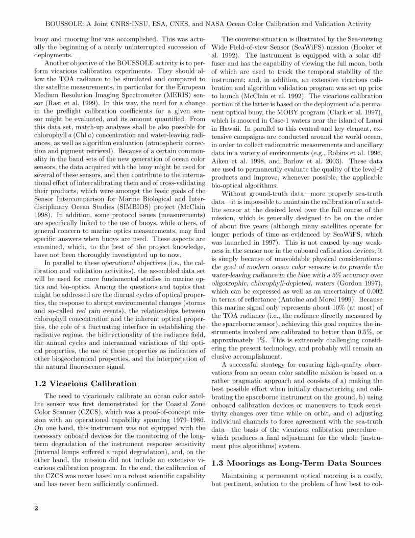
Accurate bathymetry data was a critical requirementfor properly deploying the taut mooring used to anchorthe buoy to the ocean floor (Sect. 5). The water depthat the proposed site was determined by performing sev-eral deep CTD casts, from which the measurement of thepressure (translated into depth using the simultaneous ob-servations of temperature and salinity), was added to themeasurement of an altimeter mounted on the CTD rosette(the CTD was stopped about 10 m before the bottom wasreached). The water-column thickness was, therefore, de-termined with a less than 1 m accuracy. These measure-ments were used to calibrate a two-dimensional mappingof the sea bottom that was obtained from the ship echosounder. This mapping revealed a flat bottom character-ized by a weak northwest-to-southeast slope (Fig. 2).
Fig. 2. The bathymetry, in meters, of the areaaround the BOUSSOLE site (at the crossing of thehorizontal and vertical lines). The open circles indi-cate the location of the individual deep CTD caststhat allowed the echo-sounder survey (grey dots) tobe calibrated in terms of water depth (gray-scalebar to the right of the plot).
The tidal amplitude, the dynamic height changes, andthe water level variations caused by atmospheric pressurechanges are all less than about 50 cm for the deployment
site, which is not significant for the type of mooring designenvisioned here. They might become problematic in thosecases wherein a similar mooring is deployed in another wa-ter mass where such changes are larger.
3.1.2 Physical Conditions
The BOUSSOLE site was selected in particular becausethe prevailing ocean currents are usually extremely weak.This peculiarity is due to the selected position being ratherclose to the center of the cyclonic circulation that char-acterizes the Ligurian Sea. The northern branch of thiscirculation is the Ligurian Current, which manifests as ajet flowing close to the shore in the northeast-to-southwestdirection which, in turn, establishes a front whose posi-tion varies seasonally (closer to shore in the winter than inthe summer). The southern branch of the circulation is asouthwest-to-northeast current flowing north of the islandof Corsica; the eastern part of the circulation is simplyimposed by the geometry of the basin.
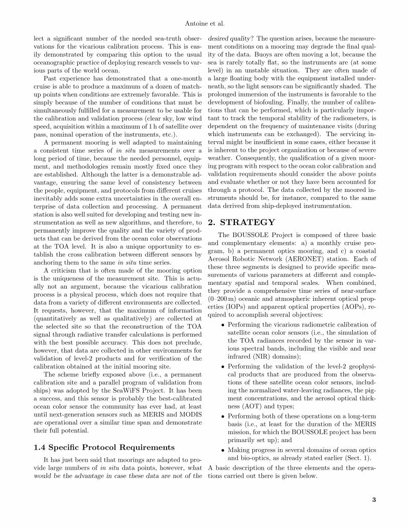
The dominant winds are from the west to southwestand from the northeast sectors (Fig. 3), and are channeledinto these two main directions by the general atmosphericcirculation of the region and by the topography formed bythe Alps and the island of Corsica. Over the period fromFebruary 1999 to July 2003, only five days were recordedwith a wind speed above 40 kts, and 34 and 100 days withwind speeds between 35–40 kts and 30–35 kts, respectively.These high wind speeds, and the associated large swells areconcentrated in the late fall to early spring time periods ofNovember to March, respectively.
Fig. 3. A so-called wind rose for the BOUSSOLEsite showing the dominant wind directions (the dataare from the Meteo buoy).
The range of environmental parameters is also illus-trated in Fig. 4, where physical conditions are displayedas a four-year record of the wind speed, significant waveheight, and sea surface temperature (SST). These data are
6

Antoine et al.
Fig. 4. An approximately five-year time series of conditions at the BOUSSOLE site showing a) the seasurface temperature, b) the swell height (the one-third most significant waves), and c) the wind speed.
7
BOUSSOLE: A Joint CNRS-INSU, ESA, CNES, and NASA Ocean Color Calibration and Validation Activity
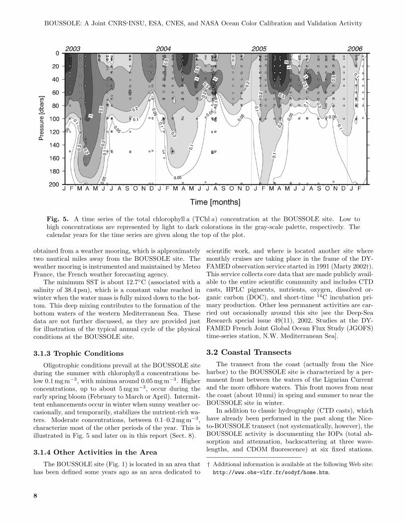
Fig. 5. A time series of the total chlorophyll a (TChl a) concentration at the BOUSSOLE site. Low tohigh concentrations are represented by light to dark colorations in the gray-scale palette, respectively. Thecalendar years for the time series are given along the top of the plot.
obtained from a weather mooring, which is aplproximatelytwo nautical miles away from the BOUSSOLE site. Theweather mooring is instrumented and maintained by MeteoFrance, the French weather forecasting agency.
The minimum SST is about 12.7◦C (associated with asalinity of 38.4 psu), which is a constant value reached inwinter when the water mass is fully mixed down to the bot-tom. This deep mixing contributes to the formation of thebottom waters of the western Mediterranean Sea. Thesedata are not further discussed, as they are provided justfor illustration of the typical annual cycle of the physicalconditions at the BOUSSOLE site.
3.1.3 Trophic Conditions
Oligotrophic conditions prevail at the BOUSSOLE siteduring the summer with chlorophyll a concentrations be-low 0.1 mg m−3, with minima around 0.05 mg m−3. Higherconcentrations, up to about 5 mg m−3, occur during theearly spring bloom (February to March or April). Intermit-tent enhancements occur in winter when sunny weather oc-casionally, and temporarily, stabilizes the nutrient-rich wa-ters. Moderate concentrations, between 0.1–0.2 mg m−3,characterize most of the other periods of the year. This isillustrated in Fig. 5 and later on in this report (Sect. 8).
3.1.4 Other Activities in the Area
The BOUSSOLE site (Fig. 1) is located in an area thathas been defined some years ago as an area dedicated to
scientific work, and where is located another site wheremonthly cruises are taking place in the frame of the DY-FAMED observation service started in 1991 (Marty 2002†).This service collects core data that are made publicly avail-able to the entire scientific community and includes CTDcasts, HPLC pigments, nutrients, oxygen, dissolved or-ganic carbon (DOC), and short-time 14C incubation pri-mary production. Other less permanent activities are car-ried out occasionally around this site [see the Deep-SeaResearch special issue 49(11), 2002, Studies at the DY-FAMED French Joint Global Ocean Flux Study (JGOFS)time-series station, N.W. Mediterranean Sea].
3.2 Coastal TransectsThe transect from the coast (actually from the Nice
harbor) to the BOUSSOLE site is characterized by a per-manent front between the waters of the Ligurian Currentand the more offshore waters. This front moves from nearthe coast (about 10 nmi) in spring and summer to near theBOUSSOLE site in winter.
In addition to classic hydrography (CTD casts), whichhave already been performed in the past along the Nice-to-BOUSSOLE transect (not systematically, however), theBOUSSOLE activity is documenting the IOPs (total ab-sorption and attenuation, backscattering at three wave-lengths, and CDOM fluorescence) at six fixed stations.
† Additional information is available at the following Web site:
http://www.obs-vlfr.fr/sodyf/home.htm.
8

Antoine et al.
Table 1. A summary of the types of data collected in support of the BOUSSOLE activity at the coastal, buoy, and shipsites (the latter is in very close proximity to the buoy). The above- and in-water references indicate how the oceanicdata are collected (for example, above- or in-water radiometers). The monthly service visits to the buoy, althoughsystematically scheduled, only occur if weather, site conditions (e.g., wave height), and instrument functionality permit.The data acquisition rates for the coastal and buoy continuous sampling are as follows, respectively: a) variable, downto 10 min; and b) 15 min (1 min at 6 Hz every 15 min from sunrise to sunset) plus 1 min at 6 Hz each hour duringnightime.
Sampling Data Instrument† Physical λ Data(and Site) Type or Model Measurements [nm] Products
Continuous Atmospheric CE-318 Sky radiances, and attenuation of λ6 Aerosol optical thick-(Coastal) the direct solar beam ness (τa) and types
Continuous Above-Water OCI-200 Downward irradiance λ7 Es
(Buoy) In-Water OCI-200 Downward irradiance at 4 and 9 m λ7 Ed
In-Water OCI-200 Upward irradiance at 4 and 9 m λ7 Eu
In-Water OCR-200 Upwelling radiance at 4 and 9 m λ7 Lu and LW
In-Water MINITracka Fluorescence at 4 and 9 m F ,[TChl a
]proxy
In-Water C-Star Beam attenuation at 9 m 660 cIn-Water SBE 37 SI Hydrography at 9 m T , S, and PIn-Water Hydroscat-II Backscattering at 9 m λ2 bb
In-Water EZ-III Tilt and heading at 9 m Tilt and heading‡Monthly Above-Water SIMBADA Total water radiance and atten- λ11 LW and τa
(Ship) uation of the direct solar beamAbove-Water OCI-1000 Downward irradiance λ13 Es
In-Water OCI-1000 Downward irradiance 0–150 m λ13 Ed
In-Water OCI-1000 Upward irradiance 0–150 m λ13 Eu and LW
In-Water SBE 911+ Hydrography 0–400 m T , S, P , F , and [O2]In-Water Rosette§ Discrete seawater samples 0–400 m Ci, ap, and aφ
In-Water AC-9+ Absorption, attenuation 0–400 m λ9 a, c, and b = c − aIn-Water ECO-BB3 Backscattering coefficient 0–400 m λ3 bb
In-Water C-STAR Attenuation coefficient 0–400 m λ1 cIn-Water WCF¶ CDOM fluorescence 0–400 m CDOM description
Notes:† Instrument names, as well as the corresponding manufacturers, are cited here, and in other sections of this report, because
they have been identified as appropriate for the particular application. This identification is not a recommendation for theuse of any of these instruments; nor does it imply that these instruments are the best suited for the application or for othersimilar projects. In addition, the possibility of using any other instrumentation than those cited here is retained withoutnotice.
‡ The buoy heading is used to determine the orientation of the in-water sensors, which are mounted on fixed arms, withrespect to the Sun.
§ SBE 12-bottle rosette for laboratory analyses of phytoplankton pigment concentrations (Ci) from HPLC; plus particles andphytoplankton absorption coefficients (ap and aφ, respectively).
¶ WETLabs CDOM Fluorometer.
λ1 660 nm.
λ2 442 and 560 nm.
λ3 470, 530, and 660 nm.
λ6 440, 675, 870 (plus 870 polarized), 940, and 1,020 nm.
λ7 412, 443, 490, 510, 560, 665, and 683 nm (a spare set of sensors have 443, 490, 510, 555, 560, 665, and 683 nm).
λ9 412, 443, 488, 510, 532, 555, 630, 676, and 715 nm.
λ11 350, 380, 412, 443, 490, 510, 565, 620, 670, 750, and 870 nm.
λ13 412, 443, 455, 490, 510, 530, 560, 620, 665, 683, 705, 780, and 865 nm before July 2003, and 380, 412, 443, 455, 490, 510,530, 560, 620, 665, 683, 705, and 780 nm thereafter.
9
BOUSSOLE: A Joint CNRS-INSU, ESA, CNES, and NASA Ocean Color Calibration and Validation Activity
The stations are approximately 5 nmi away from one an-other, and the survey work started in May of 2003. Docu-menting these properties at this series of stations is also away to put the observations made at the BOUSSOLE siteinto a broader context.
3.3 The Coastal AERONET SiteAerosol amounts and types are information of prime
importance in the process of vicariously calibrating oceancolor sensors (Sect. 10), but they cannot be obtained easilyat the mooring site. This is the main reason for havinginstalled an automatic scanning sun and sky photometer atCap Ferrat, which is providing a continuous record (cloudpermitting) of these parameters thanks to the logistics anddata transmission capabilities of the AERONET.
The parallel analysis of the sun photometer and satel-lite observations are expected to indicate the circumstanceswherein the data collected at the coast are representative ofthe conditions offshore. In support of this study, aerosol—and when the sky is clear—optical thickness measurementsare also performed en route when steaming from Nice tothe BOUSSOLE site, in order to get some idea of the spa-tial heterogeneity of aerosol properties.
4. DATA COLLECTIONThe three subsections below briefly summarize the set
of measurements that are performed offshore, either fromthe ship or from the buoy, and at the coastal site. Theyare summarized in Table 1. Details on the data acquisitionprotocols will be provided in Sect. 6 and data processingin Sect. 7.
4.1 Ship MeasurementsThe set of parameters directly derived from the mea-
surements made by the above-water SeaWiFS Multichan-nel Surface Reference (SMSR) and the in-water SPMR to200 m depth are as follows (λ13 denotes the 13-channelspectral band set): a) surface irradiance, Es(λ13), and b)upward and downward irradiance, Eu(λ13) and Ed(λ13),respectively. The wavelengths for these measurements are380, 411, 443, 456, 491, 510, 532, 560, 620, 665, 683, 705,779, and 865 nm
Profiles with the CTD rosette to a depth of 400 m areused to collect the following parameters: chlorophyll fluo-rescence, CDOM fluorescence, attenuation and absorptioncoefficients (412, 440, 488, 510, 532, 555, 630, 676, and715 nm), bb (440, 532, and 650), temperature, conductiv-ity and derived salinity, oxygen concentration, and surfacePAR. Seawater samples are collected and filtered for sub-sequent determination of the phytoplankton pigments andparticulate absorption.
The SIMBADA above-water radiometer collects water-leaving radiance and aerosol optical thickness at 350, 380,412, 443, 490, 510, 565, 620, 670, 750, and 870 nm.
4.2 Buoy Measurements
The set of parameters directly derived from the buoyabove- and in-water measurements are as follows (λ7 de-notes the 7-channel spectral band set for the AOP sensors):a) Es(λ7); b) Ed(λ7), Eu(λ7), Lu(λ7), c(660), and chloro-phyll fluorescence at 4 m; and c) Ed(λ7), Eu(λ7), Lu(λ7),chlorophyll fluorescence, c(660), bb(443), and bb(560), con-ductivity, temperature, pressure, and two-axis tilt as wellas compass heading at 9 m. The wavelengths for the AOPmeasurements are 412, 443, 490, 510, 560, 665, and 683 nm(a spare set of sensors has the 412 nm channel replaced with555 nm).
From these measurements, various AOPs or IOPs arederived: the diffuse attenuation coefficients for upward anddownward irradiance, Ku and Kd; the attenuation coeffi-cient for upwelling radiance, KL; the diffuse reflectancejust below the sea surface, R; the nadir Q-factor, Eu/Lu;and the attenuation and backscattering coefficients, c andbb. The absorption coefficient, a, is tentatively derivedthrough inversion of the AOPs (using, for example, Kd
and R). Here it is assumed that Kd and R can be ac-curately derived from the two measurement depths of thebuoy, e.g., Gordon and Boynton (1997), Leathers and Mc-Cormick (1997), and Barnard et al. (1999). Table 2 showshow the data acquired on the system fits to the band setsof several ocean color sensors.
Table 2. The MERIS wavelengths, as acquired onthe buoy (leftmost column), and the spectral shiftof other satellite bands with respect to those ofMERIS. The second row gives the channel band-widths.
MERIS POLDER-3 SeaWiFS MODIS10 nm 20 nm 20 nm 10 nm
412 nm 0 0443 0 0 0490 0 0 −2510 0560 +5 −5 −9665 +5 +5 +2683 0
The data are derived from the IOCCG (1998) report.
4.3 Coastal Measurements
The parameters collected at the coastal site are the sunand sky radiances, using standard filters at 440, 675, 870,940, and 1,020 nm plus a polarized filter for 870 nm, whichare used to derive total column water vapor, ozone, andaerosol properties, including Angstrom coefficients, opticalthickness, and polarization ratios†.
† These derived parameters are available at two WorldwideWeb addresses: http://www-loa.univ-lille1.fr/photons/DATA/Villefranche and http://aeronet.gsfc.nasa.gov.
10
Upp
er S
uper
stru
ctur
eLo
wer
Sup
erst
ruct
ure
SensorArm
SolarPanel
BuoyancySphere
Antoine et al.
5. THE BOUSSOLE BUOYThe description of the BOUSSOLE buoy is presented
more or less in a chronological order, starting with thedesign, and then continuing with the successive versionsand the various tests that were performed.
5.1 Design ConceptPlatforms developed for oceanographic purposes are
rarely adapted to the unique problems of deploying ra-diometers. Accurately measuring the in-water light fieldis difficult, because the instruments themselves and, usu-ally more significantly, the platform onto which they areinstalled, introduce perturbations (shading in particular).Other difficulties originate from the need to keep the in-struments oriented as stably as possible, either because anadir radiance or a planar irradiance is being measured.The actual measurement depth can also be difficult to ac-curately assess, because rapid vertical displacements of theinstruments sometimes occur, which prevent any preciseestimation of pressure (and, thus, depth). Considering theabove difficulties (among others), a new type of platformwas developed and specifically dedicated to making high-quality radiometric measurements at sea. The platformminimizes shading effects by reducing the cross-sectionalarea of structural components, and its wave-interactioncharacteristics ensure the stability of the instruments.
The design constraints for the new platform were:1. Measure Eu, Ed, and Lu (nadir) at two depths, plus
Es at the surface;2. Minimize the shading of the instruments;3. Maximize the stability of the instruments; and4. Permit deployment at a site with a water depth of
2,440 m, and swells up to 8 m (but small horizontalcurrents).
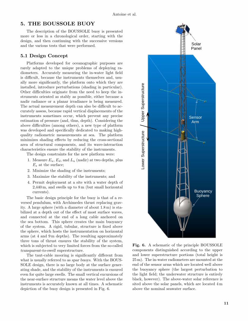
The basic design principle for the buoy is that of a re-versed pendulum, with Archimedes thrust replacing grav-ity. A large sphere (with a diameter of about 1.8 m) is sta-bilized at a depth out of the effect of most surface waves,and connected at the end of a long cable anchored onthe sea bottom. This sphere creates the main buoyancyof the system. A rigid, tubular, structure is fixed abovethe sphere, which hosts the instrumentation on horizontalarms (at 4 and 9 m depths). The resulting approximatelythree tons of thrust ensures the stability of the system,which is subjected to very limited forces from the so-calledtransparent-to-swell superstructure.
The taut-cable mooring is significantly different fromwhat is usually referred to as spar buoys. With the BOUS-SOLE design, there is no large body at the surface gener-ating shade, and the stability of the instruments is ensuredeven for quite large swells. The small vertical excursions ofthe near-surface structure means the water level above theinstruments is accurately known at all times. A schematicdepiction of the buoy design is presented in Fig. 6.
Fig. 6. A schematic of the principle BOUSSOLEcomponents distinguished according to the upperand lower superstructure portions (total height is25 m). The in-water radiometers are mounted at theend of the sensor arms which are located well abovethe buoyancy sphere (the largest perturbation tothe light field; the underwater structure is entirelyblack, however). The above-water solar reference issited above the solar panels, which are located 4 mabove the nominal seawater surface.
11
BOUSSOLE: A Joint CNRS-INSU, ESA, CNES, and NASA Ocean Color Calibration and Validation Activity
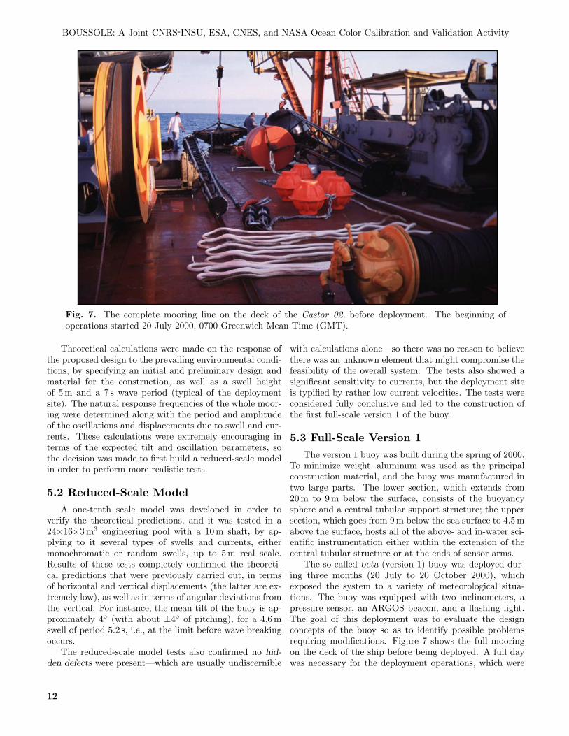
Fig. 7. The complete mooring line on the deck of the Castor–02, before deployment. The beginning ofoperations started 20 July 2000, 0700 Greenwich Mean Time (GMT).
Theoretical calculations were made on the response ofthe proposed design to the prevailing environmental condi-tions, by specifying an initial and preliminary design andmaterial for the construction, as well as a swell heightof 5 m and a 7 s wave period (typical of the deploymentsite). The natural response frequencies of the whole moor-ing were determined along with the period and amplitudeof the oscillations and displacements due to swell and cur-rents. These calculations were extremely encouraging interms of the expected tilt and oscillation parameters, sothe decision was made to first build a reduced-scale modelin order to perform more realistic tests.
5.2 Reduced-Scale ModelA one-tenth scale model was developed in order to
verify the theoretical predictions, and it was tested in a24×16×3 m3 engineering pool with a 10 m shaft, by ap-plying to it several types of swells and currents, eithermonochromatic or random swells, up to 5 m real scale.Results of these tests completely confirmed the theoreti-cal predictions that were previously carried out, in termsof horizontal and vertical displacements (the latter are ex-tremely low), as well as in terms of angular deviations fromthe vertical. For instance, the mean tilt of the buoy is ap-proximately 4◦ (with about ±4◦ of pitching), for a 4.6 mswell of period 5.2 s, i.e., at the limit before wave breakingoccurs.
The reduced-scale model tests also confirmed no hid-den defects were present—which are usually undiscernible
with calculations alone—so there was no reason to believethere was an unknown element that might compromise thefeasibility of the overall system. The tests also showed asignificant sensitivity to currents, but the deployment siteis typified by rather low current velocities. The tests wereconsidered fully conclusive and led to the construction ofthe first full-scale version 1 of the buoy.
5.3 Full-Scale Version 1The version 1 buoy was built during the spring of 2000.
To minimize weight, aluminum was used as the principalconstruction material, and the buoy was manufactured intwo large parts. The lower section, which extends from20 m to 9 m below the surface, consists of the buoyancysphere and a central tubular support structure; the uppersection, which goes from 9 m below the sea surface to 4.5 mabove the surface, hosts all of the above- and in-water sci-entific instrumentation either within the extension of thecentral tubular structure or at the ends of sensor arms.
The so-called beta (version 1) buoy was deployed dur-ing three months (20 July to 20 October 2000), whichexposed the system to a variety of meteorological situa-tions. The buoy was equipped with two inclinometers, apressure sensor, an ARGOS beacon, and a flashing light.The goal of this deployment was to evaluate the designconcepts of the buoy so as to identify possible problemsrequiring modifications. Figure 7 shows the full mooringon the deck of the ship before being deployed. A full daywas necessary for the deployment operations, which were
12
Per
cent
age
of D
ays
[%]
E
E
EE
EE
E E
E
0
30
60
90
0 30 60 90Days
Antoine et al.
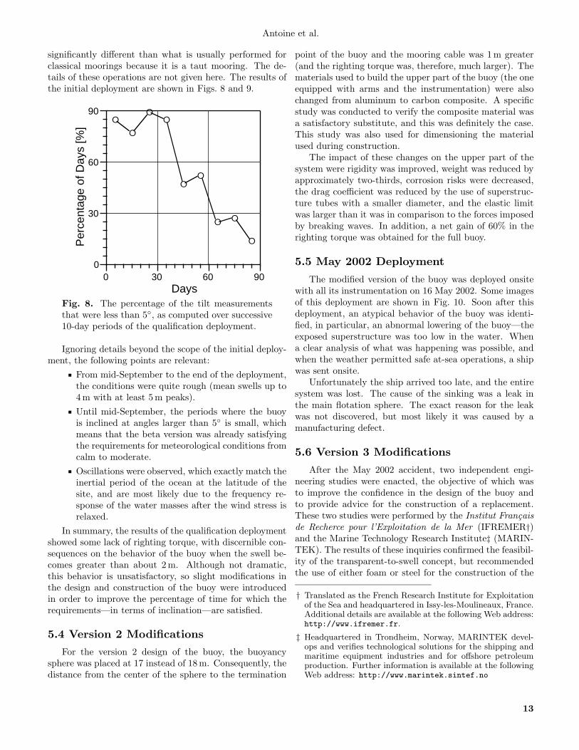
significantly different than what is usually performed forclassical moorings because it is a taut mooring. The de-tails of these operations are not given here. The results ofthe initial deployment are shown in Figs. 8 and 9.
Fig. 8. The percentage of the tilt measurementsthat were less than 5◦, as computed over successive10-day periods of the qualification deployment.
Ignoring details beyond the scope of the initial deploy-ment, the following points are relevant:
From mid-September to the end of the deployment,the conditions were quite rough (mean swells up to4 m with at least 5 m peaks).Until mid-September, the periods where the buoyis inclined at angles larger than 5◦ is small, whichmeans that the beta version was already satisfyingthe requirements for meteorological conditions fromcalm to moderate.Oscillations were observed, which exactly match theinertial period of the ocean at the latitude of thesite, and are most likely due to the frequency re-sponse of the water masses after the wind stress isrelaxed.
In summary, the results of the qualification deploymentshowed some lack of righting torque, with discernible con-sequences on the behavior of the buoy when the swell be-comes greater than about 2 m. Although not dramatic,this behavior is unsatisfactory, so slight modifications inthe design and construction of the buoy were introducedin order to improve the percentage of time for which therequirements—in terms of inclination—are satisfied.
5.4 Version 2 Modifications
For the version 2 design of the buoy, the buoyancysphere was placed at 17 instead of 18 m. Consequently, thedistance from the center of the sphere to the termination
point of the buoy and the mooring cable was 1 m greater(and the righting torque was, therefore, much larger). Thematerials used to build the upper part of the buoy (the oneequipped with arms and the instrumentation) were alsochanged from aluminum to carbon composite. A specificstudy was conducted to verify the composite material wasa satisfactory substitute, and this was definitely the case.This study was also used for dimensioning the materialused during construction.
The impact of these changes on the upper part of thesystem were rigidity was improved, weight was reduced byapproximately two-thirds, corrosion risks were decreased,the drag coefficient was reduced by the use of superstruc-ture tubes with a smaller diameter, and the elastic limitwas larger than it was in comparison to the forces imposedby breaking waves. In addition, a net gain of 60% in therighting torque was obtained for the full buoy.
5.5 May 2002 Deployment
The modified version of the buoy was deployed onsitewith all its instrumentation on 16 May 2002. Some imagesof this deployment are shown in Fig. 10. Soon after thisdeployment, an atypical behavior of the buoy was identi-fied, in particular, an abnormal lowering of the buoy—theexposed superstructure was too low in the water. Whena clear analysis of what was happening was possible, andwhen the weather permitted safe at-sea operations, a shipwas sent onsite.
Unfortunately the ship arrived too late, and the entiresystem was lost. The cause of the sinking was a leak inthe main flotation sphere. The exact reason for the leakwas not discovered, but most likely it was caused by amanufacturing defect.
5.6 Version 3 Modifications
After the May 2002 accident, two independent engi-neering studies were enacted, the objective of which wasto improve the confidence in the design of the buoy andto provide advice for the construction of a replacement.These two studies were performed by the Institut Francaisde Recherce pour l’Exploitation de la Mer (IFREMER†)and the Marine Technology Research Institute‡ (MARIN-TEK). The results of these inquiries confirmed the feasibil-ity of the transparent-to-swell concept, but recommendedthe use of either foam or steel for the construction of the
† Translated as the French Research Institute for Exploitationof the Sea and headquartered in Issy-les-Moulineaux, France.Additional details are available at the following Web address:http://www.ifremer.fr.
‡ Headquartered in Trondheim, Norway, MARINTEK devel-ops and verifies technological solutions for the shipping andmaritime equipment industries and for offshore petroleumproduction. Further information is available at the followingWeb address: http://www.marintek.sintef.no
13
BOUSSOLE: A Joint CNRS-INSU, ESA, CNES, and NASA Ocean Color Calibration and Validation Activity
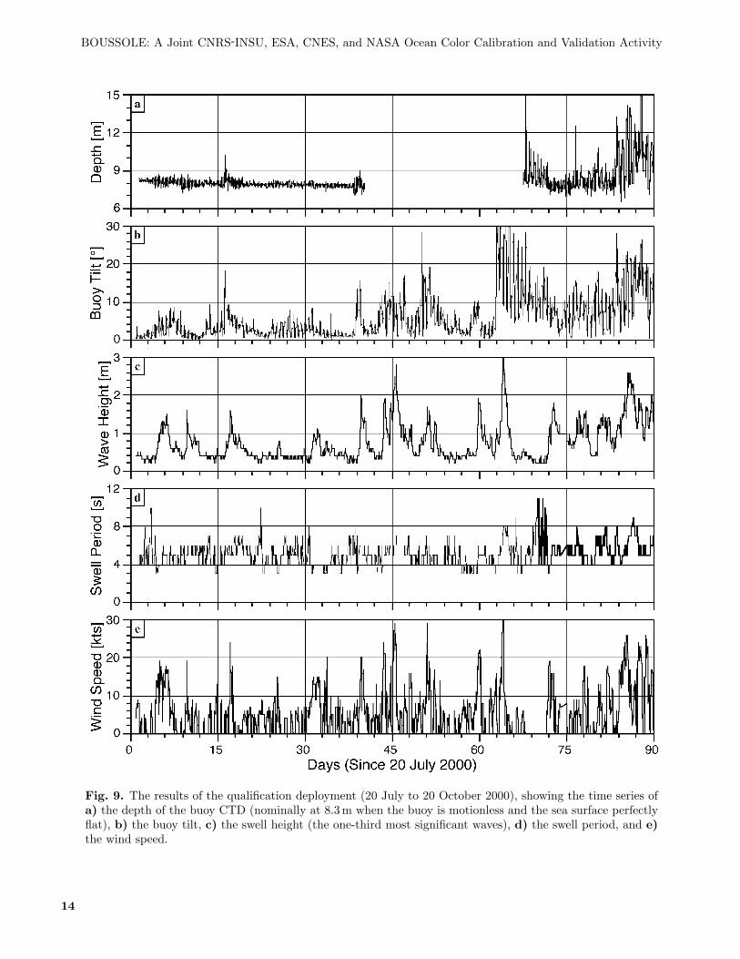
Fig. 9. The results of the qualification deployment (20 July to 20 October 2000), showing the time series ofa) the depth of the buoy CTD (nominally at 8.3 m when the buoy is motionless and the sea surface perfectlyflat), b) the buoy tilt, c) the swell height (the one-third most significant waves), d) the swell period, and e)the wind speed.
14
Antoine et al.
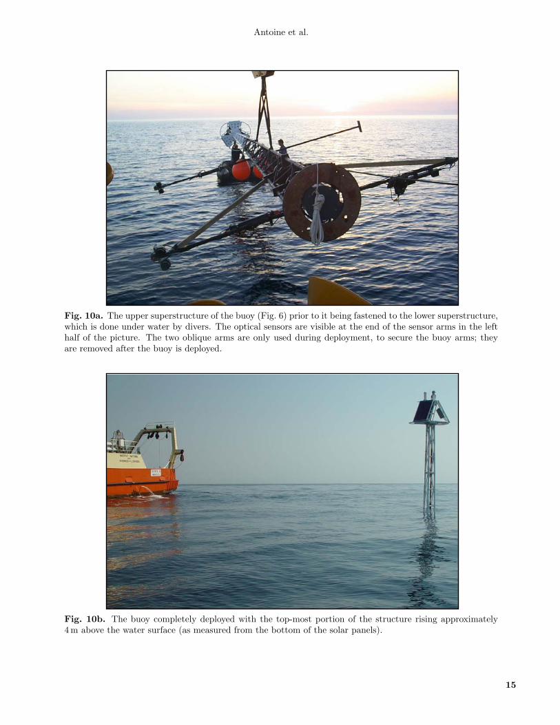
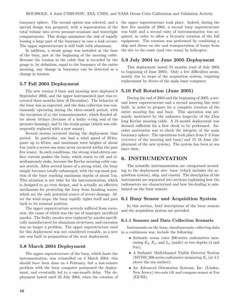
Fig. 10a. The upper superstructure of the buoy (Fig. 6) prior to it being fastened to the lower superstructure,which is done under water by divers. The optical sensors are visible at the end of the sensor arms in the lefthalf of the picture. The two oblique arms are only used during deployment, to secure the buoy arms; theyare removed after the buoy is deployed.
Fig. 10b. The buoy completely deployed with the top-most portion of the structure rising approximately4 m above the water surface (as measured from the bottom of the solar panels).
15
BOUSSOLE: A Joint CNRS-INSU, ESA, CNES, and NASA Ocean Color Calibration and Validation Activity
buoyancy sphere. The second option was selected, and aspecial design was prepared, with a segmentation of thetotal volume into seven pressure-resistant and watertightcompartments. This design minimizes the risk of rapidlyloosing a large part of the buoyancy in case a leak occurs.The upper superstructure is still built with aluminum.
In addition, a strain gauge was installed at the baseof the buoy, just at the beginning of the mooring cable.Because the tension in the cable that is recorded by thegauge is, by definition, equal to the buoyancy of the entiremooring, any change in buoyancy can be detected as achange in tension.
5.7 Fall 2003 Deployment
The new version 3 buoy and mooring were deployed 6September 2003, and the upper instrumented part was re-covered three months later (6 December). The behavior ofthe buoy was as expected, and the data collection was con-tinuously operating during the three-month period, withthe exception of a) the transmissometer, which flooded af-ter about 10 days (because of a faulty o-ring seal of thepressure housing); and b) the strain gauge (which was sub-sequently replaced with a new sensor).
Several storms occurred during the deployment timeperiod. In particular, one had a wind speed of 50 kts,gusts up to 65 kts, and maximum wave heights of about8 m (such a severe sea state never occurred within the pastfive years). In such conditions, the strong wind-driven sur-face current pushes the buoy, which starts to tilt and si-multaneously sinks, because the Kevlar mooring cable can-not stretch. After several hours of a strong wind, the buoysimply becomes totally submerged, with the top-most por-tion of the buoy reaching maximum depths of about 5 m.This situation is not risky for the instrumentation, whichis designed to go even deeper, and is actually an effectivemechanism for protecting the buoy from breaking waves,which are the only potential source of severe damage. Af-ter the wind stops, the buoy rapidly rights itself and goesback to its nominal position.
The upper superstructure severely suffered from corro-sion, the cause of which was the use of improper sacrificialanodes. The faulty anodes were replaced by anodes specifi-cally manufactured for aluminum structures, and corrosionwas no longer a problem. The upper superstructure usedfor this deployment was not considered reusable, so a newone was built in preparation of the next deployment.
5.8 March 2004 Deployment
The upper superstructure of the buoy, which hosts theinstrumentation, was reinstalled on 4 March 2004; thisshould have been done on 4 February, but a last-minuteproblem with the buoy computer postponed the deploy-ment, and eventually led to a one-month delay. The de-ployment lasted until 23 July 2004, when the rotation of
the upper superstructure took place. Indeed, during thefirst five months of 2004, a second buoy superstructurewas built and a second suite of instrumentation was ac-quired, in order to allow a bi-yearly rotation of the fullequipment. The rotation was performed by combining aship and divers on site and transportation of buoys fromthe site to the coast (and vice versa) by helicopter.
5.9 July 2004 to June 2005 DeploymentThis deployment lasted 10 months (end of July 2004
to beginning of June 2005). Only a few difficulties arose,mostly due to stops of the acquisition system, requiringreplacement by divers of the main buoy computer.
5.10 Full Rotation (June 2005)During the end of 2004 and the beginning of 2005, a sec-
ond lower superstructure and a second mooring line werebuilt, in order to prepare for a complete rotation of theentire mooring line and buoy. This operation was pri-marily motivated by the unknown longevity of the 2 kmlong Kevlar mooring cable. A 21-month deployment wasdeemed sufficient for a first check to be performed. An-other motivation was to check the integrity of the mainbuoyancy sphere. The operations took place from 2–3 June(recovery of the mooring and buoy) and 15–16 June (de-ployment of the new system). The system has been at seasince then.
6. INSTRUMENTATIONThe scientific instrumentation are categorized accord-
ing to the deployment site: buoy (which includes the ac-quisition system), ship, and coastal. The description of theinstruments are separated into sections explaining how theradiometers are characterized and how bio-fouling is min-imized on the buoy sensors.
6.1 Buoy Sensor and Acquisition SystemIn this section, brief descriptions of the buoy sensors
and the acquisition system are provided.
6.1.1 Sensors and Data Collection Scenario
Instruments on the buoy, simultaneously collecting datain a continuous way, include the following:
• Satlantic ocean color 200-series radiometers mea-suring Ed, Eu, and Lu (nadir) at two depths (4 and9 m);
• A Satlantic Multichannel Visible Detector System(MVDS) 200-series radiometer measuring Es (at 4.5above the sea surface);
• An Advanced Orientation Systems, Inc. (Linden,New Jersey) two-axis tilt and compass sensor at 9 m(EZ-III);
16
Antoine et al.
• A Sea-Bird Electronics, Inc. (Bellevue, Washing-ton) CTD at 9 m measuring conductivity, tempera-ture, and pressure.
• Chelsea (Surrey, United Kingdom) MINItracka MkII fluorometers at 4 and 9 m for a proxy for theTChl a concentration,
[TChl a
].
• WETLabs C-star transmissometers at 4 and 9 m forthe beam attenuation coefficient at 660 nm, a proxyof the particle load.
• A Hydro-Optics, Biology, and InstrumentationLaboratories (HOBI Labs), Inc. (Tucson, Arizona)Hydroscat-II backscattering meter at 9 m measur-ing a proxy to bb(λ) at two wavelengths (442 and560 nm).
These data are collected every 15 min during daylight, andat hourly intervals at night. Each data acquisition se-quence lasts one minute.
6.1.2 The Integrated Acquisition System
The central recording device of the buoy is the DataAquisition and Control Network (DACNet) unit, whichhouses the primary computer: a PC104 Cool RoadRunnerII 200 MHz 6×86 with 32 MB of random access memory(RAM) and the serial data acquisition equipment (record-ing to a 1 GB disk drive). These components are used inthe collection, storage, and downloading of the data ob-tained from the instruments. The majority of the time thesystem is inactive, and the DACNet unit is unpowered. Asmall internal microcontroller is responsible for the powersupervision and control, and a precision clock.
Optimization of the power budget is an important el-ement, because of the restricted power available from the12 VDC 105 Ah underwater battery, which is recharged us-ing solar panels. The power managment functions can besummarized as follows:
1. An accurate real-time clock;2. An alarm clock for powering up the system for the
programmed schedule;3. A watchdog timer that protects against draining the
battery in the event of a computer malfunction; and4. A power-fail shutdown to prevent computer startup
if the battery power is too low.The DACNet operating system runs on Red Hat Linux6.2 kernel v2.2.19, which accommodates custom-made Javasoftware: the Satlantic Telemetry Acquisition Manager(STAM) and the Satlantic Node Manager. These pro-grams provide the operational, configuration, and interfacerequirements for the buoy to run autonomously and enablecommunication of data and files with the user.
A third piece of software, Satlantic Base Manager, runson a personal computer (PC) equipped with the WindowsNT or Windows 98 operating system and provides the op-erator with administrative tools—each with a graphical
user interface (GUI). These tools enable the user to con-figure the Node Manager, transfer data and files, updatethe internal clock of the acquisition node, view data fromspecified instruments in real time, and completely shut-down the acquisition node for maintenance†.
6.1.3 Data Communications
The complete data stream can be downloaded througha wireless ethernet link established between the buoy andthe ship (the same equipment is used aboard the buoy andthe ship). This link functions with the ship positioneda few hundred meters from the buoy. The connection isdriven by the buoy, with a wakeup sequence each hourof the day. This hierarchy was adopted, rather than es-tablishing the communication from the ship, in order tominimize the time during which the buoy communicationhardware is awake and consuming energy.
Data retrieval from the buoy is performed from theDACNet via a Cisco Aironet 340 series wireless bridgemanufactured by Cisco Systems (San Jose, California) andis stored directly on a PC. The data is retrieved in a bi-nary format and consists of one daily log file for eachof the following seven groups: a) the instruments con-nected to the DATA-100 at 4 m (radiometers and fluorom-eter); b) the instruments connected to the data acquisi-tion module (DATA-100) at 9 m (radiometers, fluorometer,transmissometer); c) the CTD; d) the Hydroscat-II; e) thestrain gauge; f) the MVDS; and g) the two-axis tilt sensorand compass. The daily file is closed once communicationthrough the Cisco system occurs. In this case, a new file iscreated starting from the next measurement taken by theDACNet system until midnight or until a subsequent linkup via the Cisco system is performed. Storage space onthe hard disk of the DACNet has the capacity to store upto approximately three months of data.
Part of the data stream is transmitted via the ARGOSsystem and is used for surveying the functioning of thesystem; the sample data include the tilt and depth of thebuoy, the strain of the mooring cable, the battery voltage,the disk space, the spectrum of the above-water irradiance,and instrument health parameters, which are indicatingwhether or not instruments and the acquisition system arefunctioning nominally.
6.2 Shipboard SensorsIn this section, brief descriptions are provided of the
instruments deployed from the ship to help characterize theBOUSSOLE site during the monthly maintenance cruises.The objective here is to have quality-assured data for themost important hydrographic, optical (AOPs and IOPs),and biogeochemical parameters.
† More details of this software can be found in Satlantic’s man-ual DACNet Software Overview—Villefranche Remote Opti-cal Mooring.
17
JJ J J J JJ J J J J
EE E E E EE E E E E
-0.005
0
0.005
0.010
0.015
-5 5 15 25 35
Res
idua
l [°C
]
Temperature [°C]
J Calibration 10Jan03
E Calibration 28Jan02
J JJ JJ JEEE
EE E
-0.002
-0.001
0
0.001
0.002
0 2 4 6
Res
idua
l [S
/m]
Conductivity [S/m]
J Calibration 29Jan02
E Calibration 03Jan01
BOUSSOLE: A Joint CNRS-INSU, ESA, CNES, and NASA Ocean Color Calibration and Validation Activity
6.2.1 CTD and Water Sampling
The CTD/rosette package is based on a Sea-Bird Elec-tronics (SBE) 911 plus, equipped with the following sen-sors:
Pressure (Digiquartz Paroscientific, Inc.);Temperature (SBE 3);Conductivity (SBE 4);Dissolved oxygen (SBE 13 until January 2003, andthen an SBE 43); andAltimeter (Datasonics PSA 900).
The sensors are mounted on a SBE 32 rosette with 11 12 LNiskin bottles (the 12th being replaced by an AC-9+ asdiscussed below).
The pressure sensor is not regularly calibrated (it waslast calibrated in 1995); it is known from past experiencewith this type of sensor that the uncertainty is on the orderof 0.5 dbar. It is acknowledged that this type of sensoronly experiences a drift of the zero point, which is easyto control, and to correct for, when the sensor is at thesurface.
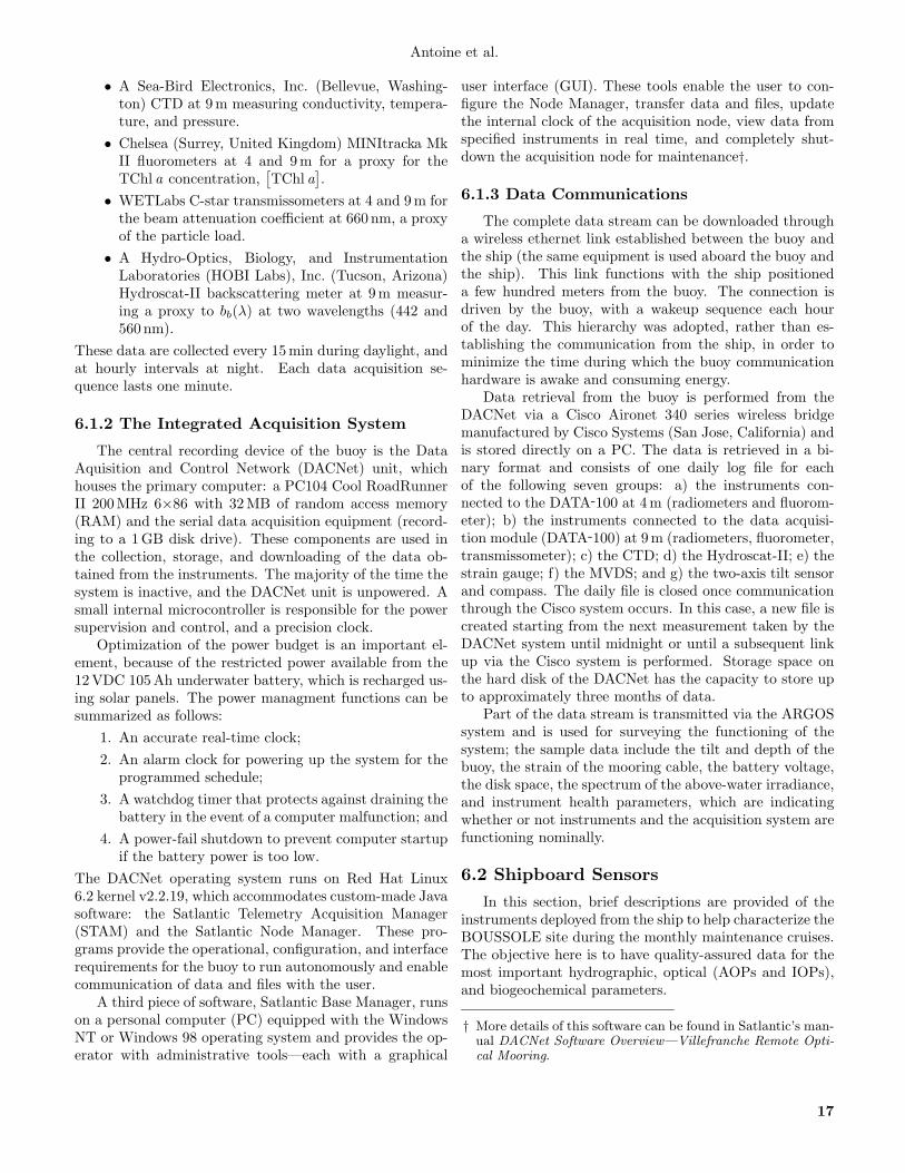
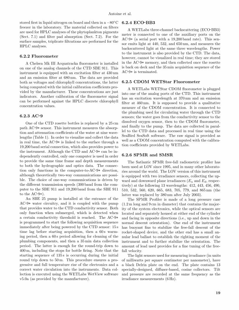
The temperature sensor is sent once a year for calibra-tion to SBE, which has the agreement from the NationalInstitute of Standards and Technology (NIST) for this typeof work. Figure 11 provides an example of the calibrationsperformed in January 2002 and January 2003 (was aboutthe same between January of 2001 and January of 2002).The drift is on the order of 0.0025◦C over one year, and itis linear. Any temperature value computed between two ofthese calibrations is, therefore, provided with a ±0.0025◦Cuncertainty.
Fig. 11. The calibration drift of the temperaturesensor mounted on the CTD.
The conductivity sensor is sent once a year to SBE forcalibration. Additional calibration against values deter-mined from water samples and subsequent laboratory anal-yses (with a laboratory salinometer) are not performed.
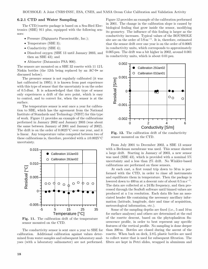
Figure 12 provides an example of the calibration performedin 2001. The change in the calibration slope is caused bybiological fouling that grow inside the sensor, modifyingits geometry. The influence of this fouling is larger as theconductivity increases. Typical values of the BOUSSOLEsite are on the order of 5 S m−1. It is, therefore, estimatedthat the sensor drift over one year is on the order of 0.0005in conductivity units, which corresponds to approximately0.005 psu. The drift was a bit higher in 2002, around 0.001in conductivity units, which is about 0.01 psu.
Fig. 12. The calibration drift of the conductivitysensor mounted on the CTD.
From July 2001 to December 2002, a SBE 13 sensorwith a Beckman membrane was used. This sensor showeda large drift. Starting in January of 2003, a new sensorwas used (SBE 43), which is provided with a nominal 5%uncertainty and a less than 2% drift. No Winkler-basedcalibrations are performed on these sensors.
At each cast, a first round trip down to 50 m is per-formed with the CTD, in order to rinse all instrumentsand equilibrate them in temperature. Then the package islowered down to 400 m at a descent rate of about 0.5 m s−1.The data are collected at a 24 Hz frequency, and then pro-cessed through the SeaSoft software until binned values areproduced at a 1 m resolution. Each data file has an asso-ciated header file containing the necessary ancillary infor-mation (latitude, longitude, date and time of acquisition,meteorological information, etc.).
Some of the sampling depths are fixed (i.e., 5 and 10 mfor surface analyses) and others are determined at the endof the rosette descent, based on the phytoplankton flu-orescence profile, in order to best represent any specificfeatures of the vertical profile. No sampling is done deeperthan 200 m. Bottles are closed during the ascent of therosette. When back on deck, 2.8 L plastic bottles are usedto collect water that is used for subsequent filtration. Thefilters are kept in Petri slides, wrapped in aluminum and
18
Antoine et al.
stored first in liquid nitrogen on board and then in a −80◦Cfreezer in the laboratory. The material collected on filtersare used for HPLC analyses of the phytoplankton pigments(Sect. 7.1) and filter pad absorption (Sect. 7.2). For thesurface samples, triplicate filtrations are performed for theHPLC analyses.
6.2.2 Fluorometer
A Chelsea Mk III Acquatracka fluorometer is installedon one of the analog channels of the CTD SBE 911. Thisinstrument is equipped with an excitation filter at 430 nmand an emission filter at 680 nm. The data are providedboth as voltages and chlorophyll concentrations, the latterbeing computed with the initial calibration coefficients pro-vided by the manufacturer. These concentrations are justindicators. Another calibration of the fluorometer signalcan be performed against the HPLC discrete chlorophyllconcentration values.
6.2.3 AC-9
One of the CTD rosette bottles is replaced by a 25 cmpath AC-9+ sensor. This instrument measures the absorp-tion and attenuation coefficients of the water at nine wave-lengths (Table 1). In order to visualize and collect the datain real time, the AC-9+ is linked to the surface through a19,200 baud serial connection, which also provides power tothe instrument. Although the CTD and AC-9+ can be in-dependently controlled, only one computer is used in orderto provide the same time frame and depth measurementsto both the hydrographic and optics data. The connec-tion only functions in the computer-to-AC-9+ direction,although theoretically two-way communications are possi-ble. The choice of one-way communications is driven bythe different transmission speeds (300 baud from the com-puter to the SBE 911 and 19,200 baud from the SBE 911to the AC-9+).
An SBE 25 pump is installed at the entrance of theAC-9+ water circuitry, and it is coupled with the pumpthat provides water to the CTD conductivity sensor. Bothonly function when submerged, which is detected whena certain conductivity threshold is reached. The AC-9+is programmed to start the following acquisition sequenceimmediately after being powered by the CTD sensor: 15 stime lag before starting acquisition, then a 60 s warm-ing period, then a 60 s period allowing for cleaning of theplumbing components, and then a 35 min data collectionperiod. The latter is enough for the round-trip down to400 m, including the stops for bottle firing. Note that thestarting sequence of 135 s is occurring during the initialround trip down to 50 m. This procedure ensures a pro-gressive and full temperature rise of the electronics and acorrect water circulation into the instruments. Data col-lection is executed using the WETLabs WetView softwarev5.0a (as provided by the manufacturer).
6.2.4 ECO-BB3
A WETLabs three-channel backscattering (ECO-BB3)meter is connected to one of the auxiliary ports on theAC-9+ (a serial port with a 19,200 baud rate). This sen-sor emits light at 440, 532, and 650 nm, and measures thebackscattered light at the same three wavelengths. Powerto the instrument is also provided by the CTD. The data,however, cannot be visualized in real time; they are storedin the AC-9+ memory, and then collected once the rosetteis back on deck and the 35 min acquisition sequence of theAC-9+ is terminated.
6.2.5 CDOM WETStar Fluorometer
A WETLabs WETStar CDOM fluorometer is pluggedinto one of the analog ports of the CTD. This instrumenthas an excitation wavelength at 370 nm and an emissionfilter at 460 nm. It is supposed to provide a qualitativemeasure of the CDOM concentration. It is connected tothe plumbing used for circulating water through the CTDsensors; the water goes from the conductivity sensor to thedissolved oxygen sensor, then to the CDOM fluorometer,and finally to the pump. The data are collected in paral-lel to the CTD data and processed in real time using theSeaBird SeaSoft software. The raw signal is provided aswell as a CDOM concentration computed with the calibra-tion coefficients provided by WETLabs.
6.2.6 SPMR and SMSR
The Satlantic SPMR free-fall radiometric profiler hasbeen used at LOV since 1995, and in many other laborato-ries around the world. The LOV version of this instrumentis equipped with two irradiance sensors, collecting the up-ward and downward plane irradiances (Eu and Ed, respec-tively) at the following 13 wavelengths: 412, 443, 456, 490,510, 532, 560, 620, 665, 683, 705, 779, and 865 nm (thelatter was replaced by 380 nm after July 2003).
The SPMR Profiler is made of a long pressure case(1.2 m long and 9 cm in diameter) that contains the major-ity of the system electronics, while the optical sensors arelocated and separately housed at either end of the cylinderand facing in opposite directions (i.e., up and down in thenormal descent orientation). One end of the instrumenthas buoyant fins to stabilize the free-fall descent of therocket-shaped device, and the other end has a small an-nular lead ballast to establish the righting moment of theinstrument and to further stabilize the orientation. Theamount of lead used provides for a fine tuning of the free-fall velocity.
The light sensors used for measuring irradiance (in unitsof milliwatts per square centimeter per nanometer), havea black Delrin plate on the end. The plate contains 13specially-designed, diffuser-based, cosine collectors. Tiltand pressure are recorded at the same frequency as theirradiance measurements (6 Hz).
19

BOUSSOLE: A Joint CNRS-INSU, ESA, CNES, and NASA Ocean Color Calibration and Validation Activity
The SPMR is accompanied by a deck reference sensor(SMSR) which is equipped with the same 13 wavelengthsas the SPMR and is based on the same electronics. Dataacquisition is synchronized between the SPMR and theSMSR and both operate at the same 6 Hz frequency.
The absolute calibration (Sect. 6.4) of the SPMR andSMSR with respect to NIST-traceable standards is per-formed every six months in the Satlantic optics calibra-tion laboratory. Temporal stability between calibrationsis monitored using a portable light source (Hooker andAiken 1998) specifically developed for that purpose by Sat-lantic, i.e., the second-generation SeaWiFS Quality Moni-tor (SQM-II). Combining these two elements allows a 3%maximum uncertainty to be maintained on the calibrationof the SPMR and SMSR.
A SPMR profile starts when the instrument reachesa distance of 50 m off the stern of the ship (the ship is25 m long and a mark on the cable indicates the 50 m dis-tance). The instrument is then released and falls at ap-proximately 0.5 m s−1. The descent is stopped when thepressure sensor indicates a depth of about 150 m (exceptin extremely clear waters wherein the profile is performeddown to 200 m). This technique ensures data collection outof the ship shadow, and to obtain measurements with tiltangles less than 2◦. The Sun is usually on the port sideof the ship, which is not so important because the shipshadow is not affecting the measurements.
6.2.7 SIMBADA
The SIMBADA instrument is an above-water radiome-ter designed and manufactured by the University of Lille,France. It is an upgraded version of the SIMBAD (De-schamps et al. 2004) above-water radiometer. It measuresboth water-leaving radiance and aerosol optical thicknessin 11 spectral bands centered at 350, 380, 412, 443, 490,510, 565, 620, 670, 750, and 870 nm by viewing the oceansurface (ocean-viewing mode) and the Sun (sun-viewingmode) sequentially. The same optics (3◦ field-of-view), in-terference filters, and detectors are used in both ocean-and sun-viewing modes, but different electronic gains areused for each mode. The optics are fitted with a verticalpolarizer, to reduce reflected skylight when the instrumentis operated in ocean-viewing mode. A small GPS is fixedin the front panel of the SIMBADA for automatic acquisi-tion of geographic location at the time of data collection.Viewing angles are recorded automatically.
Viewing of the ocean must be made in clear-sky con-ditions (3/4 of sky cloudless, and no clouds obscuring theSun), outside the sun glint region (relative angle betweensolar and viewing directions of 45–90◦), and at a nadirangle of approximately 45◦. For those angles, reflectedskylight is minimized, as well as residual ocean polariza-tion effects. The measurements can be made on a vesselunderway, so there is no need to stop the ship to make
measurements. To normalize water-leaving radiance, inci-dent solar irradiance is not measured, but computed usingthe aerosol optical thickness.
The operator can select, in addition to ocean- and sun-viewing modes, dark current, and calibration modes. Eachseries of measurements lasts 10 s. The frequency of thedata sampling is approximately 8 Hz. The recorded dataare stored internally and downloaded using a computerserial link at the end of the day or a cruise. The instrumentis powered by batteries that can be charged using a mainsupply of 110–240 V, 50–60 Hz. About 2 h of charging isusually enough for one day of measurements.
The SIMBADA is used from the bow of the ship orfrom the upper superstructure when the weather permits,which are the two more convenient locations sufficientlyhigh above the sea surface. This is important, becauseany ship perturbations (shadow or reflections) are mini-mized when increasing the vertical distance between theoperator and the sea surface, and then the horizontal dis-tance between the spot measured on the sea surface andthe ship’s hull.
The execution of a full sequence of measurements is asfollows:
1. Three dark current recordings (10 s each);2. Three sun-viewing recordings (10 s each) for deriva-
tion of the aerosol optical thickness;3. Three or four sea-viewing recordings (10 s each);4. Three sun-viewing recordings (10 s each) for deriva-
tion of the aerosol optical thickness; and5. Three dark current recordings (10 s each).
6.3 Coastal Sensors
An automatic sun-tracking photometer model CE-318constructed by CIMEL Electronique is installed at the CapFerrat coastal site (Fig. 1). It has five standard filters for440, 675, 870, 940, and 1,020 nm and a polarized filter for870 nm. The instrument activates every 15 min between0200 and 1400, but the exact measurement scheduling ispreprogrammed by AERONET. The program consists ofbasic direct sun measurements—triplet observation, stan-dard measurement and Langley (plus basic sky measure-ments), Langley sky, almucantar, polarization, and prin-cipal plane. The procedures for data collection are as de-scribed on the AERONET Web site†.
6.4 Radiometer Characterization
Characterization and calibration of field radiometersare crucial elements of a calibration and validation pro-gram for ocean color remote sensing satellites. The activi-ties performed in this segment are outlined in the followingthree subsections.
† Full details are available at http://aeronet.gsfc.nasa.gov.
20

Antoine et al.
6.4.1 Absolute Calibration
The absolute calibration of the SPMR and SMSR withrespect to NIST-traceable standards is performed everysix months in the Satlantic optics calibration laboratory(Halifax, Canada). The objective of the absolute calibra-tions is to find a coefficient for each sensor to relate theraw instrument voltages (in digital counts) to the actualphysical quantity of the parameter being measured in thatenvironment. The method for doing this for radiance andirradiance sensors varies slightly and has been documentedby Hooker et al. (2002a).
For a radiance sensor (identified by SID), the calibra-tion coefficient is computed using a plaque (identified byTID) with a calibrated reflectance, Rcal
TIDalong with a stan-
dard lamp (identified by LID) that has a calibrated irra-diance, Ecal
LID(λ). As a general procedure, the lamp is re-
quired to be positioned on axis and normal to the center ofthe plaque at a distance d. Dark digital voltage levels arerecorded with the radiance sensor capped and an averagedark level, DSID(λ), is taken from these dark samples.
The radiance sensor position allows a 45◦ view of theplaque with respect to the lamp illumination axis. Oncethe lamp is powered on, the voltage levels of each of theindividual sensor channels are recorded. From these, anaverage calibration voltage for each channel, VSID(λ), isobtained. The calibration coefficient is calculated as:
CRadSID
(λ) =1π Rcal
TID(λ)Ecal
LID(λ, 50)
VSID(λ) − DSID(λ)
[50d
]2
, (1)
where, d is given in centimeters.For an irradiance sensor (identified by SID), the cali-
bration coefficients are computed using an FEL standardlamp (LID) with a calibrated irradiance Ecal
LID(λ, 50). As
a general procedure, the lamp is required to be on axisand normal to the face plate of the irradiance sensor at adistance, d. Similar to the radiance sensor, dark voltagelevels (digital counts) are recorded with the radiance sen-sor capped and an average dark level, DSID(λ), is obtainedfrom these dark samples.
With the lamp powered on, the voltage levels of each ofthe individual sensor channels are recorded. From these,an average calibration voltage for each channel, VSID(λ), isobtained. The calibration coefficient is calculated as:
CIrrSID
(λ) =Ecal
LID(λ, 50)
VSID(λ) − DSID(λ)
[50d
]2
, (2)
where, d is given in centimeters.
6.4.2 Stability
The methodology and equipment used for tracking thestability of the main field radiometers is presented in thefollowing three subsections.
6.4.2.1 The SQM-II
The SQM-II is a portable, stable light source based onthe design principles established by NASA and NIST withthe original SQM (Johnson et al. 1998). The SQM-II wasrefined and built by Satlantic, Inc. The SQM-II consistsof a lamp housing and a power source (deck box), whichare connected by a 5 m cable. A serial port provides thecapability of monitoring and controlling the system with aPC. An internal memory, a liquid crystal display (LCD),and several buttons on the back allow manual control andmonitoring. Several status light-emitting diodes (LEDs)are also used to provide a visual determination of the op-erational state of the instrument.
The SQM-II has two sets of eight bulbs each. There isno individual bulb control, a set is either completely turnedon or off. The light output of the second set, called thehigh power bank, is about three times brighter than thelight output of the first set, named the low power bank.They are often referred to as HiBank and LoBank, respec-tively. These two lamp banks provide three illuminationlevels: low illumination when only LoBank is on, mediumillumination when only HiBank is on, and high illumina-tion when both lamp banks are on.
A sensitive internal detector at 490 nm is used to mon-itor the stability of the lamps. The output from this de-tector and other internal sensors measuring temperatures,voltages and currents are monitored by a 20-bit analog-to-digital converter. The SQM-II setup is described in theSQM-II User’s Manual.
6.4.2.2 Methodology
To check the stability of the different radiometers in thefield and to monitor the performance of the SQM-II itself,a calibration evaluation and radiometric testing (CERT)session and a data acquisition sequence (DAS) have beendefined following the procedure described in Mueller andFargion (2002). A CERT session is a sequence of DASevents, which are executed following a prescribed method-ology. Each DAS lasts for 3 min to represent enough datato statistically establish the characteristics of the instru-ment involved, referred to as a device under test (DUT).This records about 1,000 DUT records and 450 SQM-IIrecords. A typical sequence for each CERT session is asfollows:
1. The equipment (lamp power supplies, the SQM-IIfan and internal heater power supplies, lamp timers,etc.) is turned on at least 1 h before the CERTsession begins. The total number of hours on eachlamp set are tracked by recording the starting andthe ending of hours on each lamp set. Each lampbank functions separately, so the state of a givenlamp bank is independent of the state of the otherbank.
21
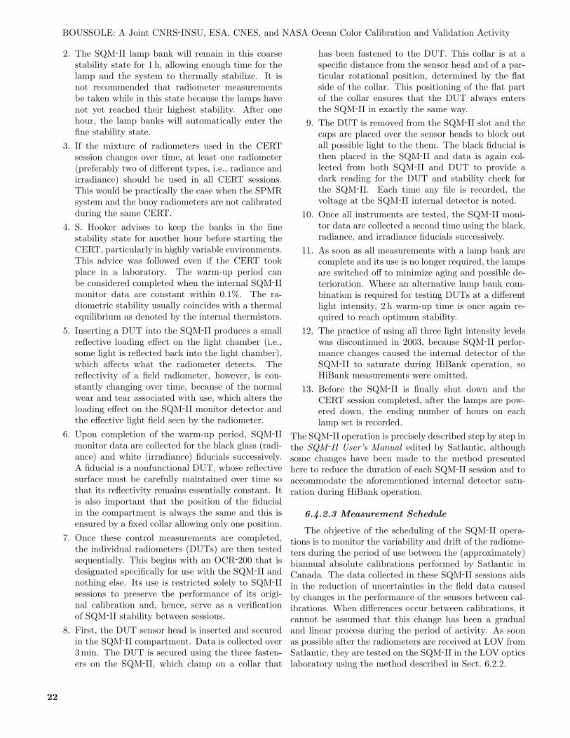
BOUSSOLE: A Joint CNRS-INSU, ESA, CNES, and NASA Ocean Color Calibration and Validation Activity
2. The SQM-II lamp bank will remain in this coarsestability state for 1 h, allowing enough time for thelamp and the system to thermally stabilize. It isnot recommended that radiometer measurementsbe taken while in this state because the lamps havenot yet reached their highest stability. After onehour, the lamp banks will automatically enter thefine stability state.
3. If the mixture of radiometers used in the CERTsession changes over time, at least one radiometer(preferably two of different types, i.e., radiance andirradiance) should be used in all CERT sessions.This would be practically the case when the SPMRsystem and the buoy radiometers are not calibratedduring the same CERT.
4. S. Hooker advises to keep the banks in the finestability state for another hour before starting theCERT, particularly in highly variable environments.This advice was followed even if the CERT tookplace in a laboratory. The warm-up period canbe considered completed when the internal SQM-IImonitor data are constant within 0.1%. The ra-diometric stability usually coincides with a thermalequilibrium as denoted by the internal thermistors.
5. Inserting a DUT into the SQM-II produces a smallreflective loading effect on the light chamber (i.e.,some light is reflected back into the light chamber),which affects what the radiometer detects. Thereflectivity of a field radiometer, however, is con-stantly changing over time, because of the normalwear and tear associated with use, which alters theloading effect on the SQM-II monitor detector andthe effective light field seen by the radiometer.
6. Upon completion of the warm-up period, SQM-IImonitor data are collected for the black glass (radi-ance) and white (irradiance) fiducials successively.A fiducial is a nonfunctional DUT, whose reflectivesurface must be carefully maintained over time sothat its reflectivity remains essentially constant. Itis also important that the position of the fiducialin the compartment is always the same and this isensured by a fixed collar allowing only one position.
7. Once these control measurements are completed,the individual radiometers (DUTs) are then testedsequentially. This begins with an OCR-200 that isdesignated specifically for use with the SQM-II andnothing else. Its use is restricted solely to SQM-IIsessions to preserve the performance of its origi-nal calibration and, hence, serve as a verificationof SQM-II stability between sessions.
8. First, the DUT sensor head is inserted and securedin the SQM-II compartment. Data is collected over3 min. The DUT is secured using the three fasten-ers on the SQM-II, which clamp on a collar that
has been fastened to the DUT. This collar is at aspecific distance from the sensor head and of a par-ticular rotational position, determined by the flatside of the collar. This positioning of the flat partof the collar ensures that the DUT always entersthe SQM-II in exactly the same way.
9. The DUT is removed from the SQM-II slot and thecaps are placed over the sensor heads to block outall possible light to the them. The black fiducial isthen placed in the SQM-II and data is again col-lected from both SQM-II and DUT to provide adark reading for the DUT and stability check forthe SQM-II. Each time any file is recorded, thevoltage at the SQM-II internal detector is noted.
10. Once all instruments are tested, the SQM-II moni-tor data are collected a second time using the black,radiance, and irradiance fiducials successively.
11. As soon as all measurements with a lamp bank arecomplete and its use is no longer required, the lampsare switched off to minimize aging and possible de-terioration. Where an alternative lamp bank com-bination is required for testing DUTs at a differentlight intensity, 2 h warm-up time is once again re-quired to reach optimum stability.
12. The practice of using all three light intensity levelswas discontinued in 2003, because SQM-II perfor-mance changes caused the internal detector of theSQM-II to saturate during HiBank operation, soHiBank measurements were omitted.
13. Before the SQM-II is finally shut down and theCERT session completed, after the lamps are pow-ered down, the ending number of hours on eachlamp set is recorded.
The SQM-II operation is precisely described step by step inthe SQM-II User’s Manual edited by Satlantic, althoughsome changes have been made to the method presentedhere to reduce the duration of each SQM-II session and toaccommodate the aforementioned internal detector satu-ration during HiBank operation.
6.4.2.3 Measurement Schedule
The objective of the scheduling of the SQM-II opera-tions is to monitor the variability and drift of the radiome-ters during the period of use between the (approximately)biannual absolute calibrations performed by Satlantic inCanada. The data collected in these SQM-II sessions aidsin the reduction of uncertainties in the field data causedby changes in the performance of the sensors between cal-ibrations. When differences occur between calibrations, itcannot be assumed that this change has been a gradualand linear process during the period of activity. As soonas possible after the radiometers are received at LOV fromSatlantic, they are tested on the SQM-II in the LOV opticslaboratory using the method described in Sect. 6.2.2.
22
Antoine et al.
Once the sensors have been used in the field, eitherfixed on the buoy or profiled from the ship, they are sub-jected to testing on the SQM-II. The exact scheduling ofthis testing depends on the duration of the field work. Forthe buoy radiometers, which are intended to be exchangedon a monthly basis, the SQM-II session is performed assoon as possible after they have been taken off the buoyand returned to the lab (once they have been wiped downwith soapy water and a soft cloth). For the SPMR andSMSR, the SQM-II session is performed after each cruise.
6.4.3 Immersion Factors
The eighth SeaWiFS Intercalibration Round-Robin Ex-periment (SIRREX-8) conclusively demonstrated that im-mersion factors must be determined for each sensor if aless than 3% the uncertainty in irradiance determinationsis to be achieved (Zibordi et al. 2002b). A water tankbased on the Hooker and Zibordi (2005) design—the socalled Compact Portable Advanced Characterization Tank(ComPACT)—was developed and is used for characteriz-ing buoy radiometers.
The objective here is to determine specific sets of co-efficients for the radiometers, and, more importantly, tocheck whether these coefficients are changing over timebecause of their prolonged deployments at sea. For themoment, the results of these experiments do not showappreciable changes, although confirmation by additionalmeasurements is still pending. More definitive conclusionsalso depend on future improvements in the reproducibilityof the experiments, in order to meet the requested perfor-mance levels (Hooker and Zibordi 2005).
6.5 Bio-FoulingBio-fouling is a critical aspect of mooring applications.
The development of new systems for preventing bio-fouling(chemicals or mechanisms) has not been considered in theproject, at least up to now. Minimizing bio-fouling oninstruments first requires that the structure they are in-stalled on is kept clean. When the mounting structure isbio-fouled, algal growth restarts more rapidly after the in-struments are cleaned, so an effective antifouling paint onthe buoy superstructure is required.
Concerning the radiometers, the quality of their mea-surements is preserved by the following ways:
Copper sheets have been added around the radiome-ters’ bodies (since June 2005).The sensors are cleaned during each monthly main-tenance visit by divers equipped with brushes (sinceJuly 2006, the cleaning has been performed approx-imately every two weeks).Diffusers or filters are replaced if the absolute cal-ibration indicates it is timely to do so. This oper-ation can be performed after the upper superstruc-ture rotations, which occur about twice a year.
Glass windows of the radiance sensors are kept asclean and smooth as possible, which is the best an-tifouling procedure following McLean et al. (1997).
The above procedures are considered sufficient, at leastas a first approach, especially given the oligotrophic-to-mesotrophic character of the mooring site. The cleaningof the radiometers every two weeks is the central elementin the strategy to eliminate bio-fouling effects from themeasurements of radiometric quantities. Concerning thetransmissometers, copper rings have been installed aroundthe emission and reception windows. A copper face platehas been installed onto the Hydroscat-II.
All the above devices and procedures have proven to beefficient but cannot totally eliminate bio-fouling, so thatcorrections for possible residual effects will have to be ap-plied. The total effect of bio-fouling, which can be de-termined from the comparison of the measurements takenjust before and just after cleaning of the sensors, will haveto be distributed over time in some manner.
7. DATA ANALYSISData analyses procedures are summarized in the follow-
ing six subsections. This part is not meant to be exhaus-tive; only the analyses considered as the most importantare presented.
7.1 HPLCThe methods described here were evaluated as part
of three international SeaWiFS HPLC Analysis Round-Robin Experiment (SeaHARRE) exercises: SeaHARRE-1(Hooker et al. 2000), SeaHARRE-2 (Hooker et al. 2005)and SeaHARRE-3 (Hooker et al. 2007). The round robinswere based on both natural samples and standard mixturesrepresenting a wide range of Chl a concentrations fromthe hyper-oligotrophic conditions of the Mediterranean Seaand South Pacific Gyre to the very eutrophic waters of theBenguela, Moroccan, and Chilean upwelling systems. Fourto eight laboratories from seven countries have taken partin these activities.
As a result of these exercises, the LOV has demon-strated that satisfactory results are provided for the anal-ysis of Chl a and accessory pigments in seawater samplesfrom different concentration regimes: the method used un-dergoes detailed quality control procedures, and a series ofvalidation parameters are regularly monitored in order toensure a good continuity in the data.
7.1.1 Sample Collection
Seawater samples were collected from Niskin bottlesand filtered through 25 mm GF/F Whatman filters (0.7µmporosity). In most cases, 2.8 L were filtered for each sam-ple and the filters were placed in Petri slides, wrapped inaluminium and stored first in liquid nitrogen on board andthen in a −80◦C freezer in the laboratory.
23
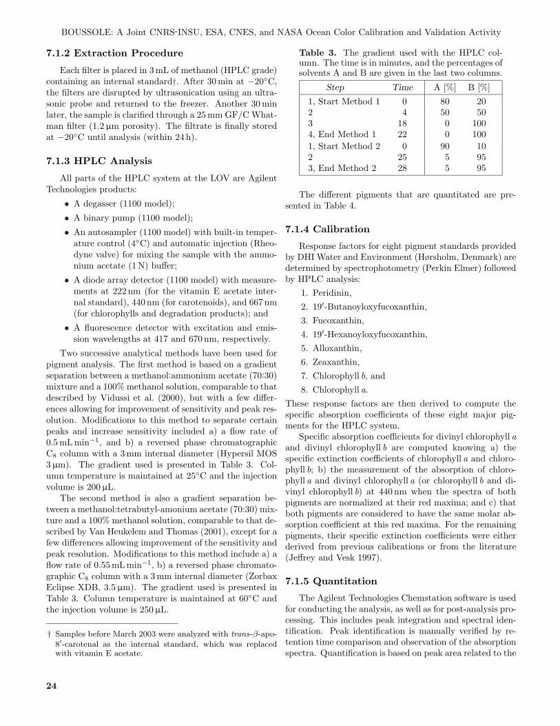
BOUSSOLE: A Joint CNRS-INSU, ESA, CNES, and NASA Ocean Color Calibration and Validation Activity
7.1.2 Extraction Procedure
Each filter is placed in 3 mL of methanol (HPLC grade)containing an internal standard†. After 30 min at −20◦C,the filters are disrupted by ultrasonication using an ultra-sonic probe and returned to the freezer. Another 30 minlater, the sample is clarified through a 25 mm GF/C What-man filter (1.2µm porosity). The filtrate is finally storedat −20◦C until analysis (within 24 h).
7.1.3 HPLC Analysis
All parts of the HPLC system at the LOV are AgilentTechnologies products:
• A degasser (1100 model);
• A binary pump (1100 model);
• An autosampler (1100 model) with built-in temper-ature control (4◦C) and automatic injection (Rheo-dyne valve) for mixing the sample with the ammo-nium acetate (1 N) buffer;
• A diode array detector (1100 model) with measure-ments at 222 nm (for the vitamin E acetate inter-nal standard), 440 nm (for carotenoids), and 667 nm(for chlorophylls and degradation products); and
• A fluorescence detector with excitation and emis-sion wavelengths at 417 and 670 nm, respectively.
Two successive analytical methods have been used forpigment analysis. The first method is based on a gradientseparation between a methanol:ammonium acetate (70:30)mixture and a 100% methanol solution, comparable to thatdescribed by Vidussi et al. (2000), but with a few differ-ences allowing for improvement of sensitivity and peak res-olution. Modifications to this method to separate certainpeaks and increase sensitivity included a) a flow rate of0.5 mL min−1, and b) a reversed phase chromatographicC8 column with a 3 mm internal diameter (Hypersil MOS3 µm). The gradient used is presented in Table 3. Col-umn temperature is maintained at 25◦C and the injectionvolume is 200 µL.
The second method is also a gradient separation be-tween a methanol:tetrabutyl-amonium acetate (70:30) mix-ture and a 100% methanol solution, comparable to that de-scribed by Van Heukelem and Thomas (2001), except for afew differences allowing improvement of the sensitivity andpeak resolution. Modifications to this method include a) aflow rate of 0.55 mL min−1, b) a reversed phase chromato-graphic C8 column with a 3 mm internal diameter (ZorbaxEclipse XDB, 3.5 µm). The gradient used is presented inTable 3. Column temperature is maintained at 60◦C andthe injection volume is 250µL.
† Samples before March 2003 were analyzed with trans-β-apo-8′-carotenal as the internal standard, which was replacedwith vitamin E acetate.
Table 3. The gradient used with the HPLC col-umn. The time is in minutes, and the percentages ofsolvents A and B are given in the last two columns.
Step Time A [%] B [%]
1, Start Method 1 0 80 202 4 50 503 18 0 1004, End Method 1 22 0 1001, Start Method 2 0 90 102 25 5 953, End Method 2 28 5 95
The different pigments that are quantitated are pre-sented in Table 4.
7.1.4 Calibration
Response factors for eight pigment standards providedby DHI Water and Environment (Hørsholm, Denmark) aredetermined by spectrophotometry (Perkin Elmer) followedby HPLC analysis:
1. Peridinin,2. 19′-Butanoyloxyfucoxanthin,3. Fucoxanthin,4. 19′-Hexanoyloxyfucoxanthin,5. Alloxanthin,6. Zeaxanthin,7. Chlorophyll b, and8. Chlorophyll a.
These response factors are then derived to compute thespecific absorption coefficients of these eight major pig-ments for the HPLC system.
Specific absorption coefficients for divinyl chlorophyll aand divinyl chlorophyll b are computed knowing a) thespecific extinction coefficients of chlorophyll a and chloro-phyll b; b) the measurement of the absorption of chloro-phyll a and divinyl chlorophyll a (or chlorophyll b and di-vinyl chlorophyll b) at 440 nm when the spectra of bothpigments are normalized at their red maxima; and c) thatboth pigments are considered to have the same molar ab-sorption coefficient at this red maxima. For the remainingpigments, their specific extinction coefficients were eitherderived from previous calibrations or from the literature(Jeffrey and Vesk 1997).
7.1.5 Quantitation
The Agilent Technologies Chemstation software is usedfor conducting the analysis, as well as for post-analysis pro-cessing. This includes peak integration and spectral iden-tification. Peak identification is manually verified by re-tention time comparison and observation of the absorptionspectra. Quantification is based on peak area related to the
24
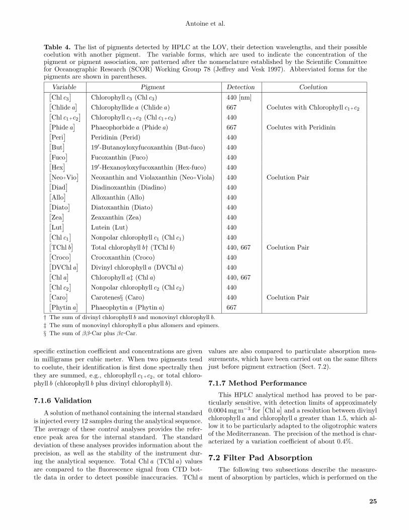
Antoine et al.
Table 4. The list of pigments detected by HPLC at the LOV, their detection wavelengths, and their possiblecoelution with another pigment. The variable forms, which are used to indicate the concentration of thepigment or pigment association, are patterned after the nomenclature established by the Scientific Committeefor Oceanographic Research (SCOR) Working Group 78 (Jeffrey and Vesk 1997). Abbreviated forms for thepigments are shown in parentheses.
Variable Pigment Detection Coelution[Chl c3
]Chlorophyll c3 (Chl c3) 440 [nm][
Chlide a]
Chlorophyllide a (Chlide a) 667 Coelutes with Chlorophyll c1+c2[Chl c1+c2
]Chlorophyll c1+c2 (Chl c1+c2) 440[
Phide a]
Phaeophorbide a (Phide a) 667 Coelutes with Peridinin[Peri
]Peridinin (Perid) 440[
But]
19′-Butanoyloxyfucoxanthin (But-fuco) 440[Fuco
]Fucoxanthin (Fuco) 440[
Hex]
19′-Hexanoyloxyfucoxanthin (Hex-fuco) 440[Neo+Vio
]Neoxanthin and Violaxanthin (Neo+Viola) 440 Coelution Pair[
Diad]
Diadinoxanthin (Diadino) 440[Allo
]Alloxanthin (Allo) 440[
Diato]
Diatoxanthin (Diato) 440[Zea
]Zeaxanthin (Zea) 440[
Lut]
Lutein (Lut) 440[Chl c1
]Nonpolar chlorophyll c1 (Chl c1) 440[
TChl b]
Total chlorophyll b† (TChl b) 440, 667 Coelution Pair[Croco
]Crocoxanthin (Croco) 440[
DVChl a]
Divinyl chlorophyll a (DVChl a) 440[Chl a
]Chlorophyll a‡ (Chl a) 440, 667[
Chl c2
]Nonpolar chlorophyll c2 (Chl c2) 440[
Caro]
Carotenes§ (Caro) 440 Coelution Pair[Phytin a
]Phaeophytin a (Phytin a) 667
† The sum of divinyl chlorophyll b and monovinyl chlorophyll b.
‡ The sum of monovinyl chlorophyll a plus allomers and epimers.
§ The sum of ββ-Car plus βε-Car.
specific extinction coefficient and concentrations are givenin milligrams per cubic meter. When two pigments tendto coelute, their identification is first done spectrally thenthey are summed, e.g., chlorophyll c1+c2, or total chloro-phyll b (chlorophyll b plus divinyl chlorophyll b).
7.1.6 Validation
A solution of methanol containing the internal standardis injected every 12 samples during the analytical sequence.The average of these control analyses provides the refer-ence peak area for the internal standard. The standarddeviation of these analyses provides information about theprecision, as well as the stability of the instrument dur-ing the analytical sequence. Total Chl a (TChl a) valuesare compared to the fluorescence signal from CTD bot-tle data in order to detect possible inaccuracies. TChl a
values are also compared to particulate absorption mea-surements, which have been carried out on the same filtersjust before pigment extraction (Sect. 7.2).
7.1.7 Method Performance
This HPLC analytical method has proved to be par-ticularly sensitive, with detection limits of approximately0.0004 mg m−3 for
[Chl a
]and a resolution between divinyl
chlorophyll a and chlorophyll a greater than 1.5, which al-low it to be particularly adapted to the oligotrophic watersof the Mediterranean. The precision of the method is char-acterized by a variation coefficient of about 0.4%.
7.2 Filter Pad AbsorptionThe following two subsections describe the measure-
ment of absorption by particles, which is performed on the
25

BOUSSOLE: A Joint CNRS-INSU, ESA, CNES, and NASA Ocean Color Calibration and Validation Activity
same filter that is subsequently used for the HPLC pigmentanalysis previously described.
7.2.1 Laboratory Analyses
The protocol for analyzing the spectral absorption co-efficients of particulates is based on the NASA Ocean Op-tics Protocols for Satellite Ocean Color Sensor Validation(Mitchell et al. 2003). Sampling is performed in the sameway as for the HPLC pigments as described in Sect. 8.1where the seawater samples are collected from Niskin bot-tles and filtered through 25 mm GF/F Whatman filters(0.7µm porosity). In most cases, 2.8 L are filtered for eachsample and the filters placed in petri slides, wrapped inaluminum foil and stored first in liquid nitrogen on board,and then in a −80◦C freezer in the laboratory. The samplefilters used for the Ap analysis are also used afterwards forHPLC analysis. This method has been tested to ensurethat using the same filter for the two methods does notcompromise either measure.
The spectrophotometer used is a Perkin Elmer Lambda19 (L19) dual-path spectrometer with an integrating spherecompartment attached. The instrument scan range is setfrom 750–350 nm with a scan interval of 1 nm. After a 1 hwarm-up period, the machine is ready to use. The samplesare taken out of the −80◦C freezer and stored temporarilyin an ice-cooled cold box. Each sample, in its petri dish, isthen placed in a dark box on the bench to defrost for 5 min.This defrosting period is kept to a minimum because thepigment composition once thawed becomes susceptible todegradation which could effect the analyses, particularlythe HPLC.
The L19, being a dual-path spectrometer, has a slotfor a reference material and another for the sample. Theseslots are actually the outer walls of the integrating sphereat the two positions where the two beams enter the sphere.For the reference path, rather than use a blank filter, whichcan create variations in the spectra attributable to differ-ences in the level of moistness of the filter, the pathwayis left open (without any filter blank), thus using an airblank. In the sample material slot, a blank GF/F filteris used. This blank has been soaked in distilled water for12 h and had excess water drained off before being placedin the sample slot.
An autozero is performed with the blank filter in thesample path and the reference path open, which sets theabsorbance values measured at each wavelength to zero.As a verification of this and to provide a baseline, the blankis then scanned to measure absorbance. The spectra pro-duced from this should be flat and close to zero (within0.005). If this is not the case, the autozero is repeated andthe blanks scanned again.
Once satisfactory baselines are achieved, then the sam-ple filters can be scanned. For both cases, two scans aremade, which should produce two similar replicates. If sim-ilarity is not found, the filter position is checked and the
sample scanned again. Drying of the filter between repli-cates may cause some vertical offsetting, which is accept-able if the spectral shape for each replicate is similar.
The spectra are saved as a file in American StandardCode for Information Interchange (ASCII) format with twocolumns: wavelength and absorbance. The mean of the ab-sorbance values of replicates for each sample is calculatedand any offset from zero removed by subtracting the ab-sorbance value at 750 nm from the entire spectrum.
7.2.2 Data Postprocessing
The optical densities are then corrected for any nonzerosignal in the NIR (750 nm), and transformed into absorp-tion coefficients by accounting for the so-called β effect.The total particulate absorption spectra are then numeri-cally decomposed into a phytoplankton and a detritus ab-sorption spectra following Bricaud and Stramski (1990).
7.3 Total Suspended Matter (TSM)TSM is determined with a gravimetric method based on
the protocol described by Strickland and Parsons (1972).Before sampling, 25 mm diameter Whatman GF/F glassfiber filters (0.7µm particle retention size) are pre-rinsedin methanol, pre-combusted at 450◦C for 4 h, and pre-weighed to six significant digits with a Metler-Toledo elec-trobalance (ambient temperature and humidity are alsorecorded).
In the field, 1.5–5.6 L seawater samples (the chosen vol-ume depends on the amount of material in the water) frombelow the surface are collected in triplicate using vacuumfiltration. The filters and filter-rims are rinsed with 20–30 mL of milli-Q water in order to eliminate the presenceof salt crystals. They are placed in polycarbonate petridishes and stored in liquid nitrogen and at −80◦C until lab-oratory analysis. The filters are dried in an oven at 75◦Cfor 24 h and placed in a dessicator before being weighed tosix digits of precision (ambient temperature and humid-ity are recorded). The TSM is calculated as the differencebetween the sample weight minus the weight before filtra-tion (in grams), and then divided by the filtration volumein cubic meters (concentrations are, therefore, grams percubic meter).
7.4 AC-9 and ECO-BB3 Data ProcessingWhen a CTD cast is performed, the CTD and AC-9+
start times are not synchronized. In addition, each in-strument has a specific time constant and the water cir-culation in the tubing generates additional temporal off-sets. In order to account for these time lags, the verti-cal profiles for absorption and attenuation must be shiftedin order to match the vertical profiles of other data suchas the chlorophyll fluorescence and the temperature. Thematching is either performed manually using clearly iden-tifiable features in the profiles (i.e., peaks) or automati-cally when the time lag between the start of the various
26
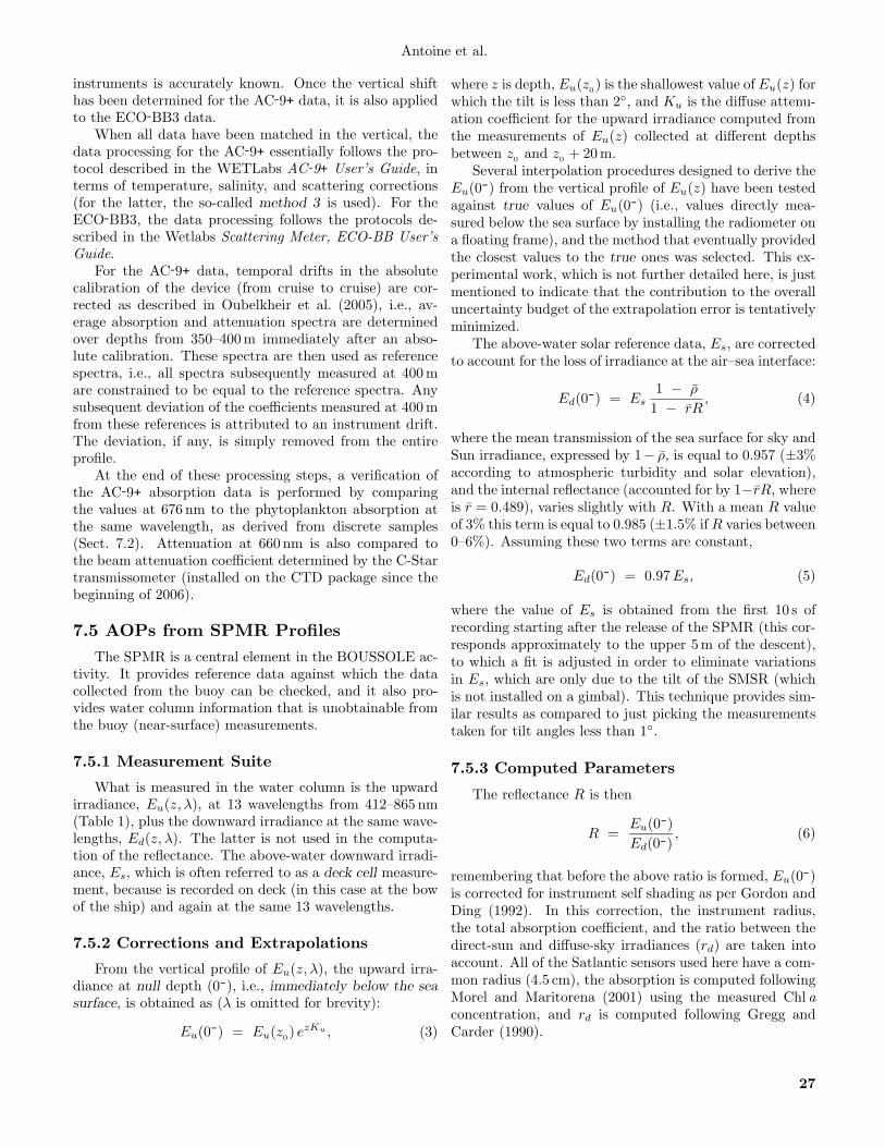
Antoine et al.
instruments is accurately known. Once the vertical shifthas been determined for the AC-9+ data, it is also appliedto the ECO-BB3 data.
When all data have been matched in the vertical, thedata processing for the AC-9+ essentially follows the pro-tocol described in the WETLabs AC-9+ User’s Guide, interms of temperature, salinity, and scattering corrections(for the latter, the so-called method 3 is used). For theECO-BB3, the data processing follows the protocols de-scribed in the Wetlabs Scattering Meter, ECO-BB User’sGuide.
For the AC-9+ data, temporal drifts in the absolutecalibration of the device (from cruise to cruise) are cor-rected as described in Oubelkheir et al. (2005), i.e., av-erage absorption and attenuation spectra are determinedover depths from 350–400 m immediately after an abso-lute calibration. These spectra are then used as referencespectra, i.e., all spectra subsequently measured at 400 mare constrained to be equal to the reference spectra. Anysubsequent deviation of the coefficients measured at 400 mfrom these references is attributed to an instrument drift.The deviation, if any, is simply removed from the entireprofile.
At the end of these processing steps, a verification ofthe AC-9+ absorption data is performed by comparingthe values at 676 nm to the phytoplankton absorption atthe same wavelength, as derived from discrete samples(Sect. 7.2). Attenuation at 660 nm is also compared tothe beam attenuation coefficient determined by the C-Startransmissometer (installed on the CTD package since thebeginning of 2006).
7.5 AOPs from SPMR ProfilesThe SPMR is a central element in the BOUSSOLE ac-
tivity. It provides reference data against which the datacollected from the buoy can be checked, and it also pro-vides water column information that is unobtainable fromthe buoy (near-surface) measurements.
7.5.1 Measurement Suite
What is measured in the water column is the upwardirradiance, Eu(z, λ), at 13 wavelengths from 412–865 nm(Table 1), plus the downward irradiance at the same wave-lengths, Ed(z, λ). The latter is not used in the computa-tion of the reflectance. The above-water downward irradi-ance, Es, which is often referred to as a deck cell measure-ment, because is recorded on deck (in this case at the bowof the ship) and again at the same 13 wavelengths.
7.5.2 Corrections and Extrapolations
From the vertical profile of Eu(z, λ), the upward irra-diance at null depth (0-), i.e., immediately below the seasurface, is obtained as (λ is omitted for brevity):
Eu(0-) = Eu(z0) ezKu , (3)
where z is depth, Eu(z0) is the shallowest value of Eu(z) forwhich the tilt is less than 2◦, and Ku is the diffuse attenu-ation coefficient for the upward irradiance computed fromthe measurements of Eu(z) collected at different depthsbetween z0 and z0 + 20 m.
Several interpolation procedures designed to derive theEu(0-) from the vertical profile of Eu(z) have been testedagainst true values of Eu(0-) (i.e., values directly mea-sured below the sea surface by installing the radiometer ona floating frame), and the method that eventually providedthe closest values to the true ones was selected. This ex-perimental work, which is not further detailed here, is justmentioned to indicate that the contribution to the overalluncertainty budget of the extrapolation error is tentativelyminimized.
The above-water solar reference data, Es, are correctedto account for the loss of irradiance at the air–sea interface:
Ed(0-) = Es1 − ρ
1 − rR, (4)
where the mean transmission of the sea surface for sky andSun irradiance, expressed by 1− ρ, is equal to 0.957 (±3%according to atmospheric turbidity and solar elevation),and the internal reflectance (accounted for by 1−rR, whereis r = 0.489), varies slightly with R. With a mean R valueof 3% this term is equal to 0.985 (±1.5% if R varies between0–6%). Assuming these two terms are constant,
Ed(0-) = 0.97 Es, (5)
where the value of Es is obtained from the first 10 s ofrecording starting after the release of the SPMR (this cor-responds approximately to the upper 5 m of the descent),to which a fit is adjusted in order to eliminate variationsin Es, which are only due to the tilt of the SMSR (whichis not installed on a gimbal). This technique provides sim-ilar results as compared to just picking the measurementstaken for tilt angles less than 1◦.
7.5.3 Computed Parameters
The reflectance R is then
R =Eu(0-)Ed(0-)
, (6)
remembering that before the above ratio is formed, Eu(0-)is corrected for instrument self shading as per Gordon andDing (1992). In this correction, the instrument radius,the total absorption coefficient, and the ratio between thedirect-sun and diffuse-sky irradiances (rd) are taken intoaccount. All of the Satlantic sensors used here have a com-mon radius (4.5 cm), the absorption is computed followingMorel and Maritorena (2001) using the measured Chl aconcentration, and rd is computed following Gregg andCarder (1990).
27
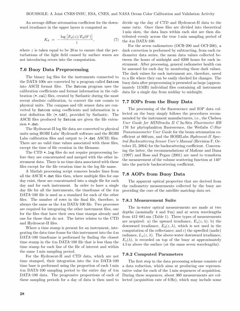
BOUSSOLE: A Joint CNRS-INSU, ESA, CNES, and NASA Ocean Color Calibration and Validation Activity
An average diffuse attenuation coefficient for the down-ward irradiance in the upper layers is computed as
Kd = − log[Ed(z)/Ed(0-)
]z
, (7)
where z is taken equal to be 20 m to ensure that the per-turbations of the light field caused by surface waves arenot introducing errors into the computation.
7.6 Buoy Data Preprocessing
The binary log files for the instruments connected tothe DATA-100s are converted by a program called Satconinto ASCII format files. The Satcon program uses thecalibration coefficients and format information in the cali-bration (*.cal) files, created by Satlantic during the mostrecent absolute calibration, to convert the raw counts tophysical units. The compass and tilt sensor data are con-verted by Satcon using coefficients and information in atext definition file (*.tdf), provided by Satlantic. TheASCII files produced by Satcon are given the file exten-sion *.dat.
The Hydroscat-II log file data are converted to physicalunits using HOBI Labs’ Hydrosoft software and the HOBILabs calibration files and output to (*.dat ASCII) files.There are no valid time values associated with these files,except the time of file creation in the filename.
The CTD *.log files do not require preprocessing be-fore they are concatenated and merged with the other in-strument data. There is no time data associated with thesefiles except for the file creation time in the log file name.
A Matlab processing script removes header lines fromall the ASCII *.dat files then, where multiple files for oneday exist, these are concatenated into a single file for eachday and for each instrument. In order to have a singleday file for all the instruments, the timeframe of the 4 mDATA-100 file is used as a standard for each of the otherfiles. The number of rows in the final file, therefore, isalways the same as the 4 m DATA-100 file. Two processesare required for integrating the other instrument files, onefor the files that have their own time stamps already andone for those that do not. The latter relates to the CTDand Hydroscat-II files.
Where a time stamp is present for an instrument, inte-grating the data time frame for this instrument into the 4 mDATA-100 timeframe is performed by finding the closesttime stamp in the 4 m DATA-100 file that is less than thetime stamp for each line of the file of interest and withinthe same 1 min sampling period.
For the Hydroscat-II and CTD data, which are nottime stamped, their integration into the 4 m DATA-100time base is performed using the proportion of each 1 min4 m DATA-100 sampling period to the entire day of 4 mDATA-100 data. The progressive proportions of each ofthese sampling periods for a day of data is then used to
divide up the day of CTD and Hydroscat-II data to thesame ratio. Once these files are divided into theoretical1 min slots, the data lines within each slot are then dis-tributed evenly across the true 1 min sampling period ofthe 4 m DATA-100.
For the seven radiometers (OCR-200 and OCI-200), adark correction is performed by subtracting, from each ra-diometer data series, the mean data values collected be-tween the hours of midnight and 0200 hours for each in-strument. After processing, general radiometer health canbe assessed for each day by monitoring these dark values.The dark values for each instrument are, therefore, savedto a file where they can be easily checked for changes. Thebuoy data after preprocessing is presented as large (approx-imately 13 MB) individual files containing all instrumentdata for a single day from midday to midnight.
7.7 IOPs from the Buoy DataThe processing of the fluorescence and IOP data col-
lected on the buoy simply follows the procedures recom-mended by the instrument manufacturers, i.e., the ChelseaUser Guide for MINItracka II C In-Situ Fluorimeter HB176 for phytoplankton fluorescence, the Wetlabs C-StarTransmissometer User Guide for the beam attenuation co-efficient at 660 nm, and the HOBILabs Hydroscat-II Spec-tral Backscattering Sensor User’s Manual (Revision F, Oc-tober 25, 2004) for the backscattering coefficient. Concern-ing the latter, the recommendations of Mafione and Dana(1997) and Boss and Pegau (2001) are used to transformthe measurement of the volume scattering function at 140◦
into the particle backscattering coefficient.
7.8 AOPs from Buoy DataThe apparent optical properties that are derived from
the radiometry measurements collected by the buoy areproviding the core of the satellite matchup data set.
7.8.1 Measurement Suite
The in-water optical measurements are made at twodepths (nominally 4 and 9 m) and at seven wavelengthsfrom 412–681 nm (Table 1). Three types of measurementsare acquired: a) the upward irradiance, Eu(z, λ); b) thedownward irradiance, Ed(z, λ), which is not used in thecomputation of the reflectance; and c) the upwelled (nadir)radiance, Lu(z, λ). The above-water downward irradiance,Es(λ), is recorded on top of the buoy at approximately4.5 m above the surface (at the same seven wavelengths).
7.8.2 Computed Parameters
The first step in the data processing scheme consists ofa data reduction, which aims at producing one represen-tative value for each of the 1 min sequences of acquisition.During these sequences, about 360 measurements are col-lected (acquisition rate of 6 Hz), which may include some
28
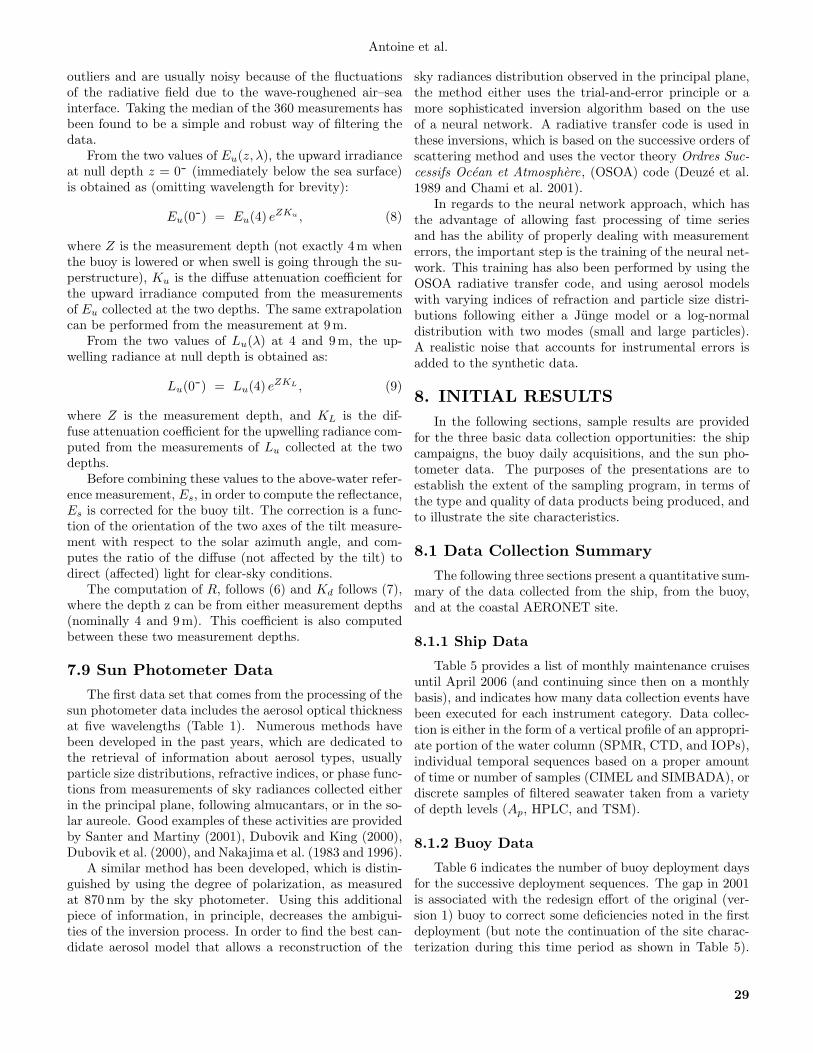
Antoine et al.
outliers and are usually noisy because of the fluctuationsof the radiative field due to the wave-roughened air–seainterface. Taking the median of the 360 measurements hasbeen found to be a simple and robust way of filtering thedata.
From the two values of Eu(z, λ), the upward irradianceat null depth z = 0- (immediately below the sea surface)is obtained as (omitting wavelength for brevity):
Eu(0-) = Eu(4) eZKu , (8)
where Z is the measurement depth (not exactly 4 m whenthe buoy is lowered or when swell is going through the su-perstructure), Ku is the diffuse attenuation coefficient forthe upward irradiance computed from the measurementsof Eu collected at the two depths. The same extrapolationcan be performed from the measurement at 9 m.
From the two values of Lu(λ) at 4 and 9 m, the up-welling radiance at null depth is obtained as:
Lu(0-) = Lu(4) eZKL , (9)
where Z is the measurement depth, and KL is the dif-fuse attenuation coefficient for the upwelling radiance com-puted from the measurements of Lu collected at the twodepths.
Before combining these values to the above-water refer-ence measurement, Es, in order to compute the reflectance,Es is corrected for the buoy tilt. The correction is a func-tion of the orientation of the two axes of the tilt measure-ment with respect to the solar azimuth angle, and com-putes the ratio of the diffuse (not affected by the tilt) todirect (affected) light for clear-sky conditions.
The computation of R, follows (6) and Kd follows (7),where the depth z can be from either measurement depths(nominally 4 and 9 m). This coefficient is also computedbetween these two measurement depths.
7.9 Sun Photometer DataThe first data set that comes from the processing of the
sun photometer data includes the aerosol optical thicknessat five wavelengths (Table 1). Numerous methods havebeen developed in the past years, which are dedicated tothe retrieval of information about aerosol types, usuallyparticle size distributions, refractive indices, or phase func-tions from measurements of sky radiances collected eitherin the principal plane, following almucantars, or in the so-lar aureole. Good examples of these activities are providedby Santer and Martiny (2001), Dubovik and King (2000),Dubovik et al. (2000), and Nakajima et al. (1983 and 1996).
A similar method has been developed, which is distin-guished by using the degree of polarization, as measuredat 870 nm by the sky photometer. Using this additionalpiece of information, in principle, decreases the ambigui-ties of the inversion process. In order to find the best can-didate aerosol model that allows a reconstruction of the
sky radiances distribution observed in the principal plane,the method either uses the trial-and-error principle or amore sophisticated inversion algorithm based on the useof a neural network. A radiative transfer code is used inthese inversions, which is based on the successive orders ofscattering method and uses the vector theory Ordres Suc-cessifs Ocean et Atmosphere, (OSOA) code (Deuze et al.1989 and Chami et al. 2001).
In regards to the neural network approach, which hasthe advantage of allowing fast processing of time seriesand has the ability of properly dealing with measurementerrors, the important step is the training of the neural net-work. This training has also been performed by using theOSOA radiative transfer code, and using aerosol modelswith varying indices of refraction and particle size distri-butions following either a Junge model or a log-normaldistribution with two modes (small and large particles).A realistic noise that accounts for instrumental errors isadded to the synthetic data.
8. INITIAL RESULTSIn the following sections, sample results are provided
for the three basic data collection opportunities: the shipcampaigns, the buoy daily acquisitions, and the sun pho-tometer data. The purposes of the presentations are toestablish the extent of the sampling program, in terms ofthe type and quality of data products being produced, andto illustrate the site characteristics.
8.1 Data Collection Summary
The following three sections present a quantitative sum-mary of the data collected from the ship, from the buoy,and at the coastal AERONET site.
8.1.1 Ship Data
Table 5 provides a list of monthly maintenance cruisesuntil April 2006 (and continuing since then on a monthlybasis), and indicates how many data collection events havebeen executed for each instrument category. Data collec-tion is either in the form of a vertical profile of an appropri-ate portion of the water column (SPMR, CTD, and IOPs),individual temporal sequences based on a proper amountof time or number of samples (CIMEL and SIMBADA), ordiscrete samples of filtered seawater taken from a varietyof depth levels (Ap, HPLC, and TSM).
8.1.2 Buoy Data
Table 6 indicates the number of buoy deployment daysfor the successive deployment sequences. The gap in 2001is associated with the redesign effort of the original (ver-sion 1) buoy to correct some deficiencies noted in the firstdeployment (but note the continuation of the site charac-terization during this time period as shown in Table 5).
29
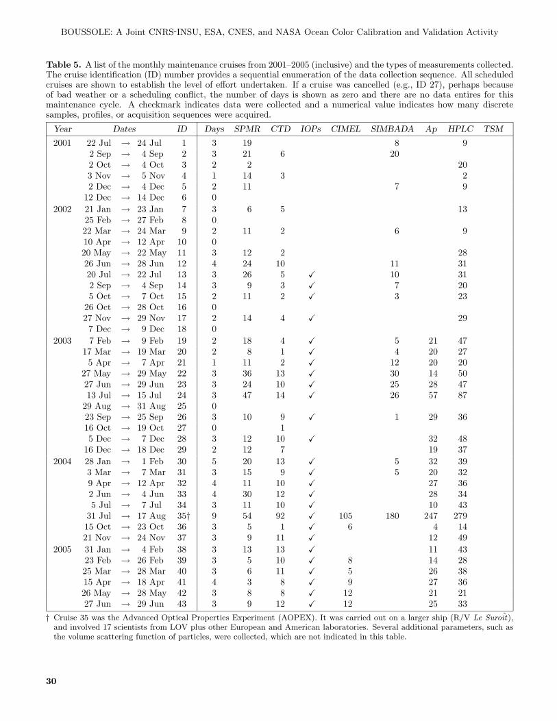
BOUSSOLE: A Joint CNRS-INSU, ESA, CNES, and NASA Ocean Color Calibration and Validation Activity
Table 5. A list of the monthly maintenance cruises from 2001–2005 (inclusive) and the types of measurements collected.The cruise identification (ID) number provides a sequential enumeration of the data collection sequence. All scheduledcruises are shown to establish the level of effort undertaken. If a cruise was cancelled (e.g., ID 27), perhaps becauseof bad weather or a scheduling conflict, the number of days is shown as zero and there are no data entires for thismaintenance cycle. A checkmark indicates data were collected and a numerical value indicates how many discretesamples, profiles, or acquisition sequences were acquired.
Year Dates ID Days SPMR CTD IOPs CIMEL SIMBADA Ap HPLC TSM
2001 22 Jul → 24 Jul 1 3 19 8 92 Sep → 4 Sep 2 3 21 6 202 Oct → 4 Oct 3 2 2 203 Nov → 5 Nov 4 1 14 3 22 Dec → 4 Dec 5 2 11 7 9
12 Dec → 14 Dec 6 02002 21 Jan → 23 Jan 7 3 6 5 13
25 Feb → 27 Feb 8 022 Mar → 24 Mar 9 2 11 2 6 910 Apr → 12 Apr 10 020 May → 22 May 11 3 12 2 2826 Jun → 28 Jun 12 4 24 10 11 3120 Jul → 22 Jul 13 3 26 5 � 10 312 Sep → 4 Sep 14 3 9 3 � 7 205 Oct → 7 Oct 15 2 11 2 � 3 23
26 Oct → 28 Oct 16 027 Nov → 29 Nov 17 2 14 4 � 297 Dec → 9 Dec 18 0
2003 7 Feb → 9 Feb 19 2 18 4 � 5 21 4717 Mar → 19 Mar 20 2 8 1 � 4 20 275 Apr → 7 Apr 21 1 11 2 � 12 20 20
27 May → 29 May 22 3 36 13 � 30 14 5027 Jun → 29 Jun 23 3 24 10 � 25 28 4713 Jul → 15 Jul 24 3 47 14 � 26 57 87
29 Aug → 31 Aug 25 023 Sep → 25 Sep 26 3 10 9 � 1 29 3616 Oct → 19 Oct 27 0 15 Dec → 7 Dec 28 3 12 10 � 32 48
16 Dec → 18 Dec 29 2 12 7 19 372004 28 Jan → 1 Feb 30 5 20 13 � 5 32 39
3 Mar → 7 Mar 31 3 15 9 � 5 20 329 Apr → 12 Apr 32 4 11 10 � 27 362 Jun → 4 Jun 33 4 30 12 � 28 345 Jul → 7 Jul 34 3 11 10 � 10 43
31 Jul → 17 Aug 35† 9 54 92 � 105 180 247 27915 Oct → 23 Oct 36 3 5 1 � 6 4 1421 Nov → 24 Nov 37 3 9 11 � 12 49
2005 31 Jan → 4 Feb 38 3 13 13 � 11 4323 Feb → 26 Feb 39 3 5 10 � 8 14 2825 Mar → 28 Mar 40 3 6 11 � 5 26 3815 Apr → 18 Apr 41 4 3 8 � 9 27 3626 May → 28 May 42 3 8 8 � 12 21 2127 Jun → 29 Jun 43 3 9 12 � 12 25 33
† Cruise 35 was the Advanced Optical Properties Experiment (AOPEX). It was carried out on a larger ship (R/V Le Suroit),and involved 17 scientists from LOV plus other European and American laboratories. Several additional parameters, such asthe volume scattering function of particles, were collected, which are not indicated in this table.
30
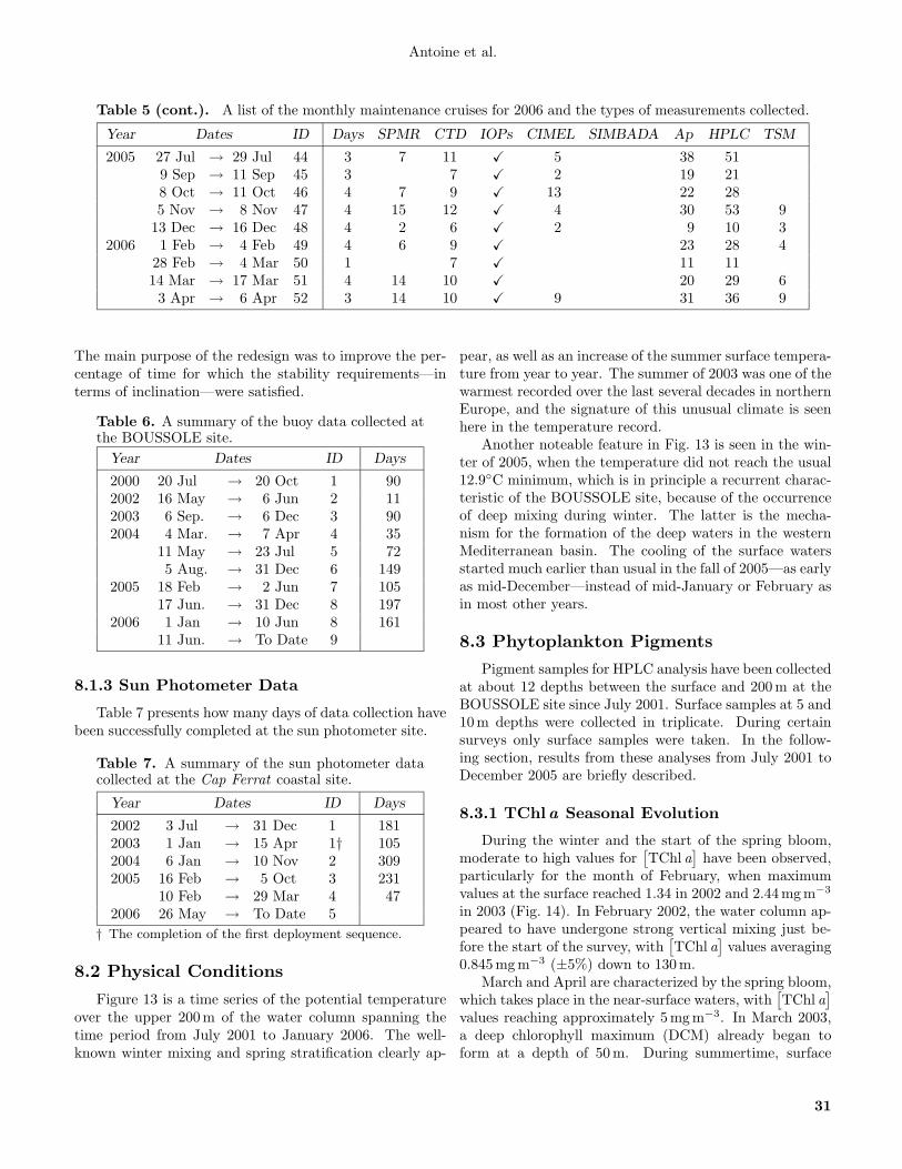
Antoine et al.
Table 5 (cont.). A list of the monthly maintenance cruises for 2006 and the types of measurements collected.
Year Dates ID Days SPMR CTD IOPs CIMEL SIMBADA Ap HPLC TSM
2005 27 Jul → 29 Jul 44 3 7 11 � 5 38 519 Sep → 11 Sep 45 3 7 � 2 19 218 Oct → 11 Oct 46 4 7 9 � 13 22 285 Nov → 8 Nov 47 4 15 12 � 4 30 53 9
13 Dec → 16 Dec 48 4 2 6 � 2 9 10 32006 1 Feb → 4 Feb 49 4 6 9 � 23 28 4
28 Feb → 4 Mar 50 1 7 � 11 1114 Mar → 17 Mar 51 4 14 10 � 20 29 63 Apr → 6 Apr 52 3 14 10 � 9 31 36 9
The main purpose of the redesign was to improve the per-centage of time for which the stability requirements—interms of inclination—were satisfied.
Table 6. A summary of the buoy data collected atthe BOUSSOLE site.
Year Dates ID Days
2000 20 Jul → 20 Oct 1 902002 16 May → 6 Jun 2 112003 6 Sep. → 6 Dec 3 902004 4 Mar. → 7 Apr 4 35
11 May → 23 Jul 5 725 Aug. → 31 Dec 6 149
2005 18 Feb → 2 Jun 7 10517 Jun. → 31 Dec 8 197
2006 1 Jan → 10 Jun 8 16111 Jun. → To Date 9
8.1.3 Sun Photometer Data
Table 7 presents how many days of data collection havebeen successfully completed at the sun photometer site.
Table 7. A summary of the sun photometer datacollected at the Cap Ferrat coastal site.
Year Dates ID Days
2002 3 Jul → 31 Dec 1 1812003 1 Jan → 15 Apr 1† 1052004 6 Jan → 10 Nov 2 3092005 16 Feb → 5 Oct 3 231
10 Feb → 29 Mar 4 472006 26 May → To Date 5
† The completion of the first deployment sequence.
8.2 Physical Conditions
Figure 13 is a time series of the potential temperatureover the upper 200 m of the water column spanning thetime period from July 2001 to January 2006. The well-known winter mixing and spring stratification clearly ap-
pear, as well as an increase of the summer surface tempera-ture from year to year. The summer of 2003 was one of thewarmest recorded over the last several decades in northernEurope, and the signature of this unusual climate is seenhere in the temperature record.
Another noteable feature in Fig. 13 is seen in the win-ter of 2005, when the temperature did not reach the usual12.9◦C minimum, which is in principle a recurrent charac-teristic of the BOUSSOLE site, because of the occurrenceof deep mixing during winter. The latter is the mecha-nism for the formation of the deep waters in the westernMediterranean basin. The cooling of the surface watersstarted much earlier than usual in the fall of 2005—as earlyas mid-December—instead of mid-January or February asin most other years.
8.3 Phytoplankton Pigments
Pigment samples for HPLC analysis have been collectedat about 12 depths between the surface and 200 m at theBOUSSOLE site since July 2001. Surface samples at 5 and10 m depths were collected in triplicate. During certainsurveys only surface samples were taken. In the follow-ing section, results from these analyses from July 2001 toDecember 2005 are briefly described.
8.3.1 TChla Seasonal Evolution
During the winter and the start of the spring bloom,moderate to high values for
[TChl a
]have been observed,
particularly for the month of February, when maximumvalues at the surface reached 1.34 in 2002 and 2.44 mg m−3
in 2003 (Fig. 14). In February 2002, the water column ap-peared to have undergone strong vertical mixing just be-fore the start of the survey, with
[TChl a
]values averaging
0.845 mg m−3 (±5%) down to 130 m.March and April are characterized by the spring bloom,
which takes place in the near-surface waters, with[TChl a
]values reaching approximately 5 mg m−3. In March 2003,a deep chlorophyll maximum (DCM) already began toform at a depth of 50 m. During summertime, surface
31
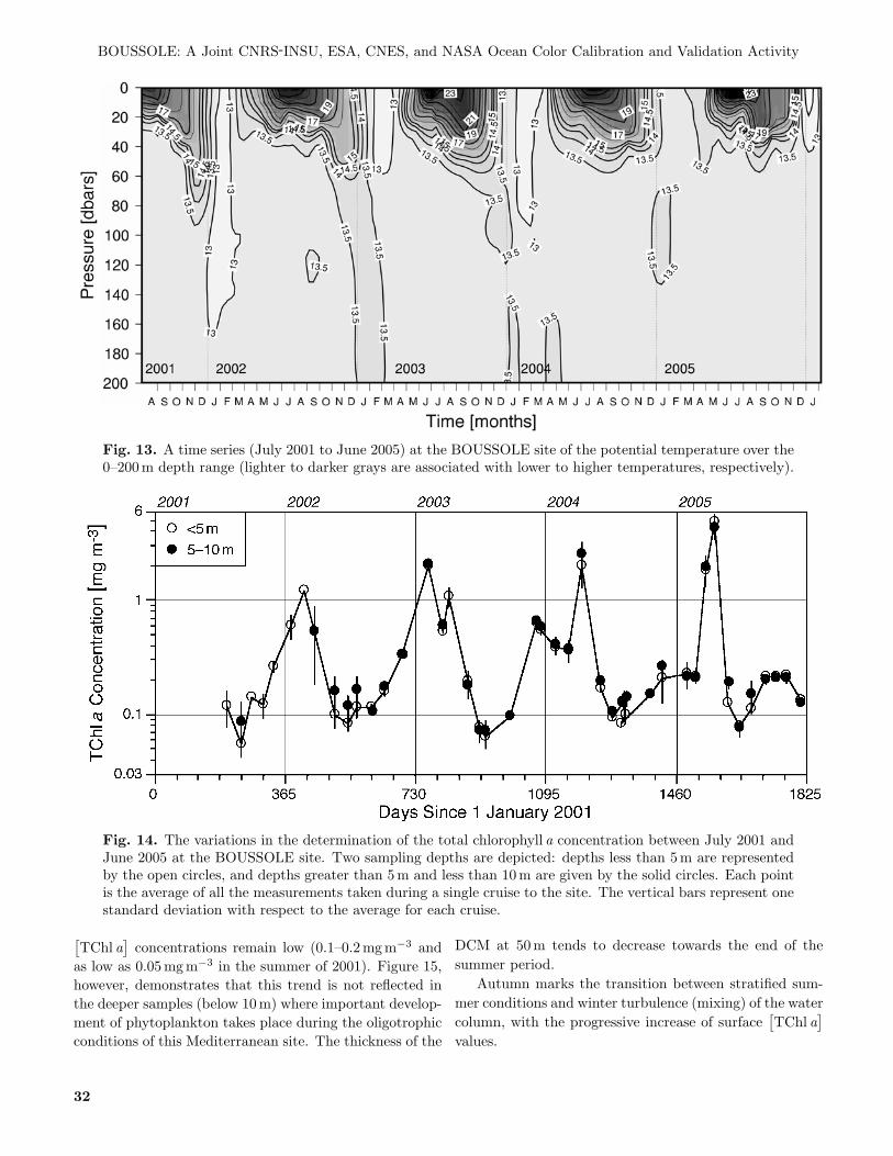
BOUSSOLE: A Joint CNRS-INSU, ESA, CNES, and NASA Ocean Color Calibration and Validation Activity
Fig. 13. A time series (July 2001 to June 2005) at the BOUSSOLE site of the potential temperature over the0–200 m depth range (lighter to darker grays are associated with lower to higher temperatures, respectively).
Fig. 14. The variations in the determination of the total chlorophyll a concentration between July 2001 andJune 2005 at the BOUSSOLE site. Two sampling depths are depicted: depths less than 5 m are representedby the open circles, and depths greater than 5 m and less than 10 m are given by the solid circles. Each pointis the average of all the measurements taken during a single cruise to the site. The vertical bars represent onestandard deviation with respect to the average for each cruise.
[TChl a
]concentrations remain low (0.1–0.2 mg m−3 and
as low as 0.05 mg m−3 in the summer of 2001). Figure 15,however, demonstrates that this trend is not reflected inthe deeper samples (below 10 m) where important develop-ment of phytoplankton takes place during the oligotrophicconditions of this Mediterranean site. The thickness of the
DCM at 50 m tends to decrease towards the end of thesummer period.
Autumn marks the transition between stratified sum-mer conditions and winter turbulence (mixing) of the watercolumn, with the progressive increase of surface
[TChl a
]values.
32
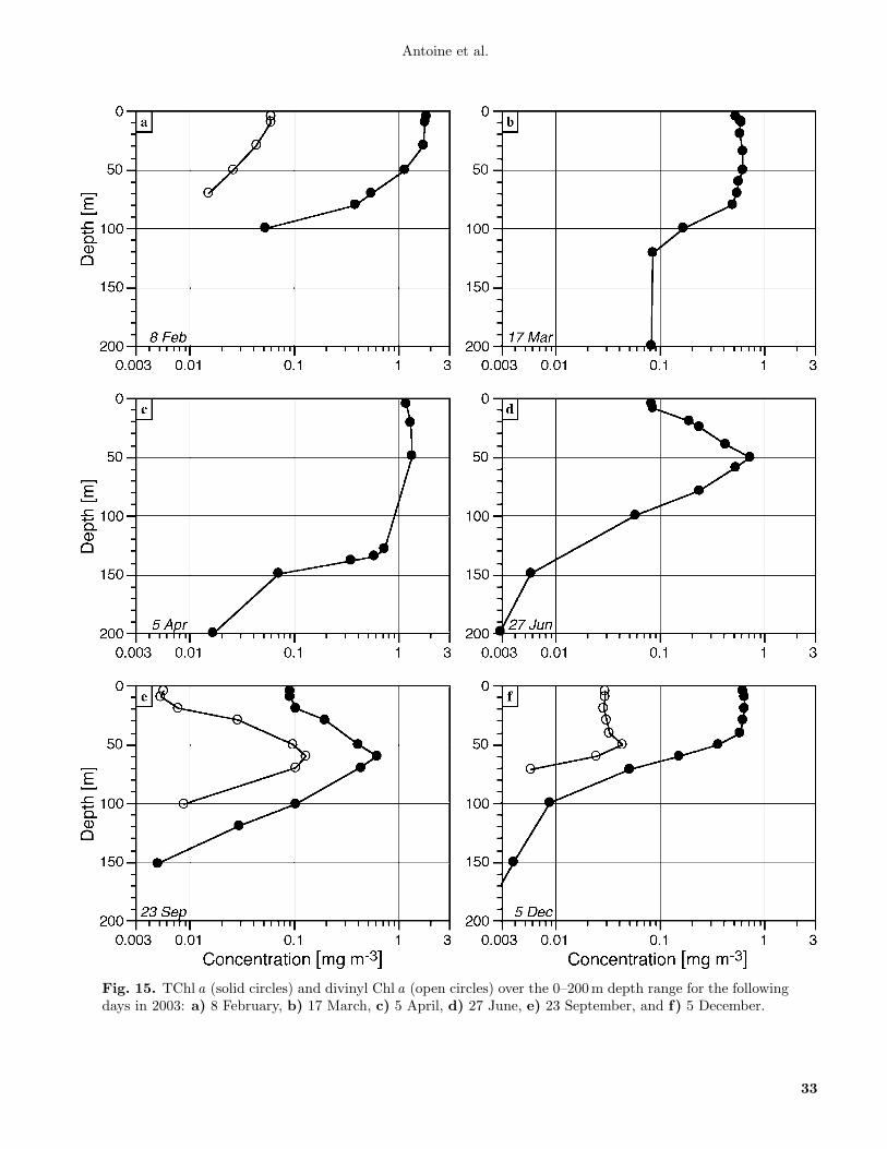
Antoine et al.
Fig. 15. TChl a (solid circles) and divinyl Chl a (open circles) over the 0–200 m depth range for the followingdays in 2003: a) 8 February, b) 17 March, c) 5 April, d) 27 June, e) 23 September, and f) 5 December.
33

BOUSSOLE: A Joint CNRS-INSU, ESA, CNES, and NASA Ocean Color Calibration and Validation Activity
Fig. 16. A time series of average abundances of pico- (circles), nano- (diamonds), and micro- (squares)phytoplankton for surface samples (less than 20 m) between July 2001 and October 2005. Each point is theaverage over all measurements taken during a cruise. The gray shading is arbitrarily assigned to enhancethe interpretation of the time series. The light and middle gray portions show the dominant separation ofthe community composition (in terms of contribution to the TChl a concentration) into a smaller percentageof microplankton and a larger percentage of nanoplankton, respectively. The exceptions are denoted bythe occasional reversals highlighted in the darkest gray. The seasonal contributions of the picoplankton areindicated by the bold line.
8.3.2 Changes in Community Structure
Six carotenoids and total chlorophyll b were used to par-tition the phytoplankton into three size classes based onthe unique aspects of the pigments used to establish theclassification scheme. The fractions of the Chl a concen-tration associated with each of the pico-, nano-, and micro-plankton classes (fp, fn, and fm, respectively) are derivedusing the following relationships (Uitz et al. 2006):
fp =0.86
[Zea
]+ 1.01
[TChl b
][DP
] , (10)
fn =1.27
[Hex
]+ 0.35
[But
]+ 0.6
[Allo
][DP
] , (11)
and
fm =1.41
[Fuco
]+ 1.41
[Peri
][DP
] , (12)
where the diagnostic pigment, DP, is simply the sum ofthe seven pigment concentrations used to distinguish thethree size classes.
Figure 16 presents the variations of these three classesfor near-surface (between 0–10 m) waters between the mid-dle of 2001 and the end of 2005. Generally, for surface wa-ters, microphytoplankton (characterized by diatoms and
dinoflagellates) and nanophytoplankton (characterized byprymnesiophytes and crysophytes) tend to vary in opposi-tion with picophytoplankton (characterized by cyanobac-teria at this site). The first are not a dominant class overthe studied period, with minimum values in autumn. Nev-ertheless, at depth, microphytoplankton can reach impor-tant proportions relative to the other two classes, partic-ularly in spring. Nanophytoplankton is a dominant classin surface waters over most of the year, except during theautumn when picophytoplankton tend to take over. TheDCM, however, is dominated by nanophytoplankton overthe whole summer–autumn time period.
The presence of divinyl Chl a, which is an indicator ofprochlorophytes, has generally been observed during au-tumn at the DCM and even in surface waters during winterconvection. In regards to the presence and concentrationsof Chl a degradation products (e.g., chlorophyllide a andphaeophorbide a), they are most often below the detectionlimits of the HPLC method.
8.4 AOPs from Ship OperationsFigure 17 panels a, b, and c show the July 2001 to Au-
gust 2004 time series of the reflectance ratio R(λ)/R(560),for λ=443, 490, and 510 nm, respectively. Figure 18 shows,for the same time period, the diffuse attenuation coeffi-cients of the upper layers for the wavelengths 412, 490,
34
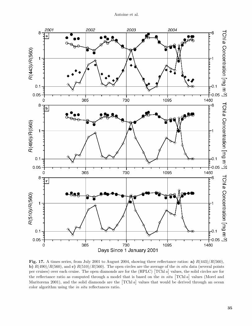
Antoine et al.
Fig. 17. A times series, from July 2001 to August 2004, showing three reflectance ratios: a) R(443)/R(560),b) R(490)/R(560), and c) R(510)/R(560). The open circles are the average of the in situ data (several pointsper cruises) over each cruise. The open diamonds are for the (HPLC)
[TChl a
]values, the solid circles are for
the reflectance ratio as computed through a model that is based on the in situ[TChl a
]values (Morel and
Maritorena 2001), and the solid diamonds are the[TChl a
]values that would be derived through an ocean
color algorithm using the in situ reflectances ratio.
35

BOUSSOLE: A Joint CNRS-INSU, ESA, CNES, and NASA Ocean Color Calibration and Validation Activity
Fig. 18. A times series, from July 2001 to August 2004, showing three diffuse attenuation coefficients: a)Kd(412), b) Kd(490), and c) Kd(560). The open circles are the average of the in situ data (several pointsper cruises) over each cruise. The open diamonds are for the (HPLC)
[TChl a
]values, and the solid circles
are for the Kd values as computed through a model that is based on the in situ[TChl a
]values (Morel and
Maritorena 2001).
36
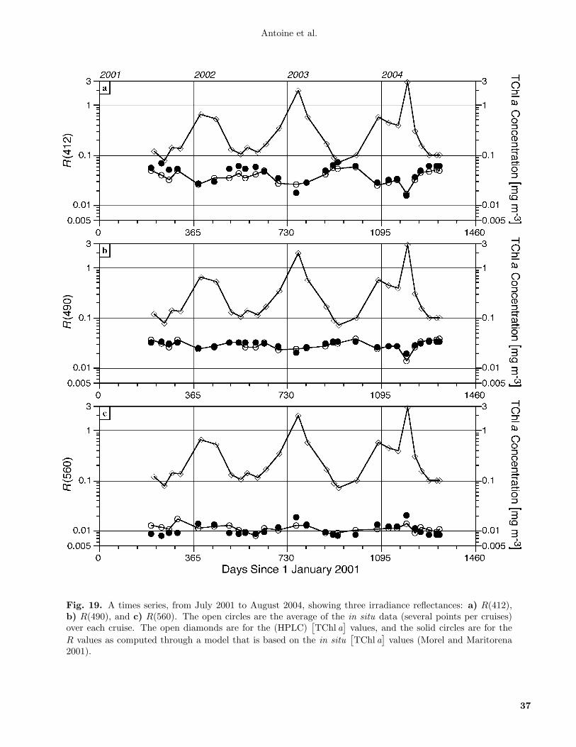
Antoine et al.
Fig. 19. A times series, from July 2001 to August 2004, showing three irradiance reflectances: a) R(412),b) R(490), and c) R(560). The open circles are the average of the in situ data (several points per cruises)over each cruise. The open diamonds are for the (HPLC)
[TChl a
]values, and the solid circles are for the
R values as computed through a model that is based on the in situ[TChl a
]values (Morel and Maritorena
2001).
37
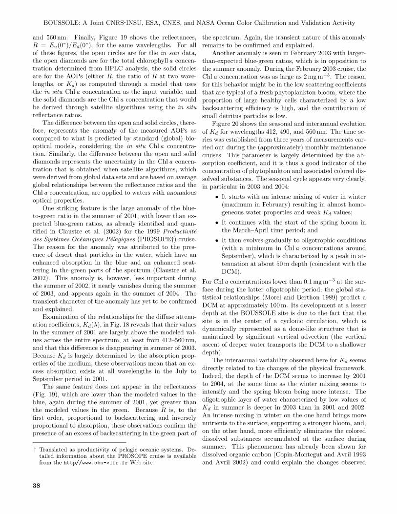
BOUSSOLE: A Joint CNRS-INSU, ESA, CNES, and NASA Ocean Color Calibration and Validation Activity
and 560 nm. Finally, Figure 19 shows the reflectances,R = Eu(0-)/Ed(0-), for the same wavelengths. For allof these figures, the open circles are for the in situ data,the open diamonds are for the total chlorophyll a concen-tration determined from HPLC analysis, the solid circlesare for the AOPs (either R, the ratio of R at two wave-lengths, or Kd) as computed through a model that usesthe in situ Chl a concentration as the input variable, andthe solid diamonds are the Chl a concentration that wouldbe derived through satellite algorithms using the in situreflectance ratios.
The difference between the open and solid circles, there-fore, represents the anomaly of the measured AOPs ascompared to what is predicted by standard (global) bio-optical models, considering the in situ Chl a concentra-tion. Similarly, the difference between the open and soliddiamonds represents the uncertainty in the Chl a concen-tration that is obtained when satellite algorithms, whichwere derived from global data sets and are based on averageglobal relationships between the reflectance ratios and theChl a concentration, are applied to waters with anomalousoptical properties.
One striking feature is the large anomaly of the blue-to-green ratio in the summer of 2001, with lower than ex-pected blue-green ratios, as already identified and quan-tified in Claustre et al. (2002) for the 1999 Productivitedes Systemes Oceaniques Pelagiques (PROSOPE†) cruise.The reason for the anomaly was attributed to the pres-ence of desert dust particles in the water, which have anenhanced absorption in the blue and an enhanced scat-tering in the green parts of the spectrum (Claustre et al.2002). This anomaly is, however, less important duringthe summer of 2002, it nearly vanishes during the summerof 2003, and appears again in the summer of 2004. Thetransient character of the anomaly has yet to be confirmedand explained.
Examination of the relationships for the diffuse attenu-ation coefficients, Kd(λ), in Fig. 18 reveals that their valuesin the summer of 2001 are largely above the modeled val-ues across the entire spectrum, at least from 412–560 nm,and that this difference is disappearing in summer of 2003.Because Kd is largely determined by the absorption prop-erties of the medium, these observations mean that an ex-cess absorption exists at all wavelengths in the July toSeptember period in 2001.
The same feature does not appear in the reflectances(Fig. 19), which are lower than the modeled values in theblue, again during the summer of 2001, yet greater thanthe modeled values in the green. Because R is, to thefirst order, proportional to backscattering and inverselyproportional to absorption, these observations confirm thepresence of an excess of backscattering in the green part of
† Translated as productivity of pelagic oceanic systems. De-tailed information about the PROSOPE cruise is availablefrom the http//www.obs-vlfr.fr Web site.
the spectrum. Again, the transient nature of this anomalyremains to be confirmed and explained.
Another anomaly is seen in February 2003 with larger-than-expected blue-green ratios, which is in opposition tothe summer anomaly. During the February 2003 cruise, theChl a concentration was as large as 2 mg m−3. The reasonfor this behavior might be in the low scattering coefficientsthat are typical of a fresh phytoplankton bloom, where theproportion of large healthy cells characterized by a lowbackscattering efficiency is high, and the contribution ofsmall detritus particles is low.
Figure 20 shows the seasonal and interannual evolutionof Kd for wavelengths 412, 490, and 560 nm. The time se-ries was established from three years of measurements car-ried out during the (approximately) monthly maintenancecruises. This parameter is largely determined by the ab-sorption coefficient, and it is thus a good indicator of theconcentration of phytoplankton and associated colored dis-solved substances. The seasonal cycle appears very clearly,in particular in 2003 and 2004:
• It starts with an intense mixing of water in winter(maximum in February) resulting in almost homo-geneous water properties and weak Kd values;
• It continues with the start of the spring bloom inthe March–April time period; and
• It then evolves gradually to oligotrophic conditions(with a minimum in Chl a concentrations aroundSeptember), which is characterized by a peak in at-tenuation at about 50 m depth (coincident with theDCM).
For Chl a concentrations lower than 0.1 mg m−3 at the sur-face during the latter oligotrophic period, the global sta-tistical relationships (Morel and Berthon 1989) predict aDCM at approximately 100 m. Its development at a lesserdepth at the BOUSSOLE site is due to the fact that thesite is in the center of a cyclonic circulation, which isdynamically represented as a dome-like structure that ismaintained by significant vertical advection (the verticalascent of deeper water transports the DCM to a shallowerdepth).
The interannual variability observed here for Kd seemsdirectly related to the changes of the physical framework.Indeed, the depth of the DCM seems to increase by 2001to 2004, at the same time as the winter mixing seems tointensify and the spring bloom being more intense. Theoligotrophic layer of water characterized by low values ofKd in summer is deeper in 2003 than in 2001 and 2002.An intense mixing in winter on the one hand brings morenutrients to the surface, supporting a stronger bloom, and,on the other hand, more efficiently eliminates the coloreddissolved substances accumulated at the surface duringsummer. This phenomenon has already been shown fordissolved organic carbon (Copin-Montegut and Avril 1993and Avril 2002) and could explain the changes observed
38
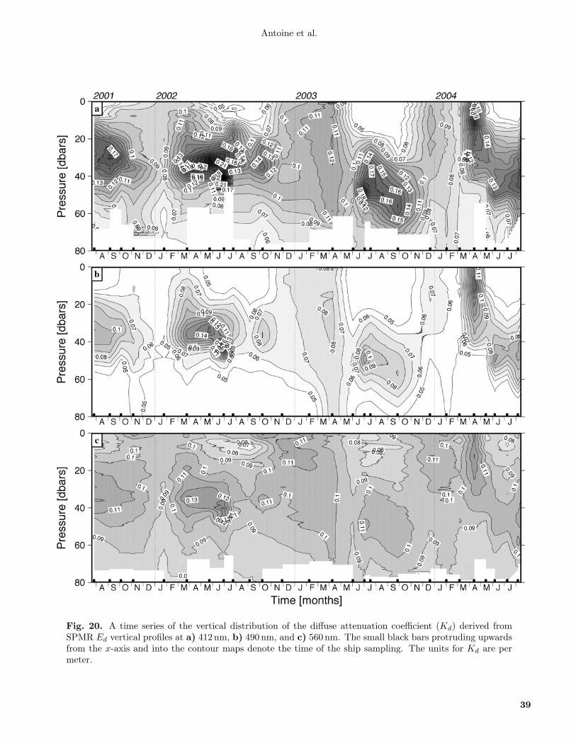
Antoine et al.
Fig. 20. A time series of the vertical distribution of the diffuse attenuation coefficient (Kd) derived fromSPMR Ed vertical profiles at a) 412 nm, b) 490 nm, and c) 560 nm. The small black bars protruding upwardsfrom the x-axis and into the contour maps denote the time of the ship sampling. The units for Kd are permeter.
39
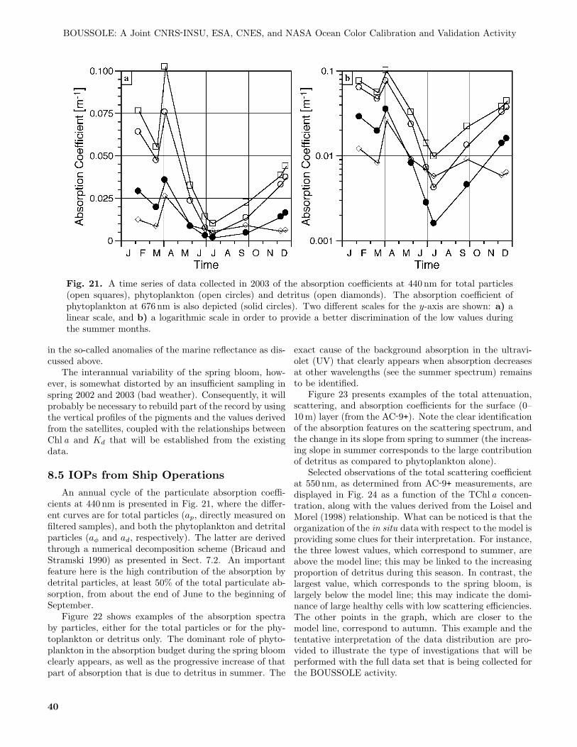
BOUSSOLE: A Joint CNRS-INSU, ESA, CNES, and NASA Ocean Color Calibration and Validation Activity
Fig. 21. A time series of data collected in 2003 of the absorption coefficients at 440 nm for total particles(open squares), phytoplankton (open circles) and detritus (open diamonds). The absorption coefficient ofphytoplankton at 676 nm is also depicted (solid circles). Two different scales for the y-axis are shown: a) alinear scale, and b) a logarithmic scale in order to provide a better discrimination of the low values duringthe summer months.
in the so-called anomalies of the marine reflectance as dis-cussed above.
The interannual variability of the spring bloom, how-ever, is somewhat distorted by an insufficient sampling inspring 2002 and 2003 (bad weather). Consequently, it willprobably be necessary to rebuild part of the record by usingthe vertical profiles of the pigments and the values derivedfrom the satellites, coupled with the relationships betweenChl a and Kd that will be established from the existingdata.
8.5 IOPs from Ship Operations
An annual cycle of the particulate absorption coeffi-cients at 440 nm is presented in Fig. 21, where the differ-ent curves are for total particles (ap, directly measured onfiltered samples), and both the phytoplankton and detritalparticles (aφ and ad, respectively). The latter are derivedthrough a numerical decomposition scheme (Bricaud andStramski 1990) as presented in Sect. 7.2. An importantfeature here is the high contribution of the absorption bydetrital particles, at least 50% of the total particulate ab-sorption, from about the end of June to the beginning ofSeptember.
Figure 22 shows examples of the absorption spectraby particles, either for the total particles or for the phy-toplankton or detritus only. The dominant role of phyto-plankton in the absorption budget during the spring bloomclearly appears, as well as the progressive increase of thatpart of absorption that is due to detritus in summer. The
exact cause of the background absorption in the ultravi-olet (UV) that clearly appears when absorption decreasesat other wavelengths (see the summer spectrum) remainsto be identified.
Figure 23 presents examples of the total attenuation,scattering, and absorption coefficients for the surface (0–10 m) layer (from the AC-9+). Note the clear identificationof the absorption features on the scattering spectrum, andthe change in its slope from spring to summer (the increas-ing slope in summer corresponds to the large contributionof detritus as compared to phytoplankton alone).
Selected observations of the total scattering coefficientat 550 nm, as determined from AC-9+ measurements, aredisplayed in Fig. 24 as a function of the TChl a concen-tration, along with the values derived from the Loisel andMorel (1998) relationship. What can be noticed is that theorganization of the in situ data with respect to the model isproviding some clues for their interpretation. For instance,the three lowest values, which correspond to summer, areabove the model line; this may be linked to the increasingproportion of detritus during this season. In contrast, thelargest value, which corresponds to the spring bloom, islargely below the model line; this may indicate the domi-nance of large healthy cells with low scattering efficiencies.The other points in the graph, which are closer to themodel line, correspond to autumn. This example and thetentative interpretation of the data distribution are pro-vided to illustrate the type of investigations that will beperformed with the full data set that is being collected forthe BOUSSOLE activity.
40
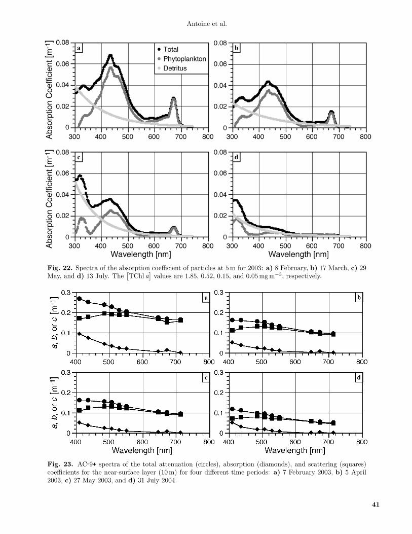
Antoine et al.
Fig. 22. Spectra of the absorption coefficient of particles at 5 m for 2003: a) 8 February, b) 17 March, c) 29May, and d) 13 July. The
[TChl a
]values are 1.85, 0.52, 0.15, and 0.05 mg m−3, respectively.
Fig. 23. AC-9+ spectra of the total attenuation (circles), absorption (diamonds), and scattering (squares)coefficients for the near-surface layer (10 m) for four different time periods: a) 7 February 2003, b) 5 April2003, c) 27 May 2003, and d) 31 July 2004.
41
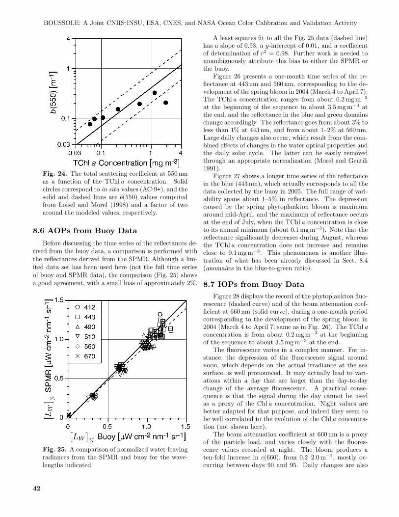
BOUSSOLE: A Joint CNRS-INSU, ESA, CNES, and NASA Ocean Color Calibration and Validation Activity
Fig. 24. The total scattering coefficient at 550 nmas a function of the TChl a concentration. Solidcircles correspond to in situ values (AC-9+), and thesolid and dashed lines are b(550) values computedfrom Loisel and Morel (1998) and a factor of twoaround the modeled values, respectively.
8.6 AOPs from Buoy Data
Before discussing the time series of the reflectances de-rived from the buoy data, a comparison is performed withthe reflectances derived from the SPMR. Although a lim-ited data set has been used here (not the full time seriesof buoy and SPMR data), the comparison (Fig. 25) showsa good agreement, with a small bias of approximately 2%.
Fig. 25. A comparison of normalized water-leavingradiances from the SPMR and buoy for the wave-lengths indicated.
A least squares fit to all the Fig. 25 data (dashed line)has a slope of 0.93, a y-intercept of 0.01, and a coefficientof determination of r2 = 0.98. Further work is needed tounambiguously attribute this bias to either the SPMR orthe buoy.
Figure 26 presents a one-month time series of the re-flectance at 443 nm and 560 nm, corresponding to the de-velopment of the spring bloom in 2004 (March 4 to April 7).The TChl a concentration ranges from about 0.2 mg m−3
at the beginning of the sequence to about 3.5 mg m−3 atthe end, and the reflectance in the blue and green domainschange accordingly. The reflectance goes from about 3% toless than 1% at 443 nm, and from about 1–2% at 560 nm.Large daily changes also occur, which result from the com-bined effects of changes in the water optical properties andthe daily solar cycle. The latter can be easily removedthrough an appropriate normalization (Morel and Gentili1991).
Figure 27 shows a longer time series of the reflectancein the blue (443 nm), which actually corresponds to all thedata collected by the buoy in 2005. The full range of vari-ability spans about 1–5% in reflectance. The depressioncaused by the spring phytoplankton bloom is maximumaround mid-April, and the maximum of reflectance occursat the end of July, when the TChl a concentration is closeto its annual minimum (about 0.1 mg m−3). Note that thereflectance significantly decreases during August, whereasthe TChl a concentration does not increase and remainsclose to 0.1 mg m−3. This phenomenon is another illus-tration of what has been already discussed in Sect. 8.4(anomalies in the blue-to-green ratio).
8.7 IOPs from Buoy DataFigure 28 displays the record of the phytoplankton fluo-
rescence (dashed curve) and of the beam attenuation coef-ficient at 660 nm (solid curve), during a one-month periodcorresponding to the development of the spring bloom in2004 (March 4 to April 7; same as in Fig. 26). The TChl aconcentration is from about 0.2 mg m−3 at the beginningof the sequence to about 3.5 mg m−3 at the end.
The fluorescence varies in a complex manner. For in-stance, the depression of the fluorescence signal aroundnoon, which depends on the actual irradiance at the seasurface, is well pronounced. It may actually lead to vari-ations within a day that are larger than the day-to-daychange of the average fluorescence. A practical conse-quence is that the signal during the day cannot be usedas a proxy of the Chl a concentration. Night values arebetter adapted for that purpose, and indeed they seem tobe well correlated to the evolution of the Chl a concentra-tion (not shown here).
The beam attenuation coefficient at 660 nm is a proxyof the particle load, and varies closely with the fluores-cence values recorded at night. The bloom produces aten-fold increase in c(660), from 0.2–2.0 m−1, mostly oc-curring between days 90 and 95. Daily changes are also
42
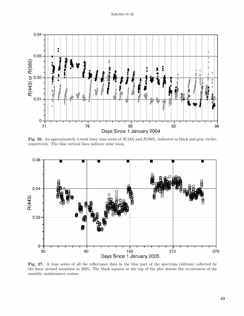
Antoine et al.
Fig. 26. An approximately 4-week buoy time series of R(443) and R(560), indicated as black and gray circles,respectively. The thin vertical lines indicate solar noon.
Fig. 27. A time series of all the reflectance data in the blue part of the spectrum (443 nm) collected bythe buoy around noontime in 2005. The black squares at the top of the plot denote the occurrences of themonthly maintenance cruises.
43

BOUSSOLE: A Joint CNRS-INSU, ESA, CNES, and NASA Ocean Color Calibration and Validation Activity
Fig. 28. An approximately 4-week buoy time series of the beam attenuation coefficient at 660 nm (blackcircles) and the phytoplankton fluorescence (gray circles). The latter is presented in relative units.
clearly shown, with a great variety of shapes, however, andsometimes with very fast increases (day 95 for instance) ordramatic declines (day 96). The maximum is usually oc-curring around noon or a few hours after noon. Inherentlyto Eulerian measurements at a fixed moored station, thesechanges are the result of the local phytoplankton growthand of lateral advection of water masses.
8.8 Sun Photometer Data
Figure 29 illustrates the overall data set that has beencollected up to now at the Cap Ferrat sun photometersite. What is shown is the aerosol optical thickness as de-rived by the AERONET project through their standardprocedures. The monthly AOT averages are usually min-imum in January or February, and several relative max-ima occur in spring (March or April), summer (usuallyJuly), and fall (October–November). The correspondingmonthly averages of the Angstrom exponent (not shown)are always above 1.0 m−1, which indicates the persistenceof small particles throughout the year.
The ability of the inversion method, which was devel-oped as part of the BOUSSOLE project and uses ground-based data to get aerosol optical properties (Sect. 7.7), isdemonstrated using days corresponding to MERIS over-passes. The results are presented in Fig. 30 for sequencesof principal planes corresponding to high solar zenith an-gles (typically above 70◦) to better cover the backscatter-ing region of measurements and to include the scatteringangle of 150◦. Table 8 presents the values of the retrieved
refractive index for these sequences. The agreement be-tween measurements and predictions is good, especially inthe backward direction for sky radiances. The degree ofpolarization is also accurately retrieved, especially at 90◦,which is of interest for classifying particle types.
These examples demonstrate it is possible to obtainsome information on the refractive indices of aerosols byusing the inversion method and, thus, to get the aerosolphase function. Such information can be used to predictthe angular distribution of the radiance and the degree ofpolarization, thus, it is likely that ground-based photome-ter measurements can be used for the vicarious calibrationof satellite ocean color sensors (Sect. 10).
9. SATELLITE VALIDATIONMatch-up analyses of the water-leaving radiances, as
well as for the Chl a concentrations, have been performedfor the MERIS, SeaWiFS, and MODIS-A data products.The analyses all follow the same procedure, wherein a 5×5pixel box is extracted from the level -2 product (see below),and directly compared to the same quantity as derivedfrom the in situ data (ship or buoy). For the SeaWiFS andMODIS-A sensors, the criteria used for a given comparisonpoint to be excluded in the final analysis are described byBailey et al. (2000). They are essentially the same forMERIS data, except the flags are not identical.
The combination of data availability, orbit character-istics, and the quality criteria used in match-up processyields 68 matchups for MERIS (data from September 2003to December 2005), 89 matchups for SeaWiFS (data from
44
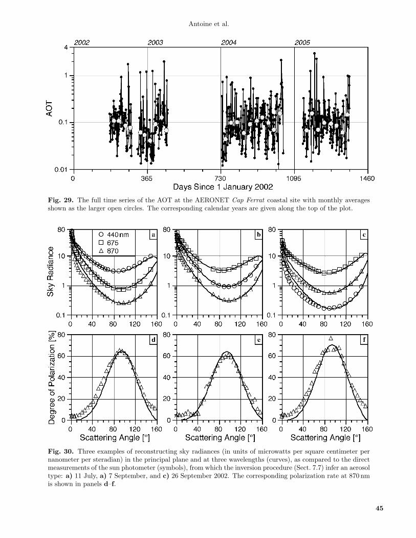
Antoine et al.
Fig. 29. The full time series of the AOT at the AERONET Cap Ferrat coastal site with monthly averagesshown as the larger open circles. The corresponding calendar years are given along the top of the plot.
Fig. 30. Three examples of reconstructing sky radiances (in units of microwatts per square centimeter pernanometer per steradian) in the principal plane and at three wavelengths (curves), as compared to the directmeasurements of the sun photometer (symbols), from which the inversion procedure (Sect. 7.7) infer an aerosoltype: a) 11 July, a) 7 September, and c) 26 September 2002. The corresponding polarization rate at 870 nmis shown in panels d–f.
45
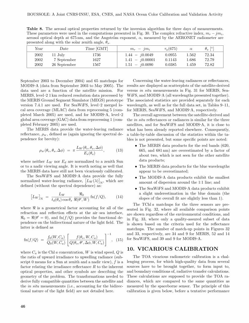
BOUSSOLE: A Joint CNRS-INSU, ESA, CNES, and NASA Ocean Color Calibration and Validation Activity
Table 8. The aerosol optical properties returned by the inversion algorithm for three days of measurements.These parameters were used in the computations presented in Fig. 30. The complex refractive index, mr − jmi,aerosol optical depth at 675 nm, and the Angstrom exponent, α, measured by the AERONET radiometer arepresented along with the solar zenith angle, θs.
Year Date Time [GMT] mr − jmi τa(675) α θs [◦]
2002 11 July 1736 1.44 − j0.0049 0.0955 1.562 72.342002 7 September 1627 1.41 − j0.00001 0.1143 1.686 72.792002 26 September 1567 1.51 − j0.0090 0.0385 1.459 72.82
September 2003 to December 2004) and 65 matchups forMODIS-A (data from September 2003 to May 2005). Thedata used are a function of the satellite mission. ForMERIS, level -2 1 km reduced resolution data processed bythe MERIS Ground Segment Simulator (MEGS) prototypeversion 7.4.1 are used. For SeaWiFS, level -2 merged lo-cal area coverage (MLAC) data from reprocessing 5 (com-pleted March 2005) are used, and for MODIS-A, level -2global area coverage (GAC) data from reprocessing 1 (com-pleted February 2005) are used.
The MERIS data provide the water-leaving radiancereflectance, ρW , defined as (again ignoring the spectral de-pendence for brevity):
ρW (θv, θs,∆φ) = πLW (θv, θs,∆φ)
Es(θs), (13)
where neither LW nor Ed are normalized to a zenith Sunor to a nadir viewing angle. It is worth noting as well thatthe MERIS data have still not been vicariously calibrated.
The SeaWiFS and MODIS-A data provide the fullynormalized water-leaving radiance,
[LW (λ)
]N, which are
defined (without the spectral dependence) as:
[LW
]N
=LW
td(θs) cos θs
�0
�(θ′, W )fn(f/Q), (14)
where � is a geometrical factor accounting for all of therefraction and reflection effects at the air–sea interface,�0 = �(θ′ = 0), and fn(f/Q) provides the functional de-pendence on the bidirectional nature of the light field. Thelatter is defined as
fn(f/Q) =f0(W, Ca)Q0(W, Ca)
[f(θs, W, Ca)
Q(θs, θ′,∆φ, W, Ca)
]−1
, (15)
where Ca is the Chl a concentration, W is wind speed, Q isthe ratio of upward irradiance to upwelling radiance (sub-script 0 means for a Sun at zenith and a nadir view), f is afactor relating the irradiance reflectance R to the inherentoptical properties, and other symbols are describing thegeometry of the problem. The transformations needed toderive fully compatible quantities between the satellite andthe in situ measurements (i.e., accounting for the bidirec-tional nature of the light field) are not detailed here.
Concerning the water-leaving radiances or reflectances,results are displayed as scatterplots of the satellite-derivedversus in situ measurements in Fig. 31 for MERIS, Sea-WiFS, and MODIS-A (all wavelengths presented together).The associated statistics are provided separately for eachwavelength, as well as for the full data set, in Tables 9–11,for MERIS, SeaWiFS, and MODIS-A, respectively.
The overall agreement between the satellite-derived andthe in situ reflectances or radiances is similar for the threesatellites, and for SeaWiFS and MODIS-A, it is close towhat has been already reported elsewhere. Consequently,a table-by-table discussion of the statistics within the ta-bles is not presented, but some specific points are noted:
• The MERIS data products for the red bands (620,665, and 681 nm) are overestimated by a factor ofabout two, which is not seen for the other satellitedata products;
• The MERIS data products for the blue wavelengthsappear to be overestimated;
• The MODIS-A data products exhibit the smallestamount of dispersion around the 1:1 line; and
• The SeaWiFS and MODIS-A data products exhibita slight underestimation in the blue domain (theslopes of the overall fit are slightly less than 1).
The TChl a matchups for the three sensors are pre-sented in Fig. 32, where all available comparison pointsare shown regardless of the environmental conditions, andin Fig. 33, where only a quality-assured subset of datais shown based on the criteria used for the reflectancematchups. The number of match-up points in Figures 32and 33, respectively, are 34 and 9 for MERIS, 52 and 14for SeaWiFS, and 39 and 9 for MODIS-A.
10. VICARIOUS CALIBRATIONThe TOA vicarious radiometric calibration is a chal-
lenging process, for which high-quality data from severalsources have to be brought together, to form input to,and boundary conditions of, radiative transfer calculations.These calculations are supposed to provide the TOA ra-diances, which are compared to the same quantities asmeasured by the spaceborne sensor. The principle of thiscalibration is given below, before a tentative performance
46
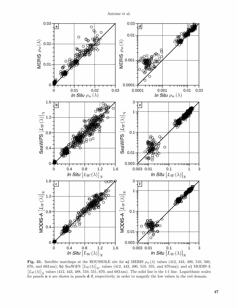
EE
E
E
E
E E
E
E
E
E E
E
E
E
E
E
E
E
EE
E
E
E
EE
E
E
E
EE
E
E
E
EE
E
E
E
E
EE
E
E
E
EE
E
E
EEE
E
E
E
EE
E
E
E
EE
E
E
E
EE
E
E
E
EE
E
E
E
EE
E
E
EE
E
E
E
E
E
E
EE
E
E
EE
E
E
EE
E
E
E
E
E
E
E
E
E
E
E
E
E
E
E
E
E
E
E
E
E
E
E
E
E
E
E
E
E
E
E
E
E
E
E
E
E
E
E
E
E
E
E
E
E
E
EE
E
E
EE
E
E
EE
E
E
EE
E
E
E
E
E
E
E
E
E
E
E
E
E
E
E
E
E
E
EE
E
E
EE
E
E
EE
E
E
E
EE
E
E
E
EE
E
E
E
EE
E
E
E
EE
E
E
E
E
EE
E
E
EEE
E
E
EE
E
E
E
EE
E
E
E
EEE
E
E
EE
E
E
E
E
EE
E
E
EE
E
E
E
EE
E
E
E
E
E
E
E
E
E
E
EE
E
E
EE
E
E
EE
E
E
EE
E
E
EE
E
E
EE
E
E
E
E
E
E
EE
E
E
E
E
E
E
E
E
E
E
E
E
E
E
EE
E
E
E
E
E
E
EE
E
E
E
EE
E
E
E
EE
E
E
EEE
E
E
E
EE
E
E
E
EE
E
E
EE
E
E
E
E
EEE
E
E
E
EEE
EE
E
EEEEE
E
EE
E
E
E
E
E
E
E
E
E
E
EE
E
E
E
E
E
EE
EE
E0
0.4
0.8
1.2
1.6
0 0.4 0.8 1.2 1.6
c
E
EE
E
E
E
EE
E
E
E
E
E E
E
E
E
E
EE
E
E
E
E
EE
E
E
E
E
EE
E
E
E
E
EE
E
E
E
E
E E
E
E
E
E
EE
E
E
E
E
EE
E
E
E
E
E
EE
E
E
E
E
EE
E
E
E
E
EE
E
E
E
E
EE
E
E
E
E
EE
E
E
E
E
EE
E
E
E
E
E
E
E
E
EE
E
E
E
EEE
E
E
EE
E
E
E
EE
E
E
E
EE
E
E
E
E
EE
E
E
EE
E
E
E
EE
E
E
E
E
E
E
E
E
E
E
E
E
E
E
E
E
E
E
E
E
E
E
E
E
E
E
E
E
E
E
E
E
E
E
E
E
E
E
EE
E
E
E
E
E
E
E
E
EE
E
E
E
EE
E
E
E
E
E
E
E
E
E
E
E
E
EE
E
E
E
EE
E
E
E
E
E
E
E
E
EE
E
E
E
E
E
E
E
E
E
E
E
E
E
E
E
E
E
E
E
E
E
E
E
E
E
E
E
E
E
E
E
E
E
E
E
E
E
E
E
E
E
E
E
EE
E
E
E
E
E
E
E
E
E
E
E
E
E
E
E
E
E
E
EE
E
E
E
E
E
E
E
E
E
E
E E
E
E
E
E
EE
E
E
E
E
EE
E
E
E
E
EE
E
E
E
E
E
EE
E
E
E
E
EE
E
E
E
E
EE
E
E
E
E E
E
E
E
E
E
EE
E
E
E
EE
E
E
E
E
EE
E
E
E
E
E
E
E
E
EE
E
E
E
EE
E
E
E
E
E
E
E
E
EE
E
E
E
E
E
E
E
E
E
E
E
E
E
E
E
E
E
E
E
E
E
E
E
EE
E
E
E
E
E
E
E
E
E
EE
E
E
E
E
EE
E
E
E
E
EE
E
E
E
E
EE
E
E
E
E
EE
E
E
E
E
EE
E
E
E
E
EE
E
E
E
E
E
E
E
E
EE
E
E
E
E
E
EE
E
E
E
EE
E
E
E
E
EE
E
E
E
E
EE
E
E
E
E
EEE
E
EE
EEEE
E
EE
E
E
E
E
EE
E
E
E
E
E
E
E
E
E
E
EE
E
E
E
E
EE
E
E
E
E0
0.4
0.8
1.2
1.6
0 0.4 0.8 1.2 1.6
b
a
EEE
E
EE
EEE
E
EE
EEE
E
EE
EE
E
E
EE
E
E
E
E
EE
E
E
E
E
EE
E
E
E
E
EE
E
E
E
E
EE
E
E
E
E
EE
E
E
E
E
EE
E
E
E
E
EE
E
E
E
E
EE
E
E
E
E
EE
E
E
E
E
EE
E
E
E
E
EE
E
E
E
E
EE
E
E
E
E
EE
E
E
E
E
E
EE
E
E
E
E
E
EE
E
E
E
E
E
EE
EE
E
E
E
EE
E
E
E
E
E
EE
E
E
E
E
EE
E
E
E
E
EE
E
E
E
E
EE
E
E
E
E
EE
E
E
E
E
EE
E
E
E
E
EE
EE
E
E
E
EE
E
E
E
E
E
EE
E
E
E
E
E
EE
EE
E
E
E
EE
E EE
E
E
EE
EEE
E
E
EE
EEE
E
E
EE
EEE
E
E
EE
E
E
E
E
E
EEEE
EEE
E
E
EEEE
E
E
E
E
E
EEEE
E
EEEE
EEEE
E
E
E
E
E
EEEE
EE
E
E
E
EEE
EE
E
E
E
EEEE0
0.01
0.02
0.03
0 0.01 0.02 0.03
EEE
E
EE
EEE
E
EE
EEEE
EE
EEE
E
E
E
EE
E
E
E
EE
E
E
EE
EE
E
E
EE
EE
E
E
EE
EE
E
E
EE
EEE
E
EE
EE
E
E
EE
EE
E
E
EE
EE
E
E
EE
EE
E
E
EE
EEE
E
EE
EE
E
E
E
E
EE
E
E
EE
EEE
E
E
EE
EEE
E
E
E
E
EEE
E
E
EE
EEE
E
E
EE
EEE
E
E
EE
EE
E
E
E
E
EE
E
E
EE
EE
E
E
EE
EE
E
E
EE
EE
E
E
EE
EEE
E
EE
EEE
E
E
EE
EEE
E
E
EE
EEE
E
E
EE
EEEE
E
EE
EEEE
E
EE
EEEE
E
EE
EEEE
E
EE
EEEE
E
EE
EEE
E
E
E
EE
E
EEEE
E
E
EE
E
EEE
E
E
EEE
E
EEEEE
E
EE
E
EEE
E
E
E
EE
E
EEE
E
E
E
EE
EEE
E
E
E
EEE
0.0001
0.001
0.01
0.03
0.0001 0.001 0.01 0.03
d
EEEE
E
E
EEEE
E
E
EEE
E
E
E
EEE
E
E
E
EEE
E
E
E
EEE
E
E
E
EEE
E
E
E
EEE
E
E
E
EEE
E
E
E
EEEE
E
E
EEE
E
E
E
EEEE
E
E
EEE
E
E
E
EEE
E
E
E
EEE
E
E
E
EEEE
E
E
EEE
E
E
EEE
E
E
EEEE
E
EEEE
E
EEE
E
E
EEE
E
E
EEE
E
E
EEE
E
E
EEE
E
E
EEE
E
E
EEE
E
E
EEE
E
E
EEE
E
E
EEE
E
E
EEE
E
E
EEE
E
E
EEE
E
E
EEE
E
E
EEE
E
E
EEE
E
EEE
E
E
EEE
E
E
EEE
E
E
EEE
E
E
EEE
E
E
EEE
E
E
EEE
E
E
EEE
E
E
EEE
E
E
EEE
E
E
EEE
E
E
EEE
E
E
EEE
E
E
EEE
E
E
EEE
E
E
EEE
E
E
EEE
E
E
EEE
E
E
EEEE
E
E
EEEE
E
E
EEE
E
E
E
EEEE
E
E
EEEE
E
E
EEEE
E
E
EEE
E
E
E
EEEE
E
E
EEEE
E
E
EEEE
E
E
EEEE
E
E
EEEE
E
E
EEE
E
E
EEE
E
E
EEE
E
E
EEE
E
E
EEE
E
E
EEE
E
E
EEE
E
E
EEE
E
E
EEE
E
E
EEE
E
E
EEE
E
E
EEE
E
E
EEE
E
E
E
EEEE
E
E
EEE
E
E
E
EEE
E
E
E
EEE
E
E
E
EEEE
E
E
EEE
E
E
E
EEE
E
E
EEEE
E
E
EEEE
E
E
EEE
E
E
E
EEE
E
E
E
EEE
E
E
E
EEEE
EEEEEE
E
EEEE
E
E
EEEE
E
E
EEEE
E
E
EEEE
E
E
EEEE
E
E
0.003
0.01
0.1
1
3
0.003 0.01 0.1 1 3
e
EEE
E
E
EEE
E
E
EEE
E
EEE
E
E
EEE
E
E
EEE
E
E
EEE
E
E
EEE
E
E
EEE
E
E
EEE
E
E
EEE
E
E
EEE
E
E
EEE
E
E
EEE
E
E
EEE
E
E
EEE
E
E
EE
E
E
EE
E
E
EE
E
E
EE
E
E
EE
E
E
EE
E
E
EE
E
E
EE
E
E
EE
E
E
EE
E
E
EE
E
E
EE
E
E
EE
E
E
EE
E
E
EE
E
E
EE
E
E
EE
E
E
EE
E
E
EE
E
E
EE
E
E
EE
E
E
EE
E
E
EE
E
E
EE
E
E
EE
E
E
EE
E
E
EEE
E
E
EEE
E
E
EEE
E
E
EEE
E
E
EEE
E
E
EEE
E
E
EEE
E
E
EEE
E
E
EEE
E
E
EEE
E
E
EEE
E
E
EEE
E
E
EEE
E
E
EE
E
E
EE
E
E
EE
E
E
EE
E
E
EE
E
E
EE
E
E
EE
E
E
EE
E
E
EE
E
E
EE
E
E
EE
E
E
EE
E
E
EE
E
E
EE
E
E
EE
E
E
EE
E
E
EE
E
E
EEE
E
E
EEE
E
E
EEE
E
E
EEE
E
E
EEE
E
E
EEE
EE
E
EEE
EE
E
EEE
EE
E
EEEEE
E
EEE
EE
E
EEE
EE
E
EEE
EE
E
EEE
EE
E
0.003
0.01
0.1
1
3
0.003 0.01 0.1 1 3
f
Antoine et al.
Fig. 31. Satellite matchups at the BOUSSOLE site for a) MERIS ρW (λ) values (412, 443, 490, 510, 560,670, and 683 nm); b) SeaWiFS
[LW (λ)
]N, values (412, 443, 490, 510, 555, and 670 nm); and c) MODIS-A[
LW (λ)]N
values (412, 443, 488, 510, 551, 670, and 683 nm). The solid line is the 1:1 line. Logarithmic scalesfor panels a–c are shown in panels d–f, respectively, in order to magnify the low values in the red domain.
47
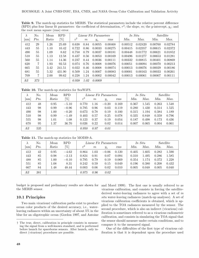
BOUSSOLE: A Joint CNRS-INSU, ESA, CNES, and NASA Ocean Color Calibration and Validation Activity
Table 9. The match-up statistics for MERIS. The statistical parameters include the relative percent difference(RPD) plus four linear fit parameters: the coefficient of determination, r2; the slope, m; the y-intercept, y0 ; andthe root mean square (rms) error.
λ No. Mean RPD Linear Fit Parameters In Situ Satellite[nm] Pts. Ratio [%] r2 m y0 rms Min. Max. Min. Max.
412 29 1.26 25.69 0.638 0.84 0.0055 0.00468 0.00512 0.02420 0.00760 0.02784443 55 1.10 10.42 0.722 0.86 0.0033 0.00275 0.00415 0.02357 0.00615 0.02372490 55 1.09 8.62 0.750 0.79 0.0037 0.00181 0.00448 0.01772 0.00621 0.01852510 55 1.13 12.58 0.437 0.56 0.0053 0.00169 0.00496 0.01277 0.00653 0.01281560 55 1.14 14.36 0.237 0.44 0.0036 0.00111 0.00332 0.00815 0.00401 0.00869620 7 1.93 92.53 0.074 0.76 0.0008 0.00076 0.00051 0.00094 0.00070 0.00213665 55 3.42 241.51 0.022 0.46 0.0008 0.00074 0.00013 0.00076 0.00029 0.00186681 55 5.32 431.90 0.509 1.24 0.0007 0.00083 0.00001 0.00163 0.00033 0.00261709 7 2.00 99.62 0.228 1.24 0.0002 0.00042 0.00013 0.00061 0.00007 0.00111
All 373 0.938 1.02 0.0009
Table 10. The match-up statistics for SeaWiFS.
λ No. Mean RPD Linear Fit Parameters In Situ Satellite[nm] Pts. Ratio [%] r2 m y0 rms Min. Max. Min. Max.
412 48 0.95 −5.10 0.770 1.16 −0.20 0.169 0.367 1.545 0.263 1.548443 98 0.99 −0.96 0.795 0.96 0.03 0.119 0.280 1.430 0.314 1.525490 98 1.00 −0.20 0.673 0.78 0.19 0.100 0.315 1.194 0.384 1.189510 98 0.99 −1.49 0.403 0.57 0.25 0.078 0.335 0.848 0.359 0.796555 98 1.01 1.08 0.123 0.37 0.19 0.054 0.187 0.498 0.173 0.436670 95 1.37 36.70 0.026 0.22 0.02 0.014 0.007 0.065 0.004 0.061
All 535 0.950 0.97 0.01
Table 11. The match-up statistics for MODIS-A.
λ No. Mean RPD Linear Fit Parameters In Situ Satellite[nm] Pts. Ratio [%] r2 m y0 rms Min. Max. Min. Max.
412 42 0.95 −4.62 0.864 1.03 −0.06 0.120 0.405 1.605 0.282 1.590443 85 0.98 −2.13 0.824 0.91 0.07 0.094 0.310 1.495 0.286 1.585488 85 1.00 −0.10 0.795 0.79 0.19 0.069 0.354 1.174 0.372 1.228551 85 1.08 8.31 0.242 0.59 0.15 0.049 0.196 0.380 0.208 0.432667 84 1.48 48.44 0.003 0.06 0.02 0.010 0.005 0.048 0.005 0.040
All 381 0.975 0.96 0.02
budget is proposed and preliminary results are shown forthe MERIS sensor.
10.1 PrinciplesTwo main vicarious† calibration paths exist to produce
ocean color products of the desired accuracy, i.e., water-leaving radiances within an uncertainty of about 5% in theblue for an oligotrophic ocean (Gordon 1997, and Antoine
† The true, direct, calibration in principle consists in measur-ing the signal from a well-known standard, and is performedbefore launch for spaceborne sensors. After launch, only in-direct (vicarious) procedures are possible.
and Morel 1999). The first one is usually referred to asvicarious calibration, and consists in forcing the satellite-derived water-leaving radiances to agree with a set of insitu water-leaving radiances (match-up analyses). A set ofvicarious calibration coefficients is obtained, which is ap-plied to the TOA radiances measured by the sensor. Thesecond procedure, which is also an indirect (vicarious) cal-ibration is sometimes referred to as a vicarious radiometriccalibration, and consists in simulating the TOA signal thatthe sensor should measure under certain conditions, and tocompare it to the measured signal.
One of the difficulties of the first type of vicarious cal-ibration is that it is dependent upon the procedure used
48

Antoine et al.
Fig. 32. In situ (HPLC) TChl a concentration matchups with respect to satellite-derived values at theBOUSSOLE site for a) MERIS (N = 34), b) SeaWiFS (N = 52), and c) MODIS-A (N = 39). The temporalcoverage is from July 2001 to the end of 2005 for MERIS and MODIS-A, and 2004 for SeaWiFS.
Fig. 33. The quality-assured in situ (HPLC) TChl a concentration matchups shown in Fig. 32 for a) MERIS(N = 9), b) SeaWiFS (N = 14), and c) MODIS-A (N = 9).
for the atmospheric correction of the TOA observations.Even if it is admittedly less dependent upon the selectedset of in situ water-leaving radiances, these measurementsalso contribute to the final accuracy. Besides the fact thatatmospheric measurements are not needed, the advantageof this technique is that the marine signals delivered byseveral sensors using different atmospheric correction al-gorithms can be cross-calibrated† provided the same setof in situ water-leaving radiances is used to perform thevicarious calibration (presently true for the SeaWiFS andMODIS-A sensors).
An inconvenience of the vicarious radiometric calibra-tion is that it requires a set of in situ measurements whichare usually difficult to collect, among other things, because
† Except in situations where the atmosphere would be signifi-cantly different from the atmosphere present when perform-ing the in situ measurements used for the vicarious calibra-tion exercise.
a high accuracy is required. In addition to the in-watermeasurements of the water-leaving radiances, this data setincludes sea state and atmospheric pressure, ozone concen-tration, aerosol optical thickness, aerosol type, and evenaerosol vertical profile if the aerosols reveal to be absorb-ing. If this data set is successfully assembled, the ad-vantage of the vicarious radiometric calibration is that itis independent of the atmospheric correction algorithms,so that the TOA signals of various sensors can be cross-calibrated. Then it is up to any user to apply its preferredatmospheric correction to these TOA signals. The marinesignals in that case might be inconsistent if significant dif-ferences exist in the various atmospheric corrections.
The greatest difficulty of the vicarious radiometric cal-ibration lies in the estimation of the aerosol optical thick-ness, phase function, and single scattering albedo. Theseparameters are accessible through the inversion of sun pho-tometer measurements, yet uncertainties inevitably occur
49
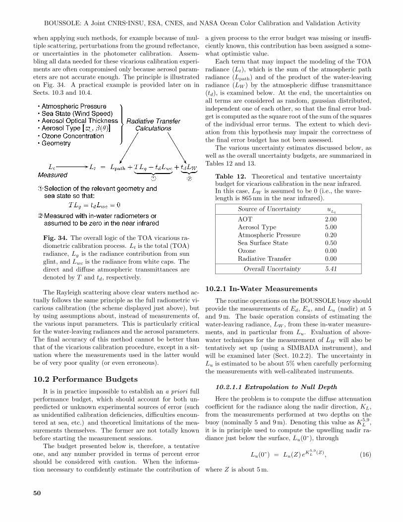
BOUSSOLE: A Joint CNRS-INSU, ESA, CNES, and NASA Ocean Color Calibration and Validation Activity
when applying such methods, for example because of mul-tiple scattering, perturbations from the ground reflectance,or uncertainties in the photometer calibration. Assem-bling all data needed for these vicarious calibration experi-ments are often compromised only because aerosol param-eters are not accurate enough. The principle is illustratedon Fig. 34. A practical example is provided later on inSects. 10.3 and 10.4.
Fig. 34. The overall logic of the TOA vicarious ra-diometric calibration process. Lt is the total (TOA)radiance, Lg is the radiance contribution from sunglint, and Lwc is the radiance from white caps. Thedirect and diffuse atmospheric transmittances aredenoted by T and td, respectively.
The Rayleigh scattering above clear waters method ac-tually follows the same principle as the full radiometric vi-carious calibration (the scheme displayed just above), butby using assumptions about, instead of measurements of,the various input parameters. This is particularly criticalfor the water-leaving radiances and the aerosol parameters.The final accuracy of this method cannot be better thanthat of the vicarious calibration procedure, except in a sit-uation where the measurements used in the latter wouldbe of very poor quality (or even erroneous).
10.2 Performance BudgetsIt is in practice impossible to establish an a priori full
performance budget, which should account for both un-predicted or unknown experimental sources of error (suchas unidentified calibration deficiencies, difficulties encoun-tered at sea, etc.) and theoretical limitations of the mea-surements themselves. The former are not totally knownbefore starting the measurement sessions.
The budget presented below is, therefore, a tentativeone, and any number provided in terms of percent errorshould be considered with caution. When the informa-tion necessary to confidently estimate the contribution of
a given process to the error budget was missing or insuffi-ciently known, this contribution has been assigned a some-what optimistic value.
Each term that may impact the modeling of the TOAradiance (Lt), which is the sum of the atmospheric pathradiance (Lpath) and of the product of the water-leavingradiance (LW ) by the atmospheric diffuse transmittance(td), is examined below. At the end, the uncertainties onall terms are considered as random, gaussian distributed,independent one of each other, so that the final error bud-get is computed as the square root of the sum of the squaresof the individual error terms. The extent to which devi-ation from this hypothesis may impair the correctness ofthe final error budget has not been assessed.
The various uncertainty estimates discussed below, aswell as the overall uncertainty budgets, are summarized inTables 12 and 13.
Table 12. Theoretical and tentative uncertaintybudget for vicarious calibration in the near infrared.In this case, LW is assumed to be 0 (i.e., the wave-length is 865 nm in the near infrared).
Source of Uncertainty uLt
AOT 2.00Aerosol Type 5.00Atmospheric Pressure 0.20Sea Surface State 0.50Ozone 0.00Radiative Transfer 0.00
Overall Uncertainty 5.41
10.2.1 In-Water Measurements
The routine operations on the BOUSSOLE buoy shouldprovide the measurements of Ed, Eu, and Lu (nadir) at 5and 9 m. The basic operation consists of estimating thewater-leaving radiance, LW , from these in-water measure-ments, and in particular from Lu. Evaluation of above-water techniques for the measurement of LW will also betentatively set up (using a SIMBADA instrument), andwill be examined later (Sect. 10.2.2). The uncertainty inLu is estimated to be about 5% when carefully performingthe measurements with well-calibrated instruments.
10.2.1.1 Extrapolation to Null Depth
Here the problem is to compute the diffuse attenuationcoefficient for the radiance along the nadir direction, KL,from the measurements performed at two depths on thebuoy (nominally 5 and 9 m). Denoting this value as K5,9
L ,it is in principle used to compute the upwelling nadir ra-diance just below the surface, Lu(0-), through
Lu(0-) = Lu(Z) eK5,9L
(Z), (16)
where Z is about 5 m.
50
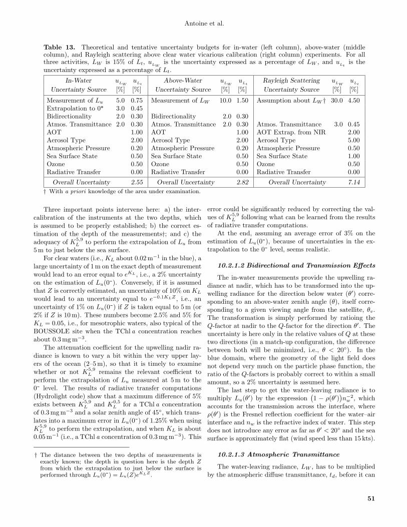
Antoine et al.
Table 13. Theoretical and tentative uncertainty budgets for in-water (left column), above-water (middlecolumn), and Rayleigh scattering above clear water vicarious calibration (right column) experiments. For allthree activities, LW is 15% of Lt, u
LWis the uncertainty expressed as a percentage of LW , and u
Ltis the
uncertainty expressed as a percentage of Lt.
In-Water uLW
uLt
Above-Water uLW
uLt
Rayleigh Scattering uLW
uLt
Uncertainty Source [%] [%] Uncertainty Source [%] [%] Uncertainty Source [%] [%]
Measurement of Lu 5.0 0.75 Measurement of LW 10.0 1.50 Assumption about LW † 30.0 4.50Extrapolation to 0+ 3.0 0.45Bidirectionality 2.0 0.30 Bidirectionality 2.0 0.30Atmos. Transmittance 2.0 0.30 Atmos. Transmittance 2.0 0.30 Atmos. Transmittance 3.0 0.45AOT 1.00 AOT 1.00 AOT Extrap. from NIR 2.00Aerosol Type 2.00 Aerosol Type 2.00 Aerosol Type 5.00Atmospheric Pressure 0.20 Atmospheric Pressure 0.20 Atmospheric Pressure 0.50Sea Surface State 0.50 Sea Surface State 0.50 Sea Surface State 1.00Ozone 0.50 Ozone 0.50 Ozone 0.50Radiative Transfer 0.00 Radiative Transfer 0.00 Radiative Transfer 0.00
Overall Uncertainty 2.55 Overall Uncertainty 2.82 Overall Uncertainty 7.14
† With a priori knowledge of the area under examination.
Three important points intervene here: a) the inter-calibration of the instruments at the two depths, whichis assumed to be properly established; b) the correct es-timation of the depth of the measurements†; and c) theadequacy of K5,9
L to perform the extrapolation of Lu from5 m to just below the sea surface.
For clear waters (i.e., KL about 0.02 m−1 in the blue), alarge uncertainty of 1 m on the exact depth of measurementwould lead to an error equal to eKL , i.e., a 2% uncertaintyon the estimation of Lu(0-). Conversely, if it is assumedthat Z is correctly estimated, an uncertainty of 10% on KL
would lead to an uncertainty equal to e−0.1KLZ , i.e., anuncertainty of 1% on Lu(0-) if Z is taken equal to 5 m (or2% if Z is 10 m). These numbers become 2.5% and 5% forKL = 0.05, i.e., for mesotrophic waters, also typical of theBOUSSOLE site when the TChl a concentration reachesabout 0.3 mg m−3.
The attenuation coefficient for the upwelling nadir ra-diance is known to vary a bit within the very upper lay-ers of the ocean (2–5 m), so that it is timely to examinewhether or not K5,9
L remains the relevant coefficient toperform the extrapolation of Lu measured at 5 m to the0- level. The results of radiative transfer computations(Hydrolight code) show that a maximum difference of 5%exists between K5,9
L and K0,5L for a TChl a concentration
of 0.3 mg m−3 and a solar zenith angle of 45◦, which trans-lates into a maximum error in Lu(0-) of 1.25% when usingK5,9
L to perform the extrapolation, and when KL is about0.05 m−1 (i.e., a TChl a concentration of 0.3 mg m−3). This
† The distance between the two depths of measurements isexactly known; the depth in question here is the depth Zfrom which the extrapolation to just below the surface isperformed through Lu(0-) = Lu(Z)eKLZ .
error could be significantly reduced by correcting the val-ues of K5,9
L following what can be learned from the resultsof radiative transfer computations.
At the end, assuming an average error of 3% on theestimation of Lu(0-), because of uncertainties in the ex-trapolation to the 0- level, seems realistic.
10.2.1.2 Bidirectional and Transmission Effects
The in-water measurements provide the upwelling ra-diance at nadir, which has to be transformed into the up-welling radiance for the direction below water (θ′) corre-sponding to an above-water zenith angle (θ), itself corre-sponding to a given viewing angle from the satellite, θv.The transformation is simply performed by ratioing theQ-factor at nadir to the Q-factor for the direction θ′. Theuncertainty is here only in the relative values of Q at thesetwo directions (in a match-up configuration, the differencebetween both will be minimized, i.e., θ < 20◦). In theblue domain, where the geometry of the light field doesnot depend very much on the particle phase function, theratio of the Q-factors is probably correct to within a smallamount, so a 2% uncertainty is assumed here.
The last step to get the water-leaving radiance is tomultiply Lu(θ′) by the expression
(1 − ρ(θ′)
)n−2
w , whichaccounts for the transmission across the interface, whereρ(θ′) is the Fresnel reflection coefficient for the water–airinterface and nw is the refractive index of water. This stepdoes not introduce any error as far as θ′ < 20◦ and the seasurface is approximately flat (wind speed less than 15 kts).
10.2.1.3 Atmospheric Transmittance
The water-leaving radiance, LW , has to be multipliedby the atmospheric diffuse transmittance, td, before it can
51
BOUSSOLE: A Joint CNRS-INSU, ESA, CNES, and NASA Ocean Color Calibration and Validation Activity
be added to the atmospheric path radiance. If the ex-pression in use for computing td is considered valid (Wang1999), the largest source of uncertainty is the aerosol op-tical thickness, which has a small impact on td. A factorof two change in τa (from 0.1 to 0.2), for example, trans-lates as a 2% error on td at 443 nm, which results in a 2%uncertainty on the product tdLW .
In the green domain (e.g., at approximately 550 nm),another source of uncertainty is the ozone content of theatmosphere. When λ = 550 nm, the Rayleigh optical thick-ness is about 0.09 and the ozone optical thickness is ap-proximately 0.03 for an ozone content of 350 DU. The un-certainty in td(550) corresponding to an uncertainty of50 DU would be of the order of 0.5% for viewing anglesless than 45◦ (with, for instance, td = e−(0.5τr+τoz)/ cos θv ).
10.2.2 Above-Water Measurements
The uncertainty to which LW is derived from the radi-ance measured above the sea surface (which includes LW
and surface reflection effects), can be considered as be-ing on the order of about 10% (Hooker et al. 2002b andHooker and Morel 2003), even when performed in well-controlled experimental conditions and in excellent envi-ronmental conditions. A careful implementation of the re-quired metrology and proper removal of glint effects duringdata processing can reduce the uncertainties to the sameorder as the calibration uncertainty (Hooker et al. 2004)for above- or in-water radiometers.
Because above-water measurements are collected wellabove the sea surface, the uncertainty attached to the ex-trapolation of in-water measurements from depth to justbeneath the surface does not enter into account. Thesame uncertainty is attached to the determination of bi-directional effects (Q factors), as well as to the calculationof the atmospheric diffuse transmittance.
10.2.3 Atmospheric Path Radiance
The uncertainties assoicated with computing the at-mospheric path radiance are examined based on the un-certainties in the parameters used in the computations.
10.2.3.1 Atmospheric Pressure
Atmospheric pressure, P , is known to within 0.5% (i.e.,5 hPa). The changes in the path reflectance due to changesin P can be expressed as (Antoine and Morel 1998):
∆Lpath
∆P= 1 +
∆P
Pηr, (17)
where ηr is the ratio of the Rayleigh optical thickness to thetotal (aerosol plus Rayleigh) optical thickness. In the worstcase, where ηr = 1 (no aerosols), the uncertainty in P istransferred onto Lpath, but is actually a little less as shownby Gordon et al. (1988). It will also be less as soon as the
AOT is not zero. A 0.2% uncertainty is assumed here whenthe atmospheric pressure is known (local measurementsfrom the Meteo buoy near the BOUSSOLE site).
10.2.3.2 Sea Surface State
Quantification of the uncertainty due to an incorrectrepresentation of the sea surface state is not really possi-ble, and it would be probably useless because of the largeuncertainties that remain in the parameterization of thesurface wave slope probability distribution as a function ofthe wind speed. A tentative value of 0.5% is assumed herefor the uncertainty introduced by these surface effects inthe computation of Lt at the TOA level, with the under-lying assumption that experiments are only performed fordays of calm weather.
10.2.3.3 Aerosol Optical Thickness
The AOT should be known to less than 0.01 in absoluteunits (Fargion and Mueller 2000). The relative changes inLpath due to changes in AOT in the blue and green domains(i.e., around 440 and 550 nm, respectively), ∆Lpath/∆τa,are of the order of 0.1, e.g., as shown in Fig. 5 in Antoineand Morel (1998). An uncertainty of 0.01 in τa should,therefore, translate as an uncertainty of 0.001 in Lpath,which corresponds to about 1% of Lpath(443) and 2% ofLpath(550) when τa = 0.1. The uncertainties are slightlyless if τa is larger. These two values (1% and 2%) areadopted here, while noting that the corresponding numbersbecome 2–3% at 865 nm.
10.2.3.4 Aerosol Type
Retrieving the aerosol type, actually the aerosol volumescattering function (VSF) and single scattering albedo, ismuch more difficult than retrieving the AOT. The reasonsfor the difficulty are, a) the retrieval is based on inversion ofsky radiance measurements, which are delicate to performwith the desired calibration constraints, and b) the inver-sion itself necessarily uses assumptions and is also subjectto uncertainties.
In order to minimize the impact of uncertainties onthe aerosol type, situations where the satellite data andexternal information (wind direction, independent obser-vations, etc.) are both available are selected, in such away that there is a high likelehood of the presence of mar-itime aerosols. Note that information about the relativehumidity (RH) at the sea level will be available from themeasurements of the Meteo buoy located in the vicinity ofthe BOUSSOLE mooring.
It is, therefore, considered here that the uncertainty isentirely due to the uncertainty on RH (the value itself orthe vertical profile), for maritime aerosols conforming tothe description of Shettle and Fenn (1979). From the re-sults of radiative transfer simulations performed with thesemodels, it appears that an uncertainty of 15% in the rel-ative humidity (RH equal to 70% or 99% instead of 80%)
52

Antoine et al.
leads to a 2% uncertainty in the computation of Lpath(443)when τa < 0.1 and θs < 40◦. This uncertainty is closer to5% in the NIR (λ = 865 nm).
Maintaining this level of uncertainty means that thevicarious calibration experiments have to be performed forτa values as low as possible and for high solar elevations(the minimum solar zenith angle at the BOUSSOLE siteis about 21◦).
10.2.3.5 Ozone Content
The importance of ozone content is investigated herein terms of its effect on the calculation of Lpath (the othereffect has been already considered in the calculation ofthe atmospheric diffuse transmittance). Ozone does notstrongly affect the blue bands, which are the most criticalfor ocean color applications. A null impact on Lpath isconsidered here.
For the green band, the problem is different becausethe ozone absorption is there at its maximum, with anoptical thickness of about 0.03 at 550 nm when the totalozone amount is equal to 350 DU. The impact on Lpath
remains, however, extremely weak, i.e., less than a 5%difference between Lpath for an atmosphere with a stan-dard ozone amount (350 DU) and an ozone-free atmos-phere. The typical uncertainties in the ozone amount (i.e.,±20 DU) should, therefore, be without significant impacton the computation of Lpath (less than 0.5%).
The calibration uncertainty has been already consid-ered when examining the uncertainty due to incorrect de-termination of the AOT and aerosol type. In principle, avalid radiative transfer code, when fed with accurate input,provides an exact answer in terms of radiance. It is, there-fore, assumed that the modeling itself does not introduceany additional uncertainty.
10.2.4 Marine Contribution to Total Radiance
In clear oligotrophic waters, LW (λ) reaches a maximumvalue in the blue part of the spectral domain, and corre-sponds to about 15% of the TOA total radiance at 440 nmwhen the AOT is 0.05. Conversely, LW (λ) experiencesminimum values in the green domain, and corresponds,for example, to about 5% of the TOA total radiance at550 nm when the AOT is 0.3. Consequently, the variousuncertainties in the estimation of LW (λ) as given above, interms of percentages, correspond to uncertainties in Lt(λ)ranging from 0.15% to 0.05%.
The various terms are summarized in the Tables 12 and13, and are based on three different configurations concern-ing the estimation of the marine and atmospheric contribu-tions to the TOA total radiance: in-water measurements ofLu(λ) and measurements of the aerosol properties, above-water measurements of LW (λ) and measurements of theaerosol properties, and, finally (and tentatively), estimatedvalues for the water-leaving radiance and aerosol proper-ties (the so-called Rayleigh scattering above clear watertechnique).
10.2.5 Conclusions
In summary, the values in Tables 12 and 13 show thata 2–3% uncertainty in the simulation of the TOA totalradiance can be reached in extremely favorable conditions.Considering the possible type and range of uncertaintiesthat are possible in the entire exercise, a more realisticestimate of the accuracy to which the vicarious calibrationcan be performed would be approximately 5% in the visiblepart of the spectrum.
10.3 A Practical Example
The inversion algorithm suggested in Sect. 7.7 not onlypermits the characterization of the microphysical prop-erties of the aerosols providing the refractive index, butalso supplies knowledge about the aerosol phase function,which is a key parameter in the estimation of the atmos-pheric radiance and transmittance. The proposed algo-rithm can thus be used to lead a vicarious calibration ofocean color sensors.
The focus here is on the vicarious calibration of theMERIS NIR band at 865 nm. The sun photometer (Sects.3.3, 4.3, and 5.3) is used to provide the necessary informa-tion about the aerosol properties. The procedure for thevicarious calibration is outlined as follows:
1. The aerosol refractive index is derived with the in-version algorithm.
2. The optical depth and Angstrom exponent are mea-sured.
3. The TOA radiance is computed with the OSOAradiative transfer model for similar geometries ofMERIS scenes on the basis of the aerosol opticalproperties, which is compared with the TOA signalrecorded by MERIS.
Some restrictions and assumptions should be made, how-ever, to apply the vicarious calibration technique:
4. The ocean is assumed to be black at 865 nm whichis realistic in the Mediterranean Sea (open-oceanwaters), so no marine signal is included in the com-putations.
5. The MERIS images are selected for geometrical con-ditions based on avoiding glint in the vicinity of theground photometer.
6. Because of the proximity of the land in each im-age, the aerosol properties may exhibit a strongspatial variability at the land–ocean interface, sothe aerosol model derived from the coastal sun pho-tometer will be applicable to MERIS marine pixelsonly if the aerosols in the study area are spatiallyhomogeneous (this constraint substantially reducedthe number of available images for the calibrationexercise).
53

BOUSSOLE: A Joint CNRS-INSU, ESA, CNES, and NASA Ocean Color Calibration and Validation Activity
Table 14. Computational aspects used in the OSOA radiative transfer model for the calculation of the top ofatmosphere radiance in the MERIS geometry: τa at 675 nm (measured); α (measured); θs (in degrees); viewingzenith angle (in degrees); relative azimuth, ∆φ, between sun and satellite (in degrees); scattering angle, θd,(in degrees); aerosol model (complex refractive index mr − jmi) derived by the neural network. The timecorresponding to MERIS overpass (t
M) and to the chosen sequence of principal plane measurements (t
P) is
indicated in GMT (the year is 2002).
Date tM
tP
τa α θs θv ∆φ θd mr − jmi
11 July 1000 0839 0.134 1.34 29.5 7.7 25.3 157.2 1.46 − j0.0097 September 0935 1616 0.097 1.59 45.1 39.0 38.6 153.8 1.41 − j0.000
26 September 0938 1027 0.041 1.29 50.5 35.7 45.4 146.4 1.55 − j0.0041 October 1021 1125 0.074 1.61 48.7 26.8 123.3 113.8 1.52 − j0.011
12 October 1021 1122 0.037 1.02 56.0 39.1 49.4 140.7 1.57 − j0.008
7. For each selected image, a subscene of 10×10 pixelsis extracted far enough from the coastline (typicallyat a distance greater than 6 km) to avoid the adja-cency effects on the radiance measured by the satel-lite sensor caused by the radiometrically brighterland (Santer and Schmechtig 2000).
8. After correction for the eccentricity of the Earthorbit, the TOA radiance is averaged over this sub-scene.
The inversion algorithm is applied on ground-basedmeasurements collected at the time of the satellite over-pass (around 1000 GMT for the Villefranche site) so thesimulated radiance is consistent with MERIS data. Never-theless, occasionally measurements are not available at thetime of overpass; either they are missing or of bad qual-ity. In such situations, the aerosol model derived from theinversion of the closest (in time) measurements of satelliteoverpass is used to reconstruct the TOA signal. This ispossible as long as stable conditions are observed duringthe day. The daily variation of the Angstrom exponent isused to check this assumption.
10.4 Preliminary Results
Table 14 lists the computational aspects used in theOSOA model (geometry, aerosol refractive index, and op-tical depth) to predict the TOA radiance correspondingto MERIS observations. Only five matchups were avail-able at the time of this preliminary analysis, depending onthe quality of ground measurements and MERIS scenes.It should be noted that on 7 September 2002, the groundmeasurements made on the morning showed questionabledata. Because τa(675) and α were stable all along thisday—τa(675) varied from 0.097 to 0.119, and α varied from1.45 to 1.69—the aerosol model derived from the measure-ments collected at the end of the day (at 1616 GMT) wasused, because it includes the maximum value of the scat-tering angle (150◦).
Table 15 presents a comparison between MERIS TOAradiances and OSOA calculations. The agreement is very
good and remains below 5%. Gordon (1998) showed thatfor a given absolute calibration uncertainty in the NIRdomain, the calibration error progressively decreases withdecreasing wavelength. More recently, Wang and Gor-don (2002) demonstrated that a calibration uncertainty of±15% at 865 nm leads to an acceptable calibration uncer-tainty smaller than 3% at 412 nm. The results presentedhere are, therefore, within the accuracy requirements forthe NIR band. Those results are still preliminary, how-ever, because the number of available match-up data isnot significant enough to draw rigorous conclusions aboutthe MERIS calibration.
Table 15. The comparisons between the TOAradiances computed from OSOA radiative transfercalculations (LO) or from MERIS (LM ) at 865 nm(expressed in units of mW m−2 nm−1 sr−1). Therelative difference, ∆L/L, corresponds to the ratio(LM − LO)/LM .
Date LM LO ∆L/L [%]
11 Jul. 4.4248 4.2194 4.647 Sep. 4.2832 4.4165 −3.11
26 Sep. 2.7727 2.8420 −2.501 Oct. 2.7479 2.7362 0.42
12 Oct. 2.7550 2.7337 0.77
As a future activity, the vicarious calibration methodwill be extended to the visible bands. In the visible part ofthe spectrum, the marine signal is not equal to zero, so theadditional difficulty will be to get simultaneous in-water ra-diometric measurements in order to reconstruct the totalTOA radiances as the sum of the atmospheric signal (cal-culated using the same technique as the NIR band) andthe marine signal multiplied by a diffuse transmittance.To achieve this task, the continuous record collected bythe BOUSSOLE buoy will provide the needed informationon the signal exiting the water and will increase the num-ber of matchups needed to perform a relevant vicariouscalibration of MERIS.
54
Antoine et al.
Acknowledgments
The BOUSSOLE project was established thanks to the workof numerous individuals, as well as the support and fundingof several agencies and institutions. The latter are listed inthe foreword of this report. Specifically, the following con-tracts are acknowledged: CNES (the French space agency) pro-vided funds through the Terre Atmosphere Ocean Biosphereand Terre Ocean Surfaces Continentales et Atmosphere scien-tific committees, ESA through the European Space Researchand Technology Center contract 14393/00/NL/DC, includingcontract change notices #1, #2, and #3, European Space Re-search Institute through contract 17286/03/I-OL, and NASAthrough a Letter of Agreement. Funding was also obtainedfrom the French Commission Specialisee Ocean Atmospherecommittee and the Observatoire Oceanologique de Villefranche.INSU provided ship time for the monthly cruises.
The crews and captains of the following ships are also warmlythanked for their help at sea: the Castor-02 from the Fos-evel Marine company (buoy and mooring operations), the INSUR/V Tethys-II (regular monthly cruises), and the GG-IX fromthe Samar company (on demand short operations on site). Pi-lots and crew members of the Valair and Commercair helicoptercompanies are also thanked for their willingness in accomplish-ing survey missions above the BOUSSOLE site. EmmanuelBosc, Maria Vlachou, Guillaume Lecomte, who have occasion-ally helped in collecting the SIMBADA data, are also acknowl-edged.
The French institute IFREMER and the Norwegian MARIN-TEK company are also thanked for their help and fairness in theengineering studies that were ordered to them after the majorfailure of the first buoy in spring of 2002.
The data that are collected for several years near the BOUS-SOLE site by the French weather forecasting agency, MeteoFrance, and which are provided in near-real time on the In-ternet, have been of great help in the day-to-day managementof the monthly cruises, as well as in the analysis of the buoybehavior.
Two companies have contributed signifcantly to the BOUS-SOLE project: ACRI-in/Genimar (Sophia Antipolis, France)contributed to the buoy conception, and Satlantic Inc. (Hali-fax, Canada) was responsible for the buoy centralized acqui-sition system and the radiometers. Their help is specificallyacknowledged here.
Glossary
AC-9 Absorption and Attenuation MeterAC-9+ Absorption and Attenuation Meter (with data
handling)AERONET Aerosol Robotic Network
AOP Apparent Optical PropertyAOPEX Advanced Optical Properties Experiment
AOT Aerosol Optical ThicknessARGOS Not an acronym, but the name given to the
data collection and location system on theNOAA operational satellites.
ASCII American Standard Code for Information In-terchange
BOUSSOLE Bouee pour l’acquisition de Series Optiques aLong Terme (buoy for the acquisition of a long-term optical series).
C-star WETLabs transmissometerCDOM Colored Dissolved Organic MatterCE-317 CIMEL Electronique (sun photometer model)
317CE-318 CIMEL Electronique (sun photometer model)
318CERT Calibration Evaluation and Radiometric Test-
ingCIMEL Not an acronym, but the name of a French com-
pany manufacturing sun photometers.CNES Centre National des Etudes Spatiales (French
space agency).CNRS Centre National de la Recherche Scientifique
(French national center for scientific research).CoASTS Costal Atmosphere and Sea Time Series
ComPACT Compact Portable Advanced CharacterizationTank
CTD Conductivity, Temperature, and DepthCZCS Coastal Zone Color Scanner
DACNet Data Aquisition and Control NetworkDAS Data Acquisition Sequence
DATA-100 (Satlantic) Data (acquisition series) 100 (unit)DCM Deep Chlorophyll MaximumDHI Not an acronum, but the name of the DHI Wa-
ter and Environment Institute in Denmark.DOC Dissolved Organic Carbon
DP Diagnostic PigmentDUT Device Under Test
DYFAMED Dynamique des Flux Atmospheriques en Medi-terranee (dynamics of atmospheric fluxes in theMediterranean).
ECO-BB3 Three-channel backscattering (meter)ESA European Space Agency
EZ-III Compass and two-axis tilt sensor
FEL Not an acronym, but a lamp designator.
GAC Global Area CoverageGF/F Not an acronym, but a specific type of glass
fiber filter manufactured by Whatman.GMT Greenwich Mean TimeGPS Global Positioning SystemGUI Graphical User Interface
HOBI Labs Hydro-Optics, Biology, and InstrumentationLaboratories
HPLC High Performance Liquid ChromatographyHydroscat-II HOBI Labs Hydroscat-II backscattering meter
ID IdentificationIFREMER Institut Francais de Recherce pour l’Exploita-
tion de la Mer (French research institute forexploitation of the sea)
INSU Institut National des Sciences de l’Univers(French national institute of sciences of the uni-verse).
IOCCG International Ocean Color Coordinating GroupIOP Inherent Optical Property
IR Infrared
JGOFS Joint Global Ocean Flux Study
L19 (Perkin Elmer) Lambda 19 (spectrometer)LCD Liquid Crystal DisplayLED Light-Emitting DiodeLOV Laboratoire d’Oceanographie de Villefranche
(Oceanographic Laboratory of Villefranche)
55
BOUSSOLE: A Joint CNRS-INSU, ESA, CNES, and NASA Ocean Color Calibration and Validation Activity
MARINTEK Marine Technology Research InstituteMEGS MERIS Ground Segment SimulatorMERIS Medium Resolution Imaging Spectrometer
MINItracka Not an acronym, but a fluorometer manufac-tured by Chelsea Company.
MLAC Merged Local Area CoverageMOBY Marine Optical BuoyMODIS Moderate Resolution Imaging Spectroradiome-
terMODIS-A MODIS instrument on the Aqua satellite.
MVDS Multichannel Visible Detector System
NASA National Aeronautics and Space Administra-tion
NIR Near-InfraredNIST National Institute of Standards and Technol-
ogyNOAA National Oceanic and Atmospheric Adminis-
tration
OCI-200 Satlantic Ocean Color Irradiance-200 series(sensor)
OCI-1000 Satlantic Ocean Color Irradiance-1000 series(sensor)
OCR-200 Satlantic Ocean Color Radiance-200 series (sen-sor)
OSOA Ordres Successifs Ocean Atmosphere (ocean at-mosphere successive orders)
PAR Photosynthetically Available RadiationPARASOL Polarization and Anisotropy of Reflectances for
Atmospheric Sciences coupled with Observa-tions from a Lidar
PC Personal ComputerPOLDER Polarization and Directionality of the Earth Re-
flectancePROSOPE Productivite des Systemes Oceaniques Pelag-
iques (productivity of pelagic oceanic systems)
R/V Research VesselRAM Random Access Memory
RH Relative Humidityrms Root Mean Square
SBE Seabird ElectronicsSCOR Scientific Committee for Oceanographic Re-
searchSeaHARRE SeaWiFS HPLC Analysis Round-Robin Exper-
imentSeaWiFS Sea-viewing Wide Field-of-view SensorSIMBAD Satellite Validation for Marine Biology and
Aerosol DeterminationSIMBADA Second-generation SIMBADSIMBIOS Sensor InterComparison and Merger for Bio-
geochemical StudiesSIRREX SeaWiFS Intercalibration Round-Robin Exper-
imentSMSR SeaWiFS Multichannel Surface ReferenceSPMR SeaWiFS Profiling Multichannel RadiometerSQM SeaWiFS Quality Monitor
SQM-II Second generation SQMSST Sea Surface Temperature
STAM Satlantic Telemetry Acquisition Manager
TOA Top of AtmosphereTSM Total Suspended Matter
UPMC Universite Pierre et Marie Curie (translated asUniversity of Pierre and Marie Curie)
UV Ultraviolet
VSF Volume Scattering Function
WCF WETLabs CDOM FluorometerWETLabs Western Environmental Technology Laborato-
ries
Symbols
a(λ) The spectral absorption coefficient.ad(λ) The spectral absorption coefficient for detritus.ap(λ) The spectral absorption coefficient for all particles.aφ(λ) The spectral absorption coefficient for phytoplank-
ton.
b(λ) The spectral scattering coefficient.bb(λ) The spectral backscattering coefficient.
c(λ) The spectral attenuation coefficient.Ca The chlorophyll a concentration.
Ed(λ) The spectral downward irradiance.Es(λ) The spectral downward irradiance above the sea
surface.Eu(λ) The spectral upward irradiance.
f The f -factor (R/(bb/a)).
Kd(λ) The spectral diffuse attenuation coefficient fordownward irradiance.
KL(λ) The spectral diffuse attenuation coefficient for up-welling radiance.
Ku(λ) The spectral diffuse attenuation coefficient for up-ward irradiance.
Lg The radiance due to sun glint at the TOA.Lpath(λ) The spectral path radiance at the TOA.
Lt The total radiance at the TOA.Lu(λ) The spectral upwelling radiance.
LW (λ) The spectral water-leaving radiance.[LW (λ)]N The spectral normalized water-leaving radiance.
Lwc The radiance due to white caps at the TOA.
m The slope of a linear regression fit.mi The imaginary part of the complex refractive index
of aerosols.mr The real part of the complex refractive index of
aerosols.
nw The refractive index of sea water.
P The atmospheric pressure.
Q(λ) The spectral Q-factor (Eu/Lu).Qn The Q-factor at nadir (θ′ = 0◦).
r The average reflection coefficient for upward irradi-ance from below the sea surface.
r2 The regression coefficient of determination.R The irradiance reflectance.
�(θ′) A geometrical factor accounting for all refractionand reflection effects at the air–sea interface.
�0 �(θ′ = 0).rd The radius of the SPMR radiometer.
S Salinity.
56
Antoine et al.
T The total transmittance along a pixel-to-satellitesensor path.
td The diffuse transmittance along a pixel-to-satellitesensor path.
[TChl a] The total chlorophyll a concentration.
y0 The y-intercept of a linear regression fit.
z Depth.
α The aerosol Angstrom exponent.
∆φ The relative azimuth difference angle.
ηr The ratio of the Rayleigh optical thickness to thetotal (i.e., aerosol plus Rayleigh) optical thickness.
θ′ The in-water refracted viewing angle sin−1 θv/1.34.θd The scattering angle.θs The solar zenith angle.θv The satellite viewing zenith angle.
λ Wavelength.
ρ The average reflection coefficient for downward ir-radiance across the air–sea interface.
ρ(θ) The Fresnel reflection coefficient for incident angleθ.
τa Aerosol optical thickness.
References
Aiken, J., D.G. Cummings, S.W. Gibb, N.W. Rees, R. Woodd-Walker, E.M.S. Woodward, J. Woolfenden, S.B. Hooker,J-F. Berthon, C.D. Dempsey, D.J. Suggett, P. Wood, C.Donlon, N. Gonzalez-Benitez, I. Huskin, M. Quevedo, R.Barciela-Fernandez, C. de Vargas, and C. McKee, 1998:AMT-5 Cruise Report. NASA Tech. Memo. 1998–206892,Vol. 2, S.B. Hooker and E.R. Firestone, Eds., NASA God-dard Space Flight Center, Greenbelt, Maryland, 113 pp.
Antoine, D., and A. Morel, 1998: Relative importance of multi-ple scattering by air molecules and aerosols in forming theatmospheric path radiance in the visible and near-infraredparts of the spectrum. Appl. Opt., 37, 2,245–2,259.
, and , 1999: A multiple scattering algorithm foratmospheric correction of remotely-sensed ocean colour(MERIS instrument): Principle and implementation foratmospheres carrying various aerosols including absorbingones. Int. J. Remote Sens., 20, 1,875–1,916.
Avril, B., 2002: DOC dynamics in the northwestern Mediter-ranean Sea. Deep-Sea Res. II, 49, 2,163–2,182.
Bailey, S.W., C.R. McClain, P.J. Werdell, and B.D. Schieber,2000: Normalized water-leaving radiance and chlorophyll amatch-up analyses. NASA Tech. Memo. 2000–206892, Vol.10, S.B. Hooker and E.R. Firestone, Eds., NASA GoddardSpace Flight Center, Greenbelt, Maryland, 45–52.
Barlow, R., H. Sessions, N. Silulwane, H. Engel, S.B. Hooker,J. Aiken, J. Fishwick, V. Vicente, A. Morel, M. Chami, J.Ras, S. Bernard, M. Pfaff, J.W. Brown, and A. Fawcett,2003: BENCAL Cruise Report. NASA Tech. Memo. 2003–206892, Vol. 27, S.B. Hooker and E.R. Firestone, Eds.,NASA Goddard Space Flight Center, Greenbelt, Mary-land, 64 pp.
Barnard, A.H., J.R. Zaneveld, and W.S. Pegau, 1999: In situdetermination of the remotely sensed reflectance and theabsorption coefficient: Closure and inversion. Appl. Opt.,38, 5,108–5,117.
Berthon, J-F., G. Zibordi, J.P. Doyle, S. Grossi, D. van derLinde, and C. Targa, 2002: Coastal Atmosphere and SeaTime Series (CoASTS), Part 2: Data Analysis. NASATech. Memo. 2002–206892, Vol. 20, S.B. Hooker andE.R. Firestone, Eds., NASA Goddard Space Flight Cen-ter, Greenbelt, Maryland, 25 pp.
Boss, E., and W.S. Pegau, 2001: The relationship of lightscattering at an angle in the backward direction to thebackscattering coefficient. Appl. Opt., 40, 5,503–5,507.
Bricaud, A., and D. Stramski, 1990: Spectral absorption co-efficients of living phytoplankton and nonalgal biogenousmatter: A comparison between the Peru upwelling areaand the Sargasso Sea. Limnol. Oceanogr., 35, 562–582.
Chami, M., R. Santer, and E. Dilligeard, 2001: Radiative trans-fer model for the computation of radiance and polarizationin an ocean-atmosphere system: Polarization propertiesof suspended matter for remote sensing. Appl. Opt., 40,2,398–2,416.
Clark, D.K., H.R. Gordon, K.J. Voss, Y. Ge, W. Broenkow,and C. Trees, 1997: Validation of atmospheric correctionover the oceans. J. Geophys. Res., 102, 17,209–17,217.
, M.A. Yarbrough, M. Feinholz, S. Flora, W. Broenkow,Y.S. Kim, B.C. Johnson, S.W. Brown, M. Yuen, and J.L.Mueller, 2003: “MOBY, a Radiometric Buoy for Perfor-mance Monitoring and Vicarious Calibration of SatelliteOcean Color Sensors: Measurement and Data AnalysisProtocols.” In: Ocean Optics Protocols for Satellite OceanColor Sensor Validation, Rev. 4, Vol. VI, NASA Tech.Memo. 2003–211621, NASA Goddard Space Flight Cen-ter, Greenbelt, Maryland, 3–34.
Claustre, H., A. Morel, S.B. Hooker, M. Babin, D. Antoine,K. Oubelkheir, A. Bricaud, K. Leblanc, B. Queguiner, andS. Maritorena, 2002: Is desert dust making oligotrophicwaters greener? Geophys. Rev. Lett., 29, 107-1–107-4.
Copin-Montegut, G., and B. Avril, 1993: Vertical distribu-tion and temporal variation of dissolved organic carbonin the North-Western Mediterranean Sea. Deep-Sea Res.,40, 1,963–1,972.
Deschamps, P-Y., B. Fougnie, R. Frouin, P. Lecomte, and C.Verwaerde, 2004: SIMBAD: A field radiometer for satelliteocean-color validation. Appl. Opt., 43, 4,254–4,268.
Deuze J.L., M. Herman, and R. Santer, 1989: Fourier seriesexpansion of the radiative transfer equation in theatmosphere-ocean system. J. Quant. Spectrosc. Radiat.Transfer, 41, 483–494.
Dubovik, O., and M.D. King, 2000: A flexible inversion algo-rithm for retrieval of aerosol optical properties from Sunand sky radiance measurements. J. Geophys. Res., 105,20,673–20,696.
57
BOUSSOLE: A Joint CNRS-INSU, ESA, CNES, and NASA Ocean Color Calibration and Validation Activity
, A. Smirnov, B.N. Holben, M.D. King, Y.J. Kaufman,T.F. Eck, and I. Slutsker, 2000: Accuracy assessment ofaerosol optical properties retrieval from AERONET sunand sky radiance measurements. J. Geophys. Res., 105,9,791–9,806.
Fargion, G.S., and J.L. Mueller, 2000: Ocean Optics Protocolsfor Satellite Ocean Color Sensor Validation, Revision 2.NASA Tech. Memo. 2001–209955, NASA Goddard SpaceFlight Center, Greenbelt, Maryland, 184 pp.
Gordon, H.R., 1997: Atmospheric correction of ocean color im-agery in the Earth observing system era. J. Geophys. Res.,102, 1,7081–1,7106.
, 1998: In-orbit calibration strategy for ocean color sensors.Remote Sens. Environ., 63, 265–278.
, J.W. Brown, and R.H. Evans, 1988: Exact Rayleigh scat-tering calculations for use with the Nimbus-7 Coastal ZoneColor Scanner. Appl. Opt., 27, 862–871.
, and G.C. Boynton, 1997: Radiance-Irradiance inversionalgorithm for estimating the absorption and backscatteringcoefficients of natural waters: homogeneous waters. Appl.Opt., 36, 2,636–2,641.
, and Ding, 1992: Self-shading of in-water optical instru-ments. Limnol. Oceanogr., 37, 491–500.
Gregg, W.W., and K.L. Carder, 1990: A simple spectral so-lar irradiance model for cloudless maritime atmospheres.Limnol. Oceanogr., 35, 1,657–1,675.
Hooker, S.B., W.E. Esaias, G.C. Feldman, W.W. Gregg, andC.R. McClain, 1992: An Overview of SeaWiFS and OceanColor. NASA Tech. Memo. 104566, Vol. 1, S.B. Hookerand E.R. Firestone, Eds., NASA Goddard Space FlightCenter, Greenbelt, Maryland, 24 pp., plus color plates.
, and J. Aiken, 1998: Calibration evaluation and radio-metric testing of field radiometers with the SeaWiFS Qual-ity Monitor (SQM). J. Atmos. Oceanic Technol., 15, 995–1,007.
, H. Claustre, J. Ras, L. Van Heukelem, J-F. Berthon, C.Targa, D. van der Linde, R. Barlow, and H. Sessions, 2000:The First SeaWiFS HPLC Analysis Round-Robin Experi-ment (SeaHARRE-1). NASA Tech. Memo. 2000–206892,Vol. 14, S.B. Hooker and E.R. Firestone, Eds., NASA God-dard Space Flight Center, Greenbelt, Maryland, 42 pp.
, S. McLean, J. Sherman, M. Small, G. Lazin, G. Zibordi,and J.W. Brown, 2002a: The Seventh SeaWiFS Intercali-bration Round-Robin Experiment (SIRREX-7), March1999. NASA Tech. Memo. 2002–206892, Vol. 17, S.B.Hooker and E.R. Firestone, Eds., NASA Goddard SpaceFlight Center, Greenbelt, Maryland, 69 pp.
, G. Lazin, G. Zibordi, and S. McLean, 2002b: An evalua-tion of above- and in-water methods for determining water-leaving radiances. J. Atmos. Oceanic Technol., 19, 486–515.
, and A. Morel, 2003: Platform and environmental effectson above- and in-water determinations of water-leaving ra-diances. J. Atmos. Oceanic Technol., 20, 187–205.
, G. Zibordi, J-F. Berthon, and J.W. Brown, 2004: Above-water radiometry in shallow, coastal waters. Appl. Opt.,43, 4,254–4,268.
, L. Van Heukelem, C.S. Thomas, H. Claustre, J. Ras, L.Schluter, J. Perl, C. Trees, V. Stuart, E. Head, R. Bar-low, H. Sessions, L. Clementson, J. Fishwick, C. Llewellyn,and J. Aiken, 2005: The Second SeaWiFS HPLC AnalysisRound-Robin Experiment (SeaHARRE-2). NASA Tech.Memo. 2005–212785, NASA Goddard Space Flight Cen-ter, Greenbelt, Maryland, 112 pp.
, and G. Zibordi, 2005: Advanced methods for character-izing the immersion factor of irradiance sensors. J. Atmos.Oceanic Technol., 22, 757–770.
, L. Van Heukelem, C.S. Thomas, H. Claustre, J. Ras, L.Schluter, L. Clementson, J-F. Berthon, D. Van der Linde,R. Barlow, H. Sessions, J. Perl, and C. Trees, 2007: TheThird SeaWiFS HPLC Analysis Round-Robin Experiment(SeaHARRE-3). NASA Tech. Memo., NASA GoddardSpace Flight Center, Greenbelt, Maryland, (in prep.).
IOCCG, 1998: Minimum Requirements for an OperationalOcean-Colour Sensor for the Open Ocean. Reports Int.Ocean-Colour Coord. Group, Rept. No. 1, Int. Ocean-Colour Coord. Group, Nova Scotia, Canada, 46 pp.
, 1999: Status and plans for satellite ocean-colour mis-sions: Considerations for complementary missions. ReportsInt. Ocean-Colour Coord. Group, Rept. No. 2, Int. Ocean-Colour Coord. Group, Dartmouth, Canada, 47 pp.
Jeffrey, S.W., and M. Vesk, 1997: “Introduction to Marine Phy-toplankton and Their Pigment Signatures.” In: Phyto-plankton Pigments in Oceanography: Guidelines to Mod-ern Methods. S.W. Jeffrey, R.F.C. Mantoura, and S.W.Wright, Eds., UNESCO Publishing, Paris, 37–84.
Johnson, B.C., P-S. Shaw, S.B. Hooker, and D. Lynch, 1998:Radiometric and engineering performance of the SeaWiFSQuality Monitor (SQM): A portable light source forfield radiometers. J. Atmos. Oceanic Technol., 15, 1,008–1,022.
Leathers, R.A., and N.J. McCormick, 1997: Ocean inherentoptical property estimation from irradiances. Appl. Opt.,36, 8,685–8,698.
Loisel, H., and A. Morel, 1998: Light scattering and chlorophyllconcentration in case 1 waters: A reexamination. Limnol.Oceanogr., 43, 847–858.
Maffione, R.A., and D.R. Dana, 1997: Instruments and meth-ods for measuring the backward-scattering coefficient ofocean waters. Appl. Opt., 36, 6,057–6,067.
Marty, J.C., 2002: Preface to volume 49 number 11: DY-FAMED time-series program (France JGOFS). Deep-SeaRes. II, 49, 1,963–1,964.
McClain C.R., 1998: “SIMBIOS Background.” In: C.R. Mc-Clain and G.S. Fargion, Eds., SIMBIOS Project 1998 An-nual Report, NASA Tech. Memo. 1999–208645, NASAGoddard Space Flight Center, Greenbelt, Maryland, 1–2.
58
Antoine et al.
, W.E. Esaias, W. Barnes, B. Guenther, D. Endres, S.Hooker, G. Mitchell, and R. Barnes, 1992: Calibration andValidation Plan for SeaWiFS. NASA Tech. Memo. 104566,Vol. 3, S.B. Hooker and E.R. Firestone, Eds., NASA God-dard Space Flight Center, Greenbelt, Maryland, 41 pp.
McLean, S., B. Schofield, G. Zibordi, M. Lewis, S. Hooker, andA. Weidemann, 1997: Field evaluation of anti-biofoulingcompounds on optical instrumentation. SPIE Proc. OceanOptics XIII, 2963, 708–713.
Mitchell, B.G., M. Kahru, J. Wieland, and M. Stramska, 2003:“Determination of Spectral Absorption Coefficients ofParticles, Dissolved Material and Phytoplankton for Dis-crete Water Samples.” In: Mueller, J.L., G.S. Fargion,and C.R. McClain, Eds., Ocean Optics Protocols for Satel-lite Ocean Color Sensor Validation. NASA Tech. Memo.2003–211621/Rev4-Vol.IV, NASA Goddard Space FlightCenter, Greenbelt, Maryland, 39–64.
Morel, A., and J-F. Berthon, 1989: Surface pigments, al-gal biomass profiles, and potential production of theeuphotic layer: Relationships reinvestigated in viewof remote-sensing applications. Limnol. Oceanogr., 34,1,545–1,562.
, and B. Gentili, 1991: Diffuse reflectance of oceanic waters:its dependance on sun angle as influenced by molecularscattering contribution. Appl. Opt., 30, 4,427–4,438.
, and S. Maritorena, 2001: Bio-optical properties of oce-anic waters: A reappraisal. J. Geophys. Res., 106, 7,763–7,780.
Mueller, J.L., and G.S. Fargion 2002: Ocean Optics Protocolsfor Satellite Ocean Color Sensor Validation, Revision 3.NASA Tech. Memo. 2002–210004, NASA Goddard SpaceFlight Center, Greenbelt, Maryland, 308 pp.
Nakajima, T., M. Tanaka, and T. Yamauchi, 1983: Retrieval ofthe optical properties of aerosols from aureole and extinc-tion data. Appl. Opt., 22, 2,951–2,959.
, G. Tonna, R. Rao, P. Boi, Y. Kaufman, and B. Holben,1996: Use of sky brightness measurements from ground forremote sensing of particulate polydispersions. Appl. Opt.,35, 2,672–2,686.
Oubelkheir, K., H. Claustre, M. Babin, and A. Sciandra, 2005:The comparative bio-optical and biogeochemical proper-ties of contrasted trophic regimes. Limnol. Oceanogr., 50,1,795–1,809.
Rast, M., J.L. Bezy, and S. Bruzzi, 1999: The ESA MediumResolution Imaging Spectrometer MERIS: A review of theinstrument and its mission. Int. J. Remote Sens., 20,1,681–1,702.
Robins, D.B., A.J. Bale, G.F. Moore, N.W. Rees, S.B. Hook-er, C.P. Gallienne, A.G. Westbrook, E. Maranon, W.H.Spooner, and S.R. Laney, 1996: AMT-1 Cruise Report and
Preliminary Results. NASA Tech. Memo. 104566, Vol.35, S.B. Hooker and E.R. Firestone, Eds., NASA GoddardSpace Flight Center, Greenbelt, Maryland, 87 pp.
Santer, R., and C. Schmechtig, 2000: Adjacency effects on wa-ter surfaces: Primary scattering approximation and sensi-tivity study. Appl. Opt., 39, 361–375.
, and N. Martiny, 2003: Sky radiance measurements forocean colour calibration-validation. Appl. Opt., 42, 896–907.
Shettle, E.P., and R.W. Fenn, 1979: Models for the aerosols ofthe lower atmosphere and the effects of humidity variationson their optical properties. Environmental Research Pa-pers, No. 676, AFGL–TR–79–0214, Air Force GeophysicsLaboratory, Hanscom AFB, Massachusetts, 31 pp.
Strickland, J.D.H., and T.R. Parsons, 1972: A Practical Hand-book of Sea Water Analysis. Fish. Res. Board. Canada,181–184.
Uitz, J., H. Claustre, A. Morel, and S.B. Hooker, 2006: Verticaldistribution of phytoplankton communities in open ocean:An assessment based on surface chlorophyll. J. Geophys.Res., 111, C08005, doi:10.1029/2005JC003207.
Van Heukelem, L., and C.S. Thomas, 2001: Computer-assistedHPLC method development with applications to the iso-lation and analysis of marine phytoplankton pigments. J.Chrom. A., 910, 31–49.
Vidussi, F., H. Claustre, B.B. Manca, A. Luchetta, and J-C. Marty, 2001: Phytoplankton pigment distribution inrelation to upper thermocline circulation in the easternMediterranean Sea during winter. J. Geophys. Res., 106,19,939–19,956.
Wang, M., 1999: Atmospheric correction of ocean color sensors:computing atmospheric diffuse transmittance, Appl. Opt.,38, 451–455.
, and H.R. Gordon, 2002: Calibration of ocean color scan-ners: How much error is acceptable in the near infrared?Remote Sens. Environ., 82, 497–504.
Zibordi, G., J-F. Berthon, J.P. Doyle, S. Grossi, D. van derLinde, C. Targa, and L. Alberotanza 2002a: CoastalAtmosphere and Sea Time Series (CoASTS), Part 1: ATower-Based Long-Term Measurement Program. NASATech. Memo. 2002–206892, Vol. 19, S.B. Hooker andE.R. Firestone, Eds., NASA Goddard Space Flight Cen-ter, Greenbelt, Maryland, 29 pp.
, D. D’Alimonte, D. van der Linde, J-F. Berthon, S.B.Hooker, J.L. Mueller, G. Lazin, and S. McLean, 2002b:The Eighth SeaWiFS Intercalibration Round-Robin Ex-periment (SIRREX-8), September–December 2001. NASATech. Memo. 2002–206892, Vol. 21, S.B. Hooker andE.R. Firestone, Eds., NASA Goddard Space Flight Cen-ter, Greenbelt, Maryland, 39 pp.
59
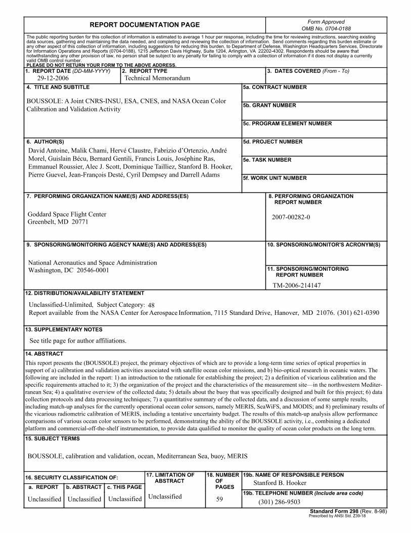
Goddard Space Flight CenterGreenbelt, MD 20771
National Aeronautics and Space AdministrationWashington, DC 20546-0001
Unclassified-Unlimited, Subject Category:Report available from the NASA Center for Aerospace Information, 7115 Standard Drive, Hanover, MD 21076. (301) 621-0390
Unclassified Unclassified Unclassified Unclassified
This report presents the (BOUSSOLE) project, the primary objectives of which are to provide a long-term time series of optical properties in support of a) calibration and validation activities associated with satellite ocean color missions, and b) bio-optical research in oceanic waters. The following are included in the report: 1) an introduction to the rationale for establishing the project; 2) a definition of vicarious calibration and the specific requirements attached to it; 3) the organization of the project and the characteristics of the measurement site—in the northwestern Mediter-ranean Sea; 4) a qualitative overview of the collected data; 5) details about the buoy that was specifically designed and built for this project; 6) data collection protocols and data processing techniques; 7) a quantitative summary of the collected data, and a discussion of some sample results, including match-up analyses for the currently operational ocean color sensors, namely MERIS, SeaWiFS, and MODIS; and 8) preliminary results of the vicarious radiometric calibration of MERIS, including a tentative uncertainty budget. The results of this match-up analysis allow performance comparisons of various ocean color sensors to be performed, demonstrating the ability of the BOUSSOLE activity, i.e., combining a dedicated platform and commercial-off-the-shelf instrumentation, to provide data qualified to monitor the quality of ocean color products on the long term.
BOUSSOLE: A Joint CNRS-INSU, ESA, CNES, and NASA Ocean Color Calibration and Validation Activity
David Antoine, Malik Chami, Hervé Claustre, Fabrizio d’Ortenzio, André Morel, Guislain Bécu, Bernard Gentili, Francis Louis, Joséphine Ras, Emmanuel Roussier, Alec J. Scott, Dominique Tailliez, Stanford B. Hooker, Pierre Guevel, Jean-François Desté, Cyril Dempsey and Darrell Adams
2007-00282-0
TM-2006-214147
See title page for author affiliations.
BOUSSOLE, calibration and validation, ocean, Mediterranean Sea, buoy, MERIS
59
Stanford B. Hooker
(301) 286-9503
Technical Memorandum29-12-2006
48