Boyce/DiPrima 9th ed, Ch 7.5: Homogeneous Linear Systems with Constant CoefficientsElementary Differential Equations and Boundary Value Problems, 9th edition, by William E. Boyce and Richard C. DiPrima, ©2009 by John Wiley & Sons, Inc.

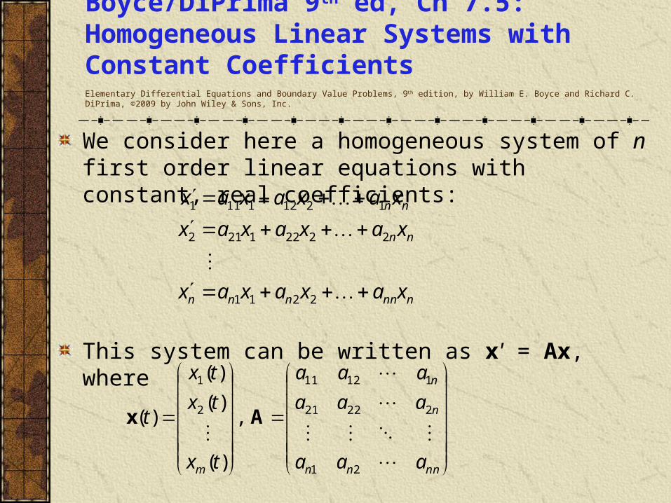
We consider here a homogeneous system of n first order linear equations with constant, real coefficients:

This system can be written as x' = Ax, wherennnnnn

nn

nn

xaxaxax

xaxaxax

xaxaxax

2211

22221212

12121111

nnnn

n

n

m aaa

aaa

aaa

tx

tx

tx

t

21

22221

11211

2

1

,

)(

)(

)(

)( Ax

Equilibrium Solutions

Note that if n = 1, then the system reduces to

Recall that x = 0 is the only equilibrium solution if a 0.

Further, x = 0 is an asymptotically stable solution if a < 0, since other solutions approach x = 0 in this case.

Also, x = 0 is an unstable solution if a > 0, since other solutions depart from x = 0 in this case.

For n > 1, equilibrium solutions are similarly found by solving Ax = 0. We assume detA 0, so that x = 0 is the only solution. Determining whether x = 0 is asymptotically stable or unstable is an important question here as well.

atetxaxx )(

Phase Plane

When n = 2, then the system reduces to

This case can be visualized in the x1x2-plane, which is called the phase plane.

In the phase plane, a direction field can be obtained by evaluating Ax at many points and plotting the resulting vectors, which will be tangent to solution vectors.

A plot that shows representative solution trajectories is called a phase portrait.

Examples of phase planes, directions fields and phase portraits will be given later in this section.

2221212

2121111

xaxax

xaxax

Solving Homogeneous System

To construct a general solution to x' = Ax, assume a solution of the form x = ert, where the exponent r and the constant vector are to be determined.

Substituting x = ert into x' = Ax, we obtain

Thus to solve the homogeneous system of differential equations x' = Ax, we must find the eigenvalues and eigenvectors of A.

Therefore x = ert is a solution of x' = Ax provided that r is an eigenvalue and is an eigenvector of the coefficient matrix A.

0ξIAAξξAξξ rreer rtrt

Example 1: Direction Field (1 of 9)

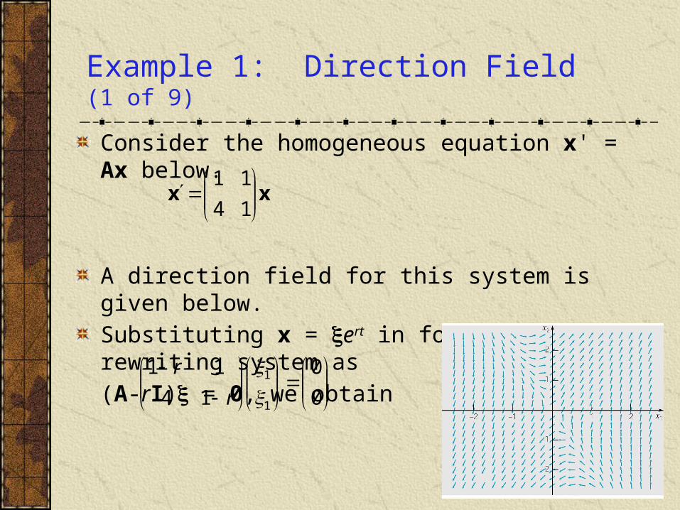
Consider the homogeneous equation x' = Ax below.

A direction field for this system is given below.

Substituting x = ert in for x, and rewriting system as

(A-rI) = 0, we obtain

xx

14

11

0

0

14

11

1

1

r

r

Example 1: Eigenvalues (2 of 9)

Our solution has the form x = ert, where r and are found by solving

Recalling that this is an eigenvalue problem, we determine r by solving det(A-rI) = 0:

Thus r1 = 3 and r2 = -1.

0

0

14

11

1

1

r

r

)1)(3(324)1(14

11 22

rrrrr

r

r

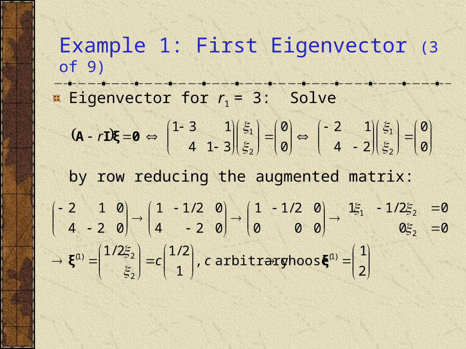
Example 1: First Eigenvector (3 of 9)

Eigenvector for r1 = 3: Solve

by row reducing the augmented matrix:

0

0

24

12

0

0

314

131

2

1

2

1

0ξIA r

2

1choosearbitrary,

1

2/12/1

00

02/11

000

02/11

024

02/11

024

012

)1(

2

2)1(

2

21

ξξ cc

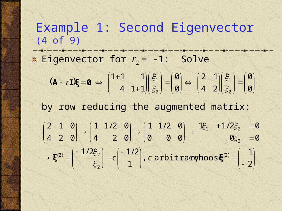
Example 1: Second Eigenvector (4 of 9)

Eigenvector for r2 = -1: Solve

by row reducing the augmented matrix:

0

0

24

12

0

0

114

111

2

1

2

1

0ξIA r

2

1choosearbitrary,

1

2/12/1

00

02/11

000

02/11

024

02/11

024

012

)2(

2

2)2(

2

21

ξξ cc

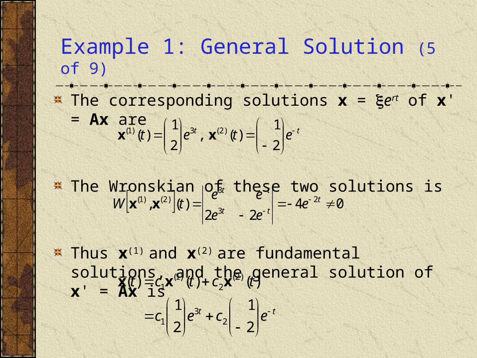
Example 1: General Solution (5 of 9)

The corresponding solutions x = ert of x' = Ax are

The Wronskian of these two solutions is

Thus x(1) and x(2) are fundamental solutions, and the general solution of x' = Ax is

tt etet

2

1)(,

2

1)( )2(3)1( xx

0422

)(, 2

3

3)2()1(

t

tt

tt

eee

eetW xx

tt ecec

tctct

2

1

2

1

)()()(

23

1

)2(2

)1(1 xxx

Example 1: Phase Plane for x(1) (6 of 9)

To visualize solution, consider first x = c1x(1):

Now

Thus x(1) lies along the straight line x2 = 2x1, which is the line through origin in direction of first eigenvector (1)

If solution is trajectory of particle, with position given by

(x1, x2), then it is in Q1 when c1 > 0, and in Q3 when c1 < 0.

In either case, particle moves away from origin as t increases.

ttt ecxecxecx

xt 3

123

113

12

1)1( 2,2

1)(

x

121

2

1

13312

311 2

22, xx

c

x

c

xeecxecx ttt

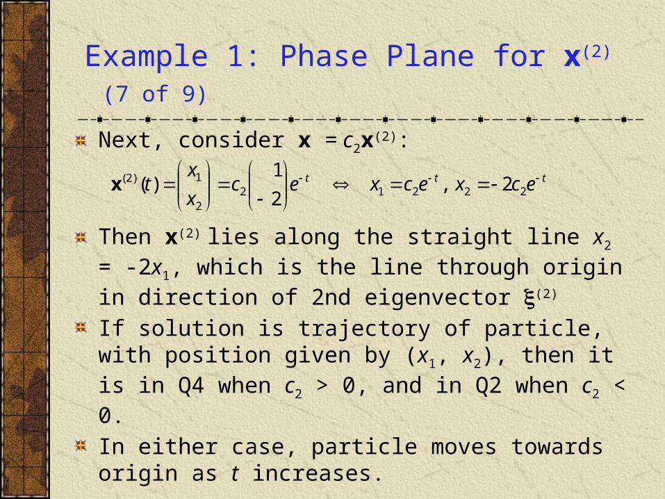
Example 1: Phase Plane for x(2) (7 of 9)

Next, consider x = c2x(2):

Then x(2) lies along the straight line x2 = -2x1, which is the line through origin in direction of 2nd eigenvector (2)

If solution is trajectory of particle, with position given by (x1, x2), then it is in Q4 when c2 > 0, and in Q2 when c2 < 0.

In either case, particle moves towards origin as t increases.

ttt ecxecxecx

xt

22212

2

1)2( 2,2

1)(x

Example 1: Phase Plane for General Solution (8 of 9)

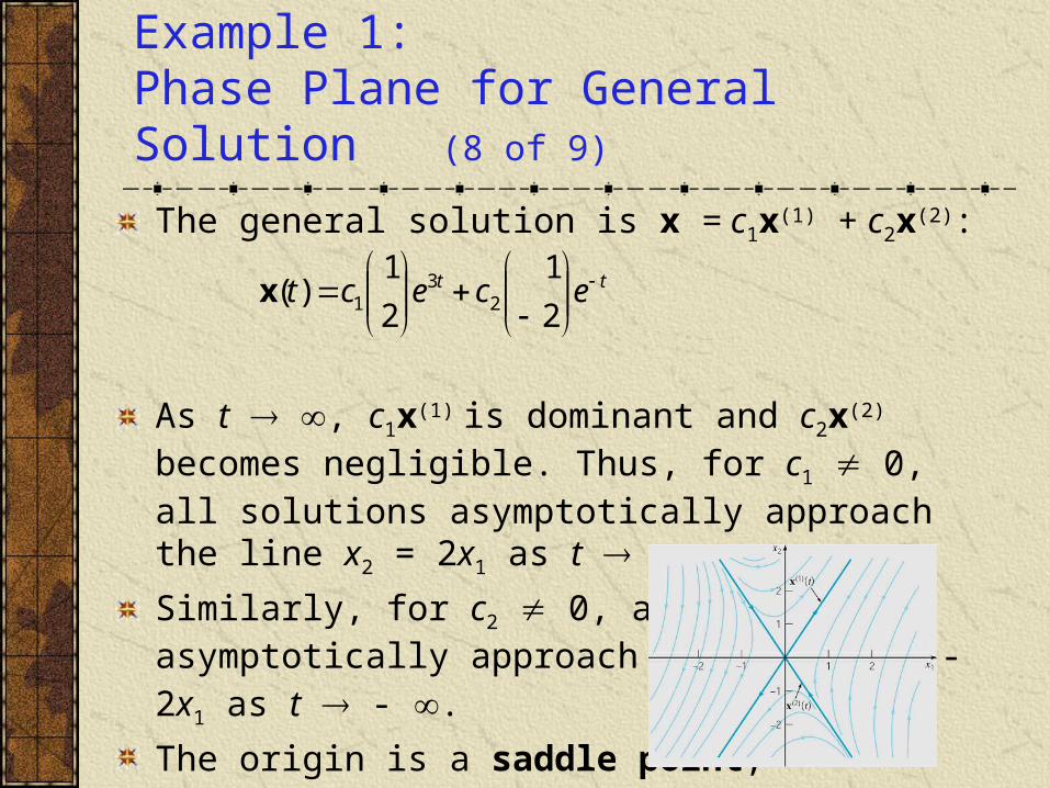
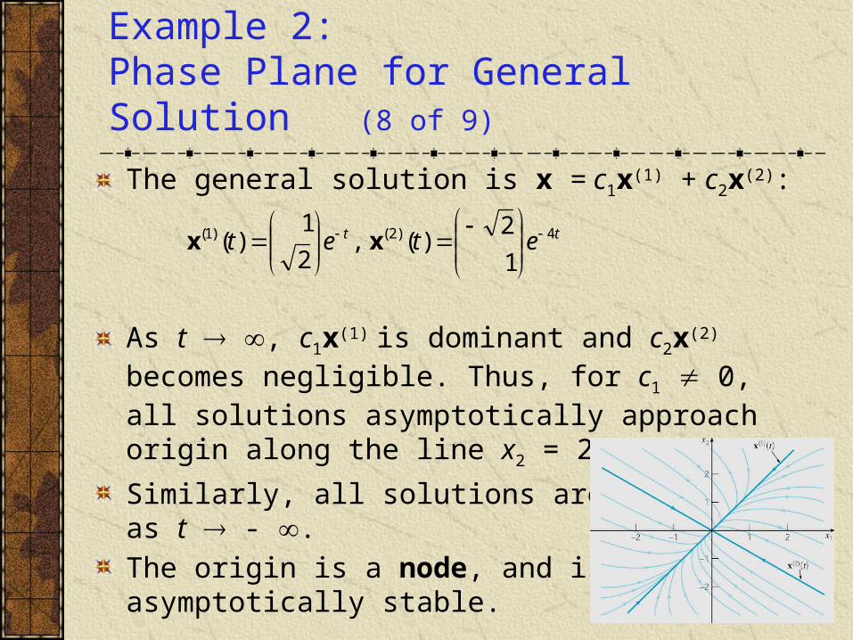
The general solution is x = c1x(1) + c2x(2):

As t , c1x(1) is dominant and c2x(2) becomes negligible. Thus, for c1 0, all solutions asymptotically approach the line x2 = 2x1 as t .

Similarly, for c2 0, all solutions asymptotically approach the line x2 = -2x1 as t - .

The origin is a saddle point,

and is unstable. See graph.

tt ecect

2

1

2

1)( 2

31x

Example 1: Time Plots for General Solution (9 of 9)

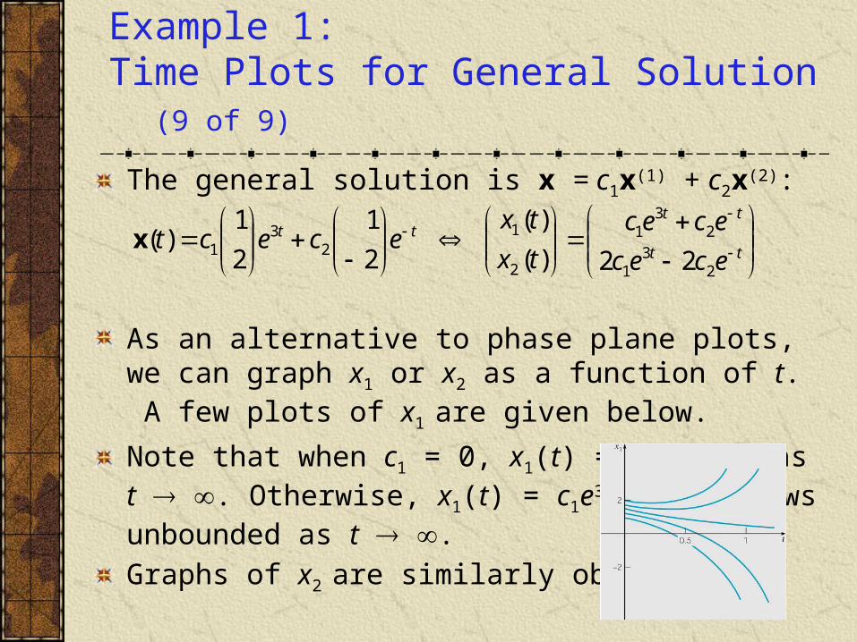
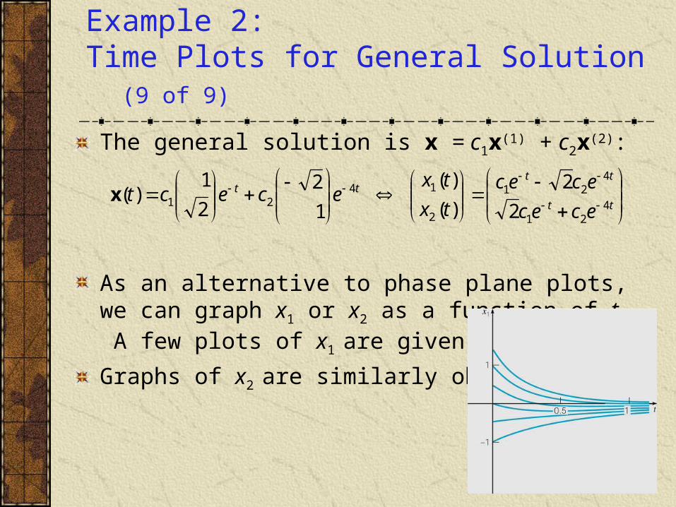
The general solution is x = c1x(1) + c2x(2):

As an alternative to phase plane plots, we can graph x1 or x2 as a function of t. A few plots of x1 are given below.

Note that when c1 = 0, x1(t) = c2e-t 0 as t . Otherwise, x1(t) = c1e3t + c2e-t grows unbounded as t .

Graphs of x2 are similarly obtained.

tt

tttt

ecec

ecec

tx

txecect

23

1

23

1

2

12

31

22)(

)(

2

1

2

1)(x

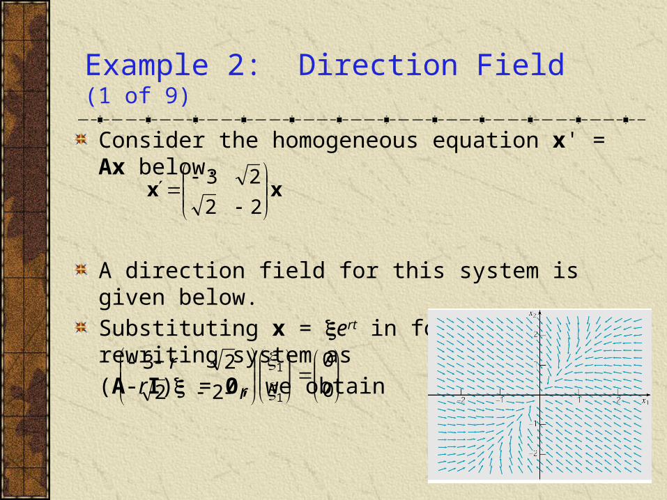
Example 2: Direction Field (1 of 9)

Consider the homogeneous equation x' = Ax below.

A direction field for this system is given below.

Substituting x = ert in for x, and rewriting system as

(A-rI) = 0, we obtain

xx

22

23

0

0

22

23

1

1

r

r

Example 2: Eigenvalues (2 of 9)

Our solution has the form x = ert, where r and are found by solving

Recalling that this is an eigenvalue problem, we determine r by solving det(A-rI) = 0:

Thus r1 = -1 and r2 = -4.

)4)(1(452)2)(3(22

23 2

rrrrrr

r

r

0

0

22

23

1

1

r

r

Example 2: First Eigenvector (3 of 9)

Eigenvector for r1 = -1: Solve

by row reducing the augmented matrix:

0

0

12

22

0

0

122

213

2

1

2

1

0ξIA r

2

1choose

2/2

000

02/21

012

02/21

012

022

)1(

2

2)1( ξξ

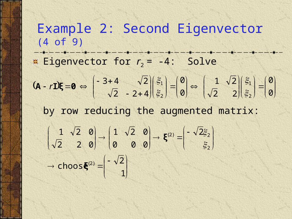
Example 2: Second Eigenvector (4 of 9)

Eigenvector for r2 = -4: Solve

by row reducing the augmented matrix:

0

0

22

21

0

0

422

243

2

1

2

1

0ξIA r

1

2choose

2

000

021

022

021

)2(

2

2)2(

ξ

ξ

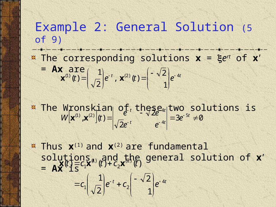
Example 2: General Solution (5 of 9)

The corresponding solutions x = ert of x' = Ax are

The Wronskian of these two solutions is

Thus x(1) and x(2) are fundamental solutions, and the general solution of x' = Ax is

tt etet 4)2()1(

1

2)(,

2

1)(

xx

032

2)(, 5

4

4)2()1(

t

tt

tt

eee

eetW xx

tt ecec

tctct

421

)2(2

)1(1

1

2

2

1

)()()(

xxx

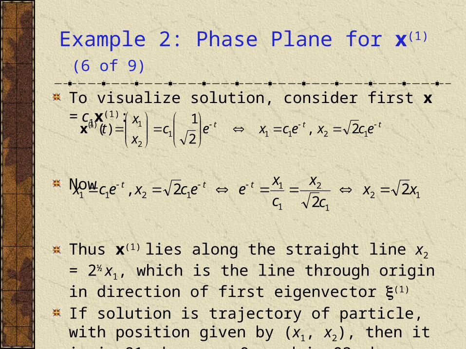
Example 2: Phase Plane for x(1) (6 of 9)

To visualize solution, consider first x = c1x(1):

Now

Thus x(1) lies along the straight line x2 = 2½ x1, which is the line through origin in direction of first eigenvector (1)

If solution is trajectory of particle, with position given by (x1, x2), then it is in Q1 when c1 > 0, and in Q3 when c1 < 0.

In either case, particle moves towards origin as t increases.

ttt ecxecxecx

xt

12111

2

1)1( 2,2

1)(x

12

1

2

1

11211 2

22, xx

c

x

c

xeecxecx ttt

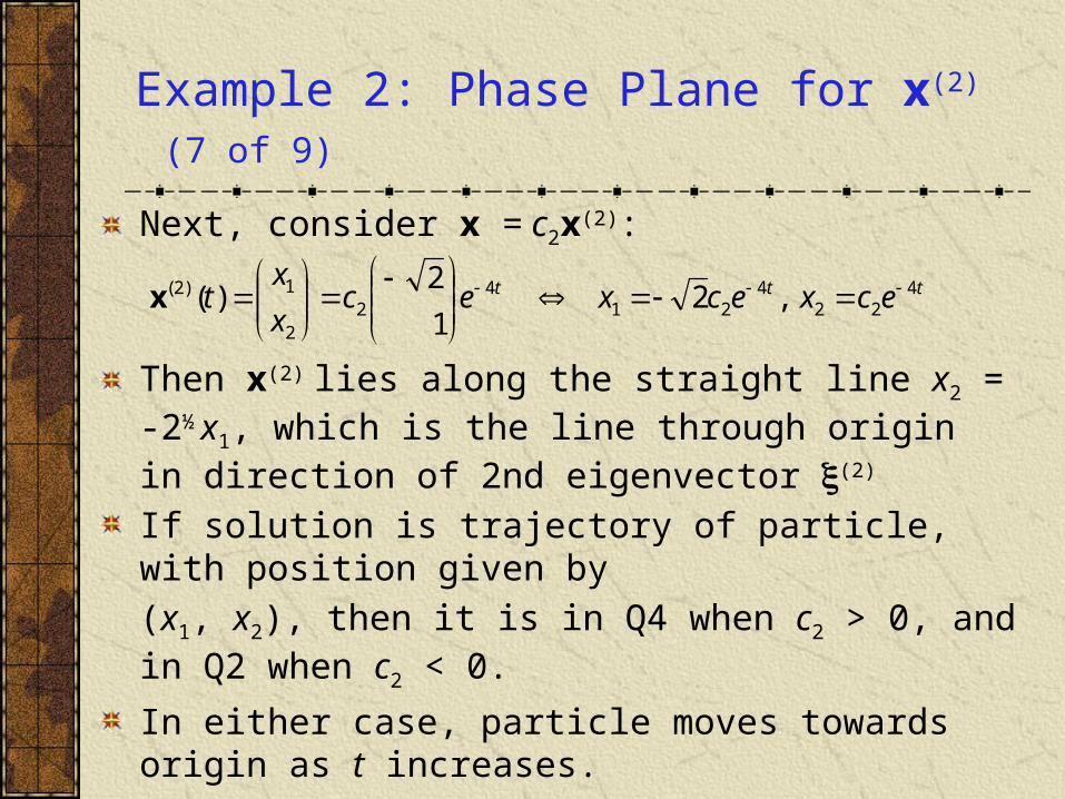
Example 2: Phase Plane for x(2) (7 of 9)

Next, consider x = c2x(2):

Then x(2) lies along the straight line x2 = -2½ x1, which is the line through origin in direction of 2nd eigenvector (2)

If solution is trajectory of particle, with position given by

(x1, x2), then it is in Q4 when c2 > 0, and in Q2 when c2 < 0.

In either case, particle moves towards origin as t increases.

ttt ecxecxecx

xt 4

224

214

22

1)2( ,21

2)(

x

Example 2: Phase Plane for General Solution (8 of 9)

The general solution is x = c1x(1) + c2x(2):

As t , c1x(1) is dominant and c2x(2) becomes negligible. Thus, for c1 0, all solutions asymptotically approach origin along the line x2 = 2½ x1 as t .

Similarly, all solutions are unbounded as t - . The origin is a node, and is asymptotically stable.

tt etet 4)2()1(

1

2)(,

2

1)(

xx

Example 2: Time Plots for General Solution (9 of 9)

The general solution is x = c1x(1) + c2x(2):

As an alternative to phase plane plots, we can graph x1 or x2 as a function of t. A few plots of x1 are given below.

Graphs of x2 are similarly obtained.

tt

tttt

ecec

ecec

tx

txecect

421

421

2

1421

2

2

)(

)(

1

2

2

1)(x

2 x 2 Case: Real Eigenvalues, Saddle Points and Nodes

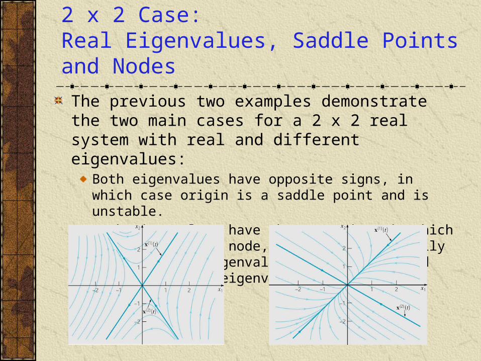
The previous two examples demonstrate the two main cases for a 2 x 2 real system with real and different eigenvalues:

Both eigenvalues have opposite signs, in which case origin is a saddle point and is unstable.

Both eigenvalues have the same sign, in which case origin is a node, and is asymptotically stable if the eigenvalues are negative and unstable if the eigenvalues are positive.

Eigenvalues, Eigenvectors and Fundamental Solutions

In general, for an n x n real linear system x' = Ax:All eigenvalues are real and different from each other.

Some eigenvalues occur in complex conjugate pairs.

Some eigenvalues are repeated.

If eigenvalues r1,…, rn are real & different, then there are n corresponding linearly independent eigenvectors (1),…, (n). The associated solutions of x' = Ax are

Using Wronskian, it can be shown that these solutions are linearly independent, and hence form a fundamental set of solutions. Thus general solution is

trnntr netet )()()1()1( )(,,)( 1 ξxξx

trnn

tr necec )()1(1

1 ξξx

Hermitian Case: Eigenvalues, Eigenvectors & Fundamental Solutions

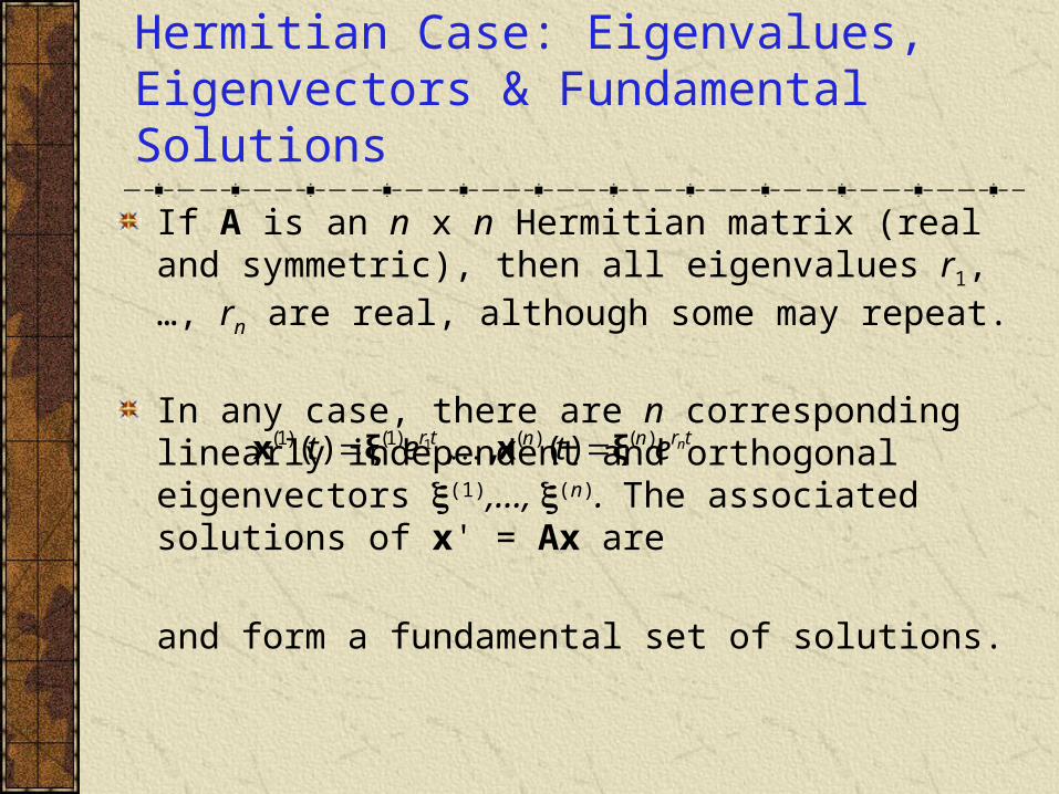
If A is an n x n Hermitian matrix (real and symmetric), then all eigenvalues r1,…, rn are real, although some may repeat.

In any case, there are n corresponding linearly independent and orthogonal eigenvectors (1),…, (n). The associated solutions of x' = Ax are

and form a fundamental set of solutions.

trnntr netet )()()1()1( )(,,)( 1 ξxξx

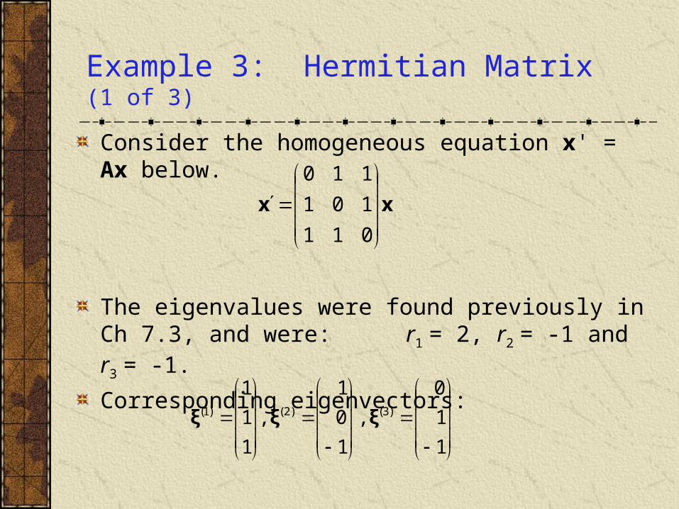
Example 3: Hermitian Matrix (1 of 3)

Consider the homogeneous equation x' = Ax below.

The eigenvalues were found previously in Ch 7.3, and were: r1 = 2, r2 = -1 and r3 = -1.

Corresponding eigenvectors:

xx

011

101

110

1

1

0

,

1

0

1

,

1

1

1)3()2()1( ξξξ

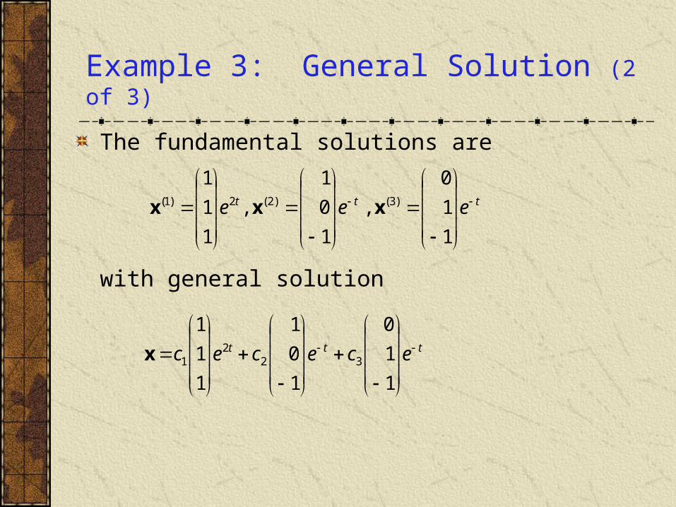
Example 3: General Solution (2 of 3)

The fundamental solutions are

with general solution

ttt eee

1

1

0

,

1

0

1

,

1

1

1)3()2(2)1( xxx

ttt ececec

1

1

0

1

0

1

1

1

1

322

1x

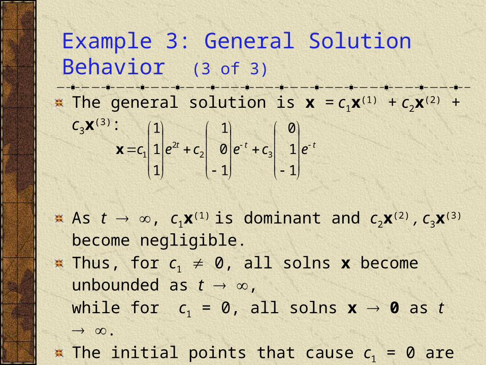
Example 3: General Solution Behavior (3 of 3)

The general solution is x = c1x(1) + c2x(2) + c3x(3):

As t , c1x(1) is dominant and c2x(2) , c3x(3) become negligible.

Thus, for c1 0, all solns x become unbounded as t ,

while for c1 = 0, all solns x 0 as t .

The initial points that cause c1 = 0 are those that lie in plane determined by (2) and (3). Thus solutions that start in this plane approach origin as t .

ttt ececec

1

1

0

1

0

1

1

1

1

322

1x

Complex Eigenvalues and Fundamental Solns

If some of the eigenvalues r1,…, rn occur in complex conjugate pairs, but otherwise are different, then there are still n corresponding linearly independent solutions

which form a fundamental set of solutions. Some may be complex-valued, but real-valued solutions may be derived from them. This situation will be examined in Ch 7.6.

If the coefficient matrix A is complex, then complex eigenvalues need not occur in conjugate pairs, but solutions will still have the above form (if the eigenvalues are distinct) and these solutions may be complex-valued.

,)(,,)( )()()1()1( 1 trnntr netet ξxξx

Repeated Eigenvalues and Fundamental Solns

If some of the eigenvalues r1,…, rn are repeated, then there may not be n corresponding linearly independent solutions of the form

In order to obtain a fundamental set of solutions, it may be necessary to seek additional solutions of another form.

This situation is analogous to that for an nth order linear equation with constant coefficients, in which case a repeated root gave rise solutions of the form

This case of repeated eigenvalues is examined in Section 7.8.

trnntr netet )()()1()1( )(,,)( 1 ξxξx

,,, 2 rtrtrt ettee