Boyd Compressed MAP Quantization 2009

8/3/2019 Boyd Compressed MAP Quantization 2009

http://slidepdf.com/reader/full/boyd-compressed-map-quantization-2009 1/4

IEEE SIGNAL PROCESSING LETTERS, VOL. 17, NO. 2, FEBRUARY 2010 149

Compressed Sensing With Quantized MeasurementsArgyrios Zymnis, Stephen Boyd, and Emmanuel Candès

Abstract—We consider the problem of estimating a sparse signalfrom a set of quantized, Gaussian noise corrupted measurements,

where each measurement corresponds to an interval of values.We give two methods for (approximately) solving this problem,each based on minimizing a differentiable convex function plusan

1

regularization term. Using a first order method developedby Hale et al, we demonstrate the performance of the methodsthrough numerical simulation. We find that, using these methods,compressed sensing can be carried out even when the quantizationis very coarse, e.g., 1 or 2 bits per measurement.

IndexTerms—Compressed sensing,1

, quantized measurement.

I. INTRODUCTION

WE consider the problem of estimating a sparse vector

from a set of noise corrupted quantizedmeasurements, where the quantizer gives us an interval for eachnoise corrupted measurement. We give two methods for solvingthis problem, each of which reduces to solving an regularizedconvex optimization problem of the form

(1)

where is a separable convex differentiable function (whichdepends on the method and the particular measurements),

is the measurement matrix, and is a positive weight

chosen to control the sparsity of the estimated value of .We describe the two methods below, in decreasing order of

sophistication. Our first method is -regularized maximumlikelihood estimation. When the noise is Gaussian (or any otherlog-concave distribution), the negative log-likelihood functionfor , given the measurements, is convex, so computing themaximum likelihood estimate of is a convex optimizationproblem; we then add regularization to obtain a sparseestimate. The second method is quite simple: We simply usethe midpoint, or centroid, of the interval, as if the measurementmodel were linear. We will see that both methods work supris-ingly well, with the first method sometimes outperforming thesecond.

The idea of regularization to encourage sparsity is nowwell established in the signal processing and statistics commu-nities. It is used as a signal recovery method from incomplete

Manuscript received September 16, 2009; revised October 22, 2009. FirstpublishedOctober 30, 2009; current version publishedNovember 18, 2009. Theassociate editor coordinating the review of this manuscript and approving it forpublication was Prof. Markku Renfors.

A. Zymnis and S. Boyd are with the Electrical Engineering Department,Stanford University, Stanford CA 94305 USA (e-mail: [email protected];[email protected]).

E. Candès is with the Statistics and Mathematics Departments, Stanford Uni-versity, Stanford CA 94305 USA (e-mail: [email protected]).

Color versions of one or more of the figures in this paper are available onlineat http://ieeexplore.ieee.org.

Digital Object Identifier 10.1109/LSP.2009.2035667

measurements, known as compressed (or compressive) sensing[1]–[4]. The earliest documented use of based signal revoveryis in deconvolution of seismic data [5], [6]. In statistics, the ideaof regularization is used in the well known Lasso algorithm[7] for feature selection. Other uses of based methods includetotal variation denoising in image processing [8], [9], circuit de-sign [10], [11], sparse portfolio optimization [12], and trend fil-tering [13].

Several recent papers address the problem of quantized com-pressed sensing. In [14], the authors consider the extreme caseof sign (i.e., 1-bit) measurements, and propose an algorithmbased on minimizing an -regularized one-sided quadraticfunction. Quantized compressed sensing, where quantizationeffects dominate noise effects, is considered in [15]; the authorspropose a variant of basis pursuit denoising, based on using an

norm rather than an norm, and prove that the algorithmperformance improves with larger . In [16], an adaptationof basis pursuit denoising and subspace sampling is proposedfor dealing with quantized measurements. In all of this work,the focus is on the effect of quantization; in this paper, weconsider the combined affect of quantization and noise. Still,some of the methods described above, in particular the useof a one-sided quadratic penalty function, are closely relatedto the methods we propose here. In addition, several of theseauthors observed very similar results to ours, in particular, thatcompressed sensing can be successfully done even with verycoarsely quantized measurements.

II. SETUP

We assume that , where is the noisecorrupted but unquantized measurement vector, ,and are IID noises. The quantizer for is given bya function , where is a finite set of codewords.The quantized noise corrupted measurements are

This is the same as saying that .

We will consider the case when the quantizer codewords cor-respond to intervals, i.e., . (Here we includethe lower limit but not the upper limit; but whether the endpointsare included or not will not matter.) The values and are thelower and upper limits, or thresholds, associated with the par-ticular quantized measurement . We can have , or

, when the interval is infinite.Thus, our measurements tell us that

where and are the lower and upper limits for the observedcodewords. This model is very similar to the one used in [17]

for quantized measurements in the context of fault estimation.

1070-9908/$26.00 © 2009 IEEE



150 IEEE SIGNAL PROCESSING LETTERS, VOL. 17, NO. 2, FEBRUARY 2010

III. METHODS

A. -Regularized Maximum Likelihood

The conditional probability of the measured codewordgiven is

where is the th row of and

is the cumulative distribution function of the standard normaldistribution. The negative log-likelihood of given is givenby

which we can express as , where

(This depends on the particular measurement observed throughand .)The negative log-likelihood function is a smooth convex

function. This follows from concavity, with respect to the vari-able , of

where . (This is the log of the probability that anrandom variable lies in .) Concavity of follows fromlog-concavity of , which is the convolu-tion of two log-concave functions (the Gaussian density and thefunction that is one between and and zero elsewhere); see,e.g., [18, Sec. 3.5.2]. This argument shows that is convexfor any measurement noise density that is log-concave.

We find the maximum likelihood estimate of by minimizing. To incorporate the sparsity prior, we add regular-

ization, and minimize , adjusting to obtainthe desired or assumed sparsity in .

We can also add a prior on the vector , and carry out max-imum a posteriori probability estimation. The function

where is the prior density of , is the negative log poste-rior density, plus a constant. Provided the prior density onis log-concave, this function is convex; its minimizer gives themaximum a posteriori probability (MAP) estimate of . Adding

regularization we can trade off posterior probability withsparsity in .

B. -Regularized Least Squares

The second method we consider is simpler, and is based onignoring the quantization. We simply use a real value for each

quantization interval, and assume that the real value is the un-quantized, but noise corrupted measurement. For the measure-

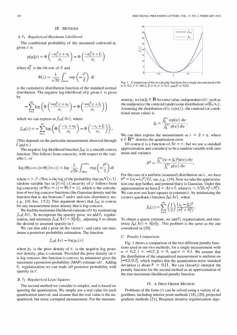
Fig. 1. Comparison of the two penalty functions for a single measurement withu = 0 : 2 , l = 0 0 : 2 , ~ y = 0 , = 0 : 1 , and ~ = 0 : 1 1 .

ment , we let besome value,independent of , such asthe midpointor the centroid (undersome distribution) of .Assuming the distribution of is , the centroid (or condi-tional mean value) is

We can then express the measurement as , wheredenotes the quantization error.

Of course is a function of ; but we use a standardapproximation and consider to be a random variable with zeromean and variance

For the case of a uniform (assumed) distribution on , we have; see, e.g., [19]. Now we take the approxima-tion one step further, and pretend that is Gaussian. Under thisapproximation we have , where .We can now use least-squares to estimate , by minimizing the(convex quadratic) function , where

To obtain a sparse estimate, we add regularization, and min-imize . This problem is the same as the oneconsidered in [20].

C. Penalty Comparison

Fig. 1 shows a comparison of the two different penalty func-tions used in our two methods, for a single measurement with

, , , and . We assume thatthe distribution of the unquantized measurement is uniform on

, which implies that the quantization noise standarddeviation is about . We can (loosely) interpret thepenalty function for the second method as an approximation of the true maximum-likelihood penalty function.

IV. A FIRST ORDER METHOD

Problems of the form (1) can be solved using a variety of al-

gorithms, including interior point methods [18], [20], projectedgradient methods [21], Bregman iterative regularization algo-



ZYMNIS et al.: COMPRESSED SENSING WITH QUANTIZED MEASUREMENTS 151

rithms [22], [23], homotopy methods [24], [25], and a first ordermethod based on Nesterov’s work [26]. Some of these methodsuse a homotopy or continuation algorithm, and so efficientlycompute a good approximation of the regularization path, i.e.,the solution of problem (1) as varies.

We describe here a simple first order method due to Hale et

al.[27], which is a special case of a forward-backward splitting

algorithm for solving convex problems [28], [29]. We start fromthe optimality conditions for (1). Using subdifferential calculus,we obtain the following necessary and sufficient conditions for

to be optimal for (1):

,

,

,

(2)

These optimality conditions tell us in particular that isoptimal for (1) if and only if

(3)

We make use of this fact when selecting the initial value of for our algorithm.

From (2) we deduce that for any , is optimal if andonly if

(4)where and are the elementwise sign and nonneg-ative part operators respectively, and denotes the Hadamard(elementwise) product.

From (4) we see that is optimal if and only if it is a fixedpoint of the following iteration:

(5)

In [27], the authors prove that this iteration converges to an op-timal point of problem (1), starting from an arbitrary point

, as long as the largest eigenvalue of , theHessian of , isbounded. Thisconditionholdsin particularfor both and , since and .

The fixed point continuation method is summarized as fol-lows:

given tolerance , parameters ,

initialize , ,

while

while

For more details about this algorithm, as well as a conver-gence proof, see [27].

For completeness we give for each of the two penalty

functions that we consider. For the negative log-likelihood wehave

where , , . For

the quadratic penalty we have

We found that the parameter values

work well for a large number of problems.

V. NUMERICAL RESULTS

We now look at a numerical example with variablesand up to measurements. For all our simulations, weuse a fixed matrix whose elements are drawn randomly froma distribution. For each individual simulation runwe choose the elements of randomly with

with probability 0.05,

with probability 0.05,

with probability 0.90.

Thus the expected number of nonzeros in is 25, and haszero mean and standard deviation 0.316. The noise standard de-viation is for all , so the signal-to-noise ratio of eachunquantized measurement is about 3.16.

We consider a number of possible measurement scenarios.

We vary , the number of quantization bins used from, 2 to22 and , the number of measurements, from 50 to 500. Wechoose the bin thresholds so as to make each bin have approxi-mately equal probability, assuming a Gaussian distribution. Foreach estimation scenario we use each of the two penalty func-tions described in Section III. For the case of -regularized leastsquares we set the approximation to be the approximate cen-troid of , assuming has distribution ( which itdoes not). In both cases we choose so that has 25 nonzeros,which is the expected number of nonzeros in . So here we areusing some prior information about the (expected) sparsity of to choose .

We generate 100 random instances of and , while keepingfixed, and we record the average percentage of true positive

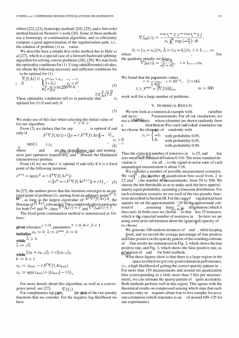
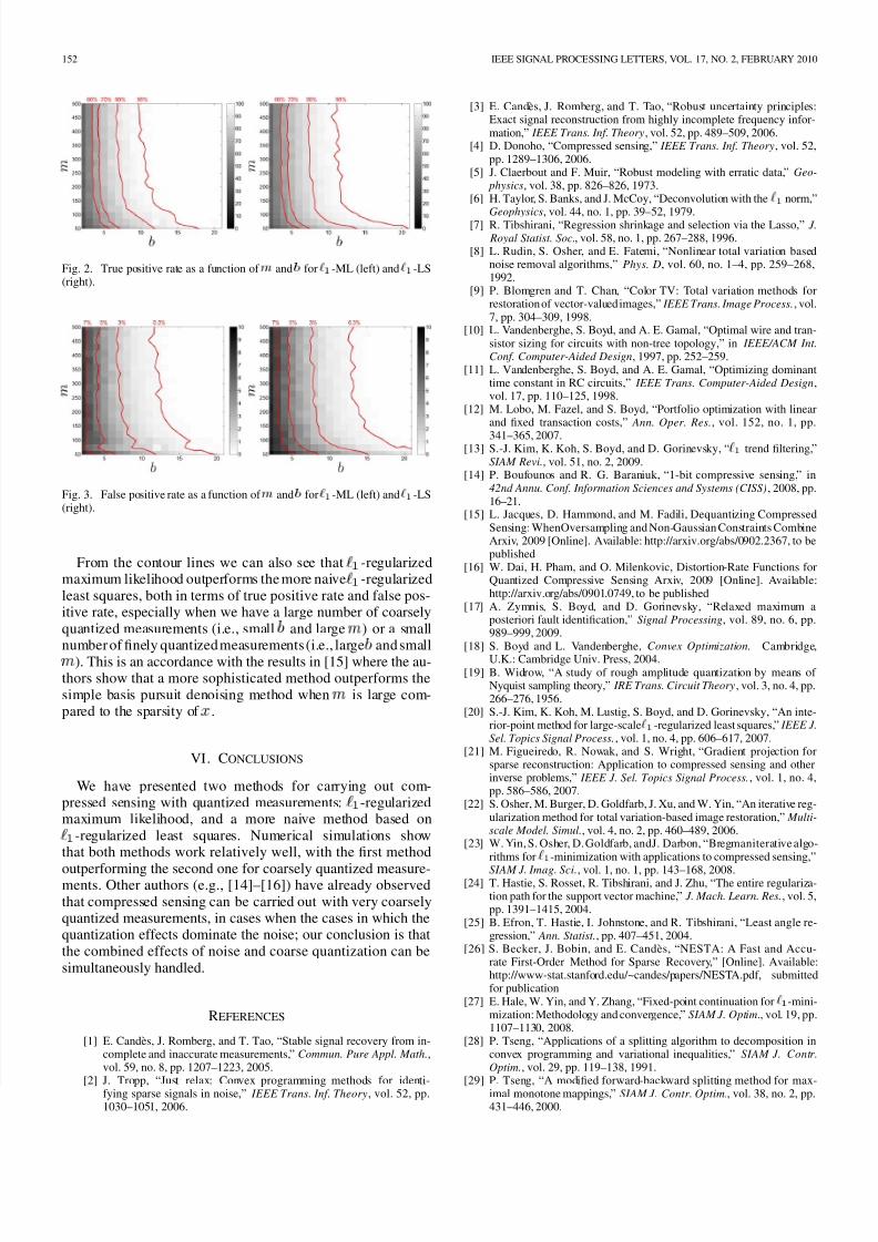
and false positive in the sparsity pattern of the resulting estimateof . Our results are summarized in Fig. 2, which shows the truepositive rate, and Fig. 3, which shows the false positive rate, asa function of and for both methods.

What these figures show is that there is a large region in thespace in which we get very good estimation performance,

i.e., a high likelihood of getting the correct sparsity pattern in .For more than 150 measurements and around ten quantizationbins (corresponding to a little more than 3 bits per measure-ment), we can estimate the sparity pattern of quite accurately.Both methods perform well in this region. This agrees with thetheoretical results on compressed sensing which state that eachnonzero entry in requires about four to five samples for accu-

rate estimation (which translates to an of around 100–125 forour experiments).



152 IEEE SIGNAL PROCESSING LETTERS, VOL. 17, NO. 2, FEBRUARY 2010

Fig. 2. True positive rate as a function of m and b for ̀ -ML (left) and ̀ -LS(right).

Fig. 3. False positive rate as a function of m and b for ̀ -ML (left) and ̀ -LS(right).

From the contour lines we can also see that -regularizedmaximum likelihood outperforms the more naive -regularizedleast squares, both in terms of true positive rate and false pos-itive rate, especially when we have a large number of coarselyquantized measurements (i.e., small and large ) or a smallnumber of finely quantized measurements (i.e., large and small

). This is an accordance with the results in [15] where the au-thors show that a more sophisticated method outperforms thesimple basis pursuit denoising method when is large com-pared to the sparsity of .

VI. CONCLUSIONS

We have presented two methods for carrying out com-pressed sensing with quantized measurements: -regularizedmaximum likelihood, and a more naive method based on

-regularized least squares. Numerical simulations showthat both methods work relatively well, with the first method

outperforming the second one for coarsely quantized measure-ments. Other authors (e.g., [14]–[16]) have already observedthat compressed sensing can be carried out with very coarselyquantized measurements, in cases when the cases in which thequantization effects dominate the noise; our conclusion is thatthe combined effects of noise and coarse quantization can besimultaneously handled.

REFERENCES

[1] E. Candès, J. Romberg, and T. Tao, “Stable signal recovery from in-complete and inaccurate measurements,” Commun. Pure Appl. Math.,vol. 59, no. 8, pp. 1207–1223, 2005.

[2] J. Tropp, “Just relax: Convex programming methods for identi-fying sparse signals in noise,” IEEE Trans. Inf. Theory, vol. 52, pp.1030–1051, 2006.

[3] E. Candès, J. Romberg, and T. Tao, “Robust uncertainty principles:Exact signal reconstruction from highly incomplete frequency infor-mation,” IEEE Trans. Inf. Theory, vol. 52, pp. 489–509, 2006.

[4] D. Donoho, “Compressed sensing,” IEEE Trans. Inf. Theory, vol. 52,pp. 1289–1306, 2006.

[5] J. Claerbout and F. Muir, “Robust modeling with erratic data,” Geo-

physics, vol. 38, pp. 826–826, 1973.[6] H. Taylor, S. Banks, and J. McCoy, “Deconvolution with the ̀ norm,”

Geophysics, vol. 44, no. 1, pp. 39–52, 1979.[7] R. Tibshirani, “Regression shrinkage and selection via the Lasso,” J.

Royal Statist. Soc., vol. 58, no. 1, pp. 267–288, 1996.[8] L. Rudin, S. Osher, and E. Fatemi, “Nonlinear total variation based

noise removal algorithms,” Phys. D, vol. 60, no. 1–4, pp. 259–268,1992.

[9] P. Blomgren and T. Chan, “Color TV: Total variation methods forrestoration of vector-valued images,” IEEE Trans. Image Process., vol.7, pp. 304–309, 1998.

[10] L. Vandenberghe, S. Boyd, and A. E. Gamal, “Optimal wire and tran-sistor sizing for circuits with non-tree topology,” in IEEE/ACM Int.

Conf. Computer-Aided Design, 1997, pp. 252–259.[11] L. Vandenberghe, S. Boyd, and A. E. Gamal, “Optimizing dominant

time constant in RC circuits,” IEEE Trans. Computer-Aided Design,vol. 17, pp. 110–125, 1998.

[12] M. Lobo, M. Fazel, and S. Boyd, “Portfolio optimization with linearand fixed transaction costs,” Ann. Oper. Res., vol. 152, no. 1, pp.

341–365, 2007.[13] S.-J. Kim, K. Koh, S. Boyd, and D. Gorinevsky, “̀ trend filtering,”

SIAM Revi., vol. 51, no. 2, 2009.[14] P. Boufounos and R. G. Baraniuk, “1-bit compressive sensing,” in

42nd Annu. Conf. Information Sciences and Systems (CISS) , 2008, pp.16–21.

[15] L. Jacques, D. Hammond, and M. Fadili, Dequantizing CompressedSensing: WhenOversampling and Non-Gaussian Constraints CombineArxiv, 2009 [Online]. Available: http://arxiv.org/abs/0902.2367, to bepublished

[16] W. Dai, H. Pham, and O. Milenkovic, Distortion-Rate Functions forQuantized Compressive Sensing Arxiv, 2009 [Online]. Available:http://arxiv.org/abs/0901.0749, to be published

[17] A. Zymnis, S. Boyd, and D. Gorinevsky, “Relaxed maximum aposteriori fault identification,” Signal Processing, vol. 89, no. 6, pp.989–999, 2009.

[18] S. Boyd and L. Vandenberghe , Convex Optimization. Cambridge,U.K.: Cambridge Univ. Press, 2004.

[19] B. Widrow, “A study of rough amplitude quantization by means of Nyquist sampling theory,” IRE Trans. Circuit Theory, vol. 3, no. 4, pp.266–276, 1956.

[20] S.-J. Kim, K. Koh, M. Lustig, S. Boyd, and D. Gorinevsky, “An inte-rior-point method for large-scale ̀ -regularized least squares,” IEEE J.

Sel. Topics Signal Process., vol. 1, no. 4, pp. 606–617, 2007.[21] M. Figueiredo, R. Nowak, and S. Wright, “Gradient projection for

sparse reconstruction: Application to compressed sensing and otherinverse problems,” IEEE J. Sel. Topics Signal Process., vol. 1, no. 4,pp. 586–586, 2007.

[22] S. Osher, M. Burger, D. Goldfarb, J. Xu, and W. Yin, “An iterative reg-ularization method for total variation-based image restoration,” Multi-

scale Model. Simul., vol. 4, no. 2, pp. 460–489, 2006.[23] W. Yin, S. Osher, D. Goldfarb, andJ. Darbon, “Bregmaniterative algo-

rithms for ̀ -minimization with applications to compressed sensing,”

SIAM J. Imag. Sci., vol. 1, no. 1, pp. 143–168, 2008.[24] T. Hastie, S. Rosset, R. Tibshirani, and J. Zhu, “The entire regulariza-

tion path for the support vector machine,” J. Mach. Learn. Res., vol. 5,pp. 1391–1415, 2004.

[25] B. Efron, T. Hastie, I. Johnstone, and R. Tibshirani, “Least angle re-gression,” Ann. Statist., pp. 407–451, 2004.

[26] S. Becker, J. Bobin, and E. Candès, “NESTA: A Fast and Accu-rate First-Order Method for Sparse Recovery,” [Online]. Available:http://www-stat.stanford.edu/~candes/papers/NESTA.pdf, submittedfor publication

[27] E. Hale, W. Yin, and Y. Zhang, “Fixed-point continuation for ̀ -mini-mization: Methodology and convergence,” SIAM J. Optim., vol. 19, pp.1107–1130, 2008.

[28] P. Tseng, “Applications of a splitting algorithm to decomposition inconvex programming and variational inequalities,” SIAM J. Contr.

Optim., vol. 29, pp. 119–138, 1991.[29] P. Tseng, “A modified forward-backward splitting method for max-

imal monotone mappings,” SIAM J. Contr. Optim., vol. 38, no. 2, pp.431–446, 2000.

Documents

Boyd Compressed MAP Quantization 2009