Boynton Inlet Flow Measurement Study · Boynton Inlet Flow Measurement Study ... OAR-AOML-43 May 2013 Atlantic Oceanographic and ... and Lecia Salerno participated in the field efforts

Boynton Inlet Flow Measurement Study

U.S. Department of Commerce | National Oceanic and Atmospheric Administration

NOAA Technical ReportOAR-AOML-43

May 2013

Atlantic Oceanographic and Meteorological LaboratoryMiami, Florida

DisclaimerNOAA does not approve, recommend, or endorse any proprietary product or material mentioned in this document. No reference shall be made to NOAA or to this document in any advertising or sales promotion which would indicate or imply that NOAA approves, recommends, or endorses any proprietary product or proprietary material herein or which has as its purpose any intent to cause directly or indirectly the advertised product to be used or purchased because of this document. The findings and conclusions in this report are those of the authors and do not necessarily represent the view of the funding agency.

Suggested CitationStamates, S.J., 2013: Boynton Inlet flow measurement study. NOAA Technical Report,

OAR‑AOML‑43, 13 pp.

AcknowledgmentsThis work was funded by NOAA’s Atlantic Oceanographic and Meteorological Laboratory in Miami, Florida. Thanks to Dr. John Proni for enabling this project to occur. Madeleine Adler, Joseph Bishop, Cheryl Brown, Hector Casanova, Jules Craynock, Shailer Cummings, Paul Dammann, and Lecia Salerno participated in the field efforts and calibration exercises. Thanks are due to the U.S. Geological Survey for publishing a number of excellent documents relating to flow measurements and, especially, to Victor Levesque for sharing his knowledge and expertise with the author. Thanks are due to Gail Derr for the editing and production of this report.


UNITED STATES DEPARTMENT OF COMMERCEDr. Rebecca A. Blank, Acting Secretary

NATIONAL OCEANIC AND ATMOSPHERIC ADMINISTRATIONDr. Kathryn D. Sullivan, Acting Under Secretary of Commerce forOceans and Atmosphere/NOAA Administrator

S. Jack Stamates

NOAA-Atlantic Oceanographic and Meteorological Laboratory Miami, Florida

OFFICE OF OCEANIC AND ATMOSPHERIC RESEARCHDr. Robert S. Detrick, Assistant Administrator

NOAA Technical ReportOAR-AOML-43

May 2013

This page intentionally left blank.

| iii


NOAA Technical Report, OAR-AOML-43

Table of Contents

Acronyms ............................................................................................................................. iv

Figures .................................................................................................................................. v

Tables .................................................................................................................................... v

Abstract................................................................................................................................ vi

1. Introduction ................................................................................................................... 1

2. Methods ........................................................................................................................ 2

2.1 Index velocity method ....................................................................................... 2 2.2 500‑kHz side‑looking Doppler sonar ................................................................ 3 2.3 Equipment installation ...................................................................................... 3 2.4 Measurement parameters ................................................................................... 4 2.4.1 Sampling interval ................................................................................... 4 2.4.2 Averaging interval .................................................................................. 5 2.4.3 Cell size ................................................................................................. 5 2.5 Equipment service ............................................................................................. 6 2.6 Channel geometry ............................................................................................. 7 2.7 Calibration and calculation of index velocity ..................................................... 8 2.7.1 Calibration system ................................................................................. 8 2.7.2 Calibration data acquisition and processing ........................................... 8

3. Results ............................................................................................................................ 9

3.1 Mean channel velocity and Q estimates ............................................................. 9 3.2 Tidal prism estimates ....................................................................................... 10 3.3 Canal outflow and precipitation ...................................................................... 10 3.4 Effects of wind on tidal prism .......................................................................... 11 3.5 Sources of error ............................................................................................... 12

4. Data Applications ........................................................................................................ 12

4.1 Nutrient flux studies ........................................................................................ 12 4.2 Tracer studies and inlet dispersion modeling .................................................... 13

5. Conclusions .................................................................................................................. 13

6. References .................................................................................................................... 13

| iv



Acronyms

ADCP Acoustic Doppler current profiler

AOML Atlantic Oceanographic and Meteorological Laboratory

Q Transport across a channel cross section per unit of time (m3/s)

SL Side‑looking acoustic Doppler velocity measurement system

| v



Figures

1. Location of the Boynton Inlet ......................................................................................... 1

2. Boynton Inlet at ebb tide with plume .............................................................................. 2

3. Side‑looking acoustic profiler in mounting frame prior to installation ............................. 4

4. Mounting frame installed at the Boynton Inlet ................................................................ 4

5. Multicell data mean and range plots ................................................................................ 6

6a. Side‑looking acoustic profiler after recovery from a deployment ...................................... 6

6b. Refurbished side‑looking acoustic profiler before a deployment ....................................... 6

7. Channel geometry measurements .................................................................................... 7

8. Riverboat platform .......................................................................................................... 8

9. Regression plot of calibration data ................................................................................... 9

10. Time series of velocity data .............................................................................................. 9

11. Histogram of velocity data for a one‑year period .............................................................. 9

12. Histogram of Q rates for a one‑year period .................................................................... 10

13. Histograms of tidal prism for a one‑year period ............................................................. 10

14. Regression of volume per tidal phase with the north wind component .......................... 11

15. Time series of tidal prism and north component of the wind ......................................... 12

16. Time series of tidal prism with north and east components of the wind ......................... 12

Tables

1. Side‑looking acoustic profiler cell locations ...................................................................... 5

2. Statistics of the mean channel velocity and Q for a one‑year period ................................. 9

3. Statistics of the tidal prism for a one‑year period ........................................................... 10

4. Statistics of canal flow and comparison with net outflow through the Boynton Inlet ..... 11

5. Regression statistics of the north and east wind components and tidal prism ................. 11

| vi



AbstractA 500 kHz side‑looking Acoustic Doppler profiler was installed on the north seawall of the Boynton Inlet (26°32.744´N, 80°02.637´W) on February 20, 2007 and remained operational through August 2008. The system measured a profile of velocities across the inlet and also measured the water level above the instrument. Data from this system were calibrated by regressing the velocity data with data from an independent, down‑looking acoustic Doppler profiler which was repeatedly transected across the channel during flood and ebb tidal phases. The down‑looking Doppler system was also used to measure the bathymetric profile of the channel at the location of the measurement system. This information was used to generate estimates of the channel flux at 15‑minute intervals. These flux measurements were integrated over flood and ebb tidal periods to estimate the tidal prism of the inlet. Comparisons of these tidal prism estimates with wind data collected at Lake Worth pier showed that the north component of the wind velocity was correlated with the Boynton Inlet tidal prism.

| 1



1. IntroductionBoynton Inlet, also known as the South Lake Worth Inlet, is located on the southeastern coast of Florida (Figure 1). This inlet is one of two inlets that connect the Lake Worth Lagoon to the Atlantic Ocean (the second being the Palm Beach Inlet). The inlet was constructed in 1927 and has undergone many modifications since that time (South Lake Worth Inlet Management Plan, 1998). Flow through the inlet is principally driven by the local semi‑diurnal tides.

The Lake Worth Lagoon is located in an urbanized area. Several large canals deliver inland waters to the lagoon. These canals are managed as components of the South Florida Water Management District system. The C51 canal, in particular, connects Lake Okeechobee with the Atlantic Ocean via the Boynton and Palm Beach inlets. Along its path, it provides drainage for the sugarcane fields in the Everglades agricultural area and receives storm water runoff from several cities on its way to the Lake Worth Lagoon (Florida Department of Environmental Protection, 1999).

Water in the Lake Worth Lagoon typically has a significantly higher concentration of nutrients than coastal ocean waters (Taylor Engineering, Inc., 2009; Carsey et al., 2012). Twice a day, on the ebb tide, water from the Lake Worth Lagoon flows seaward through the Boynton Inlet into the coastal ocean. These nutrient‑laden waters exiting the inlet into the ocean have the potential to impact the nearshore environment (Figure 2).

A study was conducted in 2007 to quantify the flux of materials through the Boynton Inlet (Carsey et al., 2012); this current project is a component of that study. A side‑looking acoustic Doppler flow measurement system (SL) was installed inside the inlet on February 20, 2007 and provided data until August 2008. This system provided measurements of the water velocity in a section of the inlet at 15‑minute intervals. These velocity measurements were calibrated using data gathered from an independent, down‑looking acoustic Doppler current profiler (ADCP) so that the velocity measured by the SL could be used to estimate the mean channel velocity of the inlet (the mean

Figure 1. Location of the Boynton Inlet on the southeast coast of Florida.

| 2



channel velocity is discussed in section 2.1). The calibrated velocity measurements, in conjunction with knowledge of the channel geometry at the measurement location and a measurement of the water level in the channel, were used to estimate the total volume of water moving through the inlet per unit of time, Q (m3/s). These measurements were integrated over the flood and ebb tidal periods to estimate the total transport through the inlet per tidal phase (tidal prism). The tidal prism estimates were compared with the local winds, and a relationship between the wind and flow through the inlet was calculated. These measurements, in conjunction with a series of nutrient concentration measurements, were used to estimate the flux of certain nutrients through the Boynton Inlet into the coastal ocean.

2. Methods2.1 Index Velocity Method

The application of a SL system to measure the flux across a channel‑cross section (Q) is well documented and referred to as the “index velocity method” (Levesque and Oberg, 2012). This method is often used to measure the flow of a

stream or river. The application of this method to a tidally‑driven inlet presented a few particular challenges (Ruhl and Simpson, 2005).

In the application of this method, an acoustic Doppler measurement device is placed into the channel to make a measurement of the velocity in a portion of the channel. The device is mounted along one side of the channel and profiles the horizontal velocities across the channel. A data value from a section of the horizontal profile is used as a representative velocity. The constraint placed upon this representative velocity measurement is that this velocity must be relatable to the mean channel velocity at the location where the measurement is made. The mean channel velocity (Vmc) is that velocity which, when multiplied by the channel cross‑sectional area (A) at the measurement location, gives the flux across that cross section, Q

Q = A × Vmc (1)

To establish the relationship between the velocity measured by the fixed SL system and the mean channel velocity, an independent, down‑looking ADCP instrument is repeatedly transected across the channel during flood and ebb tides to

Figure 2. Boynton Inlet with a plume exiting the inlet during an ebb tide.

| 3



obtain the flux rates through the channel while the fixed SL system simultaneously makes velocity measurements in the channel. The data from these two systems are then used to develop a relationship that allows the SL system to estimate the mean channel velocity. To estimate the cross‑sectional area of the channel, an accurate description of the channel geometry must be known and the water level in the channel at the time of the measurement must also be known.

2.2 500-kHz Side-Looking Doppler Sonar

The SonTek Argonaut 500‑kHz side‑looking Doppler sonar (SonTek Corporation, 2006) used for this project estimates the velocity of the water flowing through a channel by measuring the Doppler shift returned from acoustic signals transmitted along two paths. For this application, the instrument was mounted on the side of the channel at a depth equal to the mid‑water level in the channel at low tide. The instrument’s central measurement axis pointed across the channel, with the two acoustical transducers pointed at a 25° angle to the left and right of the measurement axis. The instrument was mounted so that the two acoustic beams lay in a horizontal plane relative to the water surface. The system calculated water velocities in the direction of the channel axis and in the direction perpendicular to the channel axis in the plane defined by the acoustic beam paths.

The SL has a feature such that it can be instructed to subdivide the velocity measurements into as many as 11 measurement cells along the measurement axis. In all cases, there is a minimum distance from the instrument to the point where any measurement cell can begin. This is referred to as the blanking distance. This distance relates to the time necessary for the instrument to make the transition from transmission mode to receive mode. The minimum blanking distance for the SonTek 500‑kHz SL is 1.5 m. As many as 10 cells (called multicells) of a user‑defined size can be used to collect a horizontal profile across a distance defined by the blanking distance, the cell size, and the number of cells. The 11th cell, or integrated velocity cell, has its start and end distances set by the user. This cell’s range is independent of the multicells.

The SL is equipped with two methods for measuring the water level above the instrument. The first method uses an acoustic signal transmitted by a transducer mounted on the top of the instrument. By measuring the time between

the transmission of an acoustic pulse and the time that the reflection of that pulse from the water surface is received, the distance to the surface can be calculated. The SL transmits a vertical pulse each time the system transmits a horizontal pulse (as configured, the system transmitted 450 pulses at a 1‑Hz rate in a 7.5‑minute interval). The average of these estimates is reported in each measurement cycle as the distance from the instrument to the (average) water surface. Using an acoustical signal to make a distance measurement requires knowledge of the speed of sound in the water. The sound speed is a function of temperature, salinity, and density of the water (Clay and Medwin, 1977). The SL is equipped with a temperature sensor which is used to correct the sound speed for changing temperature. The salinity value is entered as a constant, and the density is estimated by the device from the salinity constant depth of the instrument and the measured temperature.

The second method for estimating the water level above the instrument is by means of a pressure sensor located on the top of the instrument. This sensor measures the pressure generated by the water above the instrument. As this sensor is not vented to the surface, changes in atmospheric pressure will be reflected in the reading from the pressure sensor. Data from the pressure sensor were used only in cases where the acoustical data were deemed to be inaccurate (3% of the acoustical data were deemed bad and replaced by the pressure data). In the cases where the pressure sensor was used in place of the acoustical sensor, the pressure sensor was brought into alignment with the acoustical sensor using data from the period preceding the loss of the acoustical data, where the data were valid for both sensors.

2.3 Equipment Installation

The measurement system was installed on the north bank of the Boynton Inlet approximately 50 m west of the AIA Bridge at coordinates 26°32.744´N, 80°02.637´W. This location was selected because of the suitability of the seawall structure for mounting the instrument and also because visual observations showed that this part of the channel had the smoothest bottom topography. To mount the SL, a mounting frame (Figure 3) supplied by SonTek was affixed onto the north bulkhead. A piece of sign post attached to the bottom of the frame was driven into the channel bottom to stabilize the frame, and cables were attached between the

| 4



sides of the mounting frame and the seawall to laterally stabilize the mounting (Figure 4).

The platform on which the SL was mounted slides within the mounting frame system and allowed the SL to be raised vertically in the mounting frame without changing the orientation of the SL with respect to its pitch and roll axis. This mounting frame system allowed the SL to be positioned within the water column and allowed the orientation of the SL to be adjusted so that it was perpendicular to the axis of the channel and its acoustic beams made parallel to the water surface. The mounting frame system also allowed the SL to be retrieved for maintenance and data recovery and then redeployed to the same position with excellent repeatability. The depth of the SL was set to be approximately at the mid depth of the channel at low tide. This corresponded to approximately 1.7 m from the channel bottom at the location of the instrument. During the installation process

and during subsequent checks of the system orientation, the SL was operated with a cable coming to the surface so that data could be reviewed in real time to assure the acoustic propagation path was not coming into contact with obstacles, the bottom, or the surface. During deployments, the SL was equipped with an internal memory and external battery pack. This allowed the system to be submerged with no cabling to the surface. The system was programmed to begin data collection at a pre‑determined time and continue recording to the internal memory until the next service interval or until the battery supply was depleted.

2.4 Measurement Parameters

The SL system allows the user to define the sampling parameters and measurement cell size to optimize the deployment for the environment and the desired maintenance interval. After an initial seven day‑deployment, the data were analyzed and the parameters set as follows.

2.4.1 Sampling Interval

The sampling interval was defined as the time interval between measurement cycles. To capture the rapidly‑changing flow conditions at Boynton Inlet while also not depleting the battery supply too quickly, a sampling interval of 15 minutes was selected.

Figure 3. Aragonaut 500-kHz side-looking acoustical profiler and its mounting frame prior to installation in the Boynton Inlet.

Figure 4. The flow measurement system mounted on the north bulkhead of Boynton Inlet.

| 5



2.4.2 Averaging Interval

The averaging interval was defined as that part of the sampling interval where the instrument was actively gathering data. The SonTek SL collected data at a 1‑Hz rate during the averaging interval. The data collected during the averaging interval were averaged and reported at the interval of the sampling interval.

Boynton Inlet is a very dynamic environment, and current velocities can exceed 2 m/s. Oftentimes, there are significant waves in the inlet. For example, when a large vessel passes through the inlet, standing waves can set up in the channel which take on the order of minutes to disperse. These complexities suggest that a long averaging interval should be used. The disadvantage to a longer averaging interval is that the battery will be depleted sooner. After examination of the initial data, an averaging interval of 7.5 minutes (450 s) was selected. As the instrument sampled at the 1‑Hz rate, this resulted in 450 samples being averaged into a measurement that was reported at the sample interval period of 15 minutes (900 s).

To summarize, the instrument was set with a sampling interval of 15 minutes (900 s) and an averaging interval of 7.5 minutes (450 s). When the instrument reached the time for a sampling interval to begin, it collected data at a 1‑Hz rate for 450 seconds. These data were averaged and recorded, and the instrument then waited for the remaining 450 seconds until the next measurement cycle began.

2.4.3 Cell Size

After inspection of the initial data, the position of multicells 1‑10 were set to start at 1.5 m from the transducer (the blanking distance) and have a size of 3.35 m, while the integrated velocity cell was set to measure 7.5‑27.5 m from the instrument. Table 1 provides the beginning and ending distances for each cell from the instrument. Note that the cells were not totally independent. The acoustic return that was attributed to a cell was actually from a triangularly‑weighted cell that was twice the stated cell size. Therefore, water at a distance of one‑half of a cell size before and after the cell affected the reported velocity for that cell, albeit with a weighting function applied. This was taken into account for the choice of the 3.35 m size for cells 1‑10. In this case, the stated cell end for cell 10 was 35 m from the

instrument. However, taking into account the extra half cell that extended past the cell, this put the cell end distance to be 36.675 m. This distance was shorter than the distance to the south wall and, therefore, the 10th cell should not have been influenced by this boundary. From the multicell data and visual observations of the flow patterns in the Boynton Inlet, it was noted that the flow in the channel was not symmetric from side to side and was different on the ebb and flood tides. The average velocity of the multicells and integrated measurement cell derived from all the available data and separated into flood and ebb tidal phases are shown in Figure 5.

During the flood tide, water enters Boynton Inlet through curved jetties and is forced onto the north side of the channel, and the velocities along the north side of the channel remain higher. In Figure 5 it can be observed that the average velocity is highest in cell 2 during the flood tide. During the ebb tide, it was observed that water “wraps around” the south seawall at its western extent. The flow pattern visually appears to move away from the seawall after entering the channel at that point. Figure 5 shows cells 9 and 10 having a markedly lower averaged velocity. This may be a result of the flow of the water around the seawall as mentioned. The initial multicell data were examined for correlation amongst each other on both the flood and ebb tides. From these observations and analysis, it was determined that the distance of 7.5‑27.5 m as measured from the instrument on the north seawall would be the range of the integrated

Table 1. Distance in meters from the instrument to the measurement cells.

CellStart

RangeMiddle

Point Range End

Range

Multicell 1 1.5 3.175 4.85

Multicell 2 4.85 6.525 8.2

Multicell 3 8.2 9.875 11.55

Multicell 4 11.55 13.225 14.9

Multicell 5 14.9 16.575 18.25

Multicell 6 18.25 19.925 21.6

Multicell 7 21.6 23.275 24.95

Multicell 8 24.95 26.625 28.3

Multicell 9 28.3 29.975 31.65

Multicell 10 31.65 33.325 35

Integrated Velocity Cell 7.5 17.5 27.5

| 6



velocity cell. This range corresponded to 53% of the width of the channel. The velocities reported from the integrated measurement cell were then used in further calculations.

2.5 Equipment Service

As configured, the SL had enough power in its battery pack to sample continuously for 33 days. Prior to the depletion of the battery pack, the SL was brought to the surface and refurbished for the next deployment. This involved cleaning the instrument, downloading the data, and installing a fresh battery pack. This could typically be accomplished within one hour, which minimized the time that the SL was not collecting data. The SL would typically become quite fouled with small barnacles and other marine growth during a deployment (Figure 6a). This was especially true during the summer months.

Prior to deploying the SL for the first time, the instrument and the mounting frame assembly were painted with an anti‑fouling coating. After a few months of service, the anti‑fouling coating ceased to prevent marine growth on the instrument. Reapplying the anti‑fouling coating to the SL necessitated removing the instrument from the Boynton Inlet for a period of days, thereby disrupting the data record. This was done once in August 2007. Removing the portion

of the mounting frame that was attached to the inlet seawall for re‑coating was not an option. To mitigate the effects of biofouling without removing the SL from service, a mixture of silicone grease and ground hot chili pepper was applied to the instrument as shown in Figure 6b (Alliance for Coastal Technology, 2005). This coating could be applied on site during instrument service visits and did help prevent (but not eliminate) the accumulation of fouling on the SL during deployments. Being mostly submerged, the mounting structure could not be coated with any such mixture. After

Figure 6b. Acoustic profiler and battery pack after refurbishment and prior to redeployment. Note the mixture of silicone grease and hot chili powder used on the instrument to slow the growth of fouling organisms.

Figure 6a. Acoustic profiler and battery pack after removal from the Boynton Inlet following a 33-day deployment.

Figure 5. Data showing the mean (point), standarad deviation (box), and minimum and maximum values (whisker) from the ten multicells and integrated cell that were used to estimate the mean channel velocity. The bar crossing in front to the ebb and flood cell whiskers indicate the approximate position of the integrated measurement cell.

| 7



about six months, the mounting structure became so fouled that retrieving the instrument was difficult. This necessitated a swimmer to enter the water and clean the mounting by scraping the barnacles from the mounting with a blunt tool so that the SL could be brought to the surface. With the strong water velocities inside the inlet and the very short period of slack currents, this was a challenging procedure.

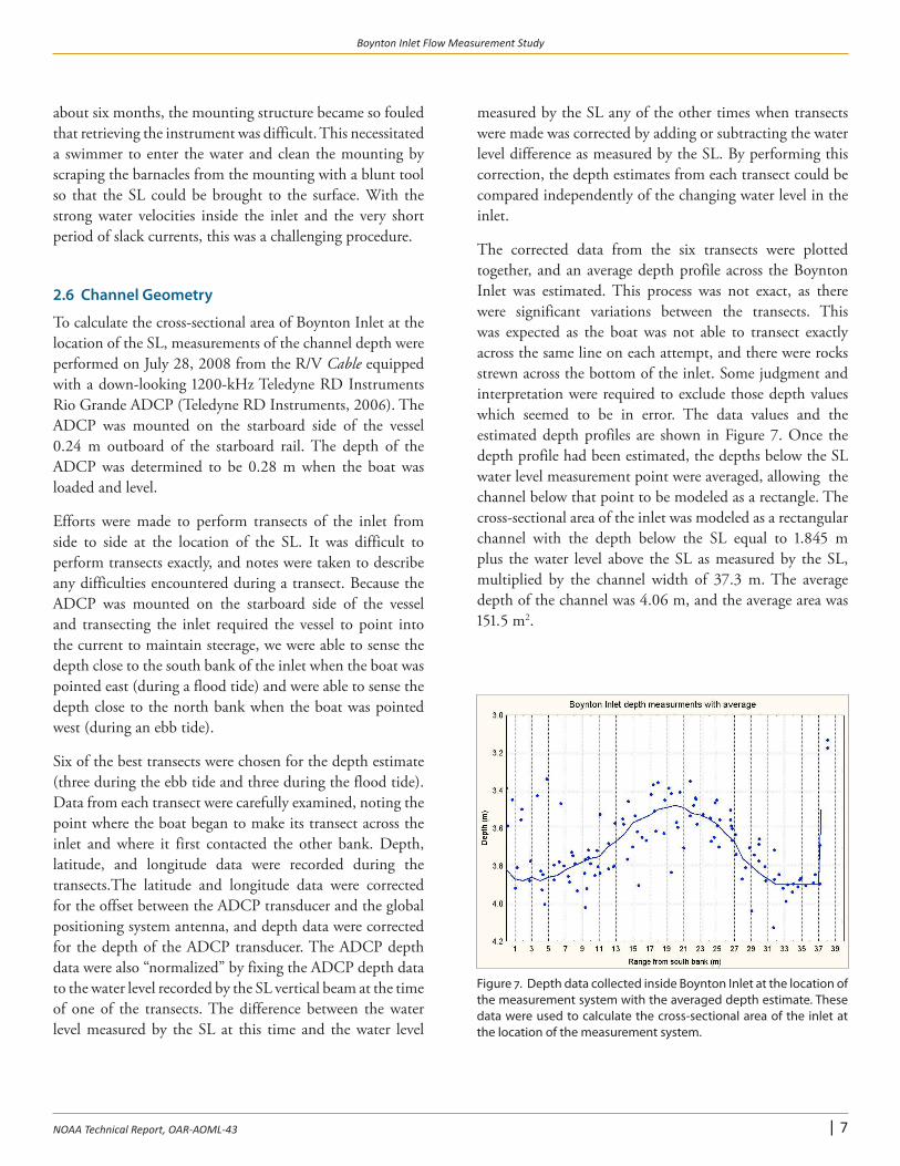
2.6 Channel Geometry

To calculate the cross‑sectional area of Boynton Inlet at the location of the SL, measurements of the channel depth were performed on July 28, 2008 from the R/V Cable equipped with a down‑looking 1200‑kHz Teledyne RD Instruments Rio Grande ADCP (Teledyne RD Instruments, 2006). The ADCP was mounted on the starboard side of the vessel 0.24 m outboard of the starboard rail. The depth of the ADCP was determined to be 0.28 m when the boat was loaded and level.

Efforts were made to perform transects of the inlet from side to side at the location of the SL. It was difficult to perform transects exactly, and notes were taken to describe any difficulties encountered during a transect. Because the ADCP was mounted on the starboard side of the vessel and transecting the inlet required the vessel to point into the current to maintain steerage, we were able to sense the depth close to the south bank of the inlet when the boat was pointed east (during a flood tide) and were able to sense the depth close to the north bank when the boat was pointed west (during an ebb tide).

Six of the best transects were chosen for the depth estimate (three during the ebb tide and three during the flood tide). Data from each transect were carefully examined, noting the point where the boat began to make its transect across the inlet and where it first contacted the other bank. Depth, latitude, and longitude data were recorded during the transects.The latitude and longitude data were corrected for the offset between the ADCP transducer and the global positioning system antenna, and depth data were corrected for the depth of the ADCP transducer. The ADCP depth data were also “normalized” by fixing the ADCP depth data to the water level recorded by the SL vertical beam at the time of one of the transects. The difference between the water level measured by the SL at this time and the water level

measured by the SL any of the other times when transects were made was corrected by adding or subtracting the water level difference as measured by the SL. By performing this correction, the depth estimates from each transect could be compared independently of the changing water level in the inlet.

The corrected data from the six transects were plotted together, and an average depth profile across the Boynton Inlet was estimated. This process was not exact, as there were significant variations between the transects. This was expected as the boat was not able to transect exactly across the same line on each attempt, and there were rocks strewn across the bottom of the inlet. Some judgment and interpretation were required to exclude those depth values which seemed to be in error. The data values and the estimated depth profiles are shown in Figure 7. Once the depth profile had been estimated, the depths below the SL water level measurement point were averaged, allowing the channel below that point to be modeled as a rectangle. The cross‑sectional area of the inlet was modeled as a rectangular channel with the depth below the SL equal to 1.845 m plus the water level above the SL as measured by the SL, multiplied by the channel width of 37.3 m. The average depth of the channel was 4.06 m, and the average area was 151.5 m2.

Figure 7. Depth data collected inside Boynton Inlet at the location of the measurement system with the averaged depth estimate. These data were used to calculate the cross-sectional area of the inlet at the location of the measurement system.

| 8



2.7 Calibration and Calculation of Index Velocity

To calculate the index velocity relationship, a set of calibration data was gathered on the flood and ebb tides and compared with the velocity measurements being made simultaneously by the fixed SL system.

2.7.1 Calibration System

To gather the calibration data, a Teledyne RD Instruments 1200‑kHz Rio Grande ADCP was mounted in an Oceanscience riverboat platform (Oceanscience, Oceanside, CA) as shown in Figure 8. The ADCP was configured to sample using a 25 cm blanking distance, a 25 cm bin size, and a sampling rate of 0.25 s. The ADCP was programmed to take one water velocity measurement ping and one bottom tracking ping during every sample. The bottom tracking ping allowed the instrument to estimate its own motion relative to the channel bottom to ensure the motion of the measurement platform did not bias the water velocity measurement. Data collected by the ADCP were transmitted via radio modem to a laptop computer which recorded and displayed the incoming data via the Teledyne RD Instruments software program WinRiver II. Clocks on the laptop computer were set to Universal Time just before each calibration exercise.

Because of the large number of vessels that transit through the Boynton Inlet during the day, it was decided to carry out the calibration exercises at night. During operations, two people were stationed on the A1A Bridge to tend the

riverboat tow line. An additional person was stationed on the bank of the inlet to guide the riverboat to the bank using a boat hook and to prevent damage to the riverboat during times when vessels transited the inlet, setting up large waves. A fourth person operated the data acquisition computer. To ensure that the riverboat operations were not a hazard to vessels navigating the channel at night, the riverboat was equipped with a flashing beacon and reflective tape. Glow sticks were attached to the riverboat tow line so that the line was visible. Personnel on the bridge and on the banks had spotlights to warn oncoming vessels of our presence and to illuminate the equipment in the water. In all cases, when an approaching vessel was sighted, the riverboat transect was aborted and the riverboat quickly brought to the edge of the inlet and illuminated by tending personnel so that our presence would be noticed by the vessel. These procedures worked very well, and no problems were encountered with vessel traffic.

For each transect, the riverboat was guided across the Boynton Inlet using a line attached to the riverboat and tended by an operator stationed on the A1A Bridge. This operator guided the riverboat from bank to bank using the tow line. At the start of the SL averaging interval (a 7.5‑minute data acquisition period occurring every 15 minutes, see sections 2.3.1 and 2.3.2), the riverboat was guided across the channel and then back, attempting to make these two crossings within the 7.5 minute SL averaging interval. It was discovered that guiding the riverboat across the channel was not a simple process. Some transects were terminated short of the total distance across the channel, and this distance was noted in the survey log. The WinRiver II software requires a user to input the starting and ending distances from the banks. These values were input during the data acquisition process and also noted in the log.

2.7.2 Calibration Data Acquisition and Processing

To gather the data necessary for the calculation of the index velocity equation, two field studies were carried out. The first study was conducted on November 7, 2007 during a flood tide and the second was conducted on January 9, 2008 during an ebb tide. During the November 2007 flood tide study, 48 transects were completed and, during the January 2008 ebb tide study, 42 transects were made. After each study, data were post processed using the WinRiver II software. A data set was constructed combining the data Figure 8. An Oceanscience riverboat system similar to the one used

to collect calibration data inside Boynton Inlet.

| 9



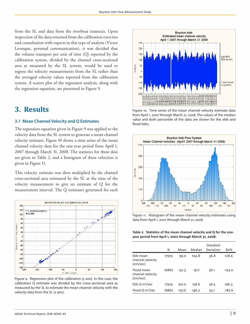
from the SL and data from the riverboat transects. Upon inspection of the data returned from the calibration exercises and consultation with experts in this type of analysis (Victor Levesque, personal communication), it was decided that the volume transport per unit of time (Q) reported by the calibration system, divided by the channel cross‑sectional area as measured by the SL system, would be used to regress the velocity measurements from the SL rather than the averaged velocity values reported from the calibration system. A scatter plot of the regression analysis, along with the regression equation, are presented in Figure 9.

3. Results3.1 Mean Channel Velocity and Q Estimates

The regression equation given in Figure 9 was applied to the velocity data from the SL system to generate a mean channel velocity estimate. Figure 10 shows a time series of the mean channel velocity data for the one‑year period from April 1, 2007 through March 31, 2008. The statistics for these data are given in Table 2, and a histogram of these velocities is given in Figure 11.

This velocity estimate was then multiplied by the channel cross‑sectional area estimated by the SL at the time of the velocity measurement to give an estimate of Q for the measurement interval. The Q estimates generated for each

Figure 9. Regression plot of the calibration (y axis). In this case, the calibration Q estimate was divided by the cross-sectional area as measured by the SL to estimate the mean channel velocity with the velocity data from the SL (x axis).

Figure 10. Time series of the mean channel velocity estimate data from April 1, 2007 through March 31, 2008. The values of the median value and 80th percentile of the data are shown for the ebb and flood tides.

Figure 11. Histogram of the mean channel velocity estimates using data from April 1, 2007 through March 31, 2008.

Table 2. Statistics of the mean channel velocity and Q for the one-year period from April 1, 2007 through March 31, 2008.

N Mean MedianStandardDeviation 80%

Ebb mean channel velocity (cm/sec)

17919 99.0 104.8 36.8 128.6

Flood mean channel velocity (cm/sec)

16862 -92.3 -97.7 36.1 -123.0

Ebb Q m3/sec 17919 150.0 158.6 56.5 196.3

Flood Q m3/sec 16862 -137.6 -146.2 53.1 -182.6

| 10



measurement interval (900 s) were then multiplied by this measurement interval to estimate the volume transport for that measurement interval. Figure 12 provides a histogram of the Q rates for the period from April 1, 2007 through March 31, 2008.

3.2 Tidal Prism Estimates

For this analysis, the start of a tidal phase (ebb or flood) was defined as that measurement in which the direction of the velocity changed sign, while the end of a tidal phase was defined as the last contiguous measurement having the same sign. The sampling interval was denoted as SI. The total volume estimates for each measurement (Q × sampling interval) contained in the interval defined in this way were summed to estimate the total volume transported through the Boynton Inlet per tidal phase (tidal prism).

ocean during the flood phase. This is consistent with the Lake Worth Lagoon receiving freshwater input from canals, precipitation, and runoff from land.

3.3 Canal Outflow and Precipitation

The per tide flow statistics presented in Table 3 indicate that there was a mean net outflow from the Boynton Inlet of approximately 470,000 m3 per tidal cycle or 3.2 × 109 m3 per year. Data from the three major canals (C51, C17, and C16) that flow into the Lake Worth Lagoon (Taylor Engineering, 2009) were compiled (Table 4). The outflow data used for this comparison were the median of the flow for the years from 1990‑2008 and the average of the flows for the years 2007‑2008. The average used as the flow for these two years was significantly less than the median of the 18‑year data (Table 4). The C51 canal flow during 2007 was the lowest of the years 1990‑2008, as was the 2005 C17 flow. However,

Figure 12. Histogram of the Q rates during flood and ebb tides for the period from April 1, 2007 through March 31, 2008.

Histograms of the tidal prisms for the interval from April 1, 2007 through March 31, 2008 are presented in Figure 13, while Table 3 presents tidal prism statistics. From Figure 13 and Table 3 it is observed that the ebb tidal phase transported more water out of the Boynton Inlet and into the ocean than was transported into the Lake Worth Lagoon from the

Figure 13. Histograms of the total volume transport per tidal phase during flood and ebb tides for the period from April 1, 2007 through March 31, 2008.

Table 3. Statistics of the tidal prism for the one-year period from April 1, 2007 through March 31, 2008.

N Mean MedianStandardDeviation 10% 90%

Ebb volumeper tide (m3 × 106)

698 3.45 3.43 0.750 2.51 4.45

Flood volumeper tide(m3 × 106)

692 2.98 3.0 0.647 2.22 3.72

∑Tide end

j=Tide startTidal prism = Qj × SI (2)

| 11



the C16 flow was 75% of the median value in 2007 and 61% of the median value in 2008. This is mentioned as the C16 canal empties into the Lake Worth Lagoon at its southern extent near the Boynton Inlet.

The mean precipitation measured at West Palm Beach International Airport for the years 1981‑2012 was 158.3 cm. The precipitation for 2007 was 161.5 cm and for 2008 it was 150.4 cm. The precipitation for the study period was not atypical.

3.4 Effects of Wind on Tidal Prism

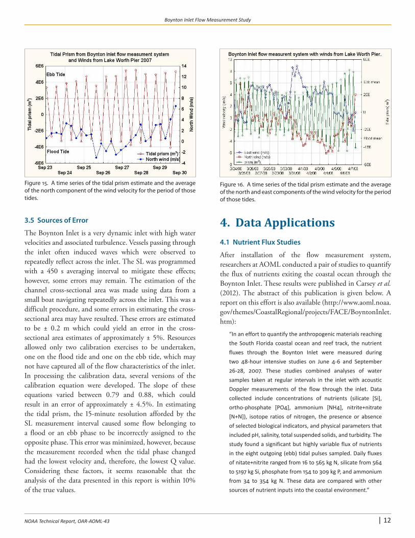
Meteorological data were gathered from the NOAA weather station LKWF1 located at the Lake Worth pier which is 7.5 km north of the Boynton Inlet and east of the Lake Worth Lagoon. The north and east components of the wind velocity were computed and averaged over the same period as the tidal volume calculations described in section 3.2. Regressions were calculated with these east and north wind velocity averages and the per tidal phase volumes (Table 5). The regressions with the east component of the wind showed weak correlations, while the regressions of the north component of the wind velocity showed stronger correlations (Figure 14). This suggests that wind from the north pushes water in the Lake Worth Lagoon to the south,

thereby increasing the ebb tide volume and suppressing the flood tide volume. Conversely, wind from the south pushes water to the north away from the Boynton Inlet, reducing the ebb tide volume and increasing the flood tide volume. Figure 15 shows an example of winds apparently affecting the flow through the inlet. On September 25, 2007, the north component of the wind for that tidal period was ‑3 m/s (wind blowing from the south). The ebb tide volume was suppressed (3.56 × 106 m3) compared to the flow volumes preceding and after this wind event. Figure 16 is another example of the tidal prism apparently being affected by winds. On March 31, 2008, a significant wind was observed with an east component of greater than 8 m/s and a north component of less than ‑4 m/s on April 1, 2008. The ebb tide prism observed on March 31, 2008 was below 1.8 × 106 m3. This value is in the lower 2% for the years of data analyzed (Table 3) and is likely a result of oceanic water and waves exerting a west‑directed pressure on the Boynton Inlet.

Table 4. Canal flow data (median of years 1990-2008 and average of years 2007-2008) and comparison with yearly (April 1, 2007- March 31, 2008) Boynton Inlet net outflow.

C51 C17 C16 Sum

Median of canal flow for years 1990-2008 (m3) 397,837,000 86,970,000 163,489,000 628,290,000

Percentage of estimated yearly inlet net outflow (321,000,000 m3)

195%

Average of canal flow for the years 2007-2008 (m3) 172,677,000 75,527,000 97,777,000 345,981,000

Percentage of estimated yearly inlet net outflow (321,000,000 m3)

108%

Table 5. Correlation (R) between north and east wind components and tidal prism.

North Wind East Wind

Ebb tide Flood tide Ebb tide Flood tide

Volumeper tide 0.37 -0.24 -0.08 Not significant

(p=0.05) Figure 14. Regression of the per tide volume transport with the north component of the wind as measured at the Lake Worth pier.

| 12



3.5 Sources of Error

The Boynton Inlet is a very dynamic inlet with high water velocities and associated turbulence. Vessels passing through the inlet often induced waves which were observed to repeatedly reflect across the inlet. The SL was programmed with a 450 s averaging interval to mitigate these effects; however, some errors may remain. The estimation of the channel cross‑sectional area was made using data from a small boat navigating repeatedly across the inlet. This was a difficult procedure, and some errors in estimating the cross‑sectional area may have resulted. These errors are estimated to be ± 0.2 m which could yield an error in the cross‑sectional area estimates of approximately ± 5%. Resources allowed only two calibration exercises to be undertaken, one on the flood tide and one on the ebb tide, which may not have captured all of the flow characteristics of the inlet. In processing the calibration data, several versions of the calibration equation were developed. The slope of these equations varied between 0.79 and 0.88, which could result in an error of approximately ± 4.5%. In estimating the tidal prism, the 15‑minute resolution afforded by the SL measurement interval caused some flow belonging to a flood or an ebb phase to be incorrectly assigned to the opposite phase. This error was minimized, however, because the measurement recorded when the tidal phase changed had the lowest velocity and, therefore, the lowest Q value. Considering these factors, it seems reasonable that the analysis of the data presented in this report is within 10% of the true values.

4. Data Applications4.1 Nutrient Flux Studies

After installation of the flow measurement system, researchers at AOML conducted a pair of studies to quantify the flux of nutrients exiting the coastal ocean through the Boynton Inlet. These results were published in Carsey et al. (2012). The abstract of this publication is given below. A report on this effort is also available (http://www.aoml.noaa.gov/themes/CoastalRegional/projects/FACE/BoyntonInlet.htm):

“In an effort to quantify the anthropogenic materials reaching the South Florida coastal ocean and reef track, the nutrient fluxes through the Boynton Inlet were measured during two 48-hour intensive studies on June 4-6 and September 26-28, 2007. These studies combined analyses of water samples taken at regular intervals in the inlet with acoustic Doppler measurements of the flow through the inlet. Data collected include concentrations of nutrients (silicate [Si], ortho-phosphate [PO4], ammonium [NH4], nitrite+nitrate [N+N]), isotope ratios of nitrogen, the presence or absence of selected biological indicators, and physical parameters that included pH, salinity, total suspended solids, and turbidity. The study found a significant but highly variable flux of nutrients in the eight outgoing (ebb) tidal pulses sampled. Daily fluxes of nitate+nitrite ranged from 16 to 565 kg N, silicate from 564 to 5197 kg Si, phosphate from 154 to 309 kg P, and ammonium from 34 to 354 kg N. These data are compared with other sources of nutrient inputs into the coastal environment.”

Figure 15. A time series of the tidal prism estimate and the average of the north component of the wind velocity for the period of those tides.

Figure 16. A time series of the tidal prism estimate and the average of the north and east components of the wind velocity for the period of those tides.

| 13



4.2 Tracers Studies and Inlet Dispersion Modeling

In an effort to study the dispersion of materials entering the coastal ocean from the Boynton Inlet on the ebb tide, a study using both Rhodamine dye and sulfur hexafluoride (SF6) as tracers was conducted in 2007. These tow tracers were injected into the inlet on an ebb tide at a known concentration. Two vessels were used to sample the tracer as it exited the inlet and dispersed into the coastal ocean. This is detailed in Carsey et al. (2013).

Data from Carsey et al. (2013) were used in an effort to model the dispersion characteristics of the Boynton Inlet, as detailed in Bloetscher et al. (2012). The abstract of this publication is provided below:

“In February 2007, a tracer study was conducted on the Boynton Inlet, Florida, using sulfur hexafluoride (SF6) tracer. The objectives of this study were to determine if the data collected from the tracer study could be used to develop a farfield model of the plume exiting the Boynton Inlet using limited data to develop a useful predictive result. There are few studies of the farfield movement of inlet plumes in the coastal ocean. The plume was successfully modeled with a Gaussian plume model that appears to mimic the response. It was noted that the tracer concentrated in a series of boluses that migrated north of the inlet. Because the project injected the tracer for only 4 hours during the outgoing tide, a long-term result that would hide the boluses was developed. The results showed velocities lower than predicted by the measured current data. The belief is that this is partially a result of tidal influences that affect outflow from the inlet.”

5. ConclusionsThe data derived from the SL flow system have been used to calculate channel velocities, flux rates, and tidal prisms for the Boynton Inlet. These measurements were examined in context with the wind stress present on the Lake Worth Lagoon and on the inlet and compared with freshwater input to the Lake Worth Lagoon through canals and by precipitation. Studies and modeling efforts using these data to examine the fate of materials exiting the Boynton Inlet into the coastal ocean were introduced and summarized. Suggestions for future work might include a similar study at the Palm Beach Inlet.

6. ReferencesAlliance for Coastal Technologies, 2005: Biofouling prevention

technologies for coastal sensors/sensor platforms. UMCES Technical Report Series TS‑426‑04‑CBL, 15 pp. (available at http://drum.lib.umd.edu/bitstream/1903/13786/1/%5BUMCES%5DCBL%2004‑016.pdf ).

Bloetscher, F., J. Pire‑Schmidt, D.E. Meeroff, T.P. Carsey, J. Stamates, K. Sullivan, and J.R. Proni, 2012: Farfield modeling of the Boynton Inlet plume. Environmental Management and Sustainable Development, 1(2):74‑89 (doi:10.5296/emsd.v1i2.2134).

Carsey, T., J. Stamates, N. Amornthammarong, J. Bishop, F. Bloetscher, C. Brown, J. Craynock, S. Cummings, P. Dammann, J. Davis, C. Featherstone, C. Fischer, K. Goodwin, D. Meeroff, J. Proni, C. Sinigalliano, P. Swart, and J.‑Z. Zhang, 2012: Boynton Inlet 48‑hour sampling intensives: June and September 2007. NOAA Technical Report, OAR‑AOML‑40, 43 pp.

Carsey, T., N. Amornthammarong, J. Bishop, F. Bloetscher, J. Craynock, S. Cummings, P. Dammann, C. Featherstone, E. Peltola, D. Pierrot, J. Proni, C. Sinigalliano, J. Stamates, K. Sullivan, and R. Wanninkhof, 2013: The Florida Outfalls and Coastal Inlets Tracer Experiment (FOCITE‑1), February 18 through March 1. NOAA Technical Report (in preparation).

Clay, C.S., and H. Medwin, 1977: Acoustical Oceanography: Principles and Applications, New York, John Wiley and Sons, 544 pp.

Florida Department of Environmental Protection, 1999: The West Palm Beach Canal, 2 pp. (available at http://www.dep.state.fl.us/southeast/ecosum/ecosums/wpbcanal.pdf ).

Levesque, V.A., and K.A. Oberg, 2012: Computing discharge using the index velocity method. U.S. Geological Survey Techniques and Methods 3‑A23, 148 pp. (available at at http://pubs.usgs.gov/tm/3a23/).

Ruhl, C.A., and M.R. Simpson, 2005: Computation of discharge using the index‑velocity method in tidally‑affected areas. U.S. Geological Survey, Scientific Investigations Report 2005‑5004, 31 pp. (available at http://pubs.usgs.gov/sir/2005/5004/sir20055004.pdf ).

SonTek Corporation, 2006: SonTek Argonaut SL system manual. San Diego, CA, 314 pp.

South Lake Worth Inlet Management Plan, 1998: Coastal Planning and Engineering, Inc., 2481 N.W. Boca Raton Boulevard, Boca Raton, FL, 33431.

Taylor Engineering, Inc., 2009: Lake Worth Lagoon watershed and stormwater loading analysis. Report submitted to the South Florida Water Management District, 186 pp.

Teledyne RD Instruments, 2006: Acoustic Doppler Current Profiler Principles of Operation: A Practical Primer, Third edition, Poway, California, 56 pp.

National Oceanic and Atmospheric AdministrationOffice of Oceanic and Atmospheric Research

Atlantic Oceanographic and Meteorological Laboratory4301 Rickenbacker Causeway

Miami, FL 33149

http://www.aoml.noaa.gov

Documents

Boynton Inlet Flow Measurement Study · Boynton Inlet Flow Measurement Study ... OAR-AOML-43 May 2013 Atlantic Oceanographic and ... and Lecia Salerno participated in the field efforts