1

Branch Flow Model: Relaxations andConvexification (Part I)

Masoud Farivar Steven H. LowEngineering and Applied Science

Caltech

Abstract—We propose a branch flow model for the anal-ysis and optimization of mesh as well as radial networks.The model leads to a new approach to solving optimalpower flow (OPF) that consists of two relaxation steps.The first step eliminates the voltage and current anglesand the second step approximates the resulting problemby a conic program that can be solved efficiently. For radialnetworks, we prove that both relaxation steps are alwaysexact, provided there are no upper bounds on loads. Formesh networks, the conic relaxation is always exact but theangle relaxation may not be exact, and we provide a simpleway to determine if a relaxed solution is globally optimal.We propose convexification of mesh networks using phaseshifters so that OPF for the convexified network can alwaysbe solved efficiently for an optimal solution. We provethat convexification requires phase shifters only outside aspanning tree of the network and their placement dependsonly on network topology, not on power flows, generation,loads, or operating constraints. Part I introduces ourbranch flow model, explains the two relaxation steps, andproves the conditions for exact relaxation. Part II describesconvexification of mesh networks, and presents simulationresults.

I. INTRODUCTION

A. Motivation

The bus injection model is the standard model forpower flow analysis and optimization. It focuses on nodalvariables such as voltages, current and power injectionsand does not directly deal with power flows on individualbranches. Instead of nodal variables, the branch flowmodel focuses on currents and powers on the branches.It has been used mainly for modeling distribution cir-cuits which tend to be radial, but has received far lessattention. In this paper, we advocate the use of branchflow model for both radial and mesh networks, anddemonstrate how it can be used for optimizing the designand operation of power systems.

Appeared in IEEE Trans. Power Systems, 28(3):2554–2564,August 2013 (submitted in May 11, 2012, accepted for publicationon March 3, 2013). A preliminary and abridged version has appearedin [1].

One of the motivations for our work is the optimalpower flow (OPF) problem. OPF seeks to optimize acertain objective function, such as power loss, gener-ation cost and/or user utilities, subject to Kirchhoff’slaws, power balance as well as capacity, stability andcontingency constraints on the voltages and power flows.There has been a great deal of research on OPF sinceCarpentier’s first formulation in 1962 [2]; surveys can befound in, e.g., [3]–[7]. OPF is generally nonconvex andNP-hard, and a large number of optimization algorithmsand relaxations have been proposed. A popular approx-imation is the DC power flow problem, which is a lin-earization and therefore easy to solve, e.g. [8]–[11]. Animportant observation was made in [12], [13] that the fullAC OPF can be formulated as a quadratically constrainedquadratic program and therefore can be approximated bya semidefinite program. While this approach is illustratedin [12], [13] on several IEEE test systems using aninterior-point method, whether or when the semidefiniterelaxation will turn out to be exact is not studied. Insteadof solving the OPF problem directly, [14] proposes tosolve its convex Lagrangian dual problem and givesa sufficient condition that must be satisfied by a dualsolution for an optimal OPF solution to be recoverable.This result is extended in [15] to include other variablesand constraints and in [16] to exploit network sparsity.In [17], [18], it is proved that the sufficient condition of[14] always holds for a radial (tree) network, providedthe bounds on the power flows satisfy a simple pattern.See also [19] for a generalization. These results confirmthat radial networks are computationally much simpler.This is important as most distribution systems are radial.

The limitation of semidefinite relaxation for OPF isstudied in [20] using mesh networks with 3, 5, and 7buses: as a line-flow constraint is tightened, the dualitygap becomes nonzero and the solutions produced by thesemidefinite relaxation becomes physically meaningless.Indeed, examples of nonconvexity have long been dis-cussed in the literature, e.g., [21]–[23]. See, e.g., [24]for branch-and-bound algorithms for solving OPF whenconvex relaxation fails.

2

The papers above are all based on the bus injectionmodel. In this paper, we introduce a branch flow modelon which OPF and its relaxations can also be defined.Our model is motivated by a model first proposed byBaran and Wu in [25], [26] for the optimal placement andsizing of switched capacitors in distribution circuits forVolt/VAR control. One of the insights we highlight hereis that the Baran-Wu model of [25], [26] can be treatedas a particular relaxation of our branch flow model wherethe phase angles of the voltages and currents are ignored.By recasting their model as a set of linear and quadraticequality constraints, [27], [28] observe that relaxing thequadratic equality constraints to inequality constraintsyields a second-order cone program (SOCP). It provesthat the SOCP relaxation is exact for radial networks,when there are no upper bounds on the loads. Thisresult is extended here to mesh networks with line limits,and convex, as opposed to linear, objective functions(Theorem 1). See also [29], [30] for various convexrelaxations of approximations of the Baran-Wu modelfor radial networks.

Other branch flow models have also been studied, e.g.,in [31]–[33], all for radial networks. Indeed [31] studiesa similar model to that in [25], [26], using receiving-end branch powers as variables instead of sending-endbranch powers as in [25], [26]. Both [32] and [33]eliminate voltage angles by defining real and imaginaryparts of V

i

V

⇤j

as new variables and defining bus powerinjections in terms of these new variables. This resultsin a system of linear quadratic equations in powerinjections and the new variables. While [32] developsa Newton-Raphson algorithm to solve the bus powerinjections, [33] solves for the branch flows through anSOCP relaxation for radial networks, though no proof ofoptimality is provided.

This set of papers [25]–[33] all exploit the fact thatpower flows can be specified by a simple set of linear andquadratic equalities if voltage angles can be eliminated.Phase angles can be relaxed only for radial networksand generally not for mesh networks, as [34] points outfor their branch flow model, because cycles in a meshnetwork impose nonconvex constraints on the optimiza-tion variables (similar to the angle recovery condition inour model; see Theorem 2 below). For mesh networks,[34] proposes a sequence of SOCP where the nononvexconstraints are replaced by their linear approximationsand demonstrates the effectiveness of this approach usingseven network examples. In this paper we extend theBaran-Wu model from radial to mesh networks and useit to develop a solution strategy for OPF.

B. Summary

Our purpose is to develop a formal theory of branchflow model for the analysis and optimization of mesh aswell as radial networks. As an illustration, we formulateOPF within this alternative model, propose relaxations,characterize when a relaxed solution is exact, prove thatour relaxations are always exact for radial networks whenthere are no upper bounds on loads but may not be exactfor mesh networks, and show how to use phase shiftersto convexify a mesh network so that a relaxed solutionis always optimal for the convexified network.

Specifically we formulate in Section II the OPF prob-lem using branch flow equations involving complex busvoltages and complex branch current and power flows.In Section III we describe our solution approach that

!"#$

!"#%&'$

!"#%('$

)*&(+$'),&*&-./$

0/1)'2)$3'.4)(-./$5.'$+'))$

/./(./1)*$

/./(./1)*$

(./1)*$

&/6,)$'),&*&-./$

(./0($'),&*&-./$

Fig. 1: Proposed solution strategy for solving OPF.

consists of two relaxation steps (see Figure 1):• Angle relaxation: relax OPF by eliminating voltage

and current angles from the branch flow equations.This yields the (extended) Baran-Wu model and arelaxed problem OPF-ar which is still nonconvexdue to a quadratic equality constraint.

• Conic relaxation: relax OPF-ar by changing thequadratic equality into an inequality constraint. Thisyields a convex problem OPF-cr (which is an SOCPwhen the objective function is linear).

In Section IV we prove that the conic relaxation OPF-cr is always exact even for mesh networks, providedthere are no upper bounds on real and reactive loads,i.e., any optimal solution of OPF-cr is also optimal forOPF-ar. Given an optimal solution of OPF-ar, whetherwe can derive an optimal solution of the original OPFdepends on whether we can recover the voltage andcurrent angles from the given OPF-ar solution. In Section

3

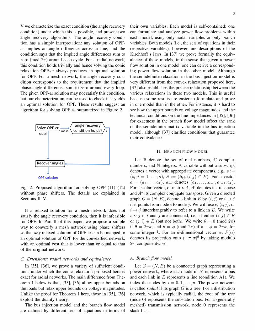
V we characterize the exact condition (the angle recoverycondition) under which this is possible, and present twoangle recovery algorithms. The angle recovery condi-tion has a simple interpretation: any solution of OPF-ar implies an angle difference across a line, and thecondition says that the implied angle differences sum tozero (mod 2⇡) around each cycle. For a radial network,this condition holds trivially and hence solving the conicrelaxation OPF-cr always produces an optimal solutionfor OPF. For a mesh network, the angle recovery con-dition corresponds to the requirement that the impliedphase angle differences sum to zero around every loop.The given OPF-ar solution may not satisfy this condition,but our characterization can be used to check if it yieldsan optimal solution for OPF. These results suggest analgorithm for solving OPF as summarized in Figure 2.

!"#$%&'()*+,&

'()&4"#7."8&

9%+"$%,&38:#%4&

,3;03#&

38:#%&,%+"$%,<&+"8;0."8&2"#;4=& >&/%42&

Fig. 2: Proposed algorithm for solving OPF (11)–(12)without phase shifters. The details are explained inSections II–V.

If a relaxed solution for a mesh network does notsatisfy the angle recovery condition, then it is infeasiblefor OPF. In Part II of this paper, we propose a simpleway to convexify a mesh network using phase shiftersso that any relaxed solution of OPF-ar can be mapped toan optimal solution of OPF for the convexified network,with an optimal cost that is lower than or equal to thatof the original network.

C. Extensions: radial networks and equivalence

In [35], [36], we prove a variety of sufficient condi-tions under which the conic relaxation proposed here isexact for radial networks. The main difference from The-orem 1 below is that, [35], [36] allow upper bounds onthe loads but relax upper bounds on voltage magnitudes.Unlike the proof for Theorem 1 here, those in [35], [36]exploit the duality theory.

The bus injection model and the branch flow modelare defined by different sets of equations in terms of

their own variables. Each model is self-contained: onecan formulate and analyze power flow problems withineach model, using only nodal variables or only branchvariables. Both models (i.e., the sets of equations in theirrespective variables), however, are descriptions of theKirchhoff’s laws. In [37] we prove formally the equiv-alence of these models, in the sense that given a powerflow solution in one model, one can derive a correspond-ing power flow solution in the other model. Althoughthe semidefinite relaxation in the bus injection model isvery different from the convex relaxation proposed here,[37] also establishes the precise relationship between thevarious relaxations in these two models. This is usefulbecause some results are easier to formulate and provein one model than in the other. For instance, it is hard tosee how the upper bounds on voltage magnitudes and thetechnical conditions on the line impedances in [35], [36]for exactness in the branch flow model affect the rankof the semidefinite matrix variable in the bus injectionmodel, although [37] clarifies conditions that guaranteetheir equivalence.

II. BRANCH FLOW MODEL

Let R denote the set of real numbers, C complexnumbers, and N integers. A variable without a subscriptdenotes a vector with appropriate components, e.g., s :=(s

i

, i = 1, . . . , n), S := (Sij

, (i, j) 2 E). For a vectora = (a1, . . . , a

k

), a�i

denotes (a1, . . . , ai�1, ai+1, ak

).For a scalar, vector, or matrix A, At denotes its transposeand A

⇤ its complex conjugate transpose. Given a directedgraph G = (N,E), denote a link in E by (i, j) or i ! j

if it points from node i to node j. We will use e, (i, j), ori ! j interchangeably to refer to a link in E. We writei ⇠ j if i and j are connected, i.e., if either (i, j) 2 E

or (j, i) 2 E (but not both). We write ✓ = 0 (mod 2⇡)if ✓ = 2⇡k, and ✓ = � (mod 2⇡) if ✓ � � = 2⇡k, forsome integer k. For an d-dimensional vector ↵, P(↵)denotes its projection onto (�⇡,⇡]d by taking modulo2⇡ componentwise.

A. Branch flow model

Let G = (N,E) be a connected graph representing apower network, where each node in N represents a busand each link in E represents a line (condition A1). Weindex the nodes by i = 0, 1, . . . , n. The power networkis called radial if its graph G is a tree. For a distributionnetwork, which is typically radial, the root of the tree(node 0) represents the substation bus. For a (generallymeshed) transmission network, node 0 represents theslack bus.

4

We regard G as a directed graph and adopt the follow-ing orientation for convenience (only). Pick any spanningtree T := (N,E

T

) of G rooted at node 0, i.e., T isconnected and E

T

✓ E has n links. All links in E

T

pointaway from the root. For any link in E \E

T

that is not inthe spanning tree T , pick an arbitrary direction. Denotea link by (i, j) or i ! j if it points from node i to nodej. Henceforth we will assume without loss of generalitythat G and T are directed graphs as described above.1 Foreach link (i, j) 2 E, let z

ij

= r

ij

+ ixij

be the compleximpedance on the line, and y

ij

:= 1/zij

=: gij

� ibij

bethe corresponding admittance. For each node i 2 N , letz

i

= r

i

+ ixi

be the shunt impedance from i to ground,and y

i

:= 1/zi

=: gi

� ibi

.2For each (i, j) 2 E, let I

ij

be the complex currentfrom buses i to j and S

ij

= P

ij

+iQij

be the sending-endcomplex power from buses i to j. For each node i 2 N ,let V

i

be the complex voltage on bus i. Let s

i

be thenet complex power injection, which is generation minusload on bus i. We use s

i

to denote both the complexnumber p

i

+ iqi

and the pair (pi

, q

i

) depending on thecontext.

As customary, we assume that the complex voltageV0 is given and the complex net generation s0 is avariable. For power flow analysis, we assume otherpower injections s := (s

i

, i = 1, . . . , n) are given. Foroptimal power flow, VAR control, or demand response,s are control variables as well.

Given z := (zij

, (i, j) 2 E, z

i

, i 2 N), V0 andbus power injections s, the variables (S, I, V, s0) :=(S

ij

, I

ij

, (i, j) 2 E, V

i

, i = 1, . . . , n, s0) satisfy theOhm’s law:

V

i

� V

j

= z

ij

I

ij

, 8(i, j) 2 E (1)

the definition of branch power flow:

S

ij

= V

i

I

⇤ij

, 8(i, j) 2 E (2)

and power balance at each bus: for all j 2 N ,X

k:j!k

S

jk

�X

i:i!j

�

S

ij

� z

ij

|Iij

|2�

+ y

⇤j

|Vj

|2 = s

j

(3)

We will refer to (1)–(3) as the branch flowmodel/equations. Recall that the cardinality |N | = n+1and let |E| =: m. The branch flow equations (1)–(3)specify 2m+ n+ 1 nonlinear equations in 2m+ n+ 1

1The orientation of G and T are different for different spanningtrees T , but we often ignore this subtlety in this paper.

2The shunt admittance yi represents capacitive devices on bus i

only and a line is modeled by a series admittance yij without shuntelements. If a shunt admittance ibij/2 is included on each end ofline (i, j) in the ⇡-model, then a limit on line flow should be a limiton

���Sij � ibij |Vi|2/2��� instead of on |Sij |.

complex variables (S, I, V, s0), when other bus powerinjections s are specified.

We will call a solution of (1)–(3) a branch flowsolution with respect to a given s, and denote it byx(s) := (S, I, V, s0). Let X(s) ✓ C2m+n+1 be the setof all branch flow solutions with respect to a given s:

X(s) := {x := (S, I, V, s0) |x solves (1)–(3) given s}(4)

and let X be the set of all branch flow solutions:

X :=[

s2Cn

X(s) (5)

For simplicity of exposition, we will often abuse notationand use X to denote either the set defined in (4) orthat in (5), depending on the context. For instance, Xis used to denote the set in (4) for a fixed s in Section Vfor power flow analysis, and to denote the set in (5) inSection IV for optimal power flow where s itself is alsoan optimization variable. Similarly for other variablessuch as x for x(s).

B. Optimal power flow

Consider the optimal power flow problem where,in addition to (S, I, V, s0), s is also an optimizationvariable. Let p

i

:= p

g

i

� p

c

i

and q

i

:= q

g

i

� q

c

i

where p

g

i

and q

g

i

(pci

and q

c

i

) are the real and reactive power gen-eration (consumption) at node i. For instance, [25], [26]formulate a Volt/VAR control problem for a distributioncircuit where q

g

i

represent the placement and sizing ofshunt capacitors. In addition to (1)–(3), we impose thefollowing constraints on power generation: for i 2 N ,

p

g

i

p

g

i

p

g

i

, q

g

i

q

g

i

q

g

i

(6)

In particular, any of p

g

i

, q

g

i

can be a fixed constant byspecifying that pg

i

= p

g

i

and/or qgi

= q

g

i

. For instance, inthe inverter-based VAR control problem of [27], [28], pg

i

are the fixed (solar) power outputs and the reactive powerq

g

i

are the control variables. For power consumption, werequire, for i 2 N ,

p

c

i

p

c

i

p

c

i

, q

c

i

q

c

i

q

c

i

(7)

The voltage magnitudes must be maintained in tightranges: for i = 1, . . . , n,

v

i

|Vi

|2 v

i

(8)

Finally, we impose flow limits in terms of branch cur-rents: for all (i, j) 2 E,

|Iij

| I

ij

(9)

5

We allow any objective function that is convex anddoes not depend on the angles \V

i

,\Iij

of voltages andcurrents. For instance, suppose we aim to minimize realpower losses r

ij

|Iij

|2 [38], [39], minimize real powergeneration costs c

i

p

g

i

, and maximize energy savingsthrough conservation voltage reduction (CVR). Then theobjective function takes the form (see [27], [28])

X

(i,j)2E

r

ij

|Iij

|2 +X

i2Nc

i

p

g

i

+X

i2N↵

i

|Vi

|2 (10)

for some given constants c

i

,↵

i

� 0.To simplify notation, let `

ij

:= |Iij

|2 and v

i

:= |Vi

|2.Let sg := (sg

i

, i = 1, . . . , n) = (pgi

, q

g

i

, i = 1, . . . , n) bethe power generations, and s

c := (sci

, i = 1, . . . , n) =(pc

i

, q

c

i

, i = 1, . . . , n) the power consumptions. Let s

denote either sg�s

c or (sg, sc) depending on the context.Given a branch flow solution x := x(s) := (S, I, V, s0)with respect to a given s, let y := y(s) := (S, `, v, s0) de-note the projection of x that have phase angles \V

i

,\Iij

eliminated. This defines a projection function h such thaty = h(x), to which we will return in Section III. Thenour objective function is f

⇣

h(x), s⌘

. We assume f (y, s)

is convex (condition A2); in addition, we assume f isstrictly increasing in `

ij

, (i, j) 2 E, nonincreasing inload s

c, and independent of S (condition A3). Let

S := { (S, v, s0, s) | (v, s0, s) satisfies (6)� (9) }

All quantities are optimization variables, except V0

which is given.The optimal power flow problem is

OPF:

minx,s

f

⇣

h(x), s⌘

(11)

subject to x 2 X, (S, v, s0, s) 2 S (12)

where X is defined in (5).The feasible set is specified by the nonlinear branch

flow equations and hence OPF (11)–(12) is in generalnonconvex and hard to solve. The goal of this paper isto propose an efficient way to solve OPF by exploitingthe structure of the branch flow model.

C. Notations and assumptions

The main variables and assumptions are summarizedin Table I and below for ease of reference:A1 The network graph G is connected.A2 The cost function f(y, s) for optimal power flow is

convex.A3 The cost function f(y, s) is strictly increasing in `,

nonincreasing in load s

c, and independent of S.A4 The optimal power flow problem OPF (11)–(12) is

feasible.

TABLE I: Notations.

G, T (directed) network graph G and a span-ning tree T of G

B, BT reduced (and transposed) incidencematrix of G and the submatrix corre-sponding to T

Vi, vi complex voltage on bus i with vi :=|Vi|2

si = pi + iqi net complex load power on bus i

pi = p

gi � p

ci net real power equals generation minus

load;qi = q

gi � q

ci net reactive power equals generation

minus loadIij , `ij complex current from buses i to j with

`ij := |Iij |2Sij = Pij + iQij complex power from buses i to j

(sending-end)X set of all branch flow solutions that

satisfy (1)–(3) either for some s, orfor a given s (sometimes denoted moreaccurately by X(s));

Y set of all relaxed branch flow solutionsthat satisfy (13)–(16) either for a givens or for some s;

Y set of all relaxed branch flow solutionsthat satisfy (13)–(15) and (22) eitherfor a given s or for some s;

x = (S, I, V, s0) 2 X vector x of power flow variablesy = (S, `, v, s0) 2 Y and its projection y;y = h(x); x = h✓(y) projection mapping y and an inverse h✓

zij , yi impedance on line (i, j) and shunt ad-mittance from bus i to ground

f = f

⇣h(x), s

⌘objective function of OPF

These assumptions are standard and realistic. For in-stance, the objective function in (10) satisfies conditionsA2–A3. A3 is a property of the objective function f andnot a property of power flow solutions; it holds if thecost function is strictly increasing in line loss.

III. RELAXATIONS AND SOLUTION STRATEGY

A. Relaxed branch flow model

Substituting (2) into (1) yields V

j

= V

i

� z

ij

S

⇤ij

/V

⇤i

.Taking the magnitude squared, we have v

j

= v

i

+|z

ij

|2`ij

� (zij

S

⇤ij

+ z

⇤ij

S

ij

). Using (3) and (2) and interms of real variables, we therefore have

p

j

=X

k:j!k

P

jk

�X

i:i!j

(Pij

� r

ij

`

ij

) + g

j

v

j

, 8j (13)

q

j

=X

k:j!k

Q

jk

�X

i:i!j

(Qij

� x

ij

`

ij

) + b

j

v

j

, 8j(14)

v

j

= v

i

� 2(rij

P

ij

+ x

ij

Q

ij

) + (r2ij

+ x

2ij

)`ij

8(i, j) 2 E (15)

`

ij

=P

2ij

+Q

2ij

v

i

, 8(i, j) 2 E (16)

6

We will refer to (13)–(16) as the relaxed (branchflow) model/equations and a solution a relaxed (branchflow) solution. These equations were first proposedin [25], [26] to model radial distribution circuits.They define a system of equations in the variables(P,Q, `, v, p0, q0) := (P

ij

, Q

ij

, `

ij

, (i, j) 2 E, v

i

, i =1, . . . , n, p0, q0). We often use (S, `, v, s0) as a short-hand for (P,Q, `, v, p0, q0). The relaxed model has asolution under A4.

In contrast to the original branch flow equations (1)–(3), the relaxed equations (13)–(16) specifies 2(m+n+1)equations in 3m+n+2 real variables (P,Q, `, v, p0, q0),given s. For a radial network, i.e., G is a tree, m =|E| = |N | � 1 = n. Hence the relaxed system (13)–(16) specifies 4n+ 2 equations in 4n+ 2 real variables.It is shown in [40] that there are generally multiplesolutions, but for practical networks where |V0| ' 1 andr

ij

, x

ij

are small p.u., the solution of (13)–(16) is unique.Exploiting structural properties of the Jacobian matrix,efficient algorithms have also been proposed in [41] tosolve the relaxed branch flow equations.

For a connected mesh network, m = |E| > |N |�1 =n, in which case there are more variables than equationsfor the relaxed model (13)–(16), and therefore the so-lution is generally nonunique. Moreover, some of thesesolutions may be spurious, i.e., they do not correspond toa solution of the original branch flow equations (1)–(3).

Indeed, one may consider (S, `, v, s0) as a projectionof (S, I, V, s0) where each variable I

ij

or V

i

is relaxedfrom a point in the complex plane to a circle with aradius equal to the distance of the point from the origin.It is therefore not surprising that a relaxed solution of(13)–(16) may not correspond to any solution of (1)–(3). The key is whether, given a relaxed solution, wecan recover the angles \V

i

,\Iij

correctly from it. Itis then remarkable that, when G is a tree, indeed thesolutions of (13)–(16) coincide with those of (1)–(3).Moreover for a general network, (13)–(16) together withthe angle recovery condition in Theorem 2 below areindeed equivalent to (1)–(3), as explained in Remark 5of Section V.

To understand the relationship between the branchflow model and the relaxed model and formulate ourrelaxations precisely, we need some notations. Fix ans. Given a vector (S, I, V, s0) 2 C2m+n+1, define itsprojection h : C2m+n+1 ! R3m+n+2 by h(S, I, V, s0) =(P,Q, `, v, p0, q0) where

P

ij

= Re S

ij

, Q

ij

= Im S

ij

, `

ij

= |Iij

|2 (17)p

i

= Re s

i

, q

i

= Im s

i

, v

i

= |Vi

|2 (18)

Let Y ✓ C2m+n+1 denote the set of all y := (S, I, V, s0)

h

h!

C2m+n+1 R3m+n+2

YY

X h X( )

Fig. 3: X is the set of branch flow solutions andY = h(Y) is the set of relaxed solutions. The inverseprojection h

✓

is defined in Section V.

whose projections are the relaxed solutions:3

Y :=n

y := (S, I, V, s0)|h(y) solves (13)–(16)o

(19)

Define the projection Y := h(Y) of Y onto the spaceR2m+n+1 as

Y := { y := (S, `, v, s0) | y solves (13)–(16) }

Clearly

X ✓ Y and h(X) ✓ h(Y) =: Y

Their relationship is illustrated in Figure 3.

B. Two relaxations

Consider the OPF with angles relaxed:

minx,s

f

⇣

h(x), s⌘

subject to x 2 Y, (S, v, s0, s) 2 S

Clearly, this problem provides a lower bound to theoriginal OPF problem since Y ◆ X. Since neither h(x)nor the constraints in Y involves angles \V

i

,\Iij

, thisproblem is equivalent to the followingOPF-ar:

miny,s

f (y, s) (20)

subject to y 2 Y, (S, v, s0, s) 2 S (21)

The feasible set of OPF-ar is still nonconvex due to thequadratic equalities in (16). Relax them to inequalities:

`

ij

�P

2ij

+Q

2ij

v

i

, (i, j) 2 E (22)

3As mentioned earlier, the set defined in (19) is strictly speakingY(s) with respect to a fixed s. To simplify exposition, we abusenotation and use Y to denote both Y(s) and

Ss2Cn Y(s), depending

on the context. The same applies to Y and Y etc.

7

Define the convex second-order cone (see Theorem 1below) Y ✓ R2m+n+1 that contains Y as

Y := {y := (S, `, v, s0) | y solves (13)–(15) and (22)}

Consider the following conic relaxation of OPF-ar:OPF-cr:

miny,s

f (y, s) (23)

subject to y 2 Y, (S, v, s0, s) 2 S (24)

Clearly OPF-cr provides a lower bound to OPF-ar sinceY ◆ Y.

C. Solution strategy

In the rest of this paper, we will prove the following:1) OFP-cr is convex. Moreover, if there are no upper

bounds on loads, then the conic relaxation is exactso that any optimal solution (y

cr

, s

cr

) of OPF-cris also optimal for OPF-ar for mesh as well asradial networks (Section IV, Theorem 1). OPF-cris a SOCP when the objective function is linear.

2) Given a solution (yar

, s

ar

) of OPF-ar, if the networkis radial, then we can always recover the phaseangles \V

i

,\Iij

uniquely to obtain an optimalsolution (x⇤, s⇤) of the original OPF through aninverse projection (Section V, Theorems 2 and 4).

3) For a mesh network, an inverse projection maynot exist to map the given (y

ar

, s

ar

) to a feasiblesolution of OPF. Our characterization can be usedto determined if (y

ar

, s

ar

) is globally optimal.These results motivate the algorithm in Figure 2.

In Part II of this paper, we show that a mesh networkcan be convexified so that (y

ar

, s

ar

) can always bemapped to an optimal solution of OPF for the convex-ified network. Moreover, convexification requires phaseshifters only on lines outside an arbitrary spanning treeof the network graph.

IV. EXACT CONIC RELAXATION

Our first key result says that OPF-cr is exact and aSOCP when the objective function is linear.

Theorem 1: Suppose p

c

i

= q

c

i

= 1, i 2 N . ThenOPF-cr is convex. Moreover, it is exact, i.e., any optimalsolution of OPF-cr is also optimal for OPF-ar.

Proof: The feasible set is convex since the nonlinearinequalities in Y can be written as the following secondorder cone constraint:

�

�

�

�

�

�

2Pij

2Qij

`

ij

� v

i

�

�

�

�

�

�

2

`

ij

+ v

i

Since the objective function is convex, OPF-cr is a conicoptimization.4 To prove that the relaxation is exact, itsuffices to show that any optimal solution of OPF-crattains equality in (22).

Assume for the sake of contradiction that (y⇤, s⇤) :=(S⇤, `⇤, v⇤, s

g

⇤0, sc

⇤0, sg

⇤, sc

⇤) is optimal for OPF-cr, but alink (i, j) 2 E has strict inequality, i.e., [v⇤]i[`⇤]ij >

[P⇤]ij2+[Q⇤]ij

2. For some " > 0 to be determined below,consider another point (y, s) = (S, ˜, v, sg0, s

c

0, sg

, s

c)defined by:

v = v⇤, s

g = s

g

⇤˜ij

= [`⇤]ij � ",

˜�ij

= [`⇤]�ij

S

ij

= [S⇤]ij � z

ij

"/2, S�ij

= [S⇤]�ij

s

c

i

= [sc⇤]i + z

ij

"/2, s

c

j

= [sc⇤]j + z

ij

"/2s

c

�i

= [sc⇤]�i

, s

c

�j

= [sc⇤]�j

where a negative index means excluding the indexedelement from a vector. Since ˜

ij

= [`⇤]ij � ", (y, s) hasa strictly smaller objective value than (y⇤, s⇤) becauseof assumption A3. If (y, s) is a feasible point, then itcontradicts the optimality of (y⇤, s⇤).

It suffices then to check that there exists an " > 0such that (y, s) satisfies (6)–(9), (13)–(15) and (22), andhence is indeed a feasible point. Since (y⇤, s⇤) is feasible,(6)–(9) hold for (y, s) too. Similarly, (y, s) satisfies (13)–(14) at all nodes k 6= i, j and (15), (22) over all links(k, l) 6= (i, j). We now show that (y, s) satisfies (13)–(14) also at nodes i, j, and (15), (22) over (i, j).

Proving (13)–(14) is equivalent to proving (3). At nodei, we have

s

i

= s

g

i

� s

c

i

= [sg⇤]i � [sc⇤]i � z

ij

"/2

=X

i!j

0

[S⇤]ij0 �X

k!i

([S⇤]ki

� z

ki

[`⇤]ki

)

+y

⇤i

v

i

� z

ij

"/2

=X

i!j

0,j

0 6=j

S

ij

0 +⇣

S

ij

+ z

ij

"/2⌘

�X

k!i

⇣

S

ki

� z

ki

˜ki

⌘

+ y

⇤i

v

i

� z

ij

"/2

=X

i!j

0

S

ij

0 �X

k!i

⇣

S

ki

� z

ki

˜ki

⌘

+ y

⇤i

v

i

4The case of linear objective without line limits is proved in [27]for radial networks. This result is extended here to mesh networkswith line limits and convex objective functions.

8

At node j, we have

s

j

= s

g

j

� s

c

j

= [sg⇤]j � [sc⇤]j � z

ij

"/2

=X

j!k

[S⇤]jk

�X

i

0!j

([S⇤]i0j � z

i

0j

[`⇤]i0j)

+y

⇤j

v

j

� z

ij

"/2

=X

j!k

S

jk

�X

i

0!j,i

0 6=i

⇣

S

i

0j

� z

i

0j

˜i

0j

⌘

+ y

⇤j

v

j

�⇣

(Sij

+ z

ij

"/2)� z

ij

(˜ij

+ ")⌘

� z

ij

"/2

=X

j!k

S

jk

�X

i

0!j

⇣

S

i

0j

� z

i

0j

˜i

0j

⌘

+ y

⇤j

v

j

Hence (13)–(14) hold at nodes i, j.For (15) across link (i, j):

v

j

= [v⇤]i � 2(rij

[P⇤]ij + x

ij

[Q⇤]ij)

+(r2ij

+ x

2ij

)[`⇤]ij

= v

i

� 2(rij

P

ij

+ x

ij

Q

ij

) + (r2ij

+ x

2ij

)˜ij

For (22) across link (i, j), we have

v

i

˜ij

� P

2ij

� Q

2ij

= [v⇤]i ([`⇤]ij � ")� ([P⇤]ij � r

ij

"/2)2

� ([Q⇤]ij � x

ij

"/2)2

=�

[v⇤]i[`⇤]ij � [P⇤]2ij

� [Q⇤]2ij

�

�" ([v⇤]i � r

ij

[P⇤]ij � x

ij

[Q⇤]ij

+ "(r2ij

+ x

2ij

)/4�

Since [v⇤]i[`⇤]ij � [P⇤]2ij

� [Q⇤]2ij

> 0, we can choose an" > 0 sufficiently small such that ˜

ij

� (P 2ij

+ Q

2ij

)/vi

.This completes the proof.Remark 1: Assumption A3 is used in the proof here

to contradict the optimality of (y⇤, s⇤). Instead of A3, iff(y, s) is nondecreasing in `, the same argument showsthat, given an optimal (y⇤, s⇤) with a strict inequality[v⇤]i[`⇤]ij > [P⇤]ij

2 + [Q⇤]ij2, one can choose " > 0 to

obtain another optimal point (y, s) that attains equalityand has a cost f(y, s) f(y⇤, s⇤). Without A3, there isalways an optimal solution of OPF-cr that is also optimalfor OPF-ar, even though it is possible that the convexrelaxation OPF-cr may also have other optimal pointswith strict inequality that are infeasible for OPF-ar.

Remark 2: The condition in Theorem 1 is equivalentto the “over-satisfaction of load” condition in [14], [17].It is needed because we have increased the loads s

c

⇤ onbuses i and j to obtain the alternative feasible solution(y, s). As we show in the simulations in [42], it issufficient but not necessary. See also [35], [36] for exactconic relaxation of OPF-cr for radial networks where thiscondition is replaced by other assumptions.

V. ANGLE RELAXATION

Theorem 1 justifies solving the convex problem OPF-cr for an optimal solution of OPF-ar. Given a solution(y, s) of OPF-ar, when and how can we recover asolution (x, s) of the original OPF (11)–(12)? It dependson whether we can recover a solution x to the branchflow equations (1)–(3) from y, given any s.

Hence, for the rest of Section V, we fix an s. We abusenotation in this section and write x, y, ✓,X,Y, Y insteadof x(s), y(s), ✓(s),X(s),Y(s), Y(s) respectively.

A. Angle recovery condition

Fix a relaxed solution y := (S, `, v, s0) 2 Y. Definethe (n+ 1)⇥m incidence matrix C of G by

C

ie

=

8

>

<

>

:

1 if link e leaves node i

�1 if link e enters node i

0 otherwise(25)

The first row of C corresponds to node 0 where V0 =|V0|ei✓0 is given. In this paper we will only work withthe m ⇥ n reduced incidence matrix B obtained fromC by removing the first row (corresponding to V0) andtaking the transpose, i.e., for e 2 E, i = 1, . . . , n,

B

ei

=

8

>

<

>

:

1 if link e leaves node i

�1 if link e enters node i

0 otherwise,

Since G is connected, m � n and rank(B) = n [43].Fix any spanning tree T = (N,E

T

) of G. We canassume without loss of generality (possibly after re-labeling some of the links) that E

T

consists of linkse = 1, . . . , n. Then B can be partitioned into

B =

B

T

B?

�

(26)

where the n⇥n submatrix B

T

corresponds to links in T

and the (m�n)⇥n submatrix B? corresponds to linksin T

? := G \ T .Let � := �(y) 2 (�⇡,⇡]m be defined by:

�

ij

:= \�

v

i

� z

⇤ij

S

ij

�

, (i, j) 2 E (27)

Informally, �ij

is the phase angle difference across link(i, j) that is implied by the relaxed solution y. Write �

as

� =

�

T

�?

�

(28)

where �

T

is n⇥ 1 and �? is (m� n)⇥ 1.Recall the projection mapping h : C2m+n+1 !

R3m+n+2 defined in (17)–(18). For each ✓ := (✓i

, i =1, . . . , n) 2 (�⇡,⇡]n, define the inverse projection

9

h

✓

: R3m+n+2 ! C2m+n+1 by h

✓

(P,Q, `, v, p0, q0) =(S, I, V, s0) where

S

ij

:= P

ij

+ iQij

(29)I

ij

:=p

`

ij

e

i(✓i�\Sij) (30)V

i

:=pv

i

e

i✓i (31)s0 := p0 + iq0 (32)

These mappings are illustrated in Figure 3.By definition of h(X) and Y, a branch flow solution

in X can be recovered from a given relaxed solution y

if y is in h(X) and cannot if y is in Y \ h(X). In otherwords, h(X) consists of exactly those points y 2 Y forwhich there exist ✓ such that their inverse projectionsh

✓

(y) are in X. Our next key result characterizes theexact condition under which such an inverse projectionexists, and provides an explicit expression for recoveringthe phase angles \V

i

,\Iij

from the given y.A cycle c in G is an ordered list c = (i1, . . . , i

k

) ofnodes in N such that (i1 ⇠ i2), . . . , (i

k

⇠ i1) are alllinks in E. We will use ‘(i, j) 2 c’ to denote a linki ⇠ j in the cycle c. Each link i ⇠ j may be in the sameorientation ((i, j) 2 E) or in the opposite orientation((j, i) 2 E). Let � be the extension of � from directedlinks to undirected links: if (i, j) 2 E then �

ij

:= �

ij

and�

ji

:= ��

ij

. For any d-dimensional vector ↵, let P(↵)denote its projection onto (�⇡,⇡]d by taking modulo 2⇡componentwise.

Theorem 2: Let T be any spanning tree of G. Con-sider a relaxed solution y 2 Y and the corresponding� = �(y) defined in (27)–(28).

1) There exists a unique ✓⇤ 2 (�⇡,⇡]n such thath

✓⇤(y) is a branch flow solution in X if and only if

B?B�1T

�

T

= �? (mod 2⇡) (33)

2) The angle recovery condition (33) holds if and onlyif for every cycle c in G

X

(i,j)2c

�

ij

= 0 (mod 2⇡) (34)

3) If (33) holds then ✓⇤ = P�

B

�1T

�

T

�

.Remark 3: Given a relaxed solution y, Theorem 2

prescribes a way to check if a branch flow solution canbe recovered from it, and if so, the required computation.The angle recovery condition (33) depends only onthe network topology through the reduced incidencematrix B. The choice of spanning tree T correspondsto choosing n linearly independent rows of B to formB

T

and does not affect the conclusion of the theorem.Remark 4: When it holds, the angle recovery condi-

tion (34) has a familiar interpretation (due to Lemma 3

below): the voltage angle differences (implied by y) sumto zero (mod 2⇡) around any cycle.

Remark 5: A direct consequence of Theorem 2 is thatthe relaxed branch flow model (13)–(16) together withthe angle recovery condition (33) is equivalent to theoriginal branch flow model (1)–(3). That is, x satisfies(1)–(3) if and only if y = h(x) satisfies (13)–(16) and(33). The challenge in computing a branch flow solutionx is that (33) is nonconvex.

The proof of Theorem 2 relies on the followingimportant lemma that gives a necessary and sufficientcondition for an inverse projection h

✓

(y) defined by(29)–(32) to be a branch flow solution in X. Fix anyy := (S, `, v, s0) in Y and the corresponding � := �(y)defined in (27). Consider the equation

B✓ = � + 2⇡k (35)

where k 2 Nm is an integer vector. Since G is connected,m � n and rank(B) = n. Hence, given any k, there isat most one ✓ that solves (35). Obviously, given any ✓,there is exactly one k that solves (35); we denote it byk(✓) when we want to emphasize the dependence on ✓.Given any solution (✓, k) with ✓ 2 (�⇡,⇡]n, define itsequivalence class by 5

�(✓, k) := {(✓ + 2⇡↵, k +B↵) | ↵ 2 Nn}

We say �(✓, k) is a solution of (35) if every vector in�(✓, k) is a solution of (35), and �(✓, k) is the uniquesolution of (35) if it is the only equivalence class ofsolutions.

Lemma 3: Given any y := (S, `, v, s0) in Y and thecorresponding � := �(y) defined in (27):

1) h

✓

(y) is a branch flow solution in X if and only if(✓, k(✓)) solves (35).

2) there is at most one �(✓, k), ✓ 2 (�⇡,⇡]n, that isthe unique solution of (35), when it exists.Proof: Suppose (✓, k) is a solution of (35) for some

k = k(✓). We need to show that (13)–(16) together with(29)–(32) and (35) imply (1)–(3). Now (13) and (14) areequivalent to (3). Moreover (16) and (29)–(31) imply (2).To prove (1), substitute (2) into (35) to get

✓

i

� ✓

j

= \�

v

i

� z

⇤ij

V

i

I

⇤ij

�

+ 2⇡kij

= \ V

i

(Vi

� z

ij

I

ij

)⇤ + 2⇡kij

Hence

\Vj

= ✓

j

= \ (Vi

� z

ij

I

ij

)� 2⇡kij

(36)

5Using the connectedness of G and the definition of B, one canargue that ↵ must be an integer vector for k +B↵ to be integral.

10

From (15) and (2), we have

|Vj

|2 = |Vi

|2 + |zij

|2|Iij

|2 � (zij

S

⇤ij

+ z

⇤ij

S

ij

)

= |Vi

|2 + |zij

|2|Iij

|2 � (zij

V

⇤i

I

ij

+ z

⇤ij

V

i

I

⇤ij

)

= |Vi

� z

ij

I

ij

|2

This and (36) imply V

j

= V

i

� z

ij

I

ij

which is (1).Conversely, suppose h

✓

(y) 2 X. From (1) and (2), wehave V

i

V

⇤j

= |Vi

|2 � z

⇤ij

S

ij

. Then ✓

i

� ✓

j

= �

ij

+ 2⇡kij

for some integer kij

= k

ij

(✓). Hence (✓, k) solves (35).The discussion preceding the lemma shows that, given

any k 2 Nm, there is at most one ✓ that satisfies (35).If no such ✓ exists for any k 2 Nm, then (35) hasno solution (✓, k). If (35) has a solution (✓, k), thenclearly (✓ + 2⇡↵, k + B↵) are also solutions for all↵ 2 Nn. Hence we can assume without loss of generalitythat ✓ 2 (�⇡,⇡]n. We claim that �(✓, k) is the uniquesolution of (35). Otherwise, there is an (✓, k) 62 �(✓, k)with B✓ = � + 2⇡k. Then B(✓ � ✓) = 2⇡(k � k),or k = k + B↵ for some ↵. Since k 2 Nm, ↵ is aninteger vector; moreover ✓ is unique given k. This means(✓, k) 2 �(✓, k), a contradiction.

Proof of Theorem 2: Since m � n and rank(B) =n, we can always find n linearly independent rows ofB to form a basis. The choice of this basis correspondsto choosing a spanning tree of G, which always existssince G is connected [44, Chapter 5]. Assume withoutloss of generality that the first n rows is such a basisso that B and � are partitioned as in (26) and (28)respectively. Then Lemma 3 implies that h

✓⇤(y) 2 Xwith ✓⇤ 2 (�⇡,⇡]n if and only if (✓⇤, k⇤(✓⇤)) is theunique solution of

B

T

B?

�

✓ =

�

T

�?

�

+ 2⇡

k

T

k?

�

(37)

Since T is a spanning tree, the n ⇥ n submatrix B

T

is invertible. Moreover (37) has a unique solution ifand only if B?B

�1T

(�T

+ 2⇡kT

) = �? + 2⇡k?, i.e.,B?B

�1T

�

T

= �?+2⇡k? where k? := k?�B?B�1T

k

T

.Then (38) below implies that k? is an integer vector.This proves the first assertion.

For the second assertion, recall that the spanning treeT defines the orientation of all links in T to be directedaway from the root node 0. Let T (i ; j) denote theunique path from node i to node j in T ; in particular,T (0 ; j) consists of links all with the same orientationas the path and T (j ; 0) of links all with the oppositeorientation. Then it can be verified directly that

⇥

B

�1T

⇤

ei

:=

(

�1 if link e is in T (0 ; i)

0 otherwise(38)

Hence B

�1T

�

T

represents the (negative of the) sum ofangle differences on the path T (0 ; i) for each nodei 2 T :⇥

B

�1T

�

T

⇤

i

=X

e

⇥

B

�1T

⇤

ie

[�T

]e

= �X

e2T (0;i)

[�T

]e

Hence B?B�1T

�

T

is the sum of voltage angle differencesfrom node i to node j along the unique path in T , forevery link (i, j) 2 E \E

T

not in the tree T . To see this,we have, for each link e := (i, j) 2 E \ E

T

,⇥

B?B�1T

�

T

⇤

e

=⇥

B

�1T

�

T

⇤

i

�⇥

B

�1T

�

T

⇤

j

=X

e

02T (0;j)

[�T

]e

0 �X

e

02T (0;i)

[�T

]e

0

SinceX

e

02T (0;j)

[�T

]e

0 = �X

e

02T (j;0)

h

�

T

i

e

0

the angle recovery condition (33) is equivalent toX

e

02T (0;i)

[�T

]e

0 + [�?]ij

+X

e

02T (j;0)

h

�

T

i

e

0

=X

e

02c(i,j)

�

e

0 = 0 (mod 2⇡)

where c(i, j) denotes the unique basis cycle (with respectto T ) associated with each link (i, j) not in T [44,Chapter 5]. Hence (33) is equivalent to (34) on all basiscycles, and therefore it is equivalent to (34) on all cycles.

Suppose (33) holds and let (✓⇤, k⇤) be the unique solu-tion of (37) with ✓⇤ 2 (�⇡,⇡]n. We are left to show that✓⇤ = P

�

B

�1T

�

T

�

. By (37) we have ✓⇤ � 2⇡B�1T

[k⇤]T =�

T

. Consider ↵ := �B

�1T

[k⇤]T which is in Nn dueto (38). Then (✓⇤ + 2⇡↵, k⇤ + B↵) 2 �(✓⇤, k⇤) andhence is also a solution of (37) by Lemma 3. Moreover✓⇤+2⇡↵ = B

�1T

�

T

since [k⇤]T +B

T

↵ = 0. This meansthat ✓⇤ is given by P

�

B

�1T

�

T

�

since ✓⇤ 2 (�⇡,⇡]n.

B. Angle recovery algorithms

Theorem 2 suggests a centralized method to computea branch flow solution from a relaxed solution.Algorithm 1: centralized angle recovery. Given arelaxed solution y 2 Y,

1) Choose any n basis rows of B and form B

T

, B?.2) Compute � from y and check if B?B

�1T

�

T

��? =0 (mod 2⇡).

3) If not, then y 62 h(X); stop.4) Otherwise, compute ✓⇤ = P

�

B

�1T

�

T

�

.5) Compute h

✓⇤(y) 2 X through (29)–(32).Theorem 2 guarantees that h

✓⇤(y), if exists, is the uniquebranch flow solution of (1)–(3) whose projection is y.

11

The relations (2) and (35) motivate an alternativeprocedure to compute the angles \I

ij

, \Vi

, and a branchflow solution. This procedure is more amenable to adistributed implementation.Algorithm 2: distributed angle recovery. Given arelaxed solution y 2 Y,

1) Choose any spanning tree T of G rooted at node 0.2) For j = 0, 1, . . . , n (i.e., as j ranges over the tree T ,

starting from the root and in the order of breadth-first search), for all children k with j ! k, set

\Ijk

:= \Vj

� \Sjk

(39)\V

k

:= \Vj

� \(vj

� z

⇤jk

S

jk

) (40)

3) For each link (j, k) 2 E \ ET

not in the spanningtree, node j is an additional parent of k in additionto k’s parent in the spanning tree from which \V

k

has already been computed in Step 2.a) Compute current angle \I

jk

using (39).b) Compute a new voltage angle ✓

j

k

using the newparent j and (40). If ✓

j

k

\Vk

6= 0 (mod 2⇡), thenangle recovery has failed; stop.

If the angle recovery procedure succeeds in Step 3, theny together with these angles \V

k

,\Ijk

are indeed abranch flow solution. Otherwise, a link (j, k) not inthe tree T has been identified where condition (34) isviolated over the unique basis cycle (with respect to T )associated with link (j, k).

C. Radial networks

Recall that all relaxed solutions in Y \ h(X) arespurious. Our next key result shows that, for radialnetwork, h(X) = Y and hence angle relaxation is alwaysexact in the sense that there is always a unique inverseprojection that maps any relaxed solution y to a branchflow solution in X (even though X 6= Y).

Theorem 4: Suppose G = T is a tree. Then1) h(X) = Y.2) given any y, ✓⇤ := P

�

B

�1�

�

always exists and isthe unique vector in (�⇡,⇡]n such that h

✓⇤(y) 2 X.Proof: When G = T is a tree, m = n and hence

B = B

T

and � = �

T

. Moreover B is n⇥ n and of fullrank. Therefore ✓⇤ = P

�

B

�1�

�

2 (⇡,⇡]n always existsand, by Theorem 2, h

✓⇤(y) is the unique branch flowsolution in X whose projection is y. Since this holds forany arbitrary y 2 Y, Y = h(X).

A direct consequence of Theorem 1 and Theorem 4is that, for a radial network, OPF is equivalent to theconvex problem OPF-cr in the sense that we can obtainan optimal solution of one problem from that of the other.

Corollary 5: Suppose G is a tree. Given any optimalsolution (y⇤, s⇤) of OPF-cr, there exists a unique ✓⇤ 2(�⇡,⇡]n such that (h

✓⇤(y⇤), s⇤) is optimal for OPF.

VI. CONCLUSION

We have presented a branch flow model for theanalysis and optimization of mesh as well as radialnetworks. We have proposed a solution strategy for OPFthat consists of two steps:

1) Compute a relaxed solution of OPF-ar by solvingits second-order conic relaxation OPF-cr.

2) Recover from a relaxed solution an optimal solu-tion of the original OPF using an angle recoveryalgorithm, if possible.

We have proved that this strategy guarantees a globallyoptimal solution for radial networks, provided there areno upper bounds on loads. For mesh networks the anglerecovery condition may not hold but can be used to checkif a given relaxed solution is globally optimal.

The branch flow model is an alternative to the businjection model. It has the advantage that its variablescorrespond directly to physical quantities, such as branchpower and current flows, and therefore are often moreintuitive than a semidefinite matrix in the bus injectionmodel. For instance, Theorem 2 implies that the numberof power flow solutions depends only on the magnitudeof voltages and currents, not on their phase angles.

ACKNOWLEDGMENT

We are grateful to S. Bose, K. M. Chandy and L. Ganof Caltech, C. Clarke, M. Montoya, and R. Sherick ofthe Southern California Edison (SCE), and B. Lesieutreof Wisconsin for helpful discussions. We acknowledgethe support of NSF through NetSE grant CNS 0911041,DoE’s ARPA-E through grant DE-AR0000226, the Na-tional Science Council of Taiwan (R. O. C.) throughgrant NSC 101-3113-P-008-001, SCE, the Resnick In-stitute of Caltech, Cisco, and the Okawa Foundation.

REFERENCES

[1] Masoud Farivar and Steven H. Low. Branch flow model:relaxations and convexification. In 51st IEEE Conference onDecision and Control, December 2012.

[2] J. Carpentier. Contribution to the economic dispatch problem.Bulletin de la Societe Francoise des Electriciens, 3(8):431–447,1962. In French.

[3] J. A. Momoh. Electric Power System Applications of Optimiza-tion. Power Engineering. Markel Dekker Inc.: New York, USA,2001.

[4] M. Huneault and F. D. Galiana. A survey of the optimal powerflow literature. IEEE Trans. on Power Systems, 6(2):762–770,1991.

12

[5] J. A. Momoh, M. E. El-Hawary, and R. Adapa. A review ofselected optimal power flow literature to 1993. Part I: Nonlinearand quadratic programming approaches. IEEE Trans. on PowerSystems, 14(1):96–104, 1999.

[6] J. A. Momoh, M. E. El-Hawary, and R. Adapa. A review ofselected optimal power flow literature to 1993. Part II: Newton,linear programming and interior point methods. IEEE Trans.on Power Systems, 14(1):105 – 111, 1999.

[7] K. S. Pandya and S. K. Joshi. A survey of optimal power flowmethods. J. of Theoretical and Applied Information Technology,4(5):450–458, 2008.

[8] B Stott and O. Alsac. Fast decoupled load flow. IEEE Trans.on Power Apparatus and Systems, PAS-93(3):859–869, 1974.

[9] O. Alsac, J Bright, M Prais, and B Stott. Further developmentsin LP-based optimal power flow. IEEE Trans. on PowerSystems, 5(3):697–711, 1990.

[10] K. Purchala, L. Meeus, D. Van Dommelen, and R. Belmans.Usefulness of DC power flow for active power flow analysis. InProc. of IEEE PES General Meeting, pages 2457–2462. IEEE,2005.

[11] B. Stott, J. Jardim, and O. Alsac. DC Power Flow Revisited.IEEE Trans. on Power Systems, 24(3):1290–1300, Aug 2009.

[12] X. Bai, H. Wei, K. Fujisawa, and Y. Wang. Semidefiniteprogramming for optimal power flow problems. Int’l J. ofElectrical Power & Energy Systems, 30(6-7):383–392, 2008.

[13] X. Bai and H. Wei. Semi-definite programming-based methodfor security-constrained unit commitment with operational andoptimal power flow constraints. Generation, Transmission &Distribution, IET, 3(2):182–197, 2009.

[14] J. Lavaei and S. Low. Zero duality gap in optimal powerflow problem. IEEE Trans. on Power Systems, 27(1):92–107,February 2012.

[15] J. Lavaei. Zero duality gap for classical OPF problem con-vexifies fundamental nonlinear power problems. In Proc.of theAmerican Control Conf., 2011.

[16] S. Sojoudi and J. Lavaei. Physics of power networks makeshard optimization problems easy to solve. In IEEE Power &Energy Society (PES) General Meeting, July 2012.

[17] S. Bose, D. Gayme, S. H. Low, and K. M. Chandy. Optimalpower flow over tree networks. In Proc. Allerton Conf. onComm., Ctrl. and Computing, October 2011.

[18] B. Zhang and D. Tse. Geometry of feasible injection region ofpower networks. In Proc. Allerton Conf. on Comm., Ctrl. andComputing, October 2011.

[19] S. Bose, D. Gayme, S. H. Low, and K. M. Chandy. Quadrat-ically constrained quadratic programs on acyclic graphs withapplication to power flow. arXiv:1203.5599v1, March 2012.

[20] B. Lesieutre, D. Molzahn, A. Borden, and C. L. DeMarco.Examining the limits of the application of semidefinite program-ming to power flow problems. In Proc. Allerton Conference,2011.

[21] I. A. Hiskens and R. Davy. Exploring the power flow solutionspace boundary. IEEE Trans. Power Systems, 16(3):389–395,2001.

[22] B. C. Lesieutre and I. A. Hiskens. Convexity of the set offeasible injections and revenue adequacy in FTR markets. IEEETrans. Power Systems, 20(4):1790–1798, 2005.

[23] Yuri V. Makarov, Zhao Yang Dong, and David J. Hill. Onconvexity of power flow feasibility boundary. IEEE Trans.Power Systems, 23(2):811–813, May 2008.

[24] Dzung T. Phan. Lagrangian duality and branch-and-boundalgorithms for optimal power flow. Operations Research,60(2):275–285, March/April 2012.

[25] M. E. Baran and F. F Wu. Optimal Capacitor Placementon radial distribution systems. IEEE Trans. Power Delivery,4(1):725–734, 1989.

[26] M. E Baran and F. F Wu. Optimal Sizing of Capacitors Placedon A Radial Distribution System. IEEE Trans. Power Delivery,4(1):735–743, 1989.

[27] Masoud Farivar, Christopher R. Clarke, Steven H. Low, andK. Mani Chandy. Inverter var control for distribution systemswith renewables. In Proceedings of IEEE SmartGridCommConference, October 2011.

[28] Masoud Farivar, Russell Neal, Christopher Clarke, andSteven H. Low. Optimal inverter VAR control in distributionsystems with high pv penetration. In IEEE Power & EnergySociety (PES) General Meeting, July 2012.

[29] Joshua Adam Taylor. Conic Optimization of Electric PowerSystems. PhD thesis, MIT, June 2011.

[30] Joshua A. Taylor and Franz S. Hover. Convex models of dis-tribution system reconfiguration. IEEE Trans. Power Systems,2012.

[31] R. Cespedes. New method for the analysis of distributionnetworks. IEEE Trans. Power Del., 5(1):391–396, January1990.

[32] A. G. Exposito and E. R. Ramos. Reliable load flow techniquefor radial distribution networks. IEEE Trans. Power Syst.,14(13):1063–1069, August 1999.

[33] R.A. Jabr. Radial Distribution Load Flow Using Conic Pro-gramming. IEEE Trans. on Power Systems, 21(3):1458–1459,Aug 2006.

[34] R. A. Jabr. A Conic Quadratic Format for the Load FlowEquations of Meshed Networks. IEEE Trans. on Power Systems,22(4):2285–2286, Nov 2007.

[35] Lingwen Gan, Na Li, Ufuk Topcu, and Steven Low. Branchflow model for radial networks: convex relaxation. In 51st IEEEConference on Decision and Control, December 2012.

[36] Na Li, Lijun Chen, and Steven Low. Exact convex relaxationfor radial networks using branch flow models. In IEEE Interna-tional Conference on Smart Grid Communications, November2012.

[37] Subhonmesh Bose, Steven H. Low, and Mani Chandy. Equiv-alence of branch flow and bus injection models. In 50thAnnual Allerton Conference on Communication, Control, andComputing, October 2012.

[38] M. H. Nazari and M. Parniani. Determining and optimizingpower loss reduction in distribution feeders due to distributedgeneration. In Power Systems Conference and Exposition, 2006.PSCE’06. 2006 IEEE PES, pages 1914–1918. IEEE, 2006.

[39] M. H. Nazari and M. Illic. Potential for efficiency improvementof future electric energy systems with distributed generationunits. In Power and Energy Society General Meeting, 2010IEEE, pages 1–9. IEEE, 2010.

[40] H-D. Chiang and M. E. Baran. On the existence and uniquenessof load flow solution for radial distribution power networks.IEEE Trans. Circuits and Systems, 37(3):410–416, March 1990.

[41] Hsiao-Dong Chiang. A decoupled load flow method for distri-bution power networks: algorithms, analysis and convergencestudy. International Journal Electrical Power Energy Systems,13(3):130–138, June 1991.

[42] Masoud Farivar and Steven H. Low. Branch flow model:relaxations and convexification (part II). IEEE Trans. on PowerSystems, 2013.

[43] L. R. Foulds. Graph Theory Applications. Springer-Verlag,1992.

[44] Norman Biggs. Algebraic graph theory. Cambridge UniversityPress, 1993. Cambridge Mathematical Library.

See Part II of this paper [42] for author biographies.

1

Branch Flow Model: Relaxations andConvexification (Part II)

Masoud Farivar Steven H. LowEngineering and Applied Science

Caltech

Abstract—We propose a branch flow model for the anal-ysis and optimization of mesh as well as radial networks.The model leads to a new approach to solving optimalpower flow (OPF) that consists of two relaxation steps.The first step eliminates the voltage and current anglesand the second step approximates the resulting problemby a conic program that can be solved efficiently. For radialnetworks, we prove that both relaxation steps are alwaysexact, provided there are no upper bounds on loads. Formesh networks, the conic relaxation is always exact but theangle relaxation may not be exact, and we provide a simpleway to determine if a relaxed solution is globally optimal.We propose convexification of mesh networks using phaseshifters so that OPF for the convexified network can alwaysbe solved efficiently for an optimal solution. We provethat convexification requires phase shifters only outside aspanning tree of the network and their placement dependsonly on network topology, not on power flows, generation,loads, or operating constraints. Part I introduces ourbranch flow model, explains the two relaxation steps, andproves the conditions for exact relaxation. Part II describesconvexification of mesh networks, and presents simulationresults.

I. INTRODUCTION

In Part I of this two-part paper [2], we introducea branch flow model that focuses on branch variablesinstead of nodal variables. We formulate optimal powerflow (OPF) within the branch flow model and proposetwo relaxation steps. The first step eliminates phaseangles of voltages and currents. We call the resultingproblem OPF-ar which is still nonconvex. The secondstep relaxes the feasible set of OPF-ar to a second-ordercone. We call the resulting problem OPF-cr which isconvex, indeed a second-order cone program (SOCP)when the objective function is linear. We prove thatthe conic relaxation OPF-cr is always exact even formesh networks, provided there are no upper bounds on

Appeared in IEEE Trans. Power Systems, 28(3):2565–2572,August 2013 (submitted in May 11, 2012, accepted for publicationon March 3, 2013). A preliminary and abridged version has appearedin [1].

real and reactive loads, i.e., any optimal solution ofOPF-cr is also optimal for OPF-ar. Given an optimalsolution of OPF-ar, whether we can derive an optimalsolution to the original OPF depends on whether we canrecover the voltage and current angles correctly fromthe given OPF-ar solution. We characterize the exactcondition (the angle recovery condition) under which thisis possible, and present two angle recovery algorithms.It turns out that the angle recovery condition has asimple interpretation: any solution of OPF-ar impliesa phase angle difference across a line, and the anglerecovery condition says that the implied phase angledifferences sum to zero (mod 2⇡) around each cycle. Fora radial network, this condition holds trivially and hencesolving the conic relaxation OPF-cr always producesan optimal solution for the original OPF. For a meshnetwork, the angle recovery condition may not hold, andour characterization can be used to check if a relaxedsolution yields an optimal solution for OPF.

In this paper, we prove that, by placing phase shifterson some of the branches, any relaxed solution of OPF-ar can be mapped to an optimal solution of OPF forthe convexified network, with an optimal cost that is nohigher than that of the original network. Phase shiftersthus convert an NP-hard problem into a simpler problem.Our result implies that when the angle recovery conditionholds for a relaxed branch flow solution, not only isthe solution optimal for the OPF without phase shifters,but the addition of phase shifters cannot further reducethe cost. On the other hand, when the angle recoverycondition is violated, then the convexified network mayhave a strictly lower optimal cost. Moreover, this benefitcan be attained by placing phase shifters only outside anarbitrary spanning tree of the network graph.

There are in general many ways to choose phaseshifter angles to convexity a network, depending onthe number and location of the phase shifters. Whileplacing phase shifters on each link outside a spanningtree requires the minimum number of phase shifters toguarantee exact relaxation, this strategy might requirerelatively large angles at some of these phase shifters.

2

On the other extreme, one can choose to minimize (theEuclidean norm of) the phase shifter angles by deployingphase shifters on every link in the network. We provethat this minimization problem is NP-hard. Simulationssuggest, however, that a simple heuristic works quite wellin practice.

These results lead to an algorithm for solving OPFwhen there are phase shifters in mesh networks, assummarized in Figure 1.

Solve&OPF*cr&

Op.mize&phase&shi5ers&

N&

OPF&solu.on&

Recover&angles&

radial&

angle&recovery&condi.on&holds?& Y&mesh&

Fig. 1: Proposed algorithm for solving OPF with phaseshifters in mesh networks. The details are explained inthis two-part paper.

Since power networks in practice are very sparse, thenumber of lines not in a spanning tree can be relativelysmall compared to the number of buses squared, asdemonstrated in simulations in Section V using the IEEEtest systems with 14, 30, 57, 118 and 300 buses, as wellas a 39-bus model of a New England power system andtwo models of a Polish power system with more than2,000 buses. Moreover, the placement of these phaseshifters depends only on network topology, but not onpower flows, generations, loads, or operating constraints.Therefore only one-time deployment cost is requiredto achieve subsequent simplicity in network operation.Even when phase shifters are not installed in the network,the optimal solution of a convex relaxation is useful inproviding a lower bound on the true optimal objectivevalue. This lower bound serves as a benchmark for otherheuristic solutions of OPF.

The paper is organized as follows. In Section II, weextend the branch flow model of [2] to include phaseshifters. In Section III, we describe methods to computephase shifter angles to map any relaxed solution to anbranch flow solution. In Section IV, we explain how touse phase shifters to simplify OPF. In Section V, we

present our simulation results.

II. BRANCH FLOW MODEL WITH PHASE SHIFTERS

We adopt the same notations and assumptions A1–A4of [2].

A. Review: model without phase shifters

For ease of reference, we reproduce the branch flowmodel of [2] here:

I

ij

= y

ij

(Vi

� V

j

) (1)S

ij

= V

i

I

⇤ij

(2)

s

j

=X

k:j!k

S

jk

�X

i:i!j

�

S

ij

� z

ij

|Iij

|2�

+ y

⇤j

|Vj

|2 (3)

Recall the set X(s) of branch flow solutions given s

defined in [2]:

X(s) := {x := (S, I, V, s0) |x solves (1)–(3) given s}(4)

and the set X of all branch flow solutions:

X :=[

s2Cn

X(s) (5)

To simplify notation, we often use X to denote the setdefined either in (4) or in (5), depending on the context.In this section we study power flow solutions and hencewe fix an s. All quantities, such as x, y,X, Y, X,X

T

,are with respect to the given s, even though that is notexplicit in the notation. In the next section, s is also anoptimization variable and the sets X, Y, X,X

T

are forany s.

Given a relaxed solution y, define � := �(y) by:

�

ij

:= \�

v

i

� z

⇤ij

S

ij

�

, (i, j) 2 E (6)

It is proved in Theorem 2 of [2] that a given y can bemapped to a branch flow solution in X if and only ifthere exists an (✓, k) that solves

B✓ = � + 2⇡k (7)

for some integer vector k 2 Nn. Moreover if (7) has asolution, then it has a countably infinite set of solutions(✓, k), but they are relatively unique, i.e., given k, thesolution ✓ is unique, and given ✓, the solution k isunique. Hence (7) has a unique solution (✓⇤, k⇤) with✓⇤ 2 (�⇡,⇡]n if and only if

B?B�1T

�

T

= �? (mod 2⇡) (8)

3

which is equivalent to the requirement that the (implied)voltage angle differences sum to zero around any cyclec:

X

(i,j)2c

�

ij

= 0 (mod 2⇡)

where �

ij

= �

ij

if (i, j) 2 E and �

ij

= ��

ji

if (j, i) 2E.

B. Model with phase shifters

Phase shifters can be traditional transformers orFACTS (Flexible AC Transmission Systems) devices.They can increase transmission capacity and improvestability and power quality [3], [4]. In this paper, weconsider an idealized phase shifter that only shifts thephase angles of the sending-end voltage and currentacross a line, and has no impedance nor limits on theshifted angles. Specifically, consider an idealized phaseshifter parametrized by �

ij

across line (i, j), as shownin Figure 2. As before, let V

i

denote the sending-end

kzij

i j!ij

Fig. 2: Model of a phase shifter in line (i, j).

voltage. Define I

ij

to be the sending-end current leavingnode i towards node j. Let k be the point betweenthe phase shifter �

ij

and line impedance z

ij

. Let V

k

and I

k

be the voltage at k and current from k to j

respectively. Then the effect of the idealized phase shifteris summarized by the following modeling assumption:

V

k

= V

i

e

i�ij and I

k

= I

ij

e

i�ij

The power transferred from nodes i to j is still (definedto be) S

ij

:= V

i

I

⇤ij

which, as expected, is equal to thepower V

k

I

⇤k

from nodes k to j since the phase shifter isassumed to be lossless. Applying Ohm’s law across z

ij

,we define the branch flow model with phase shifters asthe following set of equations:

I

ij

= y

ij

⇣

V

i

� V

j

e

�i�ij

⌘

(9)

S

ij

= V

i

I

⇤ij

(10)

s

j

=X

k:j!k

S

jk

�X

i:i!j

�

S

ij

� z

ij

|Iij

|2�

+ y

⇤j

|Vj

|2 (11)

Without phase shifters (�ij

= 0), (9)–(11) reduce to thebranch flow model (1)–(3).

The inclusion of phase shifters modifies the networkand enlargers the solution set of the (new) branch flowequations. Formally, let

X := {x |x solves (9)–(11) for some �} (12)

Unless otherwise specified, all angles should be inter-preted as being modulo 2⇡ and in (�⇡,⇡]. Hence we areprimarily interested in � 2 (�⇡,⇡]m. For any spanningtree T of G, let “� 2 T

?” stands for “�ij

= 0 forall (i, j) 2 T ”, i.e., � involves only phase shifters inbranches not in the spanning tree T . Define

XT

:=n

x |x solves (9)–(11) for some � 2 T

?o

(13)

Since (9)–(11) reduce to the branch flow model when� = 0, X ✓ X

T

✓ X.

III. PHASE ANGLE SETTING

Given a relaxed solution y, there are in general manyways to choose angles � on the phase shifters to recovera feasible branch flow solution x 2 X from y. Theydepend on the number and location of the phase shifters.

A. Computing �

For a network with phase shifters, we have from (9)and (10)

S

ij

= V

i

V

⇤i

� V

⇤j

e

i�ij

z

⇤ij

leading to V

i

V

⇤j

e

i�ij = v

i

�z

⇤ij

S

ij

. Hence ✓

i

�✓

j

= �

ij

��

ij

+2⇡kij

for some integer kij

. This changes the anglerecovery condition in Theorem 2 of [2] from whetherthere exists (✓, k) that solves (7) to whether there exists(✓,�, k) that solves

B✓ = � � �+ 2⇡k (14)

for some integer vector k 2 (�2⇡, 2⇡]m. The casewithout phase shifters corresponds to setting � = 0.

We now describe two ways to compute �: the firstminimizes the required number of phase shifters, andthe second minimizes the size of phase angles.

1) Minimize number of phase shifters: Our first keyresult implies that, given a relaxed solution y :=(S, `, v, s0) 2 Y, we can always recover a branch flowsolution x := (S, I, V, s0) 2 X of the convexifiednetwork. Moreover it suffices to use phase shifters inbranches only outside a spanning tree. This methodrequires the smallest number (m� n) of phase shifters.

Given any d-dimensional vector ↵, let P(↵) denoteits projection onto (�⇡,⇡]d by taking modulo 2⇡ com-ponentwise.

Theorem 1: Let T be any spanning tree of G. Con-sider a relaxed solution y 2 Y and the corresponding �

defined by (6) in terms of y.

4

1) There exists a unique (✓⇤,�⇤) 2 (�⇡,⇡]n+m with�⇤ 2 T

? such that h

✓⇤(y) 2 XT

, i.e., h

✓⇤(y) isa branch flow solution of the convexified network.Specifically

✓⇤ = P�

B

�1T

�

T

�

�⇤ = P✓

0�? �B?B

�1T

�

T

�◆

2) Y = X = XT

and hence Y = h(X) = h(XT

).Proof: For the first assertion, write � = [�t

T

�

t

?]t

and set �T

= 0. Then (14) becomes

B

T

B?

�

✓ =

�

T

�?

�

�

0�?

�

+ 2⇡

k

T

k?

�

(15)

We now argue that there always exists a unique (✓⇤,�⇤),with ✓⇤ 2 (�⇡,⇡]n, �⇤ 2 (�⇡,⇡]m and �⇤ 2 T

?, thatsolves (15) for some k 2 Nm.

The same argument as in the proof of Theorem 2 in[2] shows that a vector (✓⇤,�⇤, k⇤) with ✓⇤ 2 (�⇡,⇡]n

and �⇤ 2 T

? is a solution of (15) if and only if

B?B�1T

�

T

= �? � [�⇤]? + 2⇡h

k⇤i

?

whereh

k⇤

i

?:= [k⇤]? � B?B

�1T

[k⇤]T is an integervector. Clearly this can always be satisfied by choosing

[�⇤]? � 2⇡h

k⇤

i

?= �? �B?B

�1T

�

T

(16)

Note that given ✓⇤, [k⇤]T is uniquely determined since[�⇤]T = 0, but ([�⇤]?, [k⇤]?) can be freely chosen tosatisfy (16). Hence we can choose the unique [k⇤]? suchthat [�⇤]? 2 (�⇡,⇡]m�n.

Hence we have shown that there always exists aunique (✓⇤,�⇤), with ✓⇤ 2 (�⇡,⇡]n, �⇤ 2 (�⇡,⇡]m and�⇤ 2 T

?, that solves (15) for some k⇤ 2 Nm. Moreoverthis unique vector (✓⇤,�⇤) is given by the formulae inthe theorem.

The second assertion follows from assertion 1.

2) Minimize phase angles: The choice of (✓⇤,�⇤)in Theorem 1 has the advantage that it requires theminimum number of phase shifters (only on links outsidean arbitrary spanning tree T ). It might however requirerelatively large angles [�⇤]e at some links e outside T .On the other extreme, suppose we have phase shifters onevery link. Then one can choose (✓⇤,�⇤) such that thephase shifter angles are minimized.

Specifically we are interested in a solution (✓,�, k)of (14) that minimizes kP(�)k2 where k · k denotes theEuclidean norm of � after taking mod 2⇡ component-wise. Hence we are interested in solving the following

problem: given B,�,

min✓,�,k,l

k�� 2⇡lk2 (17)

subject to B✓ = � � �+ 2⇡k (18)

where k, l 2 Nm are integer vectors.Theorem 2: The problem (17)–(18) of minimum

phase angles is NP-hard.Proof: Clearly the problem (17)–(18) is equivalent

to the following unconstrained minimization (eliminate� from (17)–(18)):

mink2Nm

min✓2Rn

k(� + 2⇡k)�B✓k2 (19)

It thus solves for a lattice point � + 2⇡k that is closestto the range space {B✓ | ✓ 2 Rn} of B, as illustrated inFigure 3.

β + 2πk

β

Bθ

Fig. 3: Each lattice point corresponds to 2⇡k for an k 2Nm. The constrained optimization (19) is to find a latticepoint that is closest to the range space {B✓|✓ 2 Rn} ofB. The shaded region around the origin is (�⇡,⇡]m andcontains a point �0 := �+2⇡k for exactly one k 2 Nm.Our approximate solution corresponds to solving (20) forthis fixed k.

Fix any k 2 Nm. Consider �

0 := � + 2⇡k and theinner minimization in (19):

min✓2Rm

�

�

�

0 �B✓

�

�

2 (20)

This is the standard linear least-squares estimation where�

0 represents an observed vector that is to be estimatedby an vector in the range space of B in order to minimizethe normed error squared. The optimal solution is:

✓⇤ := (Bt

B)�1B

t

�

0 (21)�

0 �B✓⇤ =�

I �B(Bt

B)�1B

t

�

�

0 (22)

Substituting (22) and (20) into (19), (19) becomes

mink2Nm

k� + 2⇡Akk2 (23)

5

where � := A� 2 Rm and A := I � B(Bt

B)�1B

t isthe orthogonal complement of the range space of B. But(23) is the closest lattice vector problem and is knownto be NP-hard [5].1

Remark 1: Since the objective function is strictlyconvex, the phase angles �⇤ = (� + 2⇡k⇤) � B✓⇤ atoptimality will lie in (�⇡,⇡]m. Moreover, if an optimalsolution exists, then there is always an optimal solutionwith ✓⇤ in (�⇡,⇡]n: if (✓, k) is optimal for (19) with✓ 62 (�⇡,⇡]n, then by writing k =: B↵+ k

0 for integervectors ↵ 2 Nn, k0 2 Nm, the objective function in (19)becomes

(� + 2⇡k0)�B(✓ � 2⇡↵)

i.e., we can always choose (k⇤,↵⇤) so that ✓⇤ := ✓ �2⇡↵⇤ lies in (�⇡,⇡]n and k = B↵⇤ + k⇤. Therefore,given an optimal solution (✓, k) with ✓ 62 (�⇡,⇡]n,we can find another point (✓⇤, k⇤) with ✓⇤ = P(✓) 2(�⇡,⇡]n that is also optimal.

Many algorithms have been proposed to solve theclosest lattice vector problem. See [6] for state-of-the-art algorithms. Given �, there is a unique k such that�

0 := �+2⇡k is in (�⇡,⇡]m, as illustrated in the shadedarea of Figure 3. A simple heuristic that provides anupper bound on (19) is to solve (20) for this fixed k.From (21)–(22), the heuristic solution is

✓⇤ := P�

(Bt

B)�1B

t

�

0�

�⇤ :=�

I �B(Bt

B)�1B

t

�

�

0

This approximate solution is illustrated in Section V andseems to be effective in reducing the phase shifter angles(k = 0 in all our test cases).

B. Arbitrary network of phase shifters

More generally, consider a network with phase shifterson an arbitrary subset of links. Given a relaxed solutiony, under what condition does there exists a ✓ such thatthe inverse projection h

✓

(y) is a branch flow solutionin X? If there is a spanning tree T such that all linksoutside T have phase shifters, then Theorem 1 says thatsuch a ✓ always exists, with an appropriate choice ofphase shifter angles on non-tree links. Suppose no suchspanning tree exists, i.e., given any spanning tree T , thereis a set E?0 ✓ E \ E

T

of links that contain no phaseshifters. Let B?0 and �?0 denote the submatrix of B

and subvector of �, respective, corresponding to theselinks. Then a necessary and sufficient condition for angle

1We thank Babak Hassibi for pointing out (23) is the closest latticevector problem studied in the literature.

recovery is: there exists a spanning tree T such that theassociated B?0 and �?0 satisfy:

B?0B

�1T

�

T

= �?0 (mod 2⇡) (24)

This condition reduces to (8) if there are no phase shiftersin the network (E?0 = E \E

T

) and is always satisfied ifevery link outside any spanning tree has a phase shifter(E?0 = ;). It requires that the angle differences impliedby y sum to zero (mod 2⇡) around any loop that containsno phase shifter (c.f. Theorem 2(1) and Remark 4 of [2]).After such a T is identified, the above two methods canbe used to compute the required phase shifts.

C. Other properties

We close this section by discussing two properties of�. First, the voltage angles are ✓ = P(B�1

T

(�T

� �

T

))and the angle recovery condition (8) becomes

B?B�1T

(�T

� �

T

) = �? � �? (mod 2⇡) (25)

which can always be satisfied by appropriate (nonunique)choices of �. A similar argument to the proof of Theorem2(2) leads to the following interpretation of (25). For anylink (i, j) 2 E, (14) says that the phase angle differencefrom node i to node j is �

ij

and consists of the voltageangle difference ✓

i

�✓

j

= �

ij

��

ij

and the phase shifterangle �

ij

. Fix any link (i, j) 2 E\ET

not in tree T . Theleft-hand side

⇥

B?B�1T

(�T

� �

T

)⇤

ij

of (25) representsthe sum of the voltage angle differences from node i tonode j along the unique path in T , not including thephase shifter angles along the path. This must be equalto the voltage angle difference [�? � �?]

ij

across (thenon-tree) link (i, j), not including the phase shifter angleacross (i, j). Therefore (25) has the same interpretationas before that the voltage angle differences sum to zero(mod 2⇡) around any cycle, though, with phase shifters,the voltage angle differences are now �

ij

� �

ij

insteadof �

ij

. This in particular leads to a relationship betweenany two solutions (✓⇤,�⇤) and (✓, �) of (14).

In particular, let (✓⇤,�⇤) be the solution in Theorem 1where �⇤ 2 T

?, and (✓, �) any other solution. Thenapplying (25) to both �⇤ and � leads to a relationbetween them on every basis cycle. Specifically, leti ! j be a link not in the spanning tree T , let T (0 ; k)be the unique path in T from node 0 to any node k.Then for each link i ! j in E that is not in T , we have(equalities to be interpreted as mod 2⇡)

[�⇤]ij

= �

ij

�X

(k,l)2T (0;j)

�

kl

+X

(k,l)2T (0;i)

�

kl

= �

ij

�X

(k,l)2T (0;j)

�

kl

+X

(k,l)2T (0;i)

�

kl

6

Second, Theorem 1 implies that given any relaxedsolution y, there exists a � 2 T

? such that its inverseprojection x := h

✓

(y) is a branch flow solution, i.e.,(x,�) satisfies (9)–(11). We now give an alternativedirect construction of such a solution (x,�) from anygiven branch flow solution x and phase shifter setting� that may have nonzero angles on some links in T .It exhibits how the effect of phase shifters in a tree isequivalent to changes in voltage angles.

Fix any spanning tree T . Given any (x, �), partition�

t = [�T

�?] with respect to T . Define ↵ 2 (�⇡,⇡]n byB

T

↵ = �

T

or ↵ := B

�1T

�

T

. Then define the mapping(x,�) = g(x, �) by

V

i

:= V

i

e

i↵i, I

ij

:= I

ij

e

i↵i, S

ij

:= S

ij

(26)

and

�

ij

:=

(

0 if (i, j) 2 E

T

�

ij

� (↵i

� ↵

j

) if (i, j) 2 E \ ET

(27)

i.e., � is nonzero only on non-tree links. It can be verifiedthat ↵

i

� ↵

j

=P

e2T (i;j) �e

where T (i ; j) is theunique path in tree T from node i to node j. Note that|V

i

| = |Vi

|, |Iij

| = |Iij

| and S = S. Hence if h(x) is arelaxed branch flow solution, so is h(x). Moreover, theeffect of phase shifters in T is equivalent to adding ↵

i

to the phases of Vi

and I

ij

.Theorem 3: Fix any tree T . If (x, �) is a solution of

(9)–(11), so is (x,�) = g(x, �) defined in (26)–(27).Proof: 2 Since |V

i

| = |Vi

|, |Iij

| = |Iij

| and S = S,(x,�) satisfies (10)–(11). For any link (i, j) 2 E

T

intree T , (26)–(27) imply

V

i

� V

j

e

�i�ij =⇣

V

i

� V

j

e

�i(↵i�↵j)⌘

e

i↵i

=⇣

V

i

� V

j

e

�i�ij

⌘

e

i↵i

where the second equality follows from B

T

↵ = �

T

. Forany link (i, j) 2 E \ E

T

not in T , (26)–(27) imply

V

i

� V

j

e

�i�ij =⇣

V

i

� V

j

e

�i�ij

⌘

e

i↵i

But⇣

V

i

� V

j

e

�i�ij

⌘

= I

ij

since (x, �) satisfies (9).Therefore V

i

� V

j

e

�i�ij = I

ij

, i.e., (x,�) satisfies (9)on every link.

2A less direct proof is to observe that (25) and ↵ = B

�1

T �T imply

B?B�1

T �T = �? � (�? �B?↵) = �? � �? ( mod2⇡)

which means (x,�) satisfies (14).

IV. OPF IN CONVEXIFIED NETWORK

Theorem 1 suggests using phase shifters to convexifya mesh network so that any solution of OPF-ar canbe mapped into an optimal solution of OPF of theconvexified network. Convexification thus modifies aNP-hard problem into a simple problem without loss inoptimality; moreover this requires an one-time deploy-ment cost for subsequent operational simplicity, as wenow show.

We will compare four OPF problems: the original OPFdefined in [2]:OPF:

minx,s

f

⇣

h(x), s⌘

subject to x 2 X, (S, v, s0, s) 2 S

the relaxed OPF-ar defined in [2]:OPF-ar:

minx,s

f

⇣

h(x), s⌘

subject to x 2 Y, (S, v, s0, s) 2 S

the following problem where there is a phase shifter onevery line (� 2 (�⇡,⇡]m):OPF-ps:

minx,s,�

f

⇣

h(x), s⌘

subject to x 2 X, (S, v, s0, s) 2 S

and the problem where, given any spanning tree T , thereare phase shifters only outside T :OPF-ps(T):

minx,s,�

f

⇣

h(x), s⌘

subject to x 2 XT

, (S, v, s0, s) 2 S, � 2 T

?

Let the optimal values of OPF, OPF-ar, OPF-ps, andOPF-ps(T) be f⇤, f

ar

, fps

, and f

T

respectively.Theorem 1 implies that X ✓ Y = X = X

T

for anyspanning tree T . Hence we have

Corollary 4: For any spanning tree T , f⇤ � f

ar

=f

ps

= f

T

, with equality if there is a solution (yar

, s

ar

)of OPF-ar that satisfies (8).

Corollary 4 has several important implications:1) Theorem 1 in [2] implies that we can solve OPF-

ar efficiently through conic relaxation to obtain arelaxed solution (y

ar

, s

ar

). An optimal solution ofOPF may or may not be recoverable from it. Ify

ar

satisfies the angle recovery condition (8) withrespect to s

ar

, then Theorem 2 in [2] guarantees aunique ✓⇤ 2 (�⇡,⇡]n such that the inverse projec-tion (h

✓⇤(yar), sar) is indeed optimal for OPF.

7

2) In this case, Corollary 4 implies that adding anyphase shifters to the network cannot further reducethe cost since f⇤ = f

ar

= f

ps

.3) If (8) is not satisfied, then y

ar

62 h(X) and thereis no inverse projection that can recover an opti-mal solution of OPF from (y

ar

, s

ar

). In this case,f⇤ � f

ar

. Theorem 1 implies that if we allowphase shifters, we can always attain f

ar

= f

ps

with the relaxed solution (yar

, s

ar

), with potentiallystrict improvement over the network without phaseshifters (when f⇤ > f

ar

).4) Moreover, Corollary 4 implies that such benefit can

be achieved with phase shifters only in branchesoutside an arbitrary spanning tree T .

Remark 2: The choice of the spanning tree T does notaffect the conclusion of the theorem. Different choicesof T correspond to different choices of n linearly in-dependent rows of B and the resulting decompositionof B and � into B

T

and �

T

. Therefore T determinesthe phase angles ✓⇤ and �⇤ according to the formulaein the theorem. Since the objective f(h(x), s) of OPF isindependent of the phase angles ✓⇤, for the same relaxedsolution y, OPF-ps achieves the same objective valueregardless of the choice of T .

V. SIMULATIONS

For radial networks, results in Part I (Theorem 4)guarantees that both the angle relaxation and the conicrelaxation are exact. For mesh networks, the angle relax-ation may be inexact and phase shifters may be neededto implement a solution of the conic relaxation. We nowexplore through numerical experiments the followingquestions:

• How many phase shifters are typically needed toconvexify a mesh network?

• What are typical phase shifter angles to implementan optimal solution for the convexified network?

Test cases. We explore these questions using the IEEEbenchmark systems with 14, 30, 57, 118 and 300 buses,as well as a 39-bus model of a New England powersystem and two models of a Polish power system with2,383 and 2,737 buses. The data for all the test caseswere extracted from the library of built in models ofthe MATPOWER toolbox [7] in Matlab. The test casesinvolve constraints on bus voltages as well as limits onthe real and reactive power generation at every generatorbus. The New England and the Polish power systems alsoinvolve MVA limits on branch power flows. All thesesystems are mesh networks, but very sparse.

Objectives. We solve the test cases for two scenarios:

• Loss minimization. In this scenario, the objective isto minimize the total active power loss of the circuitgiven constant load values, which is equivalent tominimizing the total active power generation. Theresults are shown in Table I.

• Loadability maximization. In this scenario, the ob-jective is to determine the maximum possible loadincrease in the system while satisfying the genera-tion, voltage and line constraints. We have assumedall real and reactive loads grow uniformly, i.e.,by a constant multiplicative factor called the maxloadability in Table II.

Solution methods. We use the “SEDUMI” solver inMatlab [8]. We first solved the SOCP relaxation OPF-crfor a solution (y, s) of OPF-ar. In all test cases, equalitywas attained at optimality for the second-order coneconstraint, and hence OPF-cr was exact, as Theorem 1 in[2] would suggest. Recall however that the load valueswere constants in all the test cases. Even though thisviolated our condition that there are no upper boundson the loads OPF-cr turned out to be exact with respectto OPF-ar in all cases. This confirms that the no-upper-bound condition is sufficient but not necessary for theconic relaxation to be exact.

Using the solution (y, s) of OPF-ar, we checked ifthe angle recovery condition (8) was satisfied. In all testcases, the angle recovery condition failed and hence no(h

✓

(y), s) was feasible for OPF without phase shifters.We computed the phase shifter angles � using bothmethods explained in Section III-A and the correspond-ing unique (h

✓

(y), s) that was an optimal solution ofOPF for the convexified network. For the first methodthat minimizes the number of required phase shifters,we have used a minimum spanning tree of the networkwhere the weights on the lines are their reactance values.For the second method, we solve an approximation to theangle minimization that optimizes over ✓ for the fixed k

that shifts � to (�⇡,⇡]m.In Tables I and II, we report the number m�n of phase

shifters potentially required, the number of active phaseshifters (i.e., those with a phase angles greater than 0.1�),and the range of the phase angles at optimality using bothmethods. In Table II, we also report the simulation timeon an Intel 1.8 GHz Core i5 CPU.

We report the optimal objective values of OPF withand without phase shifters in Tables I and II. The optimalvalues of OPF without phase shifters were obtainedby implementing the SDP formulation and relaxationproposed in [9] for solving OPF. In all test cases, thesolution matrix was of rank one and hence the SDPrelaxation was exact. Therefore the values reported hereare indeed optimal for OPF.

8

No PS With phase shifters (PS)Test cases # links Min loss Min loss # required PS # active PS Min #PS (�) Min k�k2 (�)

(m) (OPF, MW) (OPF-cr, MW) (m� n) |�i| > 0.1� [�min

,�

max

] [�min

,�

max

]

IEEE 14-Bus 20 0.546 0.545 7 (35%) 2 (10%) [�2.09, 0.58] [ -0.63, 0.12]IEEE 30-Bus 41 1.372 1.239 12 (29%) 3 (7%) [�0.20, 4.47] [-0.95, 0.65]IEEE 57-Bus 80 11.302 10.910 24 (30%) 19 (24%) [�3.47, 3.15] [-0.99, 0.99]

IEEE 118-Bus 186 9.232 8.728 69 (37%) 36 (19%) [�1.95, 2.03] [-0.81, 0.31]IEEE 300-Bus 411 211.871 197.387 112 (27%) 101 (25%) [�13.3, 9.40] [-3.96, 2.85 ]

New England 39-Bus 46 29.915 28.901 8 (17%) 7 (15%) [�0.26, 1.83] [-0.33, 0.33]Polish (case2383wp) 2,896 433.019 385.894 514 (18%) 373 (13%) [�19.9, 16.8] [-3.07, 3.23]Polish (case2737sop) 3,506 130.145 109.905 770 (22%) 395 (11% ) [�10.9, 11.9] [ -1.23, 2.36]

TABLE I: Loss minimization. Min loss without phase shifters (PS) was computed using SDP relaxation of OPF;min loss with phase shifters was computed using SOCP relaxations OPF-cr of OPF-ar. The “(%)” indicates thenumber of PS as a percentage of #links.

No PS With phase shifters (PS)Test cases Max load. Max load. # required PS # active PS Min #PS (�) Min k�k2 (�) Simu. time

(OPF) (OPF-cr) (m� n) |�i| > 0.1� [�min

,�

max

] [�min

,�

max

] (seconds)IEEE 14-Bus 195.0% 195.2% 7 (35%) 6 (30%) [�0.51, 1.35] [-0.28, 0.23] 1.92IEEE 30-Bus 156.7% 158.7% 12 (29%) 9 (22%) [�0.42, 12.4] [-2.68, 1.86] 3.86IEEE 57-Bus 108.2% 118.3% 24 (30%) 24 (30%) [�13.1, 23.2] [-4.12, 4.12] 7.13

IEEE 118-Bus 203.7% 204.9% 69 (37%) 64 (34%) [�8.47, 17.6] [-4.61, 5.36] 15.96IEEE 300-Bus 106.8% 112.8% 112 (27%) 103 (25%) [�15.0, 16.5] [-4.28, 6.31] 34.6

New England 39-Bus 109.1% 117.0% 8 (17%) 5 (11%) [�1.02, 1.28] [-0.28, 0.18] 2.82Polish (case2383wp) 101.4% 106.6% 514 (18%) 435 (15%) [�19.6, 19.4] [-4.06, 4.32] 434.5Polish (case2737sop) 127.6% 132.5% 770 (22%) 420 (12%) [�13.9, 17.1] [-2.07, 3.62] 483.7

TABLE II: Loadability maximization. Max loadability without phase shifters (PS) was computed using SDPrelaxation of OPF; max loadability with phase shifters was computed using SOCP relaxations OPF-cr of OPF-ar. The “(%)” indicates the number of PS as a percentage of #links.

The SDP relaxation requires the addition of smallresistances (10�6 pu) to every link that has a zeroresistance in the original model, as suggested in [10].This addition is, on the other hand, not required for theSOCP relaxation: OPF-cr is tight with respect to OPF-arwith or without this addition. For comparison, we reportthe results where the same resistances are added for boththe SDP and SOCP relaxations.

Summary. From Tables I and II:

1) Across all test cases, the convexified networkshave higher performance (lower minimum loss andhigher maximum loadability) than the original net-works. More important than the modest perfor-mance improvement is design for simplicity: itguarantees an efficient solution for OPF.

2) The networks are (mesh but) very sparse, with theratios m/(n + 1) of the number of lines to thenumber of buses varying from 1.2 to 1.6 (Table I).The numbers m � n of phase shifters potentiallyrequired on every link outside a spanning tree forconvexification vary from 17% of the numbers m

of links to 37%.3) The numbers of active phase shifters in the test

cases vary from 7% of the numbers m of links to

25% for loss minimization, and 11% to 34% forloadability maximization. The phase angles requiredat optimality is no more than 20� in magnitude withthe minimum number of phase shifters. With themaximum number of phase shifters, the range ofthe phase angles is much smaller (less than 7�).

4) The simulation times range from a few secs tomins. This is much faster than SDP relaxation.Furthermore they appear linear in network size.

VI. CONCLUSION

We have presented a branch flow model and demon-strated how it can be used for the analysis and opti-mization of mesh as well as radial networks. Our resultsconfirm that radial networks are computationally muchsimpler than mesh networks. For mesh networks, wehave proposed a simple way to convexify them usingphase shifters that will render them computationally assimple as radial networks for power flow solution andoptimization. The addition of phase shifters thus converta nonconvex problem into a different, simpler problem.

We have proposed a solution strategy for OPF thatconsists of two steps:

9

1) Compute a relaxed solution of OPF-ar by solvingits conic relaxation OPF-cr.

2) Recover from a relaxed solution an optimal solu-tion of the original OPF using an angle recoveryalgorithm.

We have proved that, for radial networks, both stepsare always exact, provided there are no upper boundson loads, so this strategy guarantees a globally optimalsolution. For mesh networks the angle recovery conditionmay not hold but can be used to check if a given relaxedsolution is globally optimal.

Since practical power networks are very sparse, thenumber of required phase shifters may be relativelysmall. Moreover, their placement depends only on net-work topology, but not on power flows, generations,loads, or operating constraints. Therefore an one-timedeployment cost is required to achieve the subsequentsimplicity in network and market operations.

ACKNOWLEDGMENT

We are grateful to S. Bose, K. M. Chandy, L. Gan,and B. Hassibi of Caltech, and C. Clarke, M. Mon-toya, and R. Sherick of the Southern California Edison.We acknowledge the support of NSF through NetSEgrant CNS 0911041, DoE’s ARPA-E through grant DE-AR0000226, the National Science Council of Taiwan (R.O. C.) through grant NSC 101-3113-P-008-001, South-ern California Edison, the Resnick Institute of Caltech,Cisco, and the Okawa Foundation.

REFERENCES

[1] Masoud Farivar and Steven H. Low. Branch flow model:relaxations and convexification. In 51st IEEE Conference onDecision and Control, December 2012.

[2] Masoud Farivar and Steven H. Low. Branch flow model:relaxations and convexification (part I). IEEE Trans. on PowerSystems, 2013.

[3] Narain G. Hingoranl and Laszlo Gyugyi. UnderstandingFACTS. Wiley-Interscience, 2000.

[4] Xiao-Ping Zhang, Christian Rehtanz, and Bikash Pal. FlexibleAC Transmission Systems: Modelling and Control. Springer,2006.

[5] Miklos Ajtai. The shortest vector problem in l2 is np-hard forrandomized reductions. In Proceedings of the thirtieth annualACM symposium on Theory of computing, May 1998.

[6] Guillaume Hanrot, Xavier Pujol, and Damien Stehle. Algo-rithms for the shortest and closest lattice vector problems. InProceedings of the Third international conference on Codingand cryptology, IWCC’11, pages 159–190, Berlin, Heidelberg,2011. Springer-Verlag.

[7] R. D. Zimmerman, C. E. Murillo-Sanchez, and R. J. Thomas.MATPOWER’s extensible optimal power flow architecture. InProc. IEEE PES General Meeting, pages 1–7, 2009.

[8] Jos F. Sturm. Using SeDuMi 1.02, a MATLAB toolbox foroptimization over symmetric cones. Optimization Methods andSoftware, 11:625–653, 1999.

[9] S. Bose, D. Gayme, S. H. Low, and K. M. Chandy. Optimalpower flow over tree networks. In Proc. Allerton Conf. onComm., Ctrl. and Computing, October 2011.

[10] J. Lavaei and S. Low. Zero duality gap in optimal powerflow problem. IEEE Trans. on Power Systems, 27(1):92–107,February 2012.

Masoud Farivar is a Ph.D. student of electri-cal engineering at California Institute of Tech-nology, where he is a fellow of the ResnickSustainability Institute. Since June of 2010,he has also been working in the AdvancedTechnology division of Southern CaliforniaEdison on a number of smart grid projects.Masoud received his B.S. degree with a doublemajor in electrical engineering and computer

science from Sharif University of Technology, Tehran, Iran, in 2009.

Steven H. Low (F’08) is a Professor ofthe Computing & Mathematical Sciences andElectrical Engineering Departments at Caltech,and an adjunct professor of both SwinburneUniversity, Australia and Shanghai Jiao TongUniversity, China. Before that, he was withAT&T Bell Laboratories, Murray Hill, NJ, andthe University of Melbourne, Australia. Hewas a co-recipient of IEEE best paper awards,

the R&D 100 Award, and an Okawa Foundation Research Grant.He was a member of the Networking and Information TechnologyTechnical Advisory Group for the US President’s Council of Advisorson Science and Technology (PCAST) in 2006. He is a Senior Editorof the IEEE Journal on Selected Areas in Communications (and thementor for the annual JSAC series on Smart Grid Communications),a Senior Editor of the IEEE Trans. Control of Network Systems,and a Steering Committee Member of the IEEE Trans. NetworkScience & Engineering. He also served on the editorial boardsof IEEE/ACM Transactions on Networking, IEEE Transactions onAutomatic Control, ACM Computing Surveys, Computer NetworksJournal, and NOW Foundations and Trends in Networking. Hereceived his B.S. from Cornell and PhD from Berkeley, both in EE.