Branched Polymers - Dartmouth Collegepw/papers/polymer.pdfBranched Polymers Richard Kenyon and Peter Winkler 1. INTRODUCTION. A branched polymer of order n in RD—or just “polymer”

Branched Polymers

Richard Kenyon and Peter Winkler

1. INTRODUCTION. A branched polymer of order n in RD—or just “polymer”

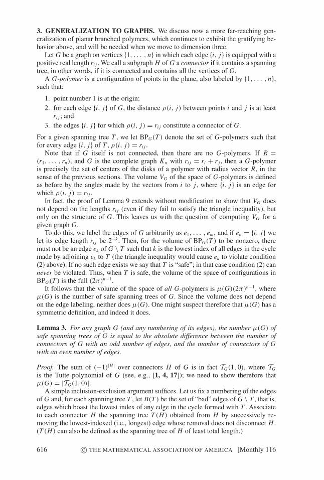
for short—is a connected set of n labeled unit spheres with nonoverlapping interiors.We will assume that the sphere labeled 1 is centered at the origin. See Figure 1 for anexample in the plane.

6

75

2

4

13

Figure 1. A branched polymer in the plane.

Intended as models in chemistry or biology, branched polymers are often modeled,in turn, by lattice animals (trees on a grid); see, e.g., [3, 5, 8, 10, 18, 19]. However,continuum polymers turn out to be in some respects more tractable than their gridcousins.

In order to study the behavior of branched polymers, and in particular to define andunderstand what random examples look like, we must define a parametrization andthen attempt to compute, using that parametrization, volumes of various configurationspaces. In principle, we could then compute (say) the probability that a branched poly-mer of a particular size in a given dimension takes the form of a specific tree, or hasdiameter exceeding some number; and we could perhaps generate uniformly randomexamples in an efficient manner.

Fortunately, the space of branched polymers of order n and dimension D possessesan obvious and natural parametrization. One of several equivalent ways to describe it isto specify the tree-type of the polymer, together with the n − 1 D-dimensional anglesat which each ball is attached to the next ball on the way to the root. This causes anambiguity if the polymer contains a cycle of touching balls (thus has multiple spanningtrees), but such polymers will have probability zero, so we don’t mind if they areparametrized in more than one way.

For example, in the plane, the set of polymers with two balls (disks) is parametrizedby a single angle at the origin (center of ball 1), measured counterclockwise from thex-axis to the center of ball 2. The volume of the configuration space is thus 2π .

612 c© THE MATHEMATICAL ASSOCIATION OF AMERICA [Monthly 116

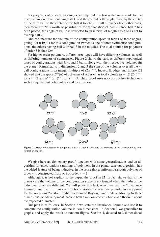
For polymers of order 3, two angles are required: the first is the angle made by thelowest-numbered ball touching ball 1, and the second is the angle made by the centerof the third ball to the center of the ball it touches. If ball 1 touches both other balls,then there are 2π’s worth of possibilities for the location of ball 2. Once ball 2 hasbeen placed, the angle of ball 3 is restricted to an interval of length 4π/3 so as not tooverlap ball 2.

One can measure the volume of the configuration space in terms of these angles,giving (2π)(4π/3) for this configuration (which is one of three symmetric configura-tions, the others having ball 2 or ball 3 in the middle). The total volume for polymersof order 3 is then 8π2.

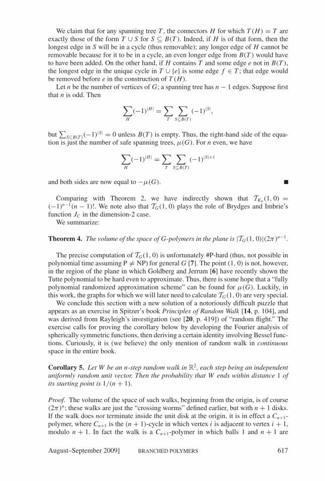
For higher-order polymers, different tree-types will have differing volumes, as wellas differing numbers of symmetries. Figure 2 shows the various different topologicaltypes of configurations with 3, 4, and 5 balls, along with their respective volumes (inthe plane). Remarkably, in dimensions 2 and 3 the sum of the volumes over all the n-ball configurations is an integer multiple of (2π)n−1. Indeed, Brydges and Imbrie [2]showed that the space B D(n) of polymers of order n has total volume (n − 1)! (2π)n−1

for D = 2 and nn−1(2π)n−1 for D = 3. Their proof uses nonconstructive techniquessuch as equivariant cohomology and localization.

Figure 2. Branched polymers in the plane with 3, 4, and 5 balls, and the volumes of the corresponding con-figuration spaces.

We give here an elementary proof, together with some generalizations and an al-gorithm for exact random sampling of polymers. In the planar case our algorithm hasthe added feature of being inductive, in the sense that a uniformly random polymer oforder n is constructed from one of order n − 1.

Although it is not explicit in the paper, the proof in [2] in fact shows that in theplanar case the volume of the configuration space is unchanged when the radii of theindividual disks are different. We will prove this fact, which we call the “InvarianceLemma,” and use it in our constructions. Along the way, we provide an easy prooffor the notorious “random flight” theorem of Rayleigh and Spitzer. Moving to threedimensions, our development leads to both a random construction and a theorem aboutthe expected diameter.

Our plan is as follows. In Section 2 we state the Invariance Lemma and use it tocompute the configuration volume in two dimensions. In Section 3 we generalize tographs, and apply the result to random flights. Section 4, devoted to 3-dimensional

August–September 2009] BRANCHED POLYMERS 613

polymers, uses the earlier results to compute volumes and diameter. Section 5 containsthe proof of the Invariance Lemma. Sections 6 and 7 show how to generate uniformlyrandom branched polymers in dimensions two and three. Finally, Section 8 gives someopen problems.

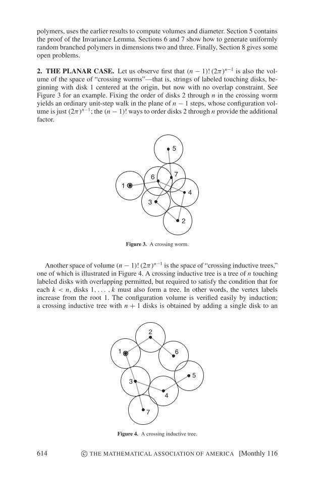
2. THE PLANAR CASE. Let us observe first that (n − 1)! (2π)n−1 is also the vol-ume of the space of “crossing worms”—that is, strings of labeled touching disks, be-ginning with disk 1 centered at the origin, but now with no overlap constraint. SeeFigure 3 for an example. Fixing the order of disks 2 through n in the crossing wormyields an ordinary unit-step walk in the plane of n − 1 steps, whose configuration vol-ume is just (2π)n−1; the (n − 1)! ways to order disks 2 through n provide the additionalfactor.

5

6 7

4

2

3

1

Figure 3. A crossing worm.

Another space of volume (n − 1)! (2π)n−1 is the space of “crossing inductive trees,”one of which is illustrated in Figure 4. A crossing inductive tree is a tree of n touchinglabeled disks with overlapping permitted, but required to satisfy the condition that foreach k < n, disks 1, . . . , k must also form a tree. In other words, the vertex labelsincrease from the root 1. The configuration volume is verified easily by induction;a crossing inductive tree with n + 1 disks is obtained by adding a single disk to an

1

7

4

5

6

3

2

Figure 4. A crossing inductive tree.


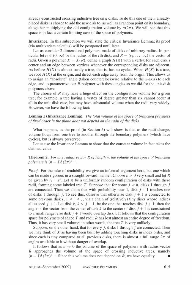
already-constructed crossing inductive tree on n disks. To do this one of the n already-placed disks is chosen to add the new disk to, as well as a random point on its boundary,altogether multiplying the old configuration volume by n(2π). We will see that thisspace is in fact a certain limiting case of the space of polymers.

Invariance. In this subsection we will state the critical Invariance Lemma; its proof(via multivariate calculus) will be postponed until later.

Let us consider 2-dimensional polymers made of disks of arbitrary radius. In par-ticular let ri ∈ (0, ∞) be the radius of the i th disk, and R = (r1, . . . , rn) the vector ofradii. Given a polymer X = X (R), define a graph H(X) with a vertex for each disk’scenter and an edge between vertices whenever the corresponding disks are adjacent.As before H(X) is almost surely a tree, that is, has no cycles. When H(X) is a tree,we root H(X) at the origin, and direct each edge away from the origin. This allows usto assign an “absolute” angle (taken counterclockwise relative to the x-axis) to eachedge, and to parametrize our R-polymer with these angles as we did for the unit-diskpolymers above.

The choice of R may have a huge effect on the configuration volume for a giventree; for example, a tree having a vertex of degree greater than six cannot occur atall in the unit-disk case, but may have substantial volume when the radii vary widely.However, we have the following fact:

Lemma 1 (Invariance Lemma). The total volume of the space of branched polymersof fixed order in the plane does not depend on the radii of the disks.

What happens, as the proof (in Section 5) will show, is that as the radii change,volume flows from one tree to another through the boundary polymers (which havecycles), but is always preserved.

Let us use the Invariance Lemma to show that the constant volume in fact takes theclaimed value.

Theorem 2. For any radius vector R of length n, the volume of the space of branchedpolymers is (n − 1)! (2π)n−1.

Proof. For the sake of readability we give an informal argument here, but one whichcan be made rigorous in a straightforward manner. Choose ε > 0 very small and let Rbe given by ri = εi . Let X be a uniformly random configuration of disks with theseradii, forming some labeled tree T . Suppose that for some j < n, disks 1 through jare connected. Then we claim that with probability near 1, disk j + 1 touches oneof disks 1 through j . To see this, observe that otherwise disk j + 1 is connected tosome previous disk i , 1 ≤ i ≤ j , via a chain of (relatively) tiny disks whose indicesall exceed j + 1. Let disk k, k > j + 1, be the one that touches disk j + 1; then theangle of the vector from the center of disk k to the center of disk j + 1 is constrainedto a small range, else disk j + 1 would overlap disk i . It follows that the configurationspace for polymers of shape T and radii R has lost almost an entire degree of freedom.Thus, it has very small volume; in other words, the tree T is very unlikely.

Suppose, on the other hand, that for every j , disks 1 through j are connected. Thenwe may think of X as having been built by adding touching disks in index order, andsince each is tiny compared to all previous disks, there is almost a full range 2π ofangles available to it without danger of overlap.

It follows that as ε → 0 the volume of the space of polymers with radius vectorR approaches the volume of the space of crossing inductive trees, namely(n − 1)! (2π)n−1. Since this volume does not depend on R, we have equality.


3. GENERALIZATION TO GRAPHS. We discuss now a more far-reaching gen-eralization of planar branched polymers, which continues to exhibit the gratifying be-havior above, and will be needed when we move to dimension three.

Let G be a graph on vertices {1, . . . , n} in which each edge {i, j} is equipped with apositive real length ri j . We call a subgraph H of G a connector if it contains a spanningtree, in other words, if it is connected and contains all the vertices of G.

A G-polymer is a configuration of points in the plane, also labeled by {1, . . . , n},such that:

1. point number 1 is at the origin;2. for each edge {i, j} of G, the distance ρ(i, j) between points i and j is at least

ri j ; and3. the edges {i, j} for which ρ(i, j) = ri j constitute a connector of G.

For a given spanning tree T , we let BPG(T ) denote the set of G-polymers such thatfor every edge {i, j} of T , ρ(i, j) = ri j .

Note that if G itself is not connected, then there are no G-polymers. If R =(r1, . . . , rn), and G is the complete graph Kn with ri j = ri + r j , then a G-polymeris precisely the set of centers of the disks of a polymer with radius vector R, in thesense of the previous sections. The volume VG of the space of G-polymers is definedas before by the angles made by the vectors from i to j , where {i, j} is an edge forwhich ρ(i, j) = ri j .

In fact, the proof of Lemma 9 extends without modification to show that VG doesnot depend on the lengths ri j (even if they fail to satisfy the triangle inequality), butonly on the structure of G. This leaves us with the question of computing VG for agiven graph G.

To do this, we label the edges of G arbitrarily as e1, . . . , em , and if ek = {i, j} welet its edge length ri j be 2−k . Then, for the volume of BPG(T ) to be nonzero, theremust not be an edge ek of G \ T such that k is the lowest index of all edges in the cyclemade by adjoining ek to T (the triangle inequality would cause ek to violate condition(2) above). If no such edge exists we say that T is “safe”; in that case condition (2) cannever be violated. Thus, when T is safe, the volume of the space of configurations inBPG(T ) is the full (2π)n−1.

It follows that the volume of the space of all G-polymers is μ(G)(2π)n−1, whereμ(G) is the number of safe spanning trees of G. Since the volume does not dependon the edge labeling, neither does μ(G). One might suspect therefore that μ(G) has asymmetric definition, and indeed it does.

Lemma 3. For any graph G (and any numbering of its edges), the number μ(G) ofsafe spanning trees of G is equal to the absolute difference between the number ofconnectors of G with an odd number of edges, and the number of connectors of Gwith an even number of edges.

Proof. The sum of (−1)|H | over connectors H of G is in fact TG(1, 0), where TG

is the Tutte polynomial of G (see, e.g., [1, 4, 17]); we need to show therefore thatμ(G) = |TG(1, 0)|.

A simple inclusion-exclusion argument suffices. Let us fix a numbering of the edgesof G and, for each spanning tree T , let B(T ) be the set of “bad” edges of G \ T , that is,edges which boast the lowest index of any edge in the cycle formed with T . Associateto each connector H the spanning tree T (H) obtained from H by successively re-moving the lowest-indexed (i.e., longest) edge whose removal does not disconnect H .(T (H) can also be defined as the spanning tree of H of least total length.)


We claim that for any spanning tree T , the connectors H for which T (H) = T areexactly those of the form T ∪ S for S ⊆ B(T ). Indeed, if H is of that form, then thelongest edge in S will be in a cycle (thus removable); any longer edge of H cannot beremovable because for it to be in a cycle, an even longer edge from B(T ) would haveto have been added. On the other hand, if H contains T and some edge e not in B(T ),the longest edge in the unique cycle in T ∪ {e} is some edge f ∈ T ; that edge wouldbe removed before e in the construction of T (H).

Let n be the number of vertices of G; a spanning tree has n − 1 edges. Suppose firstthat n is odd. Then ∑

H

(−1)|H | =∑

T

∑S⊆B(T )

(−1)|S|,

but∑

S⊆B(T )(−1)|S| = 0 unless B(T ) is empty. Thus, the right-hand side of the equa-tion is just the number of safe spanning trees, μ(G). For n even, we have∑

H

(−1)|H | =∑

T

∑S⊆B(T )

(−1)|S|+1

and both sides are now equal to −μ(G).

Comparing with Theorem 2, we have indirectly shown that TKn (1, 0) =(−1)n−1(n − 1)!. We note also that TG(1, 0) plays the role of Brydges and Imbrie’sfunction JC in the dimension-2 case.

We summarize:

Theorem 4. The volume of the space of G-polymers in the plane is |TG(1, 0)|(2π)n−1.

The precise computation of TG(1, 0) is unfortunately #P-hard (thus, not possible inpolynomial time assuming P = NP) for general G [7]. The point (1, 0) is not, however,in the region of the plane in which Goldberg and Jerrum [6] have recently shown theTutte polynomial to be hard even to approximate. Thus, there is some hope that a “fullypolynomial randomized approximation scheme” can be found for μ(G). Luckily, inthis work, the graphs for which we will later need to calculate TG(1, 0) are very special.

We conclude this section with a new solution of a notoriously difficult puzzle thatappears as an exercise in Spitzer’s book Principles of Random Walk [14, p. 104], andwas derived from Rayleigh’s investigation (see [20, p. 419]) of “random flight.” Theexercise calls for proving the corollary below by developing the Fourier analysis ofspherically symmetric functions, then deriving a certain identity involving Bessel func-tions. Curiously, it is (we believe) the only mention of random walk in continuousspace in the entire book.

Corollary 5. Let W be an n-step random walk in R2, each step being an independent

uniformly random unit vector. Then the probability that W ends within distance 1 ofits starting point is 1/(n + 1).

Proof. The volume of the space of such walks, beginning from the origin, is of course(2π)n; these walks are just the “crossing worms” defined earlier, but with n + 1 disks.If the walk does not terminate inside the unit disk at the origin, it is in effect a Cn+1-polymer, where Cn+1 is the (n + 1)-cycle in which vertex i is adjacent to vertex i + 1,modulo n + 1. In fact the walk is a Cn+1-polymer in which balls 1 and n + 1 are


not adjacent. Since μ(Cn+1) = |1 − (n + 1)| = n, the volume of the space of Cn+1-polymers is n(2π)n. Since the spanning tree with no edge between nodes 1 and n + 1is one of n + 1 symmetric choices, the volume of the Cn+1-polymers which correspondto non-returning random walks is n(2π)n/(n + 1), and the result follows.

4. THE 3-DIMENSIONAL CASE

Volume invariance. Branched polymers in 3-space share many of the features of pla-nar branched polymers. Brydges and Imbrie showed in [2] that the volume of theconfiguration space of polymers in 3-space is nn−1(2π)n−1. Here the volume is mea-sured in terms of the spherical angles, that is, the surface area measure on the spheres.Whereas the planar configuration space volume was independent of the radii of theballs, the same is not true in 3 dimensions.

One-dimensional projections. Let X be a branched polymer in R3 with ball centers

v1, . . . , vn . It will be convenient to assume that spheres of which our polymers arecomposed have diameter 1 instead of radius 1; thus the distance between any twosphere centers is at least 1, with equality in a spanning tree.

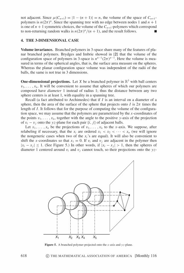
Recall (a fact attributed to Archimedes) that if I is an interval on a diameter of asphere, then the area of the surface of the sphere that projects onto I is 2π times thelength of I . It follows that for the purpose of computing the volume of the configura-tion space, we may assume that the polymers are parametrized by the x-coordinates ofthe points v1, . . . , vn, together with the angle to the positive y-axis of the projectionof vi − v j onto the yz-plane for each pair {i, j} of adjacent balls.

Let x1, . . . , xn be the projections of v1, . . . , vn to the x-axis. We suppose, afterrelabeling if necessary, that the xi are ordered x1 < x2 < · · · < xn (we will ignorethe nongeneric cases when two of the xi ’s are equal). It will also be convenient toshift the x-coordinates so that x1 = 0. If vi and v j are adjacent in the polymer then|xi − x j | ≤ 1. (See Figure 5.) In other words, if |xi − x j | > 1, then the spheres ofdiameter 1 centered around vi and v j cannot touch, so their projections onto the yz-

X1 X2 X3 X4 X5

Figure 5. A branched polymer projected onto the x-axis and yz-plane.


plane are unconstrained. If |xi − x j | ≤ 1 then the yz-projections of vi and v j cannotbe too close, else the corresponding spheres would overlap.

It follows that once x1 < x2 < · · · < xn are fixed, the allowable projections of thesphere centers on the yz-plane are exactly the G-polymers on that plane, for an ap-propriate choice of the graph G. Our plan for computing the total volume of the spaceof order-n polymers in R

3 is to use Theorem 4 to compute the (lower-dimensional)volume of the space of polymers with given x-axis projection, then integrate over allpossible x-axis projections. This seems more complicated than in the 2-dimensionalcase, but in fact gives us additional information.

Lemma 6. The (n − 1)-dimensional volume of the set of polymers whose centersproject to x1 < · · · < xn is an integer multiple of (2π)n−1 and depends only on theset of pairs i, j with |x j − xi | ≤ 1.

Proof. In any such polymer, the distance between the yz-plane projections of eachpair i, j of adjacent centers is determined by |xi − x j |; in fact the distance ri j satisfies(xi − x j )

2 + r 2i j = 1. For nonadjacent centers, this distance is at least ri j provided

|xi − x j | ≤ 1; otherwise it is unconstrained.It follows that if we let G be the graph on vertices {1, . . . , n} in which i is ad-

jacent to j if and only if |xi − x j | ≤ 1, then by Theorem 4 the desired volume isμ(G)(2π)n−1, where μ(G) = |TG(1, 0)|.Computing the volume. A unit interval graph (see, e.g., [12]) is defined by a setof unit-length intervals on the real line; it has one vertex for each interval and twointervals are adjacent in the graph just when they overlap. The graph G in the aboveproof is such a graph, with the intervals centered at the xi .

The value |TG(1, 0)| is easy to compute for unit interval graphs. Order the edges lex-icographically according to their (ordered) endpoints; that is, edge {i, j} (with i < j)precedes edge {i ′, j ′} (with i ′ < j ′) if i < i ′ or if i = i ′ and j < j ′. With this ordering,the safe spanning trees of G are those which are inductive in the sense of the intro-duction: all paths from the root 1 have increasing indices. It follows that each vertexj > 1 has as its parent some i < j for which x j − xi ≤ 1. Thus,

μ(G) =n∏

j=2

γ ( j) ,

where γ ( j) is the number of i < j for which x j − xi ≤ 1.It follows that the volume of the 3-dimensional polymer configuration space is

Vol(BPKn ) = (2π)n−1

∫D

n! μ(G) dx2 · · · dxn

= (2π)n−1

∫D

n!n∏

j=2

γ ( j) dx2 · · · dxn. (1)

Here the n! factor appears because of the relabelling of the balls, D is the domaindefined by {0 = x1 ≤ x2 ≤ · · · ≤ xn} and G is the interval graph defined from {0 =x1, x2, . . . , xn}.

Let Tn be a uniformly random tree on the labels {1, . . . , n}, with an independentuniformly random real length ui j in [0, 1] assigned to each edge {i, j}. Choose a rootfor Tn uniformly at random. For each j = 1, . . . , n let a j be the sum of the lengths of


the edges in the path from the root to j in T ; and let 0 = b1 ≤ b2 ≤ · · · ≤ bn be the ai

taken in order. Let B be the (random) vector (b1, . . . , bn).

Theorem 7. The total volume of the configuration space of 3-dimensional branchedpolymers of order n is nn−1(2π)n−1. Moreover, if X be a random branched polymer,and x1 ≤ x2 ≤ · · · ≤ xn the projections of its centers onto the x-axis, then, after trans-lating so that x1 = 0, the random vector (x1, x2, x3, . . . , xn) is distributed exactly as B.

Proof. Given the points 0 = x1 < · · · < xn , construct a labeled tree rooted at vertex 1by attaching each vertex j to some i < j satisfying |xi − x j | ≤ 1; there are

∏nj=2 γ ( j)

ways to do this. We can think of each such tree as having edge lengths given by the|xi − x j |.

If we then arbitrarily reassign labels {1, 2, . . . , n} to the vertices, we obtainn! ∏n

j=2 γ ( j) trees in all, each bearing the same relation to the x1, . . . , xn that thetrees Tn considered above have to b1, . . . , bn . We can evaluate the integral in (1) bycomputing the sum over these labeled trees of the integral over the set of x2, . . . , xn

which can give rise to that tree. However, the set of x2, . . . , xn which can give rise toa given labeled tree has volume exactly 1, since each edge of the tree can have anylength in [0, 1], independently of the others. Thus, each labeled tree contributes thesame amount, 1, to the integral.

By Cayley’s theorem (see, e.g., [9, Chapter 2]), the number of rooted labeled treeson n nodes is nn−1. Thus Vol(BPKn ) = (2π)n−1nn−1.

Since each tree contributes the same amount to the total volume, the second state-ment follows.

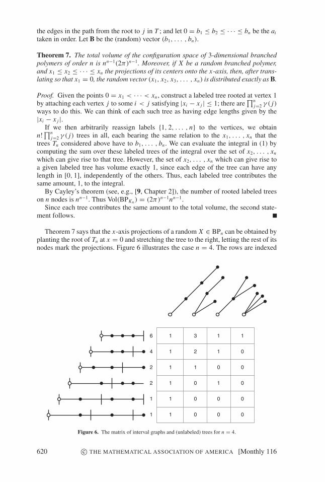
Theorem 7 says that the x-axis projections of a random X ∈ BPn can be obtained byplanting the root of Tn at x = 0 and stretching the tree to the right, letting the rest of itsnodes mark the projections. Figure 6 illustrates the case n = 4. The rows are indexed

6

4

2

2

1

1

1

1

1

1

1

1

3

2

1

0

0

0

1

1

0

1

0

0

1

0

0

0

0

0

Figure 6. The matrix of interval graphs and (unlabeled) trees for n = 4.


by interval graph types G, presented as sample projections, each accompanied by itsrelative volume μ(G). The columns are indexed by trees, each weighted by the numberof ways it can arise from an interval graph.

Note that the theorem does not say that the tree structure of a random 3-dimensionalpolymer is uniformly random; for example, no polymer can have a node of degreegreater than 12.

From Theorem 7 we can incidentally deduce the nonobvious fact that the “reverse”vector (0, bn − bn−1, bn − bn−2, . . . , bn) has the same distribution as B.

Theorem 8. The expected diameter (combinatorial or Euclidean) of a random 3-dimensional polymer grows as n1/2.

Proof. Szekeres’ Theorem (see [11, 16]) says that the expected length of the longestpath in a random tree on n labels is of order

√n. The expected length of the longest

path from the root in our edge-weighted tree Tn must therefore also be of order√

n, andthis is exactly the length of the projection of our random polymer on the x-axis. Sincethe space of polymers is independent of the choice of axes, the spatial diameter of arandom polymer must also be of order

√n. (If the diameter were significantly larger

than the diameter of its projection to the x-axis, then almost all random rotations ofthe polymer would result in a longer x-axis diameter.)

5. PROOF OF THE INVARIANCE LEMMA. We now return to the InvarianceLemma, which states that the volume of the space of planar polymers of order n doesnot depend on their radii. As noted above, the proof works for the more general G-polymer case as well.

Recall that given a polymer X = X (R), with radius vector R, the graph H(X)

has a vertex at the center of each disk and an edge between vertices whenever thecorresponding disks are adjacent. When (as almost surely) H(X) is a tree, we rootH(X) at the origin, and direct each edge away from the origin. Let e1, . . . , en−1 bethe edges of H(X) (chosen in some order) and θ1, . . . , θn−1 the corresponding “edgeangles.”

For a given combinatorial tree T (with labeled vertices), the set of polymers X =X (R, T ) with graph H(X) = T can thus be identified with a subset of [0, 2π)n−1. Callthis set BPR(T ) (this is shorthand notation for BPKn(R)). The boundary of BPR(T )

corresponds to polymers having at least one cycle; the corresponding plane graphsH(X) are obtained by adding one or more edges to T . Indeed, the boundary of BPR(T )

is piecewise smooth and the pieces of codimension k correspond to polymers with kelementary cycles (i.e., k edges must be removed from H to make a tree).

A polymer X with cycles lies in the boundary of each BPR(T ) for which T is a span-ning tree of the graph H(X). Each such BPR(T ) will contribute its own parametriza-tion to X . Note, however, that some trees may be unrealizable by unit disks (e.g., thestar inside a 6-wheel); for such trees T , BPR(T ) has zero volume.

We can construct a model for the parameter space of all polymers of size n and diskradii R by taking a copy of BPR(T ) for each possible combinatorial type of tree, andidentifying boundaries as above. Note that the identification maps are in general ana-lytic maps on the angles: in a polygon with k vertices whose edges have fixed lengthsr1, . . . , rk , any two consecutive angles are determined analytically by the remainingk − 2 angles. This space is, however, difficult to understand on its own. Are there othercoordinates in which it has a nice geometric structure?


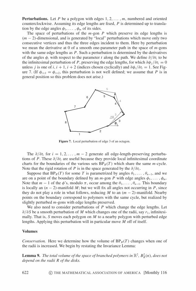
Perturbations. Let P be a polygon with edges 1, 2, . . . , m, numbered and orientedcounterclockwise. Assuming its edge lengths are fixed, P is determined up to transla-tion by the edge angles φ1, . . . , φm of its sides.

The space of perturbations of the m-gon P which preserve its edge lengths is(m − 2)-dimensional, and is generated by “local” perturbations which move only twoconsecutive vertices and thus the three edges incident to them. Here by perturbationwe mean the derivative at 0 of a smooth one-parameter path in the space of m-gonswith the same edge lengths as P . Such a perturbation is determined by the derivativesof the angles φi with respect to the parameter t along the path. We define ∂/∂ ti to bethe infinitesimal perturbation of P , preserving the edge lengths, for which ∂φ j/∂ ti = 0unless j is one of i, i + 1, i + 2 (indices chosen cyclically) and ∂φi/∂ ti = 1. See Fig-ure 7. (If φi+1 = φi+2, this perturbation is not well defined; we assume that P is ingeneral position so this problem does not arise.)

8

7

6 5

5

44

12

3

33

3

Figure 7. Local perturbation of edge 3 of an octagon.

The ∂/∂ ti for i = 1, 2, . . . , m − 2 generate all edge-length-preserving perturba-tions of P . These ∂/∂ ti are useful because they provide local infinitesimal coordinatecharts for the boundaries of the various sets BPR(T ) which share the same m-cycle.Note that the rigid rotation of P is in the space generated by the ∂/∂ ti .

Suppose that BPR(T ) for some T is parametrized by angles θ1, . . . , θn−1, and weare on a point of the boundary defined by an m-gon P with edge angles φ1, . . . , φm .Note that m − 1 of the φ’s, modulo π , occur among the θ1, . . . , θn−1. This boundaryis locally an (n − 2)-manifold M; but we will fix all angles not occurring in P , sincethey do not play a role in what follows, reducing M to an (m − 2)-manifold. Nearbypoints on the boundary correspond to polymers with the same cycle, but realized byslightly perturbed m-gons with edge lengths preserved.

We also need to consider perturbations of P which change the edge lengths. Let∂/∂S be a smooth perturbation of M which changes one of the radii, say r1, infinitesi-mally. That is, S moves each polygon on M to a nearby polygon with perturbed edgelengths. Applying this perturbation will in particular move M off of itself.

Volumes

Conservation. Here we determine how the volume of BPR(T ) changes when one ofthe radii is increased. We begin by restating the Invariance Lemma:

Lemma 9. The total volume of the space of branched polymers in R2, B2

R(n), does notdepend on the radii R of the disks.


Proof. We will prove the stronger fact that the local volume change under a smallchange in radii is zero. That is, near a polymer on the boundary of the configurationspace, the volumes of the parts of the configuration space lost or gained under a smallchange in radii sum to zero.

As above let P be an m-gon in a polymer in the boundary of BPR(T ). We canassume that P is the only cycle: otherwise we would be on a codimension-2 partof the boundary which will not contribute to the total volume change. Let M be the(m − 2)-manifold which is the part of the boundary of BPR(T ) near P when we havefixed the angles of all edges not in P . When we apply an infinitesimal perturbation tothe radii which increases r1, we can compute the change in the volume of BPR(T ) byintegrating, along the boundary, the infinitesimal change at each point on the boundary.We need, then, only compute the local volume element under the perturbation ∂

∂S . Wewill show that the sum of these local volume elements is zero.

Let A be an m × m square matrix whose first row is the all-ones vector, and forwhich det A = 0. Let B be the (m − 1) × m matrix obtained from A by removing thefirst row. Expanding 0 = det A along the first row, we deduce that the alternating sumof the (m − 1) × (m − 1) minors of B is zero: letting v j be the j th column vector ofB, we have

m∑j=1

(−1) jv1 ∧ · · · ∧ v j ∧ · · · ∧ vm = 0, (2)

where v j indicates that the entry v j is missing from the j th term, and v1 ∧ · · · ∧ v j ∧· · · ∧ vm denotes the determinant of the matrix whose columns are the v’s.

In the above let φ1, . . . , φm be the edge angles of the sides of P , and B the matrixwhose i j-entry is ∂φ j/∂ ti for i = 1, . . . , m − 2 and whose last row is ∂φ j/∂S forj = 1, . . . , m (see equation (3) below). Since the rigid rotation of P is in the spacegenerated by ∂φ j/∂ ti , the all-ones vector is a linear combination of the first m − 2rows of B. In particular the matrix A obtained from adding a row of 1’s to B hasdeterminant 0, and so we have (2).

We can, however, interpret the j th summand in (2), when integrated over M (andover the edges not included in P) as (up to sign, at least) the infinitesimal change involume of BPR(Tj ) under the perturbation S, where Tj runs over the trees obtainedby removing one edge of P . Once we have seen that the signs work out correctly,then, by (2), the net infinitesimal volume change of BPR(Tj ), when summed over j ,is zero.

Because of the factor (−1) j in (2), the signs work out correctly if and only if thevector ∂/∂ t1 ∧ · · · ∧ ∂/∂ tm−2 (by this we mean the cross product of these n − 2 vec-tors: the vector perpendicular to these and of length equal to their determinant on thesubspace they span) considered as a normal vector to the boundary of BPR(Tj ), rep-resents alternately the outward and inward normal to this boundary of BPR(Tj ) as jruns from 1 to m. In particular, we need to show that the orientation of this normalvector changes (from outward to inward or vice versa) when going from j to j + 1.To check this, take the vector ∂/∂Sj which increases (only) the radius r j of the ballbetween edges j and j + 1. This vector has positive component in the outward normaldirections for both BPR(Tj ) and BPR(Tj+1), since increasing the radius of the j th balldecreases the space available to Tj and Tj+1. However, ∂φi/∂Sj is zero unless i = jor j + 1 and the nonzero components ∂φ j/∂Sj and ∂φ j+1/∂Sj have opposite sign. Sothe two (m − 1) × (m − 1) minors of


⎛⎜⎜⎜⎜⎜⎜⎜⎜⎜⎜⎝

∂φ1

∂ t1. . .

∂φ j

∂ t1

∂φ j+1

∂ t1. . .

∂φm

∂ t1...

...

∂φ1

∂ tm−2. . .

∂φ j

∂ tm−2

∂φ j+1

∂ tm−2. . .

∂φm

∂ tm−2

0 . . .∂φ j

∂Sj

∂φ j+1

∂Sj0 . . . 0

⎞⎟⎟⎟⎟⎟⎟⎟⎟⎟⎟⎠

(3)

obtained by removing the j th or ( j + 1)st column have opposite sign. Therefore weneed to put in the sign change in (2) in order to make both represent the actual changesin the volumes of BPR(Tj) and BPR(Tj+1) under ∂/∂Sj (and therefore under any per-turbation of the radii).

Explicit formulae. The relative volume changes for the different BPR(Ti) as functionsof the shape of P have a surprisingly simple formula.

Proposition 10. Let P be an m-gon as above with edges e1, . . . , em in counterclock-wise order. The local volume change near P of BPR(Ti) due to an increase in radiusr1 (of the ball centered at the vertex between edges e1 and e2) is proportional to thedot product of ei and the vector w in direction 1

2 (φ1 + φ2), that is, perpendicular tothe angle bisector.

Note that since the vectors ei sum to zero, so do their dot products with w. Thisgives a restatement of the invariance principle.

Proof. Let Mi be the i th (m − 1) × (m − 1) minor of B, that is, Mi = v1 ∧ · · · ∧vi ∧ · · · ∧ vm . The vector V = (M1, −M2, M3, . . . , (−1)m+1 Mm) is in the kernel of B(since, upon adding a generic first row to B and inverting the resulting m × m matrix,the first column of the result is proportional to the above vector V ). Therefore V isperpendicular to the rows of B.

Write e j = a j eiφ j in polar coordinates. From∑

e j = 0 we get d(∑

e j

) =∑j a j ieiφ j dφ j = 0, or

∑j e j dφ j = 0 for any perturbation of the closed polygon

P fixing edge lengths. In particular the vector (e1, . . . , em) ∈ Cm is perpendicular

to the first m − 2 rows of B. Finally, let w be the vector ei(φ1+φ2)/2 and denote by〈e j , w〉 the component of e j in direction w. The vector (〈e1, w〉, 〈e2, w〉, . . . , 〈em, w〉)is perpendicular not just to the first m − 2 rows of B but also to the last row: thelast row is zero in all but the entries 1 and 2, and the values there are explicitly1

a1cot((φ1 − φ2)/2) and 1

a2cot((φ2 − φ1)/2) respectively.1

We therefore see that V is proportional to (〈e1, w〉, 〈e2, w〉, . . . , 〈em, w〉) asclaimed.

6. BUILDING RANDOM POLYMERS IN THE PLANE. We now show how toconstruct inductively a uniformly random branched polymer of order n in the plane.

We begin with a unit disk centered at the origin. Suppose we have constructed apolymer of size n − 1, n > 1. We choose a uniformly random disk from among then − 1 we have so far, then choose a uniformly random boundary point on that disk and

1This can be seen by taking ∂/∂S of the identity (a1 + S)eiφ1 + (a2 + S)eiφ2 = constant and solving for∂φ1/∂S, ∂φ2/∂S.


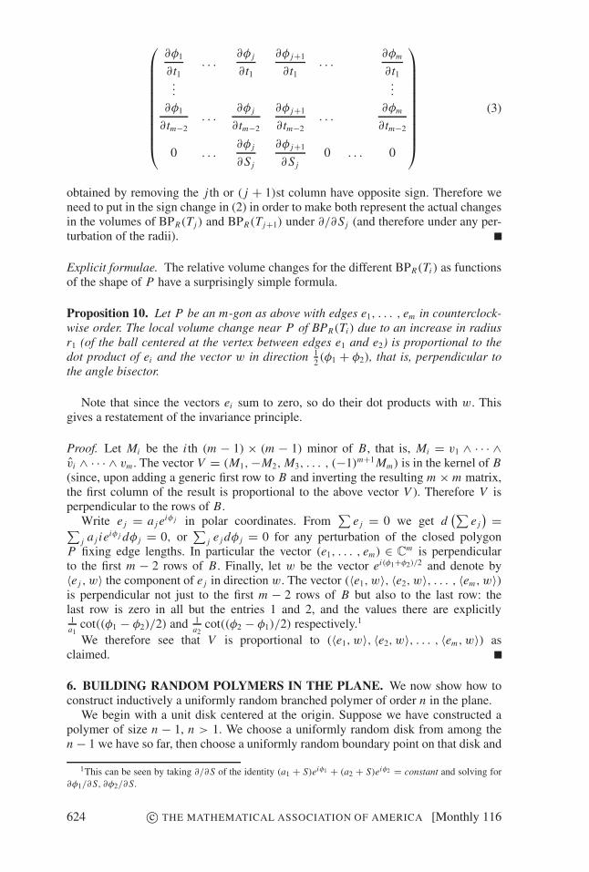
start growing a new disk tangent to that point. If a disk of radius 1 fits at that point,this will define a polymer of size n.

Otherwise there is a radius r with 0 < r < 1 at which a cycle P forms with the newdisk and some other disks present. At this point our polymer X is in the boundary of thespace BPR(T ), where R = {1, 1, . . . , 1, r}, and we need to choose some other tree T ′for which X is in the boundary of BPR(T ′), and which has the property that increasingr (and leaving the angles fixed) will not cause the disks to overlap. There will be atleast one possible such T ′ because the volume of BPR(T ) near X is decreasing as rincreases and so must be compensated by an increase in volume of some BPR(T ′).We choose randomly among the BPR(T ′) with increasing volume, with probabilityproportional to the infinitesimal change in the volumes of the BPR(T ′)’s as r increases.This ensures that the volume lost to BPR(T ) as r increases is distributed among theother BPR(T ′) so as to maintain the uniform measure.

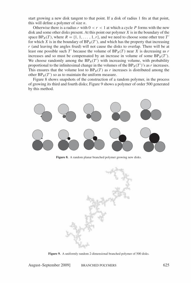
Figure 8 shows snapshots of the construction of a random polymer, in the processof growing its third and fourth disks; Figure 9 shows a polymer of order 500 generatedby this method.

Figure 8. A random planar branched polymer growing new disks.

Figure 9. A uniformly random 2-dimensional branched polymer of 500 disks.


All of the above is easily generalized to produce uniformly random G-polymersfor any connected graph G with specified edge lengths (and in fact we need this con-struction below, when generating 3-dimensional polymers). The vertices of G may betaken in any order v1, . . . , vn having the property that the subgraph Gk induced byv1, . . . , vk is connected for all k. When a uniformly random Gk−1-polymer has beenconstructed, a new point corresponding to vertex vk is added coincident to a pointuniformly chosen from its neighborhood—in other words, we start by assuming thatthe edges of Gk incident to vk are infinitesimal in length. These edges are then grownto their specified sizes, breaking cycles when they are formed in accordance with therules above.

7. CONSTRUCTING RANDOM POLYMERS IN 3-SPACE. To construct a uni-formly random 3-dimensional branched polymer of order n, we first select a uniformlyrandom labeled and rooted tree T from among the nn−1 possibilities. This can be doneby means of a Prufer code—see, e.g., [9]—which is itself just a sequence of n − 2numbers between 1 and n. The first entry of the code is the label of the vertex adjacentto the least-labeled leaf of T ; that leaf is then deleted and succeeding entries definedsimilarly. The reverse process is also unique and easy. After T is constructed, its rootk is chosen at random. In the constructed polymer, ball k will be the one whose centerhas least x-coordinate.

Edge-lengths are now chosen uniformly at random from [0, 1] for the edges of T ,and xi is set to be the length of the path from vertex i to the root k of T . The numbersx1, . . . , xn will be the projections onto the x-axis of the ball centers, shifted so that thecenter of ball k projects onto the origin.

The unit-interval graph H is defined as above on the tree vertices, namely byconnecting i to j if |x j − xi | ≤ 1. Edge lengths are assigned to H by (i, j) =√

1 − (x j − xi )2 so that the spheres of the polymer corresponding to tree vertices iand j are touching just when their centers lie at distance (i, j) when projected ontothe yz-plane, and in any case lie at least that far apart. From the argument in the proofof Theorem 7 we know that given x1, . . . , xn , the yz-plane projections are exactly auniformly random planar H -polymer, which is then constructed using the methods ofSection 6.

We now have the polymer’s yz-plane projection, as well as its (shifted) x-coordi-nates; it remains only to translate the polymer along the x-axis so that the center ofball 1 lies at the origin.

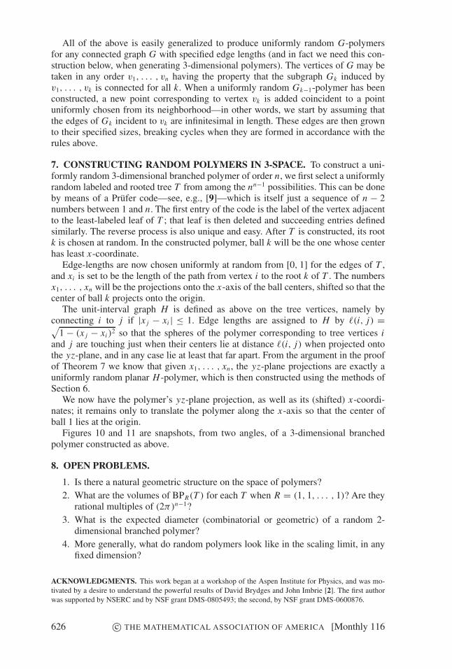
Figures 10 and 11 are snapshots, from two angles, of a 3-dimensional branchedpolymer constructed as above.

8. OPEN PROBLEMS.

1. Is there a natural geometric structure on the space of polymers?2. What are the volumes of BPR(T ) for each T when R = (1, 1, . . . , 1)? Are they

rational multiples of (2π)n−1?3. What is the expected diameter (combinatorial or geometric) of a random 2-

dimensional branched polymer?4. More generally, what do random polymers look like in the scaling limit, in any

fixed dimension?

ACKNOWLEDGMENTS. This work began at a workshop of the Aspen Institute for Physics, and was mo-tivated by a desire to understand the powerful results of David Brydges and John Imbrie [2]. The first authorwas supported by NSERC and by NSF grant DMS-0805493; the second, by NSF grant DMS-0600876.


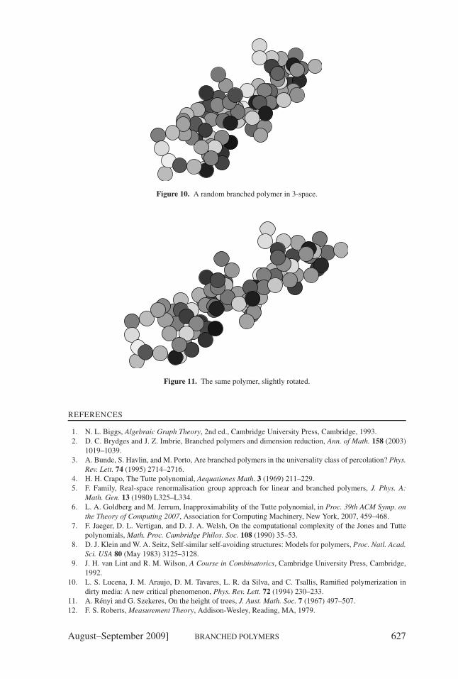
Figure 10. A random branched polymer in 3-space.

Figure 11. The same polymer, slightly rotated.

REFERENCES

1. N. L. Biggs, Algebraic Graph Theory, 2nd ed., Cambridge University Press, Cambridge, 1993.2. D. C. Brydges and J. Z. Imbrie, Branched polymers and dimension reduction, Ann. of Math. 158 (2003)

1019–1039.3. A. Bunde, S. Havlin, and M. Porto, Are branched polymers in the universality class of percolation? Phys.

Rev. Lett. 74 (1995) 2714–2716.4. H. H. Crapo, The Tutte polynomial, Aequationes Math. 3 (1969) 211–229.5. F. Family, Real-space renormalisation group approach for linear and branched polymers, J. Phys. A:

Math. Gen. 13 (1980) L325–L334.6. L. A. Goldberg and M. Jerrum, Inapproximability of the Tutte polynomial, in Proc. 39th ACM Symp. on

the Theory of Computing 2007, Association for Computing Machinery, New York, 2007, 459–468.7. F. Jaeger, D. L. Vertigan, and D. J. A. Welsh, On the computational complexity of the Jones and Tutte

polynomials, Math. Proc. Cambridge Philos. Soc. 108 (1990) 35–53.8. D. J. Klein and W. A. Seitz, Self-similar self-avoiding structures: Models for polymers, Proc. Natl. Acad.

Sci. USA 80 (May 1983) 3125–3128.9. J. H. van Lint and R. M. Wilson, A Course in Combinatorics, Cambridge University Press, Cambridge,

1992.10. L. S. Lucena, J. M. Araujo, D. M. Tavares, L. R. da Silva, and C. Tsallis, Ramified polymerization in

dirty media: A new critical phenomenon, Phys. Rev. Lett. 72 (1994) 230–233.11. A. Renyi and G. Szekeres, On the height of trees, J. Aust. Math. Soc. 7 (1967) 497–507.12. F. S. Roberts, Measurement Theory, Addison-Wesley, Reading, MA, 1979.


13. D. Ruelle, Existence of a phase transition in a continuous classical system, Phys. Rev. Lett. 27 (1971)1040–1041.

14. F. Spitzer, Principles of Random Walk, Van Nostrand, Princeton, NJ, 1964.15. R. Stanley, Enumerative Combinatorics, vol. I, Wadsworth & Brooks/Cole, Monterey, CA, 1986.16. G. Szekeres, Distribution of labeled trees by diameter, in Combinatorial Mathematics X, Lecture Notes

in Mathematics, vol. 1036, Springer-Verlag, New York, 1982.17. W. T. Tutte, Graph Theory, Addison-Wesley, Reading, MA, 1984.18. C. Vanderzande, Lattice Models of Polymers, Cambridge Lecture Notes in Physics, No. 11, Cambridge

University Press, Cambridge, 1998.19. D. Vujic, Branched polymers on the two-dimensional square lattice with attractive surfaces, J. Statist.

Phys. 95 (1999) 767–774.20. G. N. Watson, A Treatise on the Theory of Bessel Functions, 2nd ed., Cambridge University Press, Cam-

bridge, 1944.

RICHARD KENYON is Professor of Mathematics at Brown University. He held previous positions at theCNRS in Orsay, France and at the University of British Columbia. His interests include tilings, geometry,probability, and disc sports.Mathematics Department, Brown University, Providence RI 02912, [email protected]

PETER WINKLER is Professor of Mathematics and Computer Science, and Albert Bradley Third CenturyProfessor in the Sciences, at Dartmouth. His research is mostly in discrete mathematics and the theory ofcomputing; he has also written two books on mathematical puzzles, and in some circles is best known for hisinvention of cryptologic techniques for the game of bridge.Department of Mathematics, Dartmouth College, Hanover NH 03755-3551, [email protected]

Emily Dickinson and the Binomial Theorem

“I fancy you very often descending to the schoolroom with a plump BinomialTheorem struggling in your hand which you must dissect and exhibit to yourincomprehending ones.”

—Emily Dickinson, letter to her friend Susan Gilbert, Oct. 9, 1851.

At the time, Susan was teaching mathematics at Robert Archer’s school forgirls in Baltimore, MD. She married Emily’s brother Austin in 1856. Accordingto Susan’s obituary, “as a young woman [she] was so good in mathematics thatProf. Hadley of Yale (the father of President Hadley), who for a time gave herinstruction, told her that she ought to go to Yale college.”

The quotation from Emily’s letter can be found in T. H. Johnson, ed., The Let-ters of Emily Dickinson, Belknap Press, Cambridge, MA, 1958, p. 144. SusanGilbert Dickinson’s obituary is available at http://www.emilydickinson.org/

susan/obit.html.


Documents

Branched Polymers - Dartmouth Collegepw/papers/polymer.pdfBranched Polymers Richard Kenyon and Peter Winkler 1. INTRODUCTION. A branched polymer of order n in RD—or just “polymer”