Brazilian test: stress ﬁeld and tensile strength of ...simincoke.co/wp-content/uploads/2017/03/Brazilian test stress field...International Journal of Rock Mechanics & MiningSciences39

International Journal of Rock Mechanics & Mining Sciences 39 (2002) 991–1004

Brazilian test: stress field and tensile strength of anisotropic rocksusing an analytical solution

J. Claessona,*, B. Bohlolib

aDepartment of Building Physics, Chalmers University of Technology, Sven Hultinsg 8, Gothenburg 41296, SwedenbMinistry of Science Research and Technology, Dr. Beheshti Avenue, Tehran, Iran

Accepted 11 September 2002

Abstract

Tensile strength of rock is among the most important parameters influencing rock deformability, rock crushing and blasting

results. To calculate the tensile strength from the indirect tensile (Brazilian) test, one must know the principal tensile stress, in

particular at the rock disc center, where a crack initiates. This stress can be assessed by an analytical solution. A study of this

solution for anisotropic (transversely isotropic) rock is presented.

The solution is given explicitly. The key expansion coefficients are obtained from a complex-valued 2� 2 matrix equation. The

convergence of the solution is greatly improved by a new procedure. It is shown that the dimensionless stress field depends only on

two intrinsic parameters, E0=E and b: The stress at the center of the disc is given in charts as a function of these parameters (and the

angle yb between the direction of applied force and the plane of transverse isotropy). Furthermore, a new, reasonably accurate,

approximate formula for the principal tension at the disc center, (0,0), is derived from the analytical solution:

sptð0; 0ÞDP

pRLðffiffiffiffiffiffiffiffiffiffiffiE=E04

pÞcosð2ybÞ �

cosð4ybÞ4

ðb � 1Þ� �

;

where

b ¼

ffiffiffiffiffiffiffiffiEE0

p2

1

G0 �2n0

E0

� �:

The elastic parameters of rock in two perpendicular directions were measured in the laboratory. The result of the stress analysis was

applied in calculating the indirect tensile strength of gneiss, which has a well-defined foliation plane (transversely isotropic). When

the results were compared with the tensile strength of rock obtained by using a conventional formula that assumes isotropic

material, there was a significant difference. Moreover, good agreement was observed for the tensile strength calculated from the

stress charts and the proposed formula, when compared with other published stress charts.

r 2002 Elsevier Science Ltd. All rights reserved.

1. Introduction

Indirect tensile (Brazilian) testing of rock cores is aneasy and common method for determining the tensilestrength of rock. Tensile strength is calculated in thistest by using an equation, which assumes isotropicmaterial properties. Since many rock types (e.g.metamorphic and sedimentary) are anisotropic, and inparticular transversely isotropic, it is necessary to find a

method for determining the tensile strength of thesetypes of rocks from the Brazilian test. Many researchers[1–3] have studied the tensile strength of anisotropicrocks by using the Brazilian test with the equation forisotropic material.

A comprehensive analytical solution for an aniso-tropic disc subjected to the Brazilian test was presentedby Amadei et al. [4]. It is based on a solution methodgiven by Lekhnitskii [5]. The calculation of stress andtensile strength of the anisotropic rock sample requiresthat the principal elastic constants E; E 0; n; n0 and G0 bedetermined (n=E ¼ n0=E0). Chen [6] presents in diagrams

*Corresponding author. Tel.: +46-31-772-1996; fax: +46-31-772-

1993.

1365-1609/02/$ - see front matter r 2002 Elsevier Science Ltd. All rights reserved.

PII: S 1 3 6 5 - 1 6 0 9 ( 0 2 ) 0 0 0 9 9 - 0

the principal stress at the center of a rock disc as afunction of the three dimensionless parameters E=E0; n0

and E=G0:The original objectives of this work were to study the

analytical solution of Lekhnitskii, Amadei et al. andChen, and to apply the results of the stress analysis tocalculate the tensile strength of anisotropic rockmaterial from laboratory tests.

The study resulted in a few improvements of thesolution method. The convergence of the series solutionwas improved greatly by a new procedure. The stress,strain and displacement can be calculated, even at thedisc periphery, with a high degree of accuracy andwithout any problems of convergence. The key expan-sion coefficients involve the solution of 4� 4 matrixequations (Eq. (24)), involving the real and imaginaryparts of Am and Bm). This equation is reduced to asimpler complex-valued 2� 2 matrix (Eq. (25)). Theanalytical solution shows that the dimensionless stressfield depends on only two intrinsic parameters (and onthe angle yb between the direction of the applied forceand the direction normal to the plane of transverseisotropy). The stress at the center of the disc may begiven in the form of charts. Finally, it was found thatfrom the analytical solution, new, quite good approx-imate formulas could be derived for the principaltension and compression at the disc center (Eqs. (36)and (37)). The tensile stress spt (0,0) at the center of thedisc can be obtained from either the charts or theapproximate formula, Eq. (36).

2. The Brazilian test

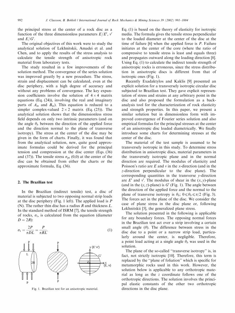
In the Brazilian (indirect tensile) test, a disc ofmaterial is subjected to two opposing normal strip loadsat the disc periphery (Fig. 1 left). The applied load is P

(N). The rather thin disc has a radius R and thickness L:In the standard method of ISRM [7], the tensile strengthof rocks, st; is calculated from the equation (diameterD ¼ 2R):

st ¼2P

pDL¼

P

pRL: ð1Þ

Eq. (1) is based on the theory of elasticity for isotropicmedia. The formula gives the tensile stress perpendicularto the loaded diameter at the center of the disc at thetime of failure [6] when the applied force is P: Failureinitiates at the center of the core (where the ratio ofcompressive to tensile stress is least and equals three)and propagates outward along the loading direction [8].Using Eq. (1) to calculate the indirect tensile strength ofanisotropic rocks is erroneous, since the stress distribu-tion in anisotropic discs is different from that ofisotropic ones (Fig. 1).

Recently Exadaktylos and Kaklis [9] presented anexplicit solution for a transversely isotropic circular discsubjected to Brazilian test. They gave explicit represen-tation of stress and strains at any arbitrary point in thedisc and also proposed the formulation as a back-analysis tool for the characterization of rock elasticityand strength properties. In this paper, we present asimilar solution but in dimensionless form with im-proved convergence of Fourier series solution and alsoempirical formulas for the principal stresses at the centerof an anisotropic disc loaded diametrically. We finallyintroduce some charts for determining stresses at thecenter of the disc.

The material of the test sample is assumed to betransversely isotropic in this study. To determine stressdistribution in anisotropic discs, material parameters inthe transversely isotropic plane and in the normaldirection are required. The modulus of elasticity andPoisson’s ratio are E and n in the x-direction (and in thez-direction perpendicular to the disc plane). Thecorresponding quantities in the transverse y-directionare E0 and n0: The modulus of shear in the (x; y)-plane(and in the (y; z)-plane) is G0 (Fig. 1). The angle betweenthe direction of the applied force and the normal to theplane of transverse isotropy is yb; 0pybpp/2 (Fig. 3).The forces act in the plane of the disc. We consider thecase of plane stress in the disc plane or, followingLekhnitskii [5], the generalized plane stress.

The solution presented in the following is applicablefor any boundary forces. The opposing normal forcesin the Brazilian test act over a strip involving a certainsmall angle (y). The difference between stress in thedisc due to a point or a narrow strip load, particu-larly around the center, is negligible. Therefore,a point load acting at a single angle yb was used in thesolution.

The plane of the so-called ‘‘transverse isotropy’’ is, infact, not strictly isotropic [10]. Therefore, this term isreplaced by the ‘‘plane of foliation’’ which is specific formetamorphic rocks used in this work. However, thesolution below is applicable to any orthotropic mate-rial as long as the z coordinate follows one of theorthotropic directions. The solution involves the princi-pal elastic constants of the other two orthotropicdirections in the disc plane.

P

L

P

2R

P

P

Z x(E, ν)

G'

y (E' ν')

Fig. 1. Brazilian test for an anisotropic material.

J. Claesson, B. Bohloli / International Journal of Rock Mechanics & Mining Sciences 39 (2002) 991–1004992

3. Problem to be solved

We consider plane stress in a transversely isotropicdisc. The basic equations to fulfill are force balance, therelation between strain and displacement, and Hooke’slaw:

qsx

qxþ

qtxy

qy¼ 0;

qtxy

qxþ

qsy

qy¼ 0; ð2Þ

ex ¼qu

qx; ey ¼

qv

qy; gxy ¼

qu

qyþ

qv

qx; ð3Þ

ex ¼sx

E�

n0sy

E0 ; ey ¼sy

E0 �n0sx

E0 ; gxy ¼txy

G0 : ð4Þ

It should be noted that n (¼ n0E=E0) does not appeardirectly in the above equations. The four elasticparameters that occur in the equations are E; E0; n0

and G0: The transversely isotropic disc has prescribedforces along its periphery. The boundary force FbðyÞ ¼ðXbðyÞ;YbðyÞÞ (N/m2) is a function of the angle y (Fig. 2).

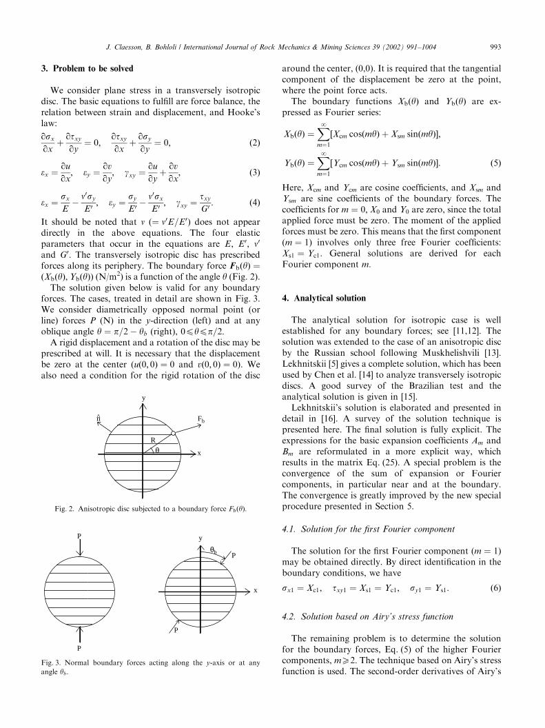
The solution given below is valid for any boundaryforces. The cases, treated in detail are shown in Fig. 3.We consider diametrically opposed normal point (orline) forces P (N) in the y-direction (left) and at anyoblique angle y ¼ p=2� yb (right), 0pypp=2:

A rigid displacement and a rotation of the disc may beprescribed at will. It is necessary that the displacementbe zero at the center (uð0; 0Þ ¼ 0 and vð0; 0Þ ¼ 0). Wealso need a condition for the rigid rotation of the disc

around the center, (0,0). It is required that the tangentialcomponent of the displacement be zero at the point,where the point force acts.

The boundary functions XbðyÞ and YbðyÞ are ex-pressed as Fourier series:

XbðyÞ ¼XNm¼1

½Xcm cosðmyÞ þ Xsm sinðmyÞ;

YbðyÞ ¼XNm¼1

½Ycm cosðmyÞ þ Ysm sinðmyÞ: ð5Þ

Here, Xcm and Ycm are cosine coefficients, and Xsm andYsm are sine coefficients of the boundary forces. Thecoefficients for m ¼ 0; X0 and Y0 are zero, since the totalapplied force must be zero. The moment of the appliedforces must be zero. This means that the first component(m ¼ 1) involves only three free Fourier coefficients:Xs1 ¼ Yc1: General solutions are derived for eachFourier component m:

4. Analytical solution

The analytical solution for isotropic case is wellestablished for any boundary forces; see [11,12]. Thesolution was extended to the case of an anisotropic discby the Russian school following Muskhelishvili [13].Lekhnitskii [5] gives a complete solution, which has beenused by Chen et al. [14] to analyze transversely isotropicdiscs. A good survey of the Brazilian test and theanalytical solution is given in [15].

Lekhnitskii’s solution is elaborated and presented indetail in [16]. A survey of the solution technique ispresented here. The final solution is fully explicit. Theexpressions for the basic expansion coefficients Am andBm are reformulated in a more explicit way, whichresults in the matrix Eq. (25). A special problem is theconvergence of the sum of expansion or Fouriercomponents, in particular near and at the boundary.The convergence is greatly improved by the new specialprocedure presented in Section 5.

4.1. Solution for the first Fourier component

The solution for the first Fourier component (m ¼ 1)may be obtained directly. By direct identification in theboundary conditions, we have

sx1 ¼ Xc1; txy1 ¼ Xs1 ¼ Yc1; sy1 ¼ Ys1: ð6Þ

4.2. Solution based on Airy’s stress function

The remaining problem is to determine the solutionfor the boundary forces, Eq. (5) of the higher Fouriercomponents, mX2: The technique based on Airy’s stressfunction is used. The second-order derivatives of Airy’s

θR

x

Fbn̂

y

Fig. 2. Anisotropic disc subjected to a boundary force FbðyÞ:

P

P

x

P

P

θb

y

Fig. 3. Normal boundary forces acting along the y-axis or at any

angle yb:

J. Claesson, B. Bohloli / International Journal of Rock Mechanics & Mining Sciences 39 (2002) 991–1004 993

function give the stress field

sx ¼ sx1 þq2F

qy2; sy ¼ sy1 þ

q2F

qx2; txy ¼ txy1 �

q2F

qxqy:

ð7Þ

These expressions fulfill the equations of force balance(2) for any sufficiently regular function F ðx; yÞ: Thecompatibility equation associated with Eqs. (2)–(4) givesthe following equation for F ðx; yÞ:

1

E0

q4F

qx4þ

1

G0 �2n0

E 0

� �q4F

qx2qy2þ

1

E

q4F

qy4¼ 0: ð8Þ

To obtain solutions to this equation, we use analyticalfunctions. Let f ðzÞ be an analytical function of thecomplex variable z ¼ x þ iy; and let m be a complex-valued constant. We choose the function

F ðx; yÞ ¼ f ðx þ myÞ: ð9Þ

Insertion of Eq. (9) in Eq. (8) gives the followingequation for F ðx; yÞ:

1

E0 � 1þ1

G0 �2n0

E0

� �m2 þ

1

Em4

� �d4f

dz4

��z¼xþmy

¼ 0:

The constant m is given by the roots of

m4 þ 2b

ffiffiffiffiffiE

E0

rm2 þ

E

E0 ¼ 0; b ¼


p2

1

G0 �2n0

E 0

� �: ð10Þ

Here, the critical new elastic constant b is introduced.Eq. (10) has (normally) four roots:m1; m2; m3 ¼ %m1; andm4 ¼ %m2: We have four solutions of the type f ðx þ mjyÞ;where fjðzÞ are free analytical functions. Actually twofree functions are needed to satisfy the two boundaryconditions. We choose

F ðx; yÞ ¼ 2 Re f1ðx þ m1yÞ þ f2ðx þ m2yÞ �

: ð11Þ

The above expression is a sufficiently general one tosolve our problem. Here, f1ðzÞ and f2ðzÞ are twoanalytical functions. The constants m1 and m2 (and theircomplex conjugates) are the roots of Eq. (10).

4.3. The roots m1 and m2

We need the roots of Eq. (10) which involve the twoparameters E0=E and b: The parameter b is defined inEq. (10). It is related to G0 and other elastic constants,and we may rewrite Eq. (10) in the following way:

G0 ¼E0

2ðbffiffiffiffiffiffiffiffiffiffiffiE=E0

pþ n0Þ

: ð12Þ

The roots of Eq. (10) are different for b > 1 and�1obo1: In an isotropic case, b ¼ 1 (E0=E ¼ 1 andG0 ¼ 0:5E=ð1þ n0Þ). The case bo� 1 is excluded, sincethe criterion of deformational stability is not fulfilled

[6,15,16,17]. For b > 1; we have

m1 ¼ iffiffiffiffiffiffiffiffiffiffiffiE=E04

p ffiffiffiffiffiffiffiffiffiffiffiffiffiffiffiffiffiffiffiffiffiffiffiffiffiffib þ

ffiffiffiffiffiffiffiffiffiffiffiffiffib2 � 1

pq;


p ffiffiffiffiffiffiffiffiffiffiffiffiffiffiffiffiffiffiffiffiffiffiffiffiffiffib �

ffiffiffiffiffiffiffiffiffiffiffiffiffib2 � 1

pq: ð13Þ

For 21obo1; we have


peijb=2; m2 ¼ i

ffiffiffiffiffiffiffiffiffiffiffiE=E 04

pe�ijb=2;

jb ¼ arccosðbÞ: ð14Þ

For b ¼ 1; the two roots m1 and m2 become equal. Thenthe solution below is not valid. This case ðb ¼ 1Þ is notdealt with here. Instead we may use the solution for b

close to 1 (for example b ¼ 1:001 or 0.999).

4.4. The stress field from Airy’s function

The stress and strain fields are obtained fromderivatives of F ðx; yÞ (Eq. (7)). Let F1ðzÞ and F2ðzÞdenote the complex-valued derivatives of f1ðzÞ and f2ðzÞ:

F1ðzÞ ¼df1

dz; F2ðzÞ ¼

df2

dzðz ¼ x þ iyÞ: ð15Þ

The stress components are obtained from Eqs. (6), (7)and (11):

sxðx; yÞ ¼ sx1 þ 2 Re m21F

01ðx þ m1yÞ þ m2

2F02ðx þ m2yÞ

�;

syðx; yÞ ¼ sy1 þ 2 Re F01ðx þ m1yÞ þ F0

2ðx þ m2yÞ �

;

txyðx; yÞ ¼ tyx1 � 2 Re m1F01ðx þ m1yÞ þ m2F

02ðx þ m2yÞ

�:

ð16Þ

Here, F0

1 and F0

2 denote the derivatives of the analyticalfunctions F1ðzÞ and F2ðzÞ taken at z ¼ x þ mjy; j ¼ 1; 2:

4.5. Boundary conditions

The stress field is expressed with two analyticalfunctions, F1 and F2; in the preceding two sections. Inthis section the boundary conditions for these twofunctions are formulated. We integrate these functionsin y: From this [6] we get, after an integration in y; thefollowing boundary conditions for the boundary func-tions, excluding the first component, m ¼ 1:Z y

0

Xbðy0Þ��mZ2

dy0 ¼2

RRe m1F1ðzb1Þ þ m2F2ðzb2Þ �

;

Z y

0

Ybðy0Þ��mZ2

dy0 ¼ �2

RRe F1ðzb1Þ þ F2ðzb2Þ½ : ð17Þ

Here, zb1ðyÞ and zb2ðyÞ are the arguments of F1 and F2

at the boundary of the disc:

zbjðyÞ ¼ R cosðyÞ þ mjR sinðyÞ; j ¼ 1; 2: ð18Þ

Let Xem and Yem be the complex-valued Fouriercoefficients for the integrals, Eq. (17), of the boundaryforces. They are related to the Fourier coefficients in


Eq. (5) in the following way:

Xem ¼Xcm � iXsm

2mi; Yem ¼

Ycm � iYsm

2mi: ð19Þ

From Eq. (17) it can be seen that our task is to find twoanalytical functions F1ðzÞ and F2ðzÞ so that

XNm¼2

Xem eimy þ %Xem e�imy �¼

2

RRe m1F1ðzb1Þ þ m2F2ðzb2Þ �

;

XNm¼2

Yem eimy þ %Yem e�imy �¼ �

2

RRe F1ðzb1Þ þ F2ðzb2Þ½ :

ð20Þ

4.6. Particular basic solutions

To fulfill Eq. (20), we need functions that vary asexpð7imyÞ at the periphery of the disc. The followingparticular set of basic functions will achieve this [5]:

Pj;mðzÞ ¼ ðWþj ðzÞÞm þ ðW�

j ðzÞÞm; m ¼ 1; 2; 3; y ;

Wþj ðzÞ ¼

z=R þ *RjðzÞ1� imj

; W�j ðzÞ ¼

z=R � *RjðzÞ1� imj

;

*RjðzÞ ¼ffiffiffiffiffiffiffiffiffiffiffiffiffiffiffiffiffiffiffiffiffiffiffiffiffiffiffiffiffiffiffiffiðz=RÞ2 � 1� m2

j

q; j ¼ 1; 2: ð21Þ

After some calculations, the values of Pj;m at theboundary of the disc become

Pj;mðzbjÞ ¼ eimy þ tmj e�imy; tj ¼

1þ imj

1� imj

; j ¼ 1; 2: ð22Þ

4.7. General series solution

A general solution for higher Fourier components(mX2) is now

F1ðzÞ ¼XNm¼2

AmP1;mðzÞ; F2ðzÞ ¼XNm¼2

BmP2;mðzÞ: ð23Þ

Here, Am and Bm (m ¼ 2; 3; y) are complex-valuedcoefficients to be determined by the boundary condi-tions. From Eqs. (21)–(23), the basic equations todetermine the expansion coefficients may be written inthe following way:

m1Am þ m2Bm þ m1tm1 Am þ m2tm

2 Bm ¼ RXem;

Am þ Bm þ tm1 Am þ tm

2 Bm ¼ �RYem: ð24Þ

These equations determine the expansion coefficients Am

and Bm from any given Xem and Yem: A crucial point isthat the ingenious choice of basic functions (21) resultsin decoupled equations. The solution for any m-level isindependent of the other levels.

4.8. The matrix equation for Am and Bm

The basic Eqs. (24) for the expansion coefficients mustbe fulfilled for both the real and imaginary parts. Theyinvolve four unknowns. The two equations may bewritten in matrix form, with Am and Bm; and theircomplex conjugates as unknowns. By considering thecomplex conjugate of the matrix equation, it is possibleto eliminate the complex conjugates of Am and Bm Fromthis we get the following matrix equation for thecoefficients Am and Bm [16]:

ðm1 � %m2Þð1� ðt1t1ÞmÞ ðm2 � %m2Þð1� ðt1 %t2Þ

mÞ

ð %m1 � m1Þð1� ðt1t1ÞmÞ ð %m1 � m2Þð1� ðt2 %t2Þ

mÞ

!Am

Bm

!

¼ RXem þ %m2Yem � %tm

1 ð %Xem þ %m2 %YemÞ

�Xem � %m1Yem � %tm2 ð %Xem þ %m1 %YemÞ

!

m ¼ 2; 3;y : ð25Þ

The determinant of the (2� 2)-matrix equation on theupper line is identically zero for m ¼ 1: This case is dealtwith separately in Section 4.1.

4.9. The stress field

The total stress field is given by Eq. (16). Here, F01 and

F02 denote the complex-valued derivatives of F1 and F2:

These functions are given by derivatives of the sums,Eq. (23):

F01ðzÞ ¼

XNm¼2

AmP01;mðzÞ; F0

2ðzÞ ¼XNm¼2

BmP02;mðzÞ: ð26Þ

The derivatives of Pj;mðzÞ become Eq. (21):

P0j;mðzÞ ¼

m

R

ðWþj ðzÞÞm � ðW�

j ðzÞÞm

*RjðzÞ; j ¼ 1; 2: ð27Þ

4.10. Fourier coefficients for normal point loads

The Fourier coefficients for opposing normal pointforces acting at the angles y ¼ p=2� yb and y ¼ �p=2�yb become Eqs. (5) and (19)

Xem ¼ pem sinðybÞeimyb ; Yem ¼ pem cosðybÞeimyb ;

pem ¼P

pRL

sinð0:5pmÞm

ðm ¼ 1; 2;yÞ: ð28Þ

The even coefficients are zero.

5. Improved convergence

It is a well-known experience that the convergence ofFourier series may be slow. The convergence of series(23) for the F-functions and their derivatives may alsobe quite slow, in particular at and near the boundary ofthe disc. Lekhnitskii [5] stresses the importance of this


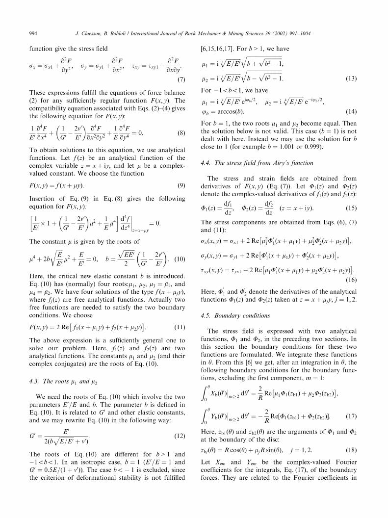
problem. The normal stress component at the peripheryof the disc, shown in Fig. 4, was calculated with termsup to m ¼ 9 and 15 (the even terms are zero). The loadat y ¼ p=2 becomes sharper as the number of termsincreases. We see that many terms are needed torepresent the boundary force. The number of oscilla-tions increases linearly with the number of terms. Butthe boundary value will always oscillate between 1 and�1 (for P ¼ pRL). The error at the center will decrease;however rather many terms are needed to get highaccuracy, in particular near the boundary.

The new procedure to obtain much better conver-gence is described in detail in [16]. Only the main ideasare indicated here. The absolute values of the constantst1 and t2; Eq. (22), are smaller than 1. They occur aspowers of m in Eq. (25), and they tend towards zero withincreasing m: We can get a simpler matrix equation bysetting these powers to zero in Eq. (25). The solutionEq. (26) to the difference between the true coefficientsfrom Eq. (25) and the simplified coefficients, when thepowers of t1 and t2 are set to zero, will then convergemuch better. To this solution we must add another onewith the simplified coefficients. It is shown in [15] thatthe latter solution may be expressed analytically as twointegrals involving the boundary forces Xb ðyÞ andYbðyÞ. These integrals are evaluated analytically. We getclosed-form analytical expressions for the solution withthe simplified coefficients.

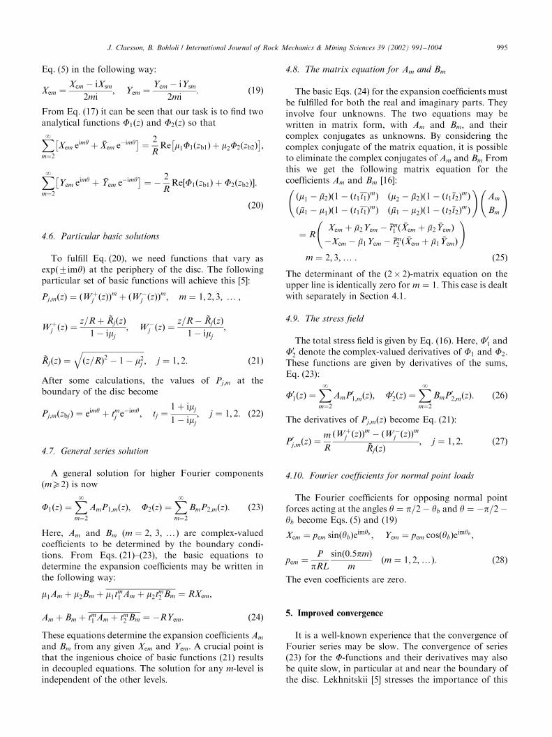
Fig. 5 shows the two components of the normal stressat the periphery of the disc using the terms up to m ¼ 7;

when the procedure for improved convergence is used.We see that the amplitude of the boundary oscillations isaround 2� 10�7; and that the point force is extremelysharp. It turns out to be quite sufficient to use the termsup to m ¼ 7 even directly at the boundary, and certainlyat the center, in the calculations of the stress field.

6. Summary of the general solution behavior

The solution for any boundary force is obtained fromthe formulas above in the following way. The Fouriercoefficients of the boundary forces are first calculated(Eq. (5)). The Fourier coefficients of the integrals of theboundary forces are given by Eq. (19). The constants inEq. (25) are obtained from Eqs. (10), (13), (14) and (22),and the expansion coefficients Am and Bm are deter-mined from Eq. (25). The stress field is given by Eqs. (6)and (16). The functions F1ðzÞ and F2ðzÞ are defined byEqs. (21) and (23), and their derivatives by Eqs. (26) and(27). The strain field is obtained from Hook’s relations,Eq. (4), and the displacement field from a straightfor-ward integration of Eq. (3) [16]. The solution is fullyexplicit for any boundary functions.

The solution for opposing normal point forces isobtained with the Fourier coefficients (Eq. (28)). Thissolution was implemented in the mathematical compu-ter program Mathcad. The procedure for improvedconvergence is included. In this type of program, it issimple to test directly whether the solution fulfills allconditions given by Eqs. (3)–(5) at any point. A goodtest is the independent direct calculation of theboundary force as shown in Figs. 4 and 5. An accuracyof, say 5 decimals, is obtained without difficulty. Thecalculation of the stress field with 10 000 points (Fig. 7)requires less than a minute or two of computer time on agood standard PC.

The following reference case will be used for thegraphical presentations of stress and displacement fields:

E ¼ 50:7; E0 ¼ 40; G0 ¼ 15:6 ðGPaÞ;

n0 ¼ 0:28; P ¼ pRL

) E0=E ¼ 0:789; b ¼ 1:126: ð29Þ

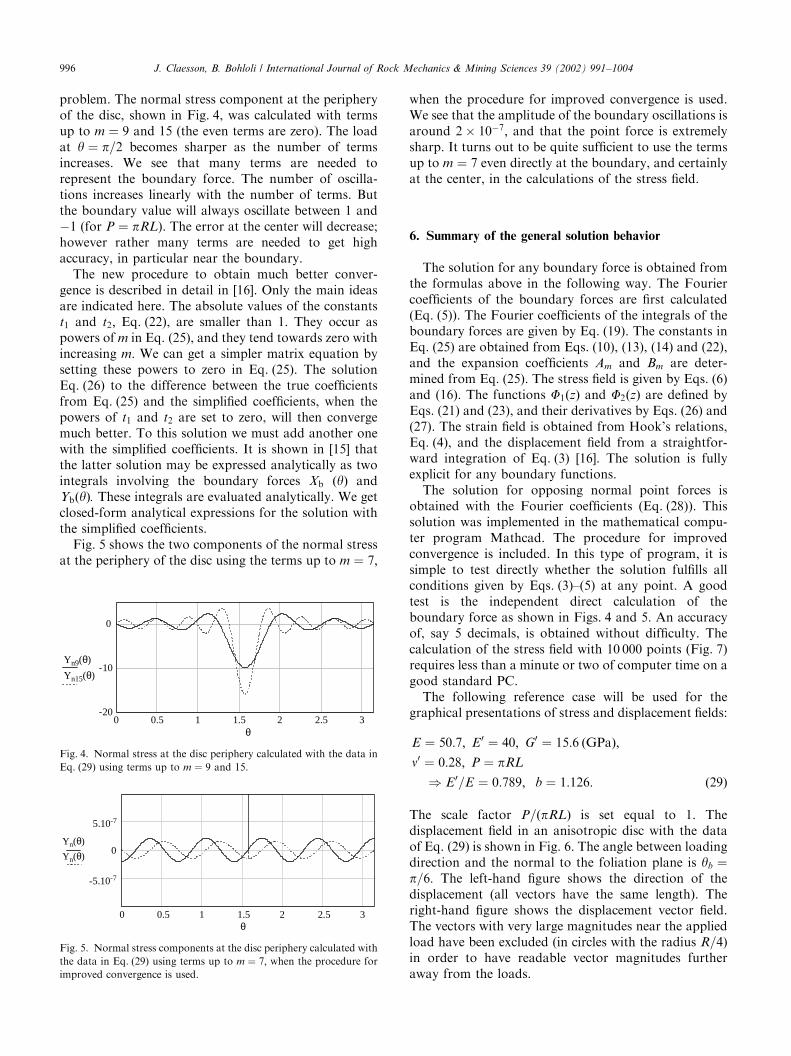
The scale factor P=ðpRLÞ is set equal to 1. Thedisplacement field in an anisotropic disc with the dataof Eq. (29) is shown in Fig. 6. The angle between loadingdirection and the normal to the foliation plane is yb ¼p=6: The left-hand figure shows the direction of thedisplacement (all vectors have the same length). Theright-hand figure shows the displacement vector field.The vectors with very large magnitudes near the appliedload have been excluded (in circles with the radius R=4)in order to have readable vector magnitudes furtheraway from the loads.

0 0.5 1 1.5 2 2.5 320

10

0

Yn9(θ)

Yn15(θ)

θ

Fig. 4. Normal stress at the disc periphery calculated with the data in

Eq. (29) using terms up to m ¼ 9 and 15.

0 0.5 1 1.5 2 2.5 3

0

5.10-7

-5.10-7

θ

Yn(θ)

Yn(θ)

Fig. 5. Normal stress components at the disc periphery calculated with

the data in Eq. (29) using terms up to m ¼ 7; when the procedure for

improved convergence is used.


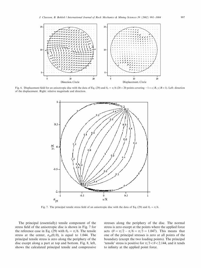
The principal (essentially) tensile component of thestress field of the anisotropic disc is shown in Fig. 7 forthe reference case in Eq. (29) with yb ¼ p=6: The tensilestress at the center, sptð0; 0Þ; is equal to 1.044. Theprincipal tensile stress is zero along the periphery of thedisc except along a part at top and bottom. Fig. 8, left,shows the calculated principal tensile and compressive

stresses along the periphery of the disc. The normalstress is zero except at the points where the applied forceacts (y ¼ p=2� p=6 ¼ p=3 ¼ 1:047). This means thatone of the principal stresses is zero at all points of theboundary (except the two loading points). The principal‘tensile’ stress is positive for p=3oyo2:144; and it tendsto infinity at the applied point force.

Fig. 6. Displacement field for an anisotropic disc with the data of Eq. (29) and yb ¼ p=6 (20� 20 points covering 21ox=R; y=Ro1). Left: direction

of the displacement. Right: relative magnitude and direction.

Fig. 7. The principal tensile stress field of an anisotropic disc with the data of Eq. (29) and yb ¼ p=6:


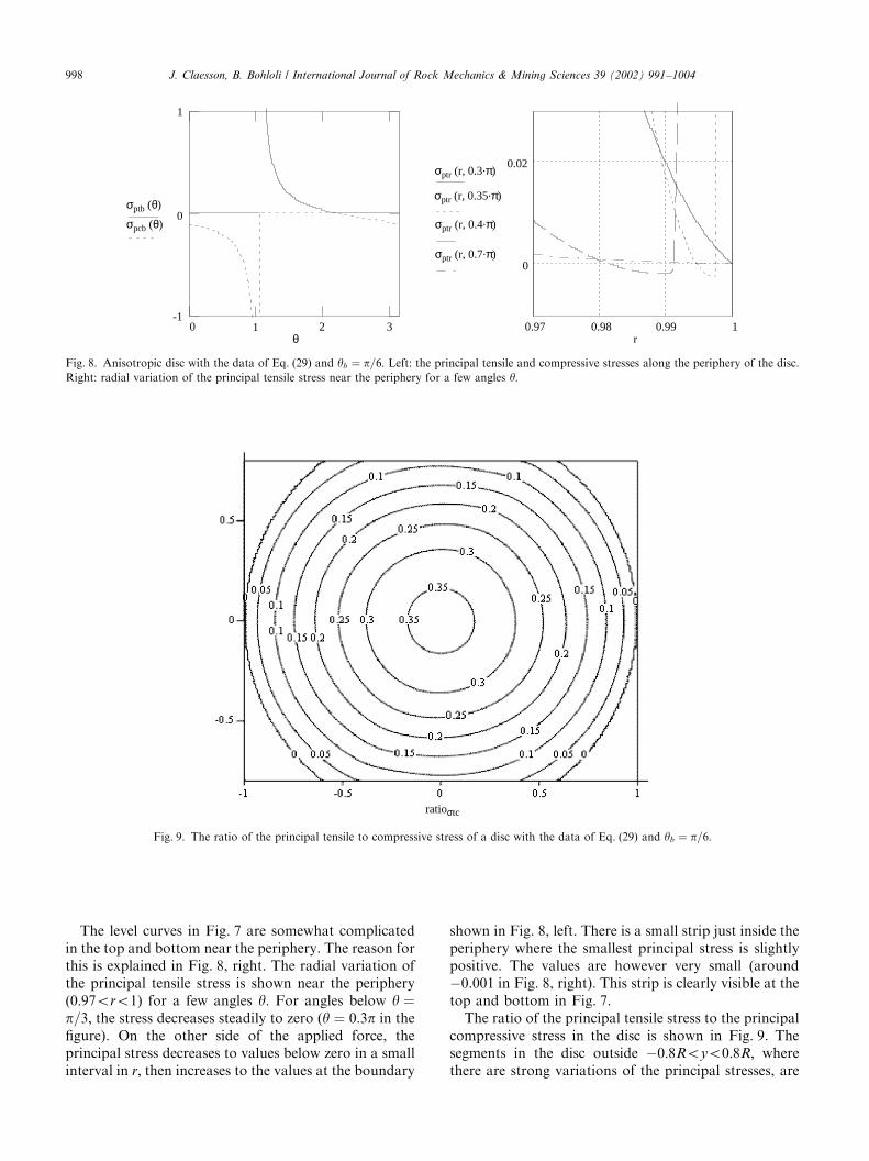
The level curves in Fig. 7 are somewhat complicatedin the top and bottom near the periphery. The reason forthis is explained in Fig. 8, right. The radial variation ofthe principal tensile stress is shown near the periphery(0:97oro1) for a few angles y: For angles below y ¼p=3; the stress decreases steadily to zero (y ¼ 0:3p in thefigure). On the other side of the applied force, theprincipal stress decreases to values below zero in a smallinterval in r; then increases to the values at the boundary

shown in Fig. 8, left. There is a small strip just inside theperiphery where the smallest principal stress is slightlypositive. The values are however very small (around�0.001 in Fig. 8, right). This strip is clearly visible at thetop and bottom in Fig. 7.

The ratio of the principal tensile stress to the principalcompressive stress in the disc is shown in Fig. 9. Thesegments in the disc outside �0:8Royo0:8R; wherethere are strong variations of the principal stresses, are

0 2 3-1

0

1

σptb (θ)

σpcb (θ)

θ0.97 0.98 0.99 1

0

0.02σptr (r, 0.3.π)

σptr (r, 0.35.π)

σptr (r, 0.4.π)

σptr (r, 0.7.π)

r1

Fig. 8. Anisotropic disc with the data of Eq. (29) and yb ¼ p=6: Left: the principal tensile and compressive stresses along the periphery of the disc.

Right: radial variation of the principal tensile stress near the periphery for a few angles y:

ratioσtc

Fig. 9. The ratio of the principal tensile to compressive stress of a disc with the data of Eq. (29) and yb ¼ p=6:


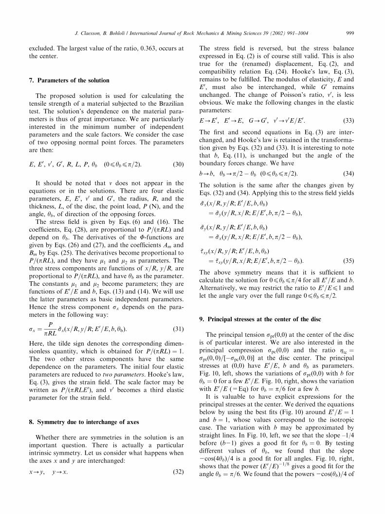
excluded. The largest value of the ratio, 0.363, occurs atthe center.

7. Parameters of the solution

The proposed solution is used for calculating thetensile strength of a material subjected to the Braziliantest. The solution’s dependence on the material para-meters is thus of great importance. We are particularlyinterested in the minimum number of independentparameters and the scale factors. We consider the caseof two opposing normal point forces. The parametersare then:

E; E0; n0; G0; R; L; P; yb ð0pybpp=2Þ: ð30Þ

It should be noted that n does not appear in theequations or in the solutions. There are four elasticparameters, E; E 0; n0 and G0; the radius, R; and thethickness, L; of the disc, the point load, P (N), and theangle, yb; of direction of the opposing forces.

The stress field is given by Eqs. (6) and (16). Thecoefficients, Eq. (28), are proportional to P=ðpRLÞ anddepend on yb: The derivatives of the F-functions aregiven by Eqs. (26) and (27), and the coefficients Am andBm by Eqs. (25). The derivatives become proportional toP=ðpRLÞ; and they have m1 and m2 as parameters. Thethree stress components are functions of x=R; y=R, areproportional to P=ðpRLÞ; and have yb as the parameter.The constants m1 and m2 become parameters; they arefunctions of E0=E and b; Eqs. (13) and (14). We will usethe latter parameters as basic independent parameters.Hence the stress component sx depends on the para-meters in the following way:

sx ¼P

pRL*sxðx=R; y=R;E0=E; b; ybÞ: ð31Þ

Here, the tilde sign denotes the corresponding dimen-sionless quantity, which is obtained for P=ðpRLÞ ¼ 1:The two other stress components have the samedependence on the parameters. The initial four elasticparameters are reduced to two parameters. Hooke’s law,Eq. (3), gives the strain field. The scale factor may bewritten as P=ðpRLE 0Þ; and n0 becomes a third elasticparameter for the strain field.

8. Symmetry due to interchange of axes

Whether there are symmetries in the solution is animportant question. There is actually a particularintrinsic symmetry. Let us consider what happens whenthe axes x and y are interchanged:

x-y; y-x: ð32Þ

The stress field is reversed, but the stress balanceexpressed in Eq. (2) is of course still valid. This is alsotrue for the (renamed) displacement, Eq. (2), andcompatibility relation Eq. (24). Hooke’s law, Eq. (3),remains to be fulfilled. The modulus of elasticity, E andE0; must also be interchanged, while G0 remainsunchanged. The change of Poisson’s ratio, n0, is lessobvious. We make the following changes in the elasticparameters:

E-E0; E0-E; G-G0; n0-n0E=E0: ð33Þ

The first and second equations in Eq. (3) are inter-changed, and Hooke’s law is retained in the transforma-tion given by Eqs. (32) and (33). It is interesting to notethat b; Eq. (11), is unchanged but the angle of theboundary forces change. We have

b-b; yb-p=2� yb ð0pybpp=2Þ: ð34Þ

The solution is the same after the changes given byEqs. (32) and (34). Applying this to the stress field yields

*sxðx=R; y=R;E0=E; b; ybÞ

¼ *syðy=R;x=R;E=E0; b; p=2� ybÞ;

*syðx=R; y=R;E0=E; b; ybÞ

¼ *sxðy=R;x=R;E=E0; b;p=2� ybÞ;

*txyðx=R; y=R;E0=E; b; ybÞ

¼ *txyðy=R;x=R;E=E0; b;p=2� ybÞ: ð35Þ

The above symmetry means that it is sufficient tocalculate the solution for 0pybpp=4 for all E0=E and b:Alternatively, we may restrict the ratio to E0=Ep1 andlet the angle vary over the full range 0pybpp=2.

9. Principal stresses at the center of the disc

The principal tension spt(0,0) at the center of the discis of particular interest. We are also interested in theprincipal compression spc(0,0) and the ratio Ztc ¼sptð0; 0Þ=½�spcð0; 0Þ at the disc center. The principalstresses at (0,0) have E0=E; b and yb as parameters.Fig. 10, left, shows the variations of spt(0,0) with b foryb ¼ 0 for a few E0=E. Fig. 10, right, shows the variationwith E0=E (=Eq) for yb ¼ p=6 for a few b.

It is valuable to have explicit expressions for theprincipal stresses at the center. We derived the equationsbelow by using the best fits (Fig. 10) around E0=E ¼ 1and b ¼ 1; whose values correspond to the isotropiccase. The variation with b may be approximated bystraight lines. In Fig. 10, left, we see that the slope –1/4before (b21) gives a good fit for yb ¼ 0. By testingdifferent values of yb; we found that the slope2cosð4ybÞ=4 is a good fit for all angles. Fig. 10, right,shows that the power ðE 0=EÞ21=8 gives a good fit for theangle yb ¼ p=6. We found that the powers 2cosðybÞ=4 of


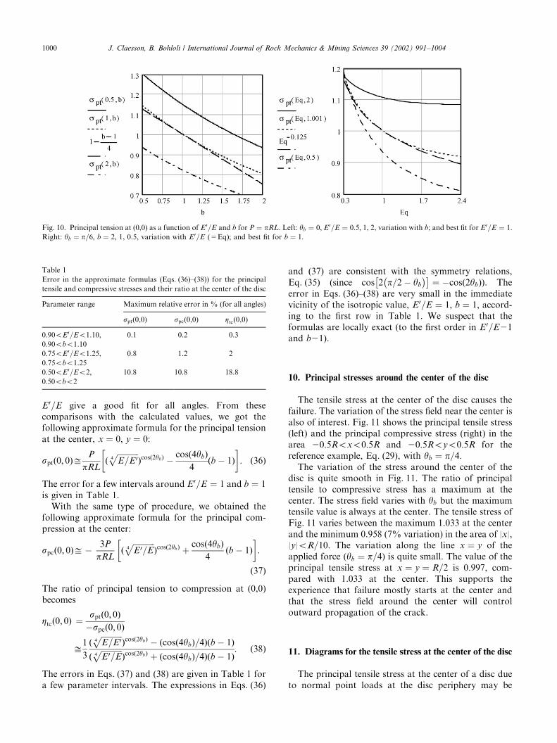
E0=E give a good fit for all angles. From thesecomparisons with the calculated values, we got thefollowing approximate formula for the principal tensionat the center, x ¼ 0; y ¼ 0:

sptð0; 0ÞDP


pÞcosð2ybÞ �

cosð4ybÞ4

ðb � 1Þ� �

: ð36Þ

The error for a few intervals around E0=E ¼ 1 and b ¼ 1is given in Table 1.

With the same type of procedure, we obtained thefollowing approximate formula for the principal com-pression at the center:

spcð0; 0ÞD�3P

pRLðffiffiffiffiffiffiffiffiffiffiffiE0=E4

pÞcosð2ybÞ þ

cosð4ybÞ4

ðb � 1Þ� �

:

ð37Þ

The ratio of principal tension to compression at (0,0)becomes

Ztcð0; 0Þ ¼sptð0; 0Þ�spcð0; 0Þ

D1

3

ðffiffiffiffiffiffiffiffiffiffiffiE=E04

pÞcosð2ybÞ � ðcosð4ybÞ=4Þðb � 1Þ

ðffiffiffiffiffiffiffiffiffiffiffiE0=E4

pÞcosð2ybÞ þ ðcosð4ybÞ=4Þðb � 1Þ

: ð38Þ

The errors in Eqs. (37) and (38) are given in Table 1 fora few parameter intervals. The expressions in Eqs. (36)

and (37) are consistent with the symmetry relations,Eq. (35) (since cos 2 p=2� yb

� � �¼ �cosð2ybÞ). The

error in Eqs. (36)–(38) are very small in the immediatevicinity of the isotropic value, E0=E ¼ 1; b ¼ 1; accord-ing to the first row in Table 1. We suspect that theformulas are locally exact (to the first order in E0=E21and b21).

10. Principal stresses around the center of the disc

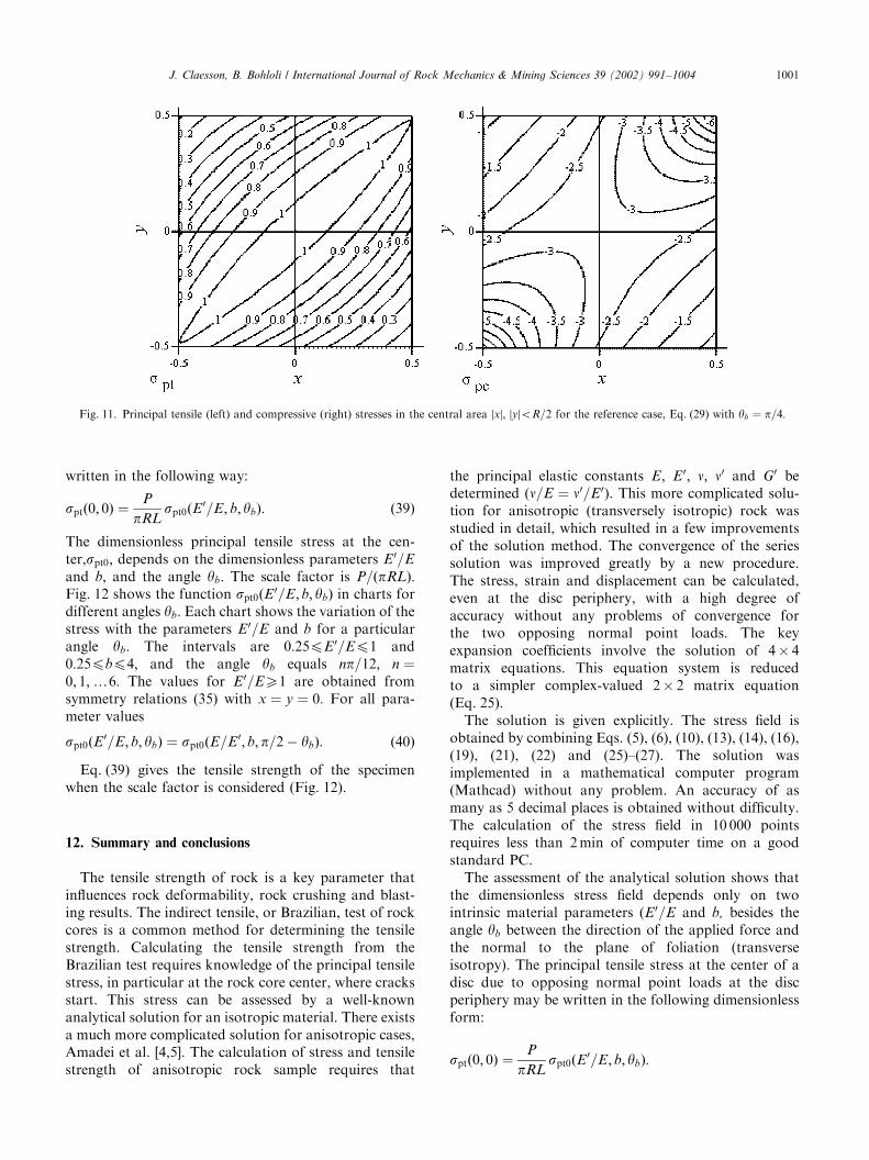
The tensile stress at the center of the disc causes thefailure. The variation of the stress field near the center isalso of interest. Fig. 11 shows the principal tensile stress(left) and the principal compressive stress (right) in thearea 20:5Roxo0:5R and 20:5Royo0:5R for thereference example, Eq. (29), with yb ¼ p=4:

The variation of the stress around the center of thedisc is quite smooth in Fig. 11. The ratio of principaltensile to compressive stress has a maximum at thecenter. The stress field varies with yb but the maximumtensile value is always at the center. The tensile stress ofFig. 11 varies between the maximum 1.033 at the centerand the minimum 0.958 (7% variation) in the area of |x|,|y|oR=10: The variation along the line x ¼ y of theapplied force (yb ¼ p=4) is quite small. The value of theprincipal tensile stress at x ¼ y ¼ R=2 is 0.997, com-pared with 1.033 at the center. This supports theexperience that failure mostly starts at the center andthat the stress field around the center will controloutward propagation of the crack.

11. Diagrams for the tensile stress at the center of the disc

The principal tensile stress at the center of a disc dueto normal point loads at the disc periphery may be

Table 1

Error in the approximate formulas (Eqs. (36)–(38)) for the principal

tensile and compressive stresses and their ratio at the center of the disc

Parameter range Maximum relative error in % (for all angles)

spt(0,0) spc(0,0) Ztc(0,0)

0.90oE0=Eo1.10,

0.90obo1.10

0.1 0.2 0.3

0.75oE0=Eo1.25,

0.75obo1.25

0.8 1.2 2

0.50oE0=Eo2;0:50obo2

10.8 10.8 18.8

Fig. 10. Principal tension at (0,0) as a function of E0=E and b for P ¼ pRL: Left: yb ¼ 0; E0=E ¼ 0:5; 1, 2, variation with b; and best fit for E0=E ¼ 1:Right: yb ¼ p=6; b ¼ 2; 1, 0.5, variation with E0=E (=Eq); and best fit for b ¼ 1:


written in the following way:

sptð0; 0Þ ¼P

pRLspt0ðE0=E; b; ybÞ: ð39Þ

The dimensionless principal tensile stress at the cen-ter,spt0; depends on the dimensionless parameters E0=E

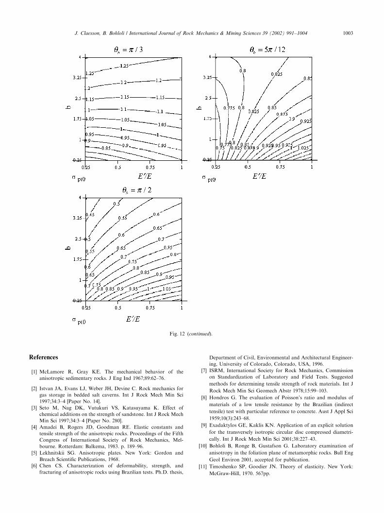
and b; and the angle yb: The scale factor is P=ðpRLÞ:Fig. 12 shows the function spt0ðE0=E; b; ybÞ in charts fordifferent angles yb: Each chart shows the variation of thestress with the parameters E0=E and b for a particularangle yb: The intervals are 0:25pE 0=Ep1 and0:25pbp4; and the angle yb equals np=12; n ¼0; 1;y6: The values for E0=EX1 are obtained fromsymmetry relations (35) with x ¼ y ¼ 0: For all para-meter values

spt0ðE0=E; b; ybÞ ¼ spt0ðE=E0; b; p=2� ybÞ: ð40Þ

Eq. (39) gives the tensile strength of the specimenwhen the scale factor is considered (Fig. 12).

12. Summary and conclusions

The tensile strength of rock is a key parameter thatinfluences rock deformability, rock crushing and blast-ing results. The indirect tensile, or Brazilian, test of rockcores is a common method for determining the tensilestrength. Calculating the tensile strength from theBrazilian test requires knowledge of the principal tensilestress, in particular at the rock core center, where cracksstart. This stress can be assessed by a well-knownanalytical solution for an isotropic material. There existsa much more complicated solution for anisotropic cases,Amadei et al. [4,5]. The calculation of stress and tensilestrength of anisotropic rock sample requires that

the principal elastic constants E; E 0; n; n0 and G0 bedetermined (n=E ¼ n0=E0). This more complicated solu-tion for anisotropic (transversely isotropic) rock wasstudied in detail, which resulted in a few improvementsof the solution method. The convergence of the seriessolution was improved greatly by a new procedure.The stress, strain and displacement can be calculated,even at the disc periphery, with a high degree ofaccuracy without any problems of convergence forthe two opposing normal point loads. The keyexpansion coefficients involve the solution of 4� 4matrix equations. This equation system is reducedto a simpler complex-valued 2� 2 matrix equation(Eq. 25).

The solution is given explicitly. The stress field isobtained by combining Eqs. (5), (6), (10), (13), (14), (16),(19), (21), (22) and (25)–(27). The solution wasimplemented in a mathematical computer program(Mathcad) without any problem. An accuracy of asmany as 5 decimal places is obtained without difficulty.The calculation of the stress field in 10 000 pointsrequires less than 2min of computer time on a goodstandard PC.

The assessment of the analytical solution shows thatthe dimensionless stress field depends only on twointrinsic material parameters (E0=E and b, besides theangle yb between the direction of the applied force andthe normal to the plane of foliation (transverseisotropy). The principal tensile stress at the center of adisc due to opposing normal point loads at the discperiphery may be written in the following dimensionlessform:

sptð0; 0Þ ¼P

pRLspt0ðE0=E; b; ybÞ:

Fig. 11. Principal tensile (left) and compressive (right) stresses in the central area jxj; jyjoR=2 for the reference case, Eq. (29) with yb ¼ p=4:


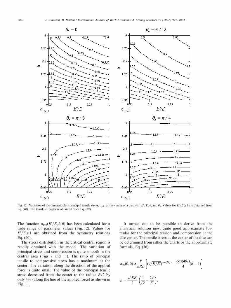
The function spt0ðE0=E; b; yÞ has been calculated for awide range of parameter values (Fig. 12). Values forE0=EX1 are obtained from the symmetry relationsEq. (40).

The stress distribution in the critical central region isreadily obtained with the model. The variation ofprincipal stress and compression is quite smooth in thecentral area (Figs. 7 and 11). The ratio of principaltensile to compressive stress has a maximum at thecenter. The variation along the direction of the appliedforce is quite small. The value of the principal tensilestress decreased from the center to the radius R=2 byonly 4% (along the line of the applied force) as shown inFig. 11.

It turned out to be possible to derive from theanalytical solution new, quite good approximate for-mulas for the principal tension and compression at thedisc center. The tensile stress at the center of the disc canbe determined from either the charts or the approximateformula, Eq. (36):

sptð0; 0ÞDP


pÞcosð2ybÞ �

cosð4ybÞ4

ðb � 1Þ� �

b ¼


p2

1

G0 �2n0

E0

� �:

Fig. 12. Variation of the dimensionless principal tensile stress, spt0; at the center of a disc with E0=E; b; and yb: Values for E0=EZ1 are obtained from

Eq. (40). The tensile strength is obtained from Eq. (39).


References

[1] McLamore R, Gray KE. The mechanical behavior of the

anisotropic sedimentary rocks. J Eng Ind 1967;89:62–76.

[2] Istvan JA, Evans LJ, Weber JH, Devine C. Rock mechanics for

gas storage in bedded salt caverns. Int J Rock Mech Min Sci

1997;34:3–4 [Paper No. 14].

[3] Seto M, Nag DK, Vutukuri VS, Katasuyama K. Effect of

chemical additions on the strength of sandstone. Int J Rock Mech

Min Sci 1997;34:3–4 [Paper No. 280].

[4] Amadei B, Rogers JD, Goodman RE. Elastic constants and

tensile strength of the anisotropic rocks. Proceedings of the Fifth

Congress of International Society of Rock Mechanics, Mel-

bourne. Rotterdam: Balkema, 1983. p. 189–96.

[5] Lekhnitskii SG. Anisotropic plates. New York: Gordon and

Breach Scientific Publications, 1968.

[6] Chen CS. Characterization of deformability, strength, and

fracturing of anisotropic rocks using Brazilian tests. Ph.D. thesis,

Department of Civil, Environmental and Architectural Engineer-

ing, University of Colorado, Colorado, USA, 1996.

[7] ISRM, International Society for Rock Mechanics, Commission

on Standardization of Laboratory and Field Tests. Suggested

methods for determining tensile strength of rock materials. Int J

Rock Mech Min Sci Geomech Abstr 1978;15:99–103.

[8] Hondros G. The evaluation of Poisson’s ratio and modulus of

materials of a low tensile resistance by the Brazilian (indirect

tensile) test with particular reference to concrete. Aust J Appl Sci

1959;10(3):243–68.

[9] Exadaktylos GE, Kaklis KN. Application of an explicit solution

for the transversely isotropic circular disc compressed diametri-

cally. Int J Rock Mech Min Sci 2001;38:227–43.

[10] Bohloli B, Ronge B, Gustafson G. Laboratory examination of

anisotropy in the foliation plane of metamorphic rocks. Bull Eng

Geol Environ 2001, accepted for publication.

[11] Timoshenko SP, Goodier JN. Theory of elasticity. New York:

McGraw-Hill, 1970. 567pp.

Fig. 12 (continued).


[12] Sokolnikoff IS. Mathematical theory of elasticity. New York:

McGraw-Hill, 1956. 476pp.

[13] Muskhelishvili NI. Some basic problems in the mathematical

theory of elasticity. Groningen, The Netherlands: Noordhoff,

1963.

[14] Chen CS, Pan E, Amadei B. Determination of deformability and

tensile strength of anisotropic rock using Brazilian tests. Int J

Rock Mech Min Sci 1998;35(1):43–61.

[15] Amadei B. Importance of anisotropy when estimating and

measuring in-situ stresses in rock. Int J Rock Mech Min Sci

Geomech Abstr 1996;33(3):293–325.

[16] Claesson J. Brazilian test, an analytical solution for a transversely

isotropic disc. Report, Department of Building Physics,

Chalmers University of Technology, Gothenburg, Sweden, 2001.

41pp.

[17] Callen HB. Thermodynamics. New York: Wiley, 1960. 376pp.


Documents

Brazilian test: stress ﬁeld and tensile strength of ...simincoke.co/wp-content/uploads/2017/03/Brazilian test stress field...International Journal of Rock Mechanics & MiningSciences39