Embed Size (px)
DESCRIPTION
It has been claimed by those supporting the hypothesis of anthropogenic global warming (AGW) that ice core measurements prove that levels of carbon dioxide in contemporary air are much greater than prior to the industrial revolution as a result of burning earth-sourced hydrocarbons, more generally known as ‘fossil fuels’. Data from South Pole snow, firn and shallow ice cores demonstrate this premise is unsubstantiated and in fact incorrect. All gas species and isotopes fractionate as they become trapped in the ice sheet and therefore cannot represent absolute concentrations of constituents in historic air.
Citation preview
Breaking Ice Hockey Sticks:
Can Ice be Trusted?
Jonathan J. Drake
8/6/2013
It has been claimed by those supporting the hypothesis of anthropogenic global warming (AGW) that
ice core measurements prove that levels of carbon dioxide in contemporary air are much greater
than prior to the industrial revolution as a result of burning earth-sourced hydrocarbons, more
generally known as ‘fossil fuels’. Data from South Pole snow, firn and shallow ice cores demonstrate
this premise is unsubstantiated and in fact incorrect. All gas species and isotopes fractionate as they
become trapped in the ice sheet and therefore cannot represent absolute concentrations of
constituents in historic air.
Breaking Ice Hockey Sticks: Can Ice be Trusted?
Abstract
It has been claimed by those supporting the hypothesis of anthropogenic global warming (AGW) that
ice core measurements prove that levels of carbon dioxide in contemporary air are much greater
than prior to the industrial revolution as a result of burning earth-sourced hydrocarbons, more
generally known as fossil fuels. The data analysed in this document is from the South Pole and has
been reassessed in various ways. Also, the findings of the authors of the paper that published the
data are highlighted.
The conclusions drawn are that all gaseous species or isotopes undergo fractionation during capture
into the ice sheet. This means that absolute concentrations of trapped air components are not
representative of the atmosphere at the time or close to the time of their capture.
It is also shown that there is divergence between the purported carbon dioxide record and the
modelled oxygen record – based upon fossil fuel usage data – that occurs as the capture process
completes.
Introduction
One of the cornerstones of the Anthropogenic Global Warming hypothesis is the claim that there
was a level of carbon dioxide that was lower and more stable in the so-called pre-industrial times
compared to the contemporary period. The evidence for this is predominantly based upon
concentration measurements of carbon dioxide (CO2), other gas species and isotopes from ice cores,
in particular those from Antarctica. These have become increasingly important as they are claimed
to be almost perfect archives of past atmospheres.
The theory goes that air is trapped in snow as it accumulates on the ground and as the snow
gradually compresses into ice some of the air is integrated into the resultant ice sheet as bubbles.
The bubbles then contain a record of past atmospheric gas concentrations. When the ice is drilled,
cores are collected and the recovered gases are analysed and claimed to accurately represent past
atmospheres.
Those supporting the AGW hypothesis maintain that this entrapment process has no effect on the
carbon dioxide record. To a certain extent, they accept that other gases and isotopes fractionate
during and after capture. Carbon dioxide is claimed to be a special case and as such does not
undergo most of these processes; in particular it does not fractionate relative to the main
atmospheric components during capture.
Is this correct? This document assesses some of the data obtained from shallow depths, at the top
of the ice sheet where snow compresses into ice.
Inspection of the data
The concentrations of a variety of gases have been measured from snow, firn and ice, including
carbon dioxide, at the South Pole, and these will form the principal focus of this assessment. To that
end, reference is made to the paper and data presented by Jeffrey P. Severinghaus & Mark O. Battle,
EPSL 2006: South Pole 2001 and Siple Dome 1996 firn air experiments. This paper will be referred to
as SB2006. Their results for the South Pole ice core are shown as recorded in Figure 1, where the
data is given in relative terms, apart from CO2 which is in absolute concentration.
The lock-in depth or bubble/pore close-off depth is 116m. This is the depth at which the majority of
pores have closed to become bubbles within the ice. It should be clear from this that all the gas
species are displaying relative fractionation, to some extent, both in the snow/firn (above about
116m) and in the ice (below about 116m). The rate of fractionation with depth increases around the
lock-in depth and in some cases reverses.
Why have the SB2006 researchers decided to retain carbon dioxide in absolute concentration (ppm)
whilst all the other gases have been given in per mil relative to a reference (zero depth)? Figure 2
shows the CO2 data normalised in the same way as the other curves but the axis inverted so that it
can be compared to the O2/N2 profile. The reason for comparing CO2 to O2/N2 is simply that they
would be expected to show complimentary trends since O2 is used to create CO2 when hydrocarbons
are burnt in air. Clearly, with this scaling they show a similarity and this will be considered in more
detail later.
All the gases fractionate differently but the two noble gases, Xe and Kr follow similar trends. Ne and
O2 as a pair fractionate in a similar manner, but differently to Xe and Kr. CO2 appears unique within
the set in that it continuously falls with depth whereas all the others tend to increase, but that could
be due to the known contemporary atmospheric increase.
However, the gas species relative concentration fractionation is only part of the story. The South
Pole dataset also contains some isotopic records which are presented in Figure 3. Again, all the
isotopes are displaying fractionation with similar general trends to the gas concentrations and again
there is a distinct change in the relationship with depth at around the bubble close-off.
The change in trends in the region of bubble close-off may suggest that there is more than one
fractionation mechanism is present. This will be discussed later.
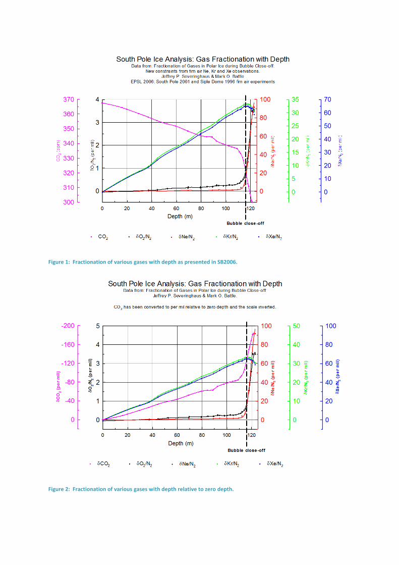
Figure 1: Fractionation of various gases with depth as presented in SB2006.
Figure 2: Fractionation of various gases with depth relative to zero depth.
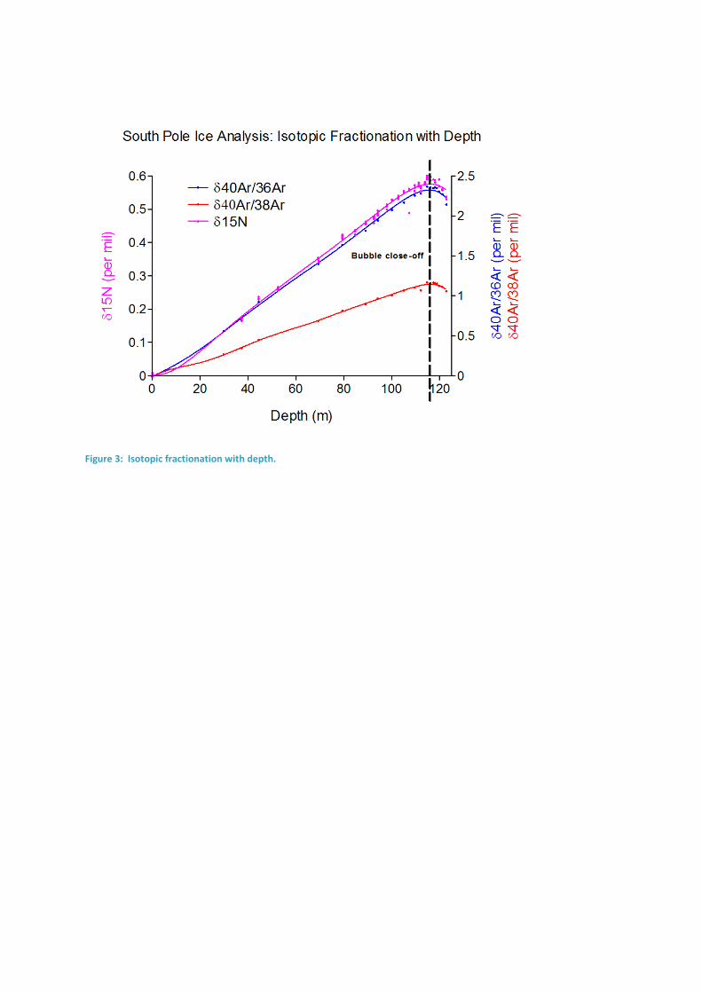
Figure 3: Isotopic fractionation with depth.
At this point, we will move on to looking at the carbon dioxide record in more detail. Of particular
interest is the change in concentration of carbon dioxide with depth and how it is linked to the
assigned chronology. Model data from appendix figures A4 & A6 of SB2006 were used to create a
relationship between sample depth and date. Figure 5 shows the CO2 record using the assigned
dates of the captured gas. The corresponding depths are plotted on the right axis, and the bubble
close-off depth is marked. It is difficult to see any strong semblance between these so a slightly
different approach was taken since there is the possibility of different mechanisms taking place
above and below the bubble close-off depth.
Graphs in Figure 6 & Figure 7 use the same CO2 time series with corresponding depths. They use the
same chronology but focus on different date intervals. As stated earlier, there appears to be
different trends above and below the bubble close-off depth. This depth was used as a break point
estimate for separating the distinct relationships either side. Figure 6 & Figure 7 show there is a
strong similarity between the CO2 concentration and depth profiles on either side of bubble close-
off. This is not immediately obvious if they are considered by looking at the full range of CO2 and
depth as shown in Figure 5. Also, it appears that the relationship alters at a point near to, but not
precisely, the bubble close-off depth and will be referred to as the knee depth.
Note: There is an apparent discontinuity in the data at 1976-1977, the reason for which is not
known and has not been chased down.
For the purposes of the rest of this investigation, a knee depth will be defined as the depth at which
linear function fits to data, above and below the sudden change in fractionation with depth,
intercept. By splitting the data into two, based around the approximate knee depth of 113.2m for
CO2, two linear trends can be fitted. The absolute knee depth designation, as described above, can
have significant uncertainty but it has little effect on the linear fits applied either side of this point.
The linear trend equations were calculated from Figure 8 and yielded these equations:
Y1 = 775.1 - 3.921*X (113m to 125.2m), R2 = 0.9740
Y2 = 369.3 - 0.3004*X (0m to 113m), R2 = 0.9952
It could be argued that a fit other than linear would be more appropriate, which may be true;
however it is irrelevant for the purposes of this study.
From these linear trends, four important points are highlighted. Firstly, the trend of concentration
as a function of depth in the ice, or at least the region examined, limited by the available data, is
about 13 times greater below the knee depth, i.e. in the ice. Secondly, in both regions there is a
reduction in CO2 as the depth increases. Thirdly, the trends either side of knee point are quite linear
with depth, apart from the region of transition. Fourthly, changes in the trends exist for the other
gas species and isotopes presented in SB2006.
Next, if we zoom in on the depth region around bubble close-off, Figure 9, there is a noticeable
difference in the depth at which the trends change; the knee depth in the curves has a spread either
side of the bubble close-off depth. By eye, linear trends were fitted to both sides of the knee for
each gas and the intersection depth determined as the knee depth. A more thorough analysis might
yield slightly different values, but for illustrative purposes the method is adequate.
Table 1 provides the knee depth and a number of physical parameters including kinetic diameter. It
is curious to note that there might be a relationship between the knee depth and kinetic diameter as
shown in Figure 10. However there seems to be stronger relationship between knee depth and
molecular weight as shown in Figure 11. In both these graphs two trends are plotted; one for all the
data (blue) and the other omitting isotopes (cyan).
So what could the reason of the variation in the knee depth? A possible explanation is the reduction
of pore size with increasing depth as can be seen from diffusivity and density plots, Figure 12 &
Figure 13. The mechanisms by which the snow compresses into ice are complex but the resultant
process is well known. Snow falling on the surface builds up and traps a certain amount of air within
its relatively open structure. As more gathers, the lower levels effectively compress and as the
depth increases the more compression takes place. During this process, the voids at low levels are
reduced in size and the air that was originally trapped in them is squeezed and migrates upwards.
As this happens the voids become pores and capillaries develop. Many of these pores and capillaries
are connected with the capillaries providing channels for the pore air to reach the less dense
material above. This the pore and capillary diameters reduce with depth. Due to the need for the
lower air to move out of the lower levels, the bulk of the capillaries provide a pathway upwards to
the surface. Eventually, the pore spaces, and in particular, the capillaries become similar in
diameter to the molecules of air restricting the effective movement. However, due to the varying
sizes, shapes and masses of the gases constituting the air, some will become more constrained than
others at any given depth. As the ice compresses further, there will be a small but significant
upward air motion against which downward diffusion takes place.
At some point, the capillaries become so narrow that the pores effectively close. With further
compression the pressure inside the pore grows and a different diffusion scenario is created. There
is then a pressure imbalance across either a microscopic pore opening or membrane and this can
induce fractionation analogous with membrane separation that is widely used throughout industry.
Molecules escaping from the pressurised pores and bubbles are then exposed to the capillary and
tend to be forced along it, although some upward diffusion will also be present. Any diffusion
downwards is acting against a small but significant largely pressure-induced upward flow.
The result of the compaction process is in effect two fold. Firstly, there is a continuously gradated
molecular sieve above bubble close-off and secondly, at the transition, there is a molecular
membrane sieve that has a differential pressure across it. Thus, it would be expected that as gases
and their isotopes become captured into the ice sheet that significant relative fractionation would
take place. This explains the observed trends with depth and also means that the atmospheric
composition of free air above the ice sheet cannot be preserved within the ice.
However, it should be remembered that the above description has not touched on situations when
the snow melts and refreezes rapidly, in effect instantly creating a thick seal. Generally, that is a rare
occurrence at the South Pole and when it is observed, the data is usually rejected on the basis that
they do not conform to the expected trends.
Above all, it is important to realise that all the processes taking place are driven by climatic
conditions and thus there will be a modulation of the fractionation in response to them.
Furthermore, all the climatic conditions are determined by temperature and so a fairly high level of
coherence between temperature and fractionation of the trapped air is to be expected. Inherently
there will also be a similar degree of correspondence between all the gaseous components.
Indeed it is conceivable that when an atmosphere of constant, uniform composition is subjected to
varying temperature and trapped in ice by this mechanism, under a uniform accumulation rate, the
recovered gas will show little resemblance to the original. The composition will however reflect the
temperature to some degree.
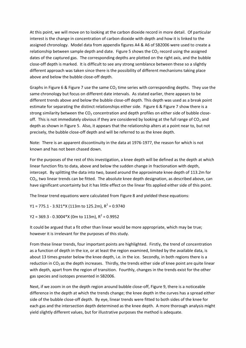
At this juncture, it seems appropriate to mention that glaciologists, or at least some, use the collision
diameter for CO2 of 3.9Å which is rather naïve value to use in such systems. It is essentially an
average size attributed to a linear molecule. The dimension that should be used in this type of
situation is the smallest dimension – critical or kinetic diameter – which for CO2 is around 3.3Å. By
using the collision diameter and comparing it to O2 and N2 it is purported that CO2 does not
fractionate by molecular sieving when air is included in ice sheets because 3.9Å is greater than the
ice lattice gaps estimated to be ~3.6 Å. However, most studies of gas permeability and diffusion
through membranes and porous media, outside of this climate science discipline, use the critical or
kinetic diameter. Figure 4 illustrates some molecular dimensions, but be aware these are not the
same as kinetic diameters, as implied by the name.
Figure 4: Illustration of molecular shapes and dimensions from using molecular simulations for screening of zeolites for separation of CO2/CH4 mixtures. Chemical Engineering Journal, Volume 133, Issues 1–3, 15 September 2007, Pages 121–131.
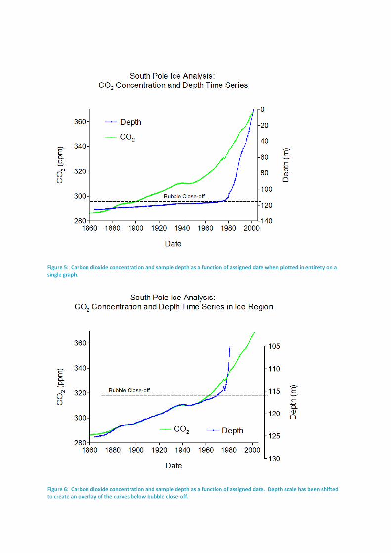
Figure 5: Carbon dioxide concentration and sample depth as a function of assigned date when plotted in entirety on a single graph.
Figure 6: Carbon dioxide concentration and sample depth as a function of assigned date. Depth scale has been shifted to create an overlay of the curves below bubble close-off.
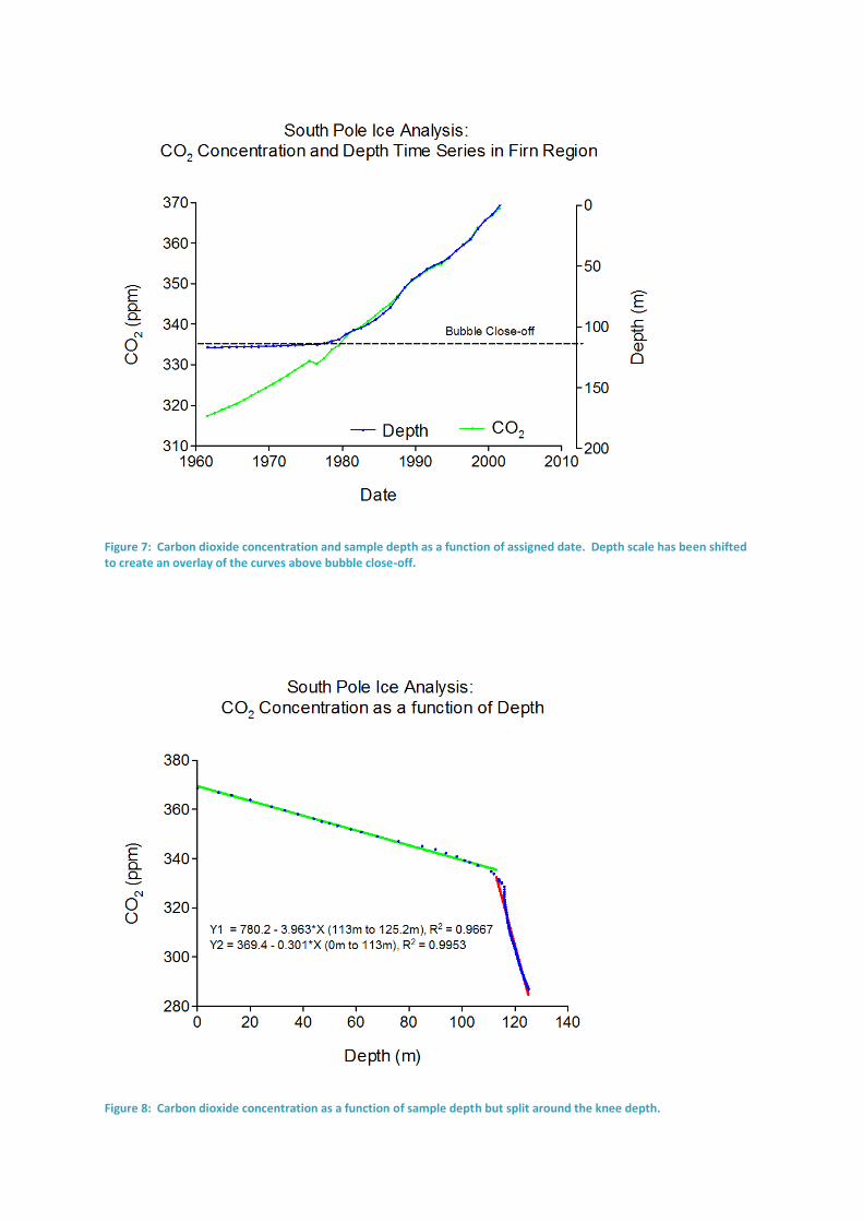
Figure 7: Carbon dioxide concentration and sample depth as a function of assigned date. Depth scale has been shifted to create an overlay of the curves above bubble close-off.
Figure 8: Carbon dioxide concentration as a function of sample depth but split around the knee depth.
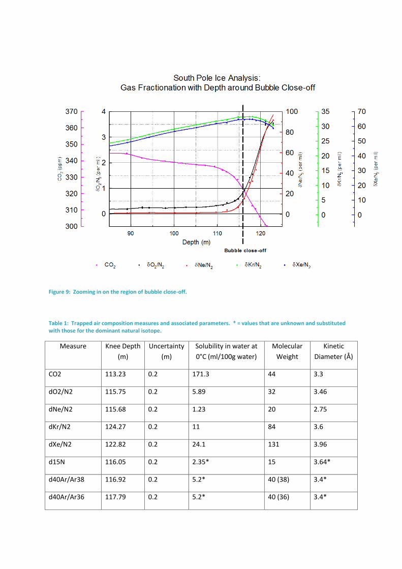
Figure 9: Zooming in on the region of bubble close-off.
Table 1: Trapped air composition measures and associated parameters. * = values that are unknown and substituted with those for the dominant natural isotope.
Measure Knee Depth
(m)
Uncertainty
(m)
Solubility in water at
0°C (ml/100g water)
Molecular
Weight
Kinetic
Diameter (Å)
CO2 113.23 0.2 171.3 44 3.3
dO2/N2 115.75 0.2 5.89 32 3.46
dNe/N2 115.68 0.2 1.23 20 2.75
dKr/N2 124.27 0.2 11 84 3.6
dXe/N2 122.82 0.2 24.1 131 3.96
d15N 116.05 0.2 2.35* 15 3.64*
d40Ar/Ar38 116.92 0.2 5.2* 40 (38) 3.4*
d40Ar/Ar36 117.79 0.2 5.2* 40 (36) 3.4*
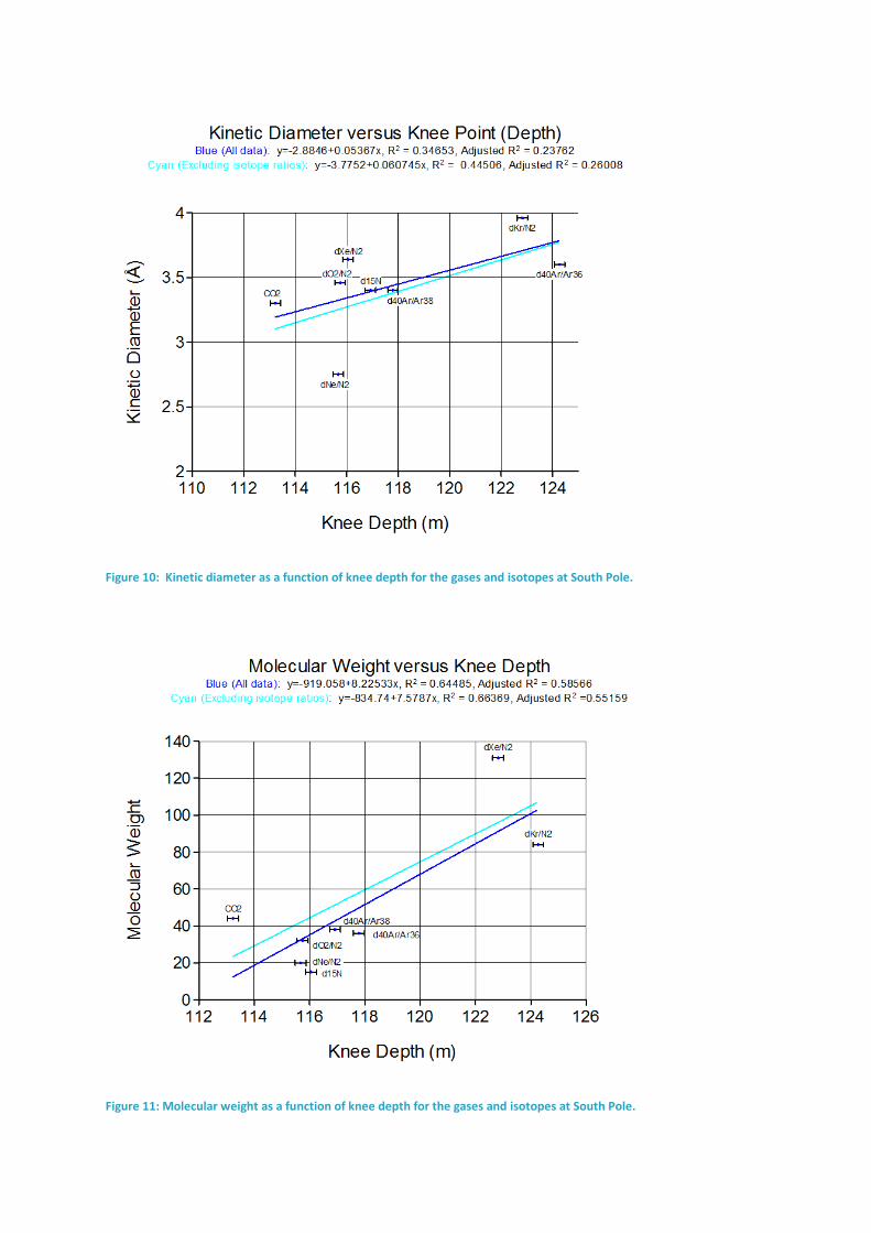
Figure 10: Kinetic diameter as a function of knee depth for the gases and isotopes at South Pole.
Figure 11: Molecular weight as a function of knee depth for the gases and isotopes at South Pole.
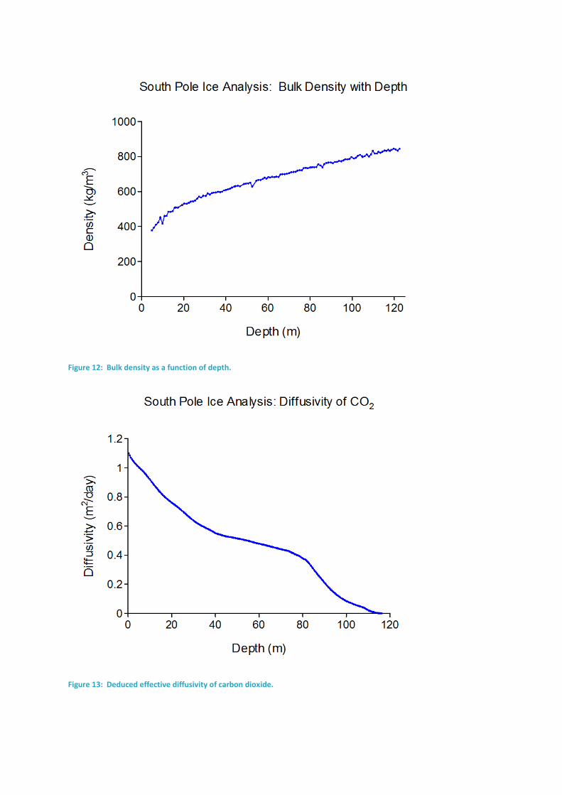
Figure 12: Bulk density as a function of depth.
Figure 13: Deduced effective diffusivity of carbon dioxide.
It is important to remember that the matrix through which filtering and fractionation takes place is
not a constant size and is dynamic. As such it will be difficult, maybe impossible, to model and
correct the data to recover the original atmospheric compositions. At present, the prevailing data
and theoretical mechanism uncertainties will likely mean that potential de-convolution attempts
yield poor results. However, it may be possible to obtain reasonable estimates via empirical
methods, but that will not be considered any further in this document.
Various methods have been used by the glaciologists to match the relatively linear instrumental
record for carbon dioxide with the depth profile in order to create a chronology; mostly correlation.
Not surprisingly, the fairly linear concentration gradient with depth can be readily made to
correspond with the instrumentation record. However, this leads to issues that are glossed over in
most papers but that will be explained here.
Assuming the assigned gas age is correct for CO2 then it should also be largely correct for other
gases. If that is not the case then the composition of the enclosed air cannot be representative of
the original atmosphere. So why are the measured gas concentrations in SB2006 only shown as
depth profiles and not as chronologies? It is easy to find out by creating a depth to time scale using
the data for CO2 and applying it to the other gases. Figure 14 through Figure 17 show the results and
it should be obvious from these that there is a problem with the gas ages being defined by the
carbon dioxide chronology, unless something dramatic happened to the atmosphere around 1980,
which of course is ridiculous.
For the larger noble gas molecules, the reason for the sudden change in concentration around 1980
is clear when considered alongside the deduced effective diffusivity of CO2 and ice density, as shown
in Figure 18 & Figure 19. Simply, they are being fractionated by the ice structure in which they are
restrained.
Another Problem
There are numerous problems in SB2006 when examined in detail; some have been touched on in
this document. However, they are insignificant in comparison to one that is brought to attention
within the paper itself, in the appendix. Here the authors demonstrate that they cannot reconcile
the O2/N2 with the assumed correct CO2 record from ice cores. They find that the O2/N2 data shows
fractionation that is about a factor of 4 greater than ‘expected’. Whilst they show this in a graph – a
copy of which can be seen in Figure 21 – they do not use scales that allow a visual comparison. Since
the data has been made available it is simple to plot it on more suitable scales, Figure 20 which also
provides the depth scale and indications of the close-off and knee depths. As can be seen, the
divergence of the O2/N2 data from the CO2 derived models begins around the depth where the ice
seals the bubbles, about 1980 on the timescale. This is confirmed by image overlay in Figure 22 and
a detail plot of the close-off region is given in Figure 23.
So the O2/N2 and CO2 data are only consistent over a relatively short, approximately linear period
which is coincident with the region above bubble close-off. As has been shown, there is a change in
fractionation at this point due to a transformation in the dynamic physical processes taking place.
The correlation of the matched region should therefore also be considered suspect and more than
likely spurious.
Conclusion
This analysis has shown that fractionation takes place both in the snow/firn and below bubble close-
off in the transition zone/ice for all the observed gases and isotopes. The data provided in SB2006
does not support the assertion that ice is able to trap and retain the composition of ancient or even
contemporary air. This is not particular to the South Pole; it is observed in all locations around the
globe, although the amount and nature of fractionation varies considerably and is dependent upon
local climatic conditions.
Ice core data cannot and should not be considered as a valid archive of past atmospheres, at least
not without correcting for the fractionation that takes place. The United Nations Intergovernmental
Panel on Climate Change relies heavy upon the assertion that the ice core record is infallible,
particularly with regard to a pre-industrial level of carbon dioxide, this document undermines that
cornerstone. Low levels of carbon dioxide in the ice core records are mostly due to fractionation.
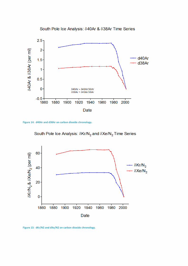
Figure 14: d40Ar and d38Ar on carbon dioxide chronology.
Figure 15: dKr/N2 and dXe/N2 on carbon dioxide chronology.
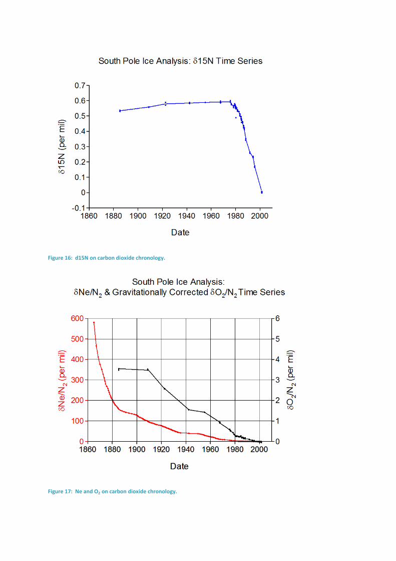
Figure 16: d15N on carbon dioxide chronology.
Figure 17: Ne and O2 on carbon dioxide chronology.
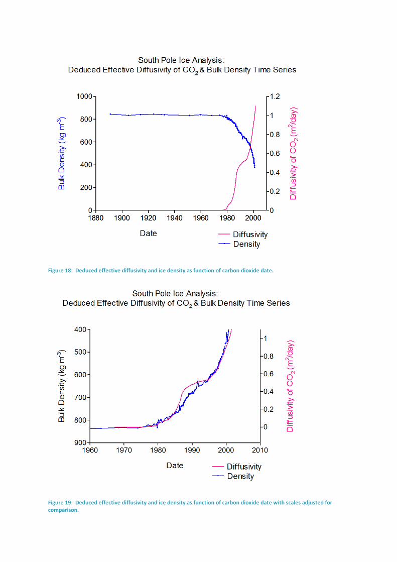
Figure 18: Deduced effective diffusivity and ice density as function of carbon dioxide date.
Figure 19: Deduced effective diffusivity and ice density as function of carbon dioxide date with scales adjusted for comparison.
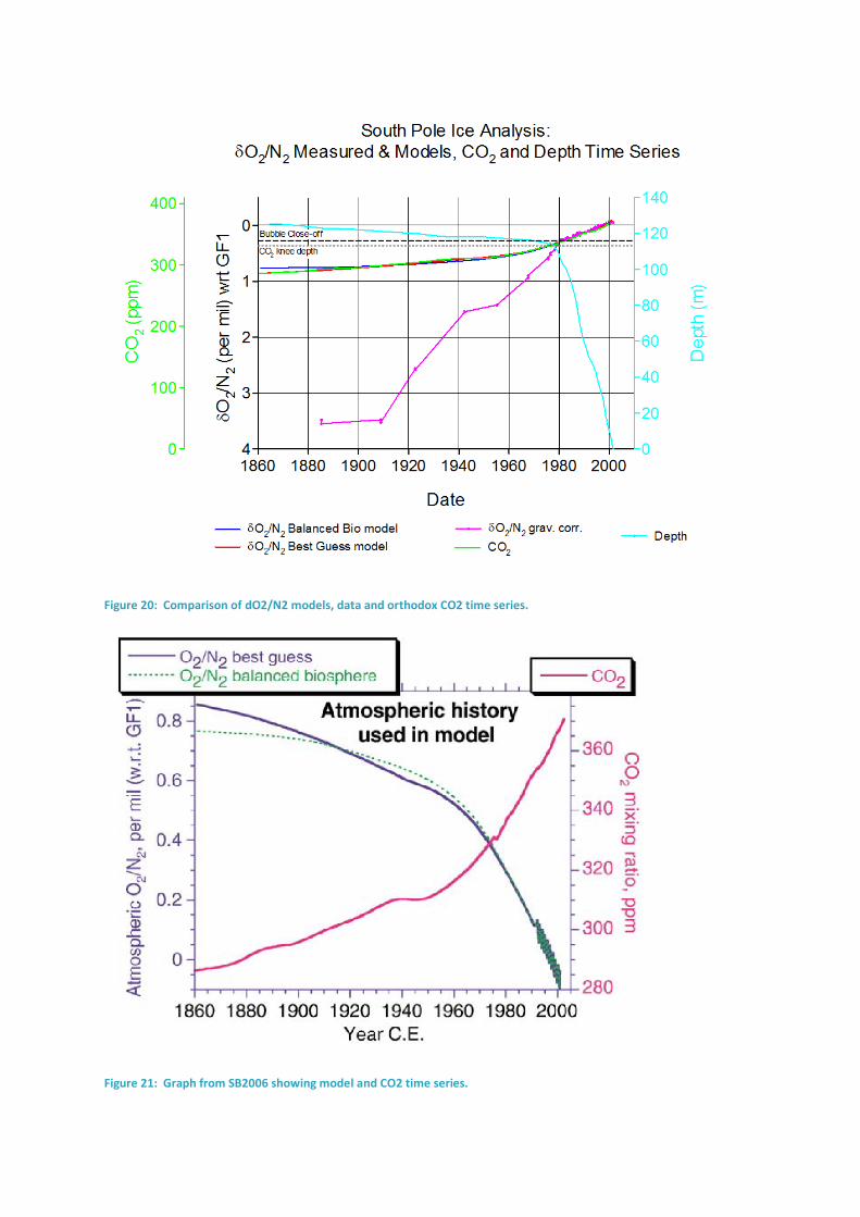
Figure 20: Comparison of dO2/N2 models, data and orthodox CO2 time series.
Figure 21: Graph from SB2006 showing model and CO2 time series.
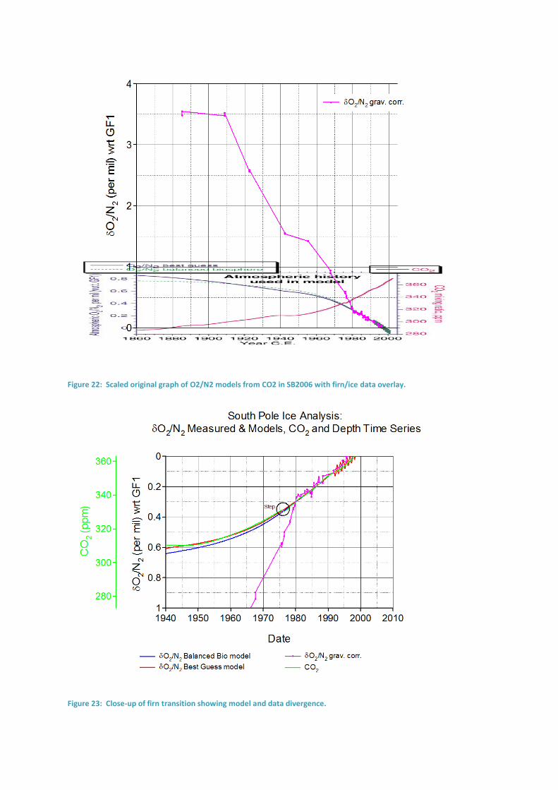
Figure 22: Scaled original graph of O2/N2 models from CO2 in SB2006 with firn/ice data overlay.
Figure 23: Close-up of firn transition showing model and data divergence.
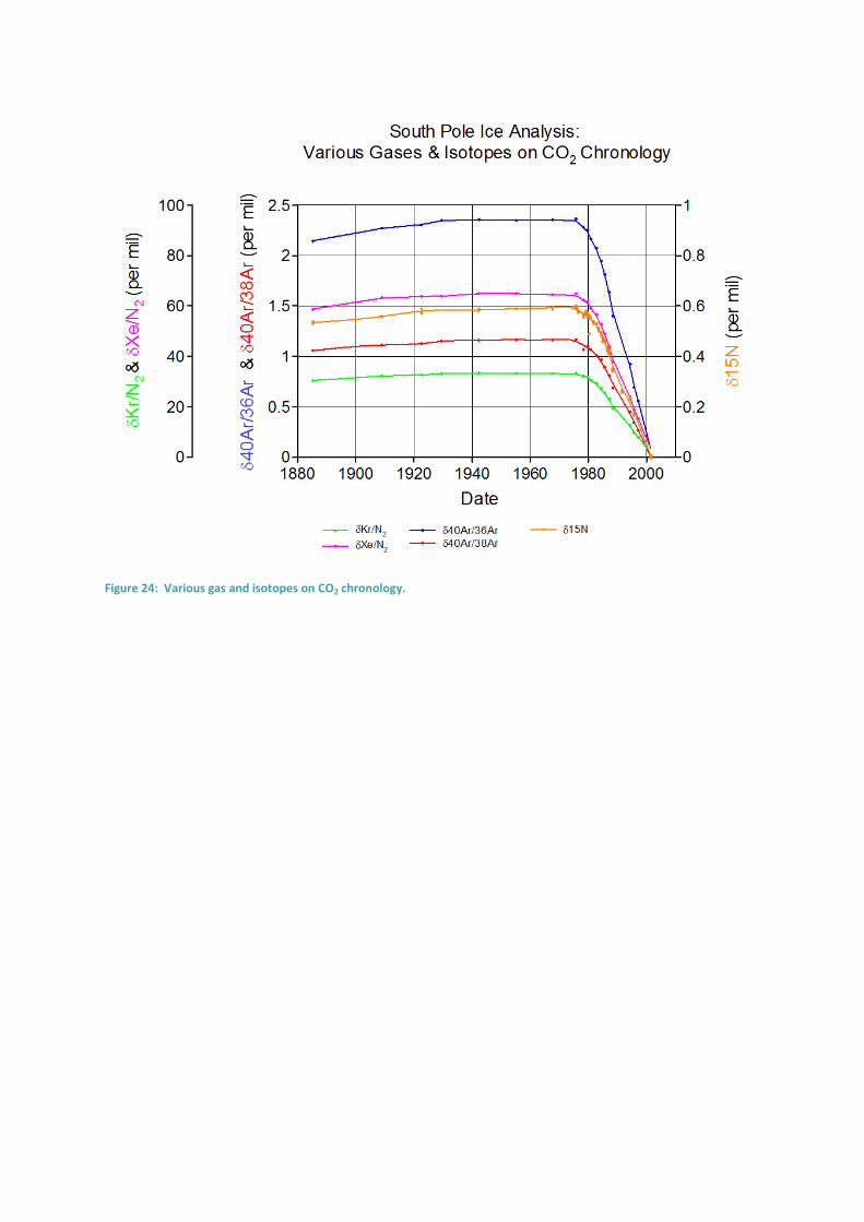
Figure 24: Various gas and isotopes on CO2 chronology.
Bibliography/Reference
1. Michael Bender, Todd Sowers, and Edward Brook: Gases in ice cores. Proc. Natl.
Acad. Sci. USA. Vol. 94, pp. 8343–8349, August 1997.
2. D.W. Breck: Zeolite Molecular Sieves, Structure, Chemistry, and Use, Wiley, New
York, 1974.
3. Christopher J. Cornelius: Physical and Gas Permeation Properties of a Series of Novel
Hybrid Inorganic-Organic Composites Based on a Synthesized Fluorinated Polyimide.
Department of Chemical Engineering, Virginia Polytechnic Institute and State
University, Blacksburg, VA 24061-0211.
4. Colin A. Scholes, Sandra E. Kentish and Geoff W. Stevens: Recent Patents on
Chemical Engineering, 2008, 1, 52-66; 1874-4788/08, 2008. Bentham Science
Publishers Ltd. Carbon Dioxide Separation through Polymeric Membrane Systems
for Flue Gas Applications.
5. Jane R Blackford: Sintering and microstructure of ice: a review. School of
Engineering and Electronics and Centre for Materials Science and Engineering,
Centre for Materials Science and Engineering, University of Edinburgh, EH9 3JL, UK.
J. Phys. D: Appl. Phys. 40 (2007) R355–R385. doi:10.1088/0022-3727/40/21/R02.
6. C. Huber et al: Earth and Planetary Science Letters 243 (2006) 61–73. Evidence for
molecular size dependent gas fractionation in firn air derived from noble gases,
oxygen, and nitrogen measurements.
7. Tomoko Ikeda-Fukazawa et al: Earth and Planetary Science Letters
Volume 229, Issues 3-4, 15 January 2005, Pages 183-192. Effects of molecular
diffusion on trapped gas composition in polar ice cores.
8. Severinghaus, J.P., and Battle, M., Fractionation of gases in polar ice during bubble close-off:
new constraints from firn air Ne, Kr, and Xe observations, Earth Planet Sci. Lett. 244, 474-500
(2006). Link to PDF
9. Using molecular simulations for screening of zeolites for separation of CO2/CH4
mixtures: Chemical Engineering Journal, Volume 133, Issues 1–3, 15 September
2007, Pages 121–131.
http://www.sciencedirect.com/science/article/pii/S1385894707001106
10. Ice Core CO2 Records - Ancient Atmospheres Or Geophysical Artefacts ?
http://robertkernodle.hubpages.com/hub/ICE-Core-CO2-Records-Ancient-
Atmospheres-Or-Geophysical-Artifacts
11.