Embed Size (px)
Citation preview
Brian Howard (#0240783) EE 501, Homework #5 - Manastash Ridge Radar Data Processing
Page 1
To do this project, you will need to download two data files:
http://rrsl.ee.washington.edu/ee501/ref.dat
http://rrsl.ee.washington.edu/ee501/sca.dat
Each of these files represents 10 seconds of IQ data collected on 29 October 2003, UT 10:23:00 with the
radar receivers set to 96.5 MHz. The file ref.dat was collected at the UW, and is an accurate copy of the
FM transmitter signal; the file sca.dat was collected at the Manastash Ridge Radar (near Ellensburg,
WA), and contains the scattered signals.
Problem 1. Data integrity. Load the file ref.dat into your computer analysis tool.
a) Verify that the first four samples are correctly loaded.
In the file ref.dat the first few values are supposed to be:
-5318 first in-phase sample
-771 first quadrature sample
3169 second in-phase sample
-8636 second quadrature sample
Using Matlab I found them to be:
K>> tmp(1:4)
ans =
-5318
-771
3169
-8636
b) Compute the mean and variance of the data. Is the data zero mean? Is it consistent with zero mean?
Using this code:
% Is the data zero mean?
disp(['Mean = ', num2str(mean(abs(data)))]);
ssqn = abs(data).*abs(data);
P1n = sum(ssqn)/N;
Pn = sum(abs(data))/N;
disp(['The signal power for ref.dat is ', num2str(P1n)])
P1varn=(1/sqrt(N))*P1n;
disp(['The expected value for ref.dat is ', num2str(Pn)])
disp(['The variance for ref.dat is ', num2str(std(data)^2)])
disp(['The standard deviation (square root of variance) for ref.dat is ', num2str(std(data))])
Brian Howard (#0240783) EE 501, Homework #5 - Manastash Ridge Radar Data Processing
Page 2
I found:
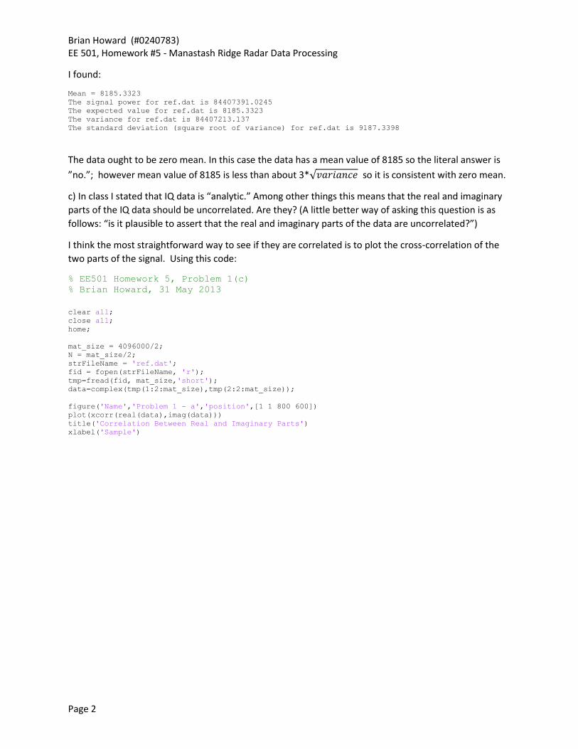
Mean = 8185.3323
The signal power for ref.dat is 84407391.0245
The expected value for ref.dat is 8185.3323
The variance for ref.dat is 84407213.137
The standard deviation (square root of variance) for ref.dat is 9187.3398
The data ought to be zero mean. In this case the data has a mean value of 8185 so the literal answer is
”no.”; however mean value of 8185 is less than about 3*√𝑣𝑎𝑟𝑖𝑎𝑛𝑐𝑒 so it is consistent with zero mean.
c) In class I stated that IQ data is “analytic.” Among other things this means that the real and imaginary
parts of the IQ data should be uncorrelated. Are they? (A little better way of asking this question is as
follows: “is it plausible to assert that the real and imaginary parts of the data are uncorrelated?”)
I think the most straightforward way to see if they are correlated is to plot the cross-correlation of the
two parts of the signal. Using this code:
% EE501 Homework 5, Problem 1(c) % Brian Howard, 31 May 2013
clear all;
close all;
home;
mat_size = 4096000/2;
N = mat_size/2;
strFileName = 'ref.dat';
fid = fopen(strFileName, 'r');
tmp=fread(fid, mat_size,'short');
data=complex(tmp(1:2:mat_size),tmp(2:2:mat_size));
figure('Name','Problem 1 - a','position',[1 1 800 600])
plot(xcorr(real(data),imag(data)))
title('Correlation Between Real and Imaginary Parts')
xlabel('Sample')
Brian Howard (#0240783) EE 501, Homework #5 - Manastash Ridge Radar Data Processing
Page 3
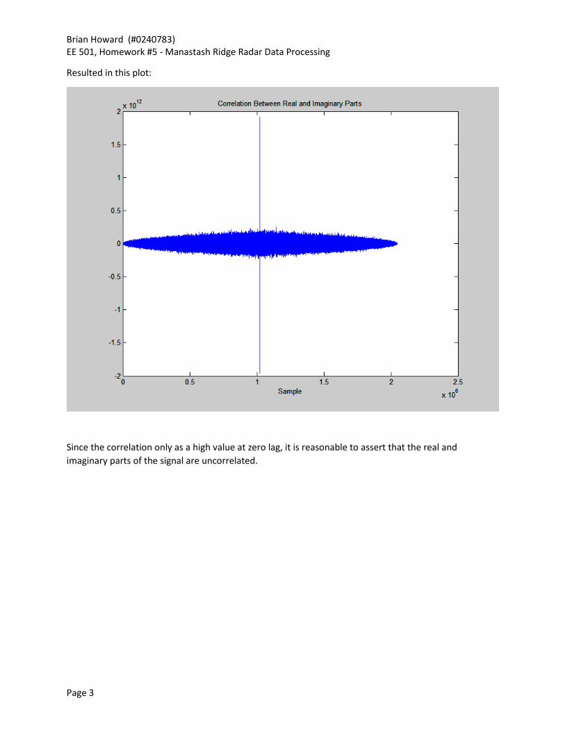
Resulted in this plot:
Since the correlation only as a high value at zero lag, it is reasonable to assert that the real and
imaginary parts of the signal are uncorrelated.
Brian Howard (#0240783) EE 501, Homework #5 - Manastash Ridge Radar Data Processing
Page 4
d) You will be coherently processing the data in chunks of about 0.1 seconds (10,000 samples). Compute
the autocorrelation function R[n] for |n| < 100 and estimate the range resolution. Do this several times,
starting at n = 0, 105, 2 × 10⁵, plotting the magnitude of the autocorrelation |R[n]| for 0 ≤ n ≤ 100.
I used this Matlab code:
% EE501 Homework 5, Problem 1(d)
% Brian Howard, 31 May 2013
clear all;
close all;
home;
mat_size = 4096000/2;
N = mat_size/2;
strFileName = 'ref.dat';
fid = fopen(strFileName, 'r');
tmp=fread(fid, mat_size,'short');
ref=complex(tmp(1:2:mat_size),tmp(2:2:mat_size));
nLag = 100;
figure('Name','Problem 1 - d','position',[1 1 800 600])
iStart = 1;
iEnd = 10000;
data = abs(ref(iStart:iEnd));
data = data - mean(data);
Xc = xcorr(data, nLag);
axLag = -nLag:nLag;
plot(axLag,Xc)
ml = max(Xc)*0.707*ones(size(Xc));
hold on
iStart = iEnd+1;
iEnd = iEnd+10000;
data = abs(ref(iStart:iEnd));
data = data - mean(data);
Xc = xcorr(data, nLag);
plot(axLag,Xc,'g')
iStart = iEnd+1;
iEnd = iEnd+10000;
data = abs(ref(iStart:iEnd));
data = data - mean(data);
Xc = xcorr(data, nLag);
plot(axLag,Xc,'m')
plot(axLag, ml,'r')
legend('1-10000','10001-20000','20001-30000','-3db Line');
title('Autocorrelation |n|<100 (blue) and -3dB Point (Red)')
xlabel('Sample')
Brian Howard (#0240783) EE 501, Homework #5 - Manastash Ridge Radar Data Processing
Page 5
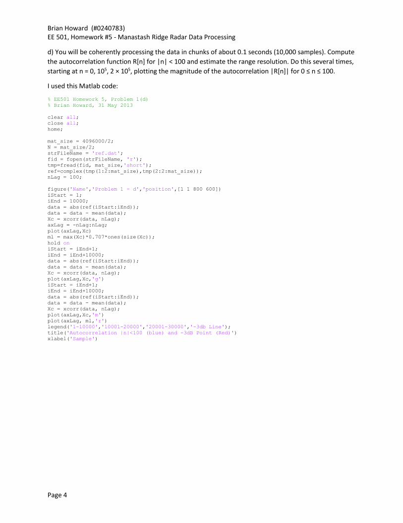
To calculate the autocorrelation:
Treating the autocorrelation like a spectrum I defined the range resolution to be the -3dB width of the
main lobe. In this case the worst case width is ~8 samples or 80µs. This implies a range resolution of
(c/2)* 80µs = 12000 m = 1.2 km.

Brian Howard (#0240783) EE 501, Homework #5 - Manastash Ridge Radar Data Processing
Page 6
e) Make separate histograms of the real part and imaginary part of ref.dat with 50–100 bins. The two
histograms should look pretty similar. Do they? (extra credit: the histograms certainly do *not* appear
gaussian: can you think of why this might be? What do you think that the histograms should look like?
Why?)
Using this code:
% EE501 Homework 5, Problem 1(e)
% Brian Howard, 31 May 2013
clear all;
close all;
home;
mat_size = 4096000/2;
N = mat_size/2;
strFileName = 'ref.dat';
fid = fopen(strFileName, 'r');
tmp=fread(fid, mat_size,'short');
data=complex(tmp(1:2:mat_size),tmp(2:2:mat_size));
figure('Name','Problem 1 - e','position',[1 1 800 600])
subplot(2,1,1)
hist(real(data),100);
title('Histogram of the Real part')
subplot(2,1,2)
hist(imag(data),100);
title('Histogram of the Imaginary part')
Brian Howard (#0240783) EE 501, Homework #5 - Manastash Ridge Radar Data Processing
Page 7
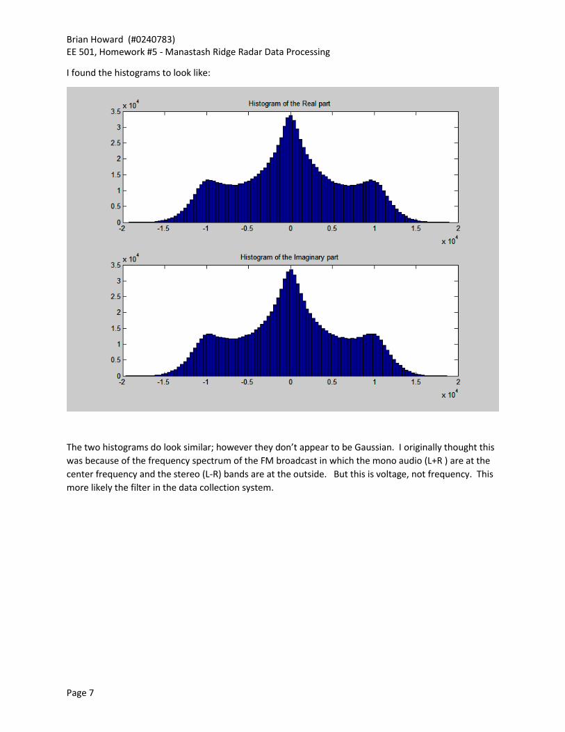
I found the histograms to look like:
The two histograms do look similar; however they don’t appear to be Gaussian. I originally thought this
was because of the frequency spectrum of the FM broadcast in which the mono audio (L+R ) are at the
center frequency and the stereo (L-R) bands are at the outside. But this is voltage, not frequency. This
more likely the filter in the data collection system.
Brian Howard (#0240783) EE 501, Homework #5 - Manastash Ridge Radar Data Processing
Page 8
Problem 2. Data range alignment and rate reduction. In order to do time series analysis for each range,
you will need to combine the two data streams. This can be done several ways, but the following is
straightforward. Define Z(m,r) as follows:
𝑍(𝑚, 𝑟) = ∑ 𝑠𝑐𝑎[𝑚𝐷 + 𝑝 + 𝑟](𝑟𝑒𝑓[𝑚𝐷 + 𝑝])∗𝐷−1
𝑝=0
(1)
This Z(m,r) is an (unbiased) estimate of the signal at range r taken at time mD, thus m is something like
the ”slow time” that we saw for pulsed radars. This Z is effectively the “matched filter detection” of the
target when the transmitter waveform changes constantly, at a rate much faster than the target itself
changes. For this data we expect the full Doppler bandwidth to be less than 2 kHz, so we select D = 50.
This means that Z(m,r) is a 2 kHz time series at range r. We can use Z(m,r) to estimate P1(r) as follows:
�̂�1(𝑟) =1
𝑀∑|𝑍(𝑚, 𝑟)|2𝑀
𝑚=1
(2)
... where M is “as big as possible” given the amount of data available.
a) Write an algorithm to compute Z(m,r). Your algorithm should check to see that m,r,D make sense (lie
within the actual data range). In particular, compute Z(m = 10,r = 42) for D = 50.
I had some trouble with this one. Dr. Sahr gave the values for this m and r as 1011171809-j32362774
which were helpful in correcting my indexing issues. I’m using Matlab so all of my indexes are 1-based
I began by writing a function to calculate Z (it gets used repeatedly in this project):
function [Z] = zcorr(sca, ref, m, r, D)
% function [Z] = zcorr(sca, ref, m, r, D)
%
% INPUT
% sca Complex array with scattered (reciever) data
% ref Complex array of FM transmitter signal
% m Like the "slow time" for pulsed radars. Scalar or vector.
% r Range number. Scalar or vector.
% D Range length. For example, a Doppler bandwidth of 2kHz and
% data sampled at 100kHz implies D = 100000/2000 = 50.
% OUTPUT
% Z This is essentially the correlation between the reference and
% scattered signal. Returns a scalar value if m and r are
% scalars and an array of size (m,r) if m and r are vectors.
% Default value indicating the function failed.
Z = -1000;
N = length(sca);
% check that datasets are the same length
if length(ref)~= N
error('data sets are not the same length');
return;
end
% check that m,r, and D do not exceed array bounds
if( (max(m)*D)>(N-max(r)))
Brian Howard (#0240783) EE 501, Homework #5 - Manastash Ridge Radar Data Processing
Page 9
error('m,r, and D exceed array bounds');
return;
end
% Make the cross-correlation calculation for the case of scalar
if( isequal(size(r),[1 1]) && isequal(size(m),[1 1]) )
Z=0;
mD = (m-1)*D;
Z = Z + dot(sca((mD + (r-1) + 1):(mD + (r-1) + D))',conj(ref( (mD + 1):(mD+D))));
return;
end
% This is the case of r and m vectors
Z = zeros(length(m),length(r));
for ir = 1:length(r)
for im = 1:length(m)
mD = (m(im)-1)*D;
Z(im,ir) = Z(im,ir) + dot(sca((mD + (r(ir)-1) + 1):(mD + (r(ir)-1) + D))',conj(ref( (mD +
1):(mD+D))));
end
end
I then wrote this code to calculate Z at a particular m and r:
% EE501 Homework 5, Problem 2
% Brian Howard, 1 June 2013
clear all;
close all;
home;
mat_size = 4096000/2;
N = mat_size/2;
strFileName = 'ref.dat';
fid = fopen(strFileName, 'r');
tmp=fread(fid, mat_size,'short');
ref=complex(tmp(1:2:mat_size),tmp(2:2:mat_size));
strFileName = 'sca.dat';
fid = fopen(strFileName, 'r');
tmp=fread(fid, mat_size,'short');
sca=complex(tmp(1:2:mat_size),tmp(2:2:mat_size));
D = 50;
Z = zcorr(sca, ref, 11, 43, D)
The code returned:
EDU>> Problem2
Z =
1.0117e+08 - 3.2363e+07i
Which matches pretty well with the values given by the professor.

Brian Howard (#0240783) EE 501, Homework #5 - Manastash Ridge Radar Data Processing
Page 10
b) Use your algorithm to compute �̂�1 for 0 ≤ r ≤ 80. Plot this profile, properly labeling the range axis in
km (assume back scatter geometry).
% EE501 Homework 5, Problem 2(b)
% Brian Howard, 7 June 2013
clear all;
close all;
home;
mat_size = 4096000/2;
N = mat_size/2;
strFileName = 'ref.dat';
fid = fopen(strFileName, 'r');
tmp=fread(fid, mat_size,'short');
ref=complex(tmp(1:2:mat_size),tmp(2:2:mat_size));
strFileName = 'sca.dat';
fid = fopen(strFileName, 'r');
tmp=fread(fid, mat_size,'short');
sca=complex(tmp(1:2:mat_size),tmp(2:2:mat_size));
D = 50;
fs = 100000;
c = 300000000;
% Only need to run these lines once. Just load it otherwise
if 1
r = 1:81;
m = 1:(fix((N-max(r))/D));
Z = zcorr(sca, ref, m, r, D);
save('Z80.mat','Z');
end
load('Z80');
% calculate the power estimate
M = min(size(Z));
Pest = zeros(M,1);
for r = 1:M
P(r) = dot(Z(:,r),Z(:,r));
P(r) = P(r)./M;
end
% calculate the range in km
rd = (0:(M-1)).*(1/fs)*(c/2)*0.001;
% plot the data
figure('Name','Problem 2 - b','position',[1 1 800 600])
plot(rd,P)
title('Estimated Power');
xlabel('Distance, km');
Brian Howard (#0240783) EE 501, Homework #5 - Manastash Ridge Radar Data Processing
Page 11
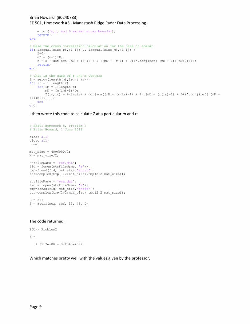
Resulted in this plot:
I’m guessing that big peak is Rainer?

Brian Howard (#0240783) EE 501, Homework #5 - Manastash Ridge Radar Data Processing
Page 12
c) What is the range resolution? (and what do you mean by ”range resolution”?)
In this problem the smallest distance in time that we can discriminate is 1/sampling frequency. For this
project that works out to a time of 0.01ms. Since we are assuming backscatter geometry, this time
interval works out to a distance of 1.5km of range resolution.
d) What is the range of the Doppler velocities that can be expressed in the time series Z(m,r) at a
particular fixed range r?
Doppler velocity equals (fd*λ)/2. The Doppler frequency is 2kHz (since D=50) and λ is 3.1m so that the
velocity range is 3100m/s or +/-1550m/s.

Brian Howard (#0240783) EE 501, Homework #5 - Manastash Ridge Radar Data Processing
Page 13
Problem 3. Spectrum Estimation. Setting D = 50 and r = 42 (or matlab range 43), compute and plot the
power spectrum as indicated below.
a) How many samples Z(m,42) are available?
Using the size of the file and the parameters given in the problem I calculate the number of samples as:
mat_size = 4096000/2;
N = mat_size/2;
D = 50;
r = 43;
m = (fix((N-max(r))/D))
This gives the result of:
m = 20479
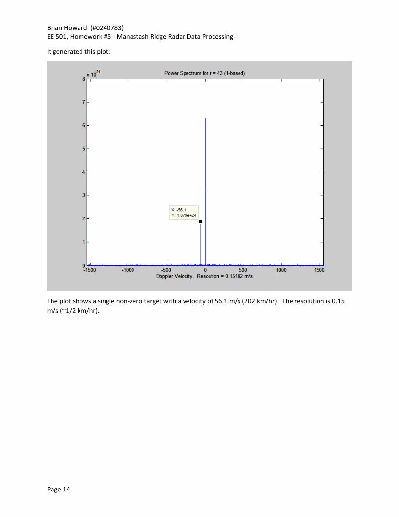
b) Plot abs(FFT(Z(:,42))).^2. Do you see any (nonzero Doppler velocity) target? What is its velocity?
What is the Doppler Velocity resolution?
This is the code I used:
% EE501 Homework 5, Problem 3
% Brian Howard, 8 June 2013
clear all;
close all;
home;
c = 300000000;
fb = 96500000;
lambda = c/fb;
D = 50;
fs = 100000;
load('Z80');
r = 43;
Y = fftshift(abs(fft(Z(:,r))).^2);
n = length(Y);
fd = (fs/(2*D))*lambda/2;
fds =((-(n-1)/2):((n-1)/2))./((n-1)/2);
fds = fds.*fd;
figure('Name','Problem 3 - b','position',[1 1 800 600])
plot(fds,Y);
title(['Power Spectrum for r = ' num2str(r) ' (1-based)'])
xlabel(['Doppler Velocity. Resoution = ' num2str(fds(2)-fds(1)) ' m/s']);
xlim([min(fds) max(fds)]);
Brian Howard (#0240783) EE 501, Homework #5 - Manastash Ridge Radar Data Processing
Page 14
It generated this plot:
The plot shows a single non-zero target with a velocity of 56.1 m/s (202 km/hr). The resolution is 0.15
m/s (~1/2 km/hr).
Brian Howard (#0240783) EE 501, Homework #5 - Manastash Ridge Radar Data Processing
Page 15
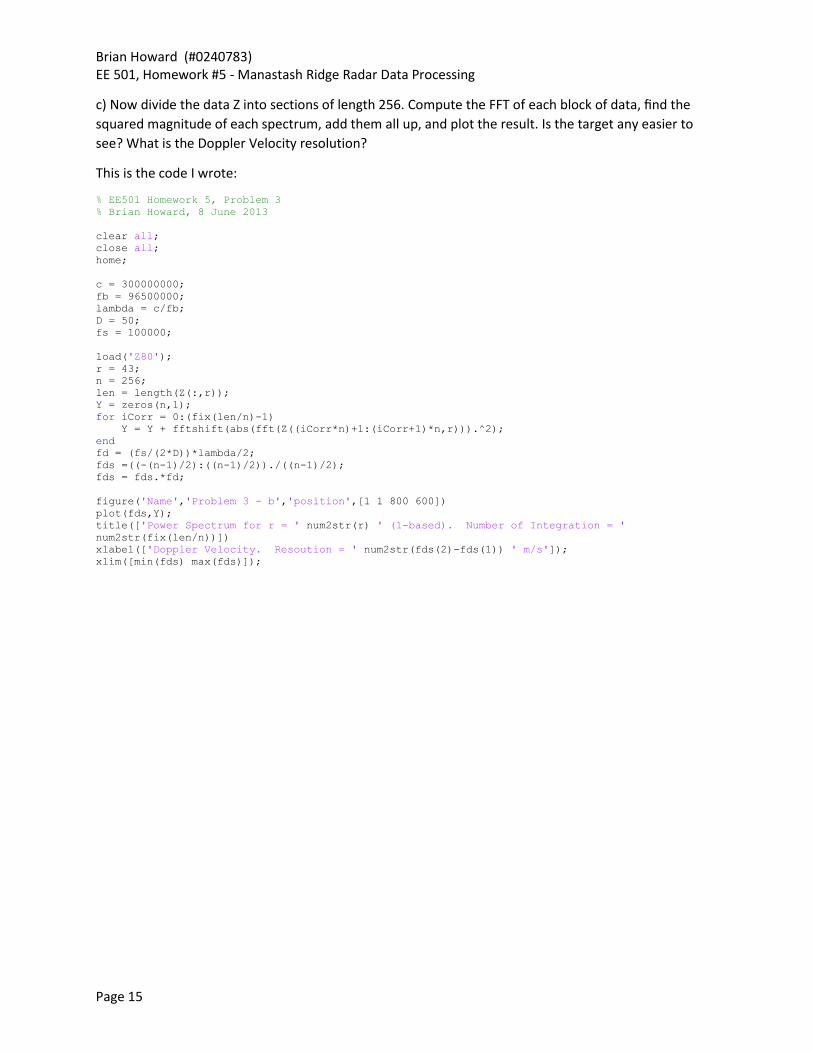
c) Now divide the data Z into sections of length 256. Compute the FFT of each block of data, find the
squared magnitude of each spectrum, add them all up, and plot the result. Is the target any easier to
see? What is the Doppler Velocity resolution?
This is the code I wrote:
% EE501 Homework 5, Problem 3
% Brian Howard, 8 June 2013
clear all;
close all;
home;
c = 300000000;
fb = 96500000;
lambda = c/fb;
D = 50;
fs = 100000;
load('Z80');
r = 43;
n = 256;
len = length(Z(:,r));
Y = zeros(n,1);
for iCorr = 0:(fix(len/n)-1)
Y = Y + fftshift(abs(fft(Z((iCorr*n)+1:(iCorr+1)*n,r))).^2);
end
fd = (fs/(2*D))*lambda/2;
fds =((-(n-1)/2):((n-1)/2))./((n-1)/2);
fds = fds.*fd;
figure('Name','Problem 3 - b','position',[1 1 800 600])
plot(fds,Y);
title(['Power Spectrum for r = ' num2str(r) ' (1-based). Number of Integration = '
num2str(fix(len/n))])
xlabel(['Doppler Velocity. Resoution = ' num2str(fds(2)-fds(1)) ' m/s']);
xlim([min(fds) max(fds)]);

Brian Howard (#0240783) EE 501, Homework #5 - Manastash Ridge Radar Data Processing
Page 16
It resulted in this figure:
The target appears much easier to see, especially with respect to the ground clutter, but Doppler
resolution has increased from 0.15 m/s to 12.2 m/s due to the lower bin count in the FFT.
Brian Howard (#0240783) EE 501, Homework #5 - Manastash Ridge Radar Data Processing
Page 17
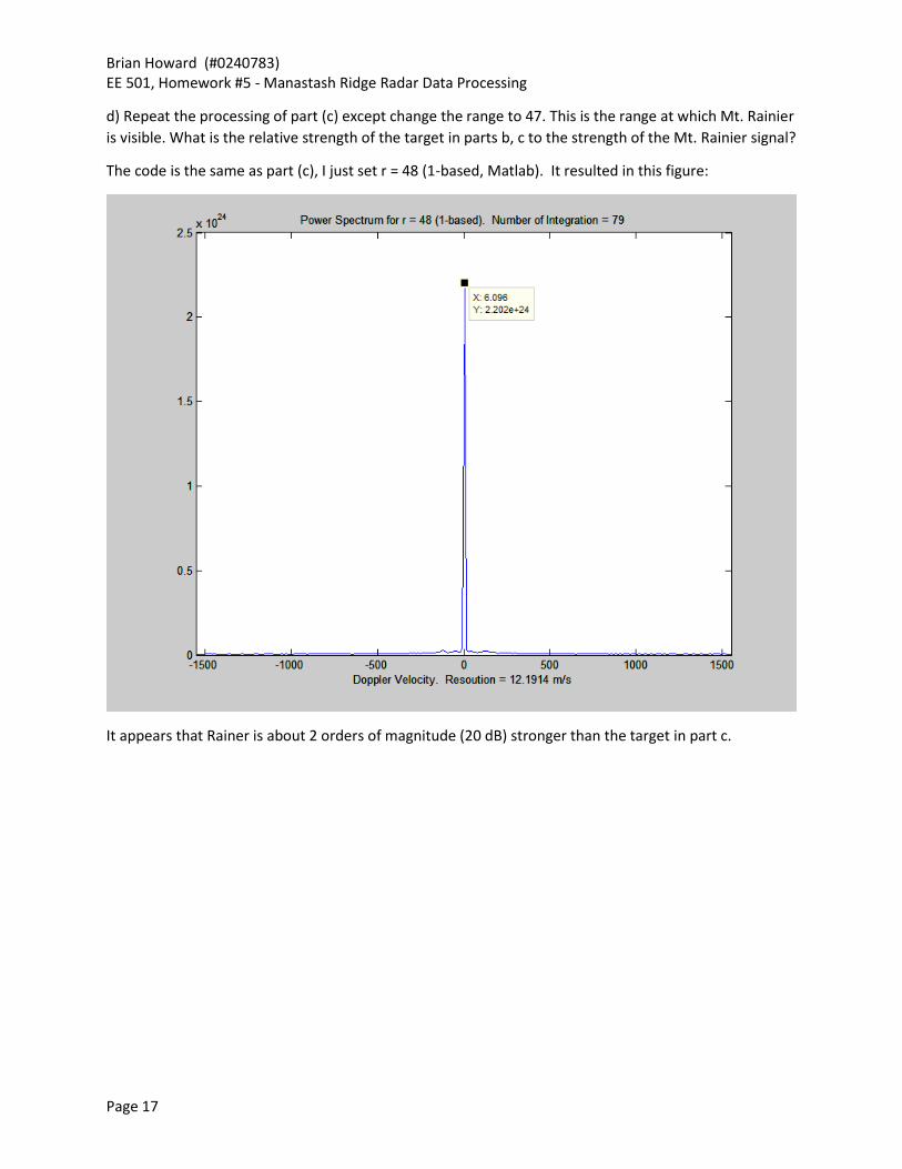
d) Repeat the processing of part (c) except change the range to 47. This is the range at which Mt. Rainier
is visible. What is the relative strength of the target in parts b, c to the strength of the Mt. Rainier signal?
The code is the same as part (c), I just set r = 48 (1-based, Matlab). It resulted in this figure:
It appears that Rainer is about 2 orders of magnitude (20 dB) stronger than the target in part c.
Brian Howard (#0240783) EE 501, Homework #5 - Manastash Ridge Radar Data Processing
Page 18
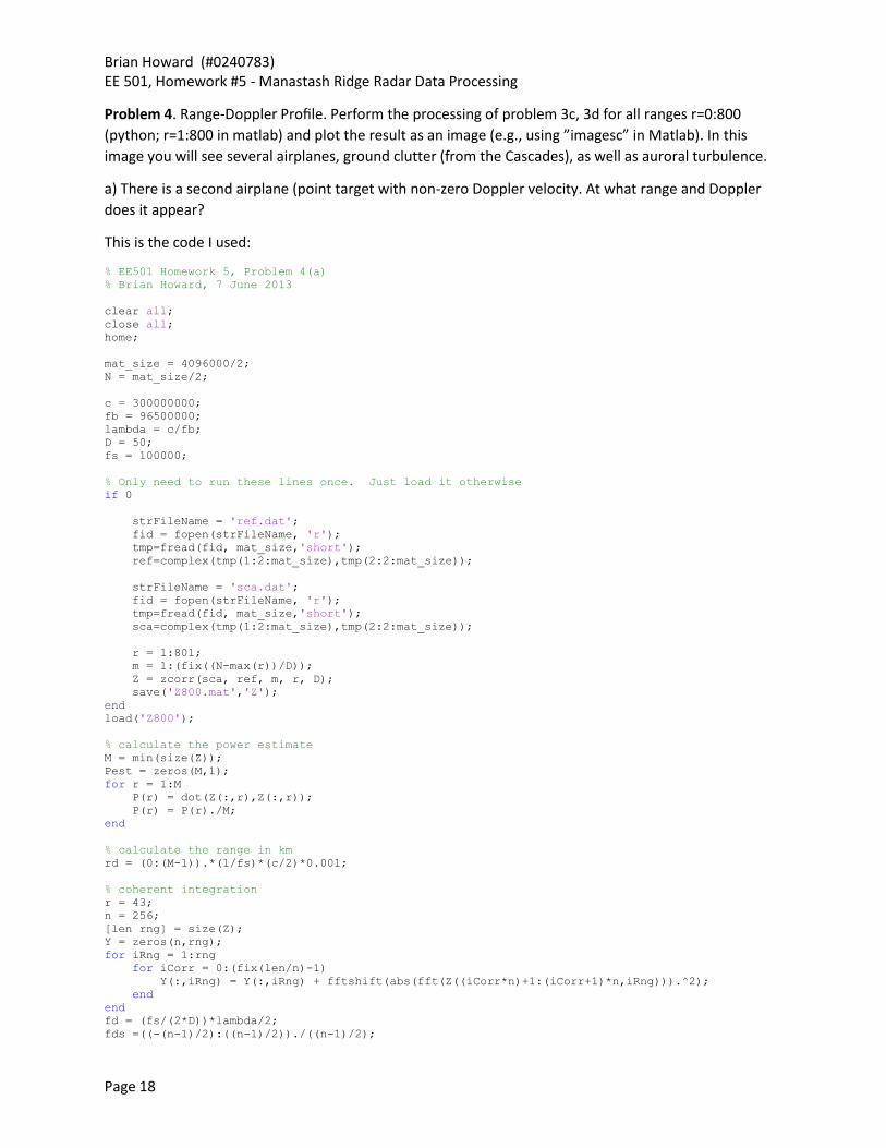
Problem 4. Range-Doppler Profile. Perform the processing of problem 3c, 3d for all ranges r=0:800
(python; r=1:800 in matlab) and plot the result as an image (e.g., using ”imagesc” in Matlab). In this
image you will see several airplanes, ground clutter (from the Cascades), as well as auroral turbulence.
a) There is a second airplane (point target with non-zero Doppler velocity. At what range and Doppler
does it appear?
This is the code I used:
% EE501 Homework 5, Problem 4(a)
% Brian Howard, 7 June 2013
clear all;
close all;
home;
mat_size = 4096000/2;
N = mat_size/2;
c = 300000000;
fb = 96500000;
lambda = c/fb;
D = 50;
fs = 100000;
% Only need to run these lines once. Just load it otherwise
if 0
strFileName = 'ref.dat';
fid = fopen(strFileName, 'r');
tmp=fread(fid, mat_size,'short');
ref=complex(tmp(1:2:mat_size),tmp(2:2:mat_size));
strFileName = 'sca.dat';
fid = fopen(strFileName, 'r');
tmp=fread(fid, mat_size,'short');
sca=complex(tmp(1:2:mat_size),tmp(2:2:mat_size));
r = 1:801;
m = 1:(fix((N-max(r))/D));
Z = zcorr(sca, ref, m, r, D);
save('Z800.mat','Z');
end
load('Z800');
% calculate the power estimate
M = min(size(Z));
Pest = zeros(M,1);
for r = 1:M
P(r) = dot(Z(:,r),Z(:,r));
P(r) = P(r)./M;
end
% calculate the range in km
rd = (0:(M-1)).*(1/fs)*(c/2)*0.001;
% coherent integration
r = 43;
n = 256;
[len rng] = size(Z);
Y = zeros(n,rng);
for iRng = 1:rng
for iCorr = 0:(fix(len/n)-1)
Y(:,iRng) = Y(:,iRng) + fftshift(abs(fft(Z((iCorr*n)+1:(iCorr+1)*n,iRng))).^2);
end
end
fd = (fs/(2*D))*lambda/2;
fds =((-(n-1)/2):((n-1)/2))./((n-1)/2);
Brian Howard (#0240783) EE 501, Homework #5 - Manastash Ridge Radar Data Processing
Page 19
fds = fds.*fd;
figure('Name','Problem 4 - a','position',[1 1 800 600])
plot(fds,Y(:,r));
title(['Power Spectrum for r = ' num2str(r) ' (1-based). Number of Integration = '
num2str(fix(len/n))])
xlabel(['Doppler Velocity. Resoution = ' num2str(fds(2)-fds(1)) ' m/s']);
xlim([min(fds) max(fds)]);
% plot the data
figure('Name','Problem 4 - a','position',[1 1 800 600])
imagesc([min(fds) max(fds)], [1 max(rd)], (log10(Y)'))
title(['Log of Power Spectrum. Number of Integration = ' num2str(fix(len/n))])
xlabel(['Doppler Velocity. Resoution = ' num2str(fds(2)-fds(1)) ' m/s']);
ylabel('Distance, km');
set(gca,'YDir','normal')
caxis([21.5 24])
colorbar
figure('Name','Problem 4 - a','position',[1 1 800 600])
hSurf = surf((log10(Y)'),'EdgeColor','none','LineStyle','none','FaceColor','interp');
camproj('orthographic')
set(gca,'YDir','normal')
caxis([21.5 24])
view([-31.5 24]);
colorbar
Brian Howard (#0240783) EE 501, Homework #5 - Manastash Ridge Radar Data Processing
Page 20
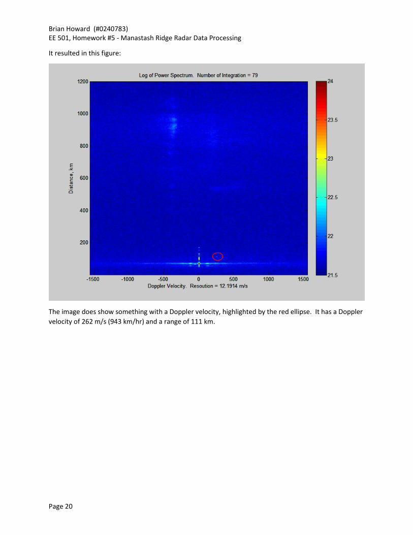
It resulted in this figure:
The image does show something with a Doppler velocity, highlighted by the red ellipse. It has a Doppler
velocity of 262 m/s (943 km/hr) and a range of 111 km.

Brian Howard (#0240783) EE 501, Homework #5 - Manastash Ridge Radar Data Processing
Page 21
b) Most of the range-Doppler image contains no scattered signal; we call this the ”clutter floor.” What is
the strength of the clutter floor? How strong is the Mt. Rainier echo compared to the clutter floor (in
dB)? How strong are the two airplane echoes compared to the clutter floor?
Referring to the plot, which shows the log10 of the power spectrum and should be reading in decibels,
the clutter floor strength is about 21.5 and Mt Rainier is about 24, a 3.5 dB difference. The airplanes are
about 23 and 22, or 1-2 dB above the clutter floor.
c) At what ranges do you see Auroral Turbulence?
It looks to start around 500 km and extend upward to about 1000 km.
d) Auroral turbulence occurs at an altitude of 110 km, and certainly occurs far beyond the 800 ranges
(1200 km). Why is it pointless to look for auroral echoes further than 800 ranges?
The turbulence is at a constant elevation, but larger ranges are echoes from further away. As the
distance increases the curvature of the earth begins to block the signal. In short, it is the Canadians
fault, their country gets in the way.
Brian Howard (#0240783) EE 501, Homework #5 - Manastash Ridge Radar Data Processing
Page 22
Problem 5. Reduced Precision.
a) Take the original data and divide each by 5000 and round to the nearest integer; this simulates use of
a 4 bit digitizer. Form the range-Doppler image using this truncated data, and compare it to your image
from problem 3.
Using this code:
% EE501 Homework 5, Problem 5(a)
% Brian Howard, 7 June 2013
clear all;
close all;
home;
mat_size = 4096000/2;
N = mat_size/2;
c = 300000000;
fb = 96500000;
lambda = c/fb;
D = 50;
fs = 100000;
% Only need to run these lines once. Just load it otherwise
if 0
strFileName = 'ref.dat';
fid = fopen(strFileName, 'r');
tmp=fread(fid, mat_size,'short');
tmp=fix(tmp./5000);
ref=complex(tmp(1:2:mat_size),tmp(2:2:mat_size));
strFileName = 'sca.dat';
fid = fopen(strFileName, 'r');
tmp=fread(fid, mat_size,'short');
tmp=fix(tmp./5000);
sca=complex(tmp(1:2:mat_size),tmp(2:2:mat_size));
r = 1:801;
m = 1:(fix((N-max(r))/D));
Z = zcorr(sca, ref, m, r, D);
save('Z800ds.mat','Z');
end
load('Z800ds');
% calculate the power estimate
M = min(size(Z));
Pest = zeros(M,1);
for r = 1:M
P(r) = dot(Z(:,r),Z(:,r));
P(r) = P(r)./M;
end
% calculate the range in km
rd = (0:(M-1)).*(1/fs)*(c/2)*0.001;
% coherent integration
r = 43;
n = 256;
[len rng] = size(Z);
Y = zeros(n,rng);
for iRng = 1:rng
for iCorr = 0:(fix(len/n)-1)
Y(:,iRng) = Y(:,iRng) + fftshift(abs(fft(Z((iCorr*n)+1:(iCorr+1)*n,iRng))).^2);
end
end
fd = (fs/(2*D))*lambda/2;
Brian Howard (#0240783) EE 501, Homework #5 - Manastash Ridge Radar Data Processing
Page 23
fds =((-(n-1)/2):((n-1)/2))./((n-1)/2);
fds = fds.*fd;
figure('Name','Problem 5 - a','position',[1 1 800 600])
plot(fds,Y(:,r));
title(['Power Spectrum for r = ' num2str(r) ' (1-based). Number of Integration = '
num2str(fix(len/n))])
xlabel(['Doppler Velocity. Resoution = ' num2str(fds(2)-fds(1)) ' m/s']);
xlim([min(fds) max(fds)]);
% plot the data
figure('Name','Problem 5 - a','position',[1 1 800 600])
imagesc([min(fds) max(fds)], [1 max(rd)], (log10(Y)'))
title(['Log of Power Spectrum (Reduced Precision). Number of Integration = '
num2str(fix(len/n))])
xlabel(['Doppler Velocity. Resoution = ' num2str(fds(2)-fds(1)) ' m/s']);
ylabel('Distance, km');
set(gca,'YDir','normal')
%caxis([21.5 24])
colorbar
figure('Name','Problem 5 - a','position',[1 1 800 600])
hSurf = surf((log10(Y)'),'EdgeColor','none','LineStyle','none','FaceColor','interp');
camproj('orthographic')
set(gca,'YDir','normal')
%caxis([21.5 24])
view([-31.5 24]);
colorbar

Brian Howard (#0240783) EE 501, Homework #5 - Manastash Ridge Radar Data Processing
Page 24
Resulted in this plot:
It looks pretty good, not so different from the higher precision images above.

Brian Howard (#0240783) EE 501, Homework #5 - Manastash Ridge Radar Data Processing
Page 25
b) Take the original data and reduce it to the sign bit only (in each of the real and imaginary parts); that
is, the only possible data points are ±1 ± j. Form the range-Doppler image using this truncated data, and
compare it to your image from problem 3.
% EE501 Homework 5, Problem 5(b)
% Brian Howard, 7 June 2013
clear all;
close all;
home;
mat_size = 4096000/2;
N = mat_size/2;
c = 300000000;
fb = 96500000;
lambda = c/fb;
D = 50;
fs = 100000;
% Only need to run these lines once. Just load it otherwise
if 1
strFileName = 'ref.dat';
fid = fopen(strFileName, 'r');
tmp=fread(fid, mat_size,'short');
tmp=sign(tmp);
ref=complex(tmp(1:2:mat_size),tmp(2:2:mat_size));
strFileName = 'sca.dat';
fid = fopen(strFileName, 'r');
tmp=fread(fid, mat_size,'short');
tmp=sign(tmp);
sca=complex(tmp(1:2:mat_size),tmp(2:2:mat_size));
r = 1:801;
m = 1:(fix((N-max(r))/D));
Z = zcorr(sca, ref, m, r, D);
save('Z800ds.mat','Z');
end
load('Z800ds');
% calculate the power estimate
M = min(size(Z));
Pest = zeros(M,1);
for r = 1:M
P(r) = dot(Z(:,r),Z(:,r));
P(r) = P(r)./M;
end
% calculate the range in km
rd = (0:(M-1)).*(1/fs)*(c/2)*0.001;
% coherent integration
r = 43;
n = 256;
[len rng] = size(Z);
Y = zeros(n,rng);
for iRng = 1:rng
for iCorr = 0:(fix(len/n)-1)
Y(:,iRng) = Y(:,iRng) + fftshift(abs(fft(Z((iCorr*n)+1:(iCorr+1)*n,iRng))).^2);
end
end
fd = (fs/(2*D))*lambda/2;
fds =((-(n-1)/2):((n-1)/2))./((n-1)/2);
fds = fds.*fd;
figure('Name','Problem 5 - b','position',[1 1 800 600])
plot(fds,Y(:,r));
Brian Howard (#0240783) EE 501, Homework #5 - Manastash Ridge Radar Data Processing
Page 26
title(['Power Spectrum for r = ' num2str(r) ' (1-based). Number of Integration = '
num2str(fix(len/n))])
xlabel(['Doppler Velocity. Resoution = ' num2str(fds(2)-fds(1)) ' m/s']);
xlim([min(fds) max(fds)]);
% plot the data
figure('Name','Problem 5 - b','position',[1 1 800 600])
imagesc([min(fds) max(fds)], [1 max(rd)], (log10(Y)'))
title(['Log of Power Spectrum (1-Bit Precision). Number of Integration = ' num2str(fix(len/n))])
xlabel(['Doppler Velocity. Resoution = ' num2str(fds(2)-fds(1)) ' m/s']);
ylabel('Distance, km');
set(gca,'YDir','normal')
%caxis([21.5 24])
colorbar
figure('Name','Problem 5 - b','position',[1 1 800 600])
hSurf = surf((log10(Y)'),'EdgeColor','none','LineStyle','none','FaceColor','interp');
camproj('orthographic')
set(gca,'YDir','normal')
%caxis([21.5 24])
view([-31.5 24]);
colorbar

Brian Howard (#0240783) EE 501, Homework #5 - Manastash Ridge Radar Data Processing
Page 27
It resulted in this figure:
Not bad at all!!! It is a little harder to see the turbulence, which might be a problem if the data is being
used to quantify behavior there.
Brian Howard (#0240783) EE 501, Homework #5 - Manastash Ridge Radar Data Processing
Page 28
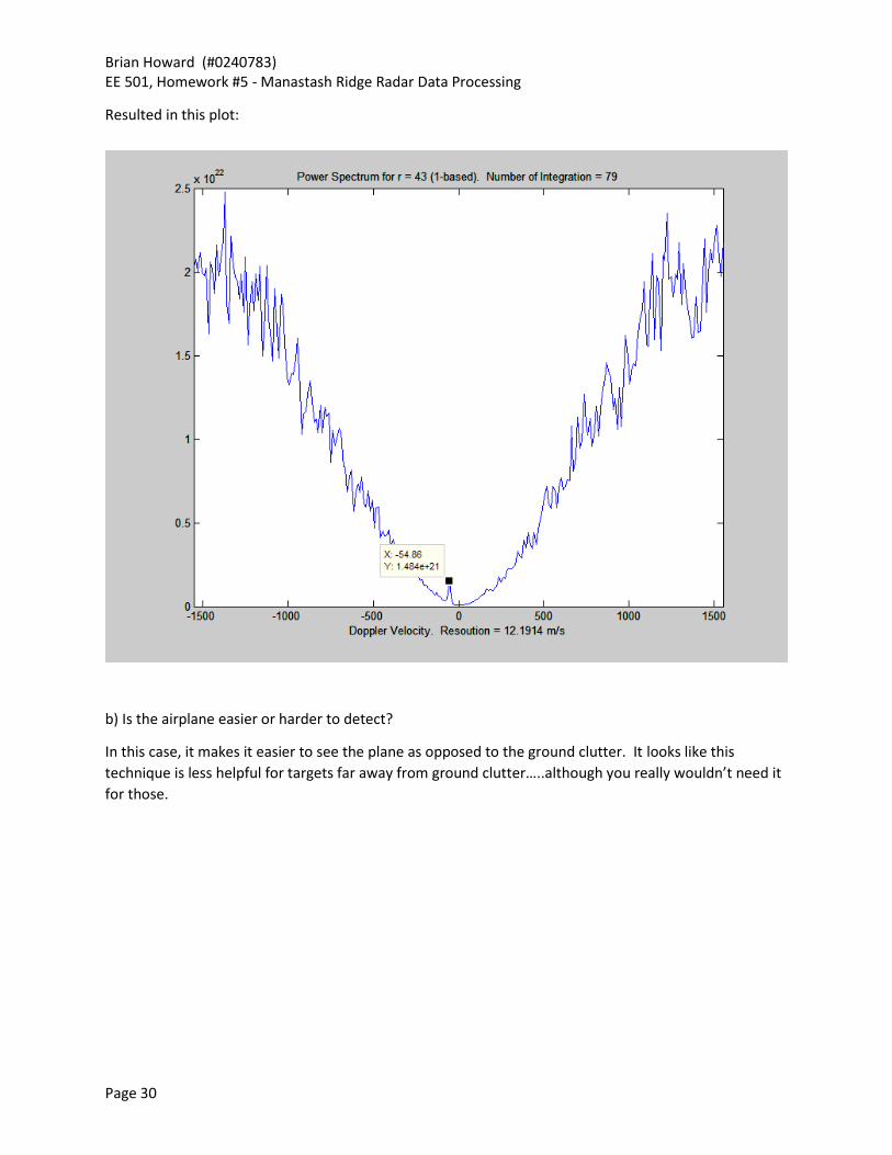
Problem 6. MTI (”moving target indicator”) processing. Ground clutter always appears with very low
Doppler Velocity, so it would be nice to reject it, if possible. Rather than using Z(m,r) directly, create a
new data set,
Z1(m,r) = Z(m,r) − Z(m − 1,r) (3)
a) Plot the power spectrum of Z1(m,r = 42)?
This is the code
% EE501 Homework 5, Problem 6(a)
% Brian Howard, 9 June 2013
clear all;
close all;
home;
mat_size = 4096000/2;
N = mat_size/2;
c = 300000000;
fb = 96500000;
lambda = c/fb;
D = 50;
fs = 100000;
% Only need to run these lines once. Just load it otherwise
if 0
strFileName = 'ref.dat';
fid = fopen(strFileName, 'r');
tmp=fread(fid, mat_size,'short');
ref=complex(tmp(1:2:mat_size),tmp(2:2:mat_size));
strFileName = 'sca.dat';
fid = fopen(strFileName, 'r');
tmp=fread(fid, mat_size,'short');
sca=complex(tmp(1:2:mat_size),tmp(2:2:mat_size));
r = 1:801;
m = 1:(fix((N-max(r))/D));
Z = zcorr(sca, ref, m, r, D);
save('Z800.mat','Z');
end
load('Z800');
% Create the Z1 Array: Z1(m,r) = Z(m,r) ? Z(m ? 1,r)
iOffset = 1;
Z = Z-circshift(Z,[-iOffset,0]);
Z(:,1:iOffset)=[];
% calculate the power estimate
M = min(size(Z));
Pest = zeros(M,1);
for r = 1:M
P(r) = dot(Z(:,r),Z(:,r));
P(r) = P(r)./M;
end
% calculate the range in km
rd = (0:(M-1)).*(1/fs)*(c/2)*0.001;
% coherent integration
r = 43;
n = 256;
[len rng] = size(Z);
Y = zeros(n,rng);
for iRng = 1:rng
Brian Howard (#0240783) EE 501, Homework #5 - Manastash Ridge Radar Data Processing
Page 29
for iCorr = 0:(fix(len/n)-1)
Y(:,iRng) = Y(:,iRng) + fftshift(abs(fft(Z((iCorr*n)+1:(iCorr+1)*n,iRng))).^2);
end
end
fd = (fs/(2*D))*lambda/2;
fds =((-(n-1)/2):((n-1)/2))./((n-1)/2);
fds = fds.*fd;
figure('Name','Problem 6 - a','position',[1 1 800 600])
plot(fds,Y(:,r));
title(['Power Spectrum for r = ' num2str(r) ' (1-based). Number of Integration = '
num2str(fix(len/n))])
xlabel(['Doppler Velocity. Resoution = ' num2str(fds(2)-fds(1)) ' m/s']);
xlim([min(fds) max(fds)]);
Brian Howard (#0240783) EE 501, Homework #5 - Manastash Ridge Radar Data Processing
Page 30
Resulted in this plot:
b) Is the airplane easier or harder to detect?
In this case, it makes it easier to see the plane as opposed to the ground clutter. It looks like this
technique is less helpful for targets far away from ground clutter…..although you really wouldn’t need it
for those.
Brian Howard (#0240783) EE 501, Homework #5 - Manastash Ridge Radar Data Processing
Page 31
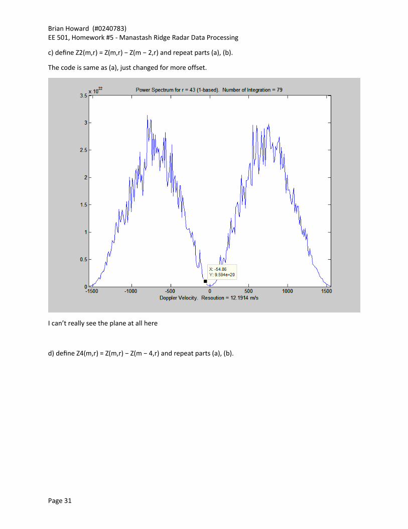
c) define Z2(m,r) = Z(m,r) − Z(m − 2,r) and repeat parts (a), (b).
The code is same as (a), just changed for more offset.
I can’t really see the plane at all here
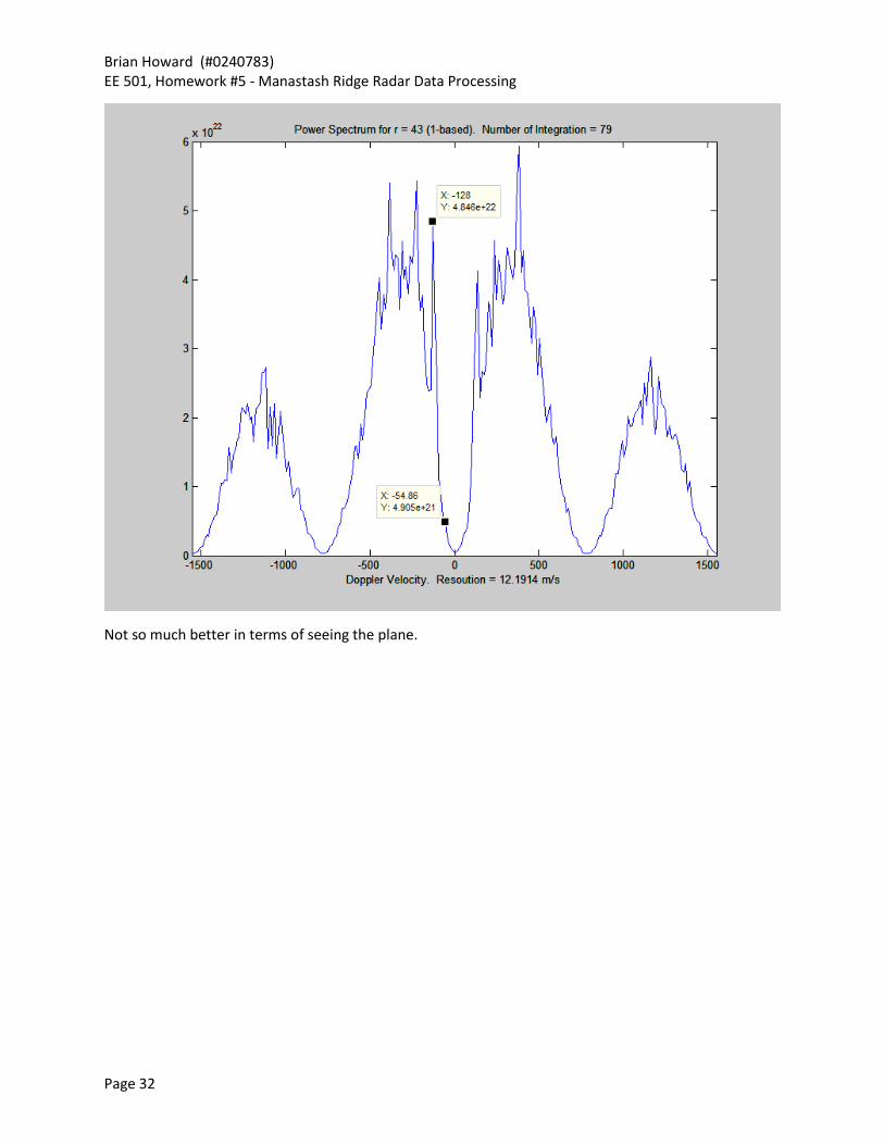
d) define Z4(m,r) = Z(m,r) − Z(m − 4,r) and repeat parts (a), (b).
Brian Howard (#0240783) EE 501, Homework #5 - Manastash Ridge Radar Data Processing
Page 32
Not so much better in terms of seeing the plane.
Brian Howard (#0240783) EE 501, Homework #5 - Manastash Ridge Radar Data Processing
Page 33
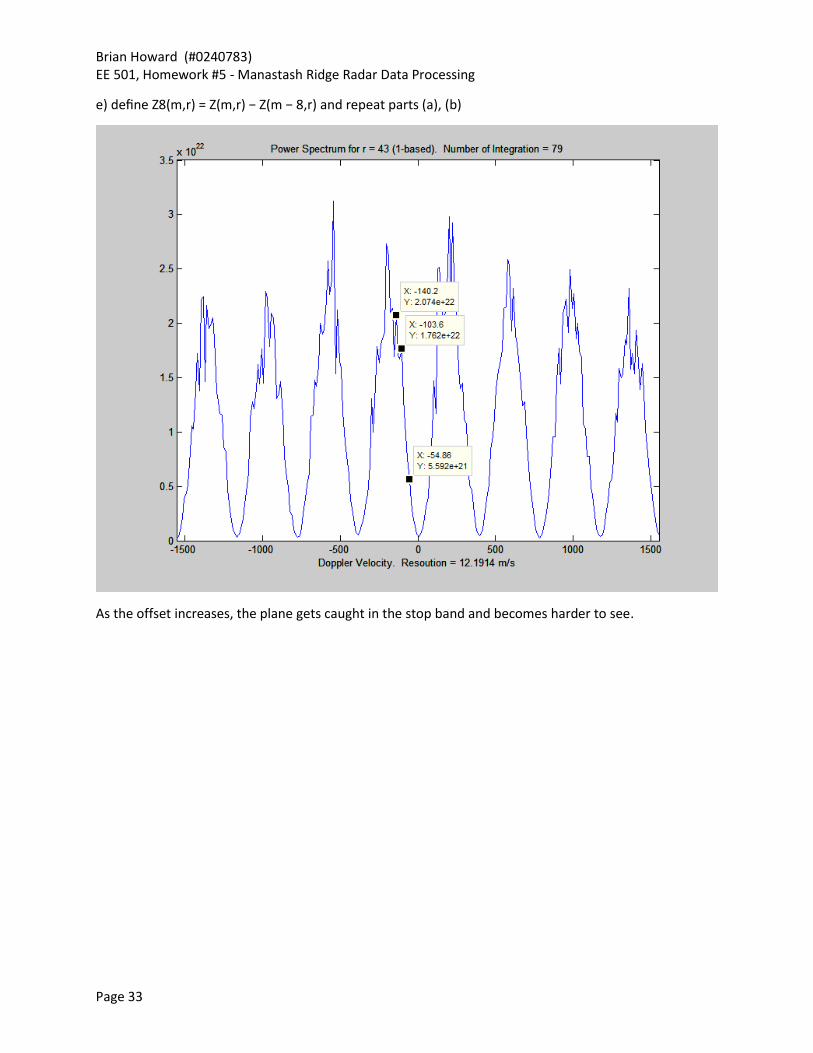
e) define Z8(m,r) = Z(m,r) − Z(m − 8,r) and repeat parts (a), (b)
As the offset increases, the plane gets caught in the stop band and becomes harder to see.

Brian Howard (#0240783) EE 501, Homework #5 - Manastash Ridge Radar Data Processing
Page 34
Problem 7. Assume that the airplane at range 44-45 is flying at an altitude of 5000m. Describe the locus
of its possible locations. You’ll need the following data; KJAQ is the 96.5 MHz transmitter. The first two
numbers in the URL are the latitude and longitude. MRO is where the sca.dat data is taken; Sieg is where
ref.dat is taken, and KJAQ is the location of the transmitter. Note that negative longitude is ”west”.
UWSieg http://maps.google.com/?ll=47.654955,-122.306636&spn=0.000383,0.000536&t=h&z=21
MRO http://maps.google.com/?ll=46.951011,-120.724901&spn=0.000548,0.001072&t=h&z=20
KJAQ http://maps.google.com/?ll=47.504546,-121.969182&spn=0.000543,0.001072&t=h&z=20
Use the ref and transmitter location to offset the time delay incurred between them. With the
corrected signal you can draw an ellipse of constant range, with foci at the transmitter and at the
antenna for sca.
Brian Howard (#0240783) EE 501, Homework #5 - Manastash Ridge Radar Data Processing
Page 35
Problem 8. There is an additional data set you can use for the scatter data:
http://rrsl.ee.washington.edu/ee501/scb.dat
This data was taken at exactly the same time as sca.dat, but on a different antenna.
a) When you process scb.dat, do you see the same spectral signatures as with sca.dat?
Using this code:
% EE501 Homework 5, Problem 8(a)
% Brian Howard, 7 June 2013
clear all;
close all;
home;
mat_size = 4096000/2;
N = mat_size/2;
c = 300000000;
fb = 96500000;
lambda = c/fb;
D = 50;
fs = 100000;
% Only need to run these lines once. Just load it otherwise
if 0
strFileName = 'ref.dat';
fid = fopen(strFileName, 'r');
tmp=fread(fid, mat_size,'short');
ref=complex(tmp(1:2:mat_size),tmp(2:2:mat_size));
strFileName = 'scb.dat';
fid = fopen(strFileName, 'r');
tmp=fread(fid, mat_size,'short');
sca=complex(tmp(1:2:mat_size),tmp(2:2:mat_size));
r = 1:801;
m = 1:(fix((N-max(r))/D));
Z = zcorr(sca, ref, m, r, D);
save('Z800b.mat','Z');
end
load('Z800b');
% calculate the power estimate
M = min(size(Z));
Pest = zeros(M,1);
for r = 1:M
P(r) = dot(Z(:,r),Z(:,r));
P(r) = P(r)./M;
end
% calculate the range in km
rd = (0:(M-1)).*(1/fs)*(c/2)*0.001;
% coherent integration
r = 43;
n = 256;
[len rng] = size(Z);
Y = zeros(n,rng);
for iRng = 1:rng
for iCorr = 0:(fix(len/n)-1)
Y(:,iRng) = Y(:,iRng) + fftshift(abs(fft(Z((iCorr*n)+1:(iCorr+1)*n,iRng))).^2);
end
end
fd = (fs/(2*D))*lambda/2;
fds =((-(n-1)/2):((n-1)/2))./((n-1)/2);
Brian Howard (#0240783) EE 501, Homework #5 - Manastash Ridge Radar Data Processing
Page 36
fds = fds.*fd;
figure('Name','Problem 8 - a','position',[1 1 800 600])
plot(fds,Y(:,r));
title(['Power Spectrum for r = ' num2str(r) ' (1-based). Number of Integration = '
num2str(fix(len/n))])
xlabel(['Doppler Velocity. Resoution = ' num2str(fds(2)-fds(1)) ' m/s']);
xlim([min(fds) max(fds)]);
% plot the data
figure('Name','Problem 8 - a','position',[1 1 800 600])
imagesc([min(fds) max(fds)], [1 max(rd)], (log10(Y)'))
title(['Log of Power Spectrum. Number of Integration = ' num2str(fix(len/n))])
xlabel(['Doppler Velocity. Resoution = ' num2str(fds(2)-fds(1)) ' m/s']);
ylabel('Distance, km');
set(gca,'YDir','normal')
%caxis([21.5 24])
colorbar
figure('Name','Problem 8 - a','position',[1 1 800 600])
hSurf = surf((log10(Y)'),'EdgeColor','none','LineStyle','none','FaceColor','interp');
camproj('orthographic')
set(gca,'YDir','normal')
%caxis([21.5 24])
view([-31.5 24]);
colorbar

Brian Howard (#0240783) EE 501, Homework #5 - Manastash Ridge Radar Data Processing
Page 37
The code gives this figure below:
I see some of the same ground clutter features visible with the other antenna; however the planes and
the turbulence do not look to be visible.

Brian Howard (#0240783) EE 501, Homework #5 - Manastash Ridge Radar Data Processing
Page 38
b) In addition to computing the cross ambiguity for each antenna, you can also compute the cross
coherence of each antenna:
𝐶(𝑟, 𝑓) =
𝐸(𝑉𝑎(𝑟, 𝑓)𝑉𝑏∗(𝑟, 𝑓))
√𝐸(𝑉𝑎(𝑟, 𝑓)𝑉𝑎∗(𝑟, 𝑓))√𝐸(𝑉𝑏(𝑟, 𝑓)𝑉𝑏
∗(𝑟, 𝑓))
(4)
Here Va(r,f) is an individual voltage spectrum for antenna a. The magnitude and phase of C tells you
about the angular size and direction at range r and Doppler shift f.
Using this code:
% EE501 Homework 5, Problem 8(a)
% Brian Howard, 7 June 2013
clear all;
close all;
home;
mat_size = 4096000/2;
N = mat_size/2;
c = 300000000;
fb = 96500000;
lambda = c/fb;
D = 50;
fs = 100000;
% Only need to run these lines once. Just load it otherwise
if 0
strFileName = 'ref.dat';
fid = fopen(strFileName, 'r');
tmp=fread(fid, mat_size,'short');
ref=complex(tmp(1:2:mat_size),tmp(2:2:mat_size));
strFileName = 'scb.dat';
fid = fopen(strFileName, 'r');
tmp=fread(fid, mat_size,'short');
sca=complex(tmp(1:2:mat_size),tmp(2:2:mat_size));
r = 1:801;
m = 1:(fix((N-max(r))/D));
Z = zcorr(sca, ref, m, r, D);
save('Z800b.mat','Z');
end
load('Z800b');
Zb=Z;
load('Z800');
% calculate the power estimate
M = min(size(Z));
Pest = zeros(M,1);
for r = 1:M
P(r) = dot(Z(:,r),Z(:,r));
P(r) = P(r)./M;
end
% calculate the range in km
rd = (0:(M-1)).*(1/fs)*(c/2)*0.001;
% coherent integration
Brian Howard (#0240783) EE 501, Homework #5 - Manastash Ridge Radar Data Processing
Page 39
r = 43;
n = 256;
[len rng] = size(Z);
Y = zeros(n,rng);
Yb = zeros(n,rng);
C = zeros(n,rng);
Va = zeros(n, fix(len/n));
Vb = zeros(n, fix(len/n));
for iRng = 1:rng
for iCorr = 0:(fix(len/n)-1)
Va(:,iCorr+1) = fftshift((fft(Z((iCorr*n)+1:(iCorr+1)*n,iRng))).^2);
Y(:,iRng) = Y(:,iRng) + abs(Va(:,iCorr+1));
Vb(:,iCorr+1) = fftshift((fft(Zb((iCorr*n)+1:(iCorr+1)*n,iRng))).^2);
Yb(:,iRng) = Yb(:,iRng) + abs(Vb(:,iCorr+1));
end
% Cross-coherence for this range
for fc = 1:n
C(fc,iRng) = mean(Va(fc,1:end).*conj(Vb(fc,1:end)));
C(fc,iRng) = C(fc,iRng)./sqrt(mean(Va(fc,1:end).*conj(Va(fc,1:end))));
C(fc,iRng) = C(fc,iRng)./sqrt(mean(Vb(fc,1:end).*conj(Vb(fc,1:end))));
end
end
fd = (fs/(2*D))*lambda/2;
fds =((-(n-1)/2):((n-1)/2))./((n-1)/2);
fds = fds.*fd;
figure('Name','Problem 8 - b','position',[1 1 800 600])
plot(fds,Y(:,r));
title(['Power Spectrum for r = ' num2str(r) ' (1-based). Number of Integration = '
num2str(fix(len/n))])
xlabel(['Doppler Velocity. Resoution = ' num2str(fds(2)-fds(1)) ' m/s']);
xlim([min(fds) max(fds)]);
% plot the data
figure('Name','Problem 8 - b','position',[1 1 800 600])
imagesc([min(fds) max(fds)], [1 max(rd)], (log10(Y)'))
title(['Log of Power Spectrum, B Antenna. Number of Integration = ' num2str(fix(len/n))])
xlabel(['Doppler Velocity. Resoution = ' num2str(fds(2)-fds(1)) ' m/s']);
ylabel('Distance, km');
set(gca,'YDir','normal')
%caxis([21.5 24])
colorbar
% plot the data
figure('Name','Problem 8 - b','position',[1 1 800 600])
imagesc([min(fds) max(fds)], [1 max(rd)], (log10(Yb)'))
title(['Log of Power Spectrum, B Antenna. Number of Integration = ' num2str(fix(len/n))])
xlabel(['Doppler Velocity. Resoution = ' num2str(fds(2)-fds(1)) ' m/s']);
ylabel('Distance, km');
set(gca,'YDir','normal')
%caxis([21.5 24])
colorbar
% plot the data
figure('Name','Problem 8 - b','position',[1 1 800 600])
imagesc([min(fds) max(fds)], [1 max(rd)], (abs(C)'))
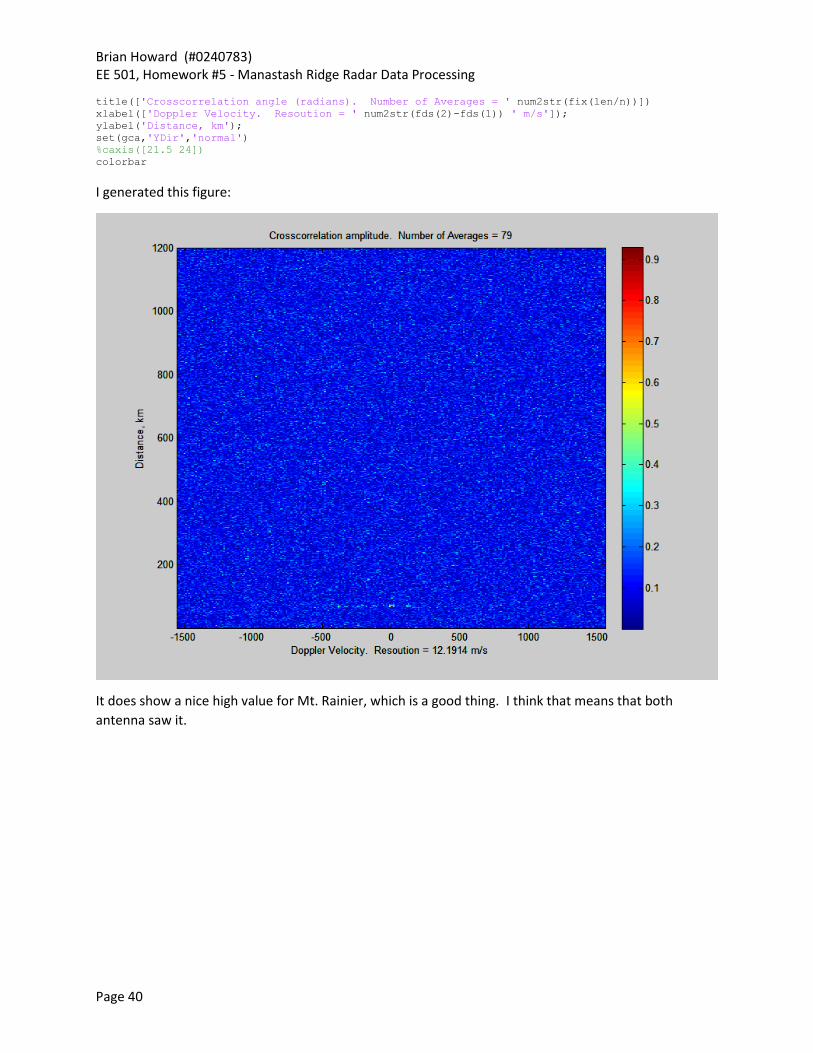
title(['Crosscorrelation amplitude. Number of Averages = ' num2str(fix(len/n))])
xlabel(['Doppler Velocity. Resoution = ' num2str(fds(2)-fds(1)) ' m/s']);
ylabel('Distance, km');
set(gca,'YDir','normal')
%caxis([21.5 24])
colorbar
% plot the data
figure('Name','Problem 8 - b','position',[1 1 800 600])
imagesc([min(fds) max(fds)], [1 max(rd)], (angle(C)'))
Brian Howard (#0240783) EE 501, Homework #5 - Manastash Ridge Radar Data Processing
Page 40
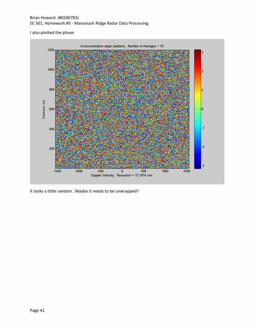
title(['Crosscorrelation angle (radians). Number of Averages = ' num2str(fix(len/n))])
xlabel(['Doppler Velocity. Resoution = ' num2str(fds(2)-fds(1)) ' m/s']);
ylabel('Distance, km');
set(gca,'YDir','normal')
%caxis([21.5 24])
colorbar
I generated this figure:
It does show a nice high value for Mt. Rainier, which is a good thing. I think that means that both
antenna saw it.
Brian Howard (#0240783) EE 501, Homework #5 - Manastash Ridge Radar Data Processing
Page 41
I also plotted the phase:
It looks a little random. Maybe it needs to be unwrapped?

Brian Howard (#0240783) EE 501, Homework #5 - Manastash Ridge Radar Data Processing
Page 42

Brian Howard (#0240783) EE 501, Homework #5 - Manastash Ridge Radar Data Processing
Page 43


![A novel approach for vector quantization using a neural …techlab.bu.edu/files/resources/articles_tt/[SignalProcessing]v87_i... · A novel approach for vector quantization using](https://img.pdfslide.net/doc/110x75/5b25660b7f8b9aa64b8b729e/a-novel-approach-for-vector-quantization-using-a-neural-signalprocessingv87i.jpg)