Embed Size (px)
Citation preview
Purdue UniversityPurdue e-Pubs
Open Access Dissertations Theses and Dissertations
12-2016
Bridge maintenance to enhance corrosionresistance and performance of steel girder bridgesLuis M. Moran YanezPurdue University
Follow this and additional works at: https://docs.lib.purdue.edu/open_access_dissertations
Part of the Civil Engineering Commons, and the Materials Science and Engineering Commons
This document has been made available through Purdue e-Pubs, a service of the Purdue University Libraries. Please contact [email protected] foradditional information.
Recommended CitationMoran Yanez, Luis M., "Bridge maintenance to enhance corrosion resistance and performance of steel girder bridges" (2016). OpenAccess Dissertations. 977.https://docs.lib.purdue.edu/open_access_dissertations/977

Graduate School Form
30 Updated
PURDUE UNIVERSITY
GRADUATE SCHOOL
Thesis/Dissertation Acceptance
This is to certify that the thesis/dissertation prepared
By
Entitled
For the degree of
Is approved by the final examining committee:
To the best of my knowledge and as understood by the student in the Thesis/Dissertation
Agreement, Publication Delay, and Certification Disclaimer (Graduate School Form 32),
this thesis/dissertation adheres to the provisions of Purdue University’s “Policy of
Integrity in Research” and the use of copyright material.
Approved by Major Professor(s):
Approved by:
Head of the Departmental Graduate Program Date

i
BRIDGE MAINTENANCE TO ENHANCE CORROSION RESISTANCE AND
PERFORMANCE OF STEEL GIRDER BRIDGES
A Dissertation
Submitted to the Faculty
of
Purdue University
by
Luis M. Moran Yañez
In Partial Fulfillment of the
Requirements for the Degree
of
Doctor of Philosophy
December 2016
Purdue University
West Lafayette, Indiana
iv
the Indiana Department of Transportation and its staff, by supporting my research with
information, materials and guidance.
My deeply thanks to my mother, brothers and sister, because I always have in mind all
what they did for me. To Clarita, Luis Miguel and Paquito, for being with me in this
project, for their love and affection. To Clara, my wife, by joining me in my dreams and
goals, for her love and constant encouragement.
v
TABLE OF CONTENTS
Page
LIST OF TABLES ............................................................................................................. xi
LIST OF FIGURES ......................................................................................................... xiv
ABSTRACT ..................................................................................................................... xxi
INTRODUCTION ................................................................................. 1
1.1 General ..................................................................................................................... 1
1.2 Problem Statement ................................................................................................... 1
1.3 Objectives of the Research ....................................................................................... 6
1.4 Scope of the Research .............................................................................................. 7
LITERATURE REVIEW ...................................................................... 9
2.1 Research on Atmospheric Corrosion of Steel Girder Highway Bridges .................. 9
2.2 Research in Bridge Maintenance Activities ........................................................... 12
2.3 Research on Accelerated Corrosion Tests .............................................................. 15
2.4 Research on Structural Analysis and Design of Corroded Composite Steel
Girders .......................................................................................................................... 16
CORROSION OF STEEL BRIDGE HIGHWAY GIRDERS ............ 18
3.1 Introduction ............................................................................................................ 18
3.2 Structural Steel ....................................................................................................... 18
3.2.1 Characteristics of Structural Steel .....................................................................18
3.2.2 Types of Structural Steel for Bridges ................................................................20
3.3 Corrosion of Structural Steel .................................................................................. 22
3.3.1 Definition of Corrosion .....................................................................................22
3.3.2 Atmospheric Corrosion .....................................................................................23
3.3.3 Electrochemical Corrosion Process ...................................................................24
vi
Page
3.3.4 Forms of Corrosion ............................................................................................26
3.3.5 Atmospheric Environments ...............................................................................27
3.4 Corrosion of Composite Steel Girders ................................................................... 28
3.4.1 Causes of Steel Girder Corrosion ......................................................................28
3.4.2 Problems Due to Steel Girder Corrosion ...........................................................30
3.5 Deterioration Model of Steel Girder Corrosion ..................................................... 32
3.5.1 Model to Predict the Rate of Corrosion .............................................................32
3.5.2 Model to Predict Location of Corrosion ............................................................37
3.6 Corrosion Protection of Steel Girders .................................................................... 40
MAINTENANCE ACTIVITIES OF STEEL GIRDER BRIDGES .... 42
4.1 Introduction ............................................................................................................ 42
4.2 Bridge Superstructure Washing .............................................................................. 43
4.2.1 Bridge Superstructure Washing Programs at State DOTs .................................45
4.2.2 Bridge Superstructure Washing Benefits ..........................................................49
4.3 Spot Painting .......................................................................................................... 50
4.3.1 Spot Painting Benefits .......................................................................................51
4.3.2 Service Life of Spot Painting.............................................................................52
4.4 Summary ................................................................................................................ 53
ACCELERATED CORROSION TEST .............................................. 54
5.1 Introduction ............................................................................................................ 54
5.2 Accelerated Corrosion Test Program ..................................................................... 56
5.2.1 Accelerated Corrosion Test – ASTM B117 ......................................................56
5.2.2 Materials ............................................................................................................57
5.2.3 Equipment ..........................................................................................................59
5.2.4 Salt Solution Application...................................................................................63
5.3 ACT for Steel Washing Evaluation ........................................................................ 64
5.3.1 Number of Coupons and Identification .............................................................64
5.3.2 Schedule for Washing Process ..........................................................................65
5.3.3 Initial Data Acquisition .....................................................................................67
vii
Page
5.3.4 Procedure for the ACT Regime for Steel Washing Evaluation .........................69
5.3.5 Results from ACT for Steel Washing Evaluation .............................................74
5.4 ACT for Spot Painting Evaluation ......................................................................... 91
5.4.1 Number of Coupons and Identification .............................................................91
5.4.2 Scribing Coupon Procedure ...............................................................................92
5.4.3 Initial Data Acquisition .....................................................................................93
5.4.4 Procedure for the ACT Regime for Spot Painting Evaluation ..........................93
5.4.5 Results from ACT for Spot Painting Evaluation ...............................................96
5.5 Discussion of Results ........................................................................................... 105
5.5.1 Accelerated Corrosion Test (ACT) .................................................................105
5.5.2 Steel Washing Evaluation ................................................................................106
5.5.3 Spot Painting Evaluation .................................................................................107
CORRELATION BETWEEN AN ACCELERATED CORROSION
TEST AND ATMOSPHERIC CORROSION ................................................................ 108
6.1 Introduction .......................................................................................................... 108
6.2 Control Test .......................................................................................................... 110
6.2.1 Number of Coupons and Identification ...........................................................110
6.2.2 Schedule for Control Test ................................................................................110
6.2.3 Initial Data Acquisition ...................................................................................111
6.2.4 Procedure for the Control Test ........................................................................111
6.2.5 Results from Control Test ...............................................................................112
6.3 Correlation between ACT and Atmospheric Corrosion ....................................... 118
6.3.1 Correlation between the Weight Increment and Corrosion Penetration during
ACT ......................................................................................................................... 118
6.3.2 Correlation between Time inside the Chamber and Time at Real
Environments ........................................................................................................... 120
6.3.3 Correlation between Corrosion Penetration from ACT to Atmospheric
Corrosion ................................................................................................................. 124
6.4 Sensitivity Analysis between Control Test Data and ACT Data .......................... 131
viii
Page
STRUCTURAL ANALYSIS, DESIGN, AND LOAD RATING ..... 139
7.1 Introduction .......................................................................................................... 139
7.2 Bridge Load and Resistant Models ...................................................................... 140
7.2.1 Dead Load .......................................................................................................140
7.2.2 Live Load .........................................................................................................141
7.2.3 Dynamic Load .................................................................................................142
7.2.4 Bridge Resistance Model .................................................................................143
7.3 Structural Analysis and Design According to AASHTO LRFD .......................... 143
7.3.1 Representative I-Girder Steel Bridges Considered ..........................................144
7.3.2 Design Parameters and Loading Considerations .............................................148
7.3.3 Load and Resistance Factor Design (AASHTO LRFD) .................................149
7.3.4 Limit States ......................................................................................................150
7.3.5 Design for Flexural Capacity ...........................................................................151
7.3.6 Design for Shear Capacity ...............................................................................153
7.3.7 Elastic Deflections ...........................................................................................154
7.3.8 Steel Highway Bridge Design using a FE Package .........................................154
7.3.9 Analysis and Design of Typical Steel Girder Bridge ......................................157
7.4 Steel Bridge Load Rating According to AASHTO MBE .................................... 163
7.4.1 Load and Resistance Factor Rating (LRFR)....................................................163
7.4.2 General Load-Rating Equation ........................................................................166
7.4.3 Levels of Evaluation ........................................................................................168
7.4.4 Load Rating for Representative Bridges Considered ......................................172
7.5 Results and Discussion ......................................................................................... 175
7.5.1 Effect of Stress Type .......................................................................................177
7.5.2 Effect of Local Environment ...........................................................................181
7.5.3 Effect of Number of Spans ..............................................................................183
7.5.4 Effect of Span Length ......................................................................................185
7.5.5 Effect of Steel Type .........................................................................................187
7.5.6 Effect on Live-Load Deflections .....................................................................189
ix
Page
7.5.7 Effect of Maintenance Alternative ..................................................................193
ECONOMIC EVALUATION OF CORRODED STEEL BRIDGES198
8.1 Introduction .......................................................................................................... 198
8.2 Life Cycle Cost Analysis ...................................................................................... 199
8.2.1 Bridge Service Life ..........................................................................................200
8.2.2 Cost of Bridge Maintenance Activities, Rehabilitation, and Replacement .....200
8.2.3 Discount Rate ..................................................................................................201
8.2.4 Present Value ...................................................................................................201
8.2.5 Bridge Load Rating .........................................................................................202
8.3 Economic Analysis for Bridge Maintenance Activities ....................................... 205
8.3.1 Effect of Steel Girder Washing Activity for Uncoated Carbon Steel .............205
8.3.2 Effect of Steel Girder Washing Activity for Coated Carbon Steel .................209
8.3.3 Effect of Washing on Coated and Re-coated Carbon Steel Members .............213
8.3.4 Effect of Steel Washing Activity for Uncoated and Coated Weathering
Steel ......................................................................................................................... 215
8.4 Results from LCCA .............................................................................................. 217
SUMMARY, CONCLUSIONS AND RECOMMENDATIONS ..... 219
9.1 Summary .............................................................................................................. 219
9.2 Conclusions .......................................................................................................... 221
9.3 Recommendations ................................................................................................ 224
LIST OF REFERENCES ................................................................................................ 226
APPENDICES
Appendix A Corrosion Penetration Data ................................................................... 235
Appendix B Product Certificate................................................................................. 239
Appendix C Identification of Coupons for ACT ....................................................... 243
Appendix D Weight Change During ACT................................................................. 246
Appendix E Initial Dimensions of Coupons .............................................................. 264
Appendix F Thickness Change During ACT ............................................................ 268
Appendix G Photographs During ACT...................................................................... 284

x
Page
Appendix H Creepage Area Change of Scribed Coupons During ACT .................... 288
Appendix I Control Test ........................................................................................... 294
Appendix J Rating Factors RFm and RFv ................................................................ 298
VITA ............................................................................................................................... 323
xi
LIST OF TABLES
Table .............................................................................................................................. Page
3.1: Minimum mechanical properties of structural steel by shape, strength, and thickness
(AASHTO, 2012) ......................................................................................................... 21
3.2: Statistical parameters for A and B (Kayser, 1988) .................................................... 34
4.1: DOTs information reported on bridge washing programs (Berman et al., 2013) .... 46
4.2: Service life of spot painting (Bowman and Moran, 2015) ........................................ 53
5.1: Matrix for washing program ...................................................................................... 66
6.1: Results of Control Test for coupons from steel Type A. ......................................... 114
6.2: Results of Control Test for coupons from steel Type C .......................................... 116
6.3: Corrosion penetration values from ACT for steel Type A ...................................... 119
6.4: Corrosion penetration values from ACT for steel Type C....................................... 120
6.5: Correlating weeks in Control Test - years at real environments – (Type A) ........... 121
6.6: Correlating weeks in Control Test - years at real environments – (Type C) ........... 122
6.7: Correlating values between ACT and real environments – steel Type A ................ 123
6.8: Correlating values between ACT and real environments - steel Type C................. 124
6.9: Corrosion penetration C for steel Type A versus time measured in weeks at ACT
and years at real environments ................................................................................... 126
6.10: Corrosion penetration C for steel Type C versus time measured in weeks at ACT
and years at real environments ................................................................................... 127
6.11: Weight increment data from control test and Group A10 ..................................... 131
6.12: Ratio of corrosion penetration to weight increment for control test data .............. 132
6.13: Corrosion penetration from weight increment for Group A10 .............................. 132
6.14: Corrosion penetration values from Group A10 ..................................................... 134
6.15: Correlating penetration from Group A10 with years at real environments ........... 135
xii
Table .............................................................................................................................. Page
6.16: Correlating years at real environments for 3.5 weeks at ACT – Steel Type A ..... 136
6.17: Corrosion penetration C for steel type A versus time measured in weeks at ACT
and years at real environments ................................................................................... 136
7.1: Typical values for materials weight ......................................................................... 140
7.2: Dynamic load allowance (AASHTO, 2012) ............................................................ 143
7.3: Material properties assumed for composite steel girder bridges ............................. 148
7.4: Multiple presence factors, m (AASHTO, 2012) ...................................................... 149
7.5: Dead load moment values for CSiBridge and hand solution and analysis .............. 156
7.6: Live load moment values for hand solution and CSiBridge analysis ...................... 157
7.7: Maximum Demand/Capacity ratios for stresses and deflections ............................. 162
7.8: Generalized live load factors for commercial routine vehicles - Evaluation for
strength I limit state (AASHTO, 2011) ...................................................................... 172
7.9: Generalized live load factors for specialized hauling vehicles - Evaluation for
strength I limit state (AASHTO, 2011) ...................................................................... 172
8.1: Unit costs for bridge maintenance activities (Sobanjo, 2001; Hearn, 2012) ........... 201
8.2: Bridge’s service age (years) when reaching RFv=1.0 - Industrial/urban ................ 204
8.3: Bridge’s service age (years) when reaching RFv=1.0 - Marine .............................. 204
8.4: Bridge’s service age (years) when reaching RFv=1.0 - Rural ................................. 205
8.5: Bridge models reaching legal load rating limit RFv = 1.00 .................................... 209
8.6: Three-coat paint system service life ........................................................................ 210
8.7: Summary of PV for bridge cases of carbon steel, uncoated and coated .................. 213
Appendix Table
A.1: Parameters A and B – Industrial environment. Albrecht and Naeemi (1984) ........ 235
A.2: Parameters A and B –Marine environment. Albrecht and Naeemi (1984) ............. 235
A.3: Parameters A and B – Rural environment. Albrecht and Naeemi (1984) .............. 236
C.1: Identification of steel coupons from steel types A, B, C, and D ............................. 244
D.1: Weight change during ACT for coupons from steel Type A .................................. 247
D.2: Weight change during ACT for coupons from steel Type B .................................. 252
D.3: Weight change during ACT for coupons from steel Type C .................................. 257
xiii
Appendix Table .............................................................................................................. Page
D.4: Weight change during ACT for coupons from steel Type D .................................. 262
E.1: Initial dimensions of coupons from steel Type A ................................................... 265
E.2: Initial dimensions of coupons from steel Type B.................................................... 266
E.3: Initial dimensions of coupons from steel Type C.................................................... 267
F.1: Thickness change during ACT for coupons from steel Type A .............................. 269
F.2: Thickness change during ACT for coupons from steel Type B .............................. 274
F.3: Thickness change during ACT for coupons from steel Type C .............................. 279
H.1: Creepage area change during ACT for coupons from steel Type D ....................... 291
I.1: Identification for Control Test coupons, Groups X and W ...................................... 295
I.2: Weight change for Control Test, Groups X.............................................................. 296
I.3: Weight change for Control Test, Groups W ............................................................. 296
xiv
LIST OF FIGURES
Figure ............................................................................................................................. Page
1.1: US bridge inventory by year of construction (FHWA, 2015) ..................................... 2
1.2: US steel bridges condition at 2005 (Eom, 1024) ......................................................... 3
1.3: Service life extension: a) Performing simple preventive maintenance activities, b)
Performing only important rehabilitation processes (NYSDOT, 2008) ......................... 5
3.1: Engineering stress-strain curve for structural steel (FHWA, 2012) .......................... 20
3.2: Classification of corrosion process (Syed, 2006) ...................................................... 23
3.3: Schematic representation of the corrosion mechanism for steel (Corus, 2005) ........ 25
3.4: Sketches for the principal forms of steel corrosion (Landolfo, 2010) ....................... 27
3.5: Typical corrosion process of steel girders: 1) at the web and bottom flange (Zaffetti,
2010), 2) Next to a pin and hanger connection (WisDOT, 2011) ................................ 30
3.6: Debris accumulation at a steel superstructure connection point (Kogler, 2012) ....... 30
3.7: Mean of Time-Corrosion penetration curves for carbon steel (Kayser, 1988) .......... 36
3.8: Corrosion penetration curves (Park et al., 1998) ....................................................... 37
3.9: Typical corrosion locations on a steel girder bridge (Kayser, 1988) ......................... 38
3.10: Corrosion on typical steel girder sections, at midspan (left), and at supports (right)
(Park, 1999) .................................................................................................................. 39
3.11: Corrosion on typical steel girder section (Czarnecki, 2006) ................................... 40
4.1: Damaged steel girder due to extended corrosion (Zaffetti, 2010) ............................. 44
4.2: Steel bridge superstructure washing (Crampton et al., 2013) .................................... 45
4.3: Interior of lower chord from truss. Before (left) and after (right) cleaning and
washing (Berman et al., 2013) ...................................................................................... 50
4.4: Portion of a steel girder candidate for spot painting (Myers et al., 2010) ................. 51
xv
Figure ............................................................................................................................. Page
5.1: Steel coupons before and after epoxy coating application. Left: uncoated coupon,
Right: coated coupon. ................................................................................................... 58
5.2: Steel coupons supported by PVC racks. .................................................................... 58
5.3: Front and lateral view of acrylic box ......................................................................... 59
5.4: Interior view of weather chamber with acrylic boxes (left). Misting system installed
(right) ............................................................................................................................ 61
5.5: Power washer ............................................................................................................. 62
5.6: Abrasive blast cabinet ................................................................................................ 62
5.7: Milling machine scribing a steel plate ....................................................................... 63
5.8: Components for salt solution preparation: Sodium chloride and scale (left), distilled
water and graduated plastic bucket (center), and pH-meter (right) .............................. 64
5.9: Location of thickness measuring positions ................................................................ 68
5.10: Coupon data acquisition. From left to right: weight, side dimensions, thickness,
photograph. ................................................................................................................... 69
5.11: Weather chamber with steel coupons under ACT regime. ...................................... 70
5.12: Power washing steel coupons .................................................................................. 71
5.13: Drying wet coupons after washing .......................................................................... 72
5.14: Flow chart for ACT program for steel washing evaluation ..................................... 74
5.15: Weight change versus time for steel Type A groups ............................................... 77
5.16: Weight change versus time for mean values from Groups A02-A05 and
Group A10 .................................................................................................................... 79
5.17: Weight change versus time for steel Type C groups ............................................... 80
5.18: Weight change versus time for mean values from Groups C02-C05 and
Group C10 .................................................................................................................... 81
5.19: Weight change versus time for steel Type C groups ............................................... 82
5.20: Weight change versus time for mean values from Groups B02-B05 and
Group B10 .................................................................................................................... 83
5.21: Thickness change versus time for steel Type A groups ........................................... 84
xvi
Figure ............................................................................................................................. Page
5.22: Thickness change versus time for mean values from Groups A02-A05 and
Group A10 .................................................................................................................... 85
5.23: Thickness change versus time for steel Type C groups ........................................... 87
5.24: Thickness change versus time for mean values from Groups C02-C05 and
Group C10 .................................................................................................................... 87
5.25: Thickness change versus time for steel Type B groups ........................................... 89
5.26: Thickness change versus time for mean values from Groups B02-B05 and
Group B10 .................................................................................................................... 89
5.27: Rust formation over uncoated steel coupon (coupon A01-a) .................................. 90
5.28: Lack of rust formation over coated steel coupon (coupon B05-a) .......................... 91
5.29: Left: Scribed steel coupon (D01-a). Right: Scribe mark magnified with (mm)
scale. ............................................................................................................................. 92
5.30: Flow chart for ACT program for spot painting evaluation ...................................... 94
5.31: Tools and products used to eliminate the rust and protect the scribe. ..................... 95
5.32: Process to clean and protect the scribe. From left to right: Clean the scribe with
sandpaper and rust dissolver application; cover all coupon face but scribe mark;
spray paint; coupon with covered scribe. ..................................................................... 96
5.33: Weight change versus time for steel Type D groups ............................................... 98
5.34: Weight change versus time for mean values from Groups D01-D04 and
Group D06 .................................................................................................................... 99
5.35: Creepage area measurement (ASTM Standard D7087-05a) ................................. 100
5.36: Trace of rust creepage area. Complete scribed coupon image and two
magnifications after six weeks of ACT. ..................................................................... 102
5.37: Net Mean Creepage versus time for steel Type D groups ..................................... 103
5.38: Net Mean Creepage versus time for mean values from Groups D02-D04 and
Group D06 .................................................................................................................. 104
5.39: Coupons from Groups D05 and D07 after the ACT ended ................................... 105
6.1: Dimensions for exposed area of a Control Test coupon .......................................... 113
6.2: Correlation weight increment-corrosion penetration for steel Type A .................... 115
xvii
Figure ............................................................................................................................. Page
6.3: Correlating weight increment-corrosion penetration for steel Type C .................... 117
6.4: Correlating weeks in Control Test - years at real environments - steel Type A ...... 123
6.5: Correlating weeks in Control Test - years at real environments - steel Type C ...... 124
6.6: Corrosion penetration vs. time - steel Type A - Industrial/Urban environment ...... 128
6.7: Corrosion penetration vs. time - steel Type A - Marine environment ..................... 128
6.8: Corrosion penetration vs. time - steel Type A - Rural environment........................ 129
6.9: Corrosion penetration vs. time - steel Type C - Industrial/Urban environment ...... 129
6.10: Corrosion penetration vs. time - steel Type C - Marine environment ................... 130
6.11: Corrosion penetration vs. time - steel Type C - Rural environment ...................... 130
6.12: Correlation weight increment-corrosion penetration for steel Type A .................. 133
6.13: Correlating weeks in the ACT with years at real environments – Type A ............ 135
6.14: Corrosion penetration vs. time – steel Type A – Industrial/urban environment .... 137
6.15: Corrosion penetration vs. time – steel Type C – Industrial/urban environment .... 138
7.1: AASHTO LRFD design live load (HL-93) (AASHTO, 2011) ............................... 142
7.2: Typical bridge cross section (Barth, 2012) .............................................................. 145
7.3: Sketch of longitudinal view for typical one-span and two-span bridges ................. 147
7.4: Sketch of typical steel girder elevation (Barth, 2012) ............................................. 156
7.5: Sketch of the typical 70’ one-span composite steel I-girder bridge ........................ 158
7.6: Sketch of the typical 90’ one-span composite steel I-girder bridge ........................ 158
7.7: Sketch of the typical 110’ one-span composite steel I-girder bridge ...................... 158
7.8: Sketch of the typical 130’ one-span composite steel I-girder bridge ...................... 159
7.9: Sketch of the typical 70’-70’ two-span composite steel I-girder bridge.................. 160
7.10: Sketch of the typical 90’-90’ two-span composite steel I-girder bridge ................ 160
7.11: Sketch of the typical 110’-110’ two-span composite steel I-girder bridge ............ 161
7.12: Sketch of the typical 130’-130’ two-span composite steel I-girder bridge ............ 161
7.13: Load and resistance factor rating flow chart (AASHTO, 2011) ............................ 165
7.14: AASHTO legal trucks (AASHTO, 2011) .............................................................. 170
7.15: Bridge posting loads for single-unit SHVs (AASHTO, 2011) .............................. 171
7.16: Notional rating load (AASHTO, 2011) ................................................................. 171
xviii
Figure ............................................................................................................................. Page
7.17: RFm and RFv versus time for bridge case 2CSIN................................................. 175
7.18: RFm and RFv variation on time (inventory, operating, legal) – Cases 1ASIN and
1ASIW ........................................................................................................................ 180
7.19: RFm and RFv variation on time (inventory, operating, legal) – Cases 2CTMN and
2CTMW ...................................................................................................................... 180
7.20: RFv versus time for bridge cases 1AT_ and for the three local environments ...... 182
7.21: RFv versus time for bridge cases 2BT_ and for the three local environments ...... 182
7.22: RFv for one-span and two-span configurations and no washing alternative ......... 184
7.23: RFv for one-span and two-span configurations and steel washing alternative ...... 185
7.24: RFv vs. time for bridge cases of one-span (70’, 90’, 110’, and 130’) ................... 186
7.25: RFv vs. time for bridge cases of two-span (70’, 90’, 110’, and 130’) ................... 187
7.26: RFv versus time for bridge cases 1_SIN and 1_TIN ............................................. 189
7.27: RFv versus time for bridge cases 1_SIW and 1_TIW ........................................... 189
7.28: Live-load elastic deflections versus time for cases 1_SIN and 1_SIW ................. 192
7.29: Live-load elastic deflections versus time for cases 2_SIN and 2_SIW ................. 192
7.30: RFv versus time for bridge cases 1CSIN/W and 2CSIN/W .................................. 196
7.31: RFv versus time for bridge cases 1DSIN/W and 2DSIN/W .................................. 196
8.1: Load rating factor for shear capacity - bridge case 1CSIN, uncoated steel ............. 207
8.2: LCCA for bridge 1CSIN uncoated steel - alternative with no maintenance ........... 207
8.3: Load rating factor for shear capacity - bridge case 1CSIW, uncoated steel ............ 208
8.4: LCCA for bridge 1CSIW uncoated steel - alternative with maintenance ................ 208
8.5: LCCA for bridge 1CSIN coated steel - alternative with no maintenance ............... 211
8.6: LCCA for bridge 1CSIW coated steel - alternative with maintenance .................... 211
8.7: LCCA for bridge 1CSIN coated steel - alternative with washing and re-coating ... 214
8.8: 1-Span x 110’ – Weathering steel – Industrial – No washing/Washing .................. 215
8.9: 2-Span x 110’ – Weathering steel – Industrial – No washing/Washing .................. 216
8.10: 1-Span x 130’ – Weathering steel – Marine – No washing/Washing .................... 216
8.11: 2-Span x 130’ – Weathering steel – Marine – No washing/Washing .................... 216
xix
Appendix Figure ............................................................................................................ Page
A.1: Corrosion penetration for carbon steel - Linear axis .............................................. 236
A.2: Corrosion penetration for carbon steel – Log-Log axis .......................................... 237
A.3: Corrosion penetration for weathering steel - Linear axis ........................................ 237
A.4: Corrosion penetration for weathering steel – Log-Log axis ................................... 238
B.1: Material test report for carbon steel GR50 from EVRAZ, INC. ............................. 240
B.2: Report of test and analyses for weathering steel GR50W from ARCELORMITTAL
STEEL USA ............................................................................................................... 241
B.3: Certificate of analysis for sodium chloride from MORTON SALT, INC. ............. 242
D.1: Weight change versus time during ACT for coupons from steel Type A .............. 250
D.2: Weight change versus time during ACT for coupons from steel Type B ............... 255
D.3: Weight change versus time during ACT for coupons from steel Type C ............... 260
D.4: Weight change versus time during ACT for coupons from steel Type D .............. 263
F.1: Thickness change versus time during ACT for coupons from steel Type A ........... 272
F.2: Thickness change versus time during ACT for coupons from steel Type B ........... 277
F.3: Thickness change versus time during ACT for coupons from steel Type C ........... 282
G.1: Photographs showing physical aspect change during ACT - Coupon A01-a ......... 285
H.1: Photographs of creepage area change during ACT - Coupon D01-a...................... 289
H.2: Photographs of creepage area change during ACT - Coupon D02-b ..................... 290
H.3: Graphs for NMC change during ACT for coupons from steel Type D .................. 292
I.1: Photographs from Control Test - Coupon X01-a ..................................................... 297
I.2: Photographs from Control Test - Coupon W05-a .................................................... 297
J.1: RFm and RFv versus time for 1-Span x 70’, Industrial/urban ................................. 299
J.2: RFm and RFv versus time for 1-Span x 90’, Industrial/urban ................................. 300
J.3: RFm and RFv versus time for 1-Span x 110’, Industrial/urban ............................... 301
J.4: RFm and RFv versus time for 1-Span x 130’, Industrial/urban ............................... 302
J.5: RFm and RFv versus time for 2-Span x 70’, Industrial/urban ................................. 303
J.6: RFm and RFv versus time for 2-Span x 90’, Industrial/urban ................................. 304
J.7: RFm and RFv versus time for 2-Span x 110’, Industrial/urban ............................... 305
J.8: RFm and RFv versus time for 2-Span x 130’, Industrial/urban ............................... 306
xx
Appendix Figure ............................................................................................................ Page
J.9: RFm and RFv versus time for 1-Span x 70’, Marine ............................................... 307
J.10: RFm and RFv versus time for 1-Span x 90’, Marine ............................................. 308
J.11: RFm and RFv versus time for 1-Span x 110’, Marine ........................................... 309
J.12: RFm and RFv versus time for 1-Span x 130’, Marine ........................................... 310
J.13: RFm and RFv versus time for 2-Span x 70’, Marine ............................................. 311
J.14: RFm and RFv versus time for 2-Span x 90’, Marine ............................................. 312
J.15: RFm and RFv versus time for 2-Span x 110’, Marine ........................................... 313
J.16: RFm and RFv versus time for 2-Span x 130’, Marine ........................................... 314
J.17: RFm and RFv versus time for 1-Span x 70’, Rural ................................................ 315
J.18: RFm and RFv versus time for 1-Span x 90’, Rural ................................................ 316
J.19: RFm and RFv versus time for 1-Span x 110’, Rural .............................................. 317
J.20: RFm and RFv versus time for 1-Span x 130’, Rural .............................................. 318
J.21: RFm and RFv versus time for 2-Span x 70’, Rural ................................................ 319
J.22: RFm and RFv versus time for 2-Span x 90’, Rural ................................................ 320
J.23: RFm and RFv versus time for 2-Span x 110’, Rural .............................................. 321
J.24: RFm and RFv versus time for 2-Span x 130’, Rural .............................................. 322
xxi
ABSTRACT
Moran Yañez, Luis M.. Ph.D., Purdue University, December 2016. Bridge Maintenance
to Enhance Corrosion Resistance and Performance of Steel Girder Bridges. Major
Professor: Mark Bowman.
The integrity and efficiency of any national highway system relies on the condition of the
various components. Bridges are fundamental elements of a highway system,
representing an important investment and a strategic link that facilitates the transport of
persons and goods. The cost to rehabilitate or replace a highway bridge represents an
important expenditure to the owner, who needs to evaluate the correct time to assume that
cost. Among the several factors that affect the condition of steel highway bridges,
corrosion is identified as the main problem. In the USA corrosion is the primary cause of
structurally deficient steel bridges.
The benefit of regular high-pressure superstructure washing and spot painting were
evaluated as effective maintenance activities to reduce the corrosion process. The
effectiveness of steel girder washing was assessed by developing models of corrosion
deterioration of composite steel girders and analyzing steel coupons at the laboratory
under atmospheric corrosion for two alternatives: when high-pressure washing was
performed and when washing was not considered. The effectiveness of spot painting was
assessed by analyzing the corrosion on steel coupons, with small damages, unprotected
and protected by spot painting
A parametric analysis of corroded steel girder bridges was considered. The emphasis was
focused on the parametric analyses of corroded steel girder bridges under two
alternatives: (a) when steel bridge girder washing is performed according to a particular

xxii
frequency, and (b) when no bridge washing is performed to the girders. The reduction of
structural capacity was observed for both alternatives along the structure service life,
estimated at 100 years. An economic analysis, using the Life-Cycle Cost Analysis
method, demonstrated that it is more cost-effective to perform steel girder washing as a
scheduled maintenance activity in contrast to the no washing alternative
1
INTRODUCTION
1.1 General
The integrity and efficiency of any national highway system relies on the condition of the
various components. Bridges are fundamental elements of a highway system,
representing an important investment and a strategic link that facilitates the transport of
persons and goods. The cost to rehabilitate or replace a highway bridge represents an
important expenditure to the owner, who needs to evaluate the correct time to assume that
cost. But most significant, any highway system interruption due to partial or total closure
of bridges represents a considerable indirect cost to the users, caused by delays and loss
of productivity that could be estimated to be several times the direct cost of the bridge
rehabilitation (Koch, 2002). A policy of performing simple, scheduled bridge
maintenance activities is expected to extend the service lives of highway bridges at a low-
cost, and with traffic service that is interrupted only for short periods of time.
Consequently, prolonging the service lives of highway bridges requiring only short
interruptions is an effective way to provide outstanding service for the users and to make
more efficient use of the owner’s scarce resources.
1.2 Problem Statement
Highway bridges constitute vital links in any transportation system. According to the
Federal Highway Administration (FHWA), as of December 2013, there are 607,751
bridges across the country (FHWA, 2015). Most of them were constructed after World
War II, sponsored and funded under President Eisenhower’s Interstate Highway Act of
2
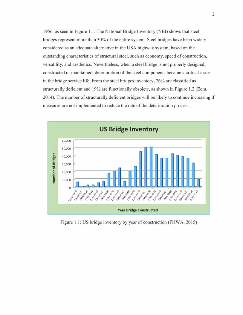
1956, as seen in Figure 1.1. The National Bridge Inventory (NBI) shows that steel
bridges represent more than 30% of the entire system. Steel bridges have been widely
considered as an adequate alternative in the USA highway system, based on the
outstanding characteristics of structural steel, such as economy, speed of construction,
versatility, and aesthetics. Nevertheless, when a steel bridge is not properly designed,
constructed or maintained, deterioration of the steel components became a critical issue
in the bridge service life. From the steel bridges inventory, 26% are classified as
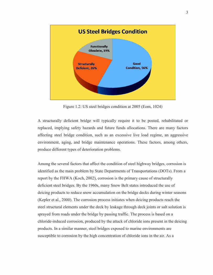
structurally deficient and 19% are functionally obsolete, as shown in Figure 1.2 (Eom,
2014). The number of structurally deficient bridges will be likely to continue increasing if
measures are not implemented to reduce the rate of the deterioration process.
Figure 1.1: US bridge inventory by year of construction (FHWA, 2015)
0
10,000
20,000
30,000
40,000
50,000
60,000
Nu
mb
er
of
Bri
dg
es
Year Bridge Constructed
US Bridge Inventory
3
Figure 1.2: US steel bridges condition at 2005 (Eom, 1024)
A structurally deficient bridge will typically require it to be posted, rehabilitated or
replaced, implying safety hazards and future funds allocations. There are many factors
affecting steel bridge condition, such as an excessive live load regime, an aggressive
environment, aging, and bridge maintenance operations. These factors, among others,
produce different types of deterioration problems.
Among the several factors that affect the condition of steel highway bridges, corrosion is
identified as the main problem by State Departments of Transportations (DOTs). From a
report by the FHWA (Koch, 2002), corrosion is the primary cause of structurally
deficient steel bridges. By the 1960s, many Snow Belt states introduced the use of
deicing products to reduce snow accumulation on the bridge decks during winter seasons
(Kepler et al., 2000). The corrosion process initiates when deicing products reach the
steel structural elements under the deck by leakage through deck joints or salt solution is
sprayed from roads under the bridge by passing traffic. The process is based on a
chloride-induced corrosion, produced by the attack of chloride ions present in the deicing
products. In a similar manner, steel bridges exposed to marine environments are
susceptible to corrosion by the high concentration of chloride ions in the air. As a
4
consequence of corrosion, a structural steel member loses part of its mass and section
thickness, causing it to be susceptible to partial failure of the member or the total collapse
of the structural system.
Bridge preservation can be defined as the ability to keep a bridge structure in good
condition as long as possible, thereby slowing the process of deterioration. Bridge
preservation can be achieved through the performance of some selected bridge
maintenance activities, at some regular frequency and following appropriate practices. It
has been shown in different studies that a program of low cost maintenance activities,
performed with some regular frequency, is a cost-effective practice, instead of
performing few expensive bridge repairs, rehabilitations or even replacements, during the
bridge service life (Hopwood, 1999; Purvis, 2003; NYSDOT, 2008; Spuler et al, 2012).
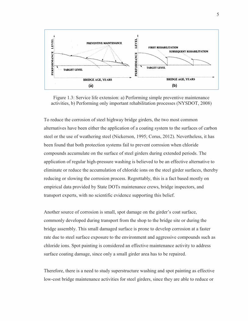
Figure 1.3 depicts the performance level for a bridge under two different programs: one
considering a maintenance program with frequent low-cost activities, versus a program
with no maintenance considerations but the performance of a few expensive
rehabilitations.
Life-cycle cost analysis (LCCA) is an efficient tool to analyze and select the best
alternative from different options (Hawk, 2003; Azizinamini et al., 2013). The
application of LCCA has proven that performing frequently low-cost bridge maintenance
alternatives is more cost-effective than alternatives expecting only high-cost
rehabilitations or replacements (Weyers et al., 1993; Chang et al., 1999; RIDOT, 2002).
Consequently, bridge maintenance activities are expected to be an effective alternative to
prolong the bridge service life at a low cost.
5
Figure 1.3: Service life extension: a) Performing simple preventive maintenance
activities, b) Performing only important rehabilitation processes (NYSDOT, 2008)
To reduce the corrosion of steel highway bridge girders, the two most common
alternatives have been either the application of a coating system to the surfaces of carbon
steel or the use of weathering steel (Nickerson, 1995; Corus, 2012). Nevertheless, it has
been found that both protection systems fail to prevent corrosion when chloride
compounds accumulate on the surface of steel girders during extended periods. The
application of regular high-pressure washing is believed to be an effective alternative to
eliminate or reduce the accumulation of chloride ions on the steel girder surfaces, thereby
reducing or slowing the corrosion process. Regrettably, this is a fact based mostly on
empirical data provided by State DOTs maintenance crews, bridge inspectors, and
transport experts, with no scientific evidence supporting this belief.
Another source of corrosion is small, spot damage on the girder’s coat surface,
commonly developed during transport from the shop to the bridge site or during the
bridge assembly. This small damaged surface is prone to develop corrosion at a faster
rate due to steel surface exposure to the environment and aggressive compounds such as
chloride ions. Spot painting is considered an effective maintenance activity to address
surface coating damage, since only a small girder area has to be repaired.
Therefore, there is a need to study superstructure washing and spot painting as effective
low-cost bridge maintenance activities for steel girders, since they are able to reduce or
6
delay the corrosion process. The effectiveness of these activities should be justified by an
economic analysis supported by methods such as the Life Cycle Cost Analysis.
1.3 Objectives of the Research
The objective of this research was to understand, model, and assess the structural
capacity degradation of typical steel girder highway bridges due to the atmospheric
corrosion, so that the benefit of regular high-pressure superstructure washing and spot
painting can be evaluated as effective maintenance activities to reduce the corrosion
process. The effectiveness of steel girder washing was assessed by developing models of
corrosion deterioration of composite steel girders and analyzing steel coupons at the
laboratory under atmospheric corrosion for two alternatives: when high-pressure washing
was performed and when washing was not considered. The effectiveness of spot painting
was assessed by analyzing the corrosion on steel coupons, with small damages,
unprotected and protected by spot painting.
Corrosion models were developed to estimate the loss of mass and reduction of section
thickness with aging. The corrosion models also considered the corrosion penetration
patterns exhibited by typical steel highway bridge girders. A series of accelerated
corrosion laboratory tests were performed on small steel samples to reproduce the effect
of both high-pressure washing and spot painting in reducing the corrosion. From the
accelerated tests a series of curves relating aging time with corrosion penetration were
established.
Based on the section reduction by corrosion, the structural capacity reduction of steel
highway bridge girders was analyzed. The reduction of structural capacity of steel girder
bridges due to environmental corrosion was assessed by performing a parametric study
on typical steel highway bridges of one and two spans, with different span lengths,
different steel types, exposed to different environments, and under different maintenance
alternatives. The structural capacity reduction was estimated by performing a structural
7
analysis on composite steel girder bridge models using a finite element software. The
reduction of bending and shear capacity, and the increment of deflections, were estimated
using the limit state functions given by the AASHTO LRFD Bridge Design
Specifications (AASHTO, 2012), and performing the bridge load rating based on
specifications from the Manual for Bridge Evaluation (AASHTO, 2011).
1.4 Scope of the Research
Steel corrosion is a complex problem due to the influence of several factors, all of them
with significant variations and uncertainties involved during the process. Corrosion is a
combination of physical and chemical processes that requires considerable time to be
developed, sometimes months or even years, according to the surrounding atmospheric
conditions and steel properties. This study was limited to consider the effect of uniform
corrosion as the only factor for structural degradation of the steel highway bridge girders.
The atmospheric corrosion was studied considering three macro-environments:
Industrial/Urban, Marine, and Rural. The analyzed girders were constructed from carbon
steel and weathering steel, both uncoated and coated using a three-layer system
(inorganic zinc primer, epoxy intermediate coat and a polyurethane finish coat). The
structural analysis considered typical steel girder highway bridges, of one and two spans.
The following tasks were performed to achieve the objective of this research:
· Perform a literature review of studies related to steel corrosion process in general,
corrosion processes on steel girder highway bridges, accelerated corrosion tests,
structural analysis of corroded steel girder bridges, bridge load rating process, bridge
maintenance activities, high-pressure washing/flushing of steel girder, spot painting,
and cost/benefit analysis.
· Implement an accelerated corrosion process to replicate corrosion degradation of steel
samples in the laboratory.
· Develop a set of experimental curves to relate the frequency of high-pressure washing
treatments with corrosion rates at different typical environments.

8
· Identify a corrosion rate model based on reliable documented experiences to be
related with curves of corrosion rates obtained from laboratory tests.
· Analyze the effect of spot painting on scribed plates.
· Define typical steel girder highway bridge models of one and two spans, of different
span lengths, and for different types of steel, to be analyzed under different levels of
corrosion.
· Study the loss of structural capacity and serviceability of steel highway bridges with
time due to general corrosion effects.
· Evaluate the cost/benefit ratio for two alternatives: when steel girders are treated with
high-pressure washing to reduce the corrosion process and when washing is not
performed.
· Propose an efficient frequency for periodic washing/flushing maintenance activities
that minimize the loss of structural capacity of steel bridges due to corrosion and
maximize the allocated resources.

9
LITERATURE REVIEW
Part of this research was a review of relevant literature on corrosion of steel beam and
girder highway bridges, maintenance activities for steel highway bridges, accelerated
corrosion tests, and structural analysis, design, and load rating of corroded steel highway
bridges. Abundant literature and research on steel corrosion was found; limited
information on atmospheric corrosion of steel highway bridges was located; and very few
documents were found on the effectiveness of bridge maintenance activities in reducing
the rate of atmospheric corrosion of steel girders.
2.1 Research on Atmospheric Corrosion of Steel Girder Highway Bridges
According to Czarnecki (2006) steel bridges deteriorate during their service life due to
several effects, with the most influential involving the surrounding environment, changes
in live loads, and structural fatigue. Size and capacity of modern trucks have increased in
the last few decades, requiring greater bridge resistant capacities. Evaluation of bridge
capacities focuses on structure and material capacities and resistances. Steel highway
bridge design requires special considerations with respect to material degradation due to
environmental effects, especially atmospheric corrosion attack. The resistances of steel
bridge members change in time due to environmental attack (Kayser, 1988; Czarnecki,
2006; Rahgozar, 2009).
In the National Cooperative Highway Research Program Report 272, Albrecht and
Naeemi (1984) studied the performance of weathering steel in bridges, and also the
performance for other steel types, such as carbon steel and copper steel. The main
10
concern in this study was atmospheric corrosion attack, their causes, consequences, and
alternatives to reduce the problems. The document emphasizes the influence of the
environment surrounding the bridge as the main factor for corrosion degradation. The
study by Albrecht and Naeemi (1988) indicated that the use of deicing salts is one of the
leading causes of corrosion in steel bridge members. They mentioned that especially in
the “snow belt” states of the USA, steel bridges are exposed to corrosion attack due to
contamination from deicing salt compounds in different ways. Albrecht and Naeemi
(1984), Kayser (1988), and Czarnecki (2006) mentioned that debris accumulation on the
horizontal surfaces of steel members is another source for corrosion attack since they are
able to retain moisture, chloride and sulfate compounds in contact with the steel surface
for a prolong period of time. In the same sense, Kogler (2012) indicated that the time of
wetness is an issue for steel bridge member areas that trap or retain water or debris. “The
severity of the deterioration depends upon how much water gets to the steel and how long
it remains there (Kayser, 1988).” Morcillo (2011) indicated that steel bridge members
will corrode at different rates during their exposure in different environments.
Corrosion is developed in several forms in steel bridge members. General (uniform)
corrosion is the most common, causing gradual reduction in section thicknesses
(Rahgozar, 2009). For instance, the Michigan DOT investigated the corrosion of steel
bridges in the state of Michigan (McCrum et al., 1985). The study found a rate of uniform
corrosion at exposed surfaces that ranged from 0.2 mils per year to 6 mils per year. In the
same study it was reported that pitting corrosion in shielded areas can be as high as 16
mils per year. The estimation of steel loss of thickness from atmospheric corrosion has
been a serious concern and several models have been developed.
Various corrosion models, developed from different approaches, can be classified as first
level and second level models. First level models are based on the relationships from the
steel and microenvironment components and the application of laws from physics and
chemistry. The second level models are oriented to engineering applications and estimate
the corrosion penetration from the loss of mass with time (Landolfo et al., 2010). Due to
11
the most direct application to the solution of engineering problems, the second level
models were used in this study.
Townsend and Zoccola (1982) found that corrosion penetration results, obtained from
atmospheric tests, were well predicted using a power function of the form C = AtB. In this
expression, C is the corrosion penetration, t is the exposure time, and A and B are
constants. McCuen and Albrecht (1994) recommended a composite power-lineal model
that consisted of two expressions, the first a power function similar to that from
Townsend and Zoccola and the second a linear expression. McCuen and Albrecht (1994)
also presented a composite power-power model, comprised of two power equations to
describe the corrosion penetration in time.
To consider the delay of corrosion initiation, due to coating protection, Park et al. (1998)
presented a modified corrosion model, with near zero corrosion for the first fifteen to
twenty years, until the paint or protective cover deteriorates and then corrosion damage
starts to develop. From several studies (Kayser, 1988; Park et al., 1998; Czarnecki, 2006)
there is an agreement that steel girders corrode at higher rates at the upper face of the
bottom flange along all the span, over the entire web near the supports, and at the lower
portion of the web away from the supports.
The main effects of atmospheric corrosion on steel bridge members have been identified
by many researchers. Those effects are mostly linked to degradation of the bridge safety,
capacity, and serviceability (Kayser and Nowak, 1989; Park et al., 1998; Czarnecki,
2006; Rahgozar, 2009). Rahgozar (2009) pointed out that loss of material due to
corrosion produces a change in the section properties of a steel member (area, moment of
inertia, radius of gyration, etc.), hence causing a reduction in the member carrying
capacity, and therefore, reducing the entire structural capacity. Park et al. (1998)
indicated that steel girder corrosion may affect the bridge resistant capacity in bending,
shear and bearing.
12
2.2 Research in Bridge Maintenance Activities
Appropriate bridge maintenance activities can prolong the bridge service life at relative
low costs if they are routinely conducted (FHWA, 2011). The necessity for effective
bridge maintenance treatments is widely recognized, but they are often limited by
constrained allocations (Kim 2005). There are several maintenance activities recognized
by State DOTs and federal agencies as effective alternatives to reduce the corrosion on
steel highway bridges (MnDOT, 2006; NYSDOT, 2008; MDOT, 2010; FHWA, 2011).
Ford et al. (2012) referenced the work by Sinha et al. (2009), who indicated that the
service life of a bridge in Indiana could vary between 35 to 80 years based on the
program of maintenance/preservation activities provided for the bridge. Effective
inspections and appropriate maintenance activities are required to ensure a bridge will
reach its expected service life (ITD, 2008). Czarnecki (2006) indicated that “if a steel
highway bridge is not maintained properly (regular cleaning, inspection, repainting, and
repair) steel corrosion occurs.”
In 1988 the Federal Highway Administration sponsored a Weathering Steel Forum, with
specialists from throughout the US (FHWA, 1989). The speakers presented histories and
data from studies on the use of weathering steel in highway structures. As a result of the
event, suggested guidelines were presented as recommendations to achieve the greatest
potential of the product. One of the recommendations from the guidelines was focused on
maintenance actions, indicating that “effective inspection and maintenance programs are
essential to ensure that all bridges reach their intended service life. This is especially true
in the case of uncoated weathering steel bridges” (FHWA, 1989). Some specific
maintenance activities recommended by the document were: “Remove dirt, debris and
other deposits that hold moisture and maintain a wet surface condition on the steel. In some
situations, hosing down a bridge to remove debris and contaminants may be practical and
effective. Some agencies have a regularly scheduled program to hose down their bridges”.
13
A study from the Rhode Island Department of Transportation (RIDOT, 2002) analyzed
the effectiveness of washing Interstate highway bridges. The analysis was done applying
PONTIS (Golabi et al., 1993), a bridge management software developed by AASHTO, to
a random sample of 96 steel bridges from the state inventory. PONTIS utilizes
mathematical formulas and probability estimates to predict future bridge conditions,
based on current condition and the application of hypothetical actions on the structure. In
this case, an eight years period (arbitrary) was considered as a framework for two
alternatives. One alternative was the “Do Nothing" (DN) alternative during the eight
years period, while the other alternative was the implementation of a regular bridge
cleaning and washing program, performed each two years during the eight years. The
PONTIS element No. 107 “Painted steel open girder” was utilized for the analysis. The
PONTIS program classifies the condition of a “Painted steel open girder” in a five levels
scale (1 to 5). Based on transitional probabilities, the study assumed the percentages of
probability that one element remains on its current state or decreases one level when
nothing is done to protect it. On the other hand, there is a 100% (certainty) that an
element in conditions 1 or 2 will remain in its current condition when using a regular
washing program. After applying the transitional probabilities to the selected bridges,
each two years for a period of eight years, the predicted conditions of the bridges were
obtained for both alternatives. An economic analysis for the total cost of both alternatives
showed that providing a regular maintenance program to a painted steel open girder,
consisting of cleaning and washing, would be more cost-effective than the Do Nothing
alternative.
The Shikoku Regional Bureau of Japan Highway Public Co. (JH) conducted a pilot study
from 2001 to 2004 based on the behavior of two weathering steel bridges under an
experimental bridge washing program (Hara et al., 2005). The focus of the study was to
analyze the effect of bridge superstructure washing as a mean to eliminate corrosive
products derived from deicers applied on bridge decks. During the study fixed points on
the bridge girders were observed and documented once a year, before and after the
application of deicers products. For those points in the steel surface the loss of mass and
14
rust characteristics were analyzed. The researchers concluded that washing the steel surface
had the effect of suppressing the increase of rust particles size, and this was a way to reduce
the corrosion due to deicer products.
The Iowa Department of Transportation (Iowa DOT) together with Wiss, Janney, Elsner
Associates, Inc. (WJE), studied the behavior of steel weathering bridge structures
(Crampton et al., 2013). The research considered methods to assess the quality of the
weathering steel patina layer and chloride contamination, and the possible benefits from
regular bridge washing. The study concluded that high-pressure washing (3,500 psi) is an
adequate procedure to reduce chloride ion concentrations on weathering steel patinas;
however, not all chlorides could be completely eliminated. This could indicate that bridge
superstructure washing mainly removes chlorides from the patina surface, while some
amount of chlorides remains under the patina surface, inside the pores and voids of the
patina. WJE found that when performed immediately after the winter deicing season,
bridge washing will be able to remove the majority of chloride products, before they
migrate under the patina layer, as predicted by Fick’s Law. Therefore, the study concluded
that repeating bridge washing on a regular basis will reduce the corrosion process on the
steel girders, but qualified this conclusion and indicated that further study needs to be
conducted on this topic.
A study sponsored by the Washington State Department of Transportation (WSDOT) and
the Federal Highway Administration (FHWA) analyzed the costs and benefits of regular
washing of steel bridges (Berman et al., 2013). The study was implemented in 2011,
consisting in washing some bridges annually while some other would not be washed.
WSDOT inspectors will annually inspect each bridge from the project and will record steel
coating condition and corrosion level, for both, washed and unwashed bridges. Processing
the data obtained annually will indicate the cost effectiveness of bridge washing for
extending steel coating life and retarding the corrosion process. The project is at present
under development. As part of the study, Berman et al. (2013) conducted a national survey
15
to all DOT agencies, reporting that seven State DOTs agencies performed some type of
steel bridge washing on a regular basis.
2.3 Research on Accelerated Corrosion Tests
Accelerated corrosion tests are used with the aim to produce atmospheric corrosion in the
laboratory in a greatly reduced time (Guthrie, 2002; Lin, 2005). There are three main
types of corrosion tests according to Guthrie (2002): service testing, field testing, and
laboratory testing. Service testing is the most reliable since it provides actual results from
the actual in situ corrosion processes. Regrettably, the results from service tests are
limited to the period of time the test lasts, which normally is far too short to achieve
useful results. Field tests also offer excellent results on reproducing corrosion but they
have the same limitations as service tests. Hence, accelerated corrosion tests are an
adequate alternative to achieve appropriate results in a very short period of time (Guthrie,
2002). The results from accelerated tests are always an approximation to reality and they
are only as good as the laboratory conditions approached the service conditions
(Carlsson, 2006).
At the moment there are several standard procedures to perform accelerated corrosion
tests, with most of them developed for the coating automotive industry. “The oldest and
most widely used method for laboratory accelerated corrosion testing is the continuous
neutral salt spray test (Carlsson, 2006).” Originally published in 1939, the ASTM B117
procedure has been used for many years as an accelerated corrosion test for all types of
applications (Cremer, 1996). Since corrosion processes include several variations, other
standardized accelerated tests have been developed and implemented, with the aim to
approach certain specific corrosion characteristics (Guthrie, 2002).
Given the several assumptions established during accelerated corrosion tests, the results
have to be accepted with an adequate margin of error. Lin (2005) applied the ASTM
B117 standard to perform an accelerated corrosion tests to study three types of steel: soft

16
steel (hot rolled), carbon steel, and weathering steel. The research objective was to
establish a correlation between corrosion rates and corrosion factors such as chloride
deposition fluxes, time of wetness, and temperature at real environments. Measuring the
weight loss from specimens at real environment and in the laboratory, Lin (2005)
established the correlations between predicted and measured thickness loses due to
atmospheric corrosion. The results from the study showed the following margin of errors:
for soft steel 29.0%, carbon steel 28.7%, and weathering steel 37.2%. Clearly, some
degree of error always exists when an accelerated test is used to model corrosion.
2.4 Research on Structural Analysis and Design of Corroded Composite Steel Girders
Several studies in relation to the structural analysis and design of steel girder bridges
under the effects of atmospheric corrosion attack have been conducted. All those studies
had to define several parameters and model some structural characteristics, such as: the
types of corrosion affecting the steel superstructure, the rate of corrosion penetration with
time, identify the steel member zones where corrosion develops, define appropriate limit
state functions, specify load and resistant models, and identify the effects of corrosion
attack to structural members and to structural systems (Kayser, 1988; Park, 1999;
Czarnecki, 2006). In general, the studies analyzed the corrosion progression on structural
steel members and its effect on the structural capacity and serviceability of the bridge
system.
Kayser (1988) studied the effect of atmospheric corrosion on typical steel girder highway
bridges. The study examined four, single span, composite steel girder bridges. The bridge
spans ranged from 40 ft. to 100 ft. with increments of 20 ft. The superstructure comprised
a concrete deck supported by five steel A36 girders, carrying two traffic lanes. The study
by Kayser (1988) focused on the structural deterioration in an unprotected marine
environment for a service life of fifty years. The study concluded that: 1) the environment
surrounding the bridge has a significant influence on the deterioration of safety and
capacity, 2) corrosion affects the bending, shear, and bearing resistance of the structure,
17
3) a reduction of the bridge resistance (bending, shear, and bearing) occurs at different
rates, changing the original bridge configuration.
Park (1999) implemented a series of structural analyses on typical steel girder highway
bridges to investigate the effect of corrosion on composite steel girders. The analysis
included the variation of several parameters, such as: span length, deck thickness, number
of girders, girder spacing, and degree of corrosion. The research performed a parametric
analysis for a service life of 120 years. From his research, Park (1999) observed that
corroded steel girders are more affected in their shear capacity than their bending
capacity. This conclusion was justified due to the thickness reduction of the web. Shear
buckling on steel girders was found as the governing failure mode at the end of the bridge
service life.
The research performed by Czarnecki (2006) evaluated composite steel girder bridges
under atmospheric corrosion. The study comprised the analysis of fifty-four, single span,
typical steel highway bridges. The study took into account the variation of span length,
number of steel girders, girder spacing, type of environment, and load carrying capacity.
Czarnecki (2006) concluded that corroded steel girders produce a reduction in the
structure strength capacity, increasing the probability of failure. The study also showed
that the bridge resistance capacity is reduced in larger proportion in shorter spans than for
longer spans.
18
CORROSION OF STEEL BRIDGE HIGHWAY GIRDERS
3.1 Introduction
Corrosion is one of the most significant problems a highway system must confront. Steel
girder bridges are crucial components of any highway system and they are constantly
threated by exposure to aggressive environments. To establish adequate, practical, and
economical solutions, it is necessary to understand how corrosion develops on structural
steel bridge members. Understanding the cause of corrosion and the problems corrosion
generates are basic requirements to propose solution alternatives for existing bridges.
This chapter presents a review of those causes and problems of corrosion on steel girders.
Also, some mathematical models are proposed to predict the amount of corrosion
penetration and the location in the steel girder where corrosion takes place.
3.2 Structural Steel
3.2.1 Characteristics of Structural Steel
Structural steel is a product extensively used in the construction of buildings, bridges,
factories, and many other structures. Steel used in construction typically conforms to
specific standard specifications such as sections dimensions, chemical composition, and
physical and mechanical properties. Structural steel is mainly composed of a combination
of iron (Fe), carbon (C), and manganese (Mn). The addition of extra constituents
(chromium, copper, etc.) as alloy elements, enhances certain steel capabilities, for
example higher strength, higher corrosion resistance, etc. Carbon is the element

19
responsible for steel resistance; however, an excessive content of carbon reduces other
important steel properties, such as toughness and weldability (Barker and Puckett, 2007).
Structural steel is recognized as an advantageous construction material due to its
controlled production, light weight, and rapid on-site assembly. Also, structural steel is
the most recyclable construction material, since more than 93% of structural steel in the
USA is produced from recycled steel scrap (AISC, 2015).
Structural steel used in steel bridge construction is exposed to more stringent conditions
than steel used for buildings or other structural facilities. Steel bridges require special
capabilities to support exposure to: aggressive environments, fatigue under millions of
load-unload cycles, daily strong temperature changes, and corrosive compounds from
deicing products (FHWA, 2012). Consequently, the structural steel material and
environmental requirements for bridges are more rigorous than those for general
structural steel.
Both, the American Association of State Highway Transportation Officials (AASHTO)
and the American Society for Testing and Materials (ASTM) publish structural steel
standards for bridges. The AASHTO specifications for structural steel for bridges are
presented as standards M 270(US units) and M 270M(metric units), while the ASTM
specifications are given in the standards A 709(US units) and A 709M(metric units). The
standards from both organizations are quite similar, with very few differences. Most State
DOTs agencies require that steel bridge design and construction adheres to AASHTO
standard specifications, and are often supplemented with ASTM requirements.
A typical structural steel is best represented by its stress-strain curve, as shown in Figure
3.1. The steel’s modulus of elasticity (Young’s modulus) is defined by the slope of the
elastic part of the stress-strain curve. A conservative value for this modulus is specified to
E = 29,000 ksi (200 GPa), while the yield strength Fy is defined by the 0.2% offset line
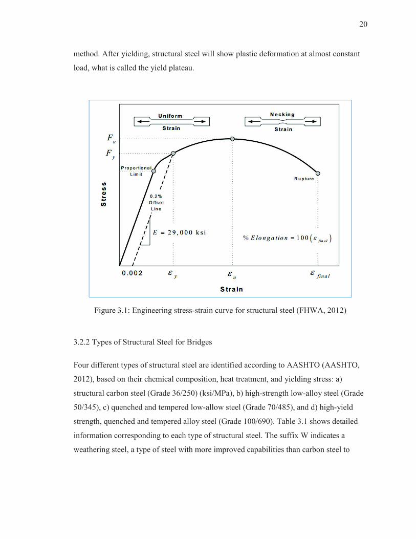
20
method. After yielding, structural steel will show plastic deformation at almost constant
load, what is called the yield plateau.
Figure 3.1: Engineering stress-strain curve for structural steel (FHWA, 2012)
3.2.2 Types of Structural Steel for Bridges
Four different types of structural steel are identified according to AASHTO (AASHTO,
2012), based on their chemical composition, heat treatment, and yielding stress: a)
structural carbon steel (Grade 36/250) (ksi/MPa), b) high-strength low-alloy steel (Grade
50/345), c) quenched and tempered low-allow steel (Grade 70/485), and d) high-yield
strength, quenched and tempered alloy steel (Grade 100/690). Table 3.1 shows detailed
information corresponding to each type of structural steel. The suffix W indicates a
weathering steel, a type of steel with more improved capabilities than carbon steel to
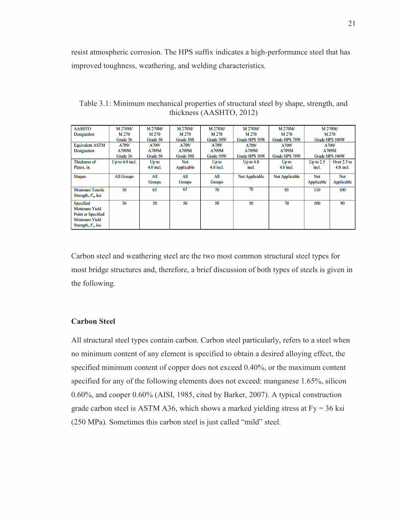
21
resist atmospheric corrosion. The HPS suffix indicates a high-performance steel that has
improved toughness, weathering, and welding characteristics.
Table 3.1: Minimum mechanical properties of structural steel by shape, strength, and
thickness (AASHTO, 2012)
Carbon steel and weathering steel are the two most common structural steel types for
most bridge structures and, therefore, a brief discussion of both types of steels is given in
the following.
Carbon Steel
All structural steel types contain carbon. Carbon steel particularly, refers to a steel when
no minimum content of any element is specified to obtain a desired alloying effect, the
specified minimum content of copper does not exceed 0.40%, or the maximum content
specified for any of the following elements does not exceed: manganese 1.65%, silicon
0.60%, and cooper 0.60% (AISI, 1985, cited by Barker, 2007). A typical construction
grade carbon steel is ASTM A36, which shows a marked yielding stress at Fy = 36 ksi
(250 MPa). Sometimes this carbon steel is just called “mild” steel.
22
When carbon steel is exposed to moisture and oxygen, a loose rust surface is formed,
which allows more water and air accumulation, producing more rust and weakening the
steel surface (McDad, 2000). When used for steel bridges, carbon steel must be protected
with a coating system to resist corrosion attack from aggressive environments.
Weathering Steel
Weathering steel is typically a high-strength low-alloy steel which contains 2 percent or
less of alloying components such as copper, phosphorus, chromium, nickel, and silicon
(Albrecht and Naeemi, 1984). In its bare, mature state, weathering steel in contact with
moisture and oxygen is able to develop a dense and adherent oxide film known as
“patina”, which seals the base metal and acts as a protective coat to minimize further
atmospheric corrosion (McDad, 2000). The characteristics of this protective film is a
function of several factors, such as steel age, degree of exposure, and environment
conditions. When properly specified, weathering steel can provide an alternative to
reduce the maintenance cost of bridge painting.
To form its protective film weathering steel needs to be exposed to environments with
continuous wet-dry cycles and free of an atmosphere with salt contents. Otherwise, when
exposed to prolong periods of wetness and high levels of deicing salts, weathering steel
will corrode as plain carbon steel (Albrecht and Naeemi, 1984).
3.3 Corrosion of Structural Steel
3.3.1 Definition of Corrosion
The word corrosion is derived from the Latin corrosus which means eaten away or
consumed by degrees (Syed, 2006). Corrosion is defined as the degradation of a material
by interaction with its surrounded environment (Jones, 1996). The corrosion process is
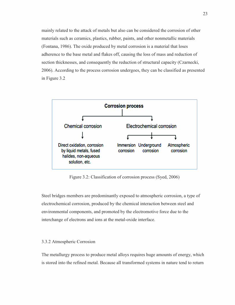
23
mainly related to the attack of metals but also can be considered the corrosion of other
materials such as ceramics, plastics, rubber, paints, and other nonmetallic materials
(Fontana, 1986). The oxide produced by metal corrosion is a material that loses
adherence to the base metal and flakes off, causing the loss of mass and reduction of
section thicknesses, and consequently the reduction of structural capacity (Czarnecki,
2006). According to the process corrosion undergoes, they can be classified as presented
in Figure 3.2
Figure 3.2: Classification of corrosion process (Syed, 2006)
Steel bridges members are predominantly exposed to atmospheric corrosion, a type of
electrochemical corrosion, produced by the chemical interaction between steel and
environmental components, and promoted by the electromotive force due to the
interchange of electrons and ions at the metal-oxide interface.
3.3.2 Atmospheric Corrosion
The metallurgy process to produce metal alloys requires huge amounts of energy, which
is stored into the refined metal. Because all transformed systems in nature tend to return
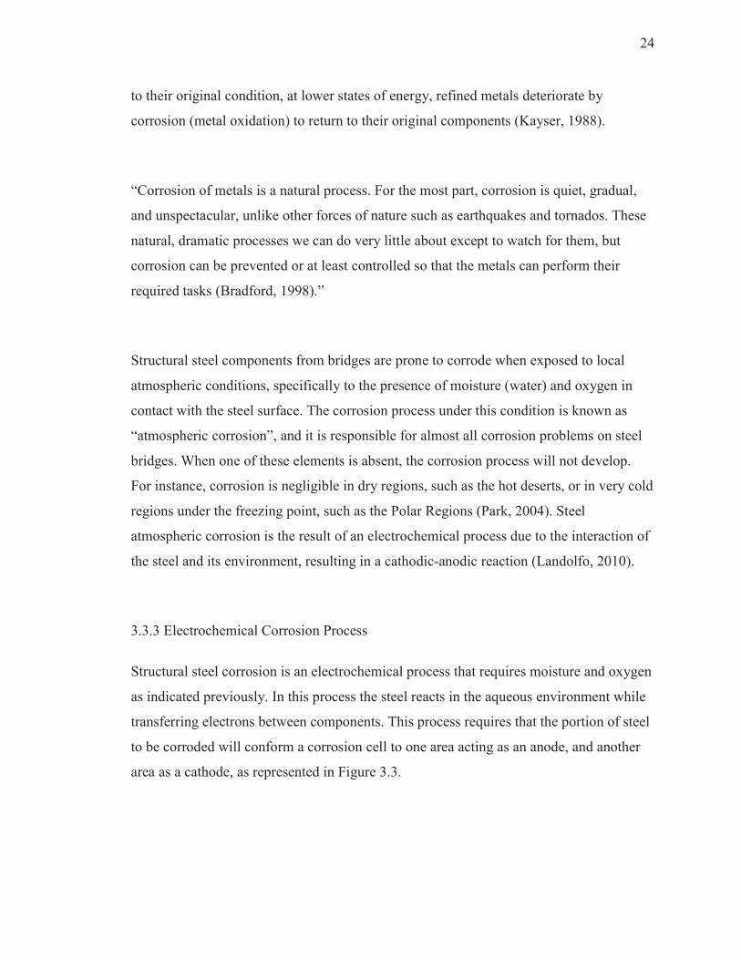
24
to their original condition, at lower states of energy, refined metals deteriorate by
corrosion (metal oxidation) to return to their original components (Kayser, 1988).
“Corrosion of metals is a natural process. For the most part, corrosion is quiet, gradual,
and unspectacular, unlike other forces of nature such as earthquakes and tornados. These
natural, dramatic processes we can do very little about except to watch for them, but
corrosion can be prevented or at least controlled so that the metals can perform their
required tasks (Bradford, 1998).”
Structural steel components from bridges are prone to corrode when exposed to local
atmospheric conditions, specifically to the presence of moisture (water) and oxygen in
contact with the steel surface. The corrosion process under this condition is known as
“atmospheric corrosion”, and it is responsible for almost all corrosion problems on steel
bridges. When one of these elements is absent, the corrosion process will not develop.
For instance, corrosion is negligible in dry regions, such as the hot deserts, or in very cold
regions under the freezing point, such as the Polar Regions (Park, 2004). Steel
atmospheric corrosion is the result of an electrochemical process due to the interaction of
the steel and its environment, resulting in a cathodic-anodic reaction (Landolfo, 2010).
3.3.3 Electrochemical Corrosion Process
Structural steel corrosion is an electrochemical process that requires moisture and oxygen
as indicated previously. In this process the steel reacts in the aqueous environment while
transferring electrons between components. This process requires that the portion of steel
to be corroded will conform a corrosion cell to one area acting as an anode, and another
area as a cathode, as represented in Figure 3.3.
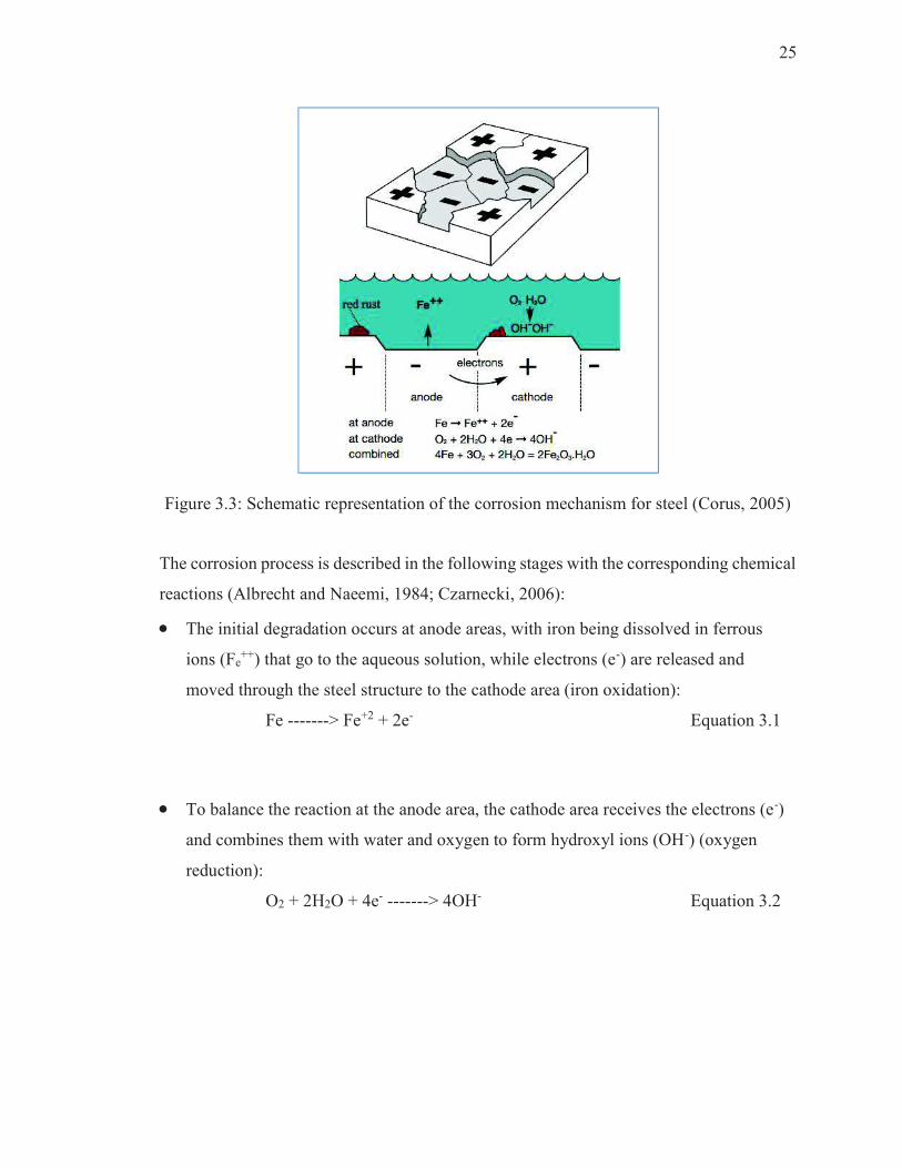
25
Figure 3.3: Schematic representation of the corrosion mechanism for steel (Corus, 2005)
The corrosion process is described in the following stages with the corresponding chemical
reactions (Albrecht and Naeemi, 1984; Czarnecki, 2006):
· The initial degradation occurs at anode areas, with iron being dissolved in ferrous
ions (Fe++) that go to the aqueous solution, while electrons (e-) are released and
moved through the steel structure to the cathode area (iron oxidation):
Fe -------> Fe+2 + 2e- Equation 3.1
· To balance the reaction at the anode area, the cathode area receives the electrons (e-)
and combines them with water and oxygen to form hydroxyl ions (OH-) (oxygen
reduction):
O2 + 2H2O + 4e- -------> 4OH- Equation 3.2
26
· Those hydroxyl ions (OH-) react in the solution with the ferrous ions (Fe++),
producing ferrous hydroxide Fe(OH)2:
Fe+2 + 2OH- -------> Fe(OH)2 Equation 3.3
· Finally, the fresh ferrous hydroxide is oxidized by air, producing hydrated ferric
oxide, most common known as “red rust”
4Fe + 3O2 + 2H2O -------> 2Fe2O3.H2O Equation 3.4
Due to polarization, corrosion in the anodic area is reduced after some time and then a
new reactive anodic area starts to corrode, replicating the aforementioned process. After a
long period, this corrosion process produces a quasi-uniform loss of mass, known as
general corrosion or uniform corrosion.
The rate of corrosion penetration, which is the amount of thickness that it is lost due to
uniform corrosion, is influenced by several factors, such as the steel composition, the
steel surface homogeneity, the time of wetness (TOW) of the steel surface to be corroded,
and the micro-atmosphere composition as the main factors. The content of pollutants
(sulfurs and chlorides) in the atmosphere surrounding the steel member has significant
influence in the level of corrosion.
3.3.4 Forms of Corrosion
According to Fontana (1986), corrosion attack can be classified into eight forms, based
on the appearance and damage produced on the corroded metal. Based on visual
observations corrosion can be classified as: 1) Uniform or general corrosion. 2) Galvanic
corrosion, 3) Crevice corrosion, 4) Pitting corrosion, 5) Intergranular corrosion,
6) Selective leaching corrosion. 7) Erosion corrosion. 8) Stress corrosion. Other identified
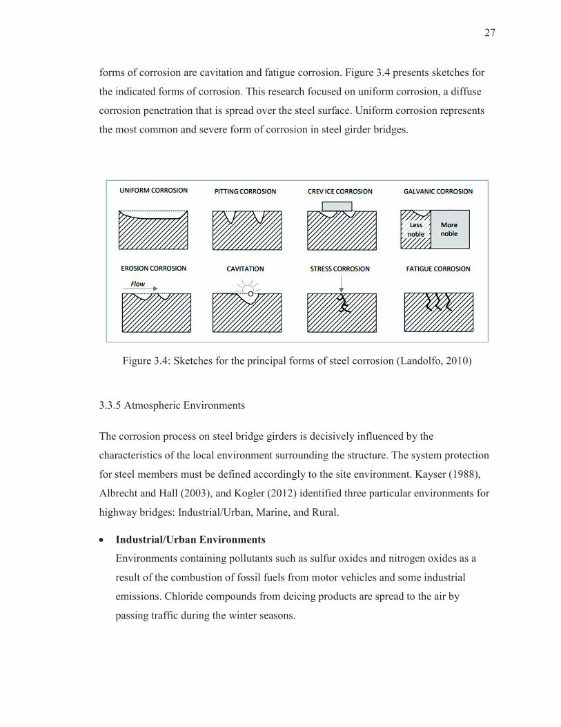
27
forms of corrosion are cavitation and fatigue corrosion. Figure 3.4 presents sketches for
the indicated forms of corrosion. This research focused on uniform corrosion, a diffuse
corrosion penetration that is spread over the steel surface. Uniform corrosion represents
the most common and severe form of corrosion in steel girder bridges.
Figure 3.4: Sketches for the principal forms of steel corrosion (Landolfo, 2010)
3.3.5 Atmospheric Environments
The corrosion process on steel bridge girders is decisively influenced by the
characteristics of the local environment surrounding the structure. The system protection
for steel members must be defined accordingly to the site environment. Kayser (1988),
Albrecht and Hall (2003), and Kogler (2012) identified three particular environments for
highway bridges: Industrial/Urban, Marine, and Rural.
· Industrial/Urban Environments
Environments containing pollutants such as sulfur oxides and nitrogen oxides as a
result of the combustion of fossil fuels from motor vehicles and some industrial
emissions. Chloride compounds from deicing products are spread to the air by
passing traffic during the winter seasons.

28
· Marine Environments
Environments with high contents of salt in the air due to a close proximity to a
seacoast, combined with high levels of humidity and moisture.
· Rural Environments
Environments with a very low rate of pollutants in the air. Their corrosiveness is
produced by moisture, and small compounds of sulfurs and carbon dioxide.
As part of this research, the influence of these three generic environments over steel
girder bridges was analyzed.
3.4 Corrosion of Composite Steel Girders
Corrosion of the structural steel members is one of the most significant factors in
reducing the bridge service life. Steel corrosion could reduce the bridge load-carrying
capacity, and as a consequence, reduce its safety and eventually could collapse during
service. To mitigate or reduce those threats, corrosion should be reduced as much as
possible. To address the reduction of corrosion on steel girders requires a better
understanding of the pattern that the corrosion process follows when attacking a typical
steel girder. The most common causes and problems of steel girder corrosion on typical
highway bridges are presented in the following sections.
3.4.1 Causes of Steel Girder Corrosion
Steel girder bridges commonly involve a reinforced concrete deck supported by steel
girders. The girder and the concrete deck are generally connected by steel shear studs,
forming a composite system. Structural steel corrosion is a time-dependent process. This

29
corrosion process develops with the aging of steel member at a rate depending on the
steel composition, atmospheric characteristics, and bridge maintenance conditions.
Kayser (1988) indicates that a primary cause of corrosion in steel girders is the
accumulation of water on the steel surface, and the rate of corrosion is related to the time
the water remains accumulated. The study identified deck leakage, through damaged
deck joints or deck cracks, as the most common paths for water to reach girders surfaces.
Failure of deck drainage systems is also a very common problem, and as a result,
accumulated water on the deck surface ends flowing through the deck, to the bridge
superstructure elements, including steel girders (Kogler, 2012).
Another way steel girders become wet is due to truck traffic passing under the bridge.
The trucks splash water from the road, creating water plume with sufficient height to wet
the steel girders of the bridge. The corrosion process can be exacerbated during winter
seasons, when deicing products are spread in significant quantities on roads and bridge
decks to facilitate snow and ice removal. The chloride compounds from deicing products
mixed with the water that reaches the steel girder surfaces will significantly increase the
rate of corrosion (Albrecht and Naeemi, 1984).
Debris formations are another source of corrosion problems on steel girders. Debris can
buildup on horizontal surfaces of steel girder and at corners formed by horizontal and
vertical elements. Debris retains moisture, and keep chloride and sulfate compounds in
contact with steel members for a longer period of time, increasing the rate of corrosion on
those areas of contact (Albrecht and Naeemi, 1984; Kogler, 2012).

30
Figure 3.5: Typical corrosion process of steel girders: Left) at the web and bottom flange
(Zaffetti, 2010), Right) Next to a pin and hanger connection (WisDOT, 2011)
Figure 3.6: Debris accumulation at a steel superstructure connection point (Kogler, 2012)
3.4.2 Problems Due to Steel Girder Corrosion
Kulicki et al. (1990) indicates that corrosion can produce four kinds of effects on
structural elements: loss of material, creation of undesired stress concentration,
introduction to unintended fixity, and generation of unintended movements.

31
The loss of material due to corrosion is the most significant effect on structural members
from steel girder bridges because of the reduction in cross section thicknesses. The
reduction of section thicknesses will generate the reduction on the members’ section
properties. Reduction of the area, radius of gyration, and moment of inertia, will thereby
reduce the strength, stiffness and ductility of the corroded structural elements. Under
these conditions, a structural member designed as a particular class of section (plastic,
compact, semi-compact, or slender) may change its conditions, producing stresses not
considered during the design. Hence, the development of the corrosion process could
cause an initial compact section to turn into a semi-compact, or even in a slender section.
These changes will lead to a reduction in the bending, shear, and bearing capacities of the
structural elements, and consequently result in the reduction of both the load-carrying
capacity of the bridge structure and its service capabilities due to larger deflections
(Kayser, 1989, Rahgozar, 2009).
Localized corrosion can also reduce the web thickness of steel girders, introducing new
eccentricities, thus increasing the effect of local buckling, principally near to the
supports. Under millions of cyclic loads as experienced by bridge members, corrosion
can reduce the fatigue strength capacity, especially in zones where high stresses are
concentrated. The buildup of corrosion products can generate changes in the bridge
flexibility, freezing supposed movable parts such as free bearing supports, hinge
connections, or pin-hanger assemblies. These movement restrictions will introduce
undesired stresses into the structural members. Those additional stresses, not considered
during the bridge design, could produce localized damage, or even the failure of a
structural element and possible the total collapse of the bridge. Corrosion products can
also induce unintended movements, affecting some steel members or in occasions the
entire bridge structure (Prucz, 1998; Czarnecki, 2006, Landolfo 2010).
The controlling failure on a corroded structural member can be affected due to corrosion
attack, by reducing its section thicknesses, introducing additional stresses, or changing
32
the original structural configuration. Consequently, the residual capacity of a corroded
member should be evaluated considering all possible modes of failure and verifying their
capacity for strength, stability, serviceability, fatigue and fracture.
3.5 Deterioration Model of Steel Girder Corrosion
To predict the development of corrosion on structural steel bridge members, several
factors have to be taken into account, making the task quite complicated and with a high
degree of uncertainty. The influence of the environment at the bridge location, the
position of steel member within the bridge configuration, the steel composition, and the
presence of sulfurs or chlorides are decisive factors in the corrosion pattern that develops
in a steel member.
Various researchers have developed mathematical models to predict the amount of
corrosion penetration, based on the type of steel and the environment at which the steel
member is exposed (Townsend and Zoccola, 1980; Albrecht and Naeemi, 1984; Komp,
1987). Also, researchers have found that corrosion on steel girders follows some
particular patterns in the steel section and along the span length (Mc Crum et al., 1985;
Kayser, 1988; Kayser and Novak, 1989).
3.5.1 Model to Predict the Rate of Corrosion
There are several studies in relation to models to predict the rate of corrosion penetration
on steel alloys when exposed to different atmospheric conditions (Larrabee and Coburn,
1962; Townsend and Zoccola, 1982; McCuen et Albrecht, 1994). Most of those models
define the rate of corrosion as a function of mass loss or thickness reduction with time.
Generally, the studies are based on the observation of corrosion penetration on steel
coupons exposed to selected atmospheric conditions for certain periods of time,
sometimes months or even years. That limited empirical information is calibrated with
data from laboratory tests and then extrapolated to develop mathematical expressions to
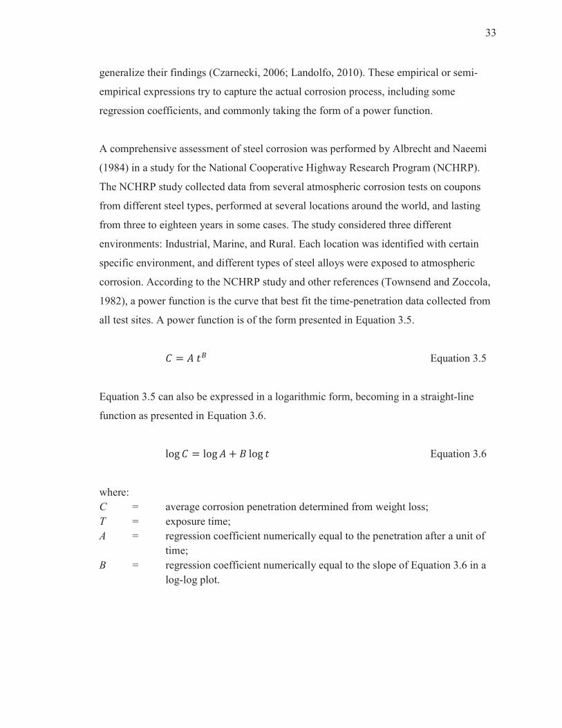
33
generalize their findings (Czarnecki, 2006; Landolfo, 2010). These empirical or semi-
empirical expressions try to capture the actual corrosion process, including some
regression coefficients, and commonly taking the form of a power function.
A comprehensive assessment of steel corrosion was performed by Albrecht and Naeemi
(1984) in a study for the National Cooperative Highway Research Program (NCHRP).
The NCHRP study collected data from several atmospheric corrosion tests on coupons
from different steel types, performed at several locations around the world, and lasting
from three to eighteen years in some cases. The study considered three different
environments: Industrial, Marine, and Rural. Each location was identified with certain
specific environment, and different types of steel alloys were exposed to atmospheric
corrosion. According to the NCHRP study and other references (Townsend and Zoccola,
1982), a power function is the curve that best fit the time-penetration data collected from
all test sites. A power function is of the form presented in Equation 3.5.
� � � �� Equation 3.5
Equation 3.5 can also be expressed in a logarithmic form, becoming in a straight-line
function as presented in Equation 3.6.
log � � log � ! log � Equation 3.6
where:
C = average corrosion penetration determined from weight loss;
T = exposure time;
A = regression coefficient numerically equal to the penetration after a unit of
time;
B = regression coefficient numerically equal to the slope of Equation 3.6 in a
log-log plot.
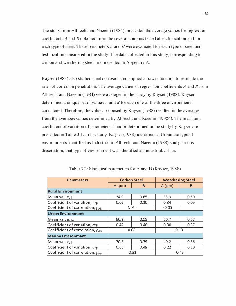
34
The study from Albrecht and Naeemi (1984), presented the average values for regression
coefficients A and B obtained from the several coupons tested at each location and for
each type of steel. These parameters A and B were evaluated for each type of steel and
test location considered in the study. The data collected in this study, corresponding to
carbon and weathering steel, are presented in Appendix A.
Kayser (1988) also studied steel corrosion and applied a power function to estimate the
rates of corrosion penetration. The average values of regression coefficients A and B from
Albrecht and Naeemi (1984) were averaged in the study by Kayser (1988). Kayser
determined a unique set of values A and B for each one of the three environments
considered. Therefore, the values proposed by Kayser (1988) resulted in the averages
from the averages values determined by Albrecht and Naeemi (19984). The mean and
coefficient of variation of parameters A and B determined in the study by Kayser are
presented in Table 3.1. In his study, Kayser (1988) identified as Urban the type of
environments identified as Industrial in Albrecht and Naeemi (1988) study. In this
dissertation, that type of environment was identified as Industrial/Urban.
Table 3.2: Statistical parameters for A and B (Kayser, 1988)
Parameters
A (µm) B A (µm) B
Rural Environment
Mean value, µ 34.0 0.65 33.3 0.50
Coefficient of variation, σ/μ 0.09 0.10 0.34 0.09
Coefficient of correlation, ρAB -0.05
Urban Environment
Mean value, µ 80.2 0.59 50.7 0.57
Coefficient of variation, σ/μ 0.42 0.40 0.30 0.37
Coefficient of correlation, ρAB
Marine Environment
Mean value, µ 70.6 0.79 40.2 0.56
Coefficient of variation, σ/μ 0.66 0.49 0.22 0.10
Coefficient of correlation, ρAB -0.31 -0.45
Carbon Steel Weathering Steel
N.A.
0.190.68

35
Kayser (1988) reported a wide range of variation for parameters A and B between
environments. The same tendency was found for the coefficient of correlation between A
and B. Therefore, Kayser emphasized that corrosion penetration will be approximated
when the A and B are estimated without high confidence. Kayser used the mean values A
and B to extrapolate, the data acquired during Albrecht and Naeemi (1984) tests to 50
years of corrosion penetration values on steel highway bridge girders for the considered
environments. The curves for mean time-corrosion penetration corresponding to carbon
steel when exposed to the three typical environments (Rural, Urban, and Marine) and
projected to 50 years are depicted in Figure 3.7. Actual data colected by Albrecht and
Naeemi (1984) are presented in Figure 3.7 in solid lines, while extrapolated values to 50
years evaluated by Kayser (1988) are presented in dotted lines. Figure 3.7 shows that the
higher corrosion rates are developed at marine environments, followed by rates at urban
environments, and the lower corrosion rates are presented at rural environments. Also,
can be noticed that initial corrosion rates decay in time for the three considered
environments. In Appendix A are presented the complete set of corrosion penetration
curves for the three considered environments.

36
0.00
0.50
1.00
1.50
2.00
0 10 20 30 40 50
Co
rro
sio
n P
en
etr
ati
on
[m
m]
t [years]
CORROSION PENETRATION
CARBON STEEL
Marine
Urban
Rural
Figure 3.7: Mean of Time-Corrosion penetration curves for carbon steel (Kayser, 1988)
Kayser (1988) identified some limitations on his work and had to consider two
assumptions. Firstly, penetration rates obtained using the mean values of parameters A
and B will include certain inaccuracies, due to the high variation found when the
parameters were evaluated. Secondly, some deviations are expected in the corrosion
analysis when the mean values of regression coefficients A and B are used to estimate
actual penetrations on large steel bridge members, since those parameters were obtained
from testing small coupons,
Other authors have presented different penetration models than the power function. Park
et al. (1998) proposed three curves (high, medium, and low) for corrosion penetration
rates. The curves considered initially the steel girders were painted, therefore, the paint
coat provided protection that last the first ten to twenty years, depending on the
environment. The high corrosion rate was assumed for marine environment or heavy
industrial conditions; the low corrosion rate was considered to be developed at dry
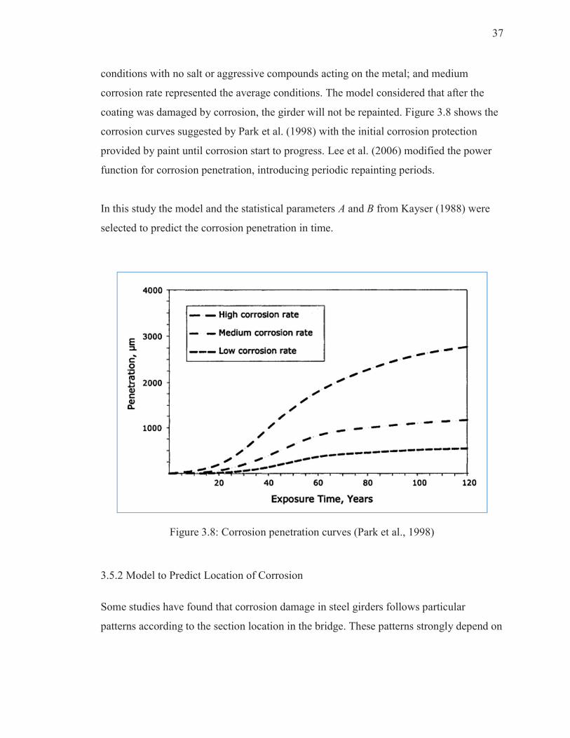
37
conditions with no salt or aggressive compounds acting on the metal; and medium
corrosion rate represented the average conditions. The model considered that after the
coating was damaged by corrosion, the girder will not be repainted. Figure 3.8 shows the
corrosion curves suggested by Park et al. (1998) with the initial corrosion protection
provided by paint until corrosion start to progress. Lee et al. (2006) modified the power
function for corrosion penetration, introducing periodic repainting periods.
In this study the model and the statistical parameters A and B from Kayser (1988) were
selected to predict the corrosion penetration in time.
Figure 3.8: Corrosion penetration curves (Park et al., 1998)
3.5.2 Model to Predict Location of Corrosion
Some studies have found that corrosion damage in steel girders follows particular
patterns according to the section location in the bridge. These patterns strongly depend on
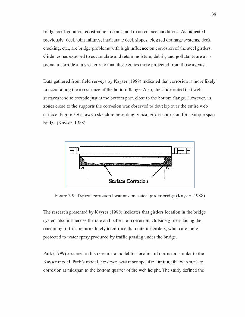
38
bridge configuration, construction details, and maintenance conditions. As indicated
previously, deck joint failures, inadequate deck slopes, clogged drainage systems, deck
cracking, etc., are bridge problems with high influence on corrosion of the steel girders.
Girder zones exposed to accumulate and retain moisture, debris, and pollutants are also
prone to corrode at a greater rate than those zones more protected from those agents.
Data gathered from field surveys by Kayser (1988) indicated that corrosion is more likely
to occur along the top surface of the bottom flange. Also, the study noted that web
surfaces tend to corrode just at the bottom part, close to the bottom flange. However, in
zones close to the supports the corrosion was observed to develop over the entire web
surface. Figure 3.9 shows a sketch representing typical girder corrosion for a simple span
bridge (Kayser, 1988).
Figure 3.9: Typical corrosion locations on a steel girder bridge (Kayser, 1988)
The research presented by Kayser (1988) indicates that girders location in the bridge
system also influences the rate and pattern of corrosion. Outside girders facing the
oncoming traffic are more likely to corrode than interior girders, which are more
protected to water spray produced by traffic passing under the bridge.
Park (1999) assumed in his research a model for location of corrosion similar to the
Kayser model. Park’s model, however, was more specific, limiting the web surface
corrosion at midspan to the bottom quarter of the web height. The study defined the
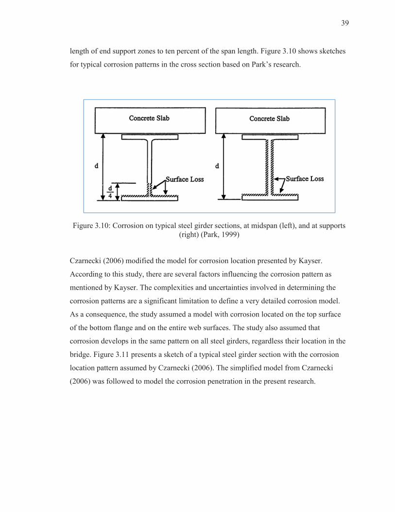
39
length of end support zones to ten percent of the span length. Figure 3.10 shows sketches
for typical corrosion patterns in the cross section based on Park’s research.
Figure 3.10: Corrosion on typical steel girder sections, at midspan (left), and at supports
(right) (Park, 1999)
Czarnecki (2006) modified the model for corrosion location presented by Kayser.
According to this study, there are several factors influencing the corrosion pattern as
mentioned by Kayser. The complexities and uncertainties involved in determining the
corrosion patterns are a significant limitation to define a very detailed corrosion model.
As a consequence, the study assumed a model with corrosion located on the top surface
of the bottom flange and on the entire web surfaces. The study also assumed that
corrosion develops in the same pattern on all steel girders, regardless their location in the
bridge. Figure 3.11 presents a sketch of a typical steel girder section with the corrosion
location pattern assumed by Czarnecki (2006). The simplified model from Czarnecki
(2006) was followed to model the corrosion penetration in the present research.
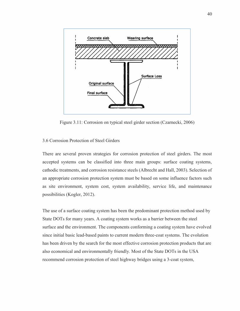
40
Figure 3.11: Corrosion on typical steel girder section (Czarnecki, 2006)
3.6 Corrosion Protection of Steel Girders
There are several proven strategies for corrosion protection of steel girders. The most
accepted systems can be classified into three main groups: surface coating systems,
cathodic treatments, and corrosion resistance steels (Albrecht and Hall, 2003). Selection of
an appropriate corrosion protection system must be based on some influence factors such
as site environment, system cost, system availability, service life, and maintenance
possibilities (Kogler, 2012).
The use of a surface coating system has been the predominant protection method used by
State DOTs for many years. A coating system works as a barrier between the steel
surface and the environment. The components conforming a coating system have evolved
since initial basic lead-based paints to current modern three-coat systems. The evolution
has been driven by the search for the most effective corrosion protection products that are
also economical and environmentally friendly. Most of the State DOTs in the USA
recommend corrosion protection of steel highway bridges using a 3-coat system,
41
consisting of a zinc-rich primer as the main protection coat, combined with an
intermediate epoxy coat, and a finishing urethane topcoat.
The use of weathering steel has also been recommended in the last three decades as an
alternative instead of the use of coating systems to protect steel bridges from corrosion.
As indicated in section 3.2.2, this type of steel produces an adherent film that acts as a
protective coat, allowing the owner to reduce initial costs by mostly eliminating the use
of a coating protection system.
42
MAINTENANCE ACTIVITIES OF STEEL GIRDER BRIDGES
“Preventive maintenance is a planned strategy of cost-effective treatments
to an existing roadway system and their appurtenance that preserves the
system, retards future deterioration, and maintains or improves the
functional condition of the system (without substantially increasing
structural capacity).”
AASHTO Subcommittee on Maintenance (FHWA, 2011)
4.1 Introduction
Department of Transportation agencies need to develop and implement additional
requirements for bridge preservation, rehabilitation, or replacement. According to the
National Bridge Inventory (NBI) 26% of the steel bridge inventory is classified as
structurally deficient and 19% as functionally obsolete (FHWA 2005, cited by Laumet,
2006). The condition of the Indiana highway bridge system is similar to the national
trend. This situation is expected to increase if adequate measures are not implemented,
since appropriate allocations are not enough to solve the entire problem. From the
research by Bowman and Moran (2015), bridge preventive maintenance activities were
analyzed as alternatives to preserve and extend the bridge service life. In that study,
previous studies on bridge preventive maintenance activities were analyzed and
discussed. From that study, several bridge preventive maintenance activities were found
as efficient alternatives to prolong the bridge service life at a low cost. In particular, the
study found that, when properly applied at a regular frequency, bridge superstructure
washing and spot painting are two maintenance activities that are capable of extending
43
the service life of steel girders. Therefore, those activities are viewed as low-cost
alternatives to preserve the bridge serviceability. The objective of the present dissertation
is oriented to study the benefits of these two bridge maintenance activities as alternatives
to enhance corrosion resistance and performance of steel girder bridges. In the next
sections a brief description of these bridge maintenance activities and their benefits are
presented.
4.2 Bridge Superstructure Washing
Steel bridges require an adequate protective system to retard the development of
corrosion attack. In recent years the application of a coating system and/or the use of
weathering steel have been the most common alternatives for corrosion protection (AISI,
1995; Corus, 2012). There are several factors to initiate corrosion attack on steel girders.
Exposure to polluted environments, leaking of deicing compounds from the deck, the
accumulation of dirt, debris, or sand, and water spray produced by moving vehicles are
common sources to initiate the process of corrosion on steel elements (Kayser, 1988;
RIDOT, 2002; Crampton et al., 2013).
Significant corrosion damage of a steel girder due to extended corrosion attack is shown
in Figure 4.1. The loss of section for the extent of corrosion damage shown in Figure 4.1
can compromise the girder strength capability and, in some occasions, the entire bridge
integrity. Consequently, corrosion control is a paramount responsibility for highway
bridge owners.
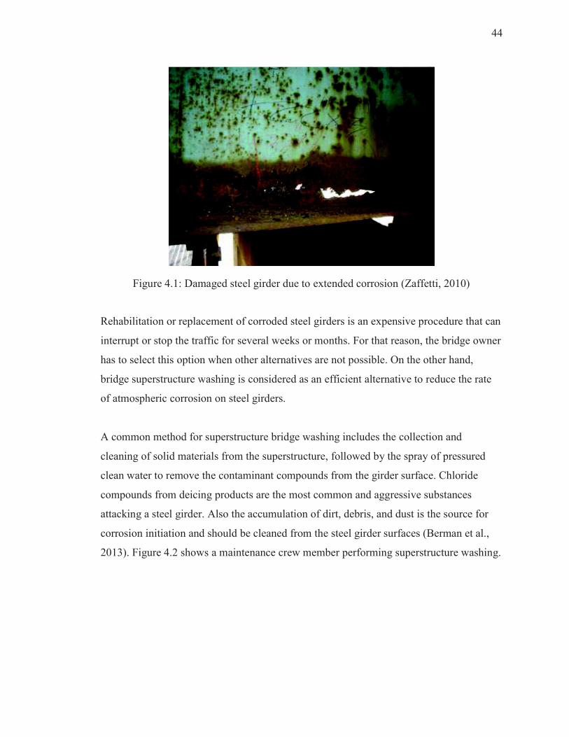
44
Figure 4.1: Damaged steel girder due to extended corrosion (Zaffetti, 2010)
Rehabilitation or replacement of corroded steel girders is an expensive procedure that can
interrupt or stop the traffic for several weeks or months. For that reason, the bridge owner
has to select this option when other alternatives are not possible. On the other hand,
bridge superstructure washing is considered as an efficient alternative to reduce the rate
of atmospheric corrosion on steel girders.
A common method for superstructure bridge washing includes the collection and
cleaning of solid materials from the superstructure, followed by the spray of pressured
clean water to remove the contaminant compounds from the girder surface. Chloride
compounds from deicing products are the most common and aggressive substances
attacking a steel girder. Also the accumulation of dirt, debris, and dust is the source for
corrosion initiation and should be cleaned from the steel girder surfaces (Berman et al.,
2013). Figure 4.2 shows a maintenance crew member performing superstructure washing.
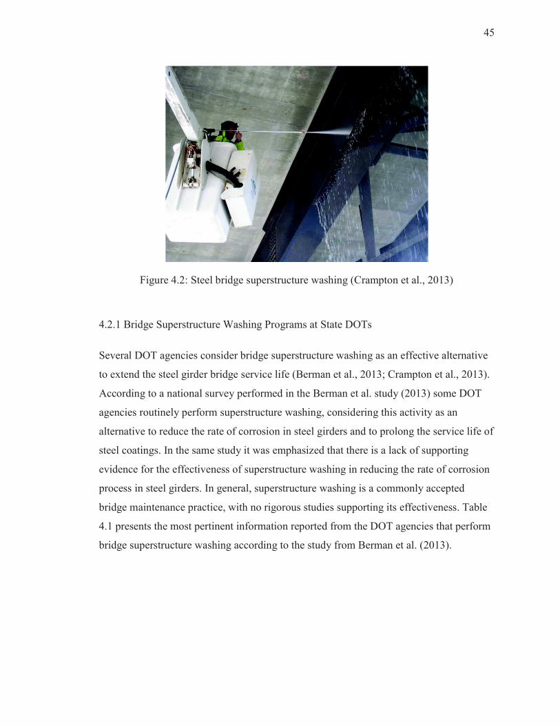
45
Figure 4.2: Steel bridge superstructure washing (Crampton et al., 2013)
4.2.1 Bridge Superstructure Washing Programs at State DOTs
Several DOT agencies consider bridge superstructure washing as an effective alternative
to extend the steel girder bridge service life (Berman et al., 2013; Crampton et al., 2013).
According to a national survey performed in the Berman et al. study (2013) some DOT
agencies routinely perform superstructure washing, considering this activity as an
alternative to reduce the rate of corrosion in steel girders and to prolong the service life of
steel coatings. In the same study it was emphasized that there is a lack of supporting
evidence for the effectiveness of superstructure washing in reducing the rate of corrosion
process in steel girders. In general, superstructure washing is a commonly accepted
bridge maintenance practice, with no rigorous studies supporting its effectiveness. Table
4.1 presents the most pertinent information reported from the DOT agencies that perform
bridge superstructure washing according to the study from Berman et al. (2013).
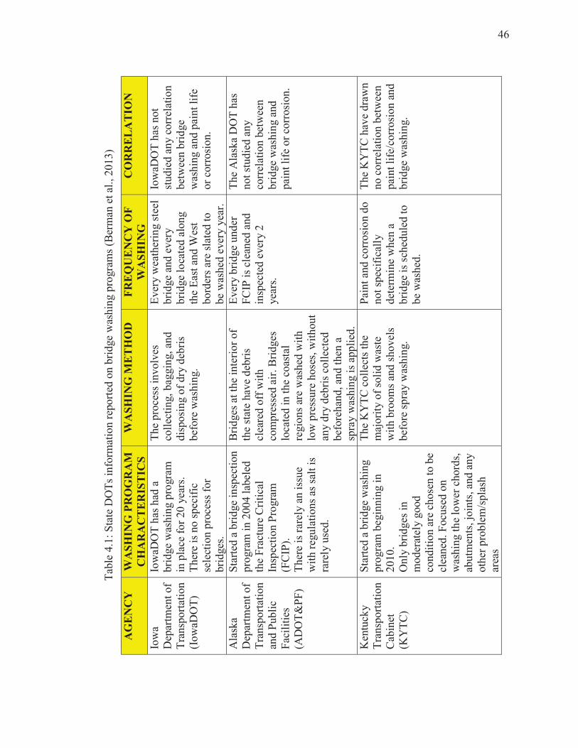
46
Tab
le 4
.1:
Sta
te D
OT
s in
form
atio
n r
epo
rted
on
bri
dge
was
hin
g p
rogra
ms
(Ber
man
et
al.,
20
13
)
AG
EN
CY
W
AS
HIN
G P
RO
GR
AM
CH
AR
AC
TE
RIS
TIC
S
WA
SH
ING
ME
TH
OD
F
RE
QU
EN
CY
OF
WA
SH
ING
CO
RR
EL
AT
ION
Iow
a
Dep
artm
ent
of
Tra
nsp
ort
atio
n
(Io
waD
OT
)
Iow
aDO
T h
as h
ad a
bri
dge
was
hin
g p
rogra
m
in p
lace
fo
r 2
0 y
ears
.
Th
ere
is n
o s
pec
ific
sele
ctio
n p
roce
ss f
or
bri
dges
.
Th
e p
roce
ss i
nv
olv
es
coll
ecti
ng,
bag
gin
g,
and
dis
po
sin
g o
f d
ry d
ebri
s
bef
ore
was
hin
g.
Ev
ery w
eath
erin
g s
teel
bri
dge
and
ev
ery
bri
dge
loca
ted
alo
ng
the
Eas
t an
d W
est
bo
rder
s ar
e sl
ated
to
be
was
hed
ever
y y
ear.
Iow
aDO
T h
as n
ot
stu
die
d a
ny c
orr
elat
ion
bet
wee
n b
rid
ge
was
hin
g a
nd
pai
nt
life
or
corr
osi
on
.
Ala
ska
Dep
artm
ent
of
Tra
nsp
ort
atio
n
and
Pu
bli
c
Fac
ilit
ies
(AD
OT
&P
F)
Sta
rted
a b
rid
ge
insp
ecti
on
pro
gra
m i
n 2
00
4 l
abel
ed
the
Fra
ctu
re C
riti
cal
Insp
ecti
on
Pro
gra
m
(FC
IP).
Th
ere
is r
arel
y a
n i
ssu
e
wit
h r
egu
lati
on
s as
sal
t is
rare
ly u
sed.
Bri
dges
at
the
inte
rio
r o
f
the
stat
e hav
e d
ebri
s
clea
red
off
wit
h
com
pre
ssed
air
. B
rid
ges
loca
ted
in
th
e co
asta
l
regio
ns
are
was
hed
wit
h
low
pre
ssu
re h
ose
s, w
ith
ou
t
any d
ry d
ebri
s co
llec
ted
bef
ore
han
d,
and
th
en a
spra
y w
ash
ing i
s ap
pli
ed.
Ev
ery b
rid
ge
un
der
FC
IP i
s cl
ean
ed a
nd
insp
ecte
d e
ver
y 2
yea
rs.
Th
e A
lask
a D
OT
has
no
t st
ud
ied
an
y
corr
elat
ion
bet
wee
n
bri
dge
was
hin
g a
nd
pai
nt
life
or
corr
osi
on
.
Ken
tuck
y
Tra
nsp
ort
atio
n
Cab
inet
(KY
TC
)
Sta
rted
a b
rid
ge
was
hin
g
pro
gra
m b
egin
nin
g i
n
20
10
.
On
ly b
rid
ges
in
mo
der
atel
y g
oo
d
con
dit
ion
are
ch
ose
n t
o b
e
clea
ned
. F
ocu
sed
on
was
hin
g t
he
low
er c
ho
rds,
abu
tmen
ts,
join
ts, an
d a
ny
oth
er p
rob
lem
/sp
lash
area
s
Th
e K
YT
C c
oll
ects
th
e
maj
ori
ty o
f so
lid
was
te
wit
h b
roo
ms
and
sh
ov
els
bef
ore
sp
ray w
ash
ing.
Pai
nt
and
co
rro
sio
n d
o
no
t sp
ecif
ical
ly
det
erm
ine
wh
en a
bri
dge
is s
ched
ule
d t
o
be
was
hed
.
Th
e K
YT
C h
ave
dra
wn
no
co
rrel
atio
n b
etw
een
pai
nt
life
/co
rro
sio
n a
nd
bri
dge
was
hin
g.
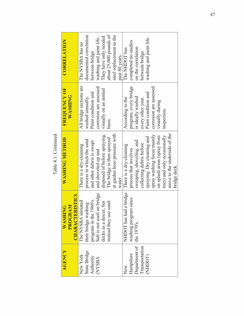
47
Tab
le 4
.1:
Co
nti
nu
ed
AG
EN
CY
W
AS
HIN
G
PR
OG
RA
M
CH
AR
AC
TE
RIS
TIC
S
WA
SH
ING
ME
TH
OD
F
RE
QU
EN
CY
OF
WA
SH
ING
CO
RR
EL
AT
ION
New
Yo
rk
Sta
te B
rid
ge
Au
tho
rity
(NY
SB
A
Th
e N
YS
BA
in
itia
ted
thei
r b
rid
ge
was
hin
g
pro
gra
m i
n t
he
19
60
's.
Sal
t is
no
t u
sed o
n b
rid
ge
dec
ks
as a
dei
cer,
bu
t
inst
ead
th
ey u
se s
and
.
Th
ere
is a
dry
-cle
anin
g
pro
cess
in
wh
ich
th
e sa
nd
and
oth
er d
ebri
s is
sw
ept
and
sh
ov
eled
up
and
dis
po
sed
of
bef
ore
sp
rayin
g.
Th
e b
rid
ge
is t
hen
sp
rayed
at g
ard
en h
ose
pre
ssu
re w
ith
wat
er.
All
bri
dge
sect
ion
s ar
e
was
hed
ann
ual
ly.
Pai
nt
con
dit
ion
and
corr
osi
on
are
ass
esse
d
vis
ual
ly o
n a
n a
nn
ual
bas
is.
Th
e N
YS
BA
has
no
do
cum
ente
d c
orr
elat
ion
bet
wee
n b
rid
ge
was
hin
g a
nd
pai
nt
life
.
Th
ey h
ave
on
ly n
eed
ed
abo
ut
25
,00
0 p
ou
nd
s o
f
stee
l re
pla
cem
ent
in t
he
pas
t 8
0 y
ears
.
New
Ham
psh
ire
Dep
artm
ent
of
Tra
nsp
ort
atio
n
(NH
DO
T)
NH
DO
T h
as h
ad a
bri
dg
e
was
hin
g p
rogra
m s
ince
the
19
70
's.
Th
ere
is a
dry
-cle
anin
g
pro
cess
th
at i
nv
olv
es
swee
pin
g,
sho
vel
ing,
and
coll
ecti
ng d
ebri
s b
efo
re
spra
yin
g.
Dry
cle
anin
g a
nd
spra
y w
ash
ing f
ocu
s m
ain
ly
on
sp
lash
are
as (
spra
y f
rom
tire
s) a
nd
on
ly o
ccas
ion
ally
mo
ve
to t
he
un
der
sid
e o
f th
e
bri
dge
dec
k.
Acc
ord
ing t
o t
he
pro
gra
m,
ever
y b
rid
ge
is i
dea
lly w
ash
ed
ever
y o
ther
yea
r.
Pai
nt
con
dit
ion
and
corr
osi
on
are
ass
esse
d
vis
ual
ly d
uri
ng
insp
ecti
on
.
Th
e N
HD
OT
has
com
ple
ted n
o s
tudie
s
on
th
e co
rrel
atio
n
bet
wee
n b
rid
ge
was
hin
g a
nd
pai
nt
life
.
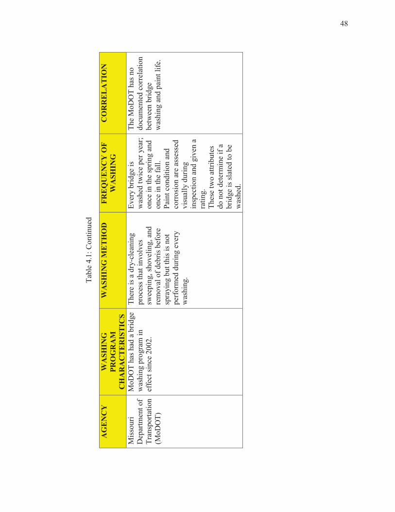
48
Tab
le 4
.1:
Co
nti
nu
ed
AG
EN
CY
W
AS
HIN
G
PR
OG
RA
M
CH
AR
AC
TE
RIS
TIC
S
WA
SH
ING
ME
TH
OD
F
RE
QU
EN
CY
OF
WA
SH
ING
CO
RR
EL
AT
ION
Mis
sou
ri
Dep
artm
ent
of
Tra
nsp
ort
atio
n
(Mo
DO
T)
Mo
DO
T h
as h
ad a
bri
dge
was
hin
g p
rogra
m i
n
effe
ct s
ince
20
02
.
Th
ere
is a
dry
-cle
anin
g
pro
cess
th
at i
nv
olv
es
swee
pin
g,
sho
vel
ing,
and
rem
ov
al o
f d
ebri
s b
efo
re
spra
yin
g b
ut
this
is
no
t
per
form
ed d
uri
ng e
ver
y
was
hin
g.
Ev
ery b
rid
ge
is
was
hed
tw
ice
per
yea
r;
on
ce i
n t
he
spri
ng a
nd
on
ce i
n t
he
fall
.
Pai
nt
con
dit
ion
and
corr
osi
on
are
ass
esse
d
vis
ual
ly d
uri
ng
insp
ecti
on
and
giv
en a
rati
ng.
Th
ese
two
att
rib
ute
s
do
no
t d
eter
min
e if
a
bri
dge
is s
late
d t
o b
e
was
hed
.
Th
e M
oD
OT
has
no
do
cum
ente
d c
orr
elat
ion
bet
wee
n b
rid
ge
was
hin
g a
nd
pai
nt
life
.
49
From Table 4.1 is observed that some DOT agencies perform a regular bridge washing
program. Some State DOTs started their washing program early in the 1960’s and 1970’s,
while other State DOTs started more recently in the 2000’s. Most of the washing
programs include a previous dry-cleaning, collecting debris and solid waste before spray
washing the steel girders with pressured water. The most common frequency for bridge
washing is every other year, while only New York State Bridge Authority performs the
activity every year. The most relevant observation from Table 4.1 is that none of the
referred State DOTs have studied or documented a correlation between bridge washing
activity and paint life performance. This is the fact that justify a research to find some
type of correlation between those two parameters.
4.2.2 Bridge Superstructure Washing Benefits
Bridge superstructure washing is accepted by several DOT agencies as an effective
maintenance activity that can reduce the rate of corrosion on steel members. Extending
the steel girders service life has a direct influence on bridge structure preservation and
integrity. Appleman et al. (1995), Hara et al. (2005), and Crampton et al. (2013)
concluded that superstructure water washing is a useful activity to suppress corrosion due
to deicing salt products and other compounds. Additionally, bridge superstructure
washing has positive effects on bridge inspection quality, providing a safe and clean steel
surface to be inspected and rated (RIDOT, 2002; Crampton et al. 2013). Figure 4.3 shows
the interior of a steel truss member with accumulated debris and the same section with
the corroded surface found after the debris was eliminated.

50
Figure 4.3: Interior of lower chord from truss. Before (left) and after (right) cleaning and
washing (Berman et al., 2013)
4.3 Spot Painting
To protect steel highway bridge girders from corrosion attack, the application of a coating
system when the girders are built is the most common practice. The coating systems used
20 – 30 years ago were lead-based paint systems without surface treatment. Due to
environmental concerns, the coating systems composition changed in the last couple of
decades to include the use of more environmentally friendly compounds. The
environmental and safety requirements for removing lead-based paints and other
chemical pollutants from the surfaces of steel bridge members have increased
exponentially, along with the cost of these abatement activities. Because of the ostensible
cost, many DOT agencies have decided not to repaint steel highway bridges. Due to
expected coat damages on structural steel members, a paint repair is frequently required.
As an alternative to a total bridge re-coating, spot painting is considered an efficient
solution when only few, and very small, portions of the coating are damaged. Spot
painting is expected as an economical alternative when no more than 1% of the total
surface area is damaged or it is rated on grade 7 or less in the scale presented in the
standard ASTM D610 “Standard Practice for Evaluating Degree of Rusting on Painted
Steel Surface” (ASTM, 2012).
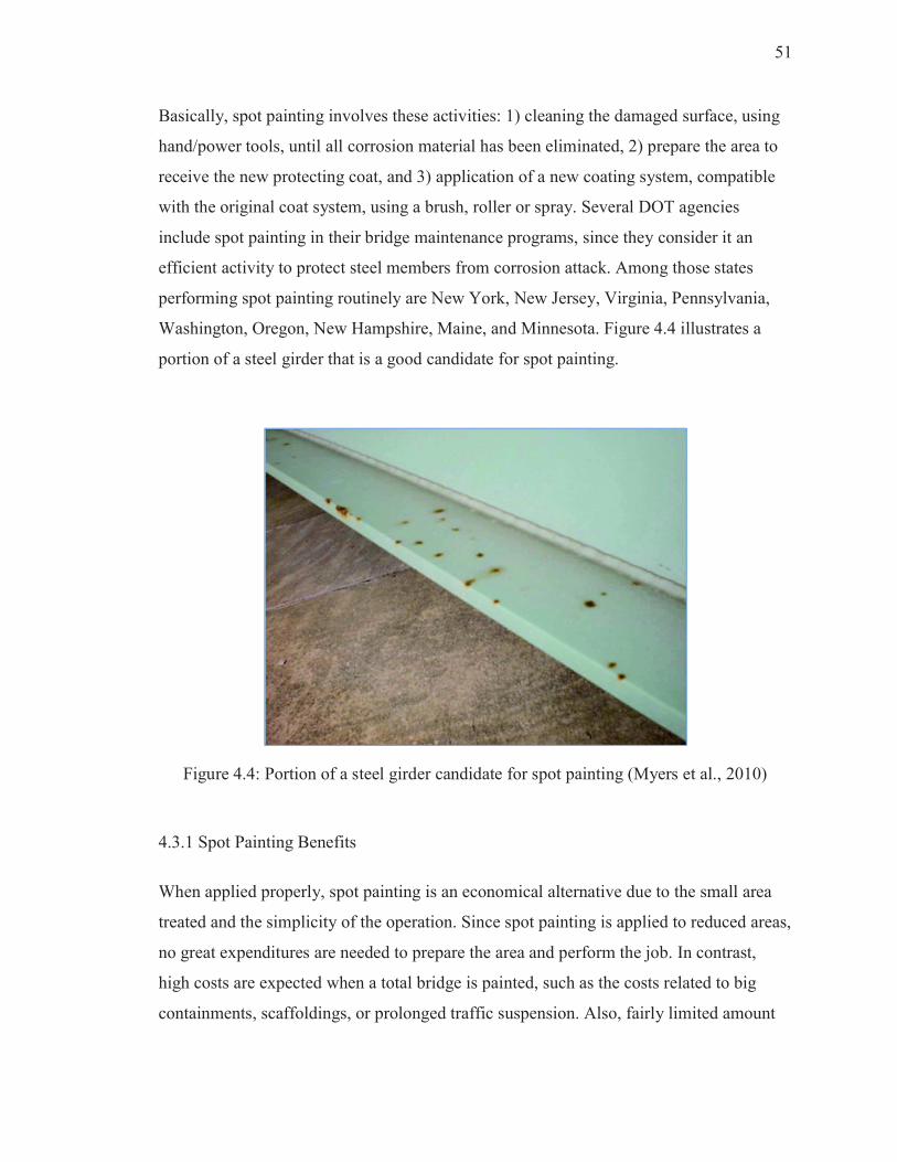
51
Basically, spot painting involves these activities: 1) cleaning the damaged surface, using
hand/power tools, until all corrosion material has been eliminated, 2) prepare the area to
receive the new protecting coat, and 3) application of a new coating system, compatible
with the original coat system, using a brush, roller or spray. Several DOT agencies
include spot painting in their bridge maintenance programs, since they consider it an
efficient activity to protect steel members from corrosion attack. Among those states
performing spot painting routinely are New York, New Jersey, Virginia, Pennsylvania,
Washington, Oregon, New Hampshire, Maine, and Minnesota. Figure 4.4 illustrates a
portion of a steel girder that is a good candidate for spot painting.
Figure 4.4: Portion of a steel girder candidate for spot painting (Myers et al., 2010)
4.3.1 Spot Painting Benefits
When applied properly, spot painting is an economical alternative due to the small area
treated and the simplicity of the operation. Since spot painting is applied to reduced areas,
no great expenditures are needed to prepare the area and perform the job. In contrast,
high costs are expected when a total bridge is painted, such as the costs related to big
containments, scaffoldings, or prolonged traffic suspension. Also, fairly limited amount
52
of debris and pollutants are expected to be eliminated. Due to the relatively small area to
be treated in spot painting work, little material is required, and it can be prepared at the
site without complicated procedures. The spot painting crew could move rapidly to treat
several spots in the same girder and the same bridge in a simple journey. Due to the basic
equipment required to perform spot painting, the traffic under the bridge is not
interrupted or it has to be partially interrupted for short periods of time only (Lanterman,
2009; Rea, 2014).
According to Lanterman (2009) and Rossow (2014), spot painting should be performed
as soon as possible to obtain maximum benefits from this activity. When not performed
at an early stage, the corrosion progress in the damaged area will be more significant and
the repair will require a more complex and expensive treatment.
4.3.2 Service Life of Spot Painting
The study from Chang (1999) indicated that several factors influence the service life of a
coating system, including: climate, coating age, traffic conditions, and maintenance
practices. Based on coating specifications, the most important requirement to achieve the
maximum service life from a coating system is the application process, including an
appropriate surface treatment prior to the coating application. Table 4.2 shows the
estimated service life of spot painting from several research studies, presented in the
study from Bowman and Moran (2015). It can be observed from Table 4.2 a wide
variation in the mean and range of expected values for the service life of spot painting,
according to those different studies. The large variation on the service life of spot
painting could be explained by the influence of the several factors that affect the coating
performance.

53
Table 4.2: Service life of spot painting (Bowman and Moran, 2015)
Researcher/DOTService Life (years)
Chang, 1999 15
Zayed et al., 2001 15
Chan, 2003 10 - 15
Yuan, 2005 10 - 15
Helsel et al., 2008 4 - 5
Petcherdchoo et al., 2008 10 - 15
MDOT, 2011 5
Yunovich et al., 2014 4
4.4 Summary
Although there is a lack of conclusive evidence, superstructure bridge washing is
considered for several DOT agencies as an efficient alternative to prolong the coating
system service life and reduce the corrosion attack on steel girders. There is an extensive
agreement between bridge inspectors, engineers, and maintenance crews, that regular
cleaning and washing of steel bridges is beneficial and will extend the structure service
life. Since this accepted agreement is based on opinions, beliefs and some performances,
more rigorous studies should be implemented on bridge washing. It is necessary to study
the benefits of bridge washing and the appropriate frequency of washing to obtain the
best benefits from the allocated resources when performing this activity.
Spot painting is a more studied activity, but predominantly from the automotive paint
sector. From the literature review it was found there is not a general agreement in the
expected service life for spot painting coats on steel girders. Therefore, more studies
applied on spot painting systems are required to support the benefits this maintenance
activity offers to extend the bridge service life.
54
ACCELERATED CORROSION TEST
5.1 Introduction
Steel bridges are exposed to very aggressive environments and must resist dead and live
loads throughout their entire service life, therefore, they require an adequate corrosion
protective system. “The most common corrosion protective systems have been the use of
either coating systems or weathering steel” (Bowman and Moran, 2015). Even the best
steel coating systems suffer damage due to manipulation during girder erection or
corrosion attack during their service life. Many State Department of Transportation
(DOTs) consider that regular bridge superstructure washing is an effective alternative to
reduce the damage due to atmospheric corrosion on steel substrate or coating layers
(Berman et al., 2013; Crampton et al., 2013). Also, spot painting has been identified as an
economical option to repair small and localized coating damage, avoiding the progress of
corrosion beyond the spot (Lanterman, 2009). The main objective of this study was to
analyze the performance of bridge superstructure washing and spot painting to determine
if these are effective maintenance activities to reduce the atmospheric corrosion process
on steel girder bridges.
The effect of superstructure washing was studied by performing a set of tests using steel
coupons under corrosion attack. The test program utilized two identical groups of
samples, one of them under a regular washing program and the second group without
washing.
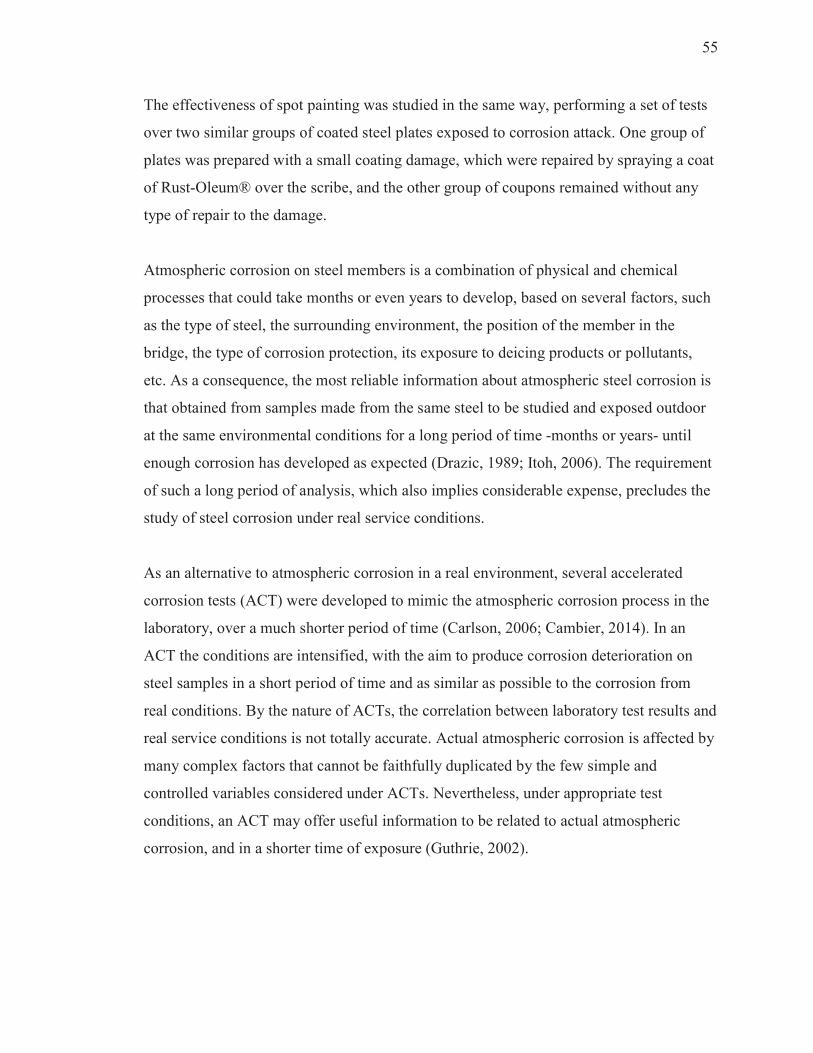
55
The effectiveness of spot painting was studied in the same way, performing a set of tests
over two similar groups of coated steel plates exposed to corrosion attack. One group of
plates was prepared with a small coating damage, which were repaired by spraying a coat
of Rust-Oleum® over the scribe, and the other group of coupons remained without any
type of repair to the damage.
Atmospheric corrosion on steel members is a combination of physical and chemical
processes that could take months or even years to develop, based on several factors, such
as the type of steel, the surrounding environment, the position of the member in the
bridge, the type of corrosion protection, its exposure to deicing products or pollutants,
etc. As a consequence, the most reliable information about atmospheric steel corrosion is
that obtained from samples made from the same steel to be studied and exposed outdoor
at the same environmental conditions for a long period of time -months or years- until
enough corrosion has developed as expected (Drazic, 1989; Itoh, 2006). The requirement
of such a long period of analysis, which also implies considerable expense, precludes the
study of steel corrosion under real service conditions.
As an alternative to atmospheric corrosion in a real environment, several accelerated
corrosion tests (ACT) were developed to mimic the atmospheric corrosion process in the
laboratory, over a much shorter period of time (Carlson, 2006; Cambier, 2014). In an
ACT the conditions are intensified, with the aim to produce corrosion deterioration on
steel samples in a short period of time and as similar as possible to the corrosion from
real conditions. By the nature of ACTs, the correlation between laboratory test results and
real service conditions is not totally accurate. Actual atmospheric corrosion is affected by
many complex factors that cannot be faithfully duplicated by the few simple and
controlled variables considered under ACTs. Nevertheless, under appropriate test
conditions, an ACT may offer useful information to be related to actual atmospheric
corrosion, and in a shorter time of exposure (Guthrie, 2002).
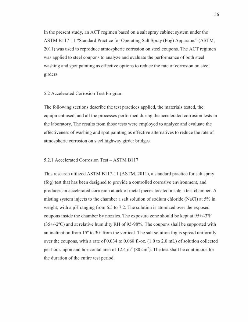
56
In the present study, an ACT regimen based on a salt spray cabinet system under the
ASTM B117-11 “Standard Practice for Operating Salt Spray (Fog) Apparatus” (ASTM,
2011) was used to reproduce atmospheric corrosion on steel coupons. The ACT regimen
was applied to steel coupons to analyze and evaluate the performance of both steel
washing and spot painting as effective options to reduce the rate of corrosion on steel
girders.
5.2 Accelerated Corrosion Test Program
The following sections describe the test practices applied, the materials tested, the
equipment used, and all the processes performed during the accelerated corrosion tests in
the laboratory. The results from those tests were employed to analyze and evaluate the
effectiveness of washing and spot painting as effective alternatives to reduce the rate of
atmospheric corrosion on steel highway girder bridges.
5.2.1 Accelerated Corrosion Test – ASTM B117
This research utilized ASTM B117-11 (ASTM, 2011), a standard practice for salt spray
(fog) test that has been designed to provide a controlled corrosive environment, and
produces an accelerated corrosion attack of metal pieces located inside a test chamber. A
misting system injects to the chamber a salt solution of sodium chloride (NaCl) at 5% in
weight, with a pH ranging from 6.5 to 7.2. The solution is atomized over the exposed
coupons inside the chamber by nozzles. The exposure zone should be kept at 95+/-3ºF
(35+/-2ºC) and at relative humidity RH of 95-98%. The coupons shall be supported with
an inclination from 15º to 30º from the vertical. The salt solution fog is spread uniformly
over the coupons, with a rate of 0.034 to 0.068 fl-oz. (1.0 to 2.0 mL) of solution collected
per hour, upon and horizontal area of 12.4 in2 (80 cm2). The test shall be continuous for
the duration of the entire test period.

57
5.2.2 Materials
The study considered two types of structural steel: carbon (plain) steel and weathering
steel. Two plates of carbon steel A709 Grade 50 with dimensions 4’ x 3’ x 0.5” and two
plates of weathering steel A709 Grade 50W with the same dimensions, were provided by
the Indiana Department of Transportation (INDOT) as part of their support for this
research. The mill test report for the two types of steel are presented in Appendix B,
detailing the mechanical properties and chemical composition for both steel types. For
each type of steel, one plate was coated and the other plate remained uncoated. The
coating system was applied by a certified INDOT contractor, in accordance to the
requirements established by INDOT standards (INDOT, 2012), consisting in a three-coat
system: an inorganic zinc primer, an epoxy intermediate coat, and a polyurethane finish
coat. The steel plates were cut in small coupons of 3” x 6” at the Central Machine Shop at
Purdue University.
The steel coupons were then protected with a casing made of a thick layer of 3M
Scotchkote Liquid Epoxy Coating 323, a two-part system designed to protect steel pieces
from harsh corrosion. The epoxy was applied to protect completely one face of the
coupon, all four edges, and the borders in the other face. Corrosion from cut edges
produces more rust than rolled surfaces, therefore all cut edges were protected to avoid
distortions due to this effect. The uncoated coupons presented a surface of 2 ½” x 5 ½”
and the coated coupons presented a surface of 2 ¼” x 5 ¼”, totally free to be exposed to
corrosion attack during tests. In this manner, the steel coupons offered only one face to be
exposed to corrosion while the rest of the plate was effectively protected. Figure 5.1
shows typical steel coupons before and after application of epoxy casing protection.
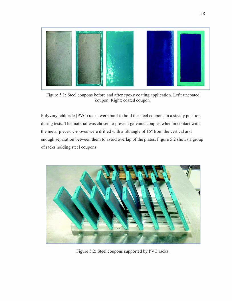
58
Figure 5.1: Steel coupons before and after epoxy coating application. Left: uncoated
coupon, Right: coated coupon.
Polyvinyl chloride (PVC) racks were built to hold the steel coupons in a steady position
during tests. The material was chosen to prevent galvanic couples when in contact with
the metal pieces. Grooves were drilled with a tilt angle of 15º from the vertical and
enough separation between them to avoid overlap of the plates. Figure 5.2 shows a group
of racks holding steel coupons.
Figure 5.2: Steel coupons supported by PVC racks.
59
Acrylic boxes (25” high, 20” wide, and 27” deep) were built to contain the steel coupons
inside the chamber under controlled temperature and relative humidity, as required by
ASTM B117. The boxes had space to contain 40 coupons supported by racks. Each box
had attachments to affix the misting system and keep 4 nozzles in a vertical position over
the coupons. The ceiling had a marked inclination, such that any drop of solution
accumulated in the upper inner surface would be directed to the sides. Figure 5.3 shows
an acrylic box with tubing connections to conduct the pumped salt solution to the
nozzles.
Figure 5.3: Front and lateral view of acrylic box
5.2.3 Equipment
5.2.3.1 Chamber
To perform the ACT following the ASTM B117 practice, a salt spray chamber was
adapted at the Pankow Materials Laboratory at Purdue University. A weather chamber
with automated controlled temperature from Darwin Chambers was assembled with a
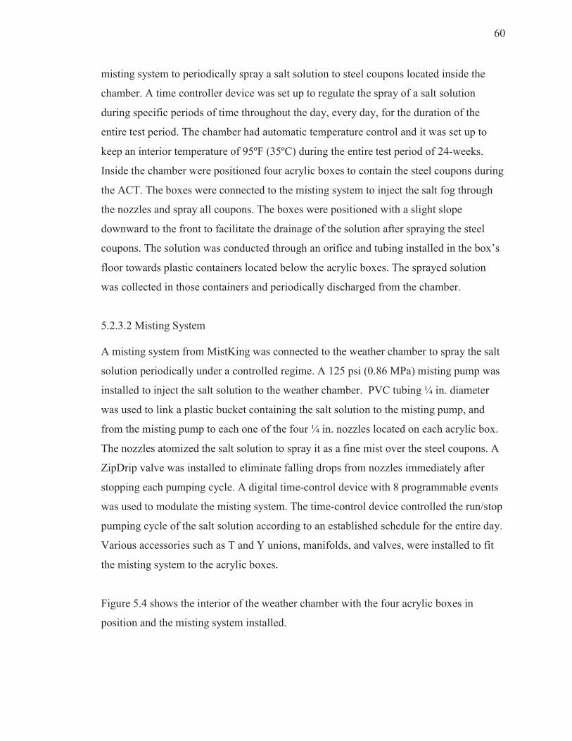
60
misting system to periodically spray a salt solution to steel coupons located inside the
chamber. A time controller device was set up to regulate the spray of a salt solution
during specific periods of time throughout the day, every day, for the duration of the
entire test period. The chamber had automatic temperature control and it was set up to
keep an interior temperature of 95ºF (35ºC) during the entire test period of 24-weeks.
Inside the chamber were positioned four acrylic boxes to contain the steel coupons during
the ACT. The boxes were connected to the misting system to inject the salt fog through
the nozzles and spray all coupons. The boxes were positioned with a slight slope
downward to the front to facilitate the drainage of the solution after spraying the steel
coupons. The solution was conducted through an orifice and tubing installed in the box’s
floor towards plastic containers located below the acrylic boxes. The sprayed solution
was collected in those containers and periodically discharged from the chamber.
5.2.3.2 Misting System
A misting system from MistKing was connected to the weather chamber to spray the salt
solution periodically under a controlled regime. A 125 psi (0.86 MPa) misting pump was
installed to inject the salt solution to the weather chamber. PVC tubing ¼ in. diameter
was used to link a plastic bucket containing the salt solution to the misting pump, and
from the misting pump to each one of the four ¼ in. nozzles located on each acrylic box.
The nozzles atomized the salt solution to spray it as a fine mist over the steel coupons. A
ZipDrip valve was installed to eliminate falling drops from nozzles immediately after
stopping each pumping cycle. A digital time-control device with 8 programmable events
was used to modulate the misting system. The time-control device controlled the run/stop
pumping cycle of the salt solution according to an established schedule for the entire day.
Various accessories such as T and Y unions, manifolds, and valves, were installed to fit
the misting system to the acrylic boxes.
Figure 5.4 shows the interior of the weather chamber with the four acrylic boxes in
position and the misting system installed.
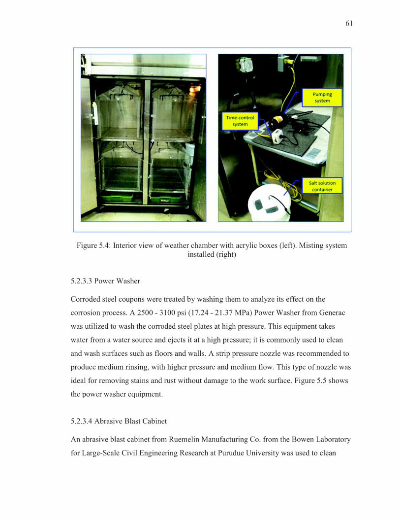
61
Figure 5.4: Interior view of weather chamber with acrylic boxes (left). Misting system
installed (right)
5.2.3.3 Power Washer
Corroded steel coupons were treated by washing them to analyze its effect on the
corrosion process. A 2500 - 3100 psi (17.24 - 21.37 MPa) Power Washer from Generac
was utilized to wash the corroded steel plates at high pressure. This equipment takes
water from a water source and ejects it at a high pressure; it is commonly used to clean
and wash surfaces such as floors and walls. A strip pressure nozzle was recommended to
produce medium rinsing, with higher pressure and medium flow. This type of nozzle was
ideal for removing stains and rust without damage to the work surface. Figure 5.5 shows
the power washer equipment.
5.2.3.4 Abrasive Blast Cabinet
An abrasive blast cabinet from Ruemelin Manufacturing Co. from the Bowen Laboratory
for Large-Scale Civil Engineering Research at Purudue University was used to clean
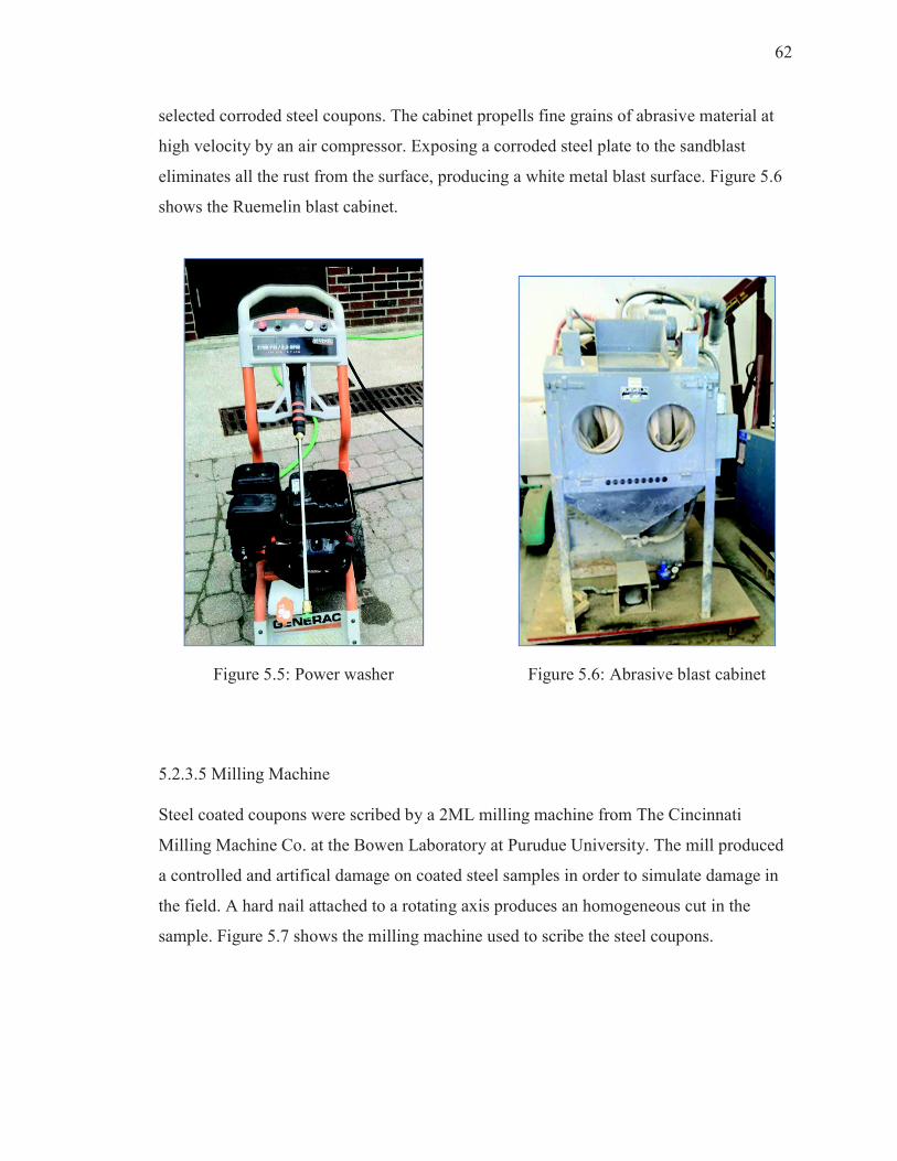
62
selected corroded steel coupons. The cabinet propells fine grains of abrasive material at
high velocity by an air compressor. Exposing a corroded steel plate to the sandblast
eliminates all the rust from the surface, producing a white metal blast surface. Figure 5.6
shows the Ruemelin blast cabinet.
Figure 5.5: Power washer
Figure 5.6: Abrasive blast cabinet
5.2.3.5 Milling Machine
Steel coated coupons were scribed by a 2ML milling machine from The Cincinnati
Milling Machine Co. at the Bowen Laboratory at Purudue University. The mill produced
a controlled and artifical damage on coated steel samples in order to simulate damage in
the field. A hard nail attached to a rotating axis produces an homogeneous cut in the
sample. Figure 5.7 shows the milling machine used to scribe the steel coupons.
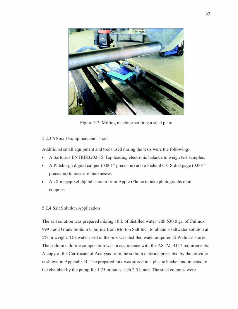
63
Figure 5.7: Milling machine scribing a steel plate
5.2.3.6 Small Equipment and Tools
Additional small equipment and tools used during the tests were the following:
· A Sartorius ENTRIS3202-1S Top loading electronic balance to weigh test samples.
· A Pittsburgh digital caliper (0.001” precision) and a Federal C81S dial gage (0.001”
precision) to measure thicknesses.
· An 8-megapixel digital camera from Apple iPhone to take photographs of all
coupons.
5.2.4 Salt Solution Application
The salt solution was prepared mixing 10 L of distilled water with 530.0 gr. of Culinox
999 Food Grade Sodium Clhoride from Morton Salt Inc., to obtain a saltwater solution at
5% in weight. The water used in the mix was distilled water adquired at Walmart stores.
The sodium chloride composition was in accordance with the ASTM-B117 requirements.
A copy of the Certificate of Analysis from the sodium chloride presented by the provider
is shown in Appendix B. The prepared mix was stored in a plastic bucket and injected to
the chamber by the pump for 1.25 minutes each 2.5 hours. The steel coupons were
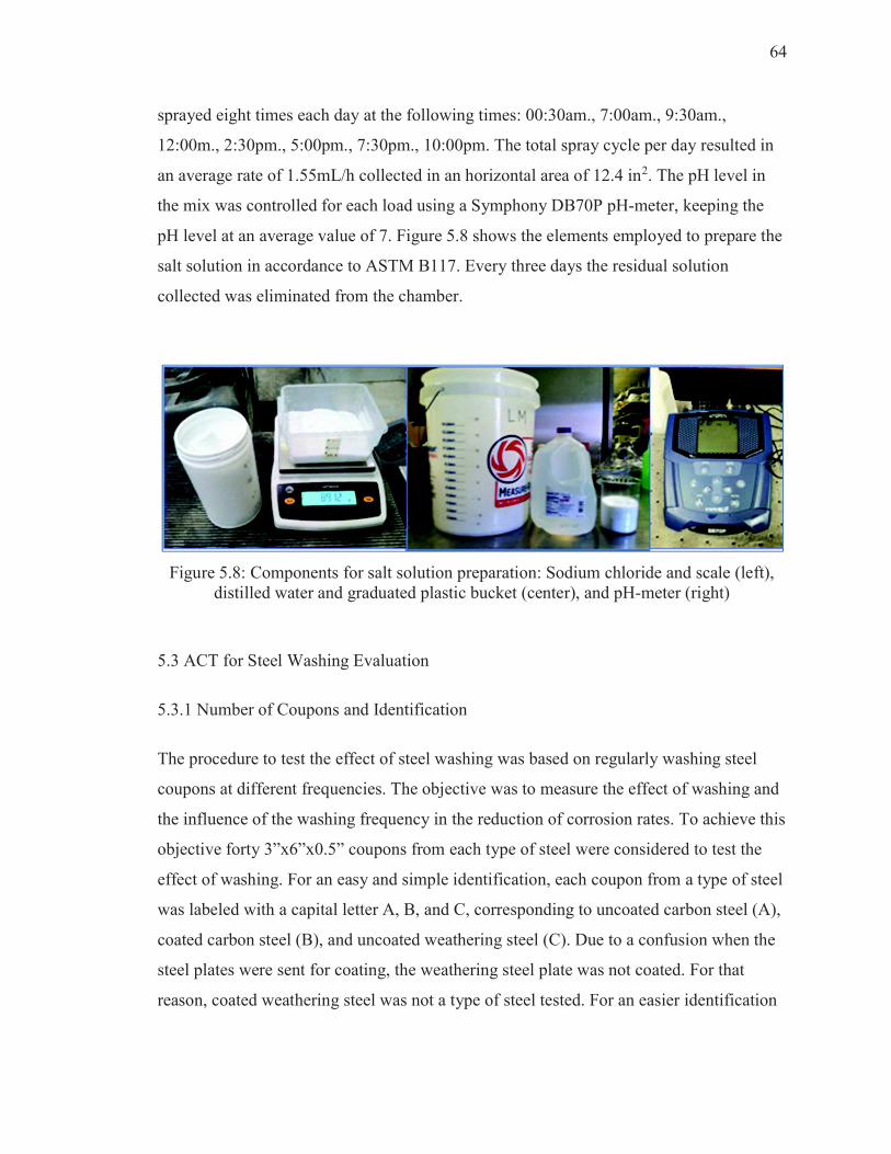
64
sprayed eight times each day at the following times: 00:30am., 7:00am., 9:30am.,
12:00m., 2:30pm., 5:00pm., 7:30pm., 10:00pm. The total spray cycle per day resulted in
an average rate of 1.55mL/h collected in an horizontal area of 12.4 in2. The pH level in
the mix was controlled for each load using a Symphony DB70P pH-meter, keeping the
pH level at an average value of 7. Figure 5.8 shows the elements employed to prepare the
salt solution in accordance to ASTM B117. Every three days the residual solution
collected was eliminated from the chamber.
Figure 5.8: Components for salt solution preparation: Sodium chloride and scale (left),
distilled water and graduated plastic bucket (center), and pH-meter (right)
5.3 ACT for Steel Washing Evaluation
5.3.1 Number of Coupons and Identification
The procedure to test the effect of steel washing was based on regularly washing steel
coupons at different frequencies. The objective was to measure the effect of washing and
the influence of the washing frequency in the reduction of corrosion rates. To achieve this
objective forty 3”x6”x0.5” coupons from each type of steel were considered to test the
effect of washing. For an easy and simple identification, each coupon from a type of steel
was labeled with a capital letter A, B, and C, corresponding to uncoated carbon steel (A),
coated carbon steel (B), and uncoated weathering steel (C). Due to a confusion when the
steel plates were sent for coating, the weathering steel plate was not coated. For that
reason, coated weathering steel was not a type of steel tested. For an easier identification
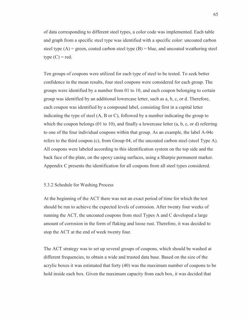
65
of data corresponding to different steel types, a color code was implemented. Each table
and graph from a specific steel type was identified with a specific color: uncoated carbon
steel type (A) = green, coated carbon steel type (B) = blue, and uncoated weathering steel
type (C) = red.
Ten groups of coupons were utilized for each type of steel to be tested. To seek better
confidence in the mean results, four steel coupons were considered for each group. The
groups were identified by a number from 01 to 10, and each coupon belonging to certain
group was identified by an additional lowercase letter, such as a, b, c, or d. Therefore,
each coupon was identified by a compound label, consisting first in a capital letter
indicating the type of steel (A, B or C), followed by a number indicating the group to
which the coupon belongs (01 to 10), and finally a lowercase letter (a, b, c, or d) referring
to one of the four individual coupons within that group. As an example, the label A-04c
refers to the third coupon (c), from Group 04, of the uncoated carbon steel (steel Type A).
All coupons were labeled according to this identification system on the top side and the
back face of the plate, on the epoxy casing surfaces, using a Sharpie permanent marker.
Appendix C presents the identification for all coupons from all steel types considered.
5.3.2 Schedule for Washing Process
At the beginning of the ACT there was not an exact period of time for which the test
should be run to achieve the expected levels of corrosion. After twenty four weeks of
running the ACT, the uncoated coupons from steel Types A and C developed a large
amount of corrosion in the form of flaking and loose rust. Therefore, it was decided to
stop the ACT at the end of week twenty four.
The ACT strategy was to set up several groups of coupons, which should be washed at
different frequencies, to obtain a wide and trusted data base. Based on the size of the
acrylic boxes it was estimated that forty (40) was the maximum number of coupons to be
hold inside each box. Given the maximum capacity from each box, it was decided that
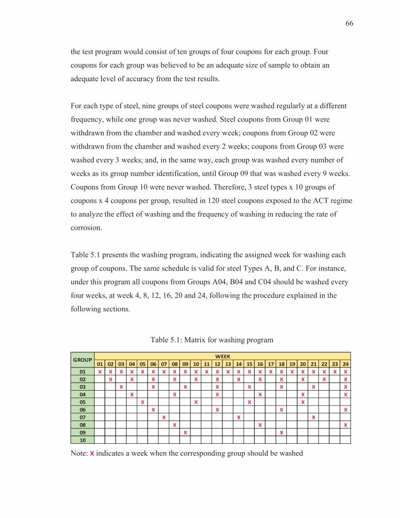
66
the test program would consist of ten groups of four coupons for each group. Four
coupons for each group was believed to be an adequate size of sample to obtain an
adequate level of accuracy from the test results.
For each type of steel, nine groups of steel coupons were washed regularly at a different
frequency, while one group was never washed. Steel coupons from Group 01 were
withdrawn from the chamber and washed every week; coupons from Group 02 were
withdrawn from the chamber and washed every 2 weeks; coupons from Group 03 were
washed every 3 weeks; and, in the same way, each group was washed every number of
weeks as its group number identification, until Group 09 that was washed every 9 weeks.
Coupons from Group 10 were never washed. Therefore, 3 steel types x 10 groups of
coupons x 4 coupons per group, resulted in 120 steel coupons exposed to the ACT regime
to analyze the effect of washing and the frequency of washing in reducing the rate of
corrosion.
Table 5.1 presents the washing program, indicating the assigned week for washing each
group of coupons. The same schedule is valid for steel Types A, B, and C. For instance,
under this program all coupons from Groups A04, B04 and C04 should be washed every
four weeks, at week 4, 8, 12, 16, 20 and 24, following the procedure explained in the
following sections.
Table 5.1: Matrix for washing program
01 02 03 04 05 06 07 08 09 10 11 12 13 14 15 16 17 18 19 20 21 22 23 24
01 X X X X X X X X X X X X X X X X X X X X X X X X
02 X X X X X X X X X X X X
03 X X X X X X X X
04 X X X X X X
05 X X X X
06 X X X X
07 X X X
08 X X X
09 X X
10
GROUPWEEK
Note: X indicates a week when the corresponding group should be washed

67
5.3.3 Initial Data Acquisition
The initial physical characteristics from each coupon were taken and registered before
beginning the ACT regimen. The weight, dimensions, thickness, and a photograph from
each steel coupon were registered before and after the application of the protective epoxy
casing used to expose only one coupon’s face to corrosion. The procedures for data
acquisition are presented in the next sections.
5.3.3.1 Weight
All coupons were weighed using the electronic balance, repeating the measurement three
times for a better precision. The initial weight of each coupon, after epoxy casing
application, are presented in Appendix D as data at week 0.
5.3.3.2 Dimensions
The top and bottom side dimensions for all coupons were measured using the digital
caliper. The initial side dimensions of all coupons, before epoxy casing application, are
presented in Appendix E.
5.3.3.3 Thickness
The thickness of each coupon was measured using two dial gages mounted in special
acrylic frames. One dial gage was attached to a frame fixed to measure the thicknesses at
points located at one fourth of the coupon width. The second dial gage was mounted to a
frame fixed to measure the thicknesses of points at the middle of the coupon width. A
plastic piece, the size of the steel coupon’s area was used as a template, with four
perforations at the one-fourth location of the coupon width and four perforations at the
middle of the coupon width. Using this template, the coupon thickness was measured at
twelve selected points, four at each one-fourth width and four at the middle of the coupon
width. Figure 5.9 shows the twelve points on a coupon where the thickness was
measured. The perforations in the plastic template were a little larger than the tip of the
spindle’s gage, enough to allow the spindle to fit the holes always in the same position.
68
The use of the plastic template helped to measure the thickness of a coupon in the same
twelve positions every time. The initial thickness of all the coupons, after epoxy casing
application, are presented in Appendix F.
Figure 5.9: Location of thickness measuring positions
5.3.3.4 Photographs
Each steel coupon was photographed using the digital camera from a smartphone. The
equipment was mounted in a special acrylic frame that helped to take photographs of the
coupons from the same distance and position each time. The initial photographs for each
coupon, before and after epoxy casing application, were registered and recorded in the
research database. Figure 5.10 shows the instruments utilized for coupon data acquisition,
such as weight, side dimensions, thickness, and photograph capture. In Appendix G are
presented all the photographs corresponding to coupon A01-a, for the twenty four weeks
the ACT lasted.

69
Figure 5.10: Coupon data acquisition. From left to right: weight, side dimensions,
thickness, photograph.
5.3.4 Procedure for the ACT Regime for Steel Washing Evaluation
The 120 steel coupons from Groups A, B, and C, were supported on the PVC racks and
placed inside the acrylic boxes. Each group of steel coupons was placed in one acrylic
box, forming four lines of racks, and containing ten coupons in each line. After the spray
process was initiated, the ACT continued every day for twenty four weeks, following the
indicated program of eight spray cycles per day. The salt solution bucket was loaded with
the 5% by weight of sodium chloride (NaCl) mix each three days to ensure a continuing
fog spray of the coupons inside the boxes. The spray system was controlled in a way that
never ran out of salt solution. Figure 5.11 shows the weather chamber with the acrylic
boxes containing the steel coupons during the ACT regime.

70
Figure 5.11: Weather chamber with steel coupons under ACT regime.
Every week, for the twenty four weeks (approximately 4000 hours) that the ACT lasted,
the groups of coupons were programmed for washing according to Table 5.1. The
programmed coupons were carefully removed from the chamber and submitted to a
protocol, which consisted of a series of treatments and data acquisition, as presented in
the next sections.
5.3.4.1 Removal from Chamber
Weekly every Thursday the coupons from the selected groups (see Table 5.1),
corresponding to the three steel Types A, B, and C, were withdrawn from the test
chamber to perform a series of treatments and physical observations. The remaining
coupons continued with the ACT process.
5.3.4.2 Power Washing
The selected steel coupons were placed on the floor, outside the laboratory for washing.
The steel coupons were kept an adequate distance between each other, with the corroded
face side up. The coupons were pressure-washed with the power washer machine,
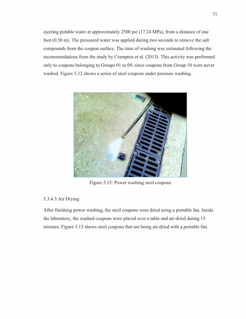
71
ejecting potable water at approximately 2500 psi (17.24 MPa), from a distance of one
foot (0.30 m). The pressured water was applied during two seconds to remove the salt
compounds from the coupon surface. The time of washing was estimated following the
recommendations from the study by Crampton et al. (2013). This activity was performed
only to coupons belonging to Groups 01 to 09, since coupons from Group 10 were never
washed. Figure 5.12 shows a series of steel coupons under pressure washing.
Figure 5.12: Power washing steel coupons
5.3.4.3 Air Drying
After finishing power washing, the steel coupons were dried using a portable fan. Inside
the laboratory, the washed coupons were placed over a table and air-dried during 15
minutes. Figure 5.13 shows steel coupons that are being air-dried with a portable fan.
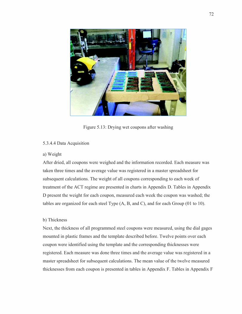
72
Figure 5.13: Drying wet coupons after washing
5.3.4.4 Data Acquisition
a) Weight
After dried, all coupons were weighed and the information recorded. Each measure was
taken three times and the average value was registered in a master spreadsheet for
subsequent calculations. The weight of all coupons corresponding to each week of
treatment of the ACT regime are presented in charts in Appendix D. Tables in Appendix
D present the weight for each coupon, measured each week the coupon was washed; the
tables are organized for each steel Type (A, B, and C), and for each Group (01 to 10).
b) Thickness
Next, the thickness of all programmed steel coupons were measured, using the dial gages
mounted in plastic frames and the template described before. Twelve points over each
coupon were identified using the template and the corresponding thicknesses were
registered. Each measure was done three times and the average value was registered in a
master spreadsheet for subsequent calculations. The mean value of the twelve measured
thicknesses from each coupon is presented in tables in Appendix F. Tables in Appendix F

73
present the thickness for each coupon, measured each week the coupon was washed, and
they are organized for each steel Type (A, B, and C), and for each Group (01 to 10).
c) Photograph Capture
All analyzed coupons were photographed to keep a visual record from physical changes
during the ACT. The photographs for all coupons tested during the ACT were registered
and recorded in the research database. In Appendix G are presented, as a manner of
example, all the photographs corresponding to coupon A01-a, for the twenty four weeks
the ACT lasted.
5.3.4.5 Return to Chamber
Finally, all the analyzed coupons were returned to the test chamber to continue the ACT
regime. The coupons were returned to the chamber in a different order than the original.
The position of coupons inside the box were changed every week to reduce some possible
influence of the location within the box on the rate of corrosion. Figure 5.14 presents a
flow chart with all the activities that are performed under the protocol of the ACT for
steel washing evaluation.
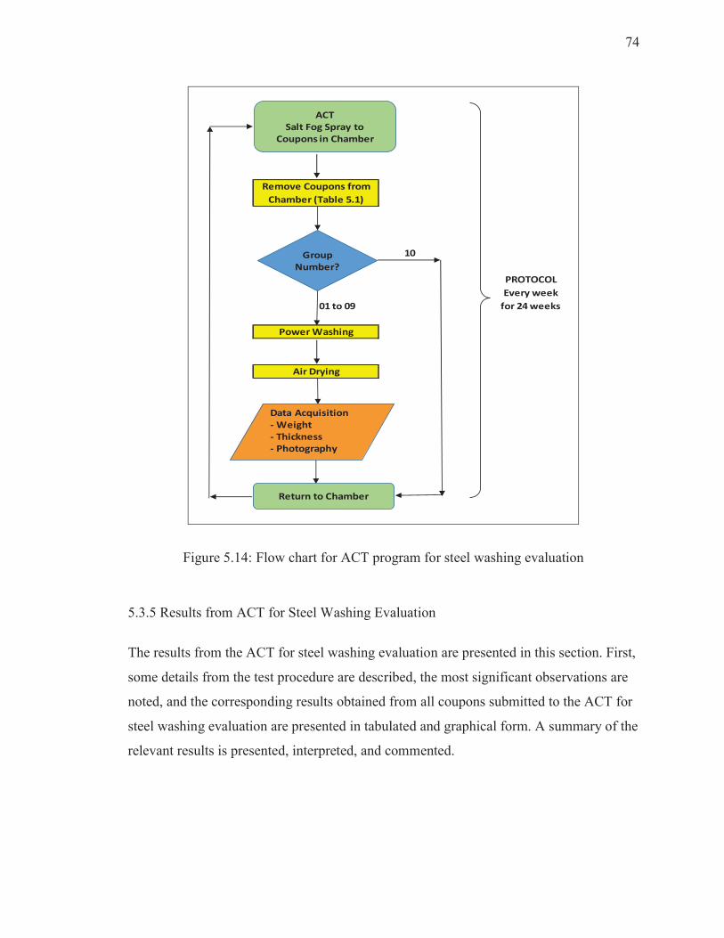
74
Figure 5.14: Flow chart for ACT program for steel washing evaluation
5.3.5 Results from ACT for Steel Washing Evaluation
The results from the ACT for steel washing evaluation are presented in this section. First,
some details from the test procedure are described, the most significant observations are
noted, and the corresponding results obtained from all coupons submitted to the ACT for
steel washing evaluation are presented in tabulated and graphical form. A summary of the
relevant results is presented, interpreted, and commented.
10
PROTOCOL
Every week
01 to 09 for 24 weeks
Air Drying
Remove Coupons from
Chamber (Table 5.1)
Power Washing
ACT
Salt Fog Spray to
Coupons in Chamber
Return to Chamber
Group
Number?
Data Acquisition
- Weight
- Thickness
- Photography
75
Few hours after the ACT started, the formation of the first spots of rust were observed on
the surfaces of both uncoated carbon and uncoated weathering steel coupons (steel Types
A and C respectively). The rust product was easily visualized and identified by its
characteristic orange to brown color in contrast to the steel gray color. The corrosion
degradation progressed gradually with time for the uncoated coupons, since the test
started and continued during the twenty four weeks the ACT lasted. During the salt spray
test the continuous fog caused the formation of drops in the corroded surface. With the
ACT progress, rough and flaky rust products grew on the surfaces of the uncoated
coupons (steel Types A and C). As could be observed from the photo-documented
evidence in Appendix G for coupon A01-a, the uncoated coupons developed significant
amount of rust products after the 24-weeks of exposure. The bottom edge of all uncoated
coupons showed a high grade of rust stain due to accumulation of corrosion products
between the coupons and the racks. A small formation of rust under the edges of the
epoxy casing, producing some cracks but without breaking the casing were observed in a
few uncoated coupons. The significant state of corrosion developed by the uncoated
coupons was the main reason to establish the end of the ACT at week 24.
Coated carbon steel coupons, labeled as steel Type B, showed no rust formation,
blistering, or any type of corrosion degradation in their exposed surface during the 24-
weeks the ACT lasted. Visual observation of all coated coupons showed undamaged
surfaces, even keeping almost the same gloss the coupons had at the beginning of the
ACT. The lack of corrosion defects on the coated surfaces after 4,000 hours of ACT
could be explained because the salt spray test did not include exposure to ultraviolet (UV)
light. UV light is considered a critical environmental factor affecting the paint gloss and
fading (Chong, 2007).
5.3.5.1 Weight Change
Data corresponding to the weight change from all steel coupons under the ACT are
presented in Appendix D. The recorded weight for each one of the 120 coupons
submitted to the ACT are presented in tabulated form. The tables present the weight for
76
each coupon measured each week the coupon was washed, classified by steel Types A, B,
and C, and by groups, from Group 01 to Group 10 respectively. Data for week 0 referred
to the initial weight, before the ACT started. Data were registered from week 0 to week
24, which is the last week of testing.
The weight change is also presented in graphical manner, showing the weight change
normalized by the coupon area exposed to corrosion. For each group of steel coupons a
graph is presented. Each graph represents the variation in time of the mean value of the
weight change corresponding to the four coupons for each group. The data were fitted
using functions from MS Excel to determine a representative curve for each group. For
steel Types A and C the data were best represented by a power function, which has a line
trace when it is plotted in log-log axes. For steel Type B, which shows values with little
variation, the data were best represented by a second order polynomial function, which is
showed in linear axes. In both cases the type of function was selected based on a
relatively high correlation parameter R2.
A review of the graphs in Appendix D, corresponding to steel Types A and C, shows a
similar pattern between groups of the same number (e.g. A04 with C04), with slightly
higher increment of weight on steel Type C coupons. For both steel Types A and C, the
pattern is an increment of coupon's weight in time. There is a direct relationship between
the increments of weight with the increment of corrosion rates, since the increment of
weight is generated by the production of rust due to underneath steel corrosion.
Observing the graphs for steel Type B coupons, the weight change values are almost
insignificant when compared to the values corresponding to steel Groups A or C. For that
reason, the graphs for steel Type B coupons are presented at a magnified scale for the
vertical axis. In the plots for steel Type B coupons, the common pattern is a slightly
increment of weight during the first few weeks of the test, followed by a continued
decrease of weight until the end of the test.
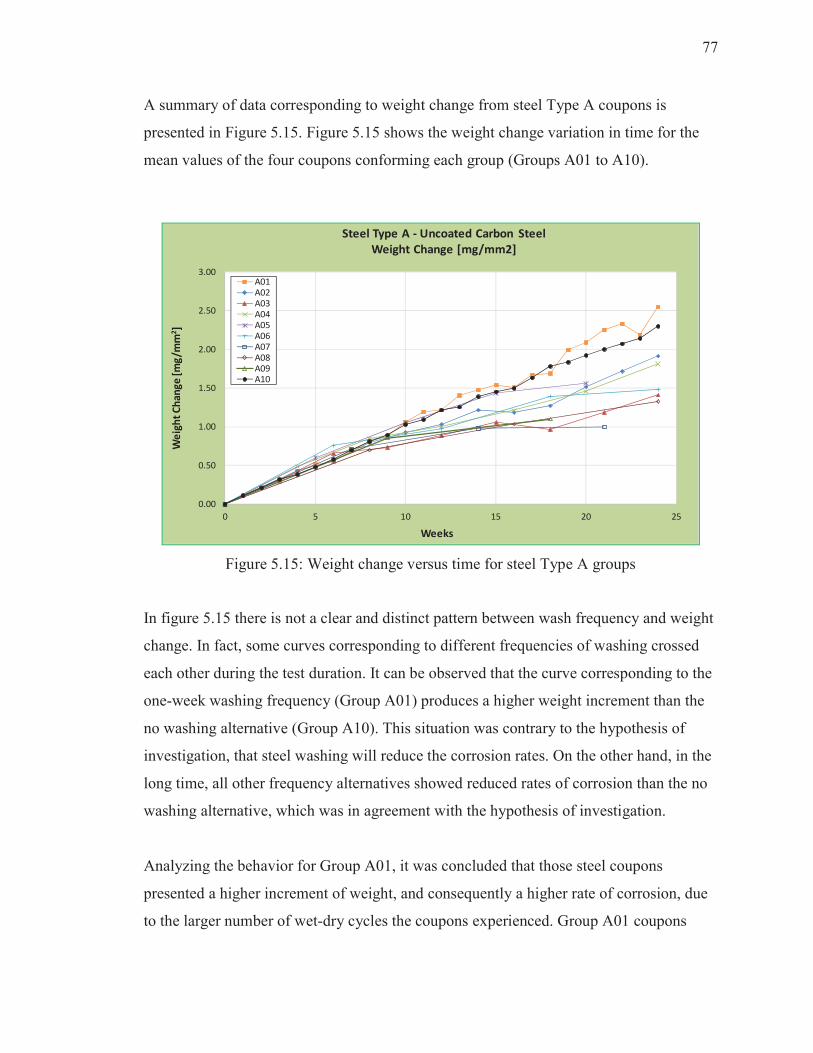
77
A summary of data corresponding to weight change from steel Type A coupons is
presented in Figure 5.15. Figure 5.15 shows the weight change variation in time for the
mean values of the four coupons conforming each group (Groups A01 to A10).
Figure 5.15: Weight change versus time for steel Type A groups
In figure 5.15 there is not a clear and distinct pattern between wash frequency and weight
change. In fact, some curves corresponding to different frequencies of washing crossed
each other during the test duration. It can be observed that the curve corresponding to the
one-week washing frequency (Group A01) produces a higher weight increment than the
no washing alternative (Group A10). This situation was contrary to the hypothesis of
investigation, that steel washing will reduce the corrosion rates. On the other hand, in the
long time, all other frequency alternatives showed reduced rates of corrosion than the no
washing alternative, which was in agreement with the hypothesis of investigation.
Analyzing the behavior for Group A01, it was concluded that those steel coupons
presented a higher increment of weight, and consequently a higher rate of corrosion, due
to the larger number of wet-dry cycles the coupons experienced. Group A01 coupons
0.00
0.50
1.00
1.50
2.00
2.50
3.00
0 5 10 15 20 25
We
igh
t C
han
ge
[mg
/mm
2]
Weeks
Steel Type A - Uncoated Carbon Steel
Weight Change [mg/mm2]
A01A02A03A04A05A06A07A08A09A10
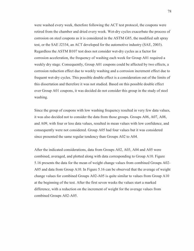
78
were washed every week, therefore following the ACT test protocol, the coupons were
retired from the chamber and dried every week. Wet-dry cycles exacerbate the process of
corrosion on steel coupons as it is considered in the ASTM G85, the modified salt spray
test, or the SAE J2334, an ACT developed for the automotive industry (SAE, 2003).
Regardless the ASTM B107 test does not consider wet-dry cycles as a factor for
corrosion acceleration, the frequency of washing each week for Group A01 required a
weekly dry stage. Consequently, Group A01 coupons could be affected by two effects, a
corrosion reduction effect due to weekly washing and a corrosion increment effect due to
frequent wet-dry cycles. This possible double effect is a consideration out of the limits of
this dissertation and therefore it was not studied. Based on this possible double effect
over Group A01 coupons, it was decided do not consider this group in the study of steel
washing.
Since the group of coupons with low washing frequency resulted in very few data values,
it was also decided not to consider the data from those groups. Groups A06, A07, A08,
and A09, with four or less data values, resulted in mean values with low confidence, and
consequently were not considered. Group A05 had four values but it was considered
since presented the same regular tendency than Groups A02 to A04.
After the indicated considerations, data from Groups A02, A03, A04 and A05 were
combined, averaged, and plotted along with data corresponding to Group A10. Figure
5.16 presents the data for the mean of weight change values from combined Groups A02-
A05 and data from Group A10. In Figure 5.16 can be observed that the average of weight
change values for combined Groups A02-A05 is quite similar to values from Group A10
at the beginning of the test. After the first seven weeks the values start a marked
difference, with a reduction on the increment of weight for the average values from
combined Groups A02-A05.

79
y = 0.11x0.97
R² = 0.99
y = 0.17x0.72
R² = 0.95
0.00
0.50
1.00
1.50
2.00
2.50
0 5 10 15 20 25
We
igh
t C
ha
ng
e [
mg
/mm
2]
Weeks
Steel Type A - Uncoated Carbon Steel
Weight Change [mg/mm2]
A10
A02-A05
Figure 5.16: Weight change versus time for mean values from Groups A02-A05 and
Group A10
Reducing the analyzed data to Groups A02 to A05 shows a more clear effect of steel
washing on reducing the rate of weight increment, and therefore, as explained previously,
a reduction of corrosion rates. In Figure 5.16 data corresponding to Group A10 present
higher rates of weight increment, and consequently, higher corrosion rates than data from
combined Groups A02-A05. Data points from the two plots in Figure 5.16 were fitted
using the least-squares function from MS Excel to determine a representative curve for
each group. Equations 5.1 and 5.2 show the power functions representing the weight
change for Groups A02-A05 and Group A10 respectively. In both cases the type of
function was selected based on a relatively high correlation parameter R2.
W1 � 0.17 ��.�� Equation 5.1
W2 � 0.11 ��. � Equation 5.2
where:
W1 = weight change for combined Groups A02-A05 [mg/mm2]
80
W2 = weight change for Group A10 [mg/mm2]
t = exposure time in ACT [weeks]
The same analysis and considerations applied to steel Type A coupons were applied to
the analysis for steel Type C coupons. Figure 5.17 shows the data corresponding to the
mean values of weight change variation in time for each group of coupons corresponding
to steel Type C (Groups C01 to C10). Figure 5.18 shows the data for the mean of weight
change values from combined Groups C02-C05 and data from Group C10. Again, it is
observed that there is less weight increment, and hence lower corrosion rates, from steel
washing alternatives (Groups C02-C05) versus the no washing alternative (Group C10).
Data points from the two plots were fitted using the least-squares function from MS
Excel to determine a representative curve for each group. Equations 5.3 and 5.4 show the
power functions representing the weight change for Groups C02-A05 and Group C10
respectively. In both cases the type of function was selected based on a relatively high
correlation parameter R2.
Figure 5.17: Weight change versus time for steel Type C groups
0.00
0.50
1.00
1.50
2.00
2.50
3.00
3.50
0 5 10 15 20 25
We
igh
t C
ha
ng
e [
mg
/mm
2]
Weeks
Steel Type C - Uncoated Weathering Steel
Weight Change [mg/mm2]
C01C02C03C04C05C06C07C08C09C10

81
y = 0.15x0.98
R² = 0.99
y = 0.20x0.83
R² = 0.98
0.00
0.50
1.00
1.50
2.00
2.50
3.00
3.50
4.00
0 5 10 15 20 25
We
igh
t C
ha
ng
e [
mg
/mm
2]
Weeks
Steel Type C - Uncoated Weathering Steel
Weight Change [mg/mm2]
C10
C02-C05
Figure 5.18: Weight change versus time for mean values from Groups C02-C05 and
Group C10
W3 � 0.20 ��.�� Equation 5.3
W4 � 0.15 ��. � Equation 5.4
where:
W3 = weight change for combined Groups C02-C05 [mg/mm2]
W4 = weight change for Group C10 [mg/mm2]
t = exposure time in ACT [weeks]
Data corresponding to weight change variation in time for the mean values of steel Type
B coupons are summarized in Figure 5.19. Plots from all Groups B01 to B10 do not show
a consistently pattern between wash frequency and weight change. From Figure 5.19 it is
observed a small tendency in all coupons to increase the weight at the beginning of the
test, and approximately after the week twelve to fifteen, the tendency is to reduce the
weight. It is important to emphasize the fact that weight changes for steel coupons from
steel Type B are very small (max. value of 0.10 mg/mm2) and irrelevant when compared
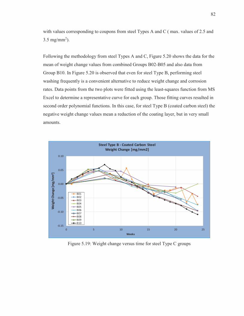
82
with values corresponding to coupons from steel Types A and C ( max. values of 2.5 and
3.5 mg/mm2).
Following the methodology from steel Types A and C, Figure 5.20 shows the data for the
mean of weight change values from combined Groups B02-B05 and also data from
Group B10. In Figure 5.20 is observed that even for steel Type B, performing steel
washing frequently is a convenient alternative to reduce weight change and corrosion
rates. Data points from the two plots were fitted using the least-squares function from MS
Excel to determine a representative curve for each group. Those fitting curves resulted in
second order polynomial functions. In this case, for steel Type B (coated carbon steel) the
negative weight change values mean a reduction of the coating layer, but in very small
amounts.
Figure 5.19: Weight change versus time for steel Type C groups
-0.15
-0.10
-0.05
0.00
0.05
0.10
0 5 10 15 20 25
We
igh
t C
ha
ng
e [m
g/m
m2]
Weeks
Steel Type B - Coated Carbon Steel
Weight Change [mg/mm2]
B01B02B03B04B05B06B07B08B09B10
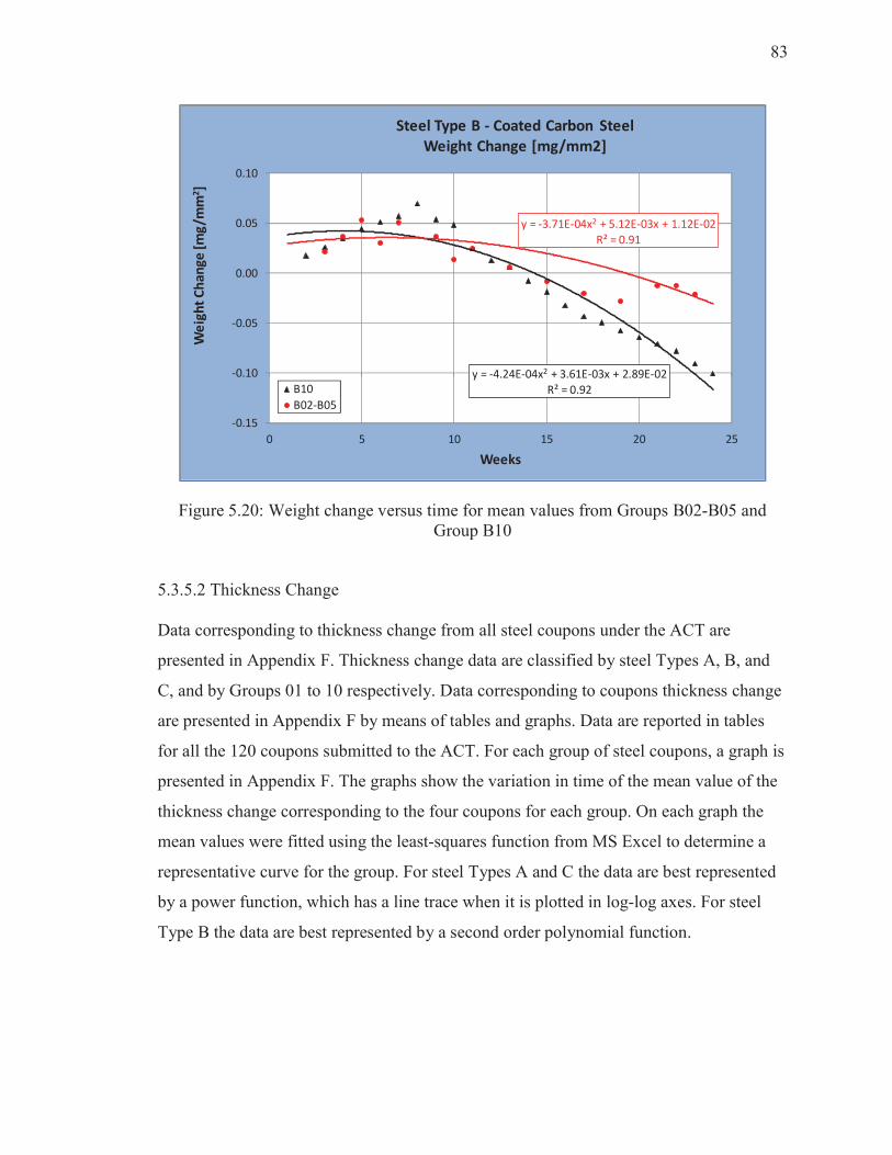
83
y = -4.24E-04x2 + 3.61E-03x + 2.89E-02
R² = 0.92
y = -3.71E-04x2 + 5.12E-03x + 1.12E-02
R² = 0.91
-0.15
-0.10
-0.05
0.00
0.05
0.10
0 5 10 15 20 25
We
igh
t C
ha
ng
e [
mg
/mm
2]
Weeks
Steel Type B - Coated Carbon Steel
Weight Change [mg/mm2]
B10
B02-B05
Figure 5.20: Weight change versus time for mean values from Groups B02-B05 and
Group B10
5.3.5.2 Thickness Change
Data corresponding to thickness change from all steel coupons under the ACT are
presented in Appendix F. Thickness change data are classified by steel Types A, B, and
C, and by Groups 01 to 10 respectively. Data corresponding to coupons thickness change
are presented in Appendix F by means of tables and graphs. Data are reported in tables
for all the 120 coupons submitted to the ACT. For each group of steel coupons, a graph is
presented in Appendix F. The graphs show the variation in time of the mean value of the
thickness change corresponding to the four coupons for each group. On each graph the
mean values were fitted using the least-squares function from MS Excel to determine a
representative curve for the group. For steel Types A and C the data are best represented
by a power function, which has a line trace when it is plotted in log-log axes. For steel
Type B the data are best represented by a second order polynomial function.
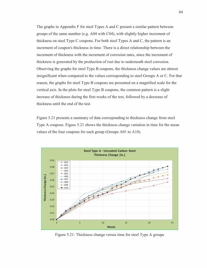
84
The graphs in Appendix F for steel Types A and C present a similar pattern between
groups of the same number (e.g. A04 with C04), with slightly higher increment of
thickness on steel Type C coupons. For both steel Types A and C, the pattern is an
increment of coupon's thickness in time. There is a direct relationship between the
increment of thickness with the increment of corrosion rates, since the increment of
thickness is generated by the production of rust due to underneath steel corrosion.
Observing the graphs for steel Type B coupons, the thickness change values are almost
insignificant when compared to the values corresponding to steel Groups A or C. For that
reason, the graphs for steel Type B coupons are presented on a magnified scale for the
vertical axis. In the plots for steel Type B coupons, the common pattern is a slight
increase of thickness during the first weeks of the test, followed by a decrease of
thickness until the end of the test.
Figure 5.21 presents a summary of data corresponding to thickness change from steel
Type A coupons. Figure 5.21 shows the thickness change variation in time for the mean
values of the four coupons for each group (Groups A01 to A10).
Figure 5.21: Thickness change versus time for steel Type A groups
0.00
0.01
0.02
0.03
0.04
0.05
0.06
0.07
0.08
0.09
0 5 10 15 20 25
Th
ick
ne
ss C
ha
ng
e [
in.]
Weeks
Steel Type A - Uncoated Carbon Steel
Thickness Change [in.]
A01A02A03A04A05A06A07A08A09A10
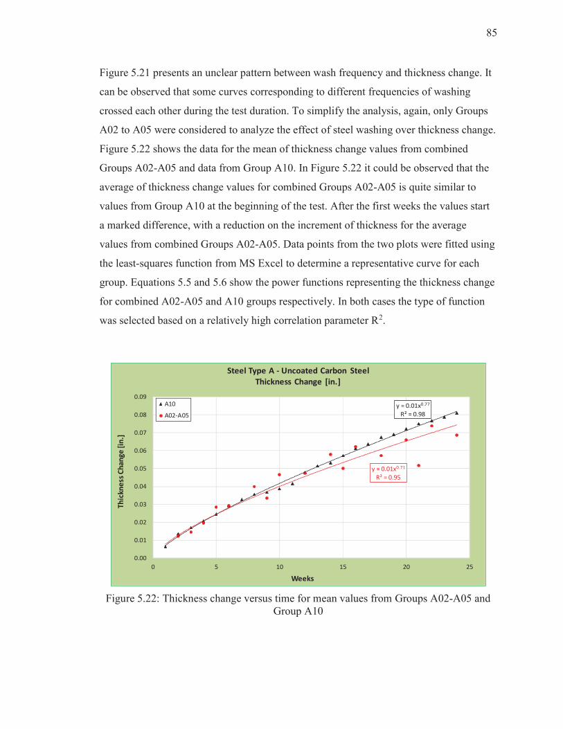
85
Figure 5.21 presents an unclear pattern between wash frequency and thickness change. It
can be observed that some curves corresponding to different frequencies of washing
crossed each other during the test duration. To simplify the analysis, again, only Groups
A02 to A05 were considered to analyze the effect of steel washing over thickness change.
Figure 5.22 shows the data for the mean of thickness change values from combined
Groups A02-A05 and data from Group A10. In Figure 5.22 it could be observed that the
average of thickness change values for combined Groups A02-A05 is quite similar to
values from Group A10 at the beginning of the test. After the first weeks the values start
a marked difference, with a reduction on the increment of thickness for the average
values from combined Groups A02-A05. Data points from the two plots were fitted using
the least-squares function from MS Excel to determine a representative curve for each
group. Equations 5.5 and 5.6 show the power functions representing the thickness change
for combined A02-A05 and A10 groups respectively. In both cases the type of function
was selected based on a relatively high correlation parameter R2.
y = 0.01x0.77
R² = 0.98
y = 0.01x0.71
R² = 0.95
0.00
0.01
0.02
0.03
0.04
0.05
0.06
0.07
0.08
0.09
0 5 10 15 20 25
Th
ickn
ess
Ch
an
ge
[in
.]
Weeks
Steel Type A - Uncoated Carbon Steel
Thickness Change [in.]
A10
A02-A05
Figure 5.22: Thickness change versus time for mean values from Groups A02-A05 and
Group A10
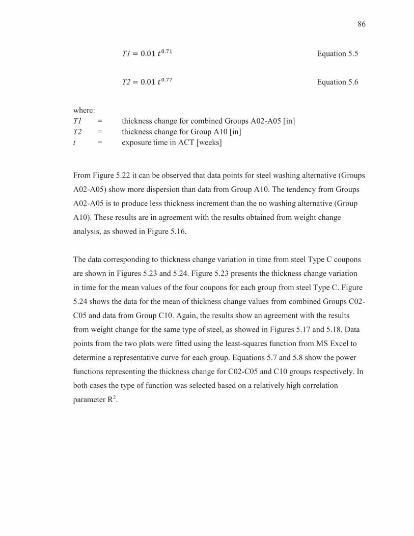
86
T1 � 0.01 ��.�� Equation 5.5
T2 � 0.01 ��.�� Equation 5.6
where:
T1 = thickness change for combined Groups A02-A05 [in]
T2 = thickness change for Group A10 [in]
t = exposure time in ACT [weeks]
From Figure 5.22 it can be observed that data points for steel washing alternative (Groups
A02-A05) show more dispersion than data from Group A10. The tendency from Groups
A02-A05 is to produce less thickness increment than the no washing alternative (Group
A10). These results are in agreement with the results obtained from weight change
analysis, as showed in Figure 5.16.
The data corresponding to thickness change variation in time from steel Type C coupons
are shown in Figures 5.23 and 5.24. Figure 5.23 presents the thickness change variation
in time for the mean values of the four coupons for each group from steel Type C. Figure
5.24 shows the data for the mean of thickness change values from combined Groups C02-
C05 and data from Group C10. Again, the results show an agreement with the results
from weight change for the same type of steel, as showed in Figures 5.17 and 5.18. Data
points from the two plots were fitted using the least-squares function from MS Excel to
determine a representative curve for each group. Equations 5.7 and 5.8 show the power
functions representing the thickness change for C02-C05 and C10 groups respectively. In
both cases the type of function was selected based on a relatively high correlation
parameter R2.
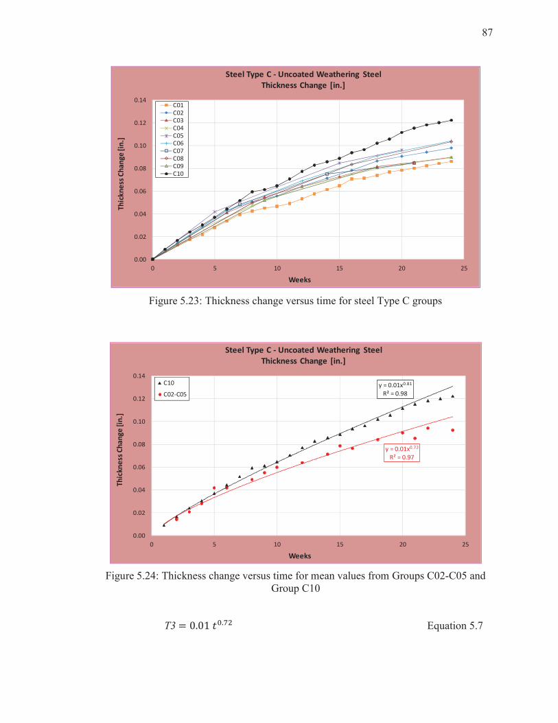
87
Figure 5.23: Thickness change versus time for steel Type C groups
y = 0.01x0.81
R² = 0.98
y = 0.01x0.72
R² = 0.97
0.00
0.02
0.04
0.06
0.08
0.10
0.12
0.14
0 5 10 15 20 25
Th
ickn
ess
Ch
an
ge
[in
.]
Weeks
Steel Type C - Uncoated Weathering Steel
Thickness Change [in.]
C10
C02-C05
Figure 5.24: Thickness change versus time for mean values from Groups C02-C05 and
Group C10
T3 � 0.01 ��.�� Equation 5.7
0.00
0.02
0.04
0.06
0.08
0.10
0.12
0.14
0 5 10 15 20 25
Th
ick
ne
ss C
ha
ng
e [
in.]
Weeks
Steel Type C - Uncoated Weathering Steel
Thickness Change [in.]
C01C02C03C04C05C06C07C08C09C10
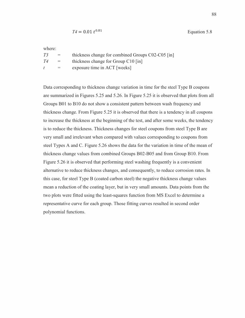
88
T4 � 0.01 ��.�� Equation 5.8
where:
T3 = thickness change for combined Groups C02-C05 [in]
T4 = thickness change for Group C10 [in]
t = exposure time in ACT [weeks]
Data corresponding to thickness change variation in time for the steel Type B coupons
are summarized in Figures 5.25 and 5.26. In Figure 5.25 it is observed that plots from all
Groups B01 to B10 do not show a consistent pattern between wash frequency and
thickness change. From Figure 5.25 it is observed that there is a tendency in all coupons
to increase the thickness at the beginning of the test, and after some weeks, the tendency
is to reduce the thickness. Thickness changes for steel coupons from steel Type B are
very small and irrelevant when compared with values corresponding to coupons from
steel Types A and C. Figure 5.26 shows the data for the variation in time of the mean of
thickness change values from combined Groups B02-B05 and from Group B10. From
Figure 5.26 it is observed that performing steel washing frequently is a convenient
alternative to reduce thickness changes, and consequently, to reduce corrosion rates. In
this case, for steel Type B (coated carbon steel) the negative thickness change values
mean a reduction of the coating layer, but in very small amounts. Data points from the
two plots were fitted using the least-squares function from MS Excel to determine a
representative curve for each group. Those fitting curves resulted in second order
polynomial functions.
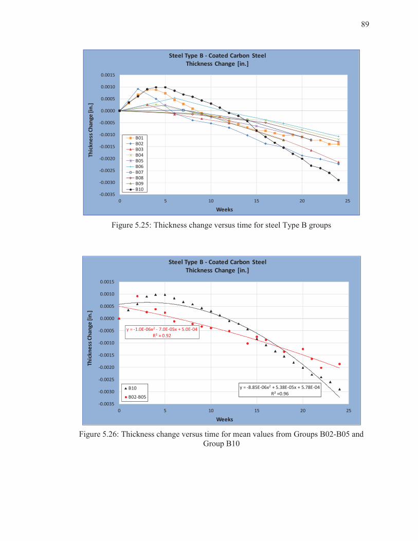
89
Figure 5.25: Thickness change versus time for steel Type B groups
y = -8.85E-06x2 + 5.38E-05x + 5.78E-04
R² =0.96
y = -1.0E-06x2 - 7.0E-05x + 5.0E-04
R² = 0.92
-0.0035
-0.0030
-0.0025
-0.0020
-0.0015
-0.0010
-0.0005
0.0000
0.0005
0.0010
0.0015
0 5 10 15 20 25
Th
ick
ne
ss C
ha
ng
e [
in.]
Weeks
Steel Type B - Coated Carbon Steel
Thickness Change [in.]
B10
B02-B05
Figure 5.26: Thickness change versus time for mean values from Groups B02-B05 and
Group B10
-0.0035
-0.0030
-0.0025
-0.0020
-0.0015
-0.0010
-0.0005
0.0000
0.0005
0.0010
0.0015
0 5 10 15 20 25
Th
ick
ne
ss C
ha
ng
e [
in.]
Weeks
Steel Type B - Coated Carbon Steel
Thickness Change [in.]
B01B02B03B04B05B06B07B08B09B10
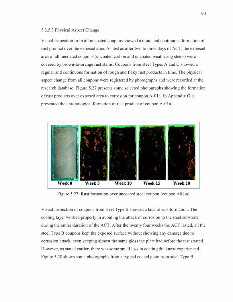
90
5.3.5.3 Physical Aspect Change
Visual inspection from all uncoated coupons showed a rapid and continuous formation of
rust product over the exposed area. As fast as after two to three days of ACT, the exposed
area of all uncoated coupons (uncoated carbon and uncoated weathering steels) were
covered by brown-to-orange rust stains. Coupons from steel Types A and C showed a
regular and continuous formation of rough and flaky rust products in time. The physical
aspect change from all coupons were registered by photographs and were recorded at the
research database. Figure 5.27 presents some selected photographs showing the formation
of rust products over exposed area to corrosion for coupon A-01a. In Appendix G is
presented the chronological formation of rust product of coupon A-01a.
Figure 5.27: Rust formation over uncoated steel coupon (coupon A01-a)
Visual inspection of coupons from steel Type B showed a lack of rust formation. The
coating layer worked properly in avoiding the attack of corrosion to the steel substrate
during the entire duration of the ACT. After the twenty four weeks the ACT lasted, all the
steel Type B coupons kept the exposed surface without showing any damage due to
corrosion attack, even keeping almost the same gloss the plate had before the test started.
However, as stated earlier, there was some small loss in coating thickness experienced.
Figure 5.28 shows some photographs from a typical coated plate from steel Type B.
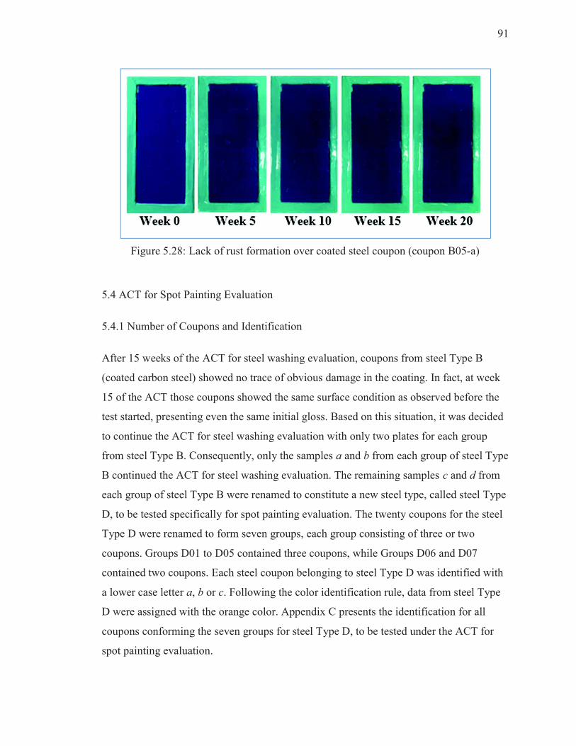
91
Figure 5.28: Lack of rust formation over coated steel coupon (coupon B05-a)
5.4 ACT for Spot Painting Evaluation
5.4.1 Number of Coupons and Identification
After 15 weeks of the ACT for steel washing evaluation, coupons from steel Type B
(coated carbon steel) showed no trace of obvious damage in the coating. In fact, at week
15 of the ACT those coupons showed the same surface condition as observed before the
test started, presenting even the same initial gloss. Based on this situation, it was decided
to continue the ACT for steel washing evaluation with only two plates for each group
from steel Type B. Consequently, only the samples a and b from each group of steel Type
B continued the ACT for steel washing evaluation. The remaining samples c and d from
each group of steel Type B were renamed to constitute a new steel type, called steel Type
D, to be tested specifically for spot painting evaluation. The twenty coupons for the steel
Type D were renamed to form seven groups, each group consisting of three or two
coupons. Groups D01 to D05 contained three coupons, while Groups D06 and D07
contained two coupons. Each steel coupon belonging to steel Type D was identified with
a lower case letter a, b or c. Following the color identification rule, data from steel Type
D were assigned with the orange color. Appendix C presents the identification for all
coupons conforming the seven groups for steel Type D, to be tested under the ACT for
spot painting evaluation.
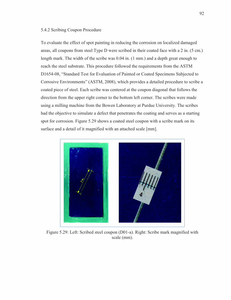
92
5.4.2 Scribing Coupon Procedure
To evaluate the effect of spot painting in reducing the corrosion on localized damaged
areas, all coupons from steel Type D were scribed in their coated face with a 2 in. (5 cm.)
length mark. The width of the scribe was 0.04 in. (1 mm.) and a depth great enough to
reach the steel substrate. This procedure followed the requirements from the ASTM
D1654-08, “Standard Test for Evaluation of Painted or Coated Specimens Subjected to
Corrosive Environments” (ASTM, 2008), which provides a detailed procedure to scribe a
coated piece of steel. Each scribe was centered at the coupon diagonal that follows the
direction from the upper right corner to the bottom left corner. The scribes were made
using a milling machine from the Bowen Laboratory at Purdue University. The scribes
had the objective to simulate a defect that penetrates the coating and serves as a starting
spot for corrosion. Figure 5.29 shows a coated steel coupon with a scribe mark on its
surface and a detail of it magnified with an attached scale [mm].
Figure 5.29: Left: Scribed steel coupon (D01-a). Right: Scribe mark magnified with
scale (mm).
93
5.4.3 Initial Data Acquisition
All coupons from steel Type D (Groups D01 to D07) were weighed and photographed
after scribing and the data were recorded to follow the progress of corrosion in the spot
damage during the ACT. Initial weights from all coupons from steel Type D are
presented in Appendix D. All coupons from steel Type D were photographed before the
test started and the photographs were recorded in the research database. Appendix H
presents the photographs for coupons D01-a and D02-b before exposure to the ACT.
5.4.4 Procedure for the ACT Regime for Spot Painting Evaluation
During six weeks the scribed coupons from steel Type D followed a similar ACT to that
used for the steel washing evaluation, as explained in section 5.3.3. The coupons from
Groups D01 to D04 were washed, dried, weighed, and photographed, with a frequency
according to Table 5.1. The coupons from Groups D05 to D07 were never washed, but
weighed and photographed, following the same schedule from Table 5.1. In this ACT
regime the coupon thickness change was not a variable to be measured. Each week, after
all data were acquired, the analyzed coupons were returned to the chamber, in a position
different from which they occupied previously. For each coupon from steel Type D, the
weights and photographs corresponding to each week of treatment of the ACT regime are
presented in Appendices D and H respectively. Figure 5.30 shows a flow chart for the
activities performed during the ACT regime for spot painting evaluation.
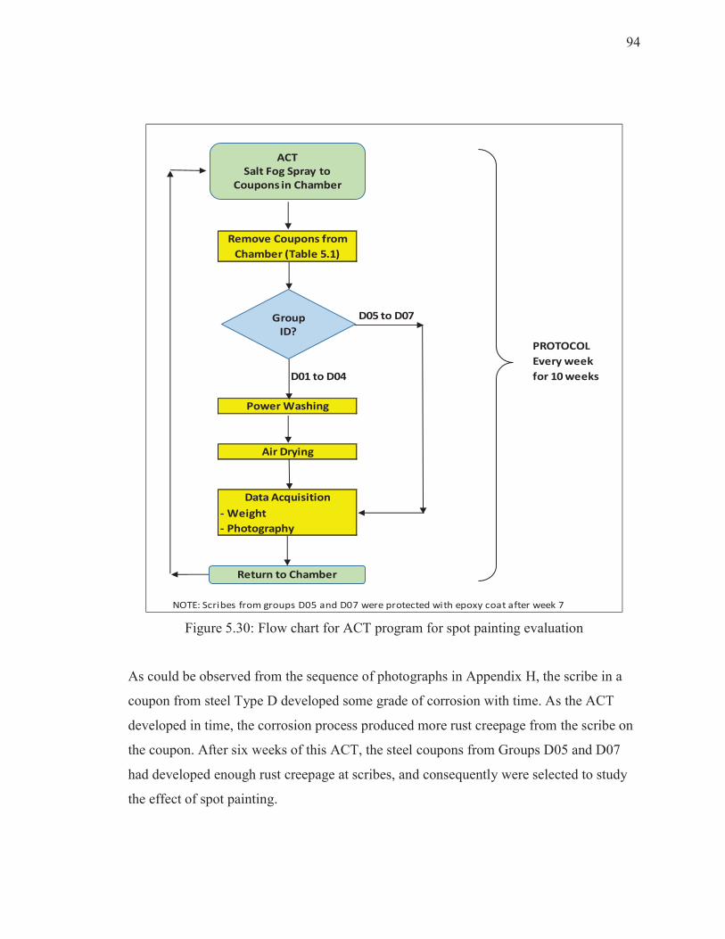
94
D05 to D07
PROTOCOL
Every week
D01 to D04 for 10 weeks
- Weight
- Photography
NOTE: Scribes from groups D05 and D07 were protected with epoxy coat after week 7
Air Drying
Data Acquisition
Remove Coupons from
Chamber (Table 5.1)
Power Washing
ACT
Salt Fog Spray to
Coupons in Chamber
Group
ID?
Return to Chamber
Figure 5.30: Flow chart for ACT program for spot painting evaluation
As could be observed from the sequence of photographs in Appendix H, the scribe in a
coupon from steel Type D developed some grade of corrosion with time. As the ACT
developed in time, the corrosion process produced more rust creepage from the scribe on
the coupon. After six weeks of this ACT, the steel coupons from Groups D05 and D07
had developed enough rust creepage at scribes, and consequently were selected to study
the effect of spot painting.
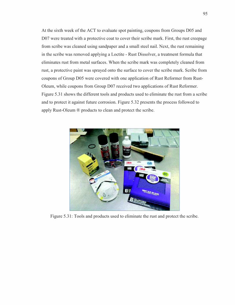
95
At the sixth week of the ACT to evaluate spot painting, coupons from Groups D05 and
D07 were treated with a protective coat to cover their scribe mark. First, the rust creepage
from scribe was cleaned using sandpaper and a small steel nail. Next, the rust remaining
in the scribe was removed applying a Loctite - Rust Dissolver, a treatment formula that
eliminates rust from metal surfaces. When the scribe mark was completely cleaned from
rust, a protective paint was sprayed onto the surface to cover the scribe mark. Scribe from
coupons of Group D05 were covered with one application of Rust Reformer from Rust-
Oleum, while coupons from Group D07 received two applications of Rust Reformer.
Figure 5.31 shows the different tools and products used to eliminate the rust from a scribe
and to protect it against future corrosion. Figure 5.32 presents the process followed to
apply Rust-Oleum ® products to clean and protect the scribe.
Figure 5.31: Tools and products used to eliminate the rust and protect the scribe.
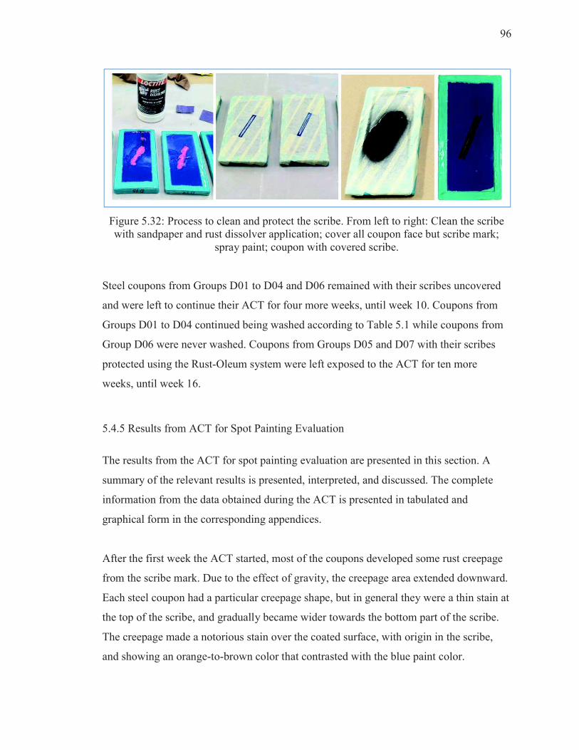
96
Figure 5.32: Process to clean and protect the scribe. From left to right: Clean the scribe
with sandpaper and rust dissolver application; cover all coupon face but scribe mark;
spray paint; coupon with covered scribe.
Steel coupons from Groups D01 to D04 and D06 remained with their scribes uncovered
and were left to continue their ACT for four more weeks, until week 10. Coupons from
Groups D01 to D04 continued being washed according to Table 5.1 while coupons from
Group D06 were never washed. Coupons from Groups D05 and D07 with their scribes
protected using the Rust-Oleum system were left exposed to the ACT for ten more
weeks, until week 16.
5.4.5 Results from ACT for Spot Painting Evaluation
The results from the ACT for spot painting evaluation are presented in this section. A
summary of the relevant results is presented, interpreted, and discussed. The complete
information from the data obtained during the ACT is presented in tabulated and
graphical form in the corresponding appendices.
After the first week the ACT started, most of the coupons developed some rust creepage
from the scribe mark. Due to the effect of gravity, the creepage area extended downward.
Each steel coupon had a particular creepage shape, but in general they were a thin stain at
the top of the scribe, and gradually became wider towards the bottom part of the scribe.
The creepage made a notorious stain over the coated surface, with origin in the scribe,
and showing an orange-to-brown color that contrasted with the blue paint color.
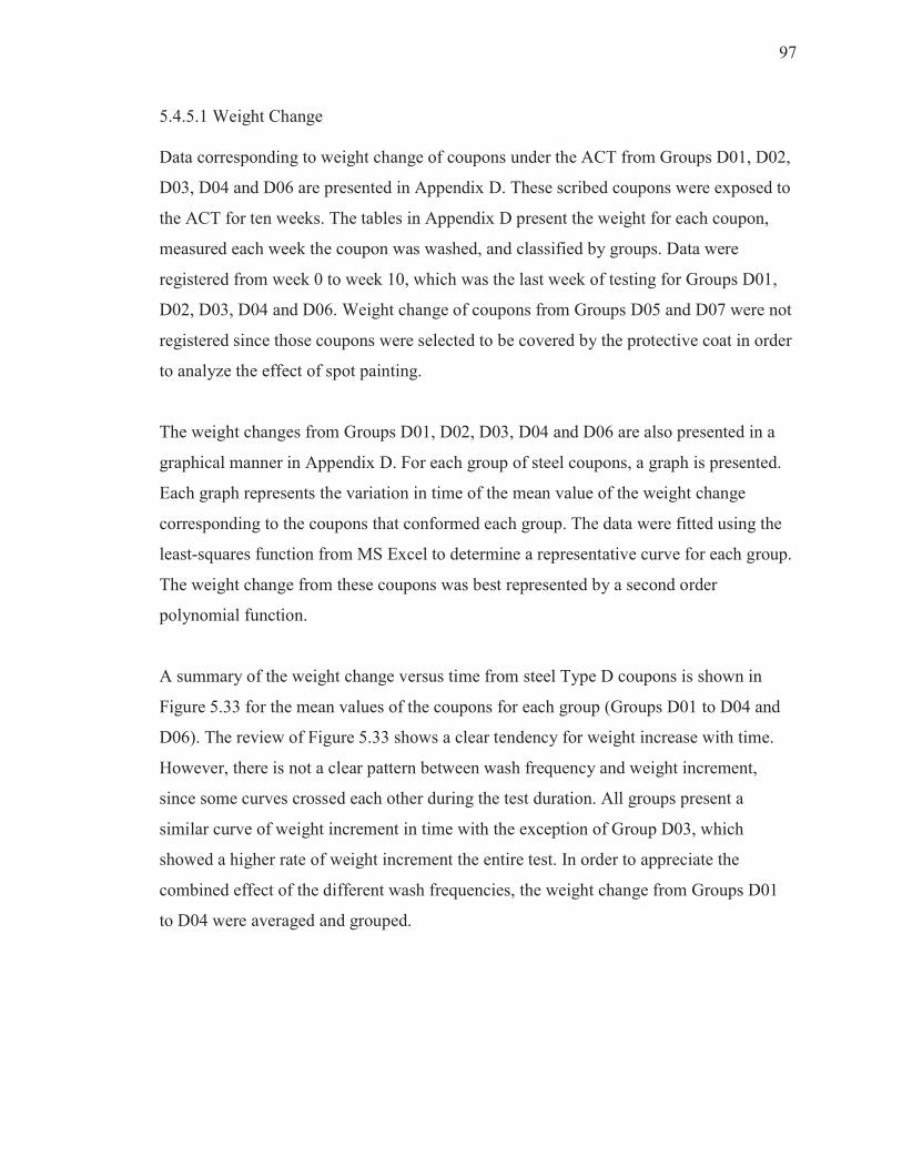
97
5.4.5.1 Weight Change
Data corresponding to weight change of coupons under the ACT from Groups D01, D02,
D03, D04 and D06 are presented in Appendix D. These scribed coupons were exposed to
the ACT for ten weeks. The tables in Appendix D present the weight for each coupon,
measured each week the coupon was washed, and classified by groups. Data were
registered from week 0 to week 10, which was the last week of testing for Groups D01,
D02, D03, D04 and D06. Weight change of coupons from Groups D05 and D07 were not
registered since those coupons were selected to be covered by the protective coat in order
to analyze the effect of spot painting.
The weight changes from Groups D01, D02, D03, D04 and D06 are also presented in a
graphical manner in Appendix D. For each group of steel coupons, a graph is presented.
Each graph represents the variation in time of the mean value of the weight change
corresponding to the coupons that conformed each group. The data were fitted using the
least-squares function from MS Excel to determine a representative curve for each group.
The weight change from these coupons was best represented by a second order
polynomial function.
A summary of the weight change versus time from steel Type D coupons is shown in
Figure 5.33 for the mean values of the coupons for each group (Groups D01 to D04 and
D06). The review of Figure 5.33 shows a clear tendency for weight increase with time.
However, there is not a clear pattern between wash frequency and weight increment,
since some curves crossed each other during the test duration. All groups present a
similar curve of weight increment in time with the exception of Group D03, which
showed a higher rate of weight increment the entire test. In order to appreciate the
combined effect of the different wash frequencies, the weight change from Groups D01
to D04 were averaged and grouped.
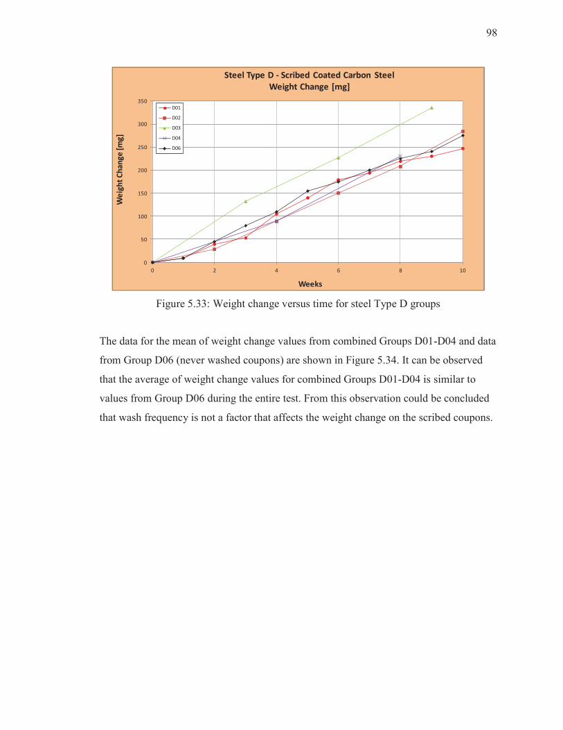
98
Figure 5.33: Weight change versus time for steel Type D groups
The data for the mean of weight change values from combined Groups D01-D04 and data
from Group D06 (never washed coupons) are shown in Figure 5.34. It can be observed
that the average of weight change values for combined Groups D01-D04 is similar to
values from Group D06 during the entire test. From this observation could be concluded
that wash frequency is not a factor that affects the weight change on the scribed coupons.
0
50
100
150
200
250
300
350
0 2 4 6 8 10
We
igh
t C
ha
ng
e [
mg
]
Weeks
Steel Type D - Scribed Coated Carbon Steel
Weight Change [mg]
D01
D02
D03
D04
D06
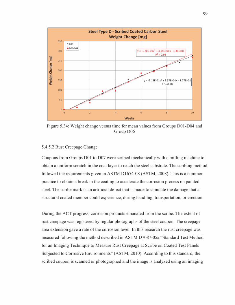
99
y = -5.13E-01x2 + 3.37E+01x - 1.27E+01
R² = 0.98
y = -1.70E-01x2 + 3.14E+01x - 1.31E+01
R² = 0.98
0
50
100
150
200
250
300
350
0 2 4 6 8 10
We
igh
t C
ha
ng
e [
mg]
Weeks
Steel Type D - Scribed Coated Carbon Steel
Weight Change [mg]
D06
D01-D04
Figure 5.34: Weight change versus time for mean values from Groups D01-D04 and
Group D06
5.4.5.2 Rust Creepage Change
Coupons from Groups D01 to D07 were scribed mechanically with a milling machine to
obtain a uniform scratch in the coat layer to reach the steel substrate. The scribing method
followed the requirements given in ASTM D1654-08 (ASTM, 2008). This is a common
practice to obtain a break in the coating to accelerate the corrosion process on painted
steel. The scribe mark is an artificial defect that is made to simulate the damage that a
structural coated member could experience, during handling, transportation, or erection.
During the ACT progress, corrosion products emanated from the scribe. The extent of
rust creepage was registered by regular photographs of the steel coupon. The creepage
area extension gave a rate of the corrosion level. In this research the rust creepage was
measured following the method described in ASTM D7087-05a “Standard Test Method
for an Imaging Technique to Measure Rust Creepage at Scribe on Coated Test Panels
Subjected to Corrosive Environments” (ASTM, 2010). According to this standard, the
scribed coupon is scanned or photographed and the image is analyzed using an imaging
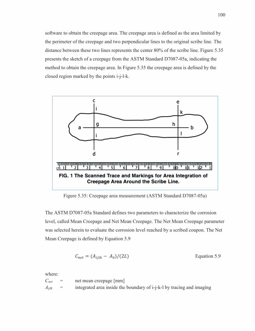
100
software to obtain the creepage area. The creepage area is defined as the area limited by
the perimeter of the creepage and two perpendicular lines to the original scribe line. The
distance between these two lines represents the center 80% of the scribe line. Figure 5.35
presents the sketch of a creepage from the ASTM Standard D7087-05a, indicating the
method to obtain the creepage area. In Figure 5.35 the creepage area is defined by the
closed region marked by the points i-j-l-k.
Figure 5.35: Creepage area measurement (ASTM Standard D7087-05a)
The ASTM D7087-05a Standard defines two parameters to characterize the corrosion
level, called Mean Creepage and Net Mean Creepage. The Net Mean Creepage parameter
was selected herein to evaluate the corrosion level reached by a scribed coupon. The Net
Mean Creepage is defined by Equation 5.9
���� � � !"#$ % '(/�2)( Equation 5.9
where:
Cnet = net mean creepage [mm]
Aijlk = integrated area inside the boundary of i-j-k-l by tracing and imaging
101
A0 = integrated area of scribe line before exposure
L = length of scribe line from which creepage (or undercutting) is extended
and area is integrated.
After the coupons from steel Type D were scribed, they were placed inside the weather
chamber to start the ACT for spot painting evaluation. All coupons were photographed
each week the coupons were washed according to the schedule from Table 5.1. A visual
record of coupons D01-a and D02-b, ordered by weeks and showing the development of
rust creepage is shown in Appendix H. All coupons were photographed each week they
were analyzed and the information was recorded in the research database. Those
photographs were uploaded to AutoCAD 2016 (Autodesk, 2016), a graphical software
that allows the user to edit an image, trace a boundary, and evaluate an area inside a
boundary. Hence, using AutoCAD 2016 (Autodesk, 2016), for each photograph of
scribed coupon, the rust creepage boundary was traced using a closed polyline -a
connected sequence of segments- following the prescription from the ASTM D7087-05a
Standard. Figure 5.36 shows a scribed coupon with the trace of the creepage area using
AutoCAD 2016 (Autodesk, 2016); in the same figure two magnifications from the traced
area are also shown. Coupons from Groups D05 and D07 were photographed until week
4, since at week 6 those coupons were selected to coat their scribes.
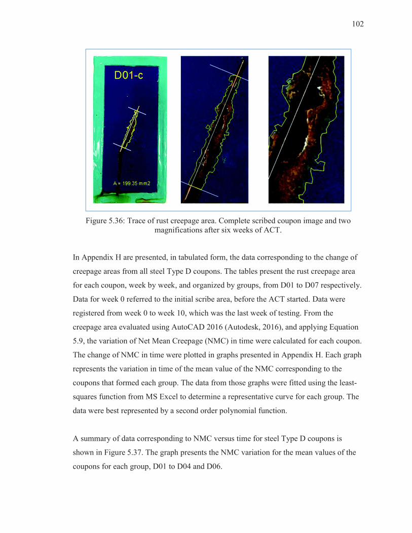
102
Figure 5.36: Trace of rust creepage area. Complete scribed coupon image and two
magnifications after six weeks of ACT.
In Appendix H are presented, in tabulated form, the data corresponding to the change of
creepage areas from all steel Type D coupons. The tables present the rust creepage area
for each coupon, week by week, and organized by groups, from D01 to D07 respectively.
Data for week 0 referred to the initial scribe area, before the ACT started. Data were
registered from week 0 to week 10, which was the last week of testing. From the
creepage area evaluated using AutoCAD 2016 (Autodesk, 2016), and applying Equation
5.9, the variation of Net Mean Creepage (NMC) in time were calculated for each coupon.
The change of NMC in time were plotted in graphs presented in Appendix H. Each graph
represents the variation in time of the mean value of the NMC corresponding to the
coupons that formed each group. The data from those graphs were fitted using the least-
squares function from MS Excel to determine a representative curve for each group. The
data were best represented by a second order polynomial function.
A summary of data corresponding to NMC versus time for steel Type D coupons is
shown in Figure 5.37. The graph presents the NMC variation for the mean values of the
coupons for each group, D01 to D04 and D06.

103
Figure 5.37: Net Mean Creepage versus time for steel Type D groups
From Figure 5.37 can be observed that the curve corresponding to the one-week washing
frequency (Group D01) produces a higher NMC increment than the other groups (Groups
D02 to D04 and D06). Moreover, the no washing alternative (Group D06) shows the
lowest NMC increment for almost the entire test. This pattern was contrary to the
hypothesis of investigation.
Considering as before, that Group D01 had the influence of many wet-dry cycles, data
from this group were discharged. Then, data from Groups D02 to D04 were combined,
averaged, and plotted along with data from the no washing alternative (Group D06), as
shown in Figure 5.38. Analyzing Figure 5.38 it could be concluded that washing a
scribed steel coupon enhances the NMC value. This can be understood as the corrosion
products on a scribe, in some way, helps to protect the scribe from more corrosion, while
washing the scribe enhances the development of more NMC. Therefore, washing a scribe
is not an adequate alternative.
Data from the two plots, Groups D02-D04 and D06 were fitted using the least-squares
function from MS Excel to determine a representative curve for each group. Those fitting
0.0
0.5
1.0
1.5
2.0
0 1 2 3 4 5 6 7 8 9 10
Ne
t M
ea
n C
ree
pa
ge
[m
m]
Weeks
Steel type D - Coated Carbon Steel
Net Mean Creepage [mm]
D01
D02
D03
D04
D06
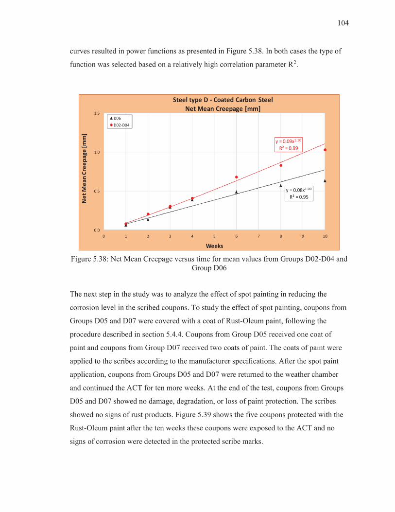
104
curves resulted in power functions as presented in Figure 5.38. In both cases the type of
function was selected based on a relatively high correlation parameter R2.
Figure 5.38: Net Mean Creepage versus time for mean values from Groups D02-D04 and
Group D06
The next step in the study was to analyze the effect of spot painting in reducing the
corrosion level in the scribed coupons. To study the effect of spot painting, coupons from
Groups D05 and D07 were covered with a coat of Rust-Oleum paint, following the
procedure described in section 5.4.4. Coupons from Group D05 received one coat of
paint and coupons from Group D07 received two coats of paint. The coats of paint were
applied to the scribes according to the manufacturer specifications. After the spot paint
application, coupons from Groups D05 and D07 were returned to the weather chamber
and continued the ACT for ten more weeks. At the end of the test, coupons from Groups
D05 and D07 showed no damage, degradation, or loss of paint protection. The scribes
showed no signs of rust products. Figure 5.39 shows the five coupons protected with the
Rust-Oleum paint after the ten weeks these coupons were exposed to the ACT and no
signs of corrosion were detected in the protected scribe marks.
y = 0.08x1.00
R² = 0.95
y = 0.09x1.10
R² = 0.99
0.0
0.5
1.0
1.5
0 1 2 3 4 5 6 7 8 9 10
Ne
t M
ea
n C
ree
pa
ge
[m
m]
Weeks
Steel type D - Coated Carbon Steel
Net Mean Creepage [mm]
D06
D02-D04
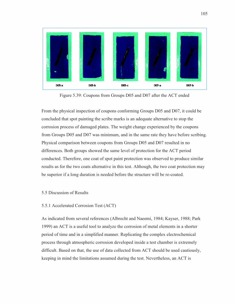
105
Figure 5.39: Coupons from Groups D05 and D07 after the ACT ended
From the physical inspection of coupons conforming Groups D05 and D07, it could be
concluded that spot painting the scribe marks is an adequate alternative to stop the
corrosion process of damaged plates. The weight change experienced by the coupons
from Groups D05 and D07 was minimum, and in the same rate they have before scribing.
Physical comparison between coupons from Groups D05 and D07 resulted in no
differences. Both groups showed the same level of protection for the ACT period
conducted. Therefore, one coat of spot paint protection was observed to produce similar
results as for the two coats alternative in this test. Although, the two coat protection may
be superior if a long duration is needed before the structure will be re-coated.
5.5 Discussion of Results
5.5.1 Accelerated Corrosion Test (ACT)
As indicated from several references (Albrecht and Naeemi, 1984; Kayser, 1988; Park
1999) an ACT is a useful tool to analyze the corrosion of metal elements in a shorter
period of time and in a simplified manner. Replicating the complex electrochemical
process through atmospheric corrosion developed inside a test chamber is extremely
difficult. Based on that, the use of data collected from ACT should be used cautiously,
keeping in mind the limitations assumed during the test. Nevertheless, an ACT is
106
accepted as the best method to perform corrosion analysis under limitations of time and
resources.
In this research the results from the ACT showed a good tendency when analyzed. Some
important assumptions had to be compromised to make adequate use of such a data.
The ACT rapidly produced corrosion effects over the uncoated steel Types (Groups A
and C). The ACT did not produce any appreciable damage to coated steel Type B. From
those results, it can be concluded that the ACT implemented in this study is adequate to
study uncoated pieces of metal but is not suitable for coated elements. Testing coated
elements could require variations in the ACT, such as the application of UV light to
facilitate the deterioration of the coating.
According to specialized literature, weathering steel has a higher resistant to atmospheric
corrosion than carbon steel. During the ACT the coupons from uncoated weathering steel
showed a higher weight increment than uncoated carbon steel. This situation could be
explained based on the fact that during the ACT, the uncoated weathering steel pieces did
not develop the patina protecting layer.
5.5.2 Steel Washing Evaluation
The analysis of ACT results indicated that steel washing is an effective alternative to
reduce the rates of corrosion in steel members. From the data collected, corrosion rates
from the combined washed Groups A02-A05 and C02-C05 demonstrated lower corrosion
rates than results from Groups A10 and C10 corresponding to the no washing
alternatives.
From the results obtained during the ACT on scribed coupons, it can be concluded that
washing spot damage on coated steel members is not an adequate alternative. It was

107
found that the rate of rust creepage area increased when a damaged coated coupon was
subjected to frequent washing.
5.5.3 Spot Painting Evaluation
Painting a small scribe on coated steel members with a simple commercial metal spray
paint product resulted in significant corrosion protection. From the results in this test, the
progression of rust creepage emanating from the scribe was completely eliminated after
the paint cover was applied. The protected scribed coupons did not show any sign of new
corrosion for the remaining time the ACT lasted.
The spot painting test showed that a one-coat application of paint gave similar results
than the two-coat application. However, the use of a two-coat paint protection for spot
damage is recommended to provide adequate long-term protection against corrosion.
108
CORRELATION BETWEEN AN ACCELERATED CORROSION TEST
AND ATMOSPHERIC CORROSION
6.1 Introduction
An accelerated corrosion test (ACT) is a controlled test that seeks to reproduce the
atmospheric corrosion process at the laboratory, in a shorter period of time than at real
environment. Atmospheric corrosion is the result of the combination of several
atmospheric factors that corrode an exposed piece of metal. An ACT seeks to reproduce
the atmospheric corrosion process as accurately as possible, but based on the control of
just a few factors in the laboratory. Based on those limitations, the results obtained from
an ACT should be considered and used with appropriate judgement and discretion.
Nevertheless, an ACT is an appropriate tool to approach the study of real corrosion when
limited by the time and the resources to reproduce actual corrosion process.
In this research, an ACT was developed to reproduce the effect of atmospheric corrosion
on steel coupons under a washing program. The objective of the research was to study the
benefit of steel washing in reducing the corrosion rate of steel highway bridge girders.
Several sets of steel coupons were subjected to different washing frequencies in order to
characterize and model the effect of washing and the frequency of washing in the
reduction of corrosion rates. The ACT process performed in the laboratory and the results
obtained were presented in detail in Chapter 5. In summary, the primary results from the
ACT were the weight change and thickness change of each individual coupon during the
test performance. The weight change was found to be the most accurate parameter to
describe the level of corrosion penetration in a coupon. The weight change resulted in an
increment of weight for the uncoated coupons (steel Types A and C) due to the formation
109
of rust material on the exposed surface. The effect of weight change for coupons from
steel Type B was negligible, and therefore, is not considered in this analysis.
Every week the programmed coupons from steel Types A and C under the ACT were
washed, weighed, and then returned to the chamber. Under this protocol, it was
impossible to measure the corresponding loss of thickness after washing the coupon,
since that action could be done only by cleaning and eliminating all the rust from the
coupon. A cleaned coupon, with all the rust material eliminated, would not be useful to
continue on the ACT, as they were actually used. Therefore, a different set of steel
coupons were required for the ACT to provide a relationship between the weight
increment in steel coupons during the ACT with the corresponding level of corrosion
penetration. Also, this new set of coupons subjected to the ACT should offer enough
information in order to properly apply the results from the ACT to the study of real
problems. Those expected relationships are enounced in the following:
a) A relationship was required to obtain the actual level of corrosion corresponding to
each amount of weight increment of a coupon inside the chamber. This relationship
should correlate each value of weight increment to the corresponding level of
corrosion during the ACT, and consequently, the corresponding amount of corrosion
penetration in the steel coupon.
b) A relationship between a unit time in the chamber during the ACT and the
corresponding time for a real environment. This will be useful in order to correlate
the results obtained from the ACT to real problems.
c) A relationship to extrapolate the results from the ACT during a short period of time to
real problems of larger periods of time, such as the bridge service life.
To achieve all these required relationships, it was necessary to perform an ACT to a new
group of steel coupons. The new ACT was named “Control Test”, and the details of the
tested coupons, the test protocol, and the results obtained are presented in the next
sections.
110
6.2 Control Test
The Control Test was an ACT performed using a new series of steel coupons, from steel
Types A and C, in order to develop the necessary relationships between the results from
an ACT and the corrosion occurring in a real environment.
6.2.1 Number of Coupons and Identification
The Control Test was designed to expose a set of steel coupons to an ACT and to
measure the increment of weight and the thickness loss experienced by the coupons under
the test. Steel coupons in the Control Test were exposed to an ACT, and at a certain
frequency, a group of coupons were withdrawn from the chamber to be analyzed.
Five groups of coupons were assembled for each type of steel to be tested (steel Types A
and C). The groups of coupons from steel Type A were identified from X01 to X05,
while groups from steel Type C were identified from W01 to W05. To seek better
confidence in the mean results, three coupons were used for each group. The
identification for all control group coupons considered in this test are described in
Appendix I. All coupons tested during the Control Test were protected with an epoxy
coat to expose only one surface for corrosion development, similar to the coupons tested
in the ACT for steel washing evaluation.
6.2.2 Schedule for Control Test
The Control Test was designed to analyze each group at a bi-weekly frequency. Thus,
each two weeks a group of coupons from each steel type was withdrawn from the
chamber for analysis. At week 2, the groups designated with number 01 (X01 and W01)
were analyzed as explained in the next sections. At week 4 the groups numbered 02 (X02
and W02) were analyzed, and in the same way, until groups numbered 05 (X05 and W05)
were analyzed at week number 10.
111
6.2.3 Initial Data Acquisition
The initial physical characteristics from each coupon were taken and registered before the
beginning of the Control Test. The weight and a photography from each steel coupon
were registered. All coupons were weighed using the electronic balance; the
measurement was repeated three times for a better precision. Each steel coupon was
photographed using the digital camera from a smartphone. The initial weight of each
coupon, identified as the weight at week 0, is shown in Appendix I. The photographs
from all coupons before the Control Test started were registered as part of the research
database. In Appendix I a few selected photographs from coupons before the Control Test
started are shown.
6.2.4 Procedure for the Control Test
The five groups of steel coupons from steel Types A and C respectively were supported
on racks and placed inside the weather chamber for an ACT. This test followed almost
the same process that followed the ACT for steel washing evaluation. The coupons were
exposed to a cyclic spray process, every day during ten weeks, using the same type of
sodium chloride solution (NaCl) at 5% by weight. In this test the bi-weekly selected
coupons were not power washed but were cleaned by sandblasting to eliminate all of the
excess material from the corroded surfaces. The protocol followed in this Control Test is
detailed in the next sections.
6.2.4.1 Data before Sandblasting
After removal from the chamber the selected coupons were air-dried and weighed. The
weight from each coupon was registered in a master spreadsheet for subsequent
calculations. The registered weights are presented in Appendix I. Then, a photograph
from each selected coupon was captured, to record its corroded condition. All
photographs were registered in the research database. The photographs from selected
groups of coupons are shown in Appendix I.

112
6.2.4.2 Sandblasting
To eliminate all corrosion material from a corroded coupon a mechanical process was
employed. Following the ASTM G1-03 “Standard Practice for Preparing, Cleaning, and
Evaluating Corrosion Test Specimens” (ASTM, 2011), a sandblasting method was used.
An abrasive blast cabinet from the Bowen Laboratory at Purdue was used to remove the
corrosion products from the coupon. During the sandblasting process, proper care was
exercised to eliminate only the corrosion products, and avoided the removal of any base
metal.
6.2.4.3 Data after Sandblasting
The tested coupons after sandblasting were weighed and photographed. The final weights
were recorded in the master spreadsheet. The weights after sandblasting corresponding to
all the coupons are presented in tables in Appendix I, classified by steel types and by
groups. The photographs after sandblasting were also recorded in the research database.
As before, selected photographs corresponding to some groups of coupons after
sandblasting are provided in Appendix I.
6.2.5 Results from Control Test
The mean values of the weight change, measured bi-weekly, of the tree coupons that
conformed each group of steel Type A (uncoated carbon steel) are shown in Table 6.1.
As indicated previously, at week 2 the coupons from Group X01 were tested, at week 4
the Group X02 was tested, until week 10 when the coupons from Group X05 were tested.
The weight increment due to corrosion during control test was registered before the
sandblasting work, and the weight loss due to cleaning the corroded surface was
registered after the sandblasting was performed. The weight increment and weight loss
are presented in absolute values and as value per unit of exposed area. The normalized
weight increment and loss values were calculated considering an exposed surface of 2.5
in. (63.5 mm) by 5.5 in. (139.7 mm) as shown in Figure 6.1.
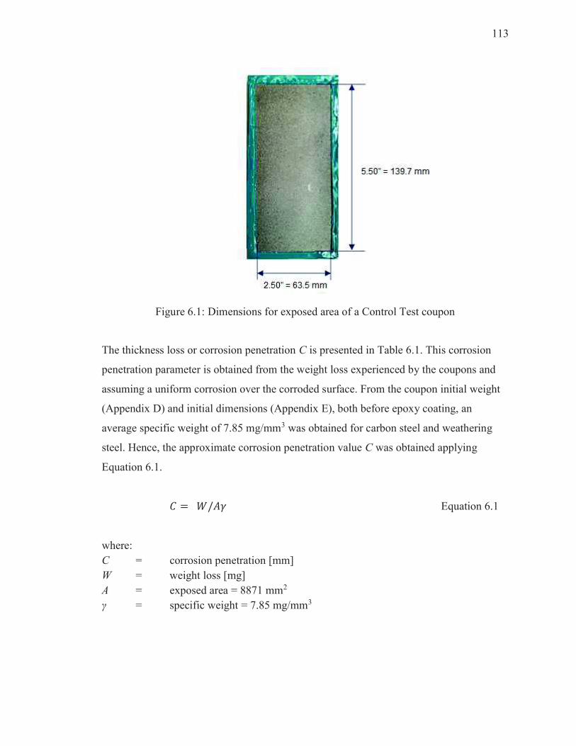
113
Figure 6.1: Dimensions for exposed area of a Control Test coupon
The thickness loss or corrosion penetration C is presented in Table 6.1. This corrosion
penetration parameter is obtained from the weight loss experienced by the coupons and
assuming a uniform corrosion over the corroded surface. From the coupon initial weight
(Appendix D) and initial dimensions (Appendix E), both before epoxy coating, an
average specific weight of 7.85 mg/mm3 was obtained for carbon steel and weathering
steel. Hence, the approximate corrosion penetration value C was obtained applying
Equation 6.1.
� � �/�� Equation 6.1
where:
C = corrosion penetration [mm]
W = weight loss [mg]
A = exposed area = 8871 mm2
γ = specific weight = 7.85 mg/mm3
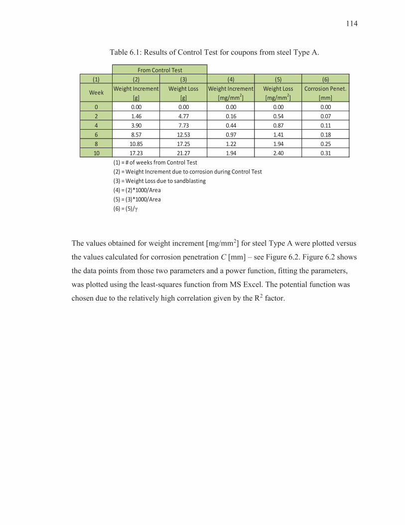
114
Table 6.1: Results of Control Test for coupons from steel Type A.
(1) (2) (3) (4) (5) (6)
Weight Increment Weight Loss Weight Increment Weight Loss Corrosion Penet.
[g] [g] [mg/mm2] [mg/mm
2] [mm]
0 0.00 0.00 0.00 0.00 0.00
2 1.46 4.77 0.16 0.54 0.07
4 3.90 7.73 0.44 0.87 0.11
6 8.57 12.53 0.97 1.41 0.18
8 10.85 17.25 1.22 1.94 0.25
10 17.23 21.27 1.94 2.40 0.31
(1) = # of weeks from Control Test
(2) = Weight Increment due to corrosion during Control Test
(3) = Weight Loss due to sandblasting
(4) = (2)*1000/Area
(5) = (3)*1000/Area
(6) = (5)/γ
Week
From Control Test
The values obtained for weight increment [mg/mm2] for steel Type A were plotted versus
the values calculated for corrosion penetration C [mm] – see Figure 6.2. Figure 6.2 shows
the data points from those two parameters and a power function, fitting the parameters,
was plotted using the least-squares function from MS Excel. The potential function was
chosen due to the relatively high correlation given by the R2 factor.
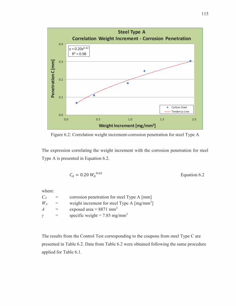
115
y = 0.20x0.62
R² = 0.98
0.0
0.1
0.2
0.3
0.4
0.0 0.5 1.0 1.5 2.0
Pe
ne
tra
tio
n C
[m
m]
Weight Increment [mg/mm2]
Steel Type A
Correlation Weight Increment - Corrosion Penetration
Carbon Steel
Tendency Line
Figure 6.2: Correlation weight increment-corrosion penetration for steel Type A
The expression correlating the weight increment with the corrosion penetration for steel
Type A is presented in Equation 6.2.
�� � 0.20 ��
�. ! Equation 6.2
where:
CA = corrosion penetration for steel Type A [mm]
WA = weight increment for steel Type A [mg/mm2]
A = exposed area = 8871 mm2
γ = specific weight = 7.85 mg/mm3
The results from the Control Test corresponding to the coupons from steel Type C are
presented in Table 6.2. Data from Table 6.2 were obtained following the same procedure
applied for Table 6.1.
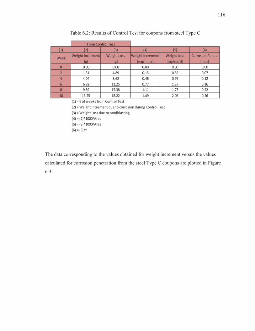
116
Table 6.2: Results of Control Test for coupons from steel Type C
(1) (2) (3) (4) (5) (6)
Weight Increment Weight Loss Weight Increment Weight Loss Corrosion Penet.
[g] [g] [mg/mm2] [mg/mm2] [mm]
0 0.00 0.00 0.00 0.00 0.00
2 1.31 4.89 0.15 0.55 0.07
4 4.04 8.62 0.46 0.97 0.12
6 6.82 11.25 0.77 1.27 0.16
8 9.89 15.38 1.11 1.73 0.22
10 13.25 18.22 1.49 2.05 0.26
(1) = # of weeks from Control Test
(2) = Weight Increment due to corrosion during Control Test
(3) = Weight Loss due to sandblasting
(4) = (2)*1000/Area
(5) = (3)*1000/Area
(6) = (5)/γ
From Control Test
Week
The data corresponding to the values obtained for weight increment versus the values
calculated for corrosion penetration from the steel Type C coupons are plotted in Figure
6.3.
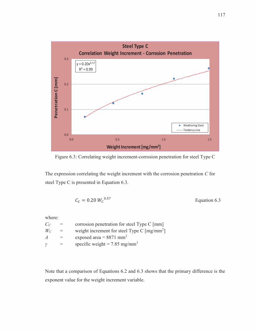
117
y = 0.20x0.57
R² = 0.99
0.0
0.1
0.2
0.3
0.0 0.5 1.0 1.5
Pe
ne
tra
tio
n C
[m
m]
Weight Increment [mg/mm2]
Steel Type C
Correlation Weight Increment - Corrosion Penetration
Weathering Steel
Tendency Line
Figure 6.3: Correlating weight increment-corrosion penetration for steel Type C
The expression correlating the weight increment with the corrosion penetration C for
steel Type C is presented in Equation 6.3.
�� � 0.20 ��
�. ! Equation 6.3
where:
CC = corrosion penetration for steel Type C [mm]
WC = weight increment for steel Type C [mg/mm2]
A = exposed area = 8871 mm2
γ = specific weight = 7.85 mg/mm3
Note that a comparison of Equations 6.2 and 6.3 shows that the primary difference is the
exponent value for the weight increment variable.
118
6.3 Correlation between ACT and Atmospheric Corrosion
The results from the Control Test, together with the data obtained during the ACT for
steel washing evaluation were used to evaluate the length of time to develop corrosion
penetration. The linkage to corrosion for real environments was based on the studies from
Albrecht and Naeemi (1984) and Kayser (1988). The correlation expressions are provided
in the following sections.
6.3.1 Correlation between the Weight Increment and Corrosion Penetration during ACT
The first step was to obtain the corrosion penetration values during the ACT for steel
coupons from washing evaluation for the twenty four weeks the test lasted. To obtain the
corrosion penetration values, Equations 6.2 and 6.3 were used for steel Type A and C
respectively, and the results are presented in Tables 6.3 and 6.4.
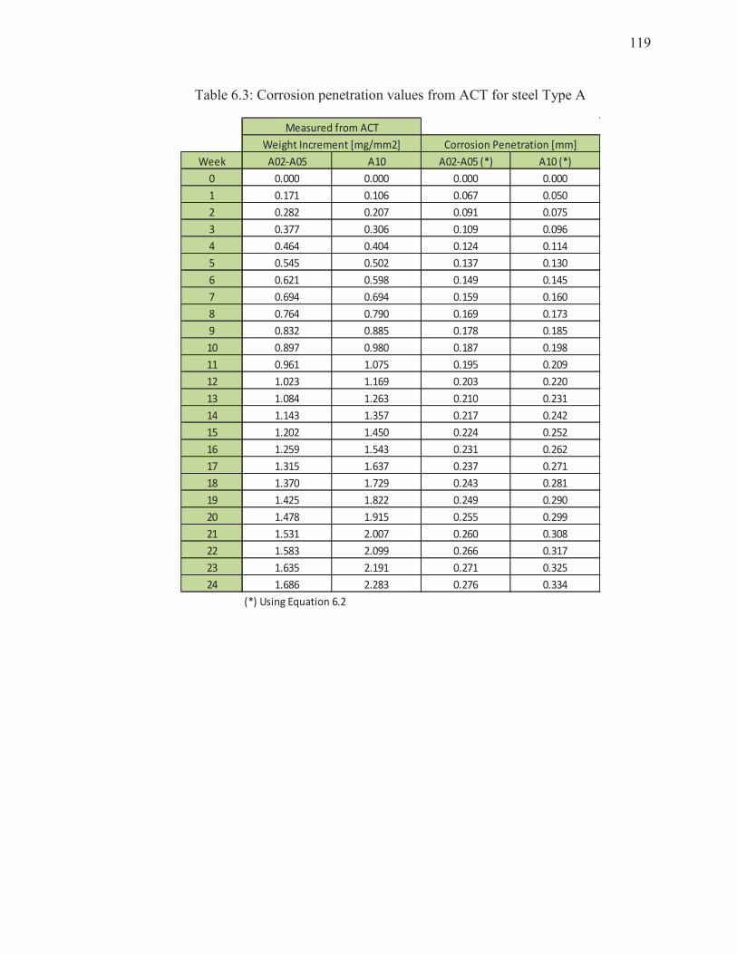
119
Table 6.3: Corrosion penetration values from ACT for steel Type A
Week A02-A05 A10 A02-A05 (*) A10 (*)
0 0.000 0.000 0.000 0.000
1 0.171 0.106 0.067 0.050
2 0.282 0.207 0.091 0.075
3 0.377 0.306 0.109 0.096
4 0.464 0.404 0.124 0.114
5 0.545 0.502 0.137 0.130
6 0.621 0.598 0.149 0.145
7 0.694 0.694 0.159 0.160
8 0.764 0.790 0.169 0.173
9 0.832 0.885 0.178 0.185
10 0.897 0.980 0.187 0.198
11 0.961 1.075 0.195 0.209
12 1.023 1.169 0.203 0.220
13 1.084 1.263 0.210 0.231
14 1.143 1.357 0.217 0.242
15 1.202 1.450 0.224 0.252
16 1.259 1.543 0.231 0.262
17 1.315 1.637 0.237 0.271
18 1.370 1.729 0.243 0.281
19 1.425 1.822 0.249 0.290
20 1.478 1.915 0.255 0.299
21 1.531 2.007 0.260 0.308
22 1.583 2.099 0.266 0.317
23 1.635 2.191 0.271 0.325
24 1.686 2.283 0.276 0.334
(*) Using Equation 6.2
Weight Increment [mg/mm2] Corrosion Penetration [mm]
Measured from ACT
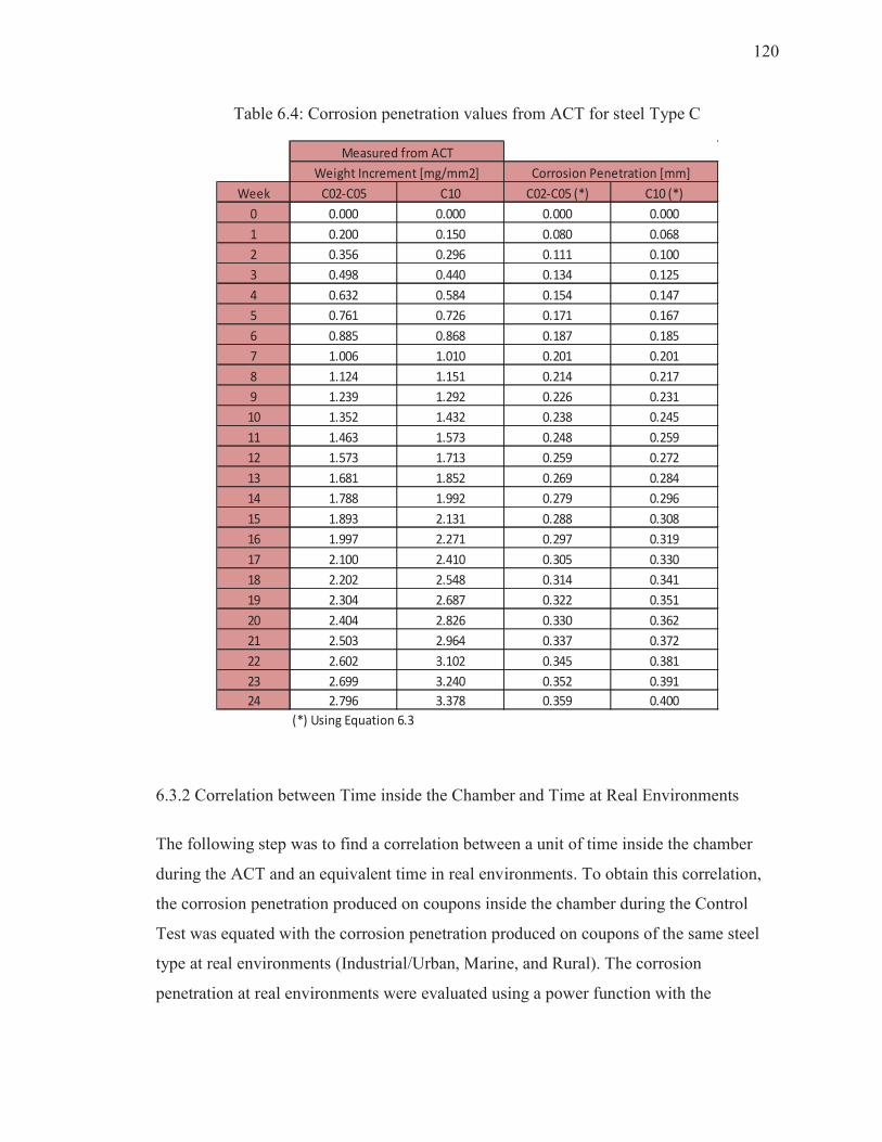
120
Table 6.4: Corrosion penetration values from ACT for steel Type C
Week C02-C05 C10 C02-C05 (*) C10 (*)
0 0.000 0.000 0.000 0.000
1 0.200 0.150 0.080 0.068
2 0.356 0.296 0.111 0.100
3 0.498 0.440 0.134 0.125
4 0.632 0.584 0.154 0.147
5 0.761 0.726 0.171 0.167
6 0.885 0.868 0.187 0.185
7 1.006 1.010 0.201 0.201
8 1.124 1.151 0.214 0.217
9 1.239 1.292 0.226 0.231
10 1.352 1.432 0.238 0.245
11 1.463 1.573 0.248 0.259
12 1.573 1.713 0.259 0.272
13 1.681 1.852 0.269 0.284
14 1.788 1.992 0.279 0.296
15 1.893 2.131 0.288 0.308
16 1.997 2.271 0.297 0.319
17 2.100 2.410 0.305 0.330
18 2.202 2.548 0.314 0.341
19 2.304 2.687 0.322 0.351
20 2.404 2.826 0.330 0.362
21 2.503 2.964 0.337 0.372
22 2.602 3.102 0.345 0.381
23 2.699 3.240 0.352 0.391
24 2.796 3.378 0.359 0.400
(*) Using Equation 6.3
Measured from ACT
Weight Increment [mg/mm2] Corrosion Penetration [mm]
6.3.2 Correlation between Time inside the Chamber and Time at Real Environments
The following step was to find a correlation between a unit of time inside the chamber
during the ACT and an equivalent time in real environments. To obtain this correlation,
the corrosion penetration produced on coupons inside the chamber during the Control
Test was equated with the corrosion penetration produced on coupons of the same steel
type at real environments (Industrial/Urban, Marine, and Rural). The corrosion
penetration at real environments were evaluated using a power function with the
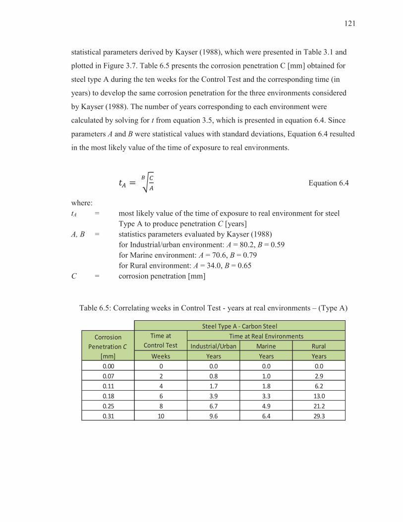
121
statistical parameters derived by Kayser (1988), which were presented in Table 3.1 and
plotted in Figure 3.7. Table 6.5 presents the corrosion penetration C [mm] obtained for
steel type A during the ten weeks for the Control Test and the corresponding time (in
years) to develop the same corrosion penetration for the three environments considered
by Kayser (1988). The number of years corresponding to each environment were
calculated by solving for t from equation 3.5, which is presented in equation 6.4. Since
parameters A and B were statistical values with standard deviations, Equation 6.4 resulted
in the most likely value of the time of exposure to real environments.
�� � ���
Equation 6.4
where:
tA = most likely value of the time of exposure to real environment for steel
Type A to produce penetration C [years]
A, B = statistics parameters evaluated by Kayser (1988)
for Industrial/urban environment: A = 80.2, B = 0.59
for Marine environment: A = 70.6, B = 0.79
for Rural environment: A = 34.0, B = 0.65
C = corrosion penetration [mm]
Table 6.5: Correlating weeks in Control Test - years at real environments – (Type A)
Industrial/Urban Marine Rural
Weeks Years Years Years
0.00 0 0.0 0.0 0.0
0.07 2 0.8 1.0 2.9
0.11 4 1.7 1.8 6.2
0.18 6 3.9 3.3 13.0
0.25 8 6.7 4.9 21.2
0.31 10 9.6 6.4 29.3
Time at Real EnvironmentsTime at
Control TestCorrosion
Penetration C
[mm]
Steel Type A - Carbon Steel
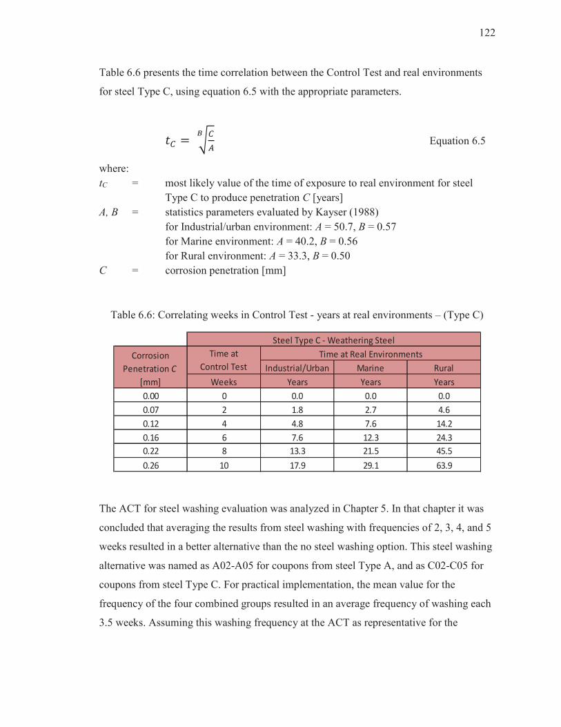
122
Table 6.6 presents the time correlation between the Control Test and real environments
for steel Type C, using equation 6.5 with the appropriate parameters.
�� � ��
�
Equation 6.5
where:
tC = most likely value of the time of exposure to real environment for steel
Type C to produce penetration C [years]
A, B = statistics parameters evaluated by Kayser (1988)
for Industrial/urban environment: A = 50.7, B = 0.57
for Marine environment: A = 40.2, B = 0.56
for Rural environment: A = 33.3, B = 0.50
C = corrosion penetration [mm]
Table 6.6: Correlating weeks in Control Test - years at real environments – (Type C)
Industrial/Urban Marine Rural
Weeks Years Years Years
0.00 0 0.0 0.0 0.0
0.07 2 1.8 2.7 4.6
0.12 4 4.8 7.6 14.2
0.16 6 7.6 12.3 24.3
0.22 8 13.3 21.5 45.5
0.26 10 17.9 29.1 63.9
Steel Type C - Weathering Steel
Corrosion
Penetration C
[mm]
Time at
Control Test
Time at Real Environments
The ACT for steel washing evaluation was analyzed in Chapter 5. In that chapter it was
concluded that averaging the results from steel washing with frequencies of 2, 3, 4, and 5
weeks resulted in a better alternative than the no steel washing option. This steel washing
alternative was named as A02-A05 for coupons from steel Type A, and as C02-C05 for
coupons from steel Type C. For practical implementation, the mean value for the
frequency of the four combined groups resulted in an average frequency of washing each
3.5 weeks. Assuming this washing frequency at the ACT as representative for the
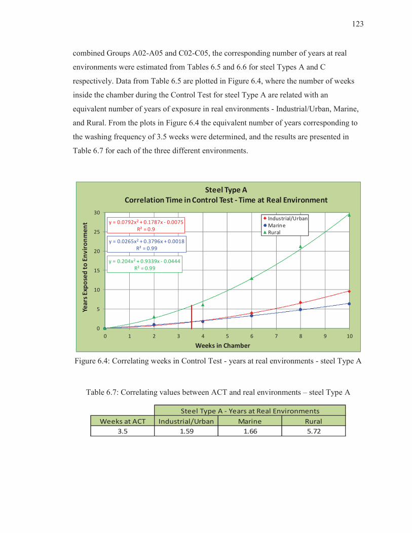
123
combined Groups A02-A05 and C02-C05, the corresponding number of years at real
environments were estimated from Tables 6.5 and 6.6 for steel Types A and C
respectively. Data from Table 6.5 are plotted in Figure 6.4, where the number of weeks
inside the chamber during the Control Test for steel Type A are related with an
equivalent number of years of exposure in real environments - Industrial/Urban, Marine,
and Rural. From the plots in Figure 6.4 the equivalent number of years corresponding to
the washing frequency of 3.5 weeks were determined, and the results are presented in
Table 6.7 for each of the three different environments.
y = 0.0792x2 + 0.1787x - 0.0075
R² = 0.9
y = 0.0265x2 + 0.3796x + 0.0018
R² = 0.99
y = 0.204x2 + 0.9339x - 0.0444
R² = 0.99
0
5
10
15
20
25
30
0 1 2 3 4 5 6 7 8 9 10
Yea
rs E
xpo
sed
to
En
vir
on
me
nt
Weeks in Chamber
Steel Type A
Correlation Time in Control Test - Time at Real Environment
Industrial/Urban
Marine
Rural
Figure 6.4: Correlating weeks in Control Test - years at real environments - steel Type A
Table 6.7: Correlating values between ACT and real environments – steel Type A
Weeks at ACT Industrial/Urban Marine Rural
3.5 1.59 1.66 5.72
Steel Type A - Years at Real Environments
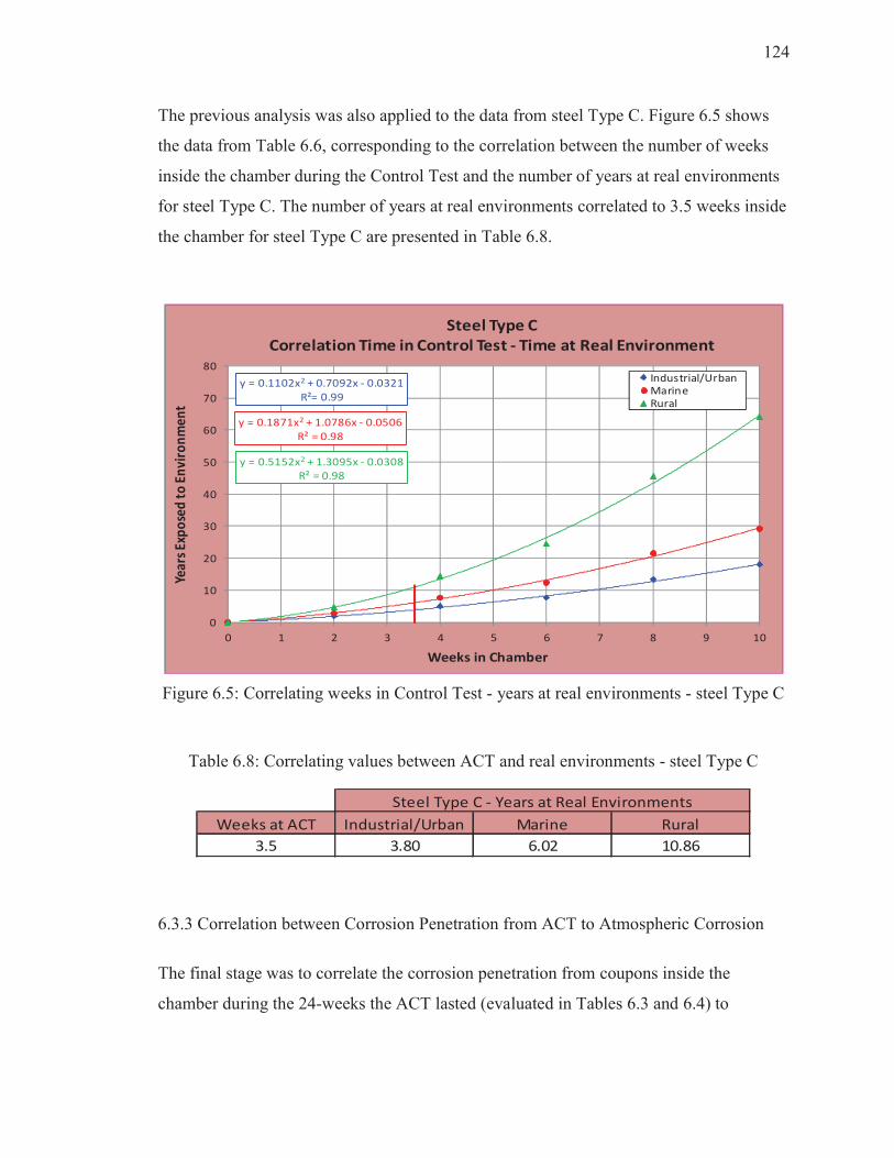
124
The previous analysis was also applied to the data from steel Type C. Figure 6.5 shows
the data from Table 6.6, corresponding to the correlation between the number of weeks
inside the chamber during the Control Test and the number of years at real environments
for steel Type C. The number of years at real environments correlated to 3.5 weeks inside
the chamber for steel Type C are presented in Table 6.8.
y = 0.1102x2 + 0.7092x - 0.0321
R²= 0.99
y = 0.1871x2 + 1.0786x - 0.0506
R² = 0.98
y = 0.5152x2 + 1.3095x - 0.0308
R² = 0.98
0
10
20
30
40
50
60
70
80
0 1 2 3 4 5 6 7 8 9 10
Yea
rs E
xpo
sed
to
En
viro
nm
en
t
Weeks in Chamber
Steel Type C
Correlation Time in Control Test - Time at Real Environment
Industrial/UrbanMarineRural
Figure 6.5: Correlating weeks in Control Test - years at real environments - steel Type C
Table 6.8: Correlating values between ACT and real environments - steel Type C
6.3.3 Correlation between Corrosion Penetration from ACT to Atmospheric Corrosion
The final stage was to correlate the corrosion penetration from coupons inside the
chamber during the 24-weeks the ACT lasted (evaluated in Tables 6.3 and 6.4) to
Weeks at ACT Industrial/Urban Marine Rural
3.5 3.80 6.02 10.86
Steel Type C - Years at Real Environments
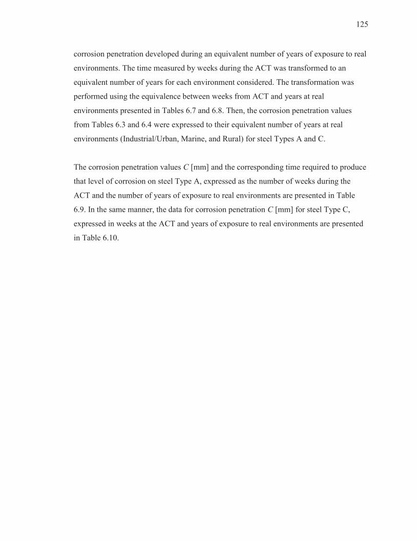
125
corrosion penetration developed during an equivalent number of years of exposure to real
environments. The time measured by weeks during the ACT was transformed to an
equivalent number of years for each environment considered. The transformation was
performed using the equivalence between weeks from ACT and years at real
environments presented in Tables 6.7 and 6.8. Then, the corrosion penetration values
from Tables 6.3 and 6.4 were expressed to their equivalent number of years at real
environments (Industrial/Urban, Marine, and Rural) for steel Types A and C.
The corrosion penetration values C [mm] and the corresponding time required to produce
that level of corrosion on steel Type A, expressed as the number of weeks during the
ACT and the number of years of exposure to real environments are presented in Table
6.9. In the same manner, the data for corrosion penetration C [mm] for steel Type C,
expressed in weeks at the ACT and years of exposure to real environments are presented
in Table 6.10.
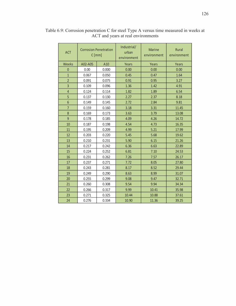
126
Table 6.9: Corrosion penetration C for steel Type A versus time measured in weeks at ACT and years at real environments
Weeks A02-A05 A10 Years Years Years
0 0.00 0.000 0.00 0.00 0.00
1 0.067 0.050 0.45 0.47 1.64
2 0.091 0.075 0.91 0.95 3.27
3 0.109 0.096 1.36 1.42 4.91
4 0.124 0.114 1.82 1.89 6.54
5 0.137 0.130 2.27 2.37 8.18
6 0.149 0.145 2.72 2.84 9.81
7 0.159 0.160 3.18 3.31 11.45
8 0.169 0.173 3.63 3.79 13.08
9 0.178 0.185 4.09 4.26 14.72
10 0.187 0.198 4.54 4.73 16.35
11 0.195 0.209 4.99 5.21 17.99
12 0.203 0.220 5.45 5.68 19.62
13 0.210 0.231 5.90 6.15 21.26
14 0.217 0.242 6.36 6.63 22.89
15 0.224 0.252 6.81 7.10 24.53
16 0.231 0.262 7.26 7.57 26.17
17 0.237 0.271 7.72 8.05 27.80
18 0.243 0.281 8.17 8.52 29.44
19 0.249 0.290 8.63 8.99 31.07
20 0.255 0.299 9.08 9.47 32.71
21 0.260 0.308 9.54 9.94 34.34
22 0.266 0.317 9.99 10.41 35.98
23 0.271 0.325 10.44 10.88 37.61
24 0.276 0.334 10.90 11.36 39.25
ACTCorrosion Penetration
C [mm]
Industrial/
urban
environment
Marine
environment
Rural
environment
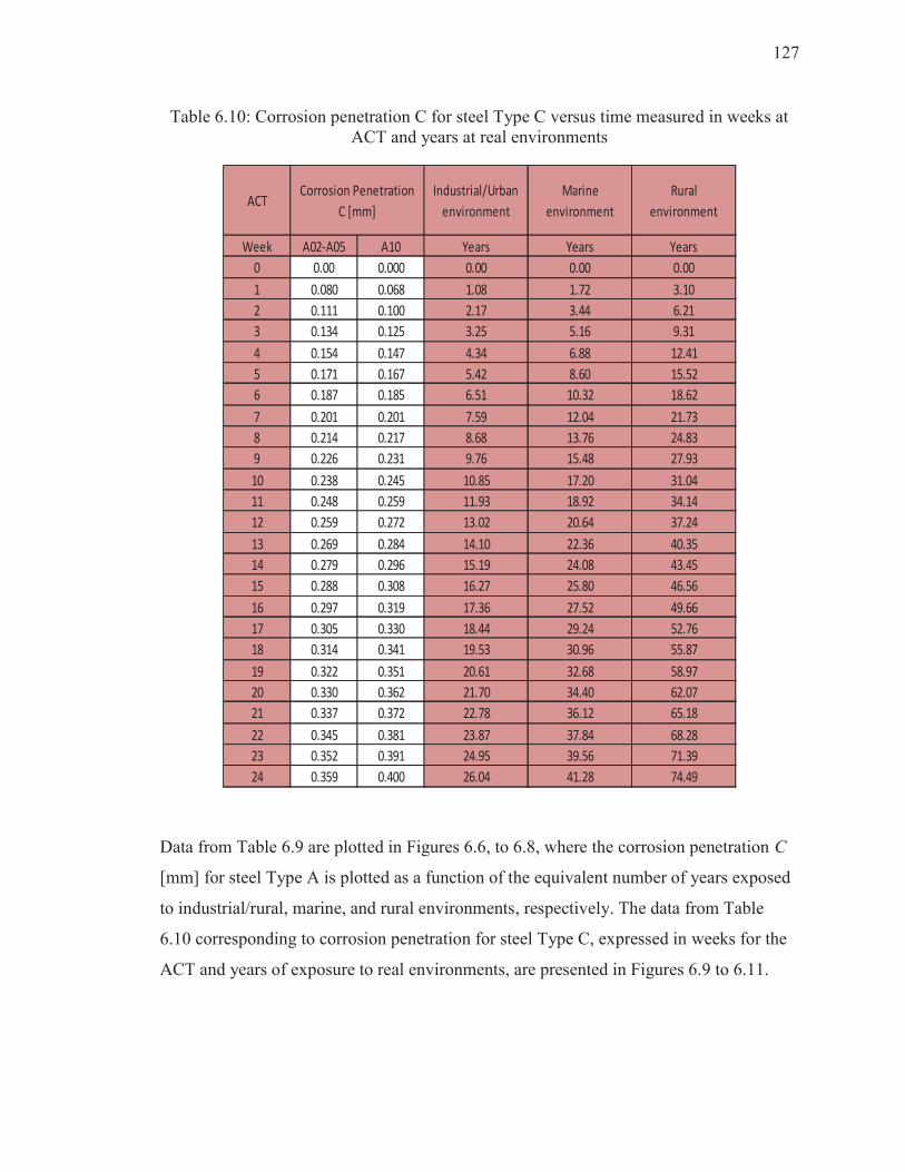
127
Table 6.10: Corrosion penetration C for steel Type C versus time measured in weeks at ACT and years at real environments
Week A02-A05 A10 Years Years Years
0 0.00 0.000 0.00 0.00 0.00
1 0.080 0.068 1.08 1.72 3.10
2 0.111 0.100 2.17 3.44 6.21
3 0.134 0.125 3.25 5.16 9.31
4 0.154 0.147 4.34 6.88 12.41
5 0.171 0.167 5.42 8.60 15.52
6 0.187 0.185 6.51 10.32 18.62
7 0.201 0.201 7.59 12.04 21.73
8 0.214 0.217 8.68 13.76 24.83
9 0.226 0.231 9.76 15.48 27.93
10 0.238 0.245 10.85 17.20 31.04
11 0.248 0.259 11.93 18.92 34.14
12 0.259 0.272 13.02 20.64 37.24
13 0.269 0.284 14.10 22.36 40.35
14 0.279 0.296 15.19 24.08 43.45
15 0.288 0.308 16.27 25.80 46.56
16 0.297 0.319 17.36 27.52 49.66
17 0.305 0.330 18.44 29.24 52.76
18 0.314 0.341 19.53 30.96 55.87
19 0.322 0.351 20.61 32.68 58.97
20 0.330 0.362 21.70 34.40 62.07
21 0.337 0.372 22.78 36.12 65.18
22 0.345 0.381 23.87 37.84 68.28
23 0.352 0.391 24.95 39.56 71.39
24 0.359 0.400 26.04 41.28 74.49
ACTIndustrial/Urban
environment
Corrosion Penetration
C [mm]
Marine
environment
Rural
environment
Data from Table 6.9 are plotted in Figures 6.6, to 6.8, where the corrosion penetration C
[mm] for steel Type A is plotted as a function of the equivalent number of years exposed
to industrial/rural, marine, and rural environments, respectively. The data from Table
6.10 corresponding to corrosion penetration for steel Type C, expressed in weeks for the
ACT and years of exposure to real environments, are presented in Figures 6.9 to 6.11.

128
y = 0.10x0.45
y = 0.08x0.60
0.0
0.1
0.2
0.3
0.4
0.0 2.0 4.0 6.0 8.0 10.0 12.0
Pe
ne
tra
tio
n C
[m
m]
Years
Steel Type A - Industrial/Urban
Corrosion Penetration
A02-A05
A10
Figure 6.6: Corrosion penetration vs. time - steel Type A - Industrial/Urban environment
y = 0.09x0.45
y = 0.08x0.60
0.0
0.1
0.2
0.3
0.4
0.0 2.0 4.0 6.0 8.0 10.0 12.0
Pe
ne
tra
tio
n C
[m
m]
Years
Steel Type A - Marine
Corrosion Penetration
A02-A05
A10
Figure 6.7: Corrosion penetration vs. time - steel Type A - Marine environment
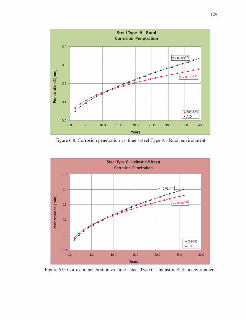
129
y = 0.05x0.45
y = 0.04x0.60
0.0
0.1
0.2
0.3
0.4
0.0 5.0 10.0 15.0 20.0 25.0 30.0 35.0 40.0
Pe
ne
tra
tio
n C
[m
m]
Years
Steel Type A - Rural
Corrosion Penetration
A02-A05
A10
Figure 6.8: Corrosion penetration vs. time - steel Type A - Rural environment
y = 0.08x0.47
y = 0.06x0.56
0.0
0.1
0.2
0.3
0.4
0.5
0.0 5.0 10.0 15.0 20.0 25.0 30.0
Pe
ne
tra
tio
n C
[m
m]
Years
Steel Type C - Industrial/Urban
Corrosion Penetration
C02-C05
C10
Figure 6.9: Corrosion penetration vs. time - steel Type C - Industrial/Urban environment
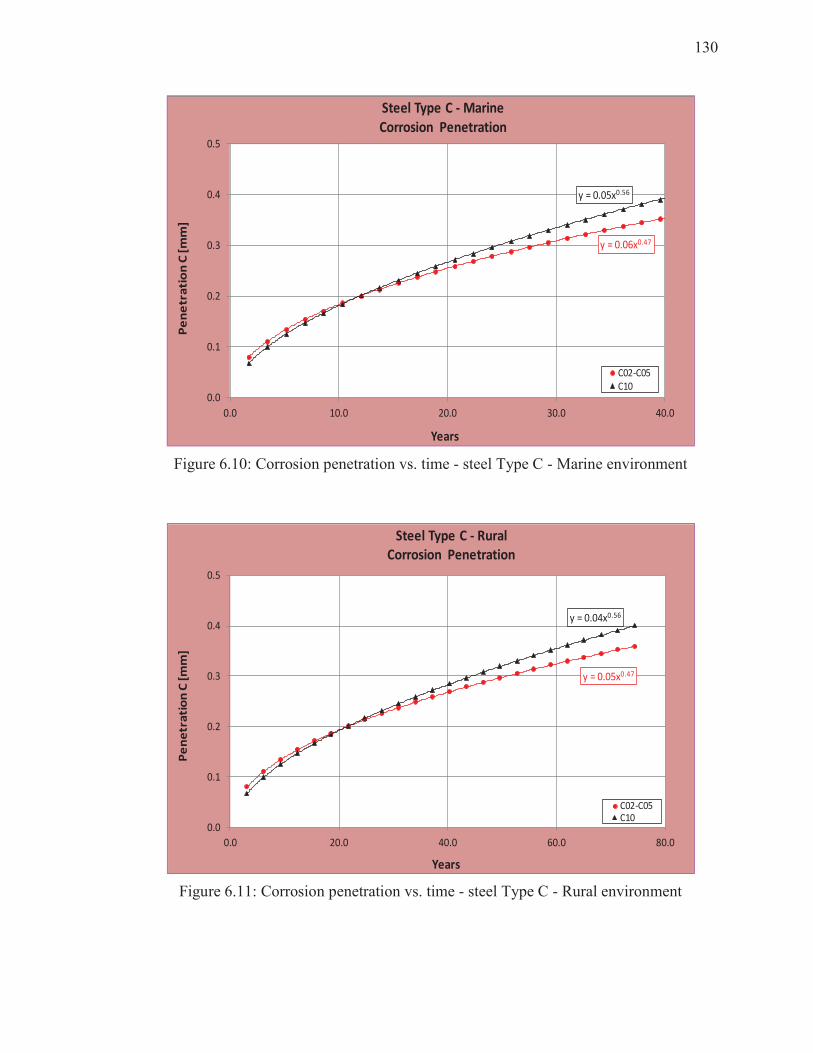
130
y = 0.06x0.47
y = 0.05x0.56
0.0
0.1
0.2
0.3
0.4
0.5
0.0 10.0 20.0 30.0 40.0
Pe
ne
tra
tio
n C
[m
m]
Years
Steel Type C - Marine
Corrosion Penetration
C02-C05
C10
Figure 6.10: Corrosion penetration vs. time - steel Type C - Marine environment
y = 0.05x0.47
y = 0.04x0.56
0.0
0.1
0.2
0.3
0.4
0.5
0.0 20.0 40.0 60.0 80.0
Pe
ne
tra
tio
n C
[m
m]
Years
Steel Type C - Rural
Corrosion Penetration
C02-C05C10
Figure 6.11: Corrosion penetration vs. time - steel Type C - Rural environment
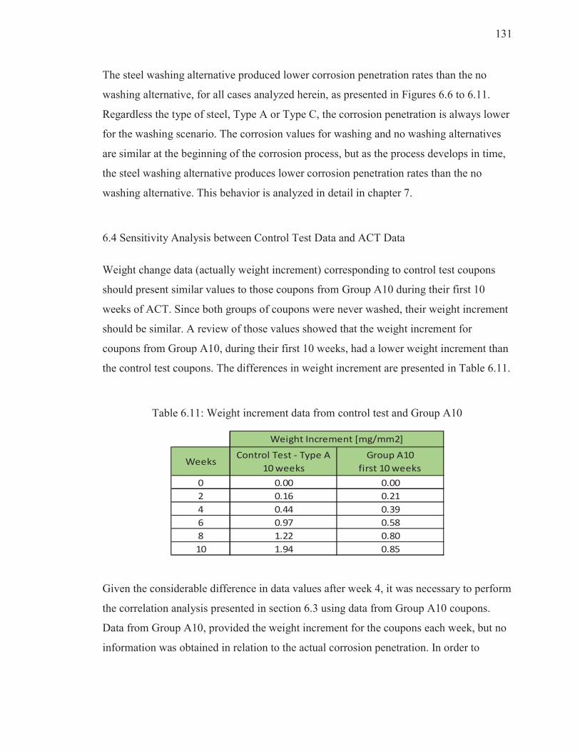
131
The steel washing alternative produced lower corrosion penetration rates than the no
washing alternative, for all cases analyzed herein, as presented in Figures 6.6 to 6.11.
Regardless the type of steel, Type A or Type C, the corrosion penetration is always lower
for the washing scenario. The corrosion values for washing and no washing alternatives
are similar at the beginning of the corrosion process, but as the process develops in time,
the steel washing alternative produces lower corrosion penetration rates than the no
washing alternative. This behavior is analyzed in detail in chapter 7.
6.4 Sensitivity Analysis between Control Test Data and ACT Data
Weight change data (actually weight increment) corresponding to control test coupons
should present similar values to those coupons from Group A10 during their first 10
weeks of ACT. Since both groups of coupons were never washed, their weight increment
should be similar. A review of those values showed that the weight increment for
coupons from Group A10, during their first 10 weeks, had a lower weight increment than
the control test coupons. The differences in weight increment are presented in Table 6.11.
Table 6.11: Weight increment data from control test and Group A10
0 0.00 0.00
2 0.16 0.21
4 0.44 0.39
6 0.97 0.58
8 1.22 0.80
10 1.94 0.85
Control Test - Type A
10 weeks
Group A10
first 10 weeksWeeks
Weight Increment [mg/mm2]
Given the considerable difference in data values after week 4, it was necessary to perform
the correlation analysis presented in section 6.3 using data from Group A10 coupons.
Data from Group A10, provided the weight increment for the coupons each week, but no
information was obtained in relation to the actual corrosion penetration. In order to
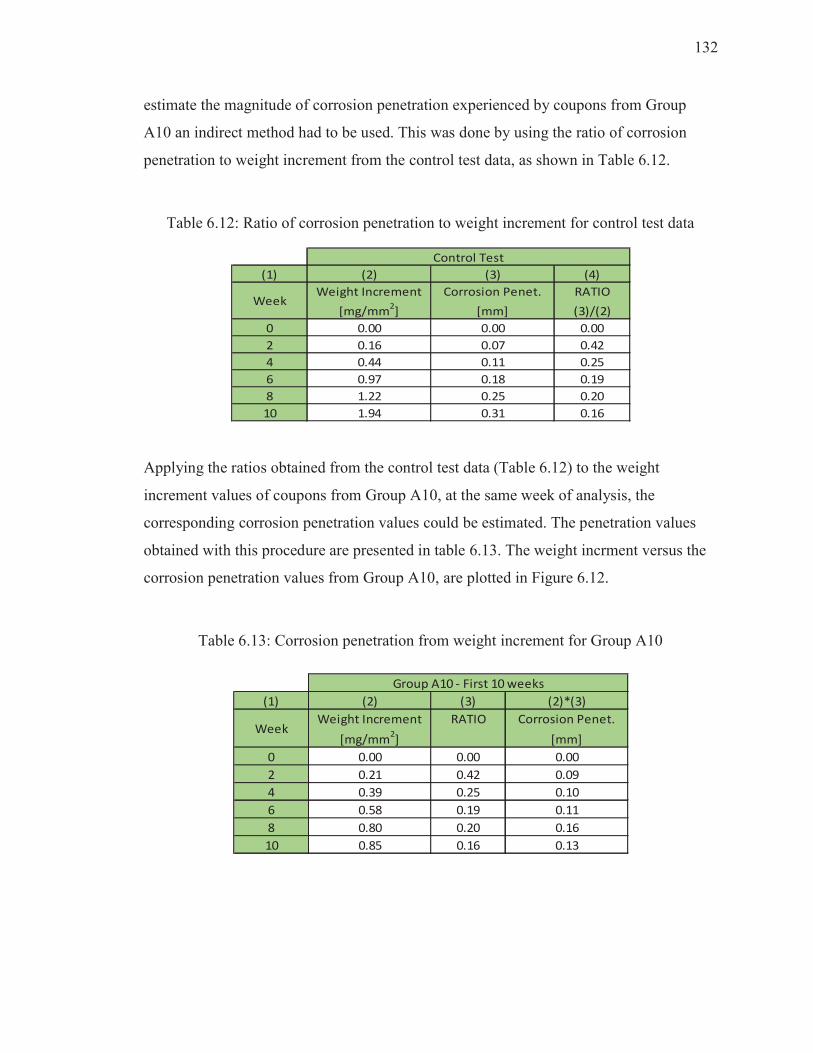
132
estimate the magnitude of corrosion penetration experienced by coupons from Group
A10 an indirect method had to be used. This was done by using the ratio of corrosion
penetration to weight increment from the control test data, as shown in Table 6.12.
Table 6.12: Ratio of corrosion penetration to weight increment for control test data
(1) (2) (3) (4)
Weight Increment Corrosion Penet. RATIO
[mg/mm2] [mm] (3)/(2)
0 0.00 0.00 0.00
2 0.16 0.07 0.42
4 0.44 0.11 0.25
6 0.97 0.18 0.19
8 1.22 0.25 0.20
10 1.94 0.31 0.16
Week
Control Test
Applying the ratios obtained from the control test data (Table 6.12) to the weight
increment values of coupons from Group A10, at the same week of analysis, the
corresponding corrosion penetration values could be estimated. The penetration values
obtained with this procedure are presented in table 6.13. The weight incrment versus the
corrosion penetration values from Group A10, are plotted in Figure 6.12.
Table 6.13: Corrosion penetration from weight increment for Group A10
(1) (2) (3) (2)*(3)
Weight Increment RATIO Corrosion Penet.
[mg/mm2] [mm]
0 0.00 0.00 0.00
2 0.21 0.42 0.09
4 0.39 0.25 0.10
6 0.58 0.19 0.11
8 0.80 0.20 0.16
10 0.85 0.16 0.13
Week
Group A10 - First 10 weeks
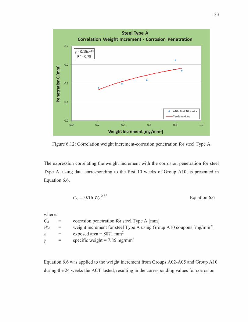
133
y = 0.15x0.38
R² = 0.79
0.0
0.1
0.1
0.2
0.2
0.0 0.2 0.4 0.6 0.8 1.0
Pe
ne
tra
tio
n C
[m
m]
Weight Increment [mg/mm2]
Steel Type A
Correlation Weight Increment - Corrosion Penetration
A10 - First 10 weeks
Tendency Line
Figure 6.12: Correlation weight increment-corrosion penetration for steel Type A
The expression correlating the weight increment with the corrosion penetration for steel
Type A, using data corresponding to the first 10 weeks of Group A10, is presented in
Equation 6.6.
�� � 0.15 ��
�.� Equation 6.6
where:
CA = corrosion penetration for steel Type A [mm]
WA = weight increment for steel Type A using Group A10 coupons [mg/mm2]
A = exposed area = 8871 mm2
γ = specific weight = 7.85 mg/mm3
Equation 6.6 was applied to the weight increment from Groups A02-A05 and Group A10
during the 24 weeks the ACT lasted, resulting in the corresponding values for corrosion
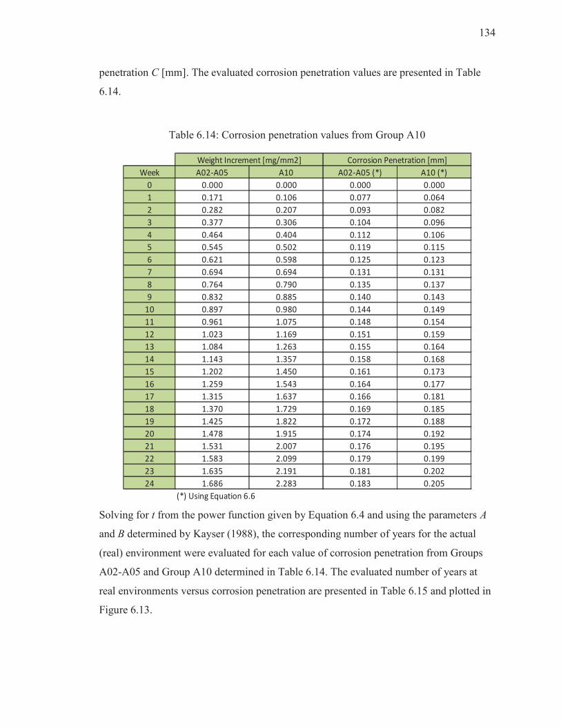
134
penetration C [mm]. The evaluated corrosion penetration values are presented in Table
6.14.
Table 6.14: Corrosion penetration values from Group A10
Week A02-A05 A10 A02-A05 (*) A10 (*)
0 0.000 0.000 0.000 0.000
1 0.171 0.106 0.077 0.064
2 0.282 0.207 0.093 0.082
3 0.377 0.306 0.104 0.096
4 0.464 0.404 0.112 0.106
5 0.545 0.502 0.119 0.115
6 0.621 0.598 0.125 0.123
7 0.694 0.694 0.131 0.131
8 0.764 0.790 0.135 0.137
9 0.832 0.885 0.140 0.143
10 0.897 0.980 0.144 0.149
11 0.961 1.075 0.148 0.154
12 1.023 1.169 0.151 0.159
13 1.084 1.263 0.155 0.164
14 1.143 1.357 0.158 0.168
15 1.202 1.450 0.161 0.173
16 1.259 1.543 0.164 0.177
17 1.315 1.637 0.166 0.181
18 1.370 1.729 0.169 0.185
19 1.425 1.822 0.172 0.188
20 1.478 1.915 0.174 0.192
21 1.531 2.007 0.176 0.195
22 1.583 2.099 0.179 0.199
23 1.635 2.191 0.181 0.202
24 1.686 2.283 0.183 0.205
(*) Using Equation 6.6
Weight Increment [mg/mm2] Corrosion Penetration [mm]
Solving for t from the power function given by Equation 6.4 and using the parameters A
and B determined by Kayser (1988), the corresponding number of years for the actual
(real) environment were evaluated for each value of corrosion penetration from Groups
A02-A05 and Group A10 determined in Table 6.14. The evaluated number of years at
real environments versus corrosion penetration are presented in Table 6.15 and plotted in
Figure 6.13.
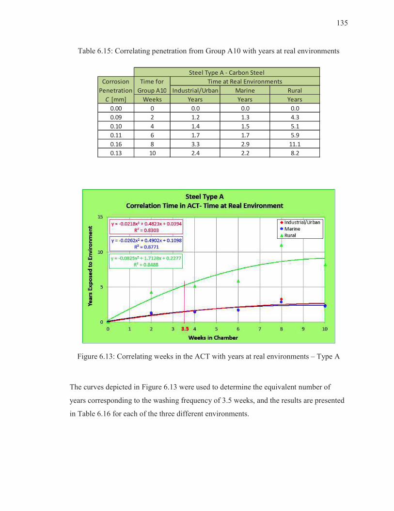
135
Table 6.15: Correlating penetration from Group A10 with years at real environments
Industrial/Urban Marine Rural
Weeks Years Years Years
0.00 0 0.0 0.0 0.0
0.09 2 1.2 1.3 4.3
0.10 4 1.4 1.5 5.1
0.11 6 1.7 1.7 5.9
0.16 8 3.3 2.9 11.1
0.13 10 2.4 2.2 8.2
Steel Type A - Carbon Steel
Corrosion
Penetration
C [mm]
Time for
Group A10
Time at Real Environments
Figure 6.13: Correlating weeks in the ACT with years at real environments – Type A
The curves depicted in Figure 6.13 were used to determine the equivalent number of
years corresponding to the washing frequency of 3.5 weeks, and the results are presented
in Table 6.16 for each of the three different environments.
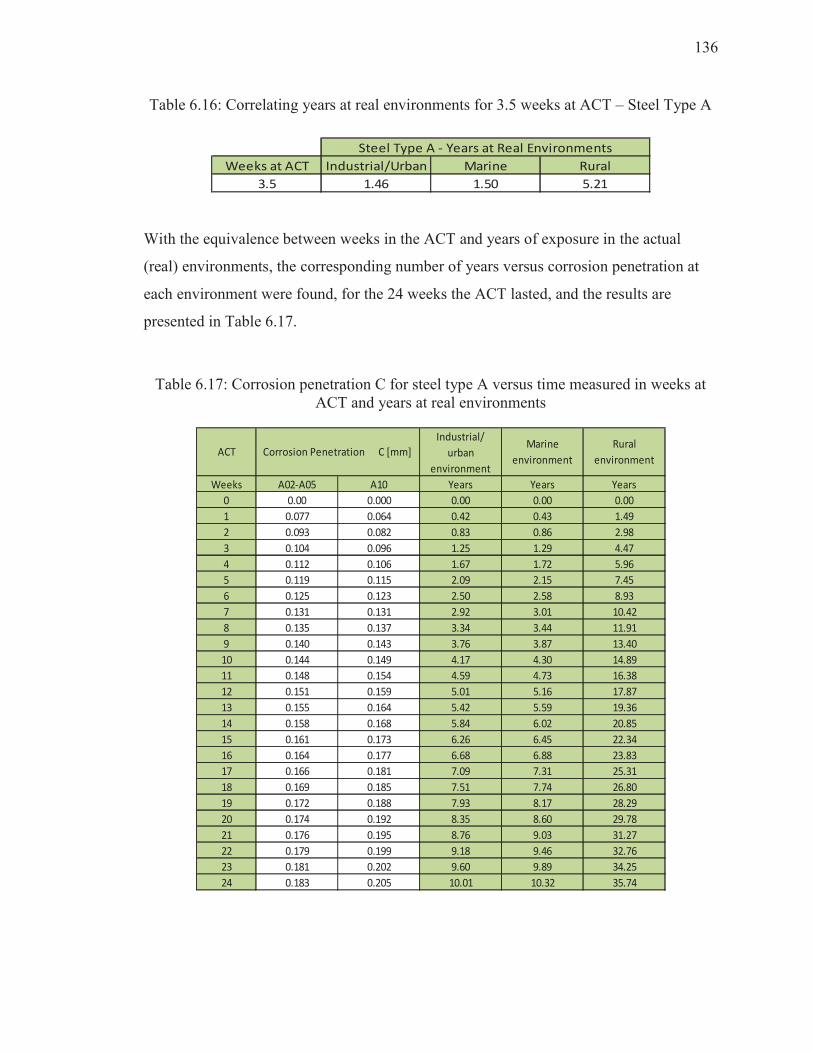
136
Table 6.16: Correlating years at real environments for 3.5 weeks at ACT – Steel Type A
Weeks at ACT Industrial/Urban Marine Rural
3.5 1.46 1.50 5.21
Steel Type A - Years at Real Environments
With the equivalence between weeks in the ACT and years of exposure in the actual
(real) environments, the corresponding number of years versus corrosion penetration at
each environment were found, for the 24 weeks the ACT lasted, and the results are
presented in Table 6.17.
Table 6.17: Corrosion penetration C for steel type A versus time measured in weeks at ACT and years at real environments
Weeks A02-A05 A10 Years Years Years
0 0.00 0.000 0.00 0.00 0.00
1 0.077 0.064 0.42 0.43 1.49
2 0.093 0.082 0.83 0.86 2.98
3 0.104 0.096 1.25 1.29 4.47
4 0.112 0.106 1.67 1.72 5.96
5 0.119 0.115 2.09 2.15 7.45
6 0.125 0.123 2.50 2.58 8.93
7 0.131 0.131 2.92 3.01 10.42
8 0.135 0.137 3.34 3.44 11.91
9 0.140 0.143 3.76 3.87 13.40
10 0.144 0.149 4.17 4.30 14.89
11 0.148 0.154 4.59 4.73 16.38
12 0.151 0.159 5.01 5.16 17.87
13 0.155 0.164 5.42 5.59 19.36
14 0.158 0.168 5.84 6.02 20.85
15 0.161 0.173 6.26 6.45 22.34
16 0.164 0.177 6.68 6.88 23.83
17 0.166 0.181 7.09 7.31 25.31
18 0.169 0.185 7.51 7.74 26.80
19 0.172 0.188 7.93 8.17 28.29
20 0.174 0.192 8.35 8.60 29.78
21 0.176 0.195 8.76 9.03 31.27
22 0.179 0.199 9.18 9.46 32.76
23 0.181 0.202 9.60 9.89 34.25
24 0.183 0.205 10.01 10.32 35.74
ACT Corrosion Penetration C [mm]
Industrial/
urban
environment
Marine
environment
Rural
environment
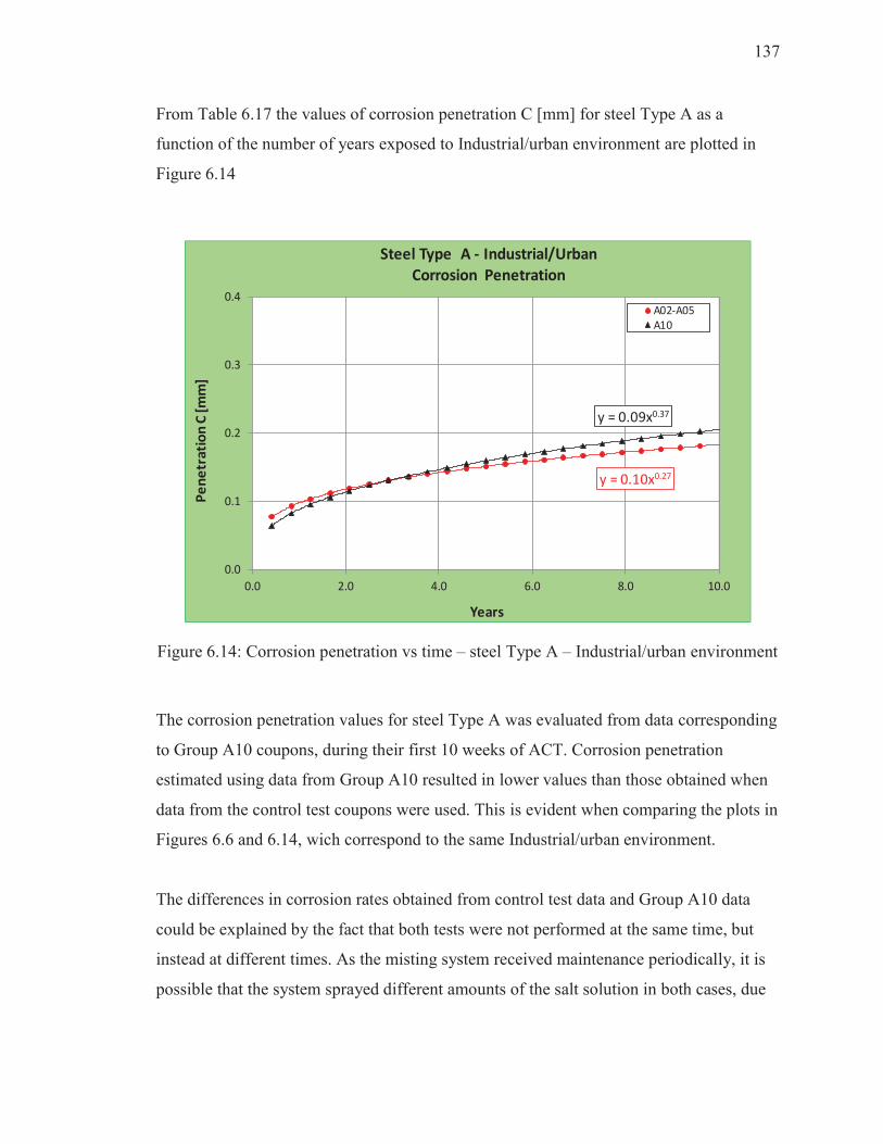
137
From Table 6.17 the values of corrosion penetration C [mm] for steel Type A as a
function of the number of years exposed to Industrial/urban environment are plotted in
Figure 6.14
y = 0.10x0.27
y = 0.09x0.37
0.0
0.1
0.2
0.3
0.4
0.0 2.0 4.0 6.0 8.0 10.0
Pe
ne
tra
tio
n C
[m
m]
Years
Steel Type A - Industrial/Urban
Corrosion Penetration
A02-A05
A10
Figure 6.14: Corrosion penetration vs time – steel Type A – Industrial/urban environment
The corrosion penetration values for steel Type A was evaluated from data corresponding
to Group A10 coupons, during their first 10 weeks of ACT. Corrosion penetration
estimated using data from Group A10 resulted in lower values than those obtained when
data from the control test coupons were used. This is evident when comparing the plots in
Figures 6.6 and 6.14, wich correspond to the same Industrial/urban environment.
The differences in corrosion rates obtained from control test data and Group A10 data
could be explained by the fact that both tests were not performed at the same time, but
instead at different times. As the misting system received maintenance periodically, it is
possible that the system sprayed different amounts of the salt solution in both cases, due
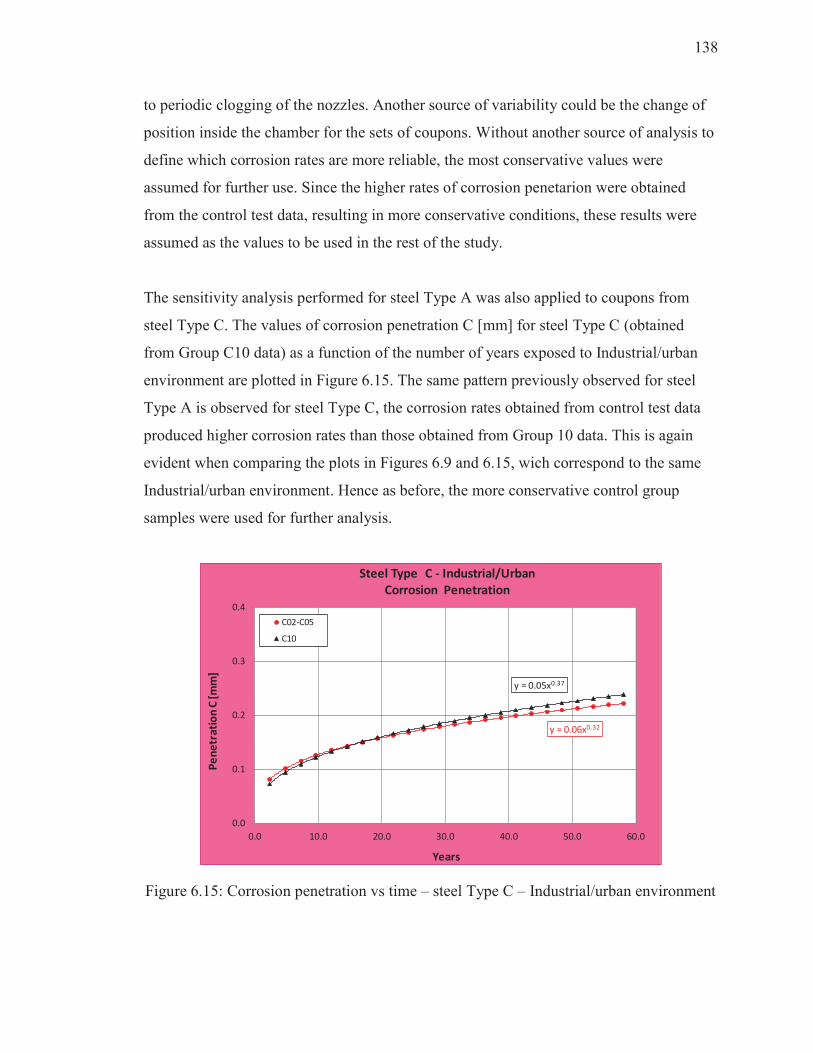
138
to periodic clogging of the nozzles. Another source of variability could be the change of
position inside the chamber for the sets of coupons. Without another source of analysis to
define which corrosion rates are more reliable, the most conservative values were
assumed for further use. Since the higher rates of corrosion penetarion were obtained
from the control test data, resulting in more conservative conditions, these results were
assumed as the values to be used in the rest of the study.
The sensitivity analysis performed for steel Type A was also applied to coupons from
steel Type C. The values of corrosion penetration C [mm] for steel Type C (obtained
from Group C10 data) as a function of the number of years exposed to Industrial/urban
environment are plotted in Figure 6.15. The same pattern previously observed for steel
Type A is observed for steel Type C, the corrosion rates obtained from control test data
produced higher corrosion rates than those obtained from Group 10 data. This is again
evident when comparing the plots in Figures 6.9 and 6.15, wich correspond to the same
Industrial/urban environment. Hence as before, the more conservative control group
samples were used for further analysis.
y = 0.06x0.32
y = 0.05x0.37
0.0
0.1
0.2
0.3
0.4
0.0 10.0 20.0 30.0 40.0 50.0 60.0
Pe
ne
tra
tio
n C
[m
m]
Years
Steel Type C - Industrial/Urban
Corrosion Penetration
C02-C05
C10
Figure 6.15: Corrosion penetration vs time – steel Type C – Industrial/urban environment
139
STRUCTURAL ANALYSIS, DESIGN, AND LOAD RATING
7.1 Introduction
The structural capacity degradation of typical steel girder highway bridges due to
atmospheric corrosion attack is presented in this chapter. The study used the deterioration
models presented in chapter 3 and corrosion penetration values obtained in chapter 6 for
different steel types and environments. The most critical corrosion rates, those obtained
from control test data, were employed since they provided the most conservative results.
Typical steel girder highway bridges were considered with variations of the span length,
number of spans, steel types, environment types, maintenance alternatives, and bridge
structure age. The emphasis was focused on the parametric analyses of several corroded
steel girder bridges under two alternatives: first, when steel bridge girder washing was
performed according to the frequency determined on chapter 6, and second, when no
bridge girder washing was performed. The reduction of structural capacity was observed
for both alternatives throughout the structure service life, which was estimated to be 100
years. The structural capacity degradation was measured through the evaluation of
moment and shear capacity for the steel girders and the measure of the corresponding
bridge load rating. The maximum elastic deflection of girders was also estimated as a
measure of the structural serviceability reduction.
The structural analysis and design, and load rating were based on the adherence to the
ASSHTO LRFD Bridge Design Specifications (AASHTO, 2012), and the AASHTO
Manual for Bridge Evaluation (AASHTO, 2011). A commercial software package was
used to conduct the structural analyses of typical highway steel girder bridges. Several
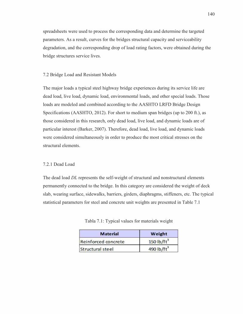
140
spreadsheets were used to process the corresponding data and determine the targeted
parameters. As a result, curves for the bridges structural capacity and serviceability
degradation, and the corresponding drop of load rating factors, were obtained during the
bridge structures service lives.
7.2 Bridge Load and Resistant Models
The major loads a typical steel highway bridge experiences during its service life are
dead load, live load, dynamic load, environmental loads, and other special loads. Those
loads are modeled and combined according to the AASHTO LRFD Bridge Design
Specifications (AASHTO, 2012). For short to medium span bridges (up to 200 ft.), as
those considered in this research, only dead load, live load, and dynamic loads are of
particular interest (Barker, 2007). Therefore, dead load, live load, and dynamic loads
were considered simultaneously in order to produce the most critical stresses on the
structural elements.
7.2.1 Dead Load
The dead load DL represents the self-weight of structural and nonstructural elements
permanently connected to the bridge. In this category are considered the weight of deck
slab, wearing surface, sidewalks, barriers, girders, diaphragms, stiffeners, etc. The typical
statistical parameters for steel and concrete unit weights are presented in Table 7.1
Tabla 7.1: Typical values for materials weight
141
7.2.2 Live Load
The live load LL represents the forces produced by moving vehicles on the bridge deck.
The live load is affected by several parameters such as: span length, truck weight, axle
loads and configuration, number of vehicles, transverse position of vehicle, traffic
volume, girder spacing, and stiffness of deck and girders (Tantawi, 1986; Czarnecki,
2006). The live load is a very uncertain variable, and it is specified by means of a
“notional” load model since they do not represent any particular truck (AASHTO, 2012).
According to the ASSHTO LRFD Bridge Design Specifications (AASHTO, 2012) the
vehicular live loading, designated as HL-93, consist of a combination of three loads: the
design truck, the design tandem, and the design lane load. The three live load
combinations proposed by the code are presented in Figure 7.1
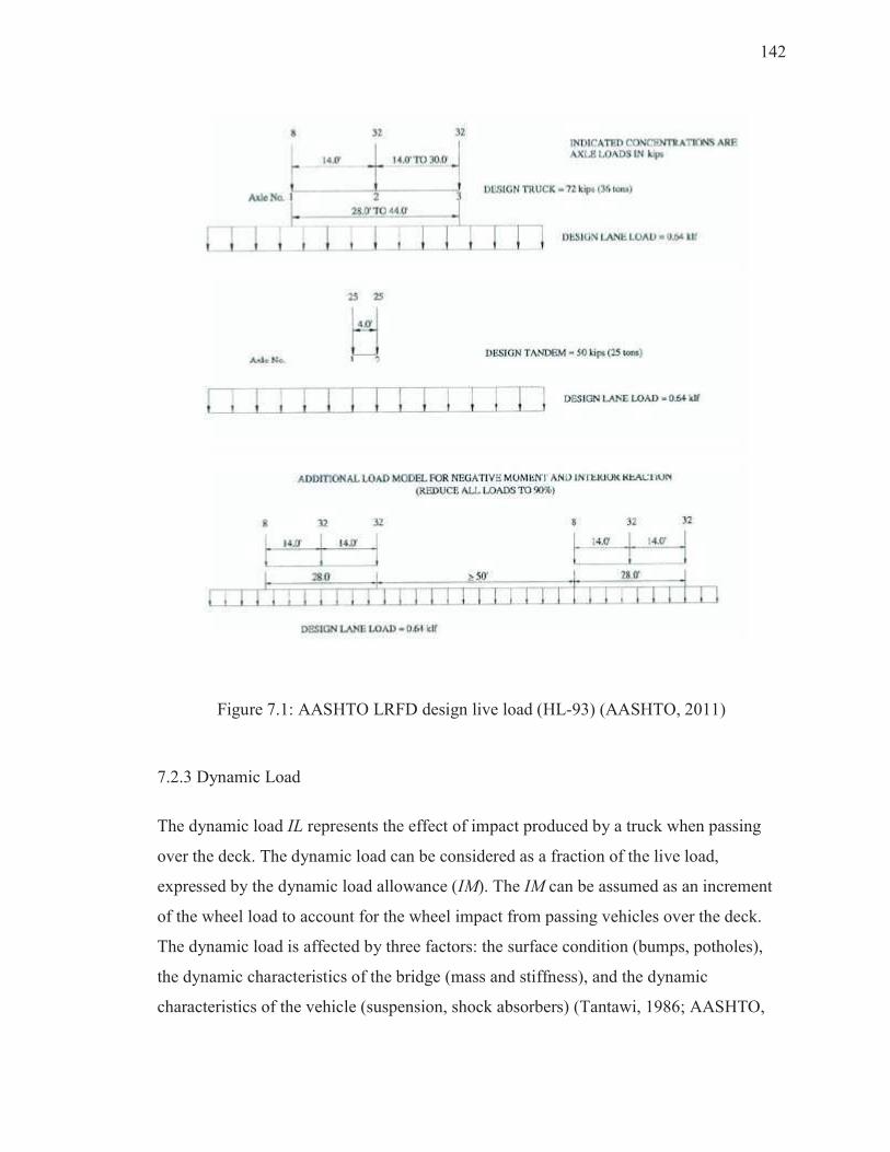
142
Figure 7.1: AASHTO LRFD design live load (HL-93) (AASHTO, 2011)
7.2.3 Dynamic Load
The dynamic load IL represents the effect of impact produced by a truck when passing
over the deck. The dynamic load can be considered as a fraction of the live load,
expressed by the dynamic load allowance (IM). The IM can be assumed as an increment
of the wheel load to account for the wheel impact from passing vehicles over the deck.
The dynamic load is affected by three factors: the surface condition (bumps, potholes),
the dynamic characteristics of the bridge (mass and stiffness), and the dynamic
characteristics of the vehicle (suspension, shock absorbers) (Tantawi, 1986; AASHTO,
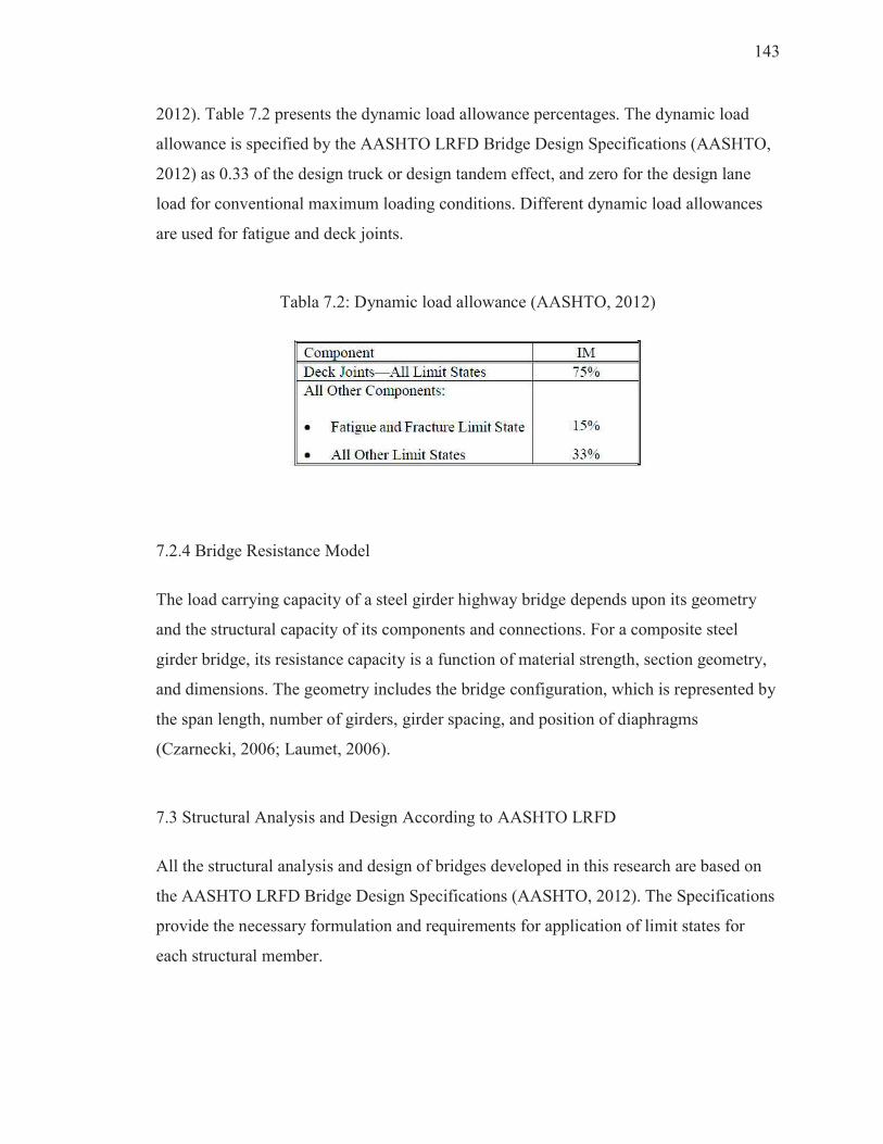
143
2012). Table 7.2 presents the dynamic load allowance percentages. The dynamic load
allowance is specified by the AASHTO LRFD Bridge Design Specifications (AASHTO,
2012) as 0.33 of the design truck or design tandem effect, and zero for the design lane
load for conventional maximum loading conditions. Different dynamic load allowances
are used for fatigue and deck joints.
Tabla 7.2: Dynamic load allowance (AASHTO, 2012)
7.2.4 Bridge Resistance Model
The load carrying capacity of a steel girder highway bridge depends upon its geometry
and the structural capacity of its components and connections. For a composite steel
girder bridge, its resistance capacity is a function of material strength, section geometry,
and dimensions. The geometry includes the bridge configuration, which is represented by
the span length, number of girders, girder spacing, and position of diaphragms
(Czarnecki, 2006; Laumet, 2006).
7.3 Structural Analysis and Design According to AASHTO LRFD
All the structural analysis and design of bridges developed in this research are based on
the AASHTO LRFD Bridge Design Specifications (AASHTO, 2012). The Specifications
provide the necessary formulation and requirements for application of limit states for
each structural member.
144
Based on the specifications given by the AASHTO LRFD code, analytical models were
created to analyze several typical steel girder highway bridges. The models included the
following factors for an appropriate analysis and design: structural capacity, load
combinations, and evaluation of maximum stresses and deformations. A parametric
structural analysis was performed, based on the typical steel bridges designed, focusing
on the progressive corrosion of steel girders. Simple supported and two-span continuous
I-girder bridges were analyzed and load rating was performed for different ages
throughout the expected bridge service life.
7.3.1 Representative I-Girder Steel Bridges Considered
Most bridges can be divided into two main parts: superstructure and substructure. The
substructure supports the superstructure and transfers loads to the foundation. The
superstructure, on the other hand, is the part of the bridge which provides support for the
traffic. The superstructure of a steel girder bridge is composed of the deck, girders,
diaphragms, and stiffeners as structural elements. Also the superstructure could include
some nonstructural elements such as wearing surface, barriers, sidewalks, stay-in-place
forms, signs, etc. In this research typical steel girder superstructures were considered for
analysis and design. The analysis and design of the substructure was not considered
herein, since the parametric analysis of corroded girders does not affect substantially
these parts of a bridge. Consequently, only code expressions and requirements related to
the superstructure analysis and design are presented in this chapter.
To appreciate the structural capacity degradation of steel girder bridges due to
atmospheric corrosion, typical highway bridge configurations were considered. A typical
bridge section was assumed to be similar to that described in the document “AASHTO
Steel Bridge Design Handbook Vol. 21- Design Example 2A: Two-Span Continuous
Straight Composite Steel I-Girder Bridge” (Barth, 2012). Figure 7.2 shows the typical
cross section for the steel girder bridges considered. The section is considered as a
representative of steel highway bridges in the USA, wide enough for two lanes.
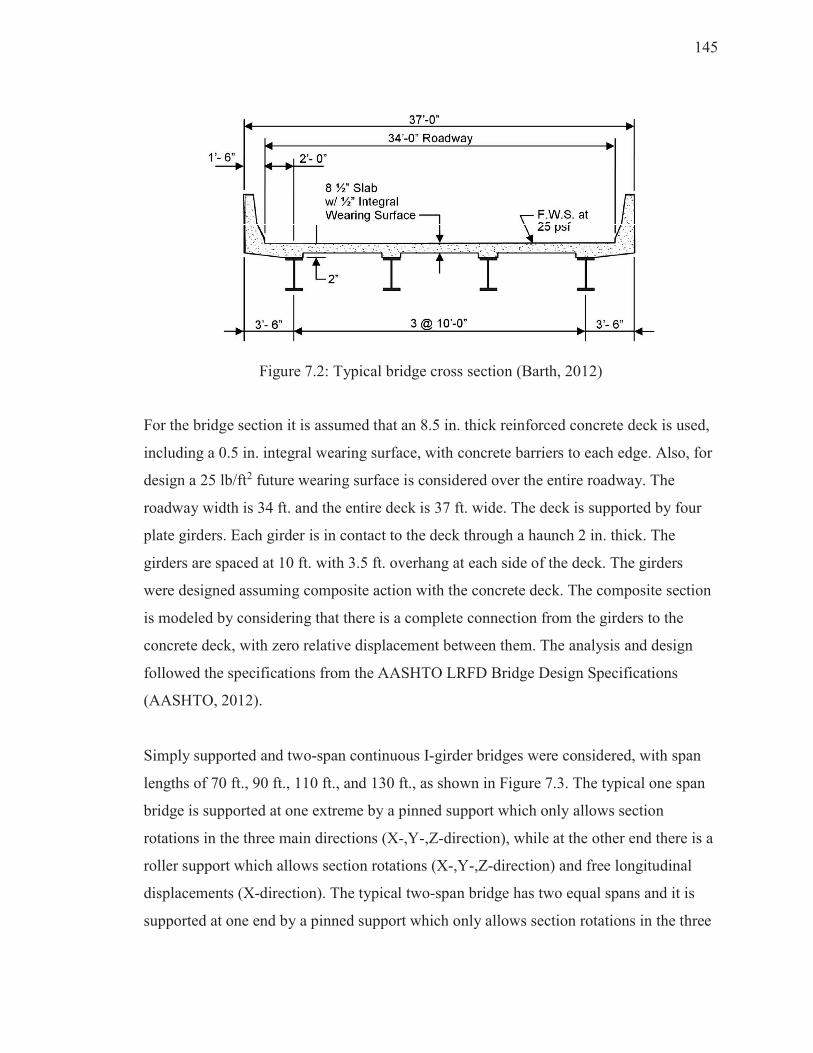
145
Figure 7.2: Typical bridge cross section (Barth, 2012)
For the bridge section it is assumed that an 8.5 in. thick reinforced concrete deck is used,
including a 0.5 in. integral wearing surface, with concrete barriers to each edge. Also, for
design a 25 lb/ft2 future wearing surface is considered over the entire roadway. The
roadway width is 34 ft. and the entire deck is 37 ft. wide. The deck is supported by four
plate girders. Each girder is in contact to the deck through a haunch 2 in. thick. The
girders are spaced at 10 ft. with 3.5 ft. overhang at each side of the deck. The girders
were designed assuming composite action with the concrete deck. The composite section
is modeled by considering that there is a complete connection from the girders to the
concrete deck, with zero relative displacement between them. The analysis and design
followed the specifications from the AASHTO LRFD Bridge Design Specifications
(AASHTO, 2012).
Simply supported and two-span continuous I-girder bridges were considered, with span
lengths of 70 ft., 90 ft., 110 ft., and 130 ft., as shown in Figure 7.3. The typical one span
bridge is supported at one extreme by a pinned support which only allows section
rotations in the three main directions (X-,Y-,Z-direction), while at the other end there is a
roller support which allows section rotations (X-,Y-,Z-direction) and free longitudinal
displacements (X-direction). The typical two-span bridge has two equal spans and it is
supported at one end by a pinned support which only allows section rotations in the three

146
main directions (X-,Y-,Z-direction), while at the bent and in the other end there are roller
supports which allow section rotations (X-,Y-,Z-direction) and free longitudinal
displacements (X-direction).

147
Fig
ure
7.3
: S
ket
ch o
f lo
ngit
ud
inal
vie
w f
or
typ
ical
on
e-sp
an a
nd
tw
o-s
pan
bri
dges
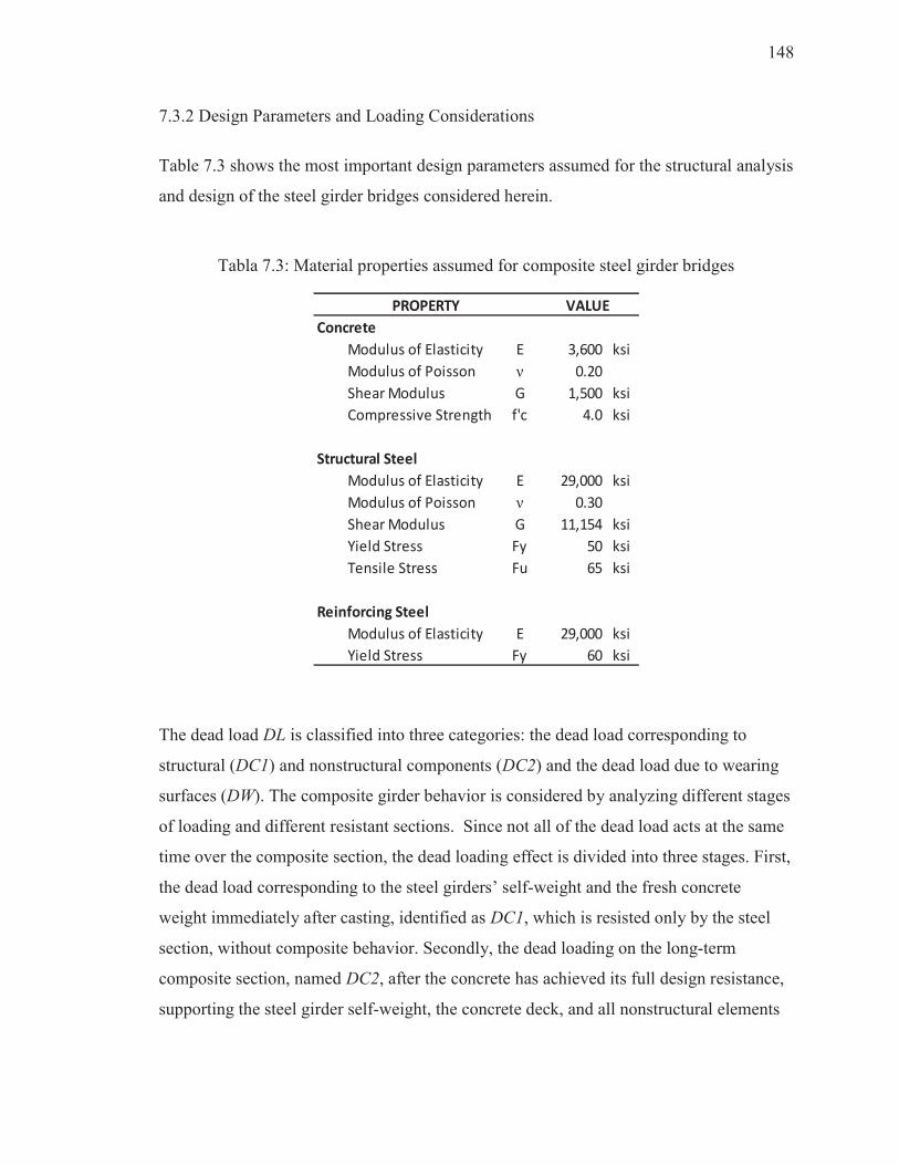
148
7.3.2 Design Parameters and Loading Considerations
Table 7.3 shows the most important design parameters assumed for the structural analysis
and design of the steel girder bridges considered herein.
Tabla 7.3: Material properties assumed for composite steel girder bridges
Concrete
Modulus of Elasticity E 3,600 ksi
Modulus of Poisson ν 0.20
Shear Modulus G 1,500 ksi
Compressive Strength f'c 4.0 ksi
Structural Steel
Modulus of Elasticity E 29,000 ksi
Modulus of Poisson ν 0.30
Shear Modulus G 11,154 ksi
Yield Stress Fy 50 ksi
Tensile Stress Fu 65 ksi
Reinforcing Steel
Modulus of Elasticity E 29,000 ksi
Yield Stress Fy 60 ksi
PROPERTY VALUE
The dead load DL is classified into three categories: the dead load corresponding to
structural (DC1) and nonstructural components (DC2) and the dead load due to wearing
surfaces (DW). The composite girder behavior is considered by analyzing different stages
of loading and different resistant sections. Since not all of the dead load acts at the same
time over the composite section, the dead loading effect is divided into three stages. First,
the dead load corresponding to the steel girders’ self-weight and the fresh concrete
weight immediately after casting, identified as DC1, which is resisted only by the steel
section, without composite behavior. Secondly, the dead loading on the long-term
composite section, named DC2, after the concrete has achieved its full design resistance,
supporting the steel girder self-weight, the concrete deck, and all nonstructural elements
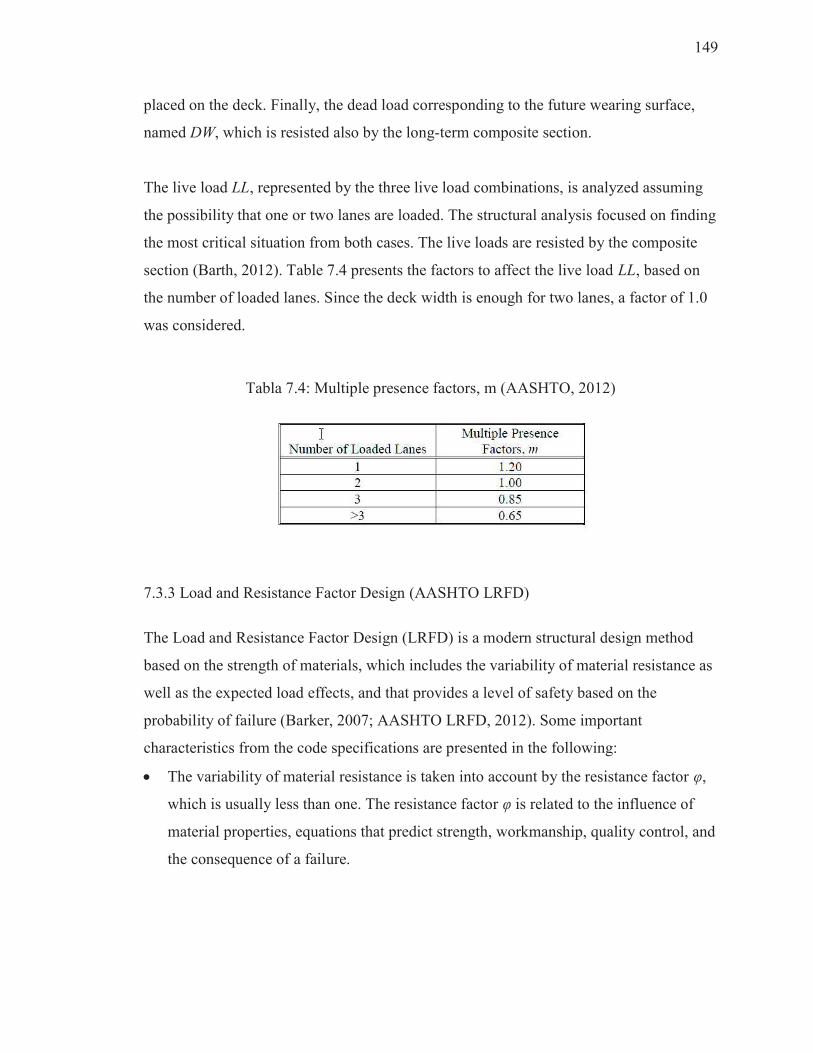
149
placed on the deck. Finally, the dead load corresponding to the future wearing surface,
named DW, which is resisted also by the long-term composite section.
The live load LL, represented by the three live load combinations, is analyzed assuming
the possibility that one or two lanes are loaded. The structural analysis focused on finding
the most critical situation from both cases. The live loads are resisted by the composite
section (Barth, 2012). Table 7.4 presents the factors to affect the live load LL, based on
the number of loaded lanes. Since the deck width is enough for two lanes, a factor of 1.0
was considered.
Tabla 7.4: Multiple presence factors, m (AASHTO, 2012)
7.3.3 Load and Resistance Factor Design (AASHTO LRFD)
The Load and Resistance Factor Design (LRFD) is a modern structural design method
based on the strength of materials, which includes the variability of material resistance as
well as the expected load effects, and that provides a level of safety based on the
probability of failure (Barker, 2007; AASHTO LRFD, 2012). Some important
characteristics from the code specifications are presented in the following:
· The variability of material resistance is taken into account by the resistance factor φ,
which is usually less than one. The resistance factor φ is related to the influence of
material properties, equations that predict strength, workmanship, quality control, and
the consequence of a failure.
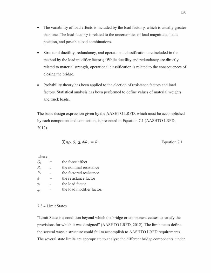
150
· The variability of load effects is included by the load factor γ, which is usually greater
than one. The load factor γ is related to the uncertainties of load magnitude, loads
position, and possible load combinations.
· Structural ductility, redundancy, and operational classification are included in the
method by the load modifier factor η. While ductility and redundancy are directly
related to material strength, operational classification is related to the consequences of
closing the bridge.
· Probability theory has been applied to the election of resistance factors and load
factors. Statistical analysis has been performed to define values of material weights
and truck loads.
The basic design expression given by the AASHTO LRFD, which must be accomplished
by each component and connection, is presented in Equation 7.1 (AASHTO LRFD,
2012).
∑������ � �� ! �" Equation 7.1
where:
Qi = the force effect
Rn = the nominal resistance
Rr = the factored resistance
ϕ = the resistance factor
γi = the load factor
ηi = the load modifier factor.
7.3.4 Limit States
“Limit State is a condition beyond which the bridge or component ceases to satisfy the
provisions for which it was designed” (AASHTO LRFD, 2012). The limit states define
the several ways a structure could fail to accomplish to AASHTO LRFD requirements.
The several state limits are appropriate to analyze the different bridge components, under
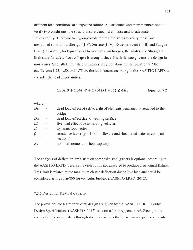
151
different load conditions and expected failure. All structures and their members should
verify two conditions: the structural safety against collapse and its adequate
serviceability. There are four groups of different limit states to verify those two
mentioned conditions: Strength (I-V), Service (I-IV), Extreme Event (I - II) and Fatigue
(I – II). However, for typical short to medium span bridges, the analysis of Strength I
limit state for safety from collapse is enough, since this limit state governs the design in
most cases. Strength I limit state is expressed by Equation 7.2. In Equation 7.2 the
coefficients 1.25, 1.50, and 1.75 are the load factors according to the AASHTO LRFD, to
consider the load uncertainties.
1.25�� � 1.50�� � 1.75���1 � �� ! "#$ Equation 7.2
where:
DD = dead load effect of self-weight of elements permanently attached to the
bridge
DW = dead load effect due to wearing surface
LL = live load effect due to moving vehicles
IL = dynamic load factor
ϕ = resistance factor (ϕ = 1.00 for flexure and shear limit states in compact
sections)
Rn = nominal moment or shear capacity
The analysis of deflection limit state on composite steel girders is optional according to
the AASHTO LRFD, because its violation is not expected to produce a structural failure.
This limit is related to the maximum elastic deflection due to live load and could be
considered as the span/800 for vehicular bridges (AASHTO LRFD, 2012).
7.3.5 Design for Flexural Capacity
The provisions for I-girder flexural design are given by the AASHTO LRFD Bridge
Design Specifications (AASHTO, 2012), section 6.10 or Appendix A6. Steel girders
connected to concrete deck through shear connectors that prove an adequate composite
152
behavior should be designed according to the provisions of AASHTO LRFD Article
6.10.10. The elastic stresses at any location on the composite section should be evaluated
as the sum of three stresses caused by loads acting separately on these three different
sections: 1) steel girder section, 2) short-term composite section, and 3) long-term
composite section.
The flexural stresses for sections under positive flexure are evaluated based on a
composite section that includes the steel section and the transformed area of the effective
width of concrete deck. Concrete in tension is not considered effective in the resistant
capacity – AASHTO LRFD Article 6.10.1.1.1b. The flexural stresses for sections under
negative flexure are evaluated based on a composite section, for both short-term and
long-term moments, that includes the steel section and the longitudinal reinforcement
within the effective width of concrete deck – AASHTO LRFD Article 6.10.1.1.1c.
For a simply supported bridge, the desirable type of bending failure at ultimate capacity
is steel yielding at midspan, where the maximum positive moment occurs. This is a type
of ductile failure with pronounced deformations that provide forewarning of any
impending failure. In composite I-girder sections, a ductile failure is produced when the
structural steel starts to yield, before the concrete from the deck begins to crush. Also it is
assumed that slippage of shear connectors is not possible, assuring a perfect composite
action. Additionally, for a two-span continuous composite bridge it is possible to fail due
to buckling of its lower flange at sections in regions of negative moment near the pier
support. The slenderness of the bottom flange should be adequate to avoid this type of
undesirable failure.
The flexural design procedure for composite I-girders is not presented in this research.
Section 6.10 and Appendix A6 of the AASHTO LRFD provides all necessary
information for a complete design. Also, adequate examples of flexural design for
composite I-girders are available in the works from Czarnecki (2006), Barth (2012), and
Barker and Puckett (2007).
153
7.3.6 Design for Shear Capacity
The design of a typical composite steel girder highway bridge included verification of
adequate shear capacity. The I-girder nominal shear capacity was evaluated and
compared with the acting shear stresses from the Strength I limit state. The critical
sections for shear stresses occur near the supports at the abutments for one-span bridges,
and at the pier for two-span bridges. The shear design considered always compact
sections and it was assumed that the entire shear capacity was provided by the I-girder
web. The nominal shear resistance according to AASHTO LRFD (AASHTO, 2012) is
presented in equations 7.3 to 7.5.
�� � ���� Equation 7.3
where:
øv = resistance factor for shear
Vn = nominal shear resistance [kip]
Vu = shear at the web section under consideration due to factored loads [kip]
The nominal shear resistance of unstiffened webs shall be taken as:
�� � � ! � "�# Equation 7.4
in which:
�# � 0.58$%&'(& Equation 7.5
where:
C = ratio of the shear-buckling resistance to the shear yield strength
Vcr = shear-buckling resistance [kip]
Vn = nominal shear resistance [kip]
Vp = plastic shear force [kip]
Fyw = specified minimum yield strength of a web [kip]
154
D = web depth [in.]
tw = web thickness [in.]
The shear carrying capacity was checked during all design process, but actually it did not
govern, since flexural requirements were more critical.
7.3.7 Elastic Deflections
According to AASHTO LRFD (AASHTO, 2012) bridges should be designed with the
expressed condition “to avoid undesirable structural or psychological effects due to their
deformations (AASHTO, 2012).” The code specifies the evaluation of elastic deflections
based on the live load portion from Service I limit state, including the dynamic load
allowance effects. Although the Specifications indicates that deflection limit state is an
optional requirement related to serviceability, when applied, the deflection is limited to
1/800 of the span length for steel girders from vehicular bridges. The span length to
estimate the elastic deflection should be the free distance between centers of support
(INDOT, 2013). The estimated elastic deflection should be taken as the larger value
resulting from the application of:
• the design truck alone, or
• 25 percent of the design truck taken together with the design lane load.
The elastic deflection on composite steel I-girder bridges is affected by bridge
configuration, superstructure details, loading cases, and boundary conditions. Therefore,
a reliable estimation of elastic deformation should be achieved when all these factors are
included in the structural analysis.
7.3.8 Steel Highway Bridge Design using a FE Package
Steel I-girder bridges are the most common and effective solution for short to medium
span bridges (Caltrans, 2015). The superstructure design according to AASHTO LRFD
155
(AASHTO, 2012) requires accomplishing several relationships from the bridge geometry,
girder geometry, deck and girder materials, loading systems, etc. The procedure requires
the assumption of specific values for member dimensions, bridge elements disposition,
and material properties. Therefore, the analysis and design of one steel girder bridge is
time consuming when all requirements are checked properly. For a wide variety of steel
highway bridges, eight typical models were identified to be analyzed in this research.
One and two-span, 70, 90, 110 and 130 feet span-length bridges were selected to be
analyzed under the corrosion model identified in this study.
As an alternative to time consuming hand calculations, the use of commercial software
packages has proven to be accurate, convenient, and extremely fast in verifying all code
requirements. This approach allows to the designer to perform several run analyses for
the same bridge model, while searching for the most effective bridge configuration and
appropriate member dimensions. CSiBridge (Computers & Structures, Inc., 2011) is a
versatile, integrated, and powerful tool for the analysis and design of steel girder bridges,
developed by the same creators of SAP2000 - Computers & Structures, Inc. The package
uses the finite element method to model the bridge elements and solve the several stress-
strain relationships established for the model. The steel girder bridge analysis and design
using CSiBridge is based on the application of load patterns, load cases, load
combinations, and design requests, according to the desired code (Computers &
Structures, Inc., 2011).
To verify the suitability of using the CSiBridge package for analyzing and designing a
steel girder bridge, a comparative analysis was performed between the use of CSiBridge
and the results from a hand solution. A step by step, hand solution, was selected from the
document “AASHTO Steel Bridge Design Handbook Vol. 21- Design Example 2A:
Two-Span Continuous Straight Composite Steel I-Girder Bridge” (Barth, 2012). This is
an official document from AASHTO, where a detailed solution for a typical two-span (90
ft. – 90 ft.) continuous steel girder bridge is analyzed and designed according to the
AASHTO LRFD code. The bridge section is composed of four plate girders spaced at
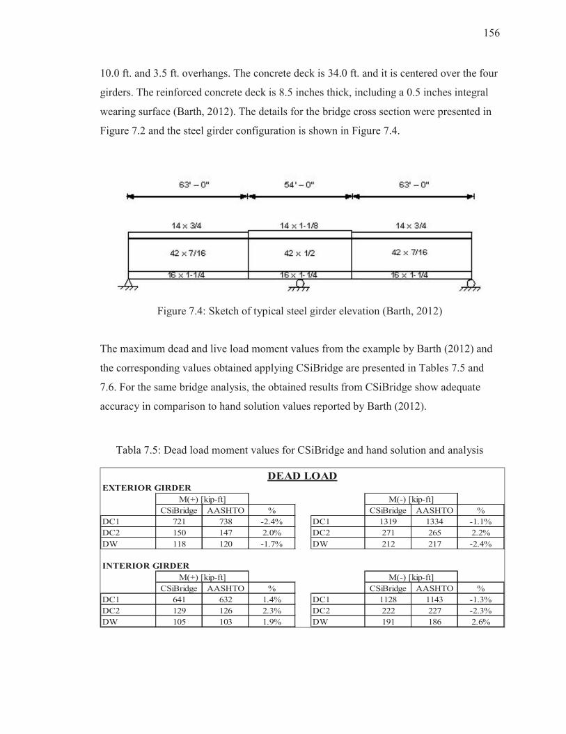
156
10.0 ft. and 3.5 ft. overhangs. The concrete deck is 34.0 ft. and it is centered over the four
girders. The reinforced concrete deck is 8.5 inches thick, including a 0.5 inches integral
wearing surface (Barth, 2012). The details for the bridge cross section were presented in
Figure 7.2 and the steel girder configuration is shown in Figure 7.4.
Figure 7.4: Sketch of typical steel girder elevation (Barth, 2012)
The maximum dead and live load moment values from the example by Barth (2012) and
the corresponding values obtained applying CSiBridge are presented in Tables 7.5 and
7.6. For the same bridge analysis, the obtained results from CSiBridge show adequate
accuracy in comparison to hand solution values reported by Barth (2012).
Tabla 7.5: Dead load moment values for CSiBridge and hand solution and analysis
EXTERIOR GIRDER
CSiBridge AASHTO % CSiBridge AASHTO %
DC1 721 738 -2.4% DC1 1319 1334 -1.1%
DC2 150 147 2.0% DC2 271 265 2.2%
DW 118 120 -1.7% DW 212 217 -2.4%
INTERIOR GIRDER
CSiBridge AASHTO % CSiBridge AASHTO %
DC1 641 632 1.4% DC1 1128 1143 -1.3%
DC2 129 126 2.3% DC2 222 227 -2.3%
DW 105 103 1.9% DW 191 186 2.6%
DEAD LOAD
M(+) [kip-ft] M(-) [kip-ft]
M(+) [kip-ft] M(-) [kip-ft]
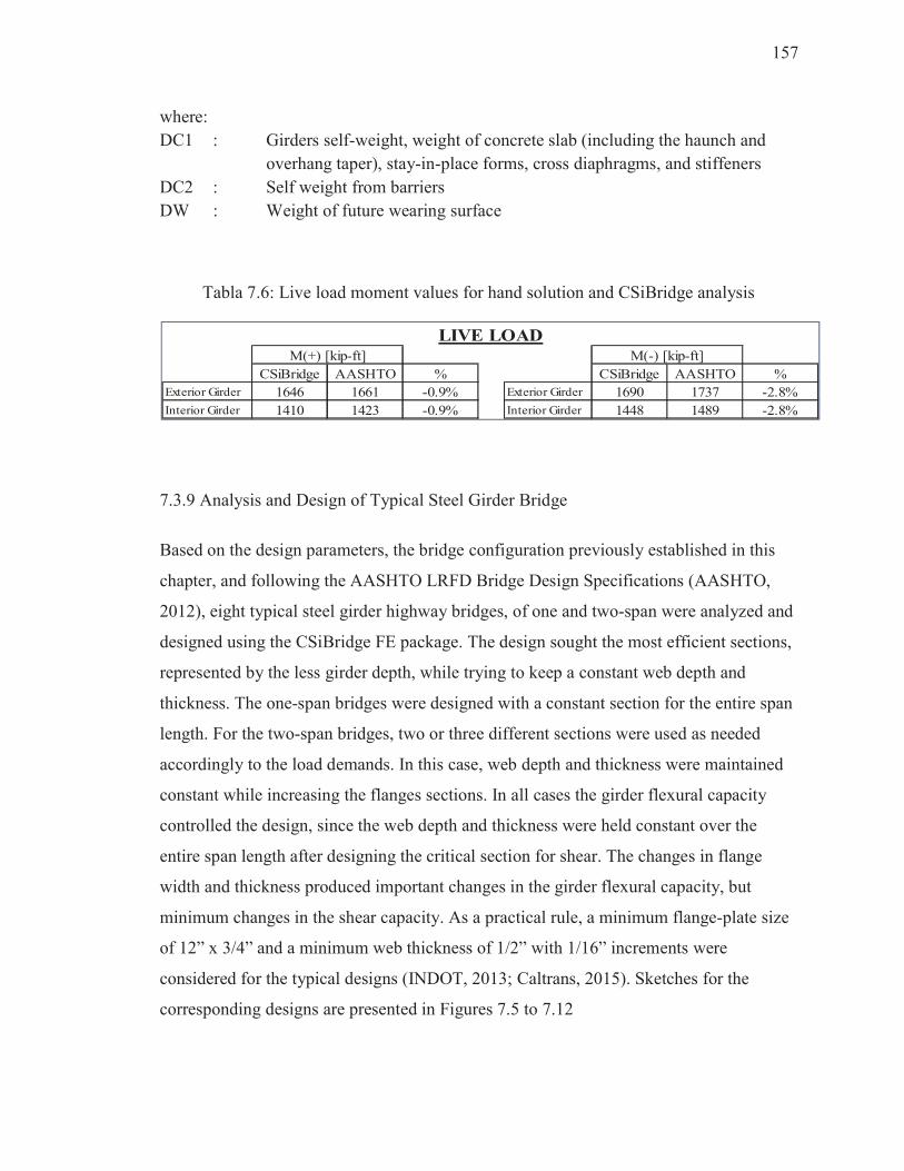
157
where:
DC1 : Girders self-weight, weight of concrete slab (including the haunch and
overhang taper), stay-in-place forms, cross diaphragms, and stiffeners
DC2 : Self weight from barriers
DW : Weight of future wearing surface
Tabla 7.6: Live load moment values for hand solution and CSiBridge analysis
7.3.9 Analysis and Design of Typical Steel Girder Bridge
Based on the design parameters, the bridge configuration previously established in this
chapter, and following the AASHTO LRFD Bridge Design Specifications (AASHTO,
2012), eight typical steel girder highway bridges, of one and two-span were analyzed and
designed using the CSiBridge FE package. The design sought the most efficient sections,
represented by the less girder depth, while trying to keep a constant web depth and
thickness. The one-span bridges were designed with a constant section for the entire span
length. For the two-span bridges, two or three different sections were used as needed
accordingly to the load demands. In this case, web depth and thickness were maintained
constant while increasing the flanges sections. In all cases the girder flexural capacity
controlled the design, since the web depth and thickness were held constant over the
entire span length after designing the critical section for shear. The changes in flange
width and thickness produced important changes in the girder flexural capacity, but
minimum changes in the shear capacity. As a practical rule, a minimum flange-plate size
of 12” x 3/4” and a minimum web thickness of 1/2” with 1/16” increments were
considered for the typical designs (INDOT, 2013; Caltrans, 2015). Sketches for the
corresponding designs are presented in Figures 7.5 to 7.12
CSiBridge AASHTO % CSiBridge AASHTO %
Exterior Girder 1646 1661 -0.9% Exterior Girder 1690 1737 -2.8%
Interior Girder 1410 1423 -0.9% Interior Girder 1448 1489 -2.8%
LIVE LOADM(+) [kip-ft] M(-) [kip-ft]
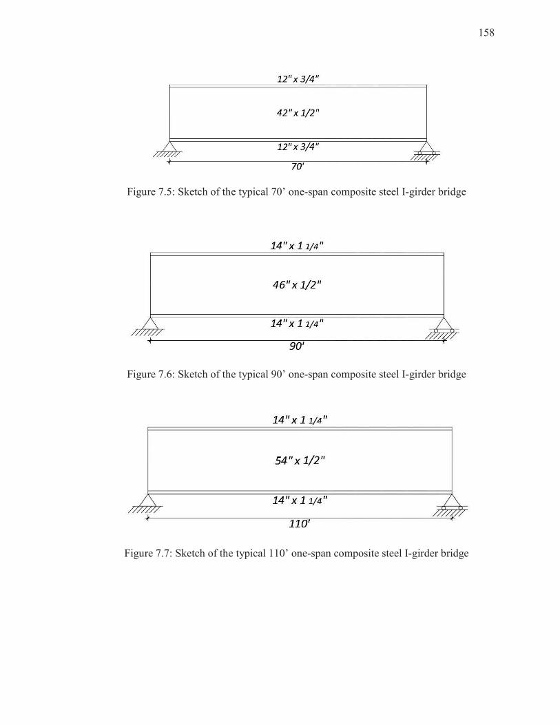
158
Figure 7.5: Sketch of the typical 70’ one-span composite steel I-girder bridge
Figure 7.6: Sketch of the typical 90’ one-span composite steel I-girder bridge
Figure 7.7: Sketch of the typical 110’ one-span composite steel I-girder bridge
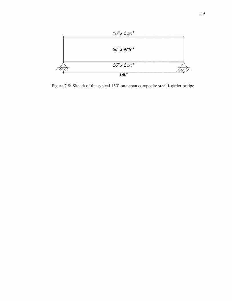
159
Figure 7.8: Sketch of the typical 130’ one-span composite steel I-girder bridge
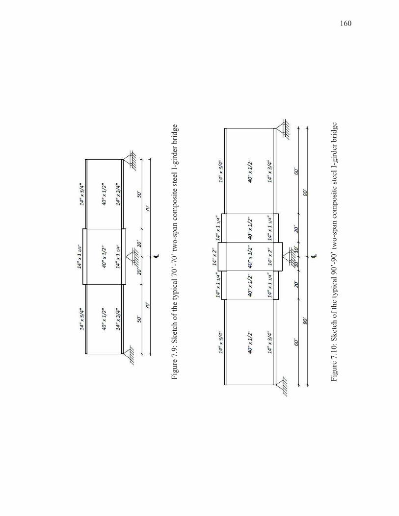
160
Fig
ure
7.9
: S
ket
ch o
f th
e ty
pic
al 7
0’-
70
’ tw
o-s
pan
co
mp
osi
te s
teel
I-g
irder
bri
dge
Fig
ure
7.1
0:
Sk
etch
of
the
typ
ical
90
’-90
’ tw
o-s
pan
com
po
site
ste
el I
-gir
der
bri
dg
e

161
Fig
ure
7.1
1:
Sk
etch
of
the
typ
ical
11
0’-
11
0’
two
-sp
an c
om
po
site
ste
el I
-gir
der
bri
dge
Fig
ure
7.1
2:
Sk
etch
of
the
typ
ical
13
0’-
13
0’
two
-sp
an c
om
po
site
ste
el I
-gir
der
bri
dge
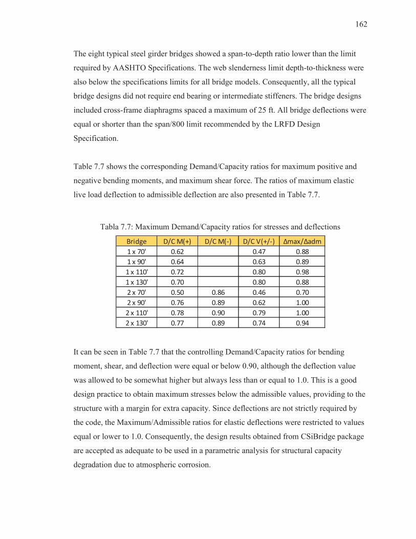
162
The eight typical steel girder bridges showed a span-to-depth ratio lower than the limit
required by AASHTO Specifications. The web slenderness limit depth-to-thickness were
also below the specifications limits for all bridge models. Consequently, all the typical
bridge designs did not require end bearing or intermediate stiffeners. The bridge designs
included cross-frame diaphragms spaced a maximum of 25 ft. All bridge deflections were
equal or shorter than the span/800 limit recommended by the LRFD Design
Specification.
Table 7.7 shows the corresponding Demand/Capacity ratios for maximum positive and
negative bending moments, and maximum shear force. The ratios of maximum elastic
live load deflection to admissible deflection are also presented in Table 7.7.
Tabla 7.7: Maximum Demand/Capacity ratios for stresses and deflections
It can be seen in Table 7.7 that the controlling Demand/Capacity ratios for bending
moment, shear, and deflection were equal or below 0.90, although the deflection value
was allowed to be somewhat higher but always less than or equal to 1.0. This is a good
design practice to obtain maximum stresses below the admissible values, providing to the
structure with a margin for extra capacity. Since deflections are not strictly required by
the code, the Maximum/Admissible ratios for elastic deflections were restricted to values
equal or lower to 1.0. Consequently, the design results obtained from CSiBridge package
are accepted as adequate to be used in a parametric analysis for structural capacity
degradation due to atmospheric corrosion.
Bridge D/C M(+) D/C M(-) D/C V(+/-) Δmax/Δadm
1 x 70' 0.62 0.47 0.88
1 x 90' 0.64 0.63 0.89
1 x 110' 0.72 0.80 0.98
1 x 130' 0.70 0.80 0.88
2 x 70' 0.50 0.86 0.46 0.70
2 x 90' 0.76 0.89 0.62 1.00
2 x 110' 0.78 0.90 0.79 1.00
2 x 130' 0.77 0.89 0.74 0.94
163
7.4 Steel Bridge Load Rating According to AASHTO MBE
Bridge load rating analysis is performed to determine the safe live load capacity of a
bridge under the conditions presented at the moment of rating. Load rating is a procedure
to estimate the actual capacity of the bridge for safety considerations. As a federal
requirement all states should perform load rating of their bridge inventory. The AASHTO
Manual for Bridge Evaluation (MBE) (AASHTO, 2011) is the official document
published by the AASHTO for current specifications on bridge load rating. According to
the AASHTO MBE, bridges should be rated for design loads and legal loads. The design
load rating is performed to be reported to the National Bridge Inventory (NBI). The legal
load rating indicates whether a bridge should be posted or strengthened (AASHTO,
2011). Bridges are posted when the structural capacity has decreased beyond the
prescribed limits.
The bridge structural capacity can decrease as the result of many factors, such as collision
damage, corrosion, modification of the section, or additional dead load. When the section
capacity decrease is due to atmospheric corrosion attack, the corrosion penetration
reduces the section thicknesses, and hence reduces the bridge structural capacity. As a
means to estimate the actual reduction of a bridge structural capacity, a load rating
analysis was performed for a series of steel girder bridges. A parametric analysis of load
rating for a series of steel girder bridges, varying some selected parameters, was
performed in order to appreciate the influence of steel washing as an effective bridge
maintenance activity. In this section are presented the details for the bridge load rating
procedure on the selected bridges.
7.4.1 Load and Resistance Factor Rating (LRFR)
The Load and Resistance Factor Rating (LRFR) is a methodology developed to provide
uniform reliability in bridge load ratings, load postings, and permit decisions (AASHTO,
2011). There are different live load models and evaluation criteria that can be used when
evaluating a bridge condition by load rating. The live load models are comprised by the
164
design live load, legal loads, and permit loads. A bridge load rating can be performed for
different purposes. Bridge load rating are required to provide information to the National
Bridge Inventory (NBI), to estimate the safety live load a bridge resists, or supporting a
bridge rehabilitation decision. The load rating methodology is constituted by three
different procedures which have to be done in a sequential manner: 1) design load rating,
2) legal load rating, and 3) permit load rating.
Load rating is an engineering process to determine the live load capacity of a bridge. This
capacity is expressed by a rating factor (RF), which is the ratio of a vehicular live load
effect (moment or shear), when the bridge is under certain limit state, to the
corresponding nominal bridge capacity. The load rating analysis offers an evaluation of
the adequacy or inadequacy of a structural element to support the load (stresses)
produced by the passage of a particular truck load. A rating factor greater than 1.0
indicates the element/structure is capable of supporting the stresses produced by the
considered live load; otherwise it fails and some actions are required. For moment and
shear capacity the most relevant analysis is the Strength I limit state. Therefore, the load
rating analysis is performed on bridges considering this limit state, and the results are the
rating factor for moment capacity (RFm) and for shear capacity (RFv). A detailed flow
chart is provided by AASHTO (2012), showing the different steps followed when
performing a bridge load rating, as it is presented in Figure 7.13.
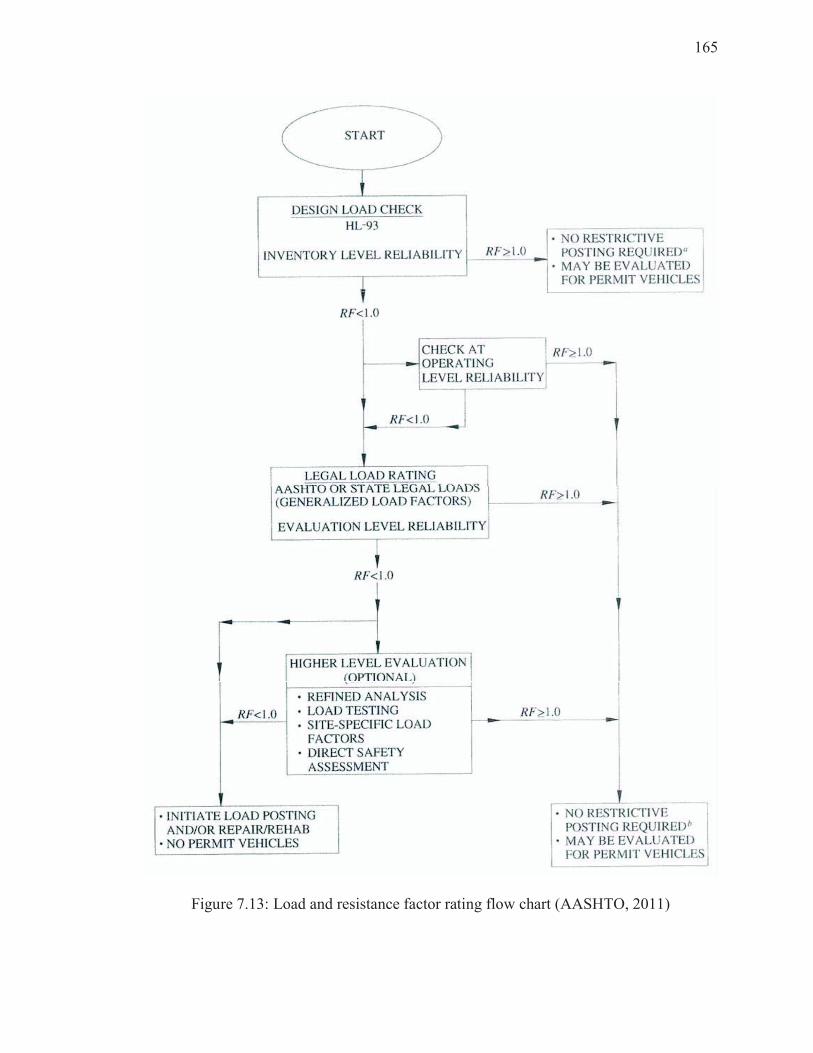
165
Figure 7.13: Load and resistance factor rating flow chart (AASHTO, 2011)
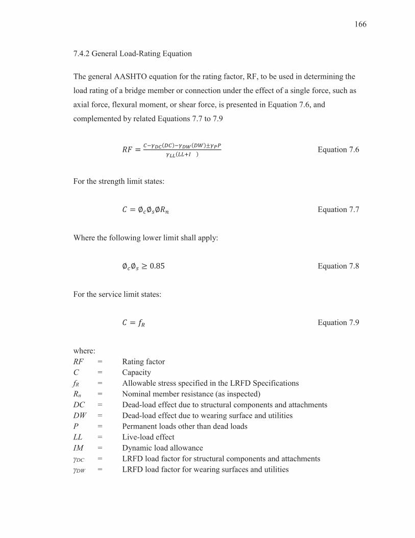
166
7.4.2 General Load-Rating Equation
The general AASHTO equation for the rating factor, RF, to be used in determining the
load rating of a bridge member or connection under the effect of a single force, such as
axial force, flexural moment, or shear force, is presented in Equation 7.6, and
complemented by related Equations 7.7 to 7.9
�� ���� !"#�$�� %"#&$'�()
�**"++,- $ Equation 7.6
For the strength limit states:
. � ∅0∅1∅�2 Equation 7.7
Where the following lower limit shall apply:
∅0∅1 3 0.85 Equation 7.8
For the service limit states:
. � 79 Equation 7.9
where:
RF = Rating factor
C = Capacity
fR = Allowable stress specified in the LRFD Specifications
Rn = Nominal member resistance (as inspected)
DC = Dead-load effect due to structural components and attachments
DW = Dead-load effect due to wearing surface and utilities
P = Permanent loads other than dead loads
LL = Live-load effect
IM = Dynamic load allowance
γDC = LRFD load factor for structural components and attachments
γDW = LRFD load factor for wearing surfaces and utilities

167
γP = LRFD load factor for permanent loads other than dead loads = 1.0
γLL = Evaluation live-load factor
øc = Condition factor
øs = System factor
ø = LRFD resistance factor
When the permanent loads other than dead loads, P, are not considered, the general
equation is reduced to the Equation 7.10
�� ���� !"#�$��%&"#'$
�(("))*+,$ Equation 7.10
Equation 7.10 was the expression used in this research to evaluate the load rating factor
for the series of selected bridges. The load rating was performed to each applicable limit
state and load effect, being the lowest value the controlling rating factor (AASHTO,
2011). According to AASHTO MBE (AASHTO, 2011) “The condition factor øc provides
a reduction to account for the increased uncertainty in the resistance of deteriorated
members and the likely increased future deterioration of these members during the period
between inspection cycles. The condition factors are presented in AASHTO Table
6A.4.2.3-1. The system factors øs are multipliers applied to the nominal resistance to
reflect the level of redundancy of the complete superstructure system. The system factors
are presented in AASHTO Table 6A.4.2.4-1.” The resistant factor ø for bending and
shear effects were taken as 1.0. The variability of load effects is included by the load
factor γ, which is related to the uncertainties of load magnitude, loads position, and
possible load combinations. As a limit state involves the effect of different load types and
each load is estimated with different uncertainty, the total load effect is the sum of each
load affected by its corresponding load factor. The load factors for load rating are
presented in Table 6A.4.2.2-1 from the AASHTO MBE (2011).

168
7.4.3 Levels of Evaluation
The AASHTO MBE (2011) specifies three levels of live load rating, which have to be
performed in a sequential manner, based on the owner needs. The first stage is the
design-load rating, followed by the legal-load rating, and ending with the permit-load
rating. The permit-load rating checks the safety and serviceability performance of a
bridge under the passage of a special truck, exceeding the legal weight limitations. This is
a very specialized bridge consideration that is not applicable to all bridges, and therefore,
permit-load rating was not considered in this research. Therefore, only design-load and
legal-load rating were performed in this study to all the considered bridge models.
7.4.3.1 Design-load rating
Design-load rating is the first level of evaluation of bridges and it is based on the HL-93
loading and the requirements from LRFD design standards. The assessment uses the
actual section dimensions and material properties, as recorded during the most recent
field inspection. This evaluation is a measure of performance of existing bridges to
current LRFD bridge design standards. The live load rating at this stage can be performed
at the same design level of reliability, known as Inventory level, for new bridges
according to AASHTO LRFD (2012). Also the bridges can be assessed at a lower level of
reliability equivalent to the Operating level, based on past load-rating practice. The
design-load rating calculates Inventory and Operating rating factors for the LRFD-design
live load HL-93. Strength I and Serviceability II limit states should be verified. The
design live load HL-93 was presented in Figure 7.1.
7.4.3.2 Legal-load rating
Bridges without enough structural capacity under the design-load rating (RF < 1.0)
should be analyzed for legal loads in order to establish the need for load posting or bridge
repair or rehabilitation. Legal loads consist of:

169
· The AASHTO family of three legal loads (Type 3, Type 3S2 and Type 3-3) and lane
type load, presented in Figure 7.14. The AASHTO legal vehicles and lane type load
are used in load rating bridges for routine commercial traffic.
· The four specialized hauling vehicles (SHVs) presented in Figure 7.15, or the Notional
rating load (NRL) which envelopes the SHVs configuration and is shown in Figure
7.16.
· Any specialized legal loads developed by individual states that are appropriate for use
within their state and under their jurisdiction.
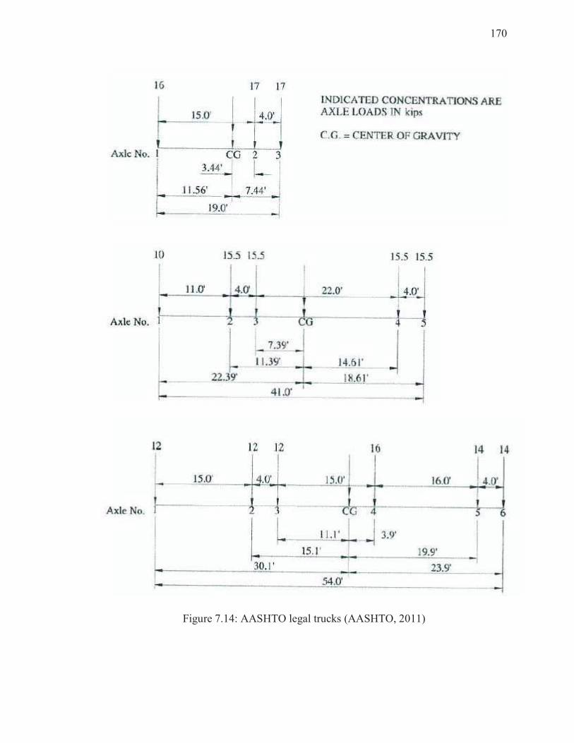
170
Figure 7.14: AASHTO legal trucks (AASHTO, 2011)
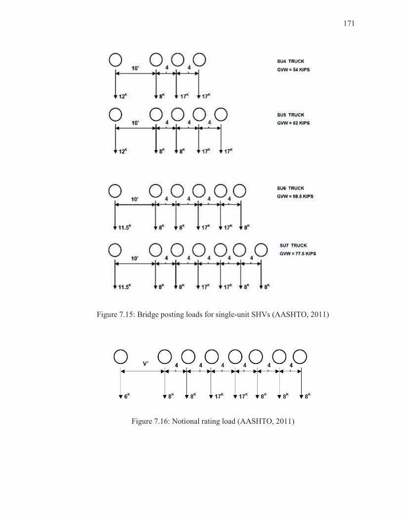
171
Figure 7.15: Bridge posting loads for single-unit SHVs (AASHTO, 2011)
Figure 7.16: Notional rating load (AASHTO, 2011)
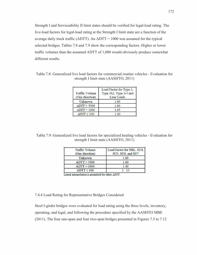
172
Strength I and Serviceability II limit states should be verified for legal-load rating. The
live-load factors for legal-load rating at the Strength I limit state are a function of the
average daily truck traffic (ADTT). An ADTT = 1000 was assumed for the typical
selected bridges. Tables 7.8 and 7.9 show the corresponding factors. Higher or lower
traffic volumes than the assumed ADTT of 1,000 would obviously produce somewhat
different results.
Tabla 7.8: Generalized live load factors for commercial routine vehicles - Evaluation for strength I limit state (AASHTO, 2011)
Tabla 7.9: Generalized live load factors for specialized hauling vehicles - Evaluation for strength I limit state (AASHTO, 2011)
7.4.4 Load Rating for Representative Bridges Considered
Steel I-girder bridges were evaluated for load rating using the three levels, inventory,
operating, and legal, and following the procedure specified by the AASHTO MBE
(2011). The four one-span and four two-span bridges presented in Figures 7.5 to 7.12
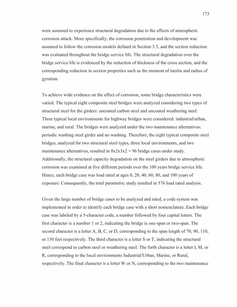
173
were assumed to experience structural degradation due to the effects of atmospheric
corrosion attack. More specifically, the corrosion penetration and development was
assumed to follow the corrosion models defined in Section 3.5, and the section reduction
was evaluated throughout the bridge service life. The structural degradation over the
bridge service life is evidenced by the reduction of thickness of the cross section, and the
corresponding reduction in section properties such as the moment of inertia and radius of
gyration.
To achieve wide evidence on the effect of corrosion, some bridge characteristics were
varied. The typical eight composite steel bridges were analyzed considering two types of
structural steel for the girders: uncoated carbon steel and uncoated weathering steel.
Three typical local environments for highway bridges were considered: industrial/urban,
marine, and rural. The bridges were analyzed under the two maintenance alternatives:
periodic washing steel girder and no washing. Therefore, the eight typical composite steel
bridges, analyzed for two structural steel types, three local environments, and two
maintenance alternatives, resulted in 8x2x3x2 = 96 bridge cases under study.
Additionally, the structural capacity degradation on the steel girders due to atmospheric
corrosion was examined at five different periods over the 100 years bridge service life.
Hence, each bridge case was load rated at ages 0, 20, 40, 60, 80, and 100 years of
exposure. Consequently, the total parametric study resulted in 576 load rated analysis.
Given the large number of bridge cases to be analyzed and rated, a code system was
implemented in order to identify each bridge case with a short nomenclature. Each bridge
case was labeled by a 5-character code, a number followed by four capital letters. The
first character is a number 1 or 2, indicating the bridge is one-span or two-span. The
second character is a letter A, B, C, or D, corresponding to the span length of 70, 90, 110,
or 130 feet respectively. The third character is a letter S or T, indicating the structural
steel correspond to carbon steel or weathering steel. The forth character is a letter I, M, or
R, corresponding to the local environments Industrial/Urban, Marine, or Rural,
respectively. The final character is a letter W or N, corresponding to the two maintenance
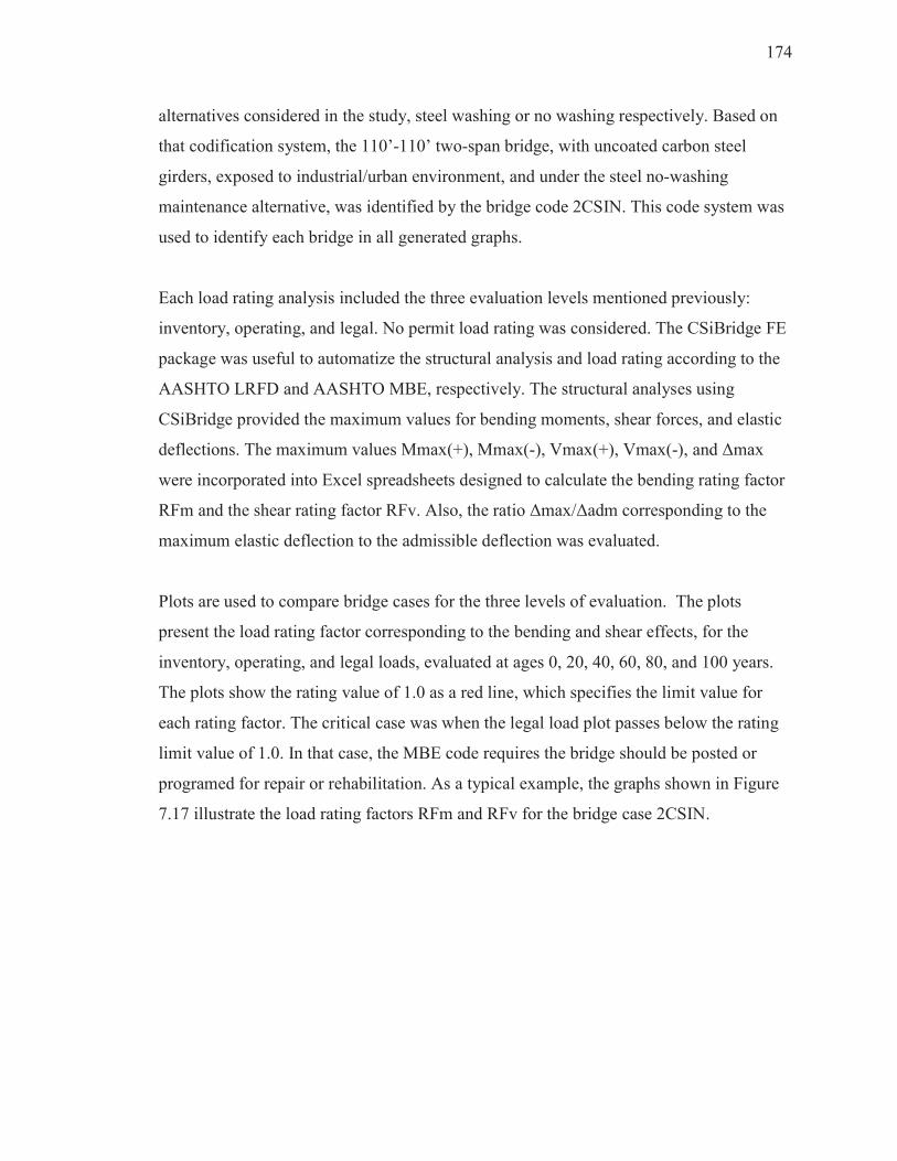
174
alternatives considered in the study, steel washing or no washing respectively. Based on
that codification system, the 110’-110’ two-span bridge, with uncoated carbon steel
girders, exposed to industrial/urban environment, and under the steel no-washing
maintenance alternative, was identified by the bridge code 2CSIN. This code system was
used to identify each bridge in all generated graphs.
Each load rating analysis included the three evaluation levels mentioned previously:
inventory, operating, and legal. No permit load rating was considered. The CSiBridge FE
package was useful to automatize the structural analysis and load rating according to the
AASHTO LRFD and AASHTO MBE, respectively. The structural analyses using
CSiBridge provided the maximum values for bending moments, shear forces, and elastic
deflections. The maximum values Mmax(+), Mmax(-), Vmax(+), Vmax(-), and Δmax
were incorporated into Excel spreadsheets designed to calculate the bending rating factor
RFm and the shear rating factor RFv. Also, the ratio Δmax/Δadm corresponding to the
maximum elastic deflection to the admissible deflection was evaluated.
Plots are used to compare bridge cases for the three levels of evaluation. The plots
present the load rating factor corresponding to the bending and shear effects, for the
inventory, operating, and legal loads, evaluated at ages 0, 20, 40, 60, 80, and 100 years.
The plots show the rating value of 1.0 as a red line, which specifies the limit value for
each rating factor. The critical case was when the legal load plot passes below the rating
limit value of 1.0. In that case, the MBE code requires the bridge should be posted or
programed for repair or rehabilitation. As a typical example, the graphs shown in Figure
7.17 illustrate the load rating factors RFm and RFv for the bridge case 2CSIN.
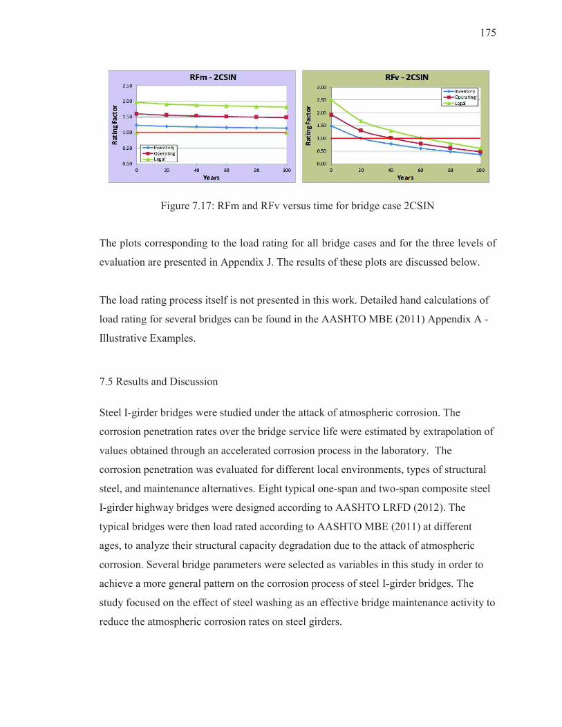
175
Figure 7.17: RFm and RFv versus time for bridge case 2CSIN
The plots corresponding to the load rating for all bridge cases and for the three levels of
evaluation are presented in Appendix J. The results of these plots are discussed below.
The load rating process itself is not presented in this work. Detailed hand calculations of
load rating for several bridges can be found in the AASHTO MBE (2011) Appendix A -
Illustrative Examples.
7.5 Results and Discussion
Steel I-girder bridges were studied under the attack of atmospheric corrosion. The
corrosion penetration rates over the bridge service life were estimated by extrapolation of
values obtained through an accelerated corrosion process in the laboratory. The
corrosion penetration was evaluated for different local environments, types of structural
steel, and maintenance alternatives. Eight typical one-span and two-span composite steel
I-girder highway bridges were designed according to AASHTO LRFD (2012). The
typical bridges were then load rated according to AASHTO MBE (2011) at different
ages, to analyze their structural capacity degradation due to the attack of atmospheric
corrosion. Several bridge parameters were selected as variables in this study in order to
achieve a more general pattern on the corrosion process of steel I-girder bridges. The
study focused on the effect of steel washing as an effective bridge maintenance activity to
reduce the atmospheric corrosion rates on steel girders.
176
The load rating analysis followed the requirements stipulated in the AASHTO MBE
(2011), using the time dependent corrosion penetration rates, corrosion section model,
typical steel highway bridges configuration, and structural parameters previously defined
for this research. The basic procedure was to evaluate: 1) the thickness reduction for web
and bottom flange of girder sections at selected ages (0, 20, 40, 60, 80, and 100 years), 2)
the bridge section properties at selected ages, 3) the structural capacity for bending and
shear effects at each selected age, and 4) the corresponding rating factors RFm and RFv
at those selected ages. According to the AASHTO MBE (2011) a bridge should be posted
when the maximum effect due to legal load exceeds the safe load capacity of a bridge
member (RF < 1.0). In that case the bridge is allowed to service only to a maximum live
load corresponding to the legal load times the legal rating factor (posting), otherwise the
bridge should be closed for rehabilitation/repair. Legal loads to be analyzed were
presented in the previous section. Posting a bridge can create serious restrictions and limit
the passage of truck traffic.
The parametric load rating analysis on the selected bridge cases included the following
variables: number of spans (one or two), span length (70, 90, 110, and 130 feet), steel
type (carbon steel or weathering steel), local environment (Industrial/urban, Marine, and
Rural), and maintenance alternative (steel washing or no washing). These variables were
applied to the typical eight bridge models selected. The data obtained from the load rating
analyses were processed and evaluated using spreadsheets from Microsoft Excel. This
tool was used to process the abundant data from each bridge analysis at each defined age,
such us: 1) section properties, 2) maximum moment and shear effects, and maximum
elastic deflections due to dead load DC1, DC2, and DW, 3) maximum moment and shear
effects, and maximum elastic deflections due to live load LL+IM for operating loads,
inventory loads, and legal loads, and 4) nominal moment and shear capacity, and
permissible elastic deflections. The final results were the values of rating factors for
bending and shear effects RFm and RFv respectively, for each load level (inventory,
operating, and legal) and at each selected age. After all calculations were completed, the
177
results were processed and summarized in a series of plots, which are shown in Appendix
J. Some trends and interpretations for the results are summarized below.
7.5.1 Effect of Stress Type
The reduction of moment and shear capacities due to atmospheric corrosion attack was
observed in all of the load rating analyses. In general, it was found that the bridge
bending capacity reduces at a low rate during its service life. In contrast, the bridge shear
capacity was found to reduce faster over time. The design conditions of the typical bridge
sections utilized elements that were compact sections, with slenderness ratios lower than
the maximum values prescribed by the AASHTO LRFD Specifications. The selected
bridge cases were analyzed at different ages of their service lives, showing incremental
progress of the corrosion penetration with time, and consequently, a reduction on the
thicknesses of the section. The corrosion process changed the initial condition of some
elements, as the slenderness ratios of web and flanges. Three important facts on the steel
girders design and the atmospheric corrosion attack were: 1) the web thickness was
always thinner than the flanges thickness, 2) the section deterioration model considered
corrosion on both web faces, and 3) the section deterioration model considered flange
corrosion only on the top faces of the bottom flange. The assumed corrosion behavior
reduced dramatically the section shear capacity, mainly provided by the web area. On the
other hand, the bottom flange thickness reduced considerably less than that of the web.
As a consequence, the section moment capacity, which is mainly generated by the flanges
area, was reduced at a lower rate.
Figure 7.18 presents the RFm and RFv factors due to bending and shear stresses
respectively, for the three levels of evaluation: inventory, operating, and legal, and for the
two steel types considered. In Figure 7.18 (left) the results are presented for the rating
analysis for the bridge case 1ASIN (one-span, 70’ span length, carbon steel type,
industrial/urban local environment, and no washing alternative), while in Figure 7.18
(right) the corresponding results are shown for bridge 1ASIW, which is equivalent to the

178
previous bridge case, but for the steel washing alternative. Figure 7.18 (left and right)
illustrate how quickly the RFv (solid line) decrease with time in comparison to RFm
(dotted line) reduction. The RFv reduction for the three levels of evaluation show a
similar pattern, with the three curves quite parallel. As indicated, the RFm reduces at a
lower rate but they also present a similar pattern, with the three curves almost parallel.
In Figure 7.19 (left) the load rating results for the bridge case 2CTMN (two-span, 110’-
110’ span length, weathering steel, marine local environment, and no washing
alternative) are shown. Figure 7.19 (right) meanwhile shows the results for bridge case
2CTMW, which is the same as the previous bridge but for the steel washing alternative.
The two bridge cases presented in Figure 7.19 included different parameters than those
presented in Figure 7.18, but still demonstrate the same pattern, with RFv (solid line)
reducing more rapidly with time than RFm (dotted line), and with rating curves almost
parallel as noted in Figure 7.18. The parallel pattern for RFm and RFv curves was
marked by the difference on the bridge structural capacity at age zero. This pattern was
the same for both one-span and two-span bridge cases.
In the four cases presented in Figures 7.18 and 7.19, it can be seen that the rating factors
for inventory level were the lowest, followed by the operating rating factors, and lastly by
the legal rating factors, which were the highest values. This pattern remained the same in
all the analyzed cases, as expected, since the inventory level was the most demanding
evaluation, followed for the operating level, and ending with the legal level as the least
demanding. Based on this general pattern, the rest of analyses were performed only
focusing on the RFm and RFv factors for legal-load level, since this is the trigger level
for posting or closing a bridge for repair/rehabilitation. The bending capacity reduced at a
very low rate, and consequently the RFm parameter never reached the limit value of 1.0
during the entire bridge service life. At the other hand, the shear capacity drooped at a
deep ratio, and hence the RFv parameter reached the limit of 1.0 for several bridge cases.
Therefore, the shear capacity degradation, expressed by the drop of the RFv parameter, is
analyzed in more detail in the next sections.
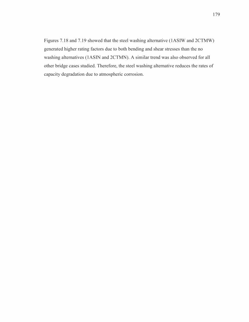
179
Figures 7.18 and 7.19 showed that the steel washing alternative (1ASIW and 2CTMW)
generated higher rating factors due to both bending and shear stresses than the no
washing alternatives (1ASIN and 2CTMN). A similar trend was also observed for all
other bridge cases studied. Therefore, the steel washing alternative reduces the rates of
capacity degradation due to atmospheric corrosion.
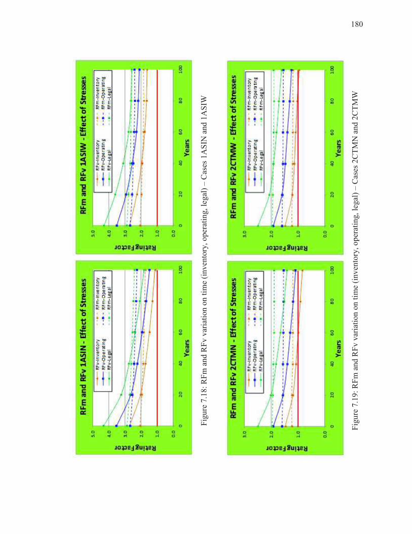
180
Fig
ure
7.1
8:
RF
m a
nd
RF
v v
aria
tio
n o
n t
ime
(in
ven
tory
, o
per
atin
g,
leg
al)
– C
ases
1A
SIN
and
1A
SIW
Fig
ure
7.1
9:
RF
m a
nd
RF
v v
aria
tio
n o
n t
ime
(in
ven
tory
, o
per
atin
g,
leg
al)
– C
ases
2C
TM
N a
nd
2C
TM
W

181
7.5.2 Effect of Local Environment
A general pattern for all bridge cases analyzed in this study showed that local
industrial/urban environment always produced the higher structural capacity degradation
for both bending and shear effects due to atmospheric corrosion attack. The local marine
environment resulted in the second most aggressive local environment for both bending
and shear effects. The local rural environment was the least aggressive condition for all
analyzed cases.
Figure 7.20 shows the plots for RFv factors for two sets of bridge cases from weathering
steel and for legal load level. One set conformed to the three bridge cases (1AT_N, solid
lines) corresponding to bridge cases of one-span, 70’ span length, weathering steel type,
no washing alternative, and exposed to the three possible environments: industrial/urban,
marine, or rural. The second set of bridge cases correspond to the same three previous
bridge cases indicated, but for the steel washing alternative (1AT_W, dotted lines). The
plots show a general pattern for the six considered cases, with industrial/marine as the
most aggressive environment, followed by the marine environment, and the rural
environment as the less aggressive local environment.
Figure 7.21 shows the plots for RFv factors for two more sets of bridge from cases from
carbon steel and for legal load level. One set consisted by the three bridge cases (2BT_N,
solid lines) corresponding to bridge cases of two-span, 90’ equal span length, weathering
steel type, no washing alternative, and exposed to the three possible environments:
industrial/urban, marine, or rural. The second set of bridge cases correspond to the same
three previous bridge cases indicated, but for the steel washing alternative (2BT_W,
dotted lines). The plots show the same general pattern as in Figure 7.20, with
industrial/urban as the most aggressive environment, followed by the marine
environment, and the rural environment as the less aggressive environment.
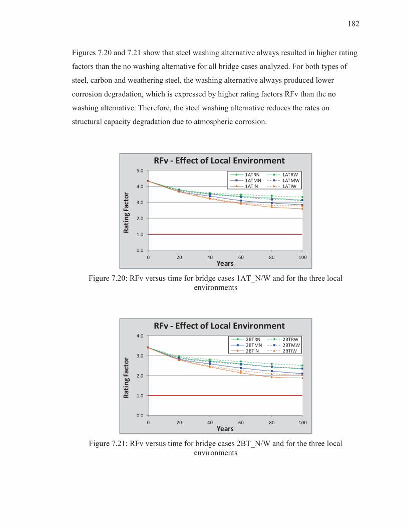
182
Figures 7.20 and 7.21 show that steel washing alternative always resulted in higher rating
factors than the no washing alternative for all bridge cases analyzed. For both types of
steel, carbon and weathering steel, the washing alternative always produced lower
corrosion degradation, which is expressed by higher rating factors RFv than the no
washing alternative. Therefore, the steel washing alternative reduces the rates on
structural capacity degradation due to atmospheric corrosion.
Figure 7.20: RFv versus time for bridge cases 1AT_N/W and for the three local environments
Figure 7.21: RFv versus time for bridge cases 2BT_N/W and for the three local environments
0.0
1.0
2.0
3.0
4.0
5.0
0 20 40 60 80 100
Ra
tin
g F
act
or
Years
RFv - Effect of Local Environment
1ATRN 1ATRW1ATMN 1ATMW1ATIN 1ATIW
0.0
1.0
2.0
3.0
4.0
0 20 40 60 80 100
Ra
tin
g F
act
or
Years
RFv - Effect of Local Environment
2BTRN 2BTRW2BTMN 2BTMW2BTIN 2BTIW
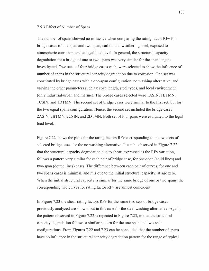
183
7.5.3 Effect of Number of Spans
The number of spans showed no influence when comparing the rating factor RFv for
bridge cases of one-span and two-span, carbon and weathering steel, exposed to
atmospheric corrosion, and at legal load level. In general, the structural capacity
degradation for a bridge of one or two-spans was very similar for the span lengths
investigated. Two sets, of four bridge cases each, were selected to show the influence of
number of spans in the structural capacity degradation due to corrosion. One set was
constituted by bridge cases with a one-span configuration, no washing alternative, and
varying the other parameters such as: span length, steel types, and local environment
(only industrial/urban and marine). The bridge cases selected were 1ASIN, 1BTMN,
1CSIN, and 1DTMN. The second set of bridge cases were similar to the first set, but for
the two equal spans configuration. Hence, the second set included the bridge cases
2ASIN, 2BTMN, 2CSIN, and 2DTMN. Both set of four pairs were evaluated to the legal
load level.
Figure 7.22 shows the plots for the rating factors RFv corresponding to the two sets of
selected bridge cases for the no washing alternative. It can be observed in Figure 7.22
that the structural capacity degradation due to shear, expressed as the RFv variation,
follows a pattern very similar for each pair of bridge case, for one-span (solid lines) and
two-span (dotted lines) cases. The difference between each pair of curves, for one and
two spans cases is minimal, and it is due to the initial structural capacity, at age zero.
When the initial structural capacity is similar for the same bridge of one or two spans, the
corresponding two curves for rating factor RFv are almost coincident.
In Figure 7.23 the shear rating factors RFv for the same two sets of bridge cases
previously analyzed are shown, but in this case for the steel washing alternative. Again,
the pattern observed in Figure 7.22 is repeated in Figure 7.23, in that the structural
capacity degradation follows a similar pattern for the one-span and two-span
configurations. From Figures 7.22 and 7.23 can be concluded that the number of spans
have no influence in the structural capacity degradation pattern for the range of typical
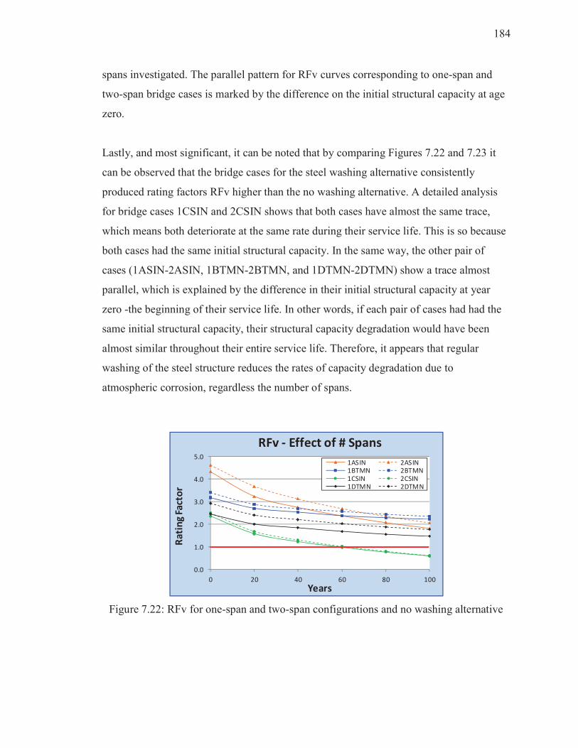
184
spans investigated. The parallel pattern for RFv curves corresponding to one-span and
two-span bridge cases is marked by the difference on the initial structural capacity at age
zero.
Lastly, and most significant, it can be noted that by comparing Figures 7.22 and 7.23 it
can be observed that the bridge cases for the steel washing alternative consistently
produced rating factors RFv higher than the no washing alternative. A detailed analysis
for bridge cases 1CSIN and 2CSIN shows that both cases have almost the same trace,
which means both deteriorate at the same rate during their service life. This is so because
both cases had the same initial structural capacity. In the same way, the other pair of
cases (1ASIN-2ASIN, 1BTMN-2BTMN, and 1DTMN-2DTMN) show a trace almost
parallel, which is explained by the difference in their initial structural capacity at year
zero -the beginning of their service life. In other words, if each pair of cases had had the
same initial structural capacity, their structural capacity degradation would have been
almost similar throughout their entire service life. Therefore, it appears that regular
washing of the steel structure reduces the rates of capacity degradation due to
atmospheric corrosion, regardless the number of spans.
Figure 7.22: RFv for one-span and two-span configurations and no washing alternative
0.0
1.0
2.0
3.0
4.0
5.0
0 20 40 60 80 100
Ra
tin
g F
act
or
Years
RFv - Effect of # Spans
1ASIN 2ASIN1BTMN 2BTMN1CSIN 2CSIN1DTMN 2DTMN
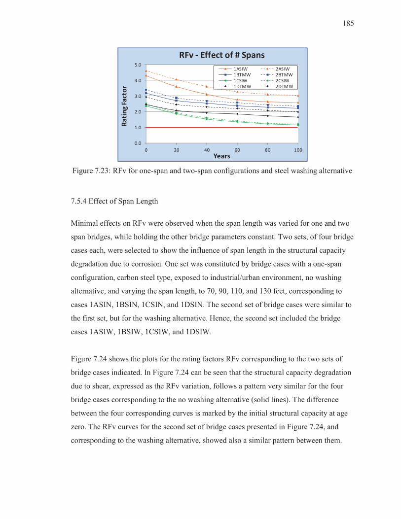
185
Figure 7.23: RFv for one-span and two-span configurations and steel washing alternative
7.5.4 Effect of Span Length
Minimal effects on RFv were observed when the span length was varied for one and two
span bridges, while holding the other bridge parameters constant. Two sets, of four bridge
cases each, were selected to show the influence of span length in the structural capacity
degradation due to corrosion. One set was constituted by bridge cases with a one-span
configuration, carbon steel type, exposed to industrial/urban environment, no washing
alternative, and varying the span length, to 70, 90, 110, and 130 feet, corresponding to
cases 1ASIN, 1BSIN, 1CSIN, and 1DSIN. The second set of bridge cases were similar to
the first set, but for the washing alternative. Hence, the second set included the bridge
cases 1ASIW, 1BSIW, 1CSIW, and 1DSIW.
Figure 7.24 shows the plots for the rating factors RFv corresponding to the two sets of
bridge cases indicated. In Figure 7.24 can be seen that the structural capacity degradation
due to shear, expressed as the RFv variation, follows a pattern very similar for the four
bridge cases corresponding to the no washing alternative (solid lines). The difference
between the four corresponding curves is marked by the initial structural capacity at age
zero. The RFv curves for the second set of bridge cases presented in Figure 7.24, and
corresponding to the washing alternative, showed also a similar pattern between them.
0.0
1.0
2.0
3.0
4.0
5.0
0 20 40 60 80 100
Ra
tin
g F
act
or
Years
RFv - Effect of # Spans
1ASIW 2ASIW1BTMW 2BTMW
1CSIW 2CSIW1DTMW 2DTMW
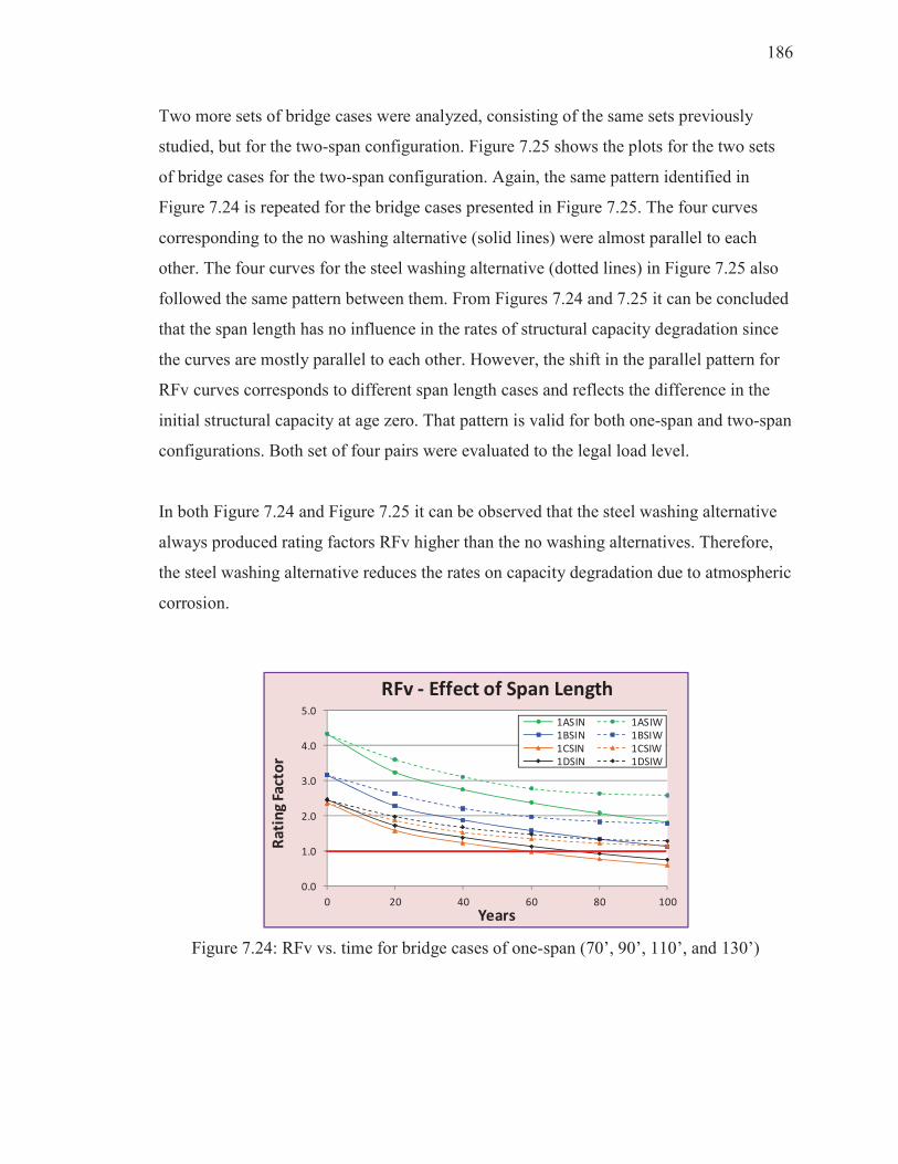
186
Two more sets of bridge cases were analyzed, consisting of the same sets previously
studied, but for the two-span configuration. Figure 7.25 shows the plots for the two sets
of bridge cases for the two-span configuration. Again, the same pattern identified in
Figure 7.24 is repeated for the bridge cases presented in Figure 7.25. The four curves
corresponding to the no washing alternative (solid lines) were almost parallel to each
other. The four curves for the steel washing alternative (dotted lines) in Figure 7.25 also
followed the same pattern between them. From Figures 7.24 and 7.25 it can be concluded
that the span length has no influence in the rates of structural capacity degradation since
the curves are mostly parallel to each other. However, the shift in the parallel pattern for
RFv curves corresponds to different span length cases and reflects the difference in the
initial structural capacity at age zero. That pattern is valid for both one-span and two-span
configurations. Both set of four pairs were evaluated to the legal load level.
In both Figure 7.24 and Figure 7.25 it can be observed that the steel washing alternative
always produced rating factors RFv higher than the no washing alternatives. Therefore,
the steel washing alternative reduces the rates on capacity degradation due to atmospheric
corrosion.
Figure 7.24: RFv vs. time for bridge cases of one-span (70’, 90’, 110’, and 130’)
0.0
1.0
2.0
3.0
4.0
5.0
0 20 40 60 80 100
Ra
tin
g F
act
or
Years
RFv - Effect of Span Length
1ASIN 1ASIW1BSIN 1BSIW
1CSIN 1CSIW1DSIN 1DSIW
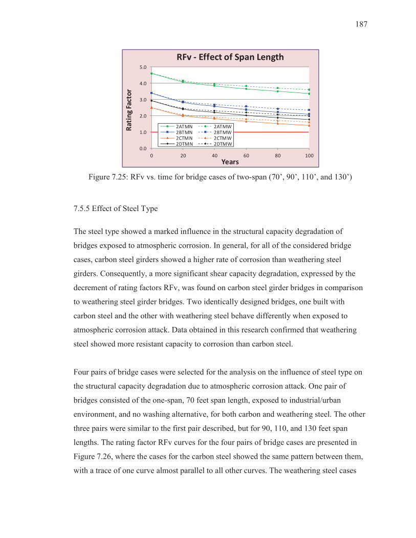
187
Figure 7.25: RFv vs. time for bridge cases of two-span (70’, 90’, 110’, and 130’)
7.5.5 Effect of Steel Type
The steel type showed a marked influence in the structural capacity degradation of
bridges exposed to atmospheric corrosion. In general, for all of the considered bridge
cases, carbon steel girders showed a higher rate of corrosion than weathering steel
girders. Consequently, a more significant shear capacity degradation, expressed by the
decrement of rating factors RFv, was found on carbon steel girder bridges in comparison
to weathering steel girder bridges. Two identically designed bridges, one built with
carbon steel and the other with weathering steel behave differently when exposed to
atmospheric corrosion attack. Data obtained in this research confirmed that weathering
steel showed more resistant capacity to corrosion than carbon steel.
Four pairs of bridge cases were selected for the analysis on the influence of steel type on
the structural capacity degradation due to atmospheric corrosion attack. One pair of
bridges consisted of the one-span, 70 feet span length, exposed to industrial/urban
environment, and no washing alternative, for both carbon and weathering steel. The other
three pairs were similar to the first pair described, but for 90, 110, and 130 feet span
lengths. The rating factor RFv curves for the four pairs of bridge cases are presented in
Figure 7.26, where the cases for the carbon steel showed the same pattern between them,
with a trace of one curve almost parallel to all other curves. The weathering steel cases
0.0
1.0
2.0
3.0
4.0
5.0
0 20 40 60 80 100
Ra
tin
g F
act
or
Years
RFv - Effect of Span Length
2ATMN 2ATMW2BTMN 2BTMW2CTMN 2CTMW2DTMN 2DTMW
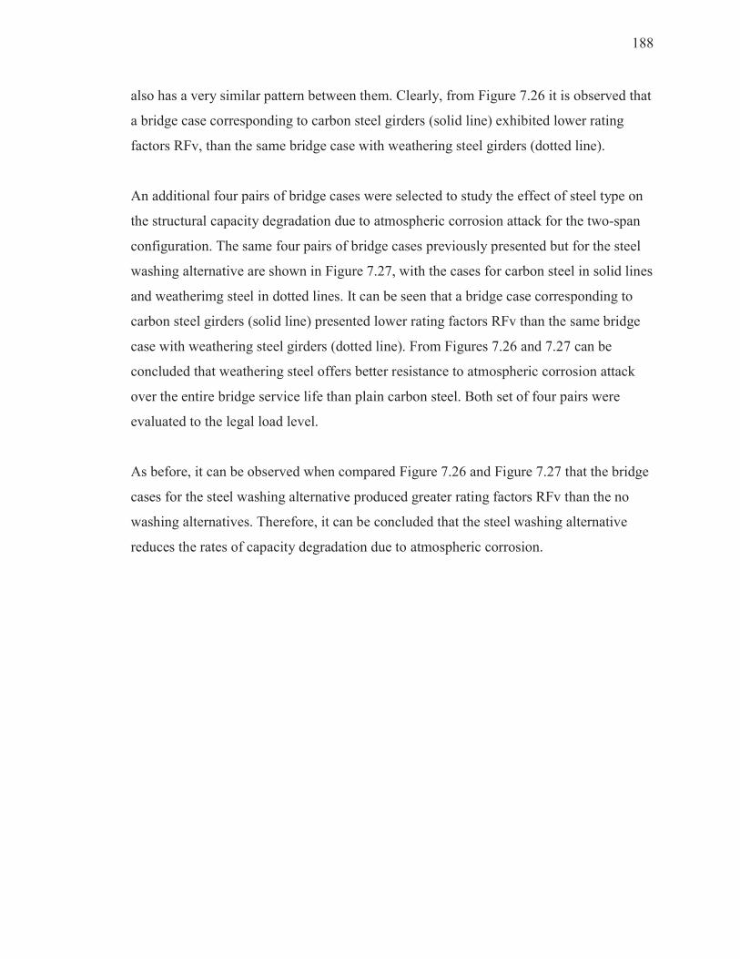
188
also has a very similar pattern between them. Clearly, from Figure 7.26 it is observed that
a bridge case corresponding to carbon steel girders (solid line) exhibited lower rating
factors RFv, than the same bridge case with weathering steel girders (dotted line).
An additional four pairs of bridge cases were selected to study the effect of steel type on
the structural capacity degradation due to atmospheric corrosion attack for the two-span
configuration. The same four pairs of bridge cases previously presented but for the steel
washing alternative are shown in Figure 7.27, with the cases for carbon steel in solid lines
and weatherimg steel in dotted lines. It can be seen that a bridge case corresponding to
carbon steel girders (solid line) presented lower rating factors RFv than the same bridge
case with weathering steel girders (dotted line). From Figures 7.26 and 7.27 can be
concluded that weathering steel offers better resistance to atmospheric corrosion attack
over the entire bridge service life than plain carbon steel. Both set of four pairs were
evaluated to the legal load level.
As before, it can be observed when compared Figure 7.26 and Figure 7.27 that the bridge
cases for the steel washing alternative produced greater rating factors RFv than the no
washing alternatives. Therefore, it can be concluded that the steel washing alternative
reduces the rates of capacity degradation due to atmospheric corrosion.
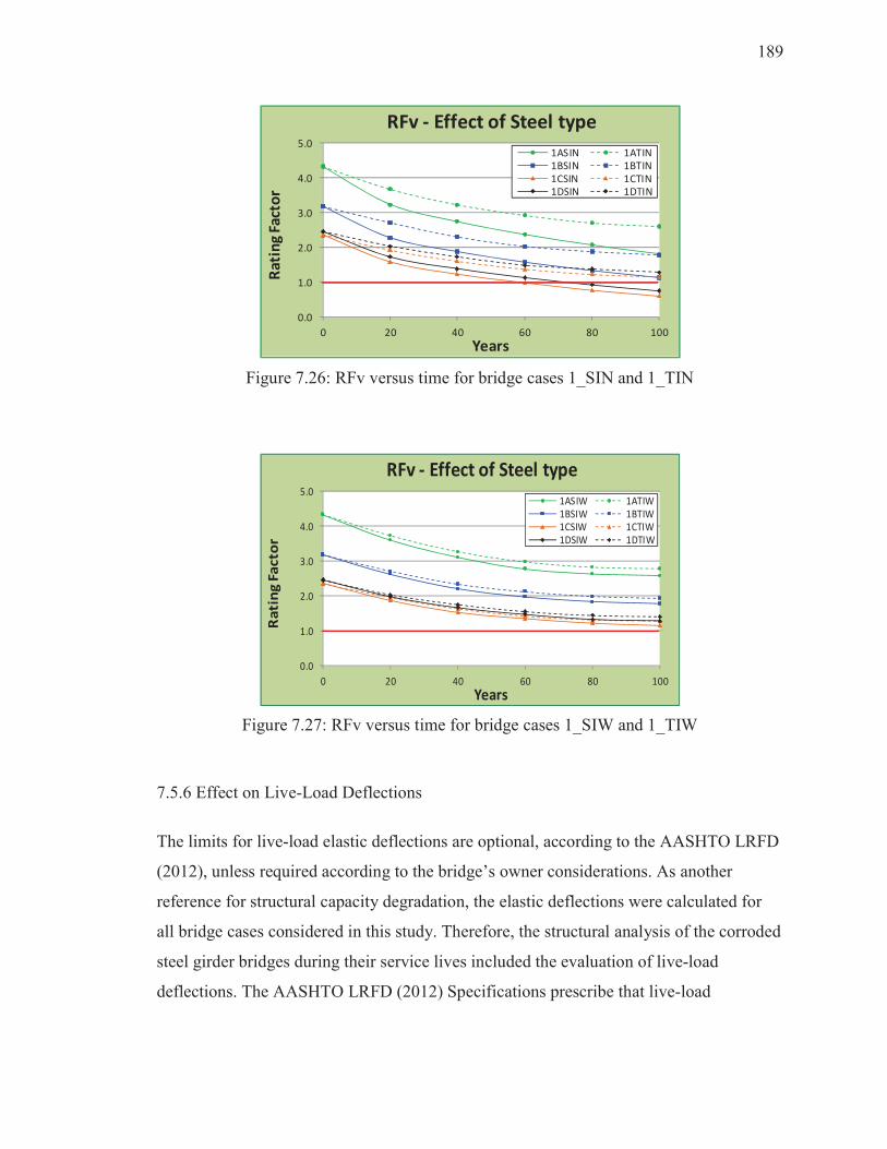
189
Figure 7.26: RFv versus time for bridge cases 1_SIN and 1_TIN
0.0
1.0
2.0
3.0
4.0
5.0
0 20 40 60 80 100
Ra
tin
g F
acto
r
Years
RFv - Effect of Steel type
1ASIW 1ATIW1BSIW 1BTIW1CSIW 1CTIW1DSIW 1DTIW
Figure 7.27: RFv versus time for bridge cases 1_SIW and 1_TIW
7.5.6 Effect on Live-Load Deflections
The limits for live-load elastic deflections are optional, according to the AASHTO LRFD
(2012), unless required according to the bridge’s owner considerations. As another
reference for structural capacity degradation, the elastic deflections were calculated for
all bridge cases considered in this study. Therefore, the structural analysis of the corroded
steel girder bridges during their service lives included the evaluation of live-load
deflections. The AASHTO LRFD (2012) Specifications prescribe that live-load
0.0
1.0
2.0
3.0
4.0
5.0
0 20 40 60 80 100
Ra
tin
g F
act
or
Years
RFv - Effect of Steel type
1ASIN 1ATIN1BSIN 1BTIN
1CSIN 1CTIN1DSIN 1DTIN
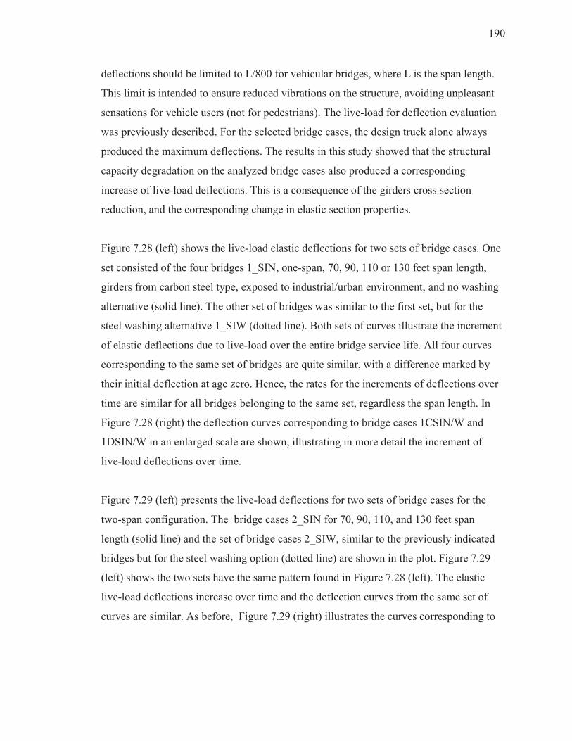
190
deflections should be limited to L/800 for vehicular bridges, where L is the span length.
This limit is intended to ensure reduced vibrations on the structure, avoiding unpleasant
sensations for vehicle users (not for pedestrians). The live-load for deflection evaluation
was previously described. For the selected bridge cases, the design truck alone always
produced the maximum deflections. The results in this study showed that the structural
capacity degradation on the analyzed bridge cases also produced a corresponding
increase of live-load deflections. This is a consequence of the girders cross section
reduction, and the corresponding change in elastic section properties.
Figure 7.28 (left) shows the live-load elastic deflections for two sets of bridge cases. One
set consisted of the four bridges 1_SIN, one-span, 70, 90, 110 or 130 feet span length,
girders from carbon steel type, exposed to industrial/urban environment, and no washing
alternative (solid line). The other set of bridges was similar to the first set, but for the
steel washing alternative 1_SIW (dotted line). Both sets of curves illustrate the increment
of elastic deflections due to live-load over the entire bridge service life. All four curves
corresponding to the same set of bridges are quite similar, with a difference marked by
their initial deflection at age zero. Hence, the rates for the increments of deflections over
time are similar for all bridges belonging to the same set, regardless the span length. In
Figure 7.28 (right) the deflection curves corresponding to bridge cases 1CSIN/W and
1DSIN/W in an enlarged scale are shown, illustrating in more detail the increment of
live-load deflections over time.
Figure 7.29 (left) presents the live-load deflections for two sets of bridge cases for the
two-span configuration. The bridge cases 2_SIN for 70, 90, 110, and 130 feet span
length (solid line) and the set of bridge cases 2_SIW, similar to the previously indicated
bridges but for the steel washing option (dotted line) are shown in the plot. Figure 7.29
(left) shows the two sets have the same pattern found in Figure 7.28 (left). The elastic
live-load deflections increase over time and the deflection curves from the same set of
curves are similar. As before, Figure 7.29 (right) illustrates the curves corresponding to

191
bridge cases 2CSIN/W and 2DSIN/W in an enlarged scale, where more detail of the
increment of live-load deflections over time can be observed.
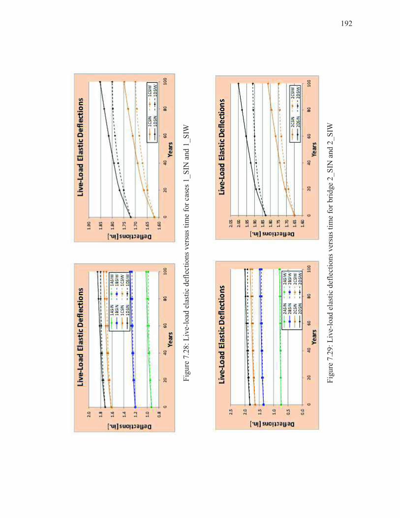
192
Fig
ure
7.2
8:
Liv
e-lo
ad e
last
ic d
efle
ctio
ns
ver
sus
tim
e fo
r ca
ses
1_
SIN
and
1_
SIW
Fig
ure
7.2
9:
Liv
e-lo
ad e
last
ic d
efle
ctio
ns
ver
sus
tim
e fo
r b
rid
ge
2_
SIN
and
2_
SIW
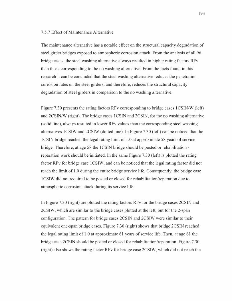
193
7.5.7 Effect of Maintenance Alternative
The maintenance alternative has a notable effect on the structural capacity degradation of
steel girder bridges exposed to atmospheric corrosion attack. From the analysis of all 96
bridge cases, the steel washing alternative always resulted in higher rating factors RFv
than those corresponding to the no washing alternative. From the facts found in this
research it can be concluded that the steel washing alternative reduces the penetration
corrosion rates on the steel girders, and therefore, reduces the structural capacity
degradation of steel girders in comparison to the no washing alternative.
Figure 7.30 presents the rating factors RFv corresponding to bridge cases 1CSIN/W (left)
and 2CSIN/W (right). The bridge cases 1CSIN and 2CSIN, for the no washing alternative
(solid line), always resulted in lower RFv values than the corresponding steel washing
alternatives 1CSIW and 2CSIW (dotted line). In Figure 7.30 (left) can be noticed that the
1CSIN bridge reached the legal rating limit of 1.0 at approximate 58 years of service
bridge. Therefore, at age 58 the 1CSIN bridge should be posted or rehabilitation -
reparation work should be initiated. In the same Figure 7.30 (left) is plotted the rating
factor RFv for bridge case 1CSIW, and can be noticed that the legal rating factor did not
reach the limit of 1.0 during the entire bridge service life. Consequently, the bridge case
1CSIW did not required to be posted or closed for rehabilitation/reparation due to
atmospheric corrosion attack during its service life.
In Figure 7.30 (right) are plotted the rating factors RFv for the bridge cases 2CSIN and
2CSIW, which are similar to the bridge cases plotted at the left, but for the 2-span
configuration. The pattern for bridge cases 2CSIN and 2CSIW were similar to their
equivalent one-span bridge cases. Figure 7.30 (right) shows that bridge 2CSIN reached
the legal rating limit of 1.0 at approximate 61 years of service life. Then, at age 61 the
bridge case 2CSIN should be posted or closed for rehabilitation/reparation. Figure 7.30
(right) also shows the rating factor RFv for bridge case 2CSIW, which did not reach the
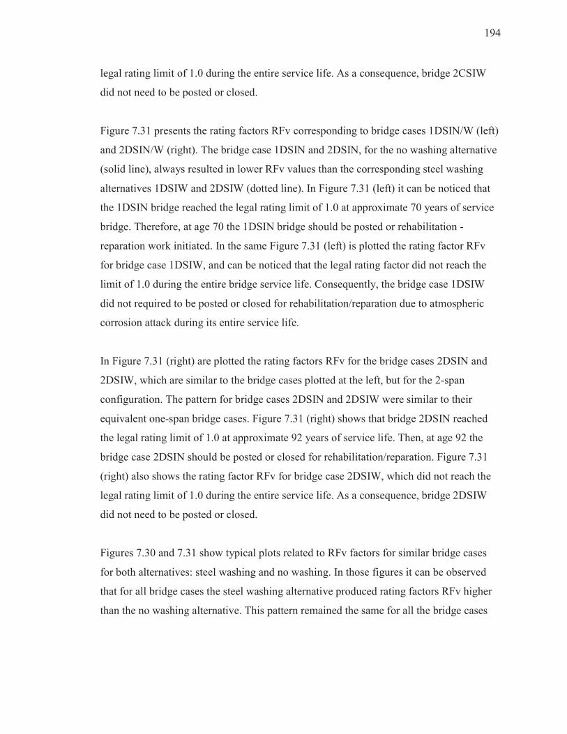
194
legal rating limit of 1.0 during the entire service life. As a consequence, bridge 2CSIW
did not need to be posted or closed.
Figure 7.31 presents the rating factors RFv corresponding to bridge cases 1DSIN/W (left)
and 2DSIN/W (right). The bridge case 1DSIN and 2DSIN, for the no washing alternative
(solid line), always resulted in lower RFv values than the corresponding steel washing
alternatives 1DSIW and 2DSIW (dotted line). In Figure 7.31 (left) it can be noticed that
the 1DSIN bridge reached the legal rating limit of 1.0 at approximate 70 years of service
bridge. Therefore, at age 70 the 1DSIN bridge should be posted or rehabilitation -
reparation work initiated. In the same Figure 7.31 (left) is plotted the rating factor RFv
for bridge case 1DSIW, and can be noticed that the legal rating factor did not reach the
limit of 1.0 during the entire bridge service life. Consequently, the bridge case 1DSIW
did not required to be posted or closed for rehabilitation/reparation due to atmospheric
corrosion attack during its entire service life.
In Figure 7.31 (right) are plotted the rating factors RFv for the bridge cases 2DSIN and
2DSIW, which are similar to the bridge cases plotted at the left, but for the 2-span
configuration. The pattern for bridge cases 2DSIN and 2DSIW were similar to their
equivalent one-span bridge cases. Figure 7.31 (right) shows that bridge 2DSIN reached
the legal rating limit of 1.0 at approximate 92 years of service life. Then, at age 92 the
bridge case 2DSIN should be posted or closed for rehabilitation/reparation. Figure 7.31
(right) also shows the rating factor RFv for bridge case 2DSIW, which did not reach the
legal rating limit of 1.0 during the entire service life. As a consequence, bridge 2DSIW
did not need to be posted or closed.
Figures 7.30 and 7.31 show typical plots related to RFv factors for similar bridge cases
for both alternatives: steel washing and no washing. In those figures it can be observed
that for all bridge cases the steel washing alternative produced rating factors RFv higher
than the no washing alternative. This pattern remained the same for all the bridge cases

195
considered in this study. Therefore, the steel washing alternative on steel highway bridges
reduces the rates on capacity degradation due to atmospheric corrosion attack.
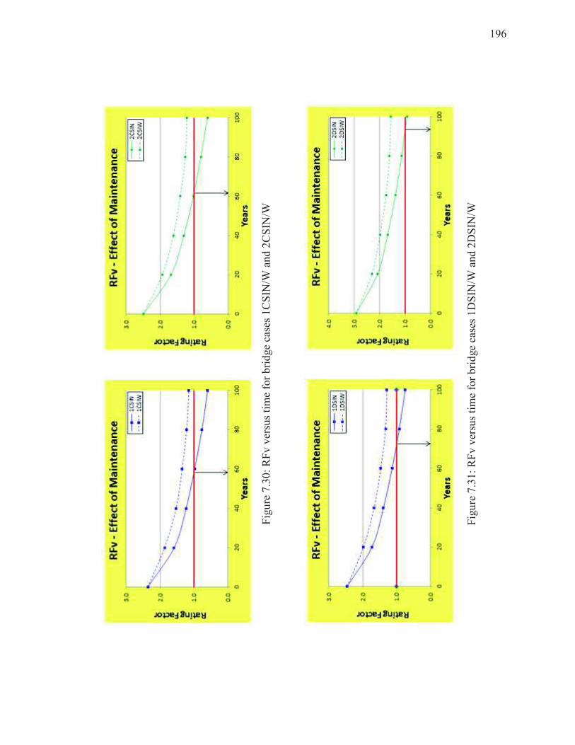
196
Fig
ure
7.3
0:
RF
v v
ersu
s ti
me
for
bri
dge
case
s 1
CS
IN/W
an
d 2
CS
IN/W
Fig
ure
7.3
1:
RF
v v
ersu
s ti
me
for
bri
dge
case
s 1
DS
IN/W
and
2D
SIN
/W

197
In this chapter have been analyzed the effects of all different variables considered in the
parametric study. It was analyzed the structural capacity degradation of steel girder
highway bridges due to atmospheric corrosion attack. The analyses considered both no
washing and steel bridge washing alternatives. The vast data acquired in this research
supports the statement that steel washing is an effective bridge maintenance activity,
reducing the structural capacity degradation of steel girder highway bridges. The steel
washing alternative resulted in a better option by reducing the rate of structural capacity
degradation when compared to the no washing option for all variables included in this
parametric study.

198
ECONOMIC EVALUATION OF CORRODED STEEL BRIDGES
8.1 Introduction
Economic evaluation of steel bridges is an analysis of future-value cash-flows,
representing all expenditures required to operate a bridge under the expected conditions
of serviceability. For the case of corroded steel bridges, the analysis should deal with
appropriate measures, and their respective costs, to control or fix the corrosion problem
with the aim of achieving the expected bridge service life.
“The cost of keeping a bridge in a safe and good condition is not a one-time expenditure
based on the initial cost of construction” (Bowman and Moran, 2015). The cost of
operating a bridge in good condition requires a long-term investment during the entire
expected service life (Hema et al., 2004). Due to normal exposure and operation, all
bridges experience a deterioration process. As a consequence, all bridge members
experience physical and mechanical changes over their service life, thereby resulting in a
decline in the bridge service condition and a corresponding reduction in structural
capacity (Abed-Al-Rahim and Johnston, 1995). One of the most dangerous changes for
steel bridge members is the loss of section due to corrosion attack. Knowledge of the
section loss rate of the steel bridge members is critical to reliably predict the bridge
service life.
To achieve the expected bridge service life, all elements of the structure should receive
appropriate maintenance, rehabilitation, and repairs, which can be provided applying
different strategies. The strategy selection is based on the transportation agencies’
expectations on bridge service life, the costs of possible strategies, and the available
199
resources to be used (Hawk, 2003). Bridge maintenance activities are performed based on
their effectiveness to reduce deterioration and according to the availability of enough
funds. DOT’s authorities are aware of the benefits of most strategic bridge maintenance
activities, and the convenient frequency to apply them.
Several studies have proved that scheduled preventive bridge maintenance activities are
more efficient and cost-effective than reactionary maintenance activities (NYSDOT,
2008; FHWA, 2011; Yanev, 2011). The expected benefit from performing bridge
maintenance activities is the service life extension, and as a consequence, delaying a
major bridge rehabilitation or even a bridge replacement. In order to select the best bridge
maintenance strategy among all available options, DOTs agencies are prone to use a cost-
benefit analysis, based on a Life-Cycle Cost Analysis.
8.2 Life Cycle Cost Analysis
Life-Cycle Cost Analysis (LCCA) is a decision making tool oriented to show the benefits
from different alternatives to achieve the same expected results (Azizinamini et al.,
2013). When performing a LCCA, cash flows from past, present or future interventions
must be evaluated and compared. A widely accepted method is evaluating the Present
Value (PV), which represents the value of any cash flow expressed as a value
corresponding to the present time. The LCCA procedure for bridge maintenance requires
the assumption of some values and factors, such as the costs of maintenance activities,
possible rehabilitation costs, bridge replacement cost, the expected bridge service life,
and the cost of funds expressed as a discount rate.
A LCCA is performed typically in the following sequential steps:
· Identify alternatives
· Define time for analysis, normally the bridge service life
· Define costs components for each alternative
· Evaluate PV for each alternative
200
· Compare PV from different alternatives and make a final decision
8.2.1 Bridge Service Life
Bridge service life is understood as the expected time span a bridge can perform properly
under the expected service conditions before major rehabilitation/replacement is required.
The bridge owner can implement several policies to pursue the expected bridge service
life. Those policies are based on the owner’s criteria, the knowledge of appropriate bridge
conservation measures, and most importantly, the available resources to implement the
selected measures to keep the bridge in good conditions over the entire service life. Most
of the references from specialized literature consider the bridge service life to be from 75
to 100 years (So, 2012; Azizinamini, 2013). In this research a bridge service life of 100
years was assumed for all analyses.
8.2.2 Cost of Bridge Maintenance Activities, Rehabilitation, and Replacement
The LCCA procedure requires several inputs to perform it appropriately. Cost of
alternatives to be compared are of the most essential, to achieve reliable results from a
LCCA. The main source to obtain accurate bridge maintenance, rehabilitation or
replacement costs is the historical data recorded for the maintenance unit of each agency.
There are several studies related to bridge maintenance activities. Some of those studies
provide unit costs for the most common bridge maintenance activities. Although, there
are few studies regarding bridge superstructure washing, and only very few of them
provide some data about unit costs.
Several unit costs related to bridge maintenance activities and major bridge rehabilitation
were collected and presented in the studies conducted by Sobanjo (2001) and Hearn
(2012). In this work were considered unit costs for steel bridge superstructure washing
and rehabilitate steel girder, as presented in Table 8.1.
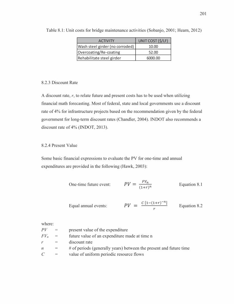
201
Table 8.1: Unit costs for bridge maintenance activities (Sobanjo, 2001; Hearn, 2012)
ACTIVITY UNIT COST ($/LF)
Wash steel girder (no corroded) 10.00
Overcoating/Re-coating 52.00
Rehabilitate steel girder 6000.00
8.2.3 Discount Rate
A discount rate, r, to relate future and present costs has to be used when utilizing
financial math forecasting. Most of federal, state and local governments use a discount
rate of 4% for infrastructure projects based on the recommendation given by the federal
government for long-term discount rates (Chandler, 2004). INDOT also recommends a
discount rate of 4% (INDOT, 2013).
8.2.4 Present Value
Some basic financial expressions to evaluate the PV for one-time and annual
expenditures are provided in the following (Hawk, 2003):
One-time future event: �� � ��
!"#$% Equation 8.1
Equal annual events: �� � & '"(!"#$%) *
$
Equation 8.2
where:
PV = present value of the expenditure
FVn = future value of an expenditure made at time n
r = discount rate
n = # of periods (generally years) between the present and future time
C = value of uniform periodic resource flows
202
Therefore, the benefit of considering certain maintenance activities can be determined by
comparing the PV of all the costs for the proposed maintenance activities against the PV
of the alternative that does not consider performing any maintenance activity. If the PV
of all the costs of the maintenance activities exceeds the PV of the alternative of not
performing any maintenance, then performing those maintenance activities may not be
worth pursuing and should likely be rejected. However, when the PV of the maintenance
activities is less than when no maintenance is performed, and sometimes far less than the
PV of the alternative of not performing maintenance, then the maintenance activities are
undoubtedly worth pursuing.
8.2.5 Bridge Load Rating
Bridge load rating was performed to determine the safe live load capacity that a bridge
can resist under the actual conditions of the structure. In Chapter 7 a parametric analysis
was applied to several composite steel girder highway bridge models, to determine the
live load capacity at three different levels: Inventory level, Operating level, and Legal
level. Each rating level has specific applications and consequences when the minimum
target is achieved. Inventory Level is the most demanding analysis, followed by
Operating level, and ending with the Legal level as the least demanding. The load rating
at those different levels were performed at different ages (0, 20, 40, 60, 80, and 100 years
of service) in order to determine the capacity degradation of the structure due to the
attack of atmospheric corrosion throughout the structure’s service life. The parametric
analysis also included wash/no-wash alternatives: either performing steel girder washing
as a maintenance activity or performing no steel girder washing.
The study of typical steel highway bridge models under those two alternatives
highlighted the effect of steel girder washing in reducing the rate of capacity degradation
under corrosion attack. The results showed in Chapter 7 support the statement that steel
girder washing is an effective bridge maintenance activity, to reduce atmospheric
corrosion, when performed regularly during the bridge service life.
203
Tables 8.2 show the ages, from the 96 bridge models considered in the evaluation, when
the bridge members reached their limits (RFv = 1.0) at any of the three rating levels.
Therefore, those bridge cases with no age shown in Tables 8.2 to 8.4 correspond to cases
in which the load rating limit of RFv = 1.00 was not reached for that specific load level
during the entire bridge service life.. Tables 8.2 to 8.4 show that a bridge under a steel
girder washing program always resulted in a less corroded situation than the same bridge
without girder washing.
Another source to understand the structural capacity degradation is relating the load
rating factor with the demand/capacity ratio of the structure. When a bridge case reaches
the limit rating factor of RFv = 1.00 at the Inventory level, the demand/capacity ratio for
shear is near to 1.00; when RFv = 1.0 at the Operating level, the demand/capacity ratio
for shear is near to 1.15; and when RFv = 1.0 at the Legal level, the demand/capacity
ratio for shear is close to 1.30. That means that the structure is overstressed by 15% when
reaching the load rating limit at Operating level, and overstressed by 30% at the limit for
load Legal level.
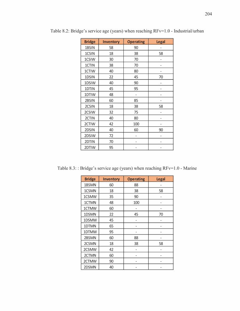
204
Table 8.2: Bridge’s service age (years) when reaching RFv=1.0 - Industrial/urban
Table 8.3: : Bridge’s service age (years) when reaching RFv=1.0 - Marine
Bridge Inventory Operating Legal
1BSIN 58 90 -
1CSIN 18 38 58
1CSIW 30 70 -
1CTIN 38 70 -
1CTIW 40 80 -
1DSIN 22 45 70
1DSIW 40 90 -
1DTIN 45 95 -
1DTIW 48 - -
2BSIN 60 85 -
2CSIN 18 38 58
2CSIW 32 75 -
2CTIN 40 80 -
2CTIW 42 100 -
2DSIN 40 60 90
2DSIW 72 - -
2DTIN 70 - -
2DTIW 95 - -
Bridge Inventory Operating Legal
1BSMN 60 88 -
1CSMN 18 38 58
1CSMW 35 90 -
1CTMN 48 100 -
1CTMW 60 - -
1DSMN 22 45 70
1DSMW 45 - -
1DTMN 65 - -
1DTMW 95 - -
2BSMN 60 88 -
2CSMN 18 38 58
2CSMW 42 - -
2CTMN 60 - -
2CTMW 90 - -
2DSMN 40 - -
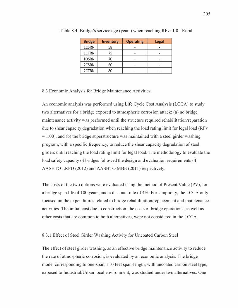
205
Table 8.4: Bridge’s service age (years) when reaching RFv=1.0 - Rural
8.3 Economic Analysis for Bridge Maintenance Activities
An economic analysis was performed using Life Cycle Cost Analysis (LCCA) to study
two alternatives for a bridge exposed to atmospheric corrosion attack: (a) no bridge
maintenance activity was performed until the structure required rehabilitation/reparation
due to shear capacity degradation when reaching the load rating limit for legal load (RFv
= 1.00), and (b) the bridge superstructure was maintained with a steel girder washing
program, with a specific frequency, to reduce the shear capacity degradation of steel
girders until reaching the load rating limit for legal load. The methodology to evaluate the
load safety capacity of bridges followed the design and evaluation requirements of
AASHTO LRFD (2012) and AASHTO MBE (2011) respectively.
The costs of the two options were evaluated using the method of Present Value (PV), for
a bridge span life of 100 years, and a discount rate of 4%. For simplicity, the LCCA only
focused on the expenditures related to bridge rehabilitation/replacement and maintenance
activities. The initial cost due to construction, the costs of bridge operations, as well as
other costs that are common to both alternatives, were not considered in the LCCA.
8.3.1 Effect of Steel Girder Washing Activity for Uncoated Carbon Steel
The effect of steel girder washing, as an effective bridge maintenance activity to reduce
the rate of atmospheric corrosion, is evaluated by an economic analysis. The bridge
model corresponding to one-span, 110 feet span-length, with uncoated carbon steel type,
exposed to Industrial/Urban local environment, was studied under two alternatives. One
Bridge Inventory Operating Legal
1CSRN 58 - -
1CTRN 75 - -
1DSRN 70 - -
2CSRN 60 - -
2CTRN 80 - -
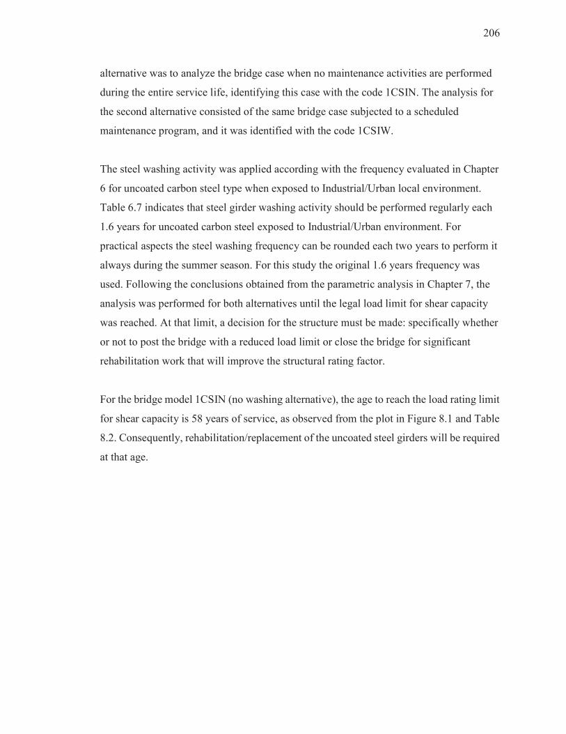
206
alternative was to analyze the bridge case when no maintenance activities are performed
during the entire service life, identifying this case with the code 1CSIN. The analysis for
the second alternative consisted of the same bridge case subjected to a scheduled
maintenance program, and it was identified with the code 1CSIW.
The steel washing activity was applied according with the frequency evaluated in Chapter
6 for uncoated carbon steel type when exposed to Industrial/Urban local environment.
Table 6.7 indicates that steel girder washing activity should be performed regularly each
1.6 years for uncoated carbon steel exposed to Industrial/Urban environment. For
practical aspects the steel washing frequency can be rounded each two years to perform it
always during the summer season. For this study the original 1.6 years frequency was
used. Following the conclusions obtained from the parametric analysis in Chapter 7, the
analysis was performed for both alternatives until the legal load limit for shear capacity
was reached. At that limit, a decision for the structure must be made: specifically whether
or not to post the bridge with a reduced load limit or close the bridge for significant
rehabilitation work that will improve the structural rating factor.
For the bridge model 1CSIN (no washing alternative), the age to reach the load rating limit
for shear capacity is 58 years of service, as observed from the plot in Figure 8.1 and Table
8.2. Consequently, rehabilitation/replacement of the uncoated steel girders will be required
at that age.
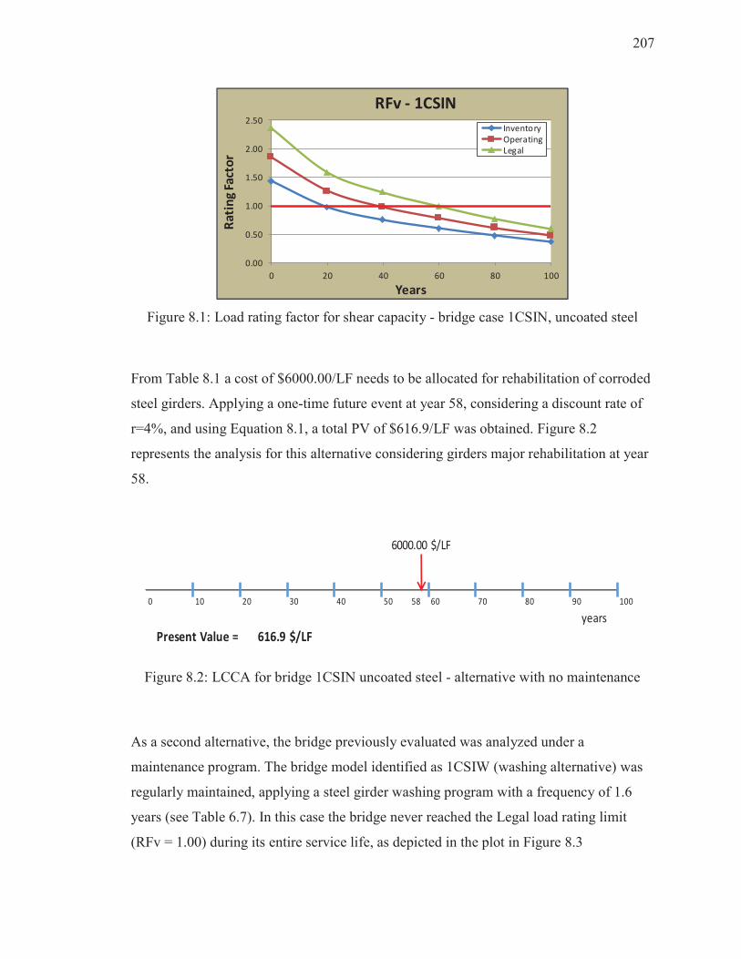
207
Figure 8.1: Load rating factor for shear capacity - bridge case 1CSIN, uncoated steel
From Table 8.1 a cost of $6000.00/LF needs to be allocated for rehabilitation of corroded
steel girders. Applying a one-time future event at year 58, considering a discount rate of
r=4%, and using Equation 8.1, a total PV of $616.9/LF was obtained. Figure 8.2
represents the analysis for this alternative considering girders major rehabilitation at year
58.
6000.00 $/LF
0 10 20 30 40 50 58 60 70 80 90 100
years
616.9 $/LFPresent Value =
Figure 8.2: LCCA for bridge 1CSIN uncoated steel - alternative with no maintenance
As a second alternative, the bridge previously evaluated was analyzed under a
maintenance program. The bridge model identified as 1CSIW (washing alternative) was
regularly maintained, applying a steel girder washing program with a frequency of 1.6
years (see Table 6.7). In this case the bridge never reached the Legal load rating limit
(RFv = 1.00) during its entire service life, as depicted in the plot in Figure 8.3
0.00
0.50
1.00
1.50
2.00
2.50
0 20 40 60 80 100
Ra
tin
g F
act
or
Years
RFv - 1CSIN
Inventory
Operating
Legal
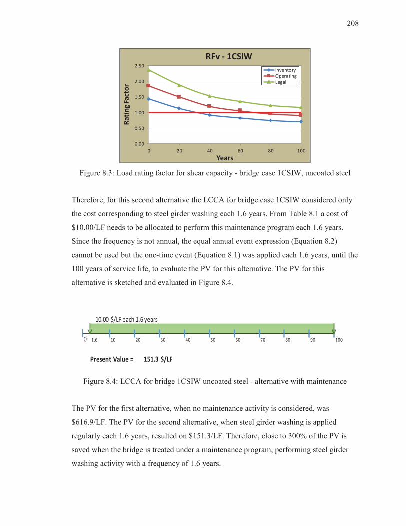
208
Figure 8.3: Load rating factor for shear capacity - bridge case 1CSIW, uncoated steel
Therefore, for this second alternative the LCCA for bridge case 1CSIW considered only
the cost corresponding to steel girder washing each 1.6 years. From Table 8.1 a cost of
$10.00/LF needs to be allocated to perform this maintenance program each 1.6 years.
Since the frequency is not annual, the equal annual event expression (Equation 8.2)
cannot be used but the one-time event (Equation 8.1) was applied each 1.6 years, until the
100 years of service life, to evaluate the PV for this alternative. The PV for this
alternative is sketched and evaluated in Figure 8.4.
Figure 8.4: LCCA for bridge 1CSIW uncoated steel - alternative with maintenance
The PV for the first alternative, when no maintenance activity is considered, was
$616.9/LF. The PV for the second alternative, when steel girder washing is applied
regularly each 1.6 years, resulted on $151.3/LF. Therefore, close to 300% of the PV is
saved when the bridge is treated under a maintenance program, performing steel girder
washing activity with a frequency of 1.6 years.
0.00
0.50
1.00
1.50
2.00
2.50
0 20 40 60 80 100
Ra
tin
g F
act
or
Years
RFv - 1CSIW
Inventory
Operating
Legal
10.00 $/LF each 1.6 years
0 1.6 10 20 30 40 50 60 70 80 90 100
151.3 $/LFPresent Value =
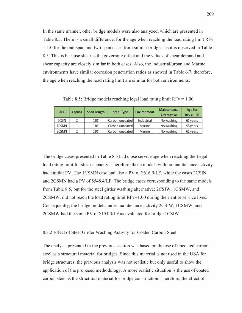
209
In the same manner, other bridge models were also analyzed, which are presented in
Table 8.5. There is a small difference, for the age when reaching the load rating limit RFv
= 1.0 for the one-span and two-span cases from similar bridges, as it is observed in Table
8.5. This is because shear is the governing effect and the values of shear demand and
shear capacity are closely similar in both cases. Also, the Industrial/urban and Marine
environments have similar corrosion penetration ratios as showed in Table 6.7, therefore,
the age when reaching the load rating limit are similar for both environments.
Table 8.5: Bridge models reaching legal load rating limit RFv = 1.00
2CSIN 2 110' Carbon uncoated Industrial No washing 61 years
1CSMN 1 110' Carbon uncoated Marine No washing 58 years
2CSMN 2 110' Carbon uncoated Marine No washing 61 years
BRIDGE # spans Span Length EnvironmentMaintenance
Alternative
Age for
RFv = 1.00Steel Type
The bridge cases presented in Table 8.5 had close service age when reaching the Legal
load rating limit for shear capacity. Therefore, those models with no maintenance activity
had similar PV. The 1CSMN case had also a PV of $616.9/LF, while the cases 2CSIN
and 2CSMN had a PV of $548.4/LF. The bridge cases corresponding to the same models
from Table 8.5, but for the steel girder washing alternative: 2CSIW, 1CSMW, and
2CSMW, did not reach the load rating limit RFv=1.00 during their entire service lives.
Consequently, the bridge models under maintenance activity 2CSIW, 1CSMW, and
2CSMW had the same PV of $151.3/LF as evaluated for bridge 1CSIW.
8.3.2 Effect of Steel Girder Washing Activity for Coated Carbon Steel
The analysis presented in the previous section was based on the use of uncoated carbon
steel as a structural material for bridges. Since this material is not used in the USA for
bridge structures, the previous analysis was not realistic but only useful to show the
application of the proposed methodology. A more realistic situation is the use of coated
carbon steel as the structural material for bridge construction. Therefore, the effect of
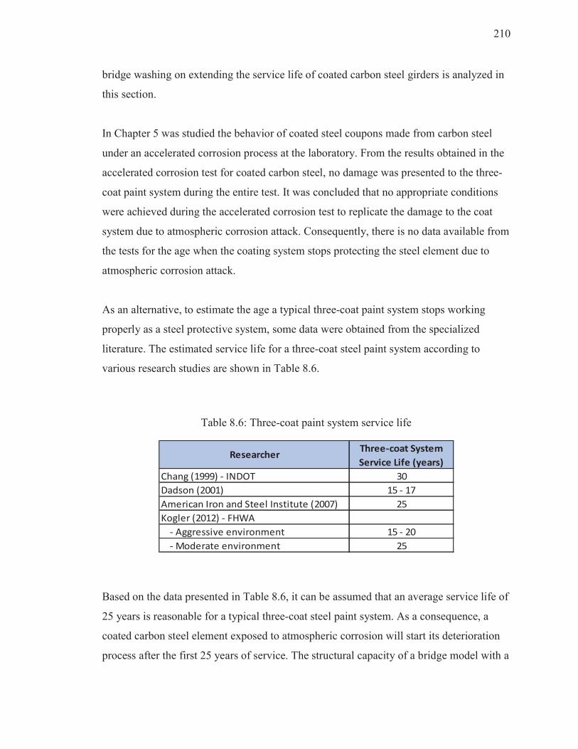
210
bridge washing on extending the service life of coated carbon steel girders is analyzed in
this section.
In Chapter 5 was studied the behavior of coated steel coupons made from carbon steel
under an accelerated corrosion process at the laboratory. From the results obtained in the
accelerated corrosion test for coated carbon steel, no damage was presented to the three-
coat paint system during the entire test. It was concluded that no appropriate conditions
were achieved during the accelerated corrosion test to replicate the damage to the coat
system due to atmospheric corrosion attack. Consequently, there is no data available from
the tests for the age when the coating system stops protecting the steel element due to
atmospheric corrosion attack.
As an alternative, to estimate the age a typical three-coat paint system stops working
properly as a steel protective system, some data were obtained from the specialized
literature. The estimated service life for a three-coat steel paint system according to
various research studies are shown in Table 8.6.
Table 8.6: Three-coat paint system service life
Based on the data presented in Table 8.6, it can be assumed that an average service life of
25 years is reasonable for a typical three-coat steel paint system. As a consequence, a
coated carbon steel element exposed to atmospheric corrosion will start its deterioration
process after the first 25 years of service. The structural capacity of a bridge model with a
Chang (1999) - INDOT 30
Dadson (2001) 15 - 17
American Iron and Steel Institute (2007) 25
Kogler (2012) - FHWA
- Aggressive environment 15 - 20
- Moderate environment 25
Three-coat System
Service Life (years)Researcher
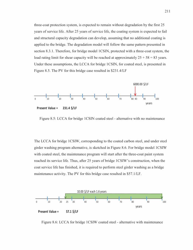
211
three-coat protection system, is expected to remain without degradation by the first 25
years of service life. After 25 years of service life, the coating system is expected to fail
and structural capacity degradation can develop, assuming that no additional coating is
applied to the bridge. The degradation model will follow the same pattern presented in
section 8.3.1. Therefore, for bridge model 1CSIN, protected with a three-coat system, the
load rating limit for shear capacity will be reached at approximately 25 + 58 = 83 years.
Under these assumptions, the LCCA for bridge 1CSIN, for coated steel, is presented in
Figure 8.5. The PV for this bridge case resulted in $231.4/LF
6000.00 $/LF
0 10 20 30 40 50 60 70 80 83 90 100
years
231.4 $/LFPresent Value =
Figure 8.5: LCCA for bridge 1CSIN coated steel - alternative with no maintenance
The LCCA for bridge 1CSIW, corresponding to the coated carbon steel, and under steel
girder washing program alternative, is sketched in Figure 8.6. For bridge model 1CSIW
with coated steel, the maintenance program will start after the three-coat paint system
reached its service life. Thus, after 25 years of bridge 1CSIW’s construction, when the
coat service life has finished, it is required to perform steel girder washing as a bridge
maintenance activity. The PV for this bridge case resulted in $57.1/LF.
Figure 8.6: LCCA for bridge 1CSIW coated steel - alternative with maintenance
10.00 $/LF each 1.6 years
0 10 20 25 30 40 50 60 70 80 90 100
years
$/LF57.1Present Value =

212
For bridge case 1CSIN made from coated steel, corresponding to the no maintenance
alternative, its PV resulted on $231.4/LF. For the bridge case 1CSIW made from coated
steel, when steel girder washing is applied regularly each 1.6 years, resulted on a PV of
$57.1/LF. Therefore, close to 300% of the PV is saved when the coated steel girder
highway bridge is treated under a maintenance program, performing steel girder washing
activity with a frequency of 1.6 years, starting the program at age 25 of service life.
Following the same procedure presented in Section 8.3.1, the bridge models presented in
Table 8.5 (2CSIN, 1CSMN, 2CSMN) but made from coated carbon steel, were analyzed
until the Legal load rating limit for shear capacity was reached. The bridge case 1CSMN,
with protection coating system, had a similar service life of 83 years as bridge 1CSIN
case, and also a PV of $231.4/LF. Bridge cases 2CSIN and 2CSMN, with protection
coating system, had service life of approximately 25 + 61 = 86 years and a PV of
$205.7/LF. At the other hand, the three cases (2CSIW, 1CSMW, 2CSMW) subjected to a
maintenance program of steel girder washing performed each 1.6 years and starting after
the first 25 years of service life (after the coating system has deteriorated) did not reach
the load rating limit RFv = 1.0 during their entire service life, having all of them a PV of
$57.1/LF.
In Table 8.7 are summarized the results for the bridge cases analyzed, for uncoated and
coated carbon steel, with and without steel girder washing as a regular maintenance
program. The no maintenance program included a steel girder rehabilitation of
deteriorated girders after reaching their service life. The maintenance program consisted
in regular steel girder washing each 1.6 years, starting at year zero for uncoated girders
and after the first 25 years of service life for coated girders. As presented in Table 8.5, the
bridge cases under maintenance program reached the 100 years of service life without
rehabilitation/replacement.
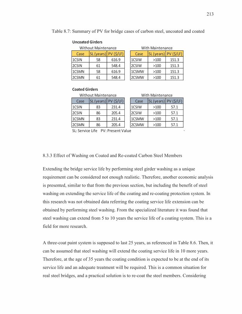
213
Table 8.7: Summary of PV for bridge cases of carbon steel, uncoated and coated
Case SL (years) PV ($/LF) Case SL (years) PV ($/LF)
1CSIN 58 616.9 1CSIW >100 151.3
2CSIN 61 548.4 2CSIW >100 151.3
1CSMN 58 616.9 1CSMW >100 151.3
2CSMN 61 548.4 2CSMW >100 151.3
Case SL (years) PV ($/LF) Case SL (years) PV ($/LF)
1CSIN 83 231.4 1CSIW >100 57.1
2CSIN 86 205.4 2CSIW >100 57.1
1CSMN 83 231.4 1CSMW >100 57.1
2CSMN 86 205.4 2CSMW >100 57.1
SL: Service Life PV: Present Value
Without Maintenance With Maintenance
Without Maintenance With Maintenance
Uncoated Girders
Coated Girders
`
8.3.3 Effect of Washing on Coated and Re-coated Carbon Steel Members
Extending the bridge service life by performing steel girder washing as a unique
requirement can be considered not enough realistic. Therefore, another economic analysis
is presented, similar to that from the previous section, but including the benefit of steel
washing on extending the service life of the coating and re-coating protection system. In
this research was not obtained data referring the coating service life extension can be
obtained by performing steel washing. From the specialized literature it was found that
steel washing can extend from 5 to 10 years the service life of a coating system. This is a
field for more research.
A three-coat paint system is supposed to last 25 years, as referenced in Table 8.6. Then, it
can be assumed that steel washing will extend the coating service life in 10 more years.
Therefore, at the age of 35 years the coating condition is expected to be at the end of its
service life and an adequate treatment will be required. This is a common situation for
real steel bridges, and a practical solution is to re-coat the steel members. Considering
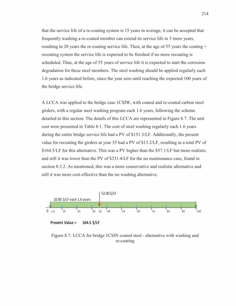
214
that the service life of a re-coating system is 15 years in average, it can be accepted that
frequently washing a re-coated member can extend its service life in 5 more years,
resulting in 20 years the re-coating service life. Then, at the age of 55 years the coating +
recoating system the service life is expected to be finished if no more recoating is
scheduled. Thus, at the age of 55 years of service life it is expected to start the corrosion
degradation for these steel members. The steel washing should be applied regularly each
1.6 years as indicated before, since the year zero until reaching the expected 100 years of
the bridge service life.
A LCCA was applied to the bridge case 1CSIW, with coated and re-coated carbon steel
girders, with a regular steel washing program each 1.6 years, following the scheme
detailed in this section. The details of this LCCA are represented in Figure 8.7. The unit
cost were presented in Table 8.1. The cost of steel washing regularly each 1.6 years
during the entire bridge service life had a PV of $151.3/LF. Additionally, the present
value for recoating the girders at year 35 had a PV of $13.2/LF, resulting in a total PV of
$164.5/LF for this alternative. This was a PV higher than the $57.1/LF but more realistic
and still it was lower than the PV of $231.4/LF for the no maintenance case, found in
section 8.3.2. As mentioned, this was a more conservative and realistic alternative and
still it was more cost-effective than the no washing alternative.
10.00 $/LF each 1.6 years
0 1.6 10 20 30 35 40 50 60 70 80 90 100
164.5 $/LFPresent Value =
52.00 $/LF
Figure 8.7: LCCA for bridge 1CSIN coated steel - alternative with washing and re-coating
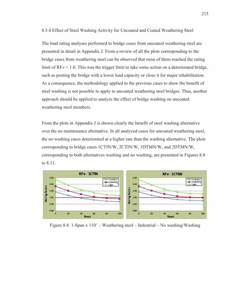
215
8.3.4 Effect of Steel Washing Activity for Uncoated and Coated Weathering Steel
The load rating analyses performed to bridge cases from uncoated weathering steel are
presented in detail in Appendix J. From a review of all the plots corresponding to the
bridge cases from weathering steel can be observed that none of them reached the rating
limit of RFv = 1.0. This was the trigger limit to take some action on a deteriorated bridge,
such as posting the bridge with a lower load capacity or close it for major rehabilitation.
As a consequence, the methodology applied to the previous cases to show the benefit of
steel washing is not possible to apply to uncoated weathering steel bridges. Thus, another
approach should be applied to analyze the effect of bridge washing on uncoated
weathering steel members.
From the plots in Appendix J is shown clearly the benefit of steel washing alternative
over the no maintenance alternative. In all analyzed cases for uncoated weathering steel,
the no washing cases deteriorated at a higher rate than the washing alternative. The plots
corresponding to bridge cases 1CTIN/W, 2CTIN/W, 1DTMN/W, and 2DTMN/W,
corresponding to both alternatives washing and no washing, are presented in Figures 8.8
to 8.11.
Figure 8.8: 1-Span x 110’ – Weathering steel – Industrial – No washing/Washing
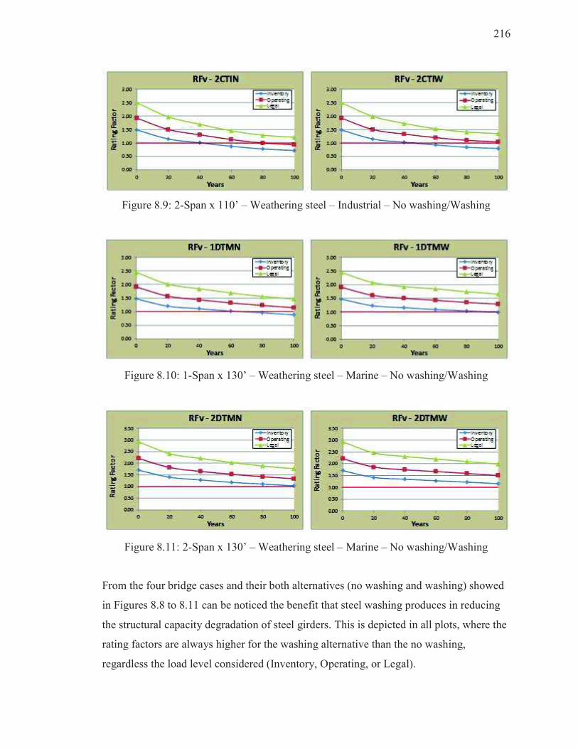
216
Figure 8.9: 2-Span x 110’ – Weathering steel – Industrial – No washing/Washing
Figure 8.10: 1-Span x 130’ – Weathering steel – Marine – No washing/Washing
Figure 8.11: 2-Span x 130’ – Weathering steel – Marine – No washing/Washing
From the four bridge cases and their both alternatives (no washing and washing) showed
in Figures 8.8 to 8.11 can be noticed the benefit that steel washing produces in reducing
the structural capacity degradation of steel girders. This is depicted in all plots, where the
rating factors are always higher for the washing alternative than the no washing,
regardless the load level considered (Inventory, Operating, or Legal).

217
Additionally, when considering a bridge case from coated weathering steel, the same
criteria from section 8.3.3 can be followed. In section 8.3.3 it was assumed that washing
carbon steel girders protected with an initial coat and recoated after 35 years is more cost-
effective than the no washing alternative. Hence, it can be considered that the coating
system for weathering steel will have the same service life of 35 years that had the coat
for a carbon steel member. Also, it can be accepted that a re-coating system for
weathering steel will last the same 20 years it lasted for a carbon steel member.
Therefore, after 55 years of service life, the coating system of a weathering steel member
will be ended and structural deterioration will develop. Then, maintaining under a regular
washing program a weathering steel member, initially coated and recoated only once
after 35 years of service life, will allow it to reach its service life with lower capacity
degradation than the no washing alternative. When exposed to Industrial/urban
environment, weathering steel should be washed regularly each 3.8 years, as found in
section 6.3.2 and presented in Table 6.8.
8.4 Results from LCCA
From the PV obtained for the bridge cases considered herein, it can be concluded that
periodic washing of steel highway bridge girders is a cost-effective bridge maintenance
option to reduce the structural capacity degradation due to atmospheric corrosion. The
conclusions are valid for bridges made from uncoated and coated carbon and weathering
steel.
The presented analyses focused on those bridges that reached the load rating limit for
shear capacity when submitted to Legal loads during their service lives. The analysis for
Legal load level is the less demanding condition, as prescribed by the AASHTO MBE
(2011). Therefore, for a more demanding condition, the load rating limit will be reached
at an early age, and consequently the Present Value (PV) will be higher than those
estimated for Legal loads.

218
The unit costs considered in this research were obtained from a specialized source, but
always those values are accepted with precaution. Special attention should be given to
rehabilitation/replacement costs, which actually reflects the bridge owner costs with some
approximation. Rehabilitation and replacement and major works unit costs do not reflect
the user costs, which are quite specific for each case, difficult to estimate, and often are
not considered. Consequently, the rehabilitation/replacement activities could represent
higher costs than those reflected by unit cost found in the specialized literature.
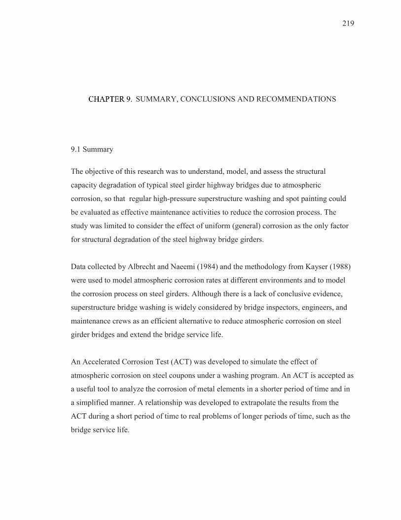
219
SUMMARY, CONCLUSIONS AND RECOMMENDATIONS
9.1 Summary
The objective of this research was to understand, model, and assess the structural
capacity degradation of typical steel girder highway bridges due to atmospheric
corrosion, so that regular high-pressure superstructure washing and spot painting could
be evaluated as effective maintenance activities to reduce the corrosion process. The
study was limited to consider the effect of uniform (general) corrosion as the only factor
for structural degradation of the steel highway bridge girders.
Data collected by Albrecht and Naeemi (1984) and the methodology from Kayser (1988)
were used to model atmospheric corrosion rates at different environments and to model
the corrosion process on steel girders. Although there is a lack of conclusive evidence,
superstructure bridge washing is widely considered by bridge inspectors, engineers, and
maintenance crews as an efficient alternative to reduce atmospheric corrosion on steel
girder bridges and extend the bridge service life.
An Accelerated Corrosion Test (ACT) was developed to simulate the effect of
atmospheric corrosion on steel coupons under a washing program. An ACT is accepted as
a useful tool to analyze the corrosion of metal elements in a shorter period of time and in
a simplified manner. A relationship was developed to extrapolate the results from the
ACT during a short period of time to real problems of longer periods of time, such as the
bridge service life.
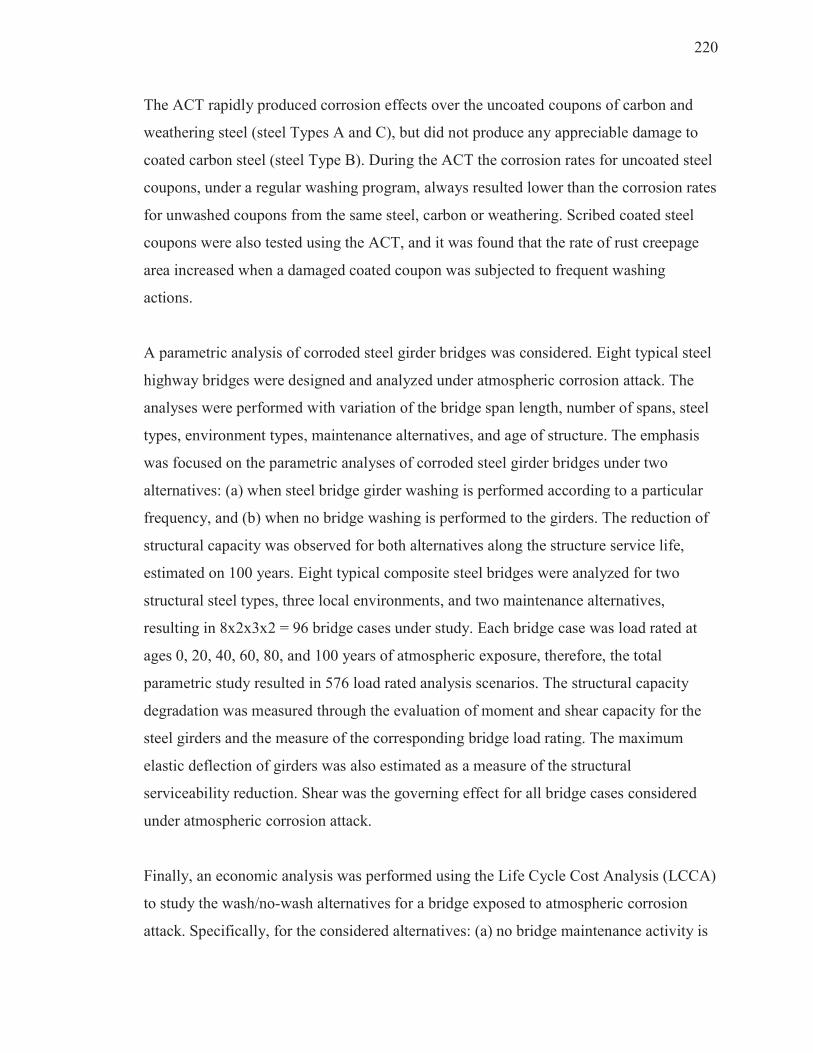
220
The ACT rapidly produced corrosion effects over the uncoated coupons of carbon and
weathering steel (steel Types A and C), but did not produce any appreciable damage to
coated carbon steel (steel Type B). During the ACT the corrosion rates for uncoated steel
coupons, under a regular washing program, always resulted lower than the corrosion rates
for unwashed coupons from the same steel, carbon or weathering. Scribed coated steel
coupons were also tested using the ACT, and it was found that the rate of rust creepage
area increased when a damaged coated coupon was subjected to frequent washing
actions.
A parametric analysis of corroded steel girder bridges was considered. Eight typical steel
highway bridges were designed and analyzed under atmospheric corrosion attack. The
analyses were performed with variation of the bridge span length, number of spans, steel
types, environment types, maintenance alternatives, and age of structure. The emphasis
was focused on the parametric analyses of corroded steel girder bridges under two
alternatives: (a) when steel bridge girder washing is performed according to a particular
frequency, and (b) when no bridge washing is performed to the girders. The reduction of
structural capacity was observed for both alternatives along the structure service life,
estimated on 100 years. Eight typical composite steel bridges were analyzed for two
structural steel types, three local environments, and two maintenance alternatives,
resulting in 8x2x3x2 = 96 bridge cases under study. Each bridge case was load rated at
ages 0, 20, 40, 60, 80, and 100 years of atmospheric exposure, therefore, the total
parametric study resulted in 576 load rated analysis scenarios. The structural capacity
degradation was measured through the evaluation of moment and shear capacity for the
steel girders and the measure of the corresponding bridge load rating. The maximum
elastic deflection of girders was also estimated as a measure of the structural
serviceability reduction. Shear was the governing effect for all bridge cases considered
under atmospheric corrosion attack.
Finally, an economic analysis was performed using the Life Cycle Cost Analysis (LCCA)
to study the wash/no-wash alternatives for a bridge exposed to atmospheric corrosion
attack. Specifically, for the considered alternatives: (a) no bridge maintenance activity is
221
performed until the bridge structure required rehabilitation/reparation due to shear
capacity degradation, when reaching the load rating limit for legal load (RFv = 1.00); and
(b) when the bridge superstructure was maintained with a steel girder washing program,
with a specific frequency, to reduce the shear capacity degradation of steel girders until
reaching the load rating limit for legal load.
9.2 Conclusions
Bridges are fundamental elements of a highway system, representing an important
investment and a strategic link that facilitates the transport of persons and goods. The
cost to rehabilitate or replace a highway bridge represents an important, and often
significant, expenditure for the owner, who needs to evaluate the correct time to assume
that cost. Consequently, prolonging the service lives of highway bridges by requiring
only short interruptions is an effective way to provide optimal service for the users and to
make more efficient use of the owner’s scarce resources.
An ACT following the ASTM B117 standard test resulted in an effective procedure to
reproduce atmospheric corrosion on small uncoated steel coupons in a shorter period of
time and in a simplified manner. The implemented ACT failed to reproduce atmospheric
corrosion on coated steel coupons, probably due to the absence of UV light emission
during the test, which can lead to the deterioration in the effectiveness of the coating
materials.
From the ACT implemented in this research, uncoated steel coupons from carbon and
weathering steel, regularly washed, presented lower rates of corrosion than the coupons
that were not washed. Based upon a correlation developed between corrosion initiated
using the ACT and corrosion for actual in-situ environments, different curves were
constructed to estimate corrosion penetration for each type of uncoated steel, and for each
local environment, versus the service age of the steel bridge. In all these curves, the steel
washing alternative provided lower corrosion rates than the no washing alternative. As
expected, corrosion rates were found larger for carbon steel than for weathering steel.
222
Correlation between the ACT and corrosion penetration at real environments was used to
determine the optimum average frequency a steel girder bridge should be washed. It was
found that uncoated carbon steel girders should be washed each 1.6, 1.7, and 5.7 years,
when exposed to Industrial/Urban, Marine, and Rural environments, respectively.
Uncoated weathering steel girders should be washed each 3.8, 6.0, and 10.9 years, when
exposed to Industrial/Urban, Marine, and Rural environments, respectively.
It was found from the parametric structural analysis of the 96 typical steel bridges, for the
six different service ages along the 100-years structure service life, that the steel washing
alternative reduces the rates of capacity degradation due to atmospheric corrosion,
regardless of the:
· type of stress - bending or shear.
· local environment - Industrial/Urban, Marine, or Rural.
· number of bridge spans - one or two.
· span length - 70, 90, 110, or 130 feet.
· steel type -uncoated carbon steel or uncoated weathering steel.
It was also observed that the steel washing alternatives always produced lower live-load
deflections than the no washing alternatives. This observation confirms that the steel
washing alternative reduces the structural capacity degradation on steel girder bridges
due to atmospheric corrosion attack.
Some differences were found for corrosion penetration rates from two sources, the
Control Test coupons and Group 10 coupons. Due to the several factors affecting the
accelerated corrosion test procedure, it was decided to proceed the structural capacity
analysis using data from Control Test. The selected data for corrosion rates provided a
more conservative analysis, since the higher corrosion rates were employed. A more deep
analysis can be performed using the complete original data presented in the
corresponding appendices.
223
The parametric load rating analysis showed that the bridge shear capacity was reduced at
a higher rate than the bending capacity. The structural capacity was measured through the
rating factors for bending (RFm) and shear (RFv). As a result, the shear rating limit of
RFv = 1.00 was reached at early ages than the bending rating limit of RFm = 1.0 in all
bridge cases. The reason for this behavior is believed to be the result of corrosion on both
faces of the web, making it a critical slender element, since the girder shear capacity is
provided entirely by the web section. The load rating analysis also confirmed that steel
girder washing is an effective maintenance alternative to reduce the atmospheric
corrosion attack, in comparison to the no washing alternative.
The economic analysis, using the LCCA method, also demonstrated that it is more cost-
effective to perform steel girder washing as a scheduled maintenance activity in contrast
to the no washing alternative for uncoated or coated carbon steel. The no-washing case
typically resulted in reaching the Legal load rating limit of RFv = 1.00 sooner during
their service lives than for cases with regular bridge washing, and consequently they had
to be closed sooner for girder rehabilitation/replacement. The economic evaluation for a
closed bridge for girder rehabilitation/replacement resulted in a Present Value (PV)
higher than the PV corresponding to the alternative when the bridge is maintained using a
regular steel girder washing program. For uncoated and coated weathering steel the
benefit of a regular washing program was determined by the analysis of structural
capacity degradation. The structural capacity degradation was measured by the load
rating factor for shear capacity RFv, which always resulted higher for the washing
alternative than the no washing.
The structural capacity degradation considered in this research was based only on the
atmospheric corrosion attack. Therefore, some other negative effects from natural or
human origin that can cause deterioration of steel highway bridge girders were not
considered in this study. The models created for corrosion penetration, and for corrosion
propagation in the girder section, should be considered as a rough approximation to
actual behavior on steel girder bridges.
224
Coated steel girders with spot damages should be repaired applying spot painting as soon
as possible. It is recommended to follow recommendations from the paint producer. The
damaged spot must be cleaned properly before painting application.
Performing steel washing on spot damages was found counterproductive, according to
results obtained in this research. Therefore, the solution for this type of problems is not
washing but spot painting as soon as possible.
In general, Industrial/urban and marine environments were always more aggressive than
rural environment. For rural environment the analyzed bridge cases never reached the
load rating limit of RFv = 1.0. For Industrial/urban and Marine environments, some
bridge cases did not reach the load rating limit of RFv = 1.0 due to their larger initial
structural capacity than those that reached the rating limit.
Based on the models assumed in this research, under the limited data available for the
estimation of actual atmospheric corrosion rates, accepting the several assumptions
proposed throughout the study, and following the methodology proposed herein, it was
found that regular, periodic washing of the steel highway bridge girders resulted in an
effective bridge maintenance activity that extended the service life of the girders. The
results from this research showed that steel girder washing reduced the rate of shear
structural capacity degradation of steel highway bridges exposed to atmospheric
corrosion attack in comparison to the alternative of not washing the steel girders.
9.3 Recommendations
Further research on corrosion penetration under actual environmental conditions would
be useful. The corrosion models used in this research are based on data obtained from
some particular locations, and consequently, a generalization of those results to be
applied in any other location will include some type of deviation and uncertainty. Also,
the limitations of the accelerated corrosion testing should be explored further to address
more realistic modeling of the actual environment.
225
Data from actual steel girder bridges should be recorded with an appropriate
methodology, following the same protocols at different agencies. Special consideration
should be given to the record of: corrosion penetration rates on steel girders at different
ages of service, unit costs of steel girder washing, steel girder washing procedures, and
how frequent is performed the steel girder washing.
The methodology presented should be improved in order to evaluate more precisely the
effectiveness of steel girder washing as a preventive maintenance activity and determine
the adequate frequency of washing. This methodology could be considered as a better
alternative, over the informal and intuitive procedures currently used, to decide the
implementation of this maintenance activity.
Appropriate procedures at the laboratory should be developed to study the effect of
atmospheric corrosion on coated steel elements and the benefit of regular steel washing
as an effective maintenance activity to reduce the corrosion rates.

LIST OF REFERENCES
226
LIST OF REFERENCES
AASHTO (2011). “The Manual for Bridge Evaluation.” American Association of State
Highway and Transportation Officials. AASHTO (2012). “AASHTO LRFD Bridge Design Specifications.” American
Association of State Highway and Transportation Officials. Abed-Al-Rahim, I., Johnston, D., (1995). “Bridge Element Deterioration Rates.”
Transportation Research Record 1490. TRB, National Research Council, Washington, D.C.,
AISC, (2015). “About the Steel Day Facility Tours: Steel Mills.” American Institute of
Steel Construction. Steelday. https://www.aisc.org/content.aspx?id=23272 [Accessed January 16, 2015]
AISI (1985). Steel Product Manual—Plates, American Iron and Steel Institute,
Washington, DC. Albrecht, P. and Naeemi, A. (1984). “Performance of Weathering Steel in Bridges.”
National Cooperative Highway Research Program. NCHRP Report 272. Transportation Research Board
Albrecht, P., Hall, T., (2003). “Atmospheric Corrosion Resistance of Structural Steels.”
American Society of Civil Engineers. Journal of Materials in Civil Engineering. Vol. 15, No. 1.
Appleman, B., Weaver, R., Bruno, J., (1995). “Maintenance Coating of Weathering Steel:
Field Evaluation and Guidelines.” Research and Development, Turner-Fairbank Highway Research Center. Report No. FHWA-RD-92-055.
ASTM (2008). “ASTM D1654-08 - Standard Test Method for Evaluation of Painted or
Coated Specimens Subjected to Corrosive Environments.” American Society for Testing and Materials
227
ASTM (2010). “ASTM D7087-05a (2010) - Standard Test Method for an Imaging Technique to Measure Rust Creepage at Scribe on Coated Test Panels Subjected to Corrosive Environments.” American Society for Testing and MaterialsASTM (2011). “ASTM B117-11 - Standard Practice for Operating Salt Spray (Fog) Apparatus.” American Society for Testing and Materials
ASTM (2011). “ASTM G1-03 (2011) - Standard Practice for Preparing, Cleaning, and
Evaluating Corrosion Test Specimens.” American Society for Testing and Materials ASTM, (2012). “ASTM D610-08 (2012) - Standard Practice for Evaluating Degree of
Rusting on Painted Steel Surfaces.” American Society for Testing and Materials AutoCAD 2016 (2016). “Autodesk Inc.”
Azizinamini, A., Power, E., Meyers, G., Ozyildirim, H., Kline, E., Whitmore, D., and
Mertz, D., (2013). “Design Guide for Bridges for Service Life.” Strategic Highway
Research Program, Transportation Research Board, SHRP 2 Renewal Project R19A.
Barker, R., and Puckett, J., (2007). “Design of Highway Bridges – An LRFD Approach.”
John Wiley & Sons, Inc. Barth, K., (2012). “Steel Bridge Design Handbook. Design Example 2A: Two-Span
Continuous Straight Composite Steel I-Girder Bridge.” Office of Bridge Technology Federal Highway Administration. Publication No. FHWA-IF-12-052 - Vol. 21.
Berman, J., Roeder, C., Burgdorfer, R., (2013). “Determining the Cost/Benefit of Routine
Maintenance Cleaning on Steel Bridges to Prevent Structural Deterioration.” Washington State Department of Transportation. WSDOT Research Report. Report No. WA-RD-11.1
Bowman, M., and Moran, L., (2015). “Bridge Preservation Treatments and Best
Practices.” Joint Transportation Research Program. SPR-3617. Purdue University,
Indiana Department of Transportation, USDOT, FHWA.
Bradford, S., (1998). “Practical Self-Study Guide to Corrosion Control.” CASTI
Publishing Inc. Caltrans, (2015). “Bridge Design Practice – Chapter 9: Steel Plate Girders”
http://www.dot.ca.gov/des/techpubs/manuals/bridge-design-practice/page/bdp-9.pdf [Accessed January 16, 2015]
Cambier, S., (2014). “Atmospheric Corrosion of Coated Steel; Relationship between
Laboratory and Field Testing.” PhD Dissertation in Civil Engineering. Ohio State University.
228
Carlsson, B., Engstrom, G., Lejre, A., Johansson, M., Lahtinen, R., Strom, M., (2006). “Guideline for Selection of Accelerated Corrosion Test for Product Qualification.” Nordic Innovation Centre. NORDTEST Technical Report TR-597.
Chandler, R., (2004). “Life-Cycle Cost Model for Evaluating the Sustainability of Bridge
Decks.” Center for Sustainable Systems. University of Michigan. Report No. CSS04-06.
Chang, L.-M., Zayed, T., Fricker, J. (1999). “Steel bridge protection policy – Volume IV:
Life cycle cost analysis and maintenance plan.” FHWA/IN/JTRP-98/21, Purdue
University, Indiana Department of Transportation, USDOT, FHWA.
Chong, S., and Yao, Y., (2007). “Selecting Overcoats for Bridges.” Public Roads.
Publication No. FHWA-HRT-07-006. Issue No. Vol. 71, No. 2 Computers & Structures, Inc., (2011). “CSiBridge v15 - Bridge Superstructure Design.”
Computers & Structures, Inc. Structural and Earthquake Engineering Software. Corus Construction Center. “Corrosion Protection of Steel Bridges.” Corus Construction
Center. Brochure (2002). Crampton, D., Holloway, K., Fraczek, J., (2013). “Assessment of Weathering Steel
Bridge Performance in Iowa and Development of Inspection and Maintenance Techniques.” Wiss, Janney, Elstner Associates, Inc. Final Report SPR 90-00-RB17-012. WJE No. 2011.1671
Cremer, (1996). “The Move to Cyclic Salt Spray Testing from Continuous Salt Spray.”
Anti-Corrosion Methods and Materials. Volume 43 – Number 3. Czarnecki, A., (2006). “System reliability Models for Evaluation of Corroded Steel
Girder Bridges.” PhD Dissertation in Civil Engineering. University of Michigan. Drazic, D., Vascic, V. (1989). “The Correlation between Accelerated Laboratory
Corrosion Tests and Atmospheric Corrosion Station Tests on Steels.” Corrosion Science, Vol. 29, No. 10,
Eom, J., (2014). “Reliability Analysis Model for Deflection Limit State of Deteriorated
Steel Girder Bridges.” Journal of the Korea Institute for Structural Maintenance and Inspection Vol. 18, No. 2, March 2014.
FHWA, (1989). “Uncoated Weathering Steel in Structures.” Technical Advisory 5140.22.
https://www.fhwa.dot.gov/bridge/t514022.cfm [Accessed Jan. 16, 2015].
229
FHWA, (2011). “Bridge Preservation Guide – Maintaining a State of Good Repair Using Cost Effective Investment Strategies.” FHWA Publication Number: FHWA-HIF-11042.
FHWA, (2012). “Steel Bridge Design Handbook.” US Department of Transportation. FHWA, (2015). USDOT. “Bridges and Structures – Bridges by Year Built 2013”. Federal
Highway Administration. US. Department of Transportation. http://www.fhwa.dot.gov/bridge/structyr.cfm [Accessed Jan. 16, 2015].
Fontana, M., (1986). “Corrosion Engineering.” McGraw-Hill Book Company. Ford, K., Arman, M., Labi, S., Sinha, K., Thompson, P., Shirole, A., Li, Z., (2012).
“Estimating Life Expectancies of Highway Assets – Volume 2: Final Report.” National Cooperative Highway Research Program. NCHRP Report 713. Transportation Research Board.
Golabi, K., Thompson, P., Hyman, W., (1993). “Pontis Technical Manual.” Technical
Report No. FHWA-SA-94-031. Optima Inc. and Cambridge Systematics, Inc. Guthrie, J., Battat, B., Grethlein, C., (2002). “Accelerated Corrosion Test.” The
AMPTIAC Quarterly, Volume 6, Number 3 11. Hara, S., Miura, M., Uchiumi, Y., Fujiwara, T., Yamamoto, M., (2005). “Suppression of
Deicing Salt Corrosion of Weathering Steel Bridges by Washing.” Corrosion Science 47.
Hawk, H. (2003). “Bridge Life-Cycle Cost Analysis.” National Cooperative Highway
Research Program. NCHRP Report 483. Transportation Research Board. Hearn, G., (2012). “Deterioration and Cost Information for Bridge Management.”
Colorado Department of Transportation. DTD Applied Research and Innovation Branch. Report No. CDOT-2012-4. Final Report.
Hema, J., Guthrie, W., Fonseca, F., (2004). “Concrete Bridge Deck Condition
Assessment and Improvement Strategies.” Utah Department of Transportation. Report UT-04-16
Hopwood, T. and Meade, B., (1999). “Experimental Maintenance Painting by
Overcoating on the I-64, I-71 and KY-22 Bridges.” Research Report KTC-99-51. Kentucky Transportation Center. College of Engineering, University of Kentucky. Kentucky Transportation Cabinet.
INDOT (2012). “Standard Specifications.” Indiana Department of Transportation.

230
INDOT (2013). “Design Manual.” Indiana Department of Transportation. ITD, (2008). “Bridge Design LRFD Manual.” Idaho Transportation Department Itoh, Y., Iwata, A., Kainuma, S., Kadota, Y., Kitagawa, T., (2006). “Accelerated
Exposure Tests of Durability for Steel Bridges.” Center for Integrated Research in Science and Engineering, Nagoya University, Japan
Jones, D., (1996). “Principles and Prevention of Corrosion.” Prentice Hall, Inc. Kayser, J. and Nowak, A., (1989). “Reliability of Corroded Steel Girder Bridges.”
Structural Safety, 6. Kayser, J., (1988). “The Effects of Corrosion on the Reliability of Steel Girder Bridges.”
PhD Dissertation in Civil Engineering. University of Michigan. Kepler, J.L., Darwin, D., Locke, C.E., (2000). “Evaluation of Corrosion Protection
Methods for Reinforced Concrete Highway Structures”. Kansas Department of Transportation, K-TRAN Project No. KU-99-6. University of Kansas Center research Inc.
Kim, I., Itoh, Y., (2005). “Corrosion-Degradation Prediction of Steel Bridge Paintings.”
Proc. 8th Korea-Japan Joint Seminar on steel bridges, Nagoya, Japan, 2-3 August, 2005
Koch, G., Brongers, M., Thompson, N., Virmani, P and Payerp, J., (2002). “Corrosion
Costs and Preventive Strategies in the United States.” FHWA-RD-01-156. U.S Department of Transportation. Federal Highway Administration
Kogler, R., (2012). “Steel Bridge Design Handbook: Corrosion Protection of Steel
Bridges.” Publication No. FHWA-IF-12-052 - Vol. 19. U.S. Department of Transportation. Federal Highway Administration
Komp, M., (1987). “Atmospheric Corrosion Ratings of Weathering Steels - Calculations
and Significance”, Mater. Perform. 26 (7). Kulicki, J., Prucz, Z., Sorgenfrei, D., Mertz, D., (1990). “Guidelines for Evaluating
Corrosion Effects in Existing Steel Bridges.” National Cooperative Highway Research Program. NCHRP Report 333. Transportation Research Board
Landolfo, R., Cascini, L., and Portioli, F., (2010). “ Lanterman, R., (2009). “Coating Condition Assessment of Portsmouth-Kittery Memorial
Bridge.” Project No. 13678-E. HDR Engineering, Inc. KTA-TATOR, Inc.
231
Larrabee, C., and Coburn, S., (1962). "The Atmospheric Corrosion of Steels as Influenced by Changes in Chemical Composition." Proceedings, First International Congress on Metallic Corrosion, Butterworths.
Laumet, P., (2006). “Reliability-Based Deterioration Model for Deflection Limit State in
Steel Girder Bridges.” PhD Dissertation in Civil Engineering. University of Michigan Lee, K., Cho, H., Cha, C., (2006). “Life-Cycle Cost-Effective Optimum Design of Steel
Bridges Considering Environmental Stressors.” Engineering Structures 28. Lin, C., Wang, C., (2005). “Correlation between Accelerated Corrosion tests and
Atmospheric Corrosion Tests on Steel.” Journal of Applied Electrochemistry, 35. McCrum, R., Arnold, C., and Dexter, R., (1985). “Effects of Corrosion on Unpainted
Weathering Steel Bridges.” Current Status Report. Michigan Transportation Commission. Research Project 78 G-241. Research Report No. R-1255.
McCuen, R. H. and Albrecht, P., (1994) "Composite Modeling of Atmospheric Corrosion
Penetration Data," Application of Accelerated Corrosion Tests to Service Life Prediction of Materials, ASTM STP 1194 Gustavo Cragnolino and Narasi Sridhar, Eds., American Society for Testing and Materials.
McCuen, R.H., and Albrecht, P. (1994). “Composite Modeling of Corrosion Penetration
Data." Application of Accelerated Corrosion Tests to Service Life Prediction of Materials.” American Society for Testing and Materials. ASTM STP 1194, Gustavo Cragnolino, Ed.
McDad, B., Laffrey, D., Dammann, M., Medlock, R., (2000). “Performance of
Weathering Steel in TxDOT Bridges.” Research Project Conducted for the Texas Department of Transportation. Project 0-1818
MDOT, (2010). “Capital Preventive Maintenance Manual.” Michigan Department of
Transportation. Construction and Technology Division. Missouri Transportation Institute and Missouri Department of Transportation. Final
Report TRyy0911. MnDOT, (2006). “Bridge Preservation, Improvement and Replacement Guidelines for
Fiscal Year 2006 through 2008.” Minnesota Department of Transportation. Engineering Services Division. http://www.dot.state.mn.us/bridge/pdf/10b01.pdf [Accessed Mar. 02, 2015]
Modeling of Metal Structure Corrosion Damage: A State of the Art Report.”
Sustainability 2010, 2.
232
Morcillo, M., de la Fuente, D., Diaz, I., and Cano, H., (2011). “Atmospheric corrosion of mild Steel.” Revista de Metalurgia, 47 (5). Septiembre-Octubre.
Myers, J., Zheng, W., Washer, G., (2010). “Structural Steel Coatings for Corrosion
Mitigation.” Missouri Department of Transportation Research, Development and Technology. Report No. OR11-006.
Nickerson, R., (1995). “Performance of Weathering Steel in Highway Bridges – A Third
Phase Report.” American Iron and Steel Institute.
NYSDOT, (2008). “Fundamentals of Bridge Maintenance and Inspection”. New York
State Department of Transportation. Office of Transportation Maintenance.
Park, C., (1999). “Time dependent Reliability Models for Steel Girder Bridges.” PhD
Dissertation in Civil Engineering. University of Michigan Park, C., Nowak, A., Das, P., Flint, A., (1998). “Time-Varying Reliability Model of Steel
Girder Bridges.” Proc. Institution of Civil Engineers, Structures and Buildings, Thomas Telford Publishing, 128, Issue 4.
Prucz, Z., and Kulicki, J., (1998). “Accounting for Effects of Corrosion Section Loss in
Steel Bridges.” Transportation Research Record 1624. Paper No. 98-0933. Purvis, R., (2003). “Bridge Deck Joint Performance - A Synthesis of Highway Practice.”
National Cooperative Highway Research Program. NCHRP Synthesis 319. Transportation research Board of the National Academies.
Rahgozar, R. (2009). “Remaining Capacity Assessment of Corrosion Damaged Beams
Using Minimum Curves.” Journal of Construction Steel research 65, 2009. Elsevier Pub.
Rea, F., (2014). “State of the Union Cleaning and Painting Steel Bridges.” TSP2
Transportation System Preservation. Technical service program. Bridge Preservation. https://www.pavementpreservation.org/wp-content/uploads/presentations/Rea%20SE%20Bridge%20Preservation%20Rea.pdf [Accessed January 16, 2015]
RIDOT, (2002). “Bridge Inspection/Washing Program - Bridge Drainage Program.”
Rhode Island Department of Transportation, Operations Division. Rossow, M. 2009. “Bridge Maintenance Training Reference Manual - Course No. S05-
006.” FHWA SAE (2003). “SAE J2334 - Laboratory Cyclic Corrosion Test.” SAE International.
Surface Vehicle Standard. Society of Automotive Engineers, Inc.
233
Sinha, K., Labi, S., McCullouch, B., Bhargava, A., Bai, Q., (2009). “Updating and Enhancing the Indiana Bridge Management System (IBMS).” Publication FHWA/IN/JTRP-2008/30. Joint Transportation Research Program, Indiana Department of Transportation and Purdue University, West Lafayette, Indiana.
So, K., Cheung, M., Zhang, E., (2012). “Life-Cycle Management Strategy on Steel
Girders in Bridges.” Hindawi Publishing Corporation. Advances in Civil Engineering. Volume 2012, Article ID 643543
Sobanjo, J., Thompson, P., (2001). “Development of Agency Maintenance, Repair &
Rehabilitation (MR&R) Cost Data for Florida's Bridge Management System.” Final Report. Contract No. BB-879. State Maintenance Office. Florida Department of Transportation.
Spuler, T., Loehrer, R., and O’Suilleabhain, C., (2012). “Life-Cycle Considerations in the
selection and Use of Bridge Expansion Joints.” 18th Congress of IABSE, Seoul, 2012. International Association for Bridge and Structural Engineering
Syed, S., (2006). “Atmospheric Corrosion of Materials.” Emirates Journal for
Engineering Research, 11 (1), 1-24. Tantawi, H., (1986). “Ultimate Strength of Highway Girder Bridges.” PhD Dissertation
in Civil Engineering. University of Michigan Townsend, H., and Zoccola, J., (1982). “Eight-Year Atmospheric Performance of
Weathering Steel in Industrial, Rural, and Marine Environments.” American Society for Testing and Materials. Special Technical Publication 767.
Weyers, R., Prowell, B., Sprinkel, M., and Vorster, M., (1993). “Concrete Bridge
Protection, Repair, and Rehabilitation Relative to Reinforcement Corrosion: A Methods Application Manual.” SHRP-S-360, Strategic Highway Research Program, National Research Council. Washington, D.C.
WisDOT, (2011). “Structures Inspection Manual.” Wisconsin Department of
Transportation. Part 2 – Bridges. http://on.dot.wi.gov/dtid_bos/extranet/structures/maintenance/index.htm [Accessed Dec. 10, 2014]
Yanev, B., Richards, G., (2011). “Bridge Maintenance in New York City. Network- and
Project-Level Interaction.” Transportation Research Record: Journal of the Transportation Research Board, No. 2220. Transportation Research Board of the National Academies, Washington, D.C.
234
Zaffetti, R., (2010). “Deterioration Factors at Girder Ends.” Connecticut Department of Transportation. Presentation at the Northeast Bridge Preservation Partnership Meeting Hartford, CT.

APPENDICES
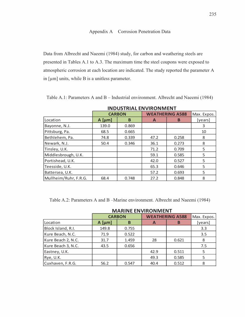
235
Appendix A Corrosion Penetration Data
Data from Albrecht and Naeemi (1984) study, for carbon and weathering steels are
presented in Tables A.1 to A.3. The maximum time the steel coupons were exposed to
atmospheric corrosion at each location are indicated. The study reported the parameter A
in [µm] units, while B is a unitless parameter.
Table A.1: Parameters A and B – Industrial environment. Albrecht and Naeemi (1984)
Table A.2: Parameters A and B –Marine environment. Albrecht and Naeemi (1984)
Max. Expos.
Location A [μm] B A B [years]
Bayonne, N.J. 139.0 0.869 3
Pittsburg, Pa. 68.5 0.665 10
Bethlehem, Pa. 74.8 0.339 47.2 0.258 8
Newark, N.J. 50.4 0.346 36.1 0.273 8
Tinsley, U.K. 71.2 0.709 5
Middlesbrough, U.K. 59.1 0.585 5
Portishead, U.K. 42.0 0.527 5
Teesside, U.K. 65.3 0.646 5
Battersea, U.K. 57.2 0.693 5
Mullheim/Ruhr, F.R.G. 68.4 0.748 27.2 0.848 8
INDUSTRIAL ENVIRONMENTCARBON WEATHERING A588
Max. Expos.
Location A [μm] B A B [years]
Block Island, R.I. 149.8 0.755 3.3
Kure Beach, N.C. 71.9 0.522 3.5
Kure Beach 2, N.C. 31.7 1.459 28 0.621 8
Kure Beach 3, N.C. 43.5 0.656 7.5
Eastney, U.K. 42.9 0.511 5
Rye, U.K. 49.3 0.585 5
Cuxhaven, F.R.G. 56.2 0.547 40.4 0.512 8
MARINE ENVIRONMENTCARBON WEATHERING A588
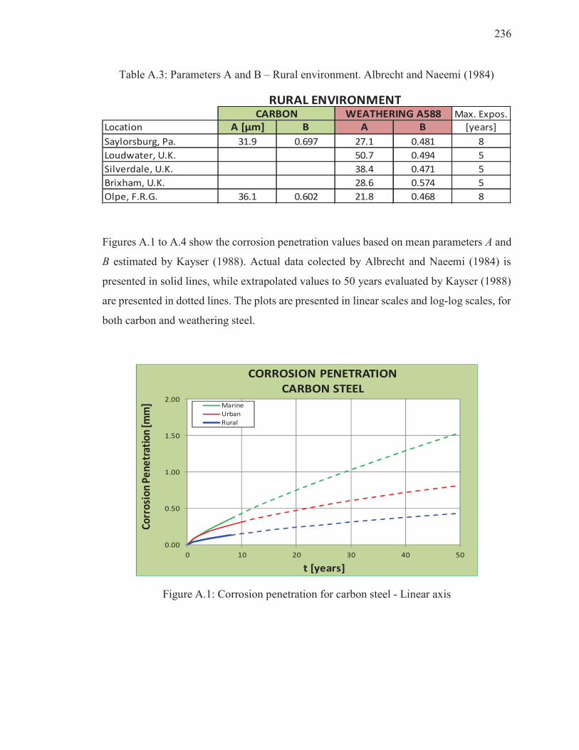
236
Table A.3: Parameters A and B – Rural environment. Albrecht and Naeemi (1984)
Figures A.1 to A.4 show the corrosion penetration values based on mean parameters A and
B estimated by Kayser (1988). Actual data colected by Albrecht and Naeemi (1984) is
presented in solid lines, while extrapolated values to 50 years evaluated by Kayser (1988)
are presented in dotted lines. The plots are presented in linear scales and log-log scales, for
both carbon and weathering steel.
0.00
0.50
1.00
1.50
2.00
0 10 20 30 40 50
Co
rro
sio
n P
en
etr
atio
n [m
m]
t [years]
CORROSION PENETRATION
CARBON STEEL
Marine
Urban
Rural
Figure A.1: Corrosion penetration for carbon steel - Linear axis
Max. Expos.
Location A [μm] B A B [years]
Saylorsburg, Pa. 31.9 0.697 27.1 0.481 8
Loudwater, U.K. 50.7 0.494 5
Silverdale, U.K. 38.4 0.471 5
Brixham, U.K. 28.6 0.574 5
Olpe, F.R.G. 36.1 0.602 21.8 0.468 8
RURAL ENVIRONMENTCARBON WEATHERING A588
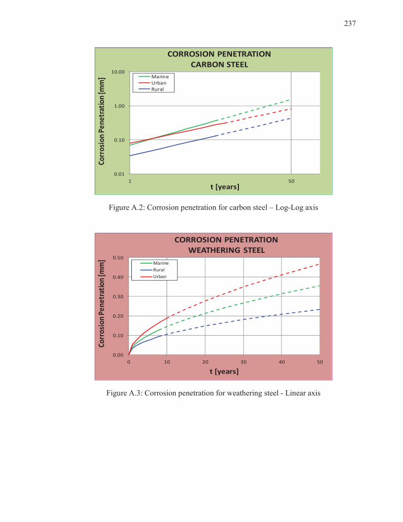
237
0.01
0.10
1.00
10.00
1 50
Co
rro
sio
n P
en
etr
atio
n [m
m]
t [years]
CORROSION PENETRATION
CARBON STEEL
Marine
Urban
Rural
Figure A.2: Corrosion penetration for carbon steel – Log-Log axis
0.00
0.10
0.20
0.30
0.40
0.50
0 10 20 30 40 50
Co
rro
sio
n P
en
etr
atio
n [m
m]
t [years]
CORROSION PENETRATION
WEATHERING STEEL
Marine
Rural
Urban
Figure A.3: Corrosion penetration for weathering steel - Linear axis
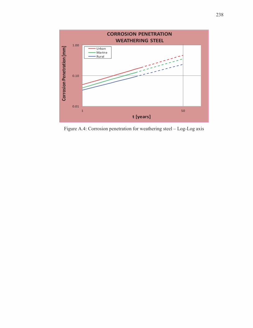
238
0.01
0.10
1.00
1 50
Co
rro
sio
n P
en
etr
atio
n [m
m]
t [years]
CORROSION PENETRATION
WEATHERING STEEL
Urban
Marine
Rural
Figure A.4: Corrosion penetration for weathering steel – Log-Log axis
239
Appendix B Product Certificate
1. Material Test Report for Carbon Steel GR50 from EVRAZ, INC.
2. Report of Test and Analyses for Weathering Steel GR50W from
ARCELORMITTAL STEEL USA
3. Certificate of Analysis for Sodium Chloride from MORTON SALT, INC.
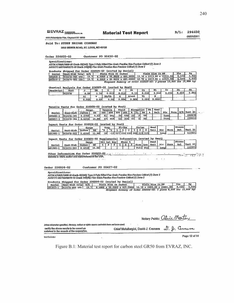
240
Figure B.1: Material test report for carbon steel GR50 from EVRAZ, INC.
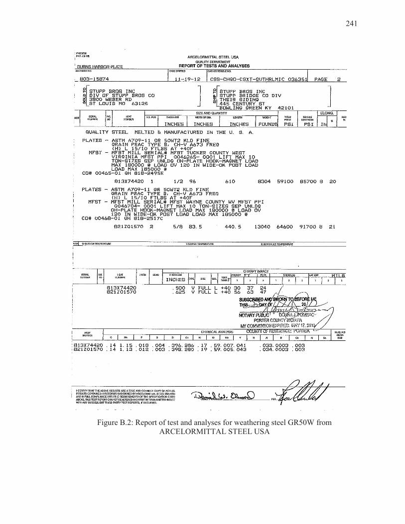
241
Figure B.2: Report of test and analyses for weathering steel GR50W from ARCELORMITTAL STEEL USA
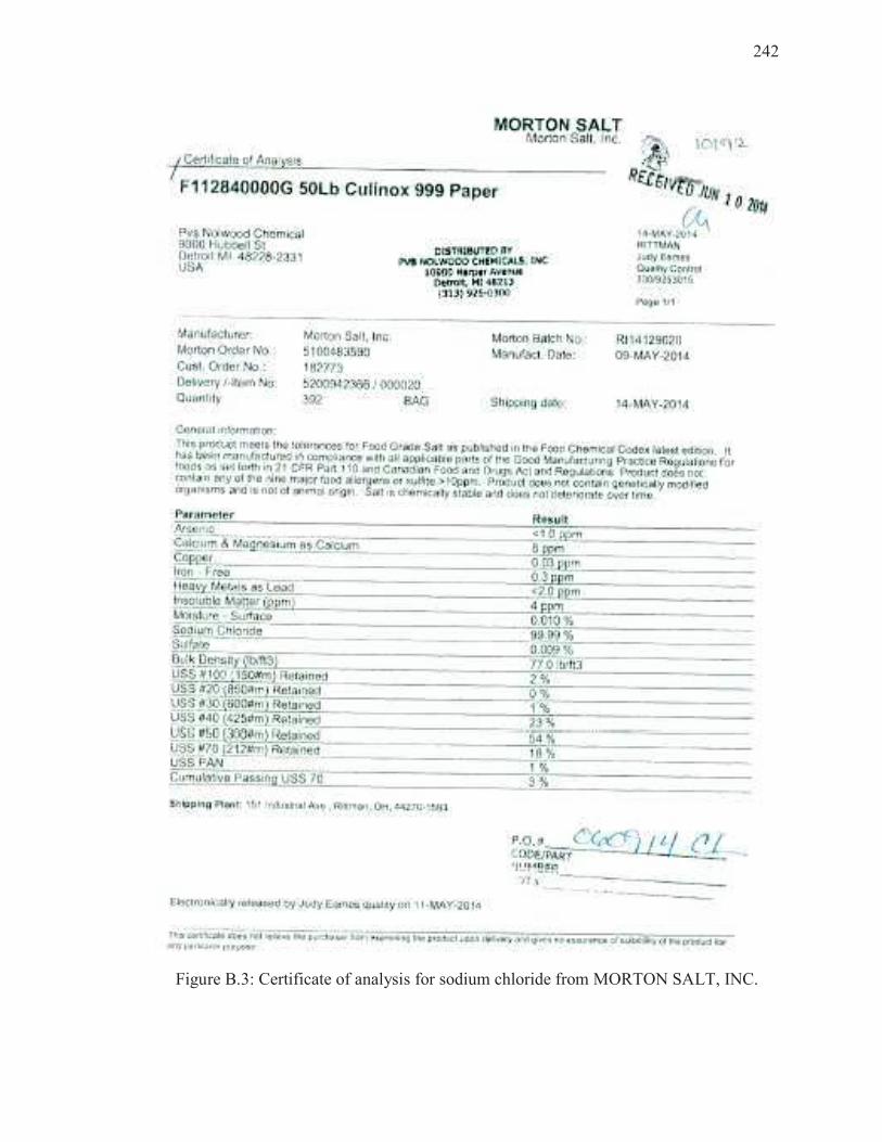
242
Figure B.3: Certificate of analysis for sodium chloride from MORTON SALT, INC.

243
Appendix C Identification of Coupons for ACT
The coupon identification system is presented herein. Steel Type A involves uncoated
carbon steel, and it is comprised by Groups A01 to A10. Steel Type B involves coated
carbon steel, and it is comprised by Groups B01 to B10. Steel Type C involves uncoated
weathering steel, and it is comprised by Groups C01 to C10. Steel Type D involves
coated carbon steel with a scratch mark, and it is comprised by Groups D01 to D07.
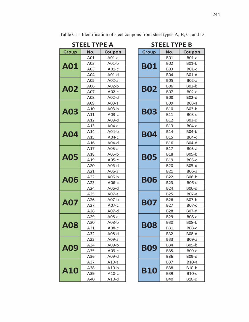
244
Table C.1: Identification of steel coupons from steel types A, B, C, and D
Group No. Coupon Group No. Coupon
A01 A01-a B01 B01-a
A02 A01-b B02 B01-b
A03 A01-c B03 B01-c
A04 A01-d B04 B01-d
A05 A02-a B05 B02-a
A06 A02-b B06 B02-b
A07 A02-c B07 B02-c
A08 A02-d B08 B02-d
A09 A03-a B09 B03-a
A10 A03-b B10 B03-b
A11 A03-c B11 B03-c
A12 A03-d B12 B03-d
A13 A04-a B13 B04-a
A14 A04-b B14 B04-b
A15 A04-c B15 B04-c
A16 A04-d B16 B04-d
A17 A05-a B17 B05-a
A18 A05-b B18 B05-b
A19 A05-c B19 B05-c
A20 A05-d B20 B05-d
A21 A06-a B21 B06-a
A22 A06-b B22 B06-b
A23 A06-c B23 B06-c
A24 A06-d B24 B06-d
A25 A07-a B25 B07-a
A26 A07-b B26 B07-b
A27 A07-c B27 B07-c
A28 A07-d B28 B07-d
A29 A08-a B29 B08-a
A30 A08-b B30 B08-b
A31 A08-c B31 B08-c
A32 A08-d B32 B08-d
A33 A09-a B33 B09-a
A34 A09-b B34 B09-b
A35 A09-c B35 B09-c
A36 A09-d B36 B09-d
A37 A10-a B37 B10-a
A38 A10-b B38 B10-b
A39 A10-c B39 B10-c
A40 A10-d B40 B10-d
B08
B09
B10
A08
A09
A10
B01
B02
B03
B04
B05
B06
A01
A02
A03
A04
A05
A06
B07
STEEL TYPE A STEEL TYPE B
A07
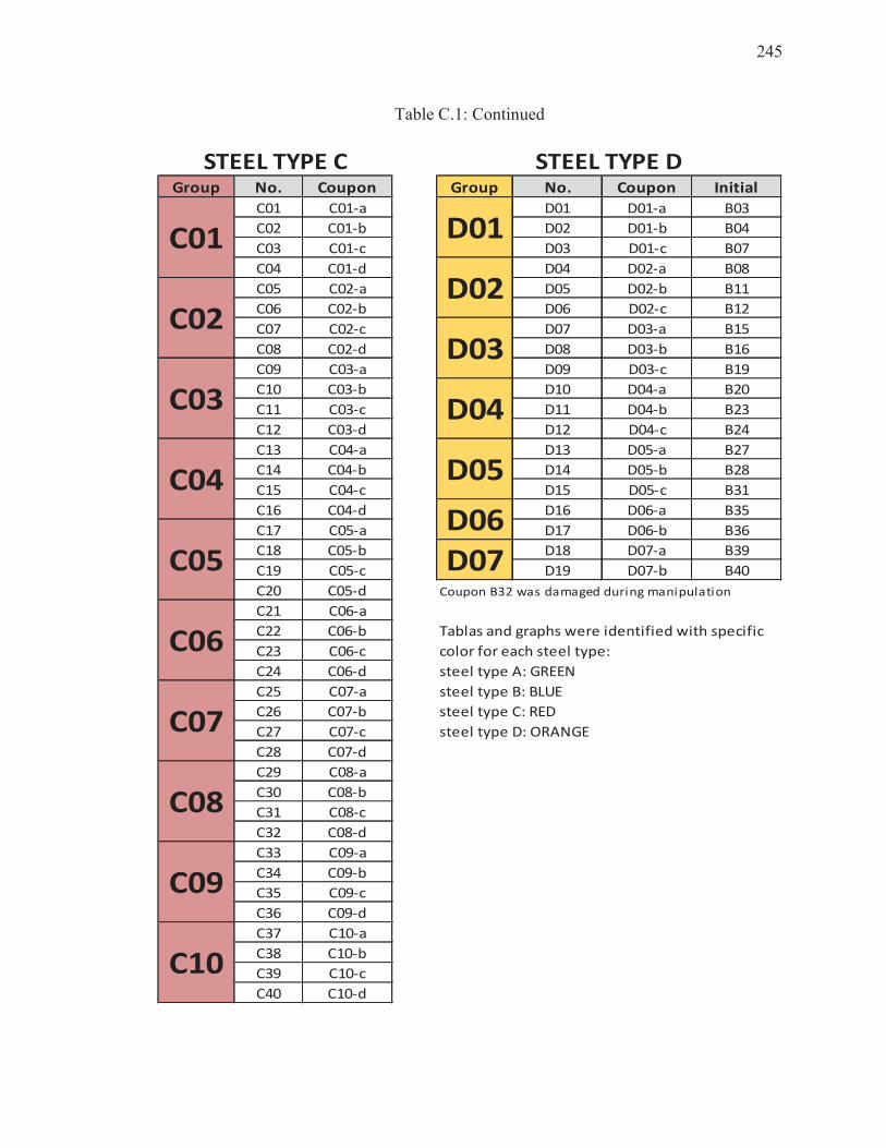
245
Table C.1: Continued
Group No. Coupon Group No. Coupon Initial
C01 C01-a D01 D01-a B03
C02 C01-b D02 D01-b B04
C03 C01-c D03 D01-c B07
C04 C01-d D04 D02-a B08
C05 C02-a D05 D02-b B11
C06 C02-b D06 D02-c B12
C07 C02-c D07 D03-a B15
C08 C02-d D08 D03-b B16
C09 C03-a D09 D03-c B19
C10 C03-b D10 D04-a B20
C11 C03-c D11 D04-b B23
C12 C03-d D12 D04-c B24
C13 C04-a D13 D05-a B27
C14 C04-b D14 D05-b B28
C15 C04-c D15 D05-c B31
C16 C04-d D16 D06-a B35
C17 C05-a D17 D06-b B36
C18 C05-b D18 D07-a B39
C19 C05-c D19 D07-b B40
C20 C05-d Coupon B32 was damaged during manipulation
C21 C06-a
C22 C06-b Tablas and graphs were identified with specific
C23 C06-c color for each steel type:
C24 C06-d steel type A: GREEN
C25 C07-a steel type B: BLUE
C26 C07-b steel type C: RED
C27 C07-c steel type D: ORANGE
C28 C07-d
C29 C08-a
C30 C08-b
C31 C08-c
C32 C08-d
C33 C09-a
C34 C09-b
C35 C09-c
C36 C09-d
C37 C10-a
C38 C10-b
C39 C10-c
C40 C10-d
C06
D01
D02
D03
D04
D05
D07
C07
C08
C09
C10
D06
C01
C02
C03
C04
C05
STEEL TYPE DSTEEL TYPE C

246
Appendix D Weight Change During ACT
The weight change for each steel coupon is presented in this Appendix, in tabulated and
graphical manner. Weight changes for coupons from steel Types A, B, and C are
presented week by week for the 24 weeks the ACT lasted. For coupons from steel Type
D the data are presented for the 10 weeks they were under the ACT. The data are
presented for each steel type and for each group, every week a group was subjected to
washing.
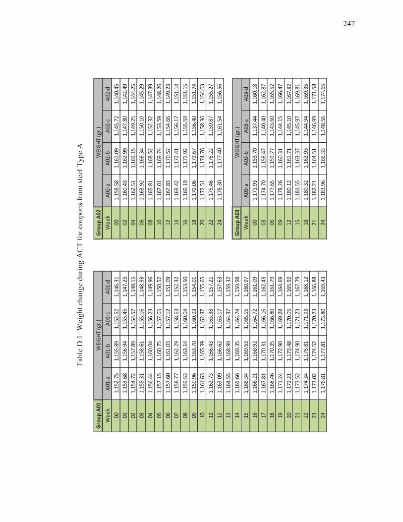
247
Tab
le D
.1:
Wei
gh
t ch
ang
e d
uri
ng A
CT
fo
r co
up
on
s fr
om
ste
el T
yp
e A
Gro
up
A01
Gro
up
A02
We
ek
A01
-aA
01-b
A01
-cA
01-d
We
ek
A02
-aA
02-b
A02
-cA
02-d
001,
152.
751,
155.
891,
152.
521,
146.
3100
1,15
8.58
1,16
1.09
1,14
5.72
1,14
0.45
011,
153.
681,
156.
941,
153.
451,
147.
2502
1,16
0.43
1,16
2.99
1,14
7.80
1,14
2.49
021,
154.
721,
157.
891,
154.
571,
148.
1504
1,16
2.51
1,16
5.15
1,14
9.25
1,14
4.25
031,
155.
311,
158.
611,
155.
161,
148.
9306
1,16
3.92
1,16
6.34
1,15
0.10
1,14
5.29
041,
156.
441,
160.
041,
156.
231,
149.
9608
1,16
5.81
1,16
8.52
1,15
2.32
1,14
7.39
051,
157.
151,
160.
751,
157.
051,
150.
5210
1,16
7.01
1,16
9.74
1,15
3.59
1,14
8.26
061,
157.
601,
161.
031,
157.
121,
151.
0912
1,16
7.83
1,17
0.52
1,15
4.66
1,14
9.23
071,
158.
771,
162.
291,
158.
631,
152.
3214
1,16
9.42
1,17
2.41
1,15
6.17
1,15
1.14
081,
159.
531,
163.
141,
160.
041,
153.
5016
1,16
9.19
1,17
1.92
1,15
5.59
1,15
1.15
091,
159.
961,
163.
701,
160.
931,
154.
0118
1,17
0.06
1,17
2.67
1,15
6.40
1,15
1.74
101,
161.
631,
165.
391,
162.
371,
155.
6520
1,17
2.51
1,17
4.76
1,15
8.36
1,15
4.03
111,
162.
731,
166.
431,
163.
381,
157.
2122
1,17
5.46
1,17
6.22
1,15
9.87
1,15
5.27
121,
163.
091,
166.
621,
163.
171,
157.
6324
1,17
8.30
1,17
7.40
1,16
1.54
1,15
6.56
131,
164.
551,
168.
991,
164.
371,
159.
32
141,
165.
661,
169.
351,
164.
741,
159.
98G
rou
p A
03
151,
166.
341,
169.
531,
165.
151,
160.
97W
ee
kA
03-a
A03
-bA
03-c
A03
-d
161,
166.
211,
168.
921,
164.
721,
161.
0900
1,17
1.93
1,15
3.70
1,13
7.44
1,16
0.18
171,
167.
811,
170.
311,
166.
161,
162.
4303
1,17
4.70
1,15
6.47
1,14
0.40
1,16
2.87
181,
168.
461,
170.
351,
166.
801,
161.
7906
1,17
7.65
1,15
9.77
1,14
3.60
1,16
5.52
191,
171.
241,
172.
901,
169.
281,
164.
6909
1,17
8.26
1,16
0.31
1,14
4.15
1,16
6.47
201,
172.
211,
173.
481,
170.
051,
165.
9212
1,18
0.12
1,16
1.71
1,14
5.10
1,16
7.82
211,
173.
521,
174.
901,
171.
231,
167.
7915
1,18
1.55
1,16
3.37
1,14
5.97
1,16
9.81
221,
174.
341,
175.
811,
171.
931,
168.
1218
1,18
0.32
1,16
2.93
1,14
4.94
1,16
9.35
231,
173.
021,
174.
521,
170.
731,
166.
8821
1,18
2.21
1,16
4.51
1,14
6.99
1,17
1.58
241,
176.
811,
177.
811,
173.
801,
169.
4324
1,18
3.96
1,16
6.33
1,14
8.56
1,17
4.65
WEI
GH
T (g
r.)
WEI
GH
T (g
r.)
WEI
GH
T (g
r.)
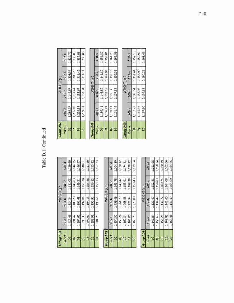
248
Tab
le D
.1:
Co
nti
nu
ed
Gro
up
A0
4G
rou
p A
07
We
ek
A0
4-a
A0
4-b
A0
4-c
A0
4-d
We
ek
A0
7-a
A0
7-b
A0
7-c
A0
7-d
00
1,2
87
.46
1,1
84
.34
1,1
41
.08
1,1
39
.69
00
1,2
89
.97
1,1
44
.67
1,3
03
.57
1,3
29
.77
04
1,2
91
.47
1,1
88
.28
1,1
45
.83
1,1
44
.25
07
1,2
96
.10
1,1
51
.44
1,3
09
.78
1,3
36
.08
08
1,2
94
.62
1,1
91
.63
1,1
49
.31
1,1
46
.97
14
1,2
98
.55
1,1
53
.62
1,3
11
.49
1,3
39
.06
12
1,2
95
.33
1,1
92
.84
1,1
51
.38
1,1
48
.81
21
1,2
99
.01
1,1
53
.31
1,3
11
.11
1,3
39
.86
16
1,2
96
.97
1,1
94
.13
1,1
53
.46
1,1
51
.19
20
1,2
98
.91
1,1
95
.91
1,1
56
.12
1,1
53
.32
Gro
up
A0
8
24
1,3
01
.25
1,1
98
.61
1,1
59
.73
1,1
57
.33
We
ek
A0
8-a
A0
8-b
A0
8-c
A0
8-d
00
1,1
50
.41
1,1
46
.89
1,1
41
.80
1,1
51
.87
Gro
up
A0
50
81
,15
6.7
11
,15
3.1
81
,14
7.9
31
,15
8.0
1
We
ek
A0
5-a
A0
5-b
A0
5-c
A0
5-d
16
1,1
59
.11
1,1
55
.30
1,1
52
.13
1,1
61
.25
00
1,1
54
.30
1,2
59
.49
1,1
43
.78
1,1
64
.80
24
1,1
61
.45
1,1
57
.89
1,1
55
.33
1,1
63
.39
05
1,1
59
.24
1,2
64
.79
1,1
49
.42
1,1
70
.12
10
1,1
62
.84
1,2
68
.58
1,1
53
.91
1,1
74
.41
Gro
up
A0
9
15
1,1
65
.00
1,2
71
.94
1,1
58
.28
1,1
78
.22
We
ek
A0
9-a
A0
9-b
A0
9-c
A0
9-d
20
1,1
65
.75
1,2
73
.08
1,1
59
.43
1,1
79
.54
00
1,1
57
.73
1,1
45
.54
1,1
51
.41
1,1
52
.15
09
1,1
65
.32
1,1
52
.98
1,1
58
.90
1,1
59
.91
Gro
up
A0
61
81
,16
7.6
01
,15
4.3
21
,16
0.2
91
,16
3.4
6
We
ek
A0
6-a
A0
6-b
A0
6-c
A0
6-d
00
1,1
49
.84
1,1
27
.47
1,1
52
.23
1,1
51
.98
06
1,1
56
.63
1,1
34
.42
1,1
58
.83
1,1
58
.74
12
1,1
58
.26
1,1
36
.72
1,1
60
.74
1,1
60
.19
18
1,1
62
.83
1,1
41
.40
1,1
64
.08
1,1
62
.56
24
1,1
63
.41
1,1
41
.39
1,1
64
.69
1,1
64
.65
WE
IGH
T (
gr.
)
WE
IGH
T (
gr.
)
WE
IGH
T (
gr.
)
WE
IGH
T (
gr.
)
WE
IGH
T (
gr.
)
WE
IGH
T (
gr.
)
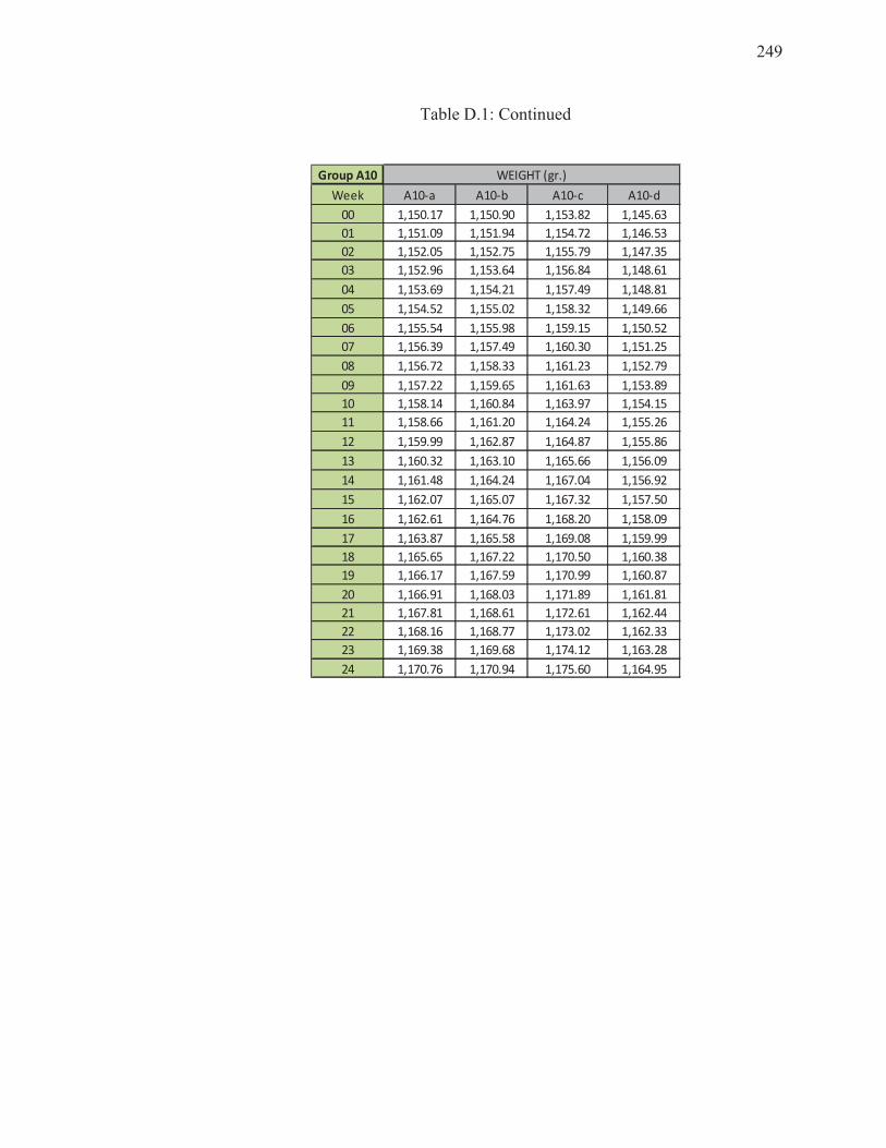
249
Table D.1: Continued
Group A10
Week A10-a A10-b A10-c A10-d
00 1,150.17 1,150.90 1,153.82 1,145.63
01 1,151.09 1,151.94 1,154.72 1,146.53
02 1,152.05 1,152.75 1,155.79 1,147.35
03 1,152.96 1,153.64 1,156.84 1,148.61
04 1,153.69 1,154.21 1,157.49 1,148.81
05 1,154.52 1,155.02 1,158.32 1,149.66
06 1,155.54 1,155.98 1,159.15 1,150.52
07 1,156.39 1,157.49 1,160.30 1,151.25
08 1,156.72 1,158.33 1,161.23 1,152.79
09 1,157.22 1,159.65 1,161.63 1,153.89
10 1,158.14 1,160.84 1,163.97 1,154.15
11 1,158.66 1,161.20 1,164.24 1,155.26
12 1,159.99 1,162.87 1,164.87 1,155.86
13 1,160.32 1,163.10 1,165.66 1,156.09
14 1,161.48 1,164.24 1,167.04 1,156.92
15 1,162.07 1,165.07 1,167.32 1,157.50
16 1,162.61 1,164.76 1,168.20 1,158.09
17 1,163.87 1,165.58 1,169.08 1,159.99
18 1,165.65 1,167.22 1,170.50 1,160.38
19 1,166.17 1,167.59 1,170.99 1,160.87
20 1,166.91 1,168.03 1,171.89 1,161.81
21 1,167.81 1,168.61 1,172.61 1,162.44
22 1,168.16 1,168.77 1,173.02 1,162.33
23 1,169.38 1,169.68 1,174.12 1,163.28
24 1,170.76 1,170.94 1,175.60 1,164.95
WEIGHT (gr.)
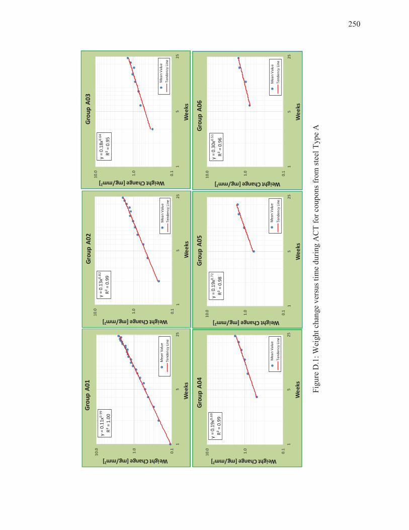
250
Fig
ure
D.1
: W
eigh
t ch
ange
ver
sus
tim
e d
uri
ng A
CT
fo
r co
up
on
s fr
om
ste
el T
yp
e A
y =
0.1
1x0
.99
R²
= 1
.00
0.1
1.0
10
.0
15
25
Weight Change [mg/mm2]
We
ek
s
Gro
up
A0
1
Me
an
Va
lue
Te
nd
en
cy L
ine
y =
0.1
3x0
.82
R²
= 0
.99
0.1
1.0
10
.0
15
25
Weight Change [mg/mm2]
We
ek
s
Gro
up
A0
2
Me
an
Va
lue
Te
nd
en
cy L
ine
y =
0.1
8x0
.64
R²
= 0
.95
0.1
1.0
10
.0
15
25
Weight Change [mg/mm2]
We
ek
s
Gro
up
A0
3
Me
an
Va
lue
Te
nd
en
cy L
ine
y =
0.1
9x0
.69
R²
= 0
.99
0.1
1.0
10
.0
15
25
Weight Change [mg/mm2]
We
ek
s
Gro
up
A0
4
Me
an
Va
lue
Te
nd
en
cy L
ine
y =
0.1
9x0
.72
R²
= 0
.98
0.1
1.0
10
.0
15
25
Weight Change [mg/mm2]
We
ek
s
Gro
up
A0
5
Me
an
Va
lue
Te
nd
en
cy L
ine
y =
0.3
0x0
.51
R²
= 0
.96
0.1
1.0
10
.0
15
25
Weight Change [mg/mm2]
We
ek
s
Gro
up
A0
6
Me
an
Va
lue
Te
nd
en
cy L
ine
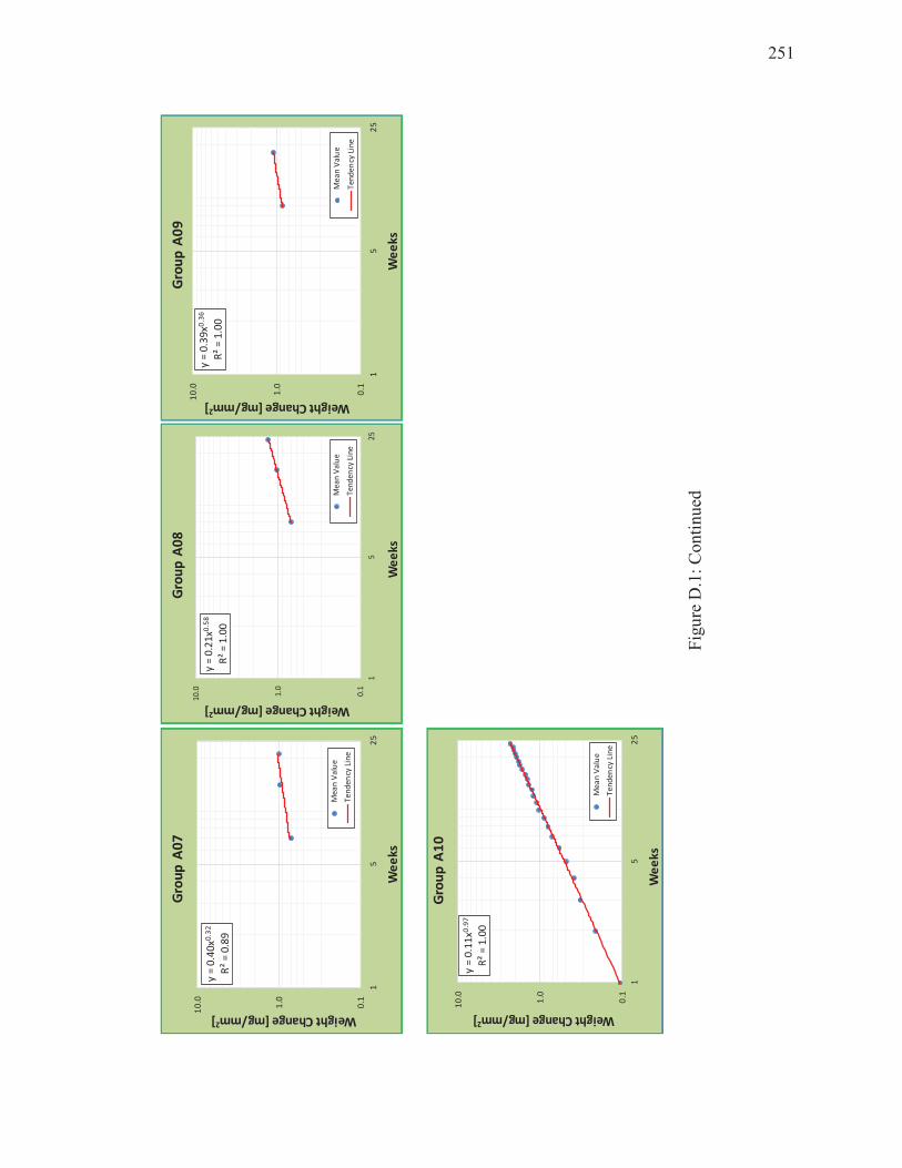
251
Fig
ure
D.1
: C
on
tin
ued
y =
0.4
0x0
.32
R²
= 0
.89
0.1
1.0
10
.0
15
25
Weight Change [mg/mm2]
We
ek
s
Gro
up
A0
7
Me
an
Va
lue
Te
nd
en
cy L
ine
y =
0.2
1x0
.58
R²
= 1
.00
0.1
1.0
10
.0
15
25
Weight Change [mg/mm2]
We
ek
s
Gro
up
A0
8
Me
an
Va
lue
Te
nd
en
cy L
ine
y =
0.3
9x0
.36
R²
= 1
.00
0.1
1.0
10
.0
15
25
Weight Change [mg/mm2]
We
ek
s
Gro
up
A0
9
Me
an
Va
lue
Te
nd
en
cy L
ine
y =
0.1
1x0
.97
R²
= 1
.00
0.1
1.0
10
.0
15
25
Weight Change [mg/mm2]
We
ek
s
Gro
up
A1
0
Me
an
Va
lue
Te
nd
en
cy L
ine
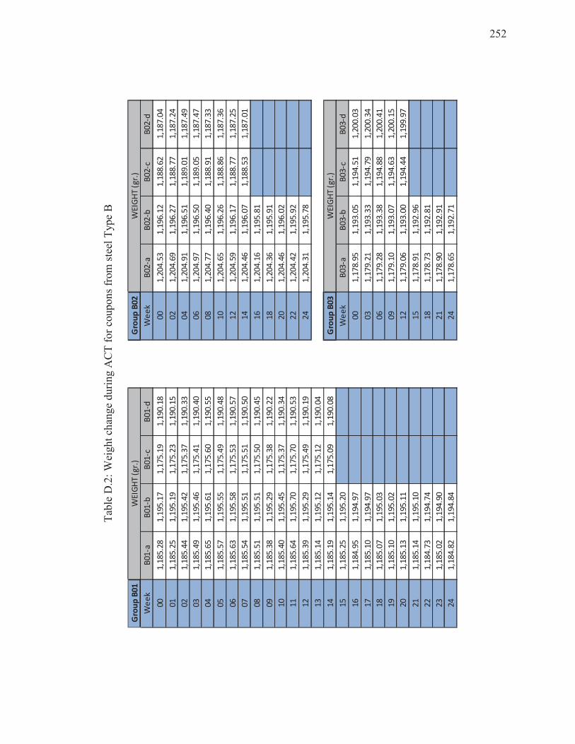
252
Tab
le D
.2:
Wei
gh
t ch
ang
e d
uri
ng A
CT
fo
r co
up
on
s fr
om
ste
el T
yp
e B
Gro
up
B0
1G
rou
p B
02
We
ek
B0
1-a
B0
1-b
B0
1-c
B0
1-d
We
ek
B0
2-a
B0
2-b
B0
2-c
B0
2-d
00
1,1
85
.28
1,1
95
.17
1,1
75
.19
1,1
90
.18
00
1,2
04
.53
1,1
96
.12
1,1
88
.62
1,1
87
.04
01
1,1
85
.25
1,1
95
.19
1,1
75
.23
1,1
90
.15
02
1,2
04
.69
1,1
96
.27
1,1
88
.77
1,1
87
.24
02
1,1
85
.44
1,1
95
.42
1,1
75
.37
1,1
90
.33
04
1,2
04
.91
1,1
96
.51
1,1
89
.01
1,1
87
.49
03
1,1
85
.49
1,1
95
.46
1,1
75
.41
1,1
90
.40
06
1,2
04
.97
1,1
96
.50
1,1
89
.05
1,1
87
.47
04
1,1
85
.65
1,1
95
.61
1,1
75
.60
1,1
90
.55
08
1,2
04
.77
1,1
96
.40
1,1
88
.91
1,1
87
.33
05
1,1
85
.57
1,1
95
.55
1,1
75
.49
1,1
90
.48
10
1,2
04
.65
1,1
96
.26
1,1
88
.86
1,1
87
.36
06
1,1
85
.63
1,1
95
.58
1,1
75
.53
1,1
90
.57
12
1,2
04
.59
1,1
96
.17
1,1
88
.77
1,1
87
.25
07
1,1
85
.54
1,1
95
.51
1,1
75
.51
1,1
90
.50
14
1,2
04
.46
1,1
96
.07
1,1
88
.53
1,1
87
.01
08
1,1
85
.51
1,1
95
.51
1,1
75
.50
1,1
90
.45
16
1,2
04
.16
1,1
95
.81
09
1,1
85
.38
1,1
95
.29
1,1
75
.38
1,1
90
.22
18
1,2
04
.36
1,1
95
.91
10
1,1
85
.40
1,1
95
.45
1,1
75
.37
1,1
90
.34
20
1,2
04
.46
1,1
96
.02
11
1,1
85
.64
1,1
95
.70
1,1
75
.70
1,1
90
.53
22
1,2
04
.42
1,1
95
.92
12
1,1
85
.39
1,1
95
.29
1,1
75
.49
1,1
90
.19
24
1,2
04
.31
1,1
95
.78
13
1,1
85
.14
1,1
95
.12
1,1
75
.12
1,1
90
.04
14
1,1
85
.19
1,1
95
.14
1,1
75
.09
1,1
90
.08
Gro
up
B0
3
15
1,1
85
.25
1,1
95
.20
We
ek
B0
3-a
B0
3-b
B0
3-c
B0
3-d
16
1,1
84
.95
1,1
94
.97
00
1,1
78
.95
1,1
93
.05
1,1
94
.51
1,2
00
.03
17
1,1
85
.10
1,1
94
.97
03
1,1
79
.21
1,1
93
.33
1,1
94
.79
1,2
00
.34
18
1,1
85
.07
1,1
95
.03
06
1,1
79
.28
1,1
93
.38
1,1
94
.88
1,2
00
.41
19
1,1
85
.10
1,1
95
.02
09
1,1
79
.10
1,1
93
.07
1,1
94
.63
1,2
00
.15
20
1,1
85
.13
1,1
95
.11
12
1,1
79
.06
1,1
93
.00
1,1
94
.44
1,1
99
.97
21
1,1
85
.14
1,1
95
.10
15
1,1
78
.91
1,1
92
.96
22
1,1
84
.73
1,1
94
.74
18
1,1
78
.73
1,1
92
.81
23
1,1
85
.02
1,1
94
.90
21
1,1
78
.90
1,1
92
.91
24
1,1
84
.82
1,1
94
.84
24
1,1
78
.65
1,1
92
.71
WE
IGH
T (
gr.
)
WE
IGH
T (
gr.
)
WE
IGH
T (
gr.
)
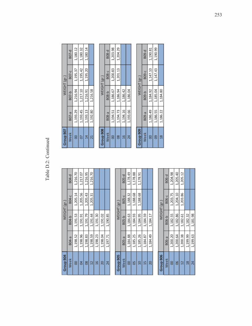
253
Tab
le D
.2:
Co
nti
nu
ed
Gro
up
B0
4G
rou
p B
07
We
ek
B0
4-a
B0
4-b
B0
4-c
B0
4-d
We
ek
B0
7-a
B0
7-b
B0
7-c
B0
7-d
00
1,1
98
.52
1,1
91
.53
1,2
05
.14
1,2
16.
70
00
1,1
93
.29
1,2
16
.94
1,1
95
.37
1,1
80
.12
04
1,1
98
.96
1,1
91
.91
1,2
05
.56
1,2
17.
07
07
1,1
93
.45
1,2
17
.10
1,1
95
.42
1,1
80
.32
08
1,1
98
.83
1,1
91
.79
1,2
05
.43
1,2
16.
95
14
1,1
93
.13
1,2
16
.91
1,1
95
.20
1,1
80
.14
12
1,1
98
.59
1,1
91
.44
1,2
05
.31
1,2
16.
70
21
1,1
92
.80
1,2
16
.58
16
1,1
98
.23
1,1
91
.30
20
1,1
98
.04
1,1
91
.02
Gro
up
B08
24
1,1
97
.71
1,1
90
.85
We
ek
B0
8-a
B0
8-b
B0
8-c
B0
8-d
00
1,1
94
.51
1,1
86
.67
1,2
00
.83
1,2
03
.98
Gro
up
B0
50
81
,19
4.7
31
,18
6.9
41
,20
1.1
31
,20
4.2
9
We
ek
B0
5-a
B0
5-b
B0
5-c
B0
5-d
16
1,1
94.1
61
,18
6.4
2
00
1,1
84
.88
1,1
84
.63
1,1
88
.32
1,1
78.
49
24
1,1
93
.66
1,1
86
.04
05
1,1
85
.25
1,1
84
.93
1,1
88
.68
1,1
78.
88
10
1,1
85
.26
1,1
84
.95
1,1
88
.68
1,1
78.
91
Gro
up
B09
15
1,1
84
.87
1,1
84
.59
We
ek
B0
9-a
B0
9-b
B0
9-c
B0
9-d
20
1,1
84
.49
1,1
84
.17
00
1,1
86
.49
1,1
84
.92
1,1
47
.10
1,1
90
.81
09
1,1
86
.55
1,1
85
.04
1,1
47
.43
1,1
90
.99
Gro
up
B0
61
81
,18
6.2
21
,18
4.8
0
We
ek
B0
6-a
B0
6-b
B0
6-c
B0
6-d
00
1,2
00
.20
1,1
82
.55
1,2
03
.75
1,2
04.
98
06
1,2
00
.64
1,1
82
.86
1,2
04
.10
1,2
05.
40
12
1,2
00
.38
1,1
82
.61
1,2
03
.86
1,2
05.
12
18
1,1
99
.99
1,1
82
.32
24
1,1
99
.63
1,1
81
.98
WE
IGH
T (
gr.
)
WE
IGH
T (
gr.
)
WE
IGH
T (
gr.
)
WE
IGH
T (
gr.
)
WE
IGH
T (
gr.
)
WE
IGH
T (
gr.
)
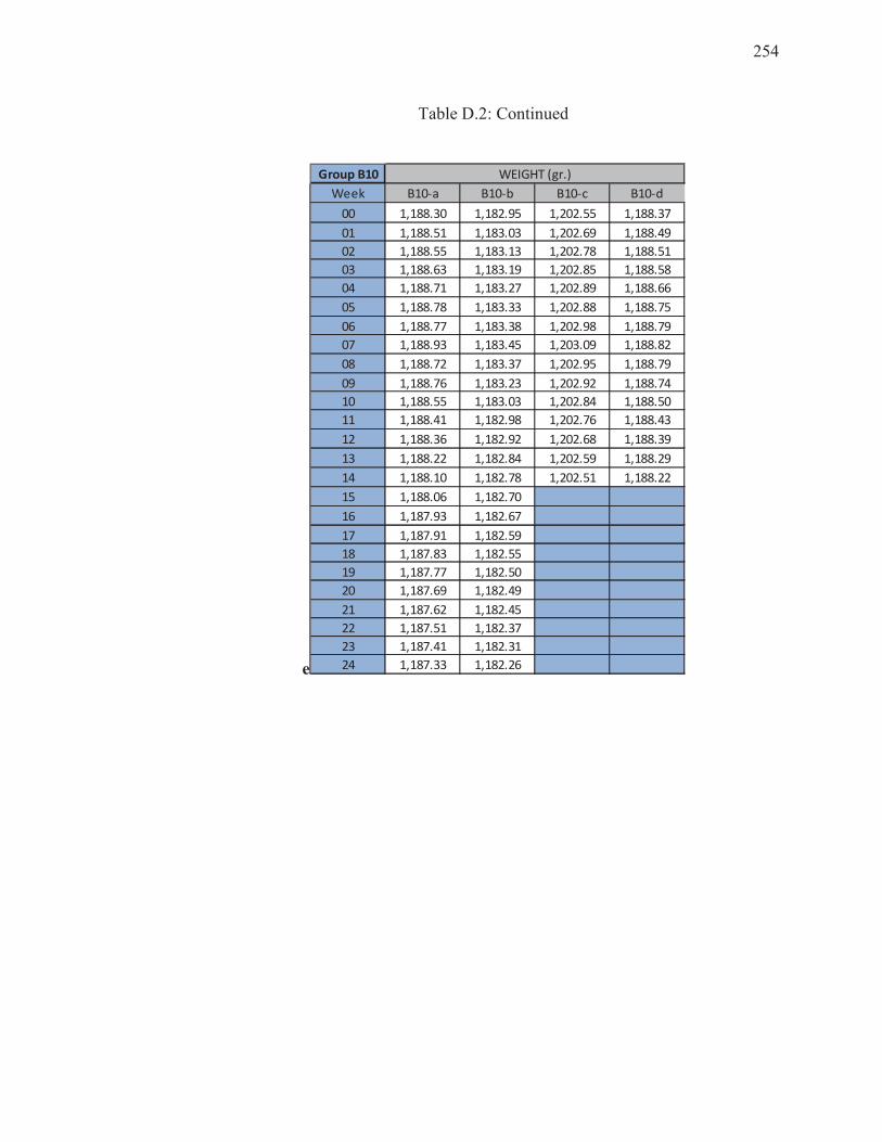
254
Table D.2: Continued
e
Group B10
Week B10-a B10-b B10-c B10-d
00 1,188.30 1,182.95 1,202.55 1,188.37
01 1,188.51 1,183.03 1,202.69 1,188.49
02 1,188.55 1,183.13 1,202.78 1,188.51
03 1,188.63 1,183.19 1,202.85 1,188.58
04 1,188.71 1,183.27 1,202.89 1,188.66
05 1,188.78 1,183.33 1,202.88 1,188.75
06 1,188.77 1,183.38 1,202.98 1,188.79
07 1,188.93 1,183.45 1,203.09 1,188.82
08 1,188.72 1,183.37 1,202.95 1,188.79
09 1,188.76 1,183.23 1,202.92 1,188.74
10 1,188.55 1,183.03 1,202.84 1,188.50
11 1,188.41 1,182.98 1,202.76 1,188.43
12 1,188.36 1,182.92 1,202.68 1,188.39
13 1,188.22 1,182.84 1,202.59 1,188.29
14 1,188.10 1,182.78 1,202.51 1,188.22
15 1,188.06 1,182.70
16 1,187.93 1,182.67
17 1,187.91 1,182.59
18 1,187.83 1,182.55
19 1,187.77 1,182.50
20 1,187.69 1,182.49
21 1,187.62 1,182.45
22 1,187.51 1,182.37
23 1,187.41 1,182.31
24 1,187.33 1,182.26
WEIGHT (gr.)
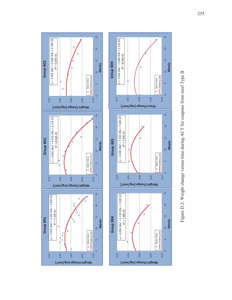
255
Fig
ure
D.2
: W
eigh
t ch
ange
ver
sus
tim
e d
uri
ng A
CT
fo
r co
up
on
s fr
om
ste
el T
yp
e B
y =
-2
.91
E-0
4x2
+ 3
.32
E-0
3x
+ 1
.92
E-0
2
R²
= 7
.34
E-0
1
-0.1
0
-0.0
5
0.0
0
0.0
5
0.1
0
05
10
15
20
25
Weight Change [mg/mm2]
We
ek
s
Gro
up
B0
1
Me
an
Va
lue
Te
nd
en
cy L
ine
y =
-3
.82
E-0
4x2
+ 4
.01
E-0
3x
+ 2
.11
E-0
2
R²
= 8
.94
E-0
1
-0.1
0
-0.0
5
0.0
0
0.0
5
0.1
0
05
10
15
20
25
Weight Change [mg/mm2]
We
ek
s
Gro
up
B0
2
Me
an
Va
lue
Te
nd
en
cy L
ine
y =
-1
.43
E-0
4x2
+ 6
.60
E-0
4x
+ 2
.10
E-0
2
R²
= 6
.85
E-0
1
-0.1
0
-0.0
5
0.0
0
0.0
5
0.1
0
05
10
15
20
25
Weight Change [mg/mm2]
We
ek
s
Gro
up
B0
3
Me
an
Va
lue
Te
nd
en
cy L
ine
y =
-4
.05
E-0
4x2
+ 5
.11
E-0
3x
+ 1
.52
E-0
2
R²
= 7
.48
E-0
1
-0.1
0
-0.0
5
0.0
0
0.0
5
0.1
0
05
10
15
20
25
Weight Change [mg/mm2]
We
eks
Gro
up
B0
4
Me
an
Va
lue
Te
nd
en
cy L
ine
y =
-4
.43
E-0
4x2
+ 7
.45
E-0
3x
+ 7
.64
E-0
3
R²
= 7
.03
E-0
1
-0.1
0
-0.0
5
0.0
0
0.0
5
0.1
0
05
10
15
20
25
Weight Change [mg/mm2]
We
ek
s
Gro
up
B0
5
Me
an
Va
lue
Te
nd
en
cy L
ine
y =
-3
.03
E-0
4x2
+ 3
.46
E-0
3x
+ 1
.12
E-0
2
R²
= 8
.39
E-0
1
-0.1
0
-0.0
5
0.0
0
0.0
5
0.1
0
05
10
15
20
25
Mass Change [mg/mm2]
We
eks
Gro
up
B0
6
Me
an
Va
lue
Te
nd
en
cy L
ine
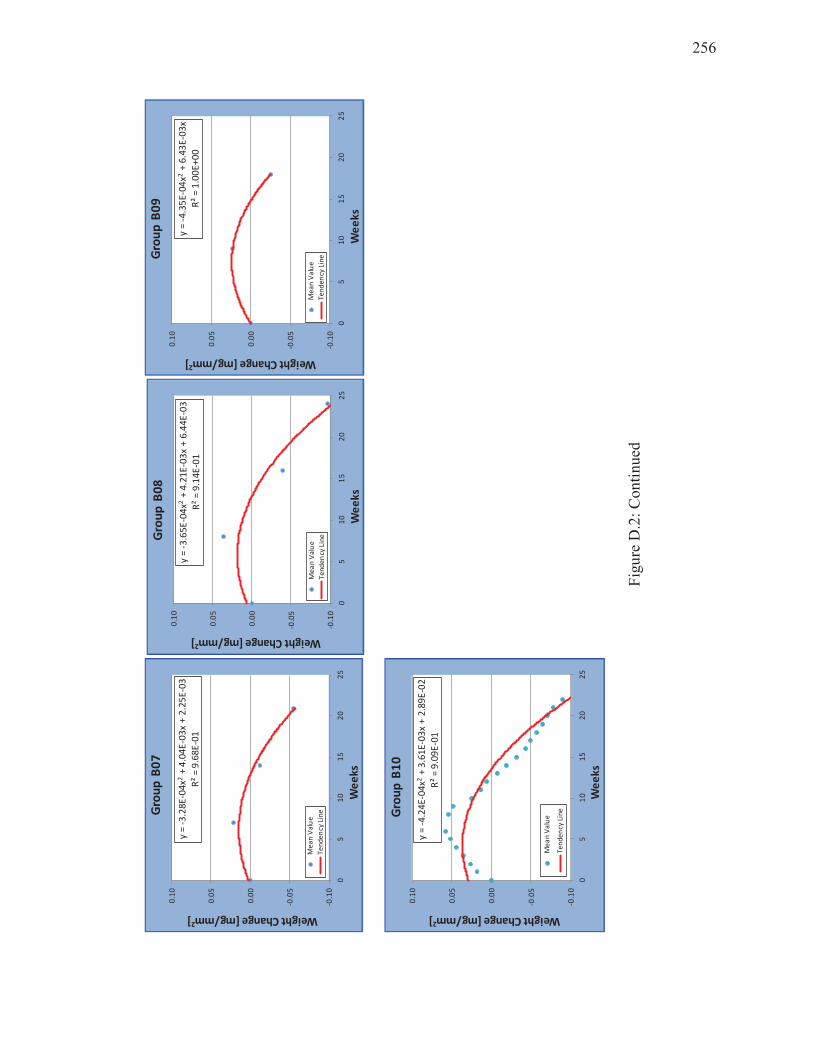
256
Fig
ure
D.2
: C
on
tin
ued
y =
-3
.28
E-0
4x2
+ 4
.04
E-0
3x
+ 2
.25
E-0
3
R²
= 9
.68
E-0
1
-0.1
0
-0.0
5
0.0
0
0.0
5
0.1
0
05
10
15
20
25
Weight Change [mg/mm2]
We
ek
s
Gro
up
B0
7
Me
an
Va
lue
Te
nd
en
cy L
ine
y =
-3
.65
E-0
4x2
+ 4
.21
E-0
3x
+ 6
.44
E-0
3
R²
= 9
.14
E-0
1
-0.1
0
-0.0
5
0.0
0
0.0
5
0.1
0
05
10
15
20
25
Weight Change [mg/mm2]
We
ek
s
Gro
up
B0
8
Me
an
Va
lue
Te
nd
en
cy L
ine
y =
-4
.35
E-0
4x2
+ 6
.43
E-0
3x
R²
= 1
.00
E+
00
-0.1
0
-0.0
5
0.0
0
0.0
5
0.1
0
05
10
15
20
25
Weight Change [mg/mm2]
We
ek
s
Gro
up
B0
9
Me
an
Va
lue
Te
nd
en
cy L
ine
y =
-4
.24
E-0
4x2
+ 3
.61
E-0
3x
+ 2
.89
E-0
2
R²
= 9
.09
E-0
1
-0.1
0
-0.0
5
0.0
0
0.0
5
0.1
0
05
10
15
20
25
Weight Change [mg/mm2]
We
ek
s
Gro
up
B1
0
Me
an
Va
lue
Te
nd
en
cy L
ine
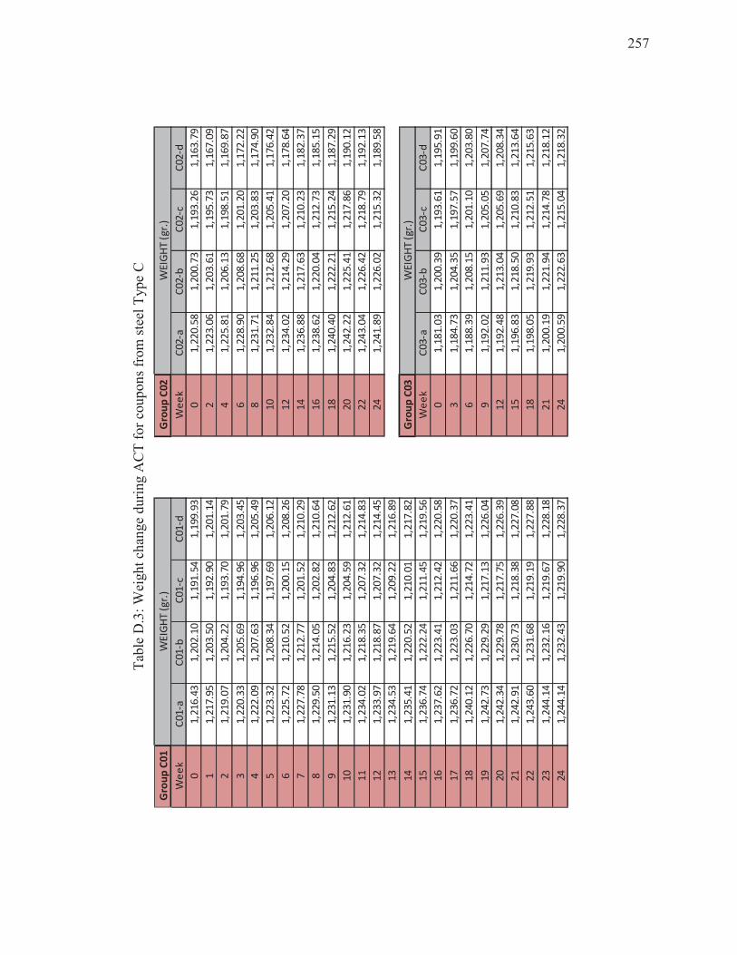
257
Tab
le D
.3:
Wei
gh
t ch
ang
e d
uri
ng A
CT
fo
r co
up
on
s fr
om
ste
el T
yp
e C
Gro
up
C0
1G
rou
p C
02
We
ek
C0
1-a
C0
1-b
C0
1-c
C0
1-d
We
ek
C0
2-a
C0
2-b
C0
2-c
C0
2-d
01
,21
6.4
31
,20
2.1
01
,19
1.5
41
,19
9.9
30
1,2
20
.58
1,2
00
.73
1,1
93
.26
1,1
63
.79
11
,21
7.9
51
,20
3.5
01
,19
2.9
01
,20
1.1
42
1,2
23
.06
1,2
03
.61
1,1
95
.73
1,1
67
.09
21
,21
9.0
71
,20
4.2
21
,19
3.7
01
,20
1.7
94
1,2
25
.81
1,2
06
.13
1,1
98
.51
1,1
69
.87
31
,22
0.3
31
,20
5.6
91
,19
4.9
61
,20
3.4
56
1,2
28
.90
1,2
08
.68
1,2
01
.20
1,1
72
.22
41
,22
2.0
91
,20
7.6
31
,19
6.9
61
,20
5.4
98
1,2
31
.71
1,2
11
.25
1,2
03
.83
1,1
74
.90
51
,22
3.3
21
,20
8.3
41
,19
7.6
91
,20
6.1
21
01
,23
2.8
41
,21
2.6
81
,20
5.4
11
,17
6.4
2
61
,22
5.7
21
,21
0.5
21
,20
0.1
51
,20
8.2
61
21
,23
4.0
21
,21
4.2
91
,20
7.2
01
,17
8.6
4
71
,22
7.7
81
,21
2.7
71
,20
1.5
21
,21
0.2
91
41
,23
6.8
81
,21
7.6
31
,21
0.2
31
,18
2.3
7
81
,22
9.5
01
,21
4.0
51
,20
2.8
21
,21
0.6
41
61
,23
8.6
21
,22
0.0
41
,21
2.7
31
,18
5.1
5
91
,23
1.1
31
,21
5.5
21
,20
4.8
31
,21
2.6
21
81
,24
0.4
01
,22
2.2
11
,21
5.2
41
,18
7.2
9
10
1,2
31
.90
1,2
16
.23
1,2
04
.59
1,2
12
.61
20
1,2
42
.22
1,2
25
.41
1,2
17
.86
1,1
90
.12
11
1,2
34
.02
1,2
18
.35
1,2
07
.32
1,2
14
.83
22
1,2
43
.04
1,2
26
.42
1,2
18
.79
1,1
92
.13
12
1,2
33
.97
1,2
18
.87
1,2
07
.32
1,2
14
.45
24
1,2
41
.89
1,2
26
.02
1,2
15
.32
1,1
89
.58
13
1,2
34
.53
1,2
19
.64
1,2
09
.22
1,2
16
.89
14
1,2
35
.41
1,2
20
.52
1,2
10
.01
1,2
17
.82
Gro
up
C0
3
15
1,2
36
.74
1,2
22
.24
1,2
11
.45
1,2
19
.56
We
ek
C0
3-a
C0
3-b
C0
3-c
C0
3-d
16
1,2
37
.62
1,2
23
.41
1,2
12
.42
1,2
20
.58
01
,18
1.0
31
,20
0.3
91
,19
3.6
11
,19
5.9
1
17
1,2
36
.72
1,2
23
.03
1,2
11
.66
1,2
20
.37
31
,18
4.7
31
,20
4.3
51
,19
7.5
71
,19
9.6
0
18
1,2
40
.12
1,2
26
.70
1,2
14
.72
1,2
23
.41
61
,18
8.3
91
,20
8.1
51
,20
1.1
01
,20
3.8
0
19
1,2
42
.73
1,2
29
.29
1,2
17
.13
1,2
26
.04
91
,19
2.0
21
,21
1.9
31
,20
5.0
51
,20
7.7
4
20
1,2
42
.34
1,2
29
.78
1,2
17
.75
1,2
26
.39
12
1,1
92
.48
1,2
13
.04
1,2
05
.69
1,2
08
.34
21
1,2
42
.91
1,2
30
.73
1,2
18
.38
1,2
27
.08
15
1,1
96
.83
1,2
18
.50
1,2
10
.83
1,2
13
.64
22
1,2
43
.60
1,2
31
.68
1,2
19
.19
1,2
27
.88
18
1,1
98
.05
1,2
19
.93
1,2
12
.51
1,2
15
.63
23
1,2
44
.14
1,2
32
.16
1,2
19
.67
1,2
28
.18
21
1,2
00
.19
1,2
21
.94
1,2
14
.78
1,2
18
.12
24
1,2
44
.14
1,2
32
.43
1,2
19
.90
1,2
28
.37
24
1,2
00
.59
1,2
22
.63
1,2
15
.04
1,2
18
.32
WE
IGH
T (
gr.
)
WE
IGH
T (
gr.
)W
EIG
HT
(g
r.)
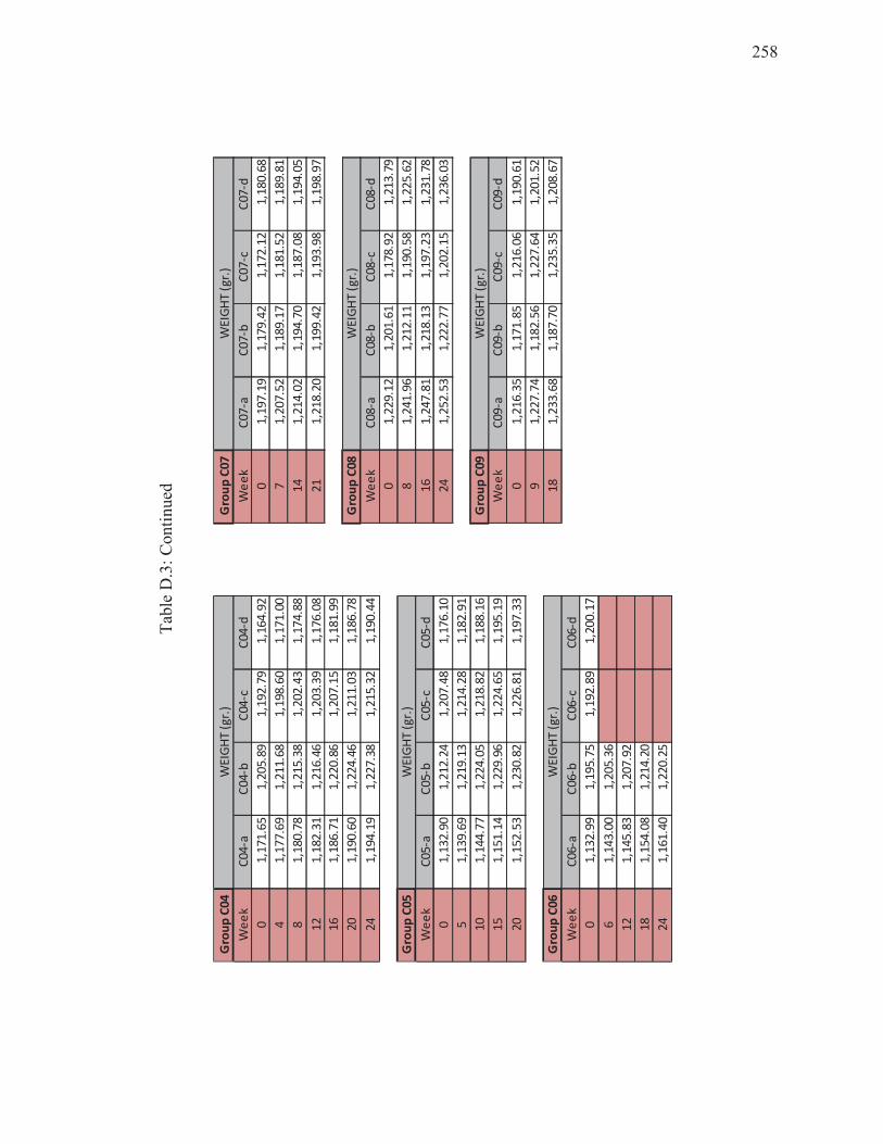
258
Tab
le D
.3:
Co
nti
nu
ed
Gro
up
C0
4G
rou
p C
07
We
ek
C0
4-a
C0
4-b
C04
-cC
04
-dW
ee
kC
07
-aC
07
-bC
07
-cC
07-d
01
,17
1.6
51
,20
5.8
91
,19
2.7
91
,16
4.9
20
1,1
97
.19
1,1
79
.42
1,1
72
.12
1,1
80.
68
41
,17
7.6
91
,21
1.6
81
,19
8.6
01
,17
1.0
07
1,2
07
.52
1,1
89
.17
1,1
81
.52
1,1
89.
81
81
,18
0.7
81
,21
5.3
81
,20
2.4
31
,17
4.8
81
41
,21
4.0
21
,19
4.7
01
,18
7.0
81
,19
4.0
5
12
1,1
82
.31
1,2
16
.46
1,2
03
.39
1,1
76
.08
21
1,2
18
.20
1,19
9.4
21
,19
3.9
81
,19
8.9
7
16
1,1
86
.71
1,2
20
.86
1,2
07
.15
1,1
81
.99
20
1,1
90
.60
1,2
24
.46
1,2
11
.03
1,1
86
.78
Gro
up
C0
8
24
1,1
94
.19
1,2
27
.38
1,2
15
.32
1,1
90
.44
We
ek
C0
8-a
C0
8-b
C0
8-c
C0
8-d
01
,22
9.1
21,
20
1.6
11
,17
8.9
21
,21
3.7
9
Gro
up
C0
58
1,2
41
.96
1,2
12
.11
1,1
90
.58
1,2
25
.62
We
ek
C0
5-a
C0
5-b
C05
-cC
05
-d1
61
,24
7.8
11,
21
8.1
31
,19
7.2
31
,23
1.7
8
01
,13
2.9
01
,21
2.2
41
,20
7.4
81
,17
6.1
02
41
,25
2.5
31
,22
2.7
71
,20
2.1
51
,23
6.0
3
51
,13
9.6
91
,21
9.1
31
,21
4.2
81
,18
2.9
1
10
1,1
44
.77
1,2
24
.05
1,2
18
.82
1,1
88
.16
Gro
up
C0
9
15
1,1
51
.14
1,2
29
.96
1,2
24
.65
1,1
95
.19
We
ek
C0
9-a
C0
9-b
C0
9-c
C0
9-d
20
1,1
52
.53
1,2
30
.82
1,2
26
.81
1,1
97
.33
01
,21
6.3
51,
171
.85
1,2
16
.06
1,1
90.
61
91
,22
7.7
41,
18
2.5
61
,22
7.6
41
,20
1.5
2
Gro
up
C0
61
81
,23
3.6
81
,18
7.7
01
,23
5.3
51
,20
8.6
7
We
ek
C0
6-a
C0
6-b
C06
-cC
06
-d
01
,13
2.9
91
,19
5.7
51
,19
2.8
91
,20
0.1
7
61
,14
3.0
01
,20
5.3
6
12
1,1
45
.83
1,2
07
.92
18
1,1
54
.08
1,2
14
.20
24
1,1
61
.40
1,2
20
.25
WE
IGH
T (
gr.
)
WE
IGH
T (
gr.
)
WE
IGH
T (
gr.
)
WE
IGH
T (
gr.
)
WE
IGH
T (
gr.
)
WE
IGH
T (
gr.
)
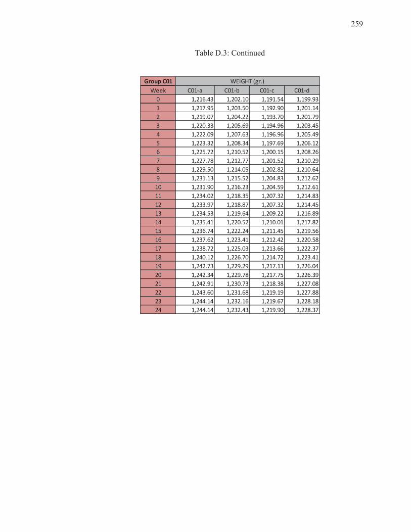
259
Table D.3: Continued
Group C01
Week C01-a C01-b C01-c C01-d
0 1,216.43 1,202.10 1,191.54 1,199.93
1 1,217.95 1,203.50 1,192.90 1,201.14
2 1,219.07 1,204.22 1,193.70 1,201.79
3 1,220.33 1,205.69 1,194.96 1,203.45
4 1,222.09 1,207.63 1,196.96 1,205.49
5 1,223.32 1,208.34 1,197.69 1,206.12
6 1,225.72 1,210.52 1,200.15 1,208.26
7 1,227.78 1,212.77 1,201.52 1,210.29
8 1,229.50 1,214.05 1,202.82 1,210.64
9 1,231.13 1,215.52 1,204.83 1,212.62
10 1,231.90 1,216.23 1,204.59 1,212.61
11 1,234.02 1,218.35 1,207.32 1,214.83
12 1,233.97 1,218.87 1,207.32 1,214.45
13 1,234.53 1,219.64 1,209.22 1,216.89
14 1,235.41 1,220.52 1,210.01 1,217.82
15 1,236.74 1,222.24 1,211.45 1,219.56
16 1,237.62 1,223.41 1,212.42 1,220.58
17 1,238.72 1,225.03 1,213.66 1,222.37
18 1,240.12 1,226.70 1,214.72 1,223.41
19 1,242.73 1,229.29 1,217.13 1,226.04
20 1,242.34 1,229.78 1,217.75 1,226.39
21 1,242.91 1,230.73 1,218.38 1,227.08
22 1,243.60 1,231.68 1,219.19 1,227.88
23 1,244.14 1,232.16 1,219.67 1,228.18
24 1,244.14 1,232.43 1,219.90 1,228.37
WEIGHT (gr.)
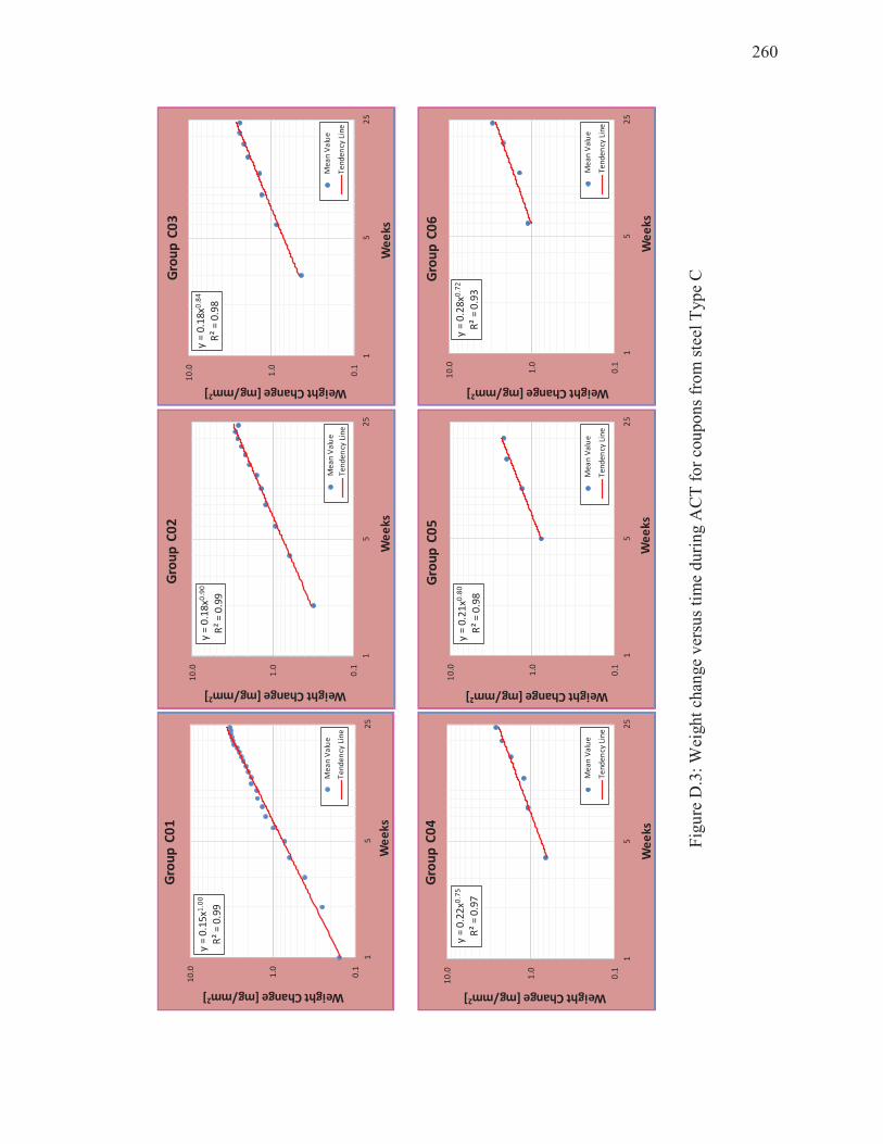
260
Fig
ure
D.3
: W
eigh
t ch
ange
ver
sus
tim
e d
uri
ng A
CT
fo
r co
up
on
s fr
om
ste
el T
yp
e C
y =
0.1
5x1
.00
R²
= 0
.99
0.1
1.0
10
.0
15
25
Weight Change [mg/mm2]
We
ek
s
Gro
up
C0
1
Me
an
Va
lue
Te
nd
en
cy L
ine
y =
0.1
8x0
.90
R²
= 0
.99
0.1
1.0
10
.0
15
25
Weight Change [mg/mm2]
We
ek
s
Gro
up
C0
2
Me
an
Va
lue
Te
nd
en
cy L
ine
y =
0.1
8x0
.84
R²
= 0
.98
0.1
1.0
10
.0
15
25
Weight Change [mg/mm2]
We
eks
Gro
up
C0
3
Me
an
Va
lue
Te
nd
en
cy L
ine
y =
0.2
2x0
.75
R²
= 0
.97
0.1
1.0
10
.0
15
25
Weight Change [mg/mm2]
We
ek
s
Gro
up
C0
4
Me
an
Va
lue
Te
nd
en
cy L
ine
y =
0.2
1x0
.80
R²
= 0
.98
0.1
1.0
10
.0
15
25
Weight Change [mg/mm2]
We
ek
s
Gro
up
C0
5
Me
an
Va
lue
Te
nd
en
cy L
ine
y =
0.2
8x0
.72
R²
= 0
.93
0.1
1.0
10
.0
15
25
Weight Change [mg/mm2]
We
ek
s
Gro
up
C0
6
Me
an
Va
lue
Te
nd
en
cy L
ine
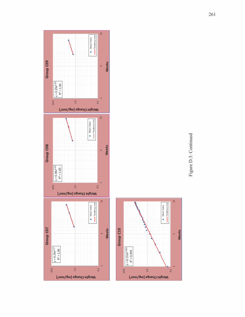
261
Fig
ure
D.3
: C
on
tin
ued
y =
0.2
9x0
.67
R²
= 1
.00
0.1
1.0
10
.0
15
25
Weight Change [mg/mm2]
We
eks
Gro
up
C0
7
Me
an
Va
lue
Te
nd
en
cy L
ine
y =
0.3
8x0
.60
R²
= 1
.00
0.1
1.0
10
.0
15
25
Weight Change [mg/mm2]
We
ek
s
Gro
up
C0
8
Me
an
Va
lue
Te
nd
en
cy L
ine
y =
0.2
9x0
.66
R²
= 1
.00
0.1
1.0
10
.0
15
25
Weight Change [mg/mm2]
We
ek
s
Gro
up
C0
9
Me
an
Va
lue
Te
nd
en
cy L
ine
y =
0.1
52
x0.9
83
R²
= 0
.99
3
0.1
1.0
10
.0
15
25
Weight Change [mg/mm2]
We
eks
Gro
up
C1
0
Me
an
Va
lue
Te
nd
en
cy L
ine
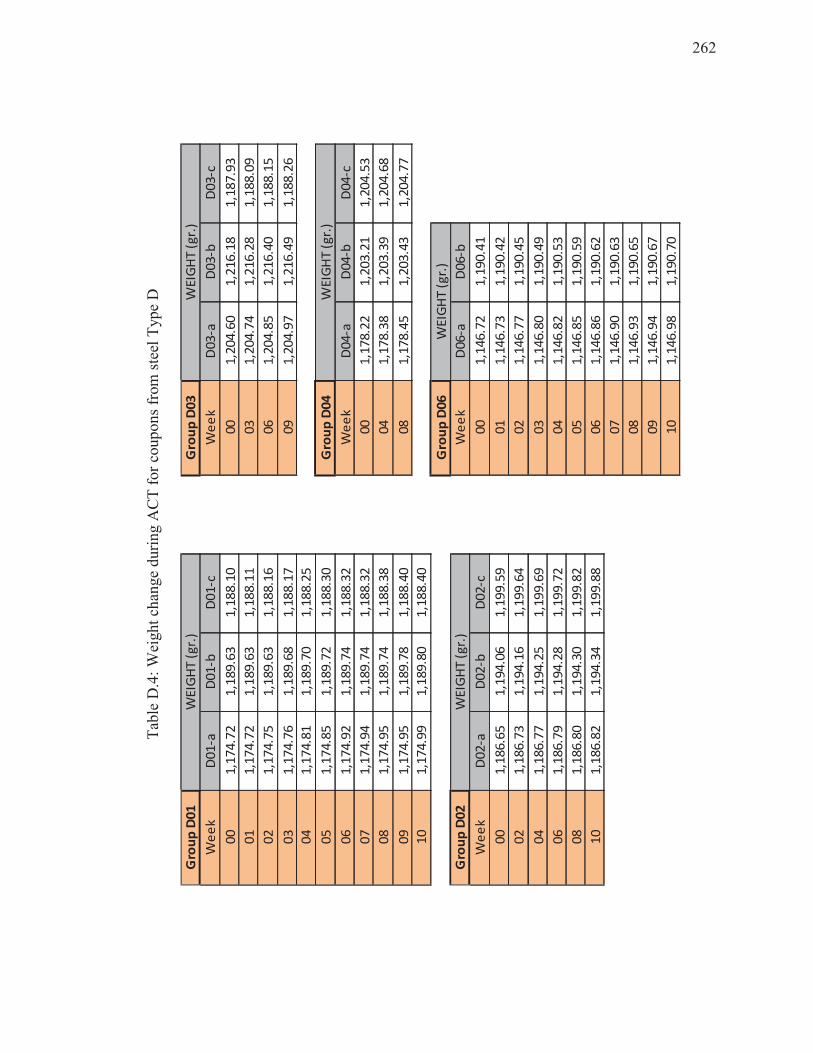
262
Tab
le D
.4:
Wei
gh
t ch
ang
e d
uri
ng A
CT
fo
r co
up
on
s fr
om
ste
el T
yp
e D
Gro
up
D0
1G
rou
p D
03
We
ek
D0
1-a
D0
1-b
D0
1-c
We
ek
D0
3-a
D0
3-b
D0
3-c
00
1,1
74
.72
1,1
89
.63
1,1
88
.10
00
1,2
04
.60
1,2
16
.18
1,1
87
.93
01
1,1
74
.72
1,1
89
.63
1,1
88
.11
03
1,2
04
.74
1,2
16
.28
1,1
88
.09
02
1,1
74
.75
1,1
89
.63
1,1
88
.16
06
1,2
04
.85
1,2
16
.40
1,1
88
.15
03
1,1
74
.76
1,1
89
.68
1,1
88
.17
09
1,2
04
.97
1,2
16
.49
1,1
88
.26
04
1,1
74
.81
1,1
89
.70
1,1
88
.25
05
1,1
74
.85
1,1
89
.72
1,1
88
.30
Gro
up
D0
4
06
1,1
74
.92
1,1
89
.74
1,1
88
.32
We
ek
D0
4-a
D0
4-b
D0
4-c
07
1,1
74
.94
1,1
89
.74
1,1
88
.32
00
1,1
78
.22
1,2
03
.21
1,2
04
.53
08
1,1
74
.95
1,1
89
.74
1,1
88
.38
04
1,1
78
.38
1,2
03
.39
1,2
04
.68
09
1,1
74
.95
1,1
89
.78
1,1
88
.40
08
1,1
78
.45
1,2
03
.43
1,2
04
.77
10
1,1
74
.99
1,1
89
.80
1,1
88
.40
Gro
up
D0
6
Gro
up
D0
2W
ee
kD
06
-aD
06
-b
We
ek
D0
2-a
D0
2-b
D0
2-c
00
1,1
46
.72
1,1
90
.41
00
1,1
86
.65
1,1
94
.06
1,1
99
.59
01
1,1
46
.73
1,1
90
.42
02
1,1
86
.73
1,1
94
.16
1,1
99
.64
02
1,1
46
.77
1,1
90
.45
04
1,1
86
.77
1,1
94
.25
1,1
99
.69
03
1,1
46
.80
1,1
90
.49
06
1,1
86
.79
1,1
94
.28
1,1
99
.72
04
1,1
46
.82
1,1
90
.53
08
1,1
86
.80
1,1
94
.30
1,1
99
.82
05
1,1
46
.85
1,1
90
.59
10
1,1
86
.82
1,1
94
.34
1,1
99
.88
06
1,1
46
.86
1,1
90
.62
07
1,1
46
.90
1,1
90
.63
08
1,1
46
.93
1,1
90
.65
09
1,1
46
.94
1,1
90
.67
10
1,1
46
.98
1,1
90
.70
WE
IGH
T (
gr.
)
WE
IGH
T (
gr.
)
WE
IGH
T (
gr.
)
WE
IGH
T (
gr.
)
WE
IGH
T (
gr.
)
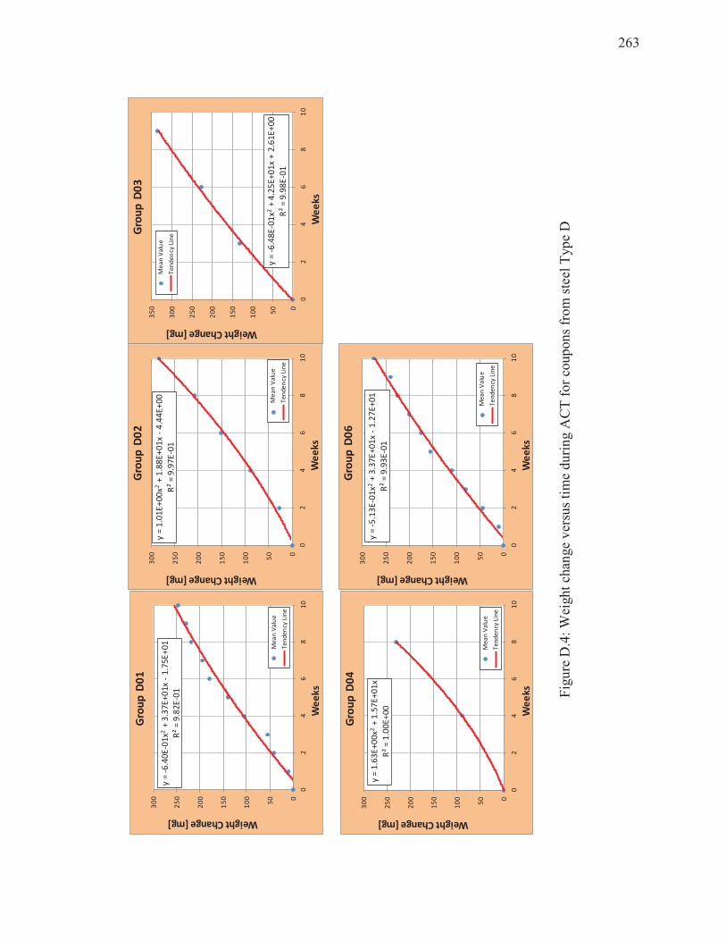
263
Fig
ure
D.4
: W
eigh
t ch
ange
ver
sus
tim
e d
uri
ng A
CT
fo
r co
up
on
s fr
om
ste
el T
yp
e D
y =
-6
.40
E-0
1x2
+ 3
.37
E+
01
x -
1.7
5E
+0
1
R²
= 9
.82
E-0
1
0
50
10
0
15
0
20
0
25
0
30
0
02
46
81
0
Weight Change [mg]
We
ek
s
Gro
up
D0
1
Me
an
Va
lue
Te
nd
en
cy L
ine
y =
1.0
1E
+0
0x2
+ 1
.88
E+
01
x -
4.4
4E
+0
0
R²
= 9
.97
E-0
1
0
50
10
0
15
0
20
0
25
0
30
0
02
46
81
0
Weight Change [mg]
We
ek
s
Gro
up
D0
2
Me
an
Va
lue
Te
nd
en
cy L
ine
y =
-6
.48
E-0
1x2
+ 4
.25
E+
01
x +
2.6
1E
+0
0
R²
= 9
.98
E-0
10
50
10
0
15
0
20
0
25
0
30
0
35
0
02
46
81
0
Weight Change [mg]
We
ek
s
Gro
up
D0
3
Me
an
Va
lue
Te
nd
en
cy L
ine
y =
1.6
3E
+0
0x2
+ 1
.57
E+
01
x
R²
= 1
.00
E+
00
0
50
10
0
15
0
20
0
25
0
30
0
02
46
81
0
Weight Change [mg]
We
ek
s
Gro
up
D0
4
Me
an
Va
lue
Te
nd
en
cy L
ine
y =
-5
.13
E-0
1x2
+ 3
.37
E+
01
x -
1.2
7E
+0
1
R²
= 9
.93
E-0
1
0
50
10
0
15
0
20
0
25
0
30
0
02
46
81
0
Weight Change [mg]
We
ek
s
Gro
up
D0
6
Me
an
Va
lue
Te
nd
en
cy L
ine

264
Appendix E Initial Dimensions of Coupons
The initial dimensions of each steel coupon are presented. The area for both faces, the
mean area and mean thickness are evaluated for each coupon. The data are presented in
tables for each steel type and each group (01 to 10).
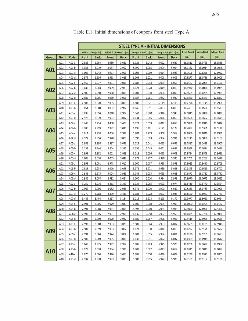
265
Table E.1: Initial dimensions of coupons from steel Type A
Group No. Code Front Back Front Back Front Back Front Back
A01 A01-a 2.983 2.994 2.980 3.021 6.025 6.042 6.022 6.027 18.0311 18.0765 18.0538
A02 A01-b 3.033 3.019 3.037 2.997 5.990 5.985 5.999 5.994 18.1182 18.0914 18.1048
A03 A01-c 3.006 3.042 2.957 2.966 6.002 6.009 6.014 6.023 18.1606 17.8238 17.9922
A04 A01-d 2.975 2.986 2.993 3.023 6.009 6.021 6.008 6.009 17.9277 18.0736 18.0006
A05 A02-a 2.959 2.977 2.981 3.018 6.088 6.054 6.084 6.053 18.0187 18.2025 18.1106
A06 A02-b 3.036 3.003 2.999 2.983 6.023 6.028 6.019 6.019 18.1940 18.0028 18.0984
A07 A02-c 2.986 2.998 2.988 3.018 6.001 6.010 6.004 6.003 17.9685 18.0285 17.9985
A08 A02-d 2.985 3.005 2.960 3.008 5.987 5.981 5.982 5.980 17.9221 17.8473 17.8847
A09 A03-a 2.983 3.020 2.985 3.006 6.108 6.071 6.119 6.109 18.2776 18.3145 18.2961
A10 A03-b 3.054 3.000 3.002 2.992 6.046 6.011 6.033 6.018 18.2483 18.0584 18.1533
A11 A03-c 3.035 2.994 3.010 2.987 5.942 5.988 5.916 5.945 17.9815 17.7826 17.8820
A12 A03-d 2.978 3.039 2.997 3.012 6.034 6.045 6.026 6.066 18.1698 18.1652 18.1675
A13 A04-a 3.248 3.214 3.450 3.408 6.023 6.053 6.012 6.058 19.5088 20.6940 20.1014
A14 A04-b 2.986 2.999 2.992 3.036 6.196 6.161 6.171 6.129 18.4892 18.5361 18.5126
A15 A04-c 3.014 2.974 3.006 2.987 5.982 5.979 5.968 5.969 17.9056 17.8846 17.8951
A16 A04-d 2.977 2.994 2.970 3.006 5.998 6.003 5.994 5.991 17.9145 17.9056 17.9100
A17 A05-a 2.982 2.998 2.987 3.033 6.025 6.041 6.023 6.032 18.0387 18.1428 18.0907
A18 A05-b 3.133 3.144 3.304 3.337 6.056 6.049 6.061 6.038 18.9958 20.0874 19.5416
A19 A05-c 2.999 2.982 3.001 2.968 6.013 6.006 6.023 6.009 17.9714 17.9548 17.9631
A20 A05-d 3.005 3.074 3.005 3.047 5.979 5.977 5.990 5.990 18.1701 18.1257 18.1479
A21 A06-a 2.993 3.001 2.973 3.012 6.000 6.007 5.998 5.998 17.9925 17.9490 17.9708
A22 A06-b 2.888 2.934 2.979 3.048 5.973 5.971 5.959 5.958 17.3845 17.9559 17.6702
A23 A06-c 2.983 2.975 3.024 2.985 6.043 6.033 6.068 6.028 17.9872 18.1712 18.0792
A24 A06-d 2.986 3.008 2.982 3.024 6.000 6.010 5.994 5.999 17.9970 18.0075 18.0022
A25 A07-a 3.250 3.216 3.413 3.391 6.024 6.065 6.023 6.074 19.5419 20.5770 20.0594
A26 A07-b 2.962 2.906 3.052 2.986 5.975 5.970 5.993 5.982 17.5233 18.0763 17.7998
A27 A07-c 3.270 3.288 3.399 3.441 6.083 6.028 6.063 6.038 19.8560 20.6927 20.2743
A28 A07-d 3.449 3.404 3.237 3.184 6.219 6.218 6.228 6.172 21.3077 19.9051 20.6064
A29 A08-a 2.991 3.005 2.979 3.033 6.000 6.008 5.995 5.998 18.0000 18.0255 18.0127
A30 A08-b 2.991 3.008 2.961 3.018 5.992 6.000 5.984 5.988 17.9850 17.8951 17.9401
A31 A08-c 2.993 3.005 2.951 2.998 6.035 5.998 5.997 5.953 18.0435 17.7726 17.9081
A32 A08-d 3.007 2.990 3.020 2.982 5.980 5.987 5.998 5.995 17.9415 17.9955 17.9685
A33 A09-a 2.993 3.000 2.983 3.026 5.989 6.004 5.993 6.002 17.9685 18.0195 17.9940
A34 A09-b 2.982 2.999 2.953 3.002 6.023 6.030 6.016 6.019 18.0222 17.9171 17.9697
A35 A09-c 2.991 3.004 2.974 3.004 6.003 6.015 5.994 6.001 18.0120 17.9265 17.9693
A36 A09-d 2.983 2.989 2.985 3.016 6.030 6.051 6.022 6.037 18.0369 18.0915 18.0642
A37 A10-a 3.048 2.975 2.992 2.957 5.985 5.983 5.975 5.973 18.0208 17.7697 17.8952
A38 A10-b 2.979 3.028 2.984 2.996 6.007 6.002 6.013 6.017 18.0345 17.9849 18.0097
A39 A10-c 2.970 3.004 2.976 3.010 6.085 6.050 6.046 6.007 18.1236 18.0373 18.0805
A40 A10-d 2.937 2.978 2.993 3.070 5.988 5.995 5.972 5.980 17.7199 18.1162 17.9181
A06
A07
A08
A09
A10
A01
A02
A03
A04
A05
Width 1 (Top) - [in] Width 2 (Bottom) - [in] Length 1 (Left) - [in] Length 2 (Right) - [in] Area Front
[in2]
STEEL TYPE A - INITIAL DIMENSIONSMean Area
[in2]
Area Back
[in2]
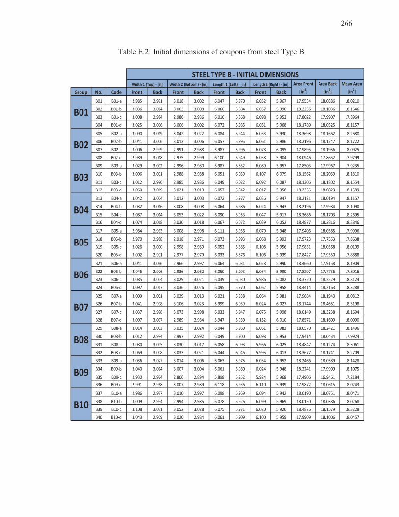
266
Table E.2: Initial dimensions of coupons from steel Type B
Group No. Code Front Back Front Back Front Back Front Back
B01 B01-a 2.985 2.991 3.018 3.002 6.047 5.970 6.052 5.967 17.9534 18.0886 18.0210
B02 B01-b 3.036 3.014 3.003 3.008 6.066 5.984 6.057 5.990 18.2256 18.1036 18.1646
B03 B01-c 3.008 2.984 2.986 2.986 6.016 5.868 6.098 5.952 17.8022 17.9907 17.8964
B04 B01-d 3.025 3.006 3.006 3.002 6.072 5.985 6.051 5.968 18.1789 18.0525 18.1157
B05 B02-a 3.090 3.019 3.042 3.022 6.084 5.944 6.053 5.930 18.3698 18.1662 18.2680
B06 B02-b 3.041 3.006 3.012 3.006 6.057 5.995 6.061 5.986 18.2196 18.1247 18.1722
B07 B02-c 3.006 2.999 2.991 2.988 5.987 5.996 6.078 6.095 17.9895 18.1956 18.0925
B08 B02-d 2.989 3.018 2.975 2.999 6.100 5.949 6.058 5.904 18.0946 17.8652 17.9799
B09 B03-a 3.029 3.002 2.996 2.980 5.987 5.852 6.089 5.957 17.8503 17.9967 17.9235
B10 B03-b 3.006 3.001 2.988 2.988 6.051 6.039 6.107 6.079 18.1562 18.2059 18.1810
B11 B03-c 3.012 2.996 2.985 2.986 6.049 6.022 6.092 6.087 18.1306 18.1802 18.1554
B12 B03-d 3.060 3.019 3.021 3.019 6.057 5.942 6.017 5.958 18.2355 18.0823 18.1589
B13 B04-a 3.042 3.004 3.012 3.003 6.072 5.977 6.036 5.947 18.2121 18.0194 18.1157
B14 B04-b 3.032 3.016 3.008 3.008 6.064 5.986 6.024 5.943 18.2196 17.9984 18.1090
B15 B04-c 3.087 3.014 3.053 3.022 6.090 5.953 6.047 5.917 18.3686 18.1703 18.2695
B16 B04-d 3.074 3.018 3.030 3.018 6.067 6.072 6.039 6.052 18.4877 18.2816 18.3846
B17 B05-a 2.984 2.963 3.008 2.998 6.111 5.956 6.079 5.948 17.9406 18.0585 17.9996
B18 B05-b 2.970 2.988 2.918 2.971 6.073 5.993 6.068 5.992 17.9723 17.7553 17.8638
B19 B05-c 3.026 3.000 2.998 2.989 6.052 5.885 6.108 5.956 17.9831 18.0568 18.0199
B20 B05-d 3.002 2.991 2.977 2.979 6.033 5.876 6.106 5.939 17.8427 17.9350 17.8888
B21 B06-a 3.041 3.066 2.966 2.997 6.064 6.031 6.028 5.990 18.4660 17.9158 18.1909
B22 B06-b 2.946 2.976 2.936 2.962 6.050 5.993 6.064 5.990 17.8297 17.7736 17.8016
B23 B06-c 3.085 3.004 3.029 3.021 6.039 6.030 5.986 6.082 18.3720 18.2529 18.3124
B24 B06-d 3.097 3.017 3.036 3.026 6.095 5.970 6.062 5.958 18.4414 18.2163 18.3288
B25 B07-a 3.009 3.001 3.029 3.013 6.021 5.938 6.064 5.981 17.9684 18.1940 18.0812
B26 B07-b 3.041 2.998 3.106 3.023 5.999 6.039 6.024 6.027 18.1744 18.4651 18.3198
B27 B07-c 3.037 2.978 3.073 2.998 6.033 5.947 6.075 5.998 18.0149 18.3238 18.1694
B28 B07-d 3.007 3.007 2.989 2.984 5.947 5.930 6.152 6.010 17.8571 18.1609 18.0090
B29 B08-a 3.014 3.003 3.035 3.024 6.044 5.960 6.061 5.982 18.0570 18.2421 18.1496
B30 B08-b 3.012 2.994 2.997 2.992 6.049 5.900 6.098 5.953 17.9414 18.0434 17.9924
B31 B08-c 3.080 3.005 3.030 3.017 6.058 6.093 5.966 6.025 18.4847 18.1274 18.3061
B32 B08-d 3.069 3.008 3.033 3.021 6.044 6.046 5.995 6.013 18.3677 18.1741 18.2709
B33 B09-a 3.036 3.027 3.014 3.006 6.063 5.975 6.034 5.952 18.2466 18.0389 18.1428
B34 B09-b 3.040 3.014 3.007 3.004 6.061 5.980 6.024 5.948 18.2241 17.9909 18.1075
B35 B09-c 2.930 2.974 2.806 2.894 5.898 5.952 5.924 5.968 17.4906 16.9461 17.2184
B36 B09-d 2.991 2.968 3.007 2.989 6.118 5.956 6.110 5.939 17.9872 18.0615 18.0243
B37 B10-a 2.986 2.987 3.010 2.997 6.098 5.969 6.094 5.942 18.0190 18.0751 18.0471
B38 B10-b 3.009 2.994 2.994 2.985 6.078 5.926 6.099 5.969 18.0150 18.0386 18.0268
B39 B10-c 3.108 3.031 3.052 3.028 6.075 5.971 6.020 5.926 18.4876 18.1579 18.3228
B40 B10-d 3.043 2.969 3.020 2.984 6.061 5.909 6.100 5.959 17.9909 18.1006 18.0457
B06
B07
B08
B09
B10
B01
B02
B03
B04
B05
Width 1 (Top) - [in] Width 2 (Bottom) - [in] Length 1 (Left) - [in] Length 2 (Right) - [in] Area Front
[in2]
Area Back
[in2]
Mean Area
[in2]
STEEL TYPE B - INITIAL DIMENSIONS
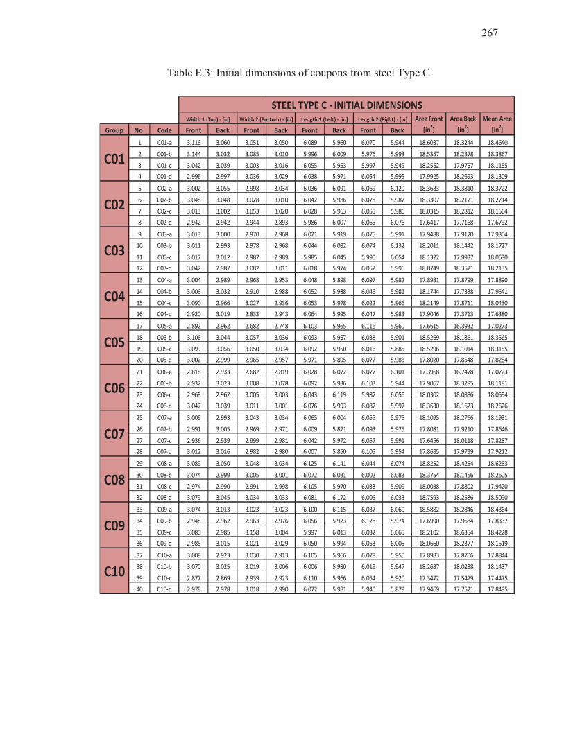
267
Table E.3: Initial dimensions of coupons from steel Type C
Group No. Code Front Back Front Back Front Back Front Back
1 C01-a 3.116 3.060 3.051 3.050 6.089 5.960 6.070 5.944 18.6037 18.3244 18.4640
2 C01-b 3.144 3.032 3.085 3.010 5.996 6.009 5.976 5.993 18.5357 18.2378 18.3867
3 C01-c 3.042 3.039 3.003 3.016 6.055 5.953 5.997 5.949 18.2552 17.9757 18.1155
4 C01-d 2.996 2.997 3.036 3.029 6.038 5.971 6.054 5.995 17.9925 18.2693 18.1309
5 C02-a 3.002 3.055 2.998 3.034 6.036 6.091 6.069 6.120 18.3633 18.3810 18.3722
6 C02-b 3.048 3.048 3.028 3.010 6.042 5.986 6.078 5.987 18.3307 18.2121 18.2714
7 C02-c 3.013 3.002 3.053 3.020 6.028 5.963 6.055 5.986 18.0315 18.2812 18.1564
8 C02-d 2.942 2.942 2.944 2.893 5.986 6.007 6.065 6.076 17.6417 17.7168 17.6792
9 C03-a 3.013 3.000 2.970 2.968 6.021 5.919 6.075 5.991 17.9488 17.9120 17.9304
10 C03-b 3.011 2.993 2.978 2.968 6.044 6.082 6.074 6.132 18.2011 18.1442 18.1727
11 C03-c 3.017 3.012 2.987 2.989 5.985 6.045 5.990 6.054 18.1322 17.9937 18.0630
12 C03-d 3.042 2.987 3.082 3.011 6.018 5.974 6.052 5.996 18.0749 18.3521 18.2135
13 C04-a 3.004 2.989 2.968 2.953 6.048 5.898 6.097 5.982 17.8981 17.8799 17.8890
14 C04-b 3.006 3.032 2.910 2.988 6.052 5.988 6.046 5.981 18.1744 17.7338 17.9541
15 C04-c 3.090 2.966 3.027 2.936 6.053 5.978 6.022 5.966 18.2149 17.8711 18.0430
16 C04-d 2.920 3.019 2.833 2.943 6.064 5.995 6.047 5.983 17.9046 17.3713 17.6380
17 C05-a 2.892 2.962 2.682 2.748 6.103 5.965 6.116 5.960 17.6615 16.3932 17.0273
18 C05-b 3.106 3.044 3.057 3.036 6.093 5.957 6.038 5.901 18.5269 18.1861 18.3565
19 C05-c 3.099 3.056 3.050 3.034 6.092 5.950 6.016 5.885 18.5296 18.1014 18.3155
20 C05-d 3.002 2.999 2.965 2.957 5.971 5.895 6.077 5.983 17.8020 17.8548 17.8284
21 C06-a 2.818 2.933 2.682 2.819 6.028 6.072 6.077 6.101 17.3968 16.7478 17.0723
22 C06-b 2.932 3.023 3.008 3.078 6.092 5.936 6.103 5.944 17.9067 18.3295 18.1181
23 C06-c 2.968 2.962 3.005 3.003 6.043 6.119 5.987 6.056 18.0302 18.0886 18.0594
24 C06-d 3.047 3.039 3.011 3.001 6.076 5.993 6.087 5.997 18.3630 18.1623 18.2626
25 C07-a 3.009 2.993 3.043 3.034 6.065 6.004 6.055 5.975 18.1095 18.2766 18.1931
26 C07-b 2.991 3.005 2.969 2.971 6.009 5.871 6.093 5.975 17.8081 17.9210 17.8646
27 C07-c 2.936 2.939 2.999 2.981 6.042 5.972 6.057 5.991 17.6456 18.0118 17.8287
28 C07-d 3.012 3.016 2.982 2.980 6.007 5.850 6.105 5.954 17.8685 17.9739 17.9212
29 C08-a 3.089 3.050 3.048 3.034 6.125 6.141 6.044 6.074 18.8252 18.4254 18.6253
30 C08-b 3.074 2.999 3.005 3.001 6.072 6.031 6.002 6.083 18.3754 18.1456 18.2605
31 C08-c 2.974 2.990 2.991 2.998 6.105 5.970 6.033 5.909 18.0038 17.8802 17.9420
32 C08-d 3.079 3.045 3.034 3.033 6.081 6.172 6.005 6.033 18.7593 18.2586 18.5090
33 C09-a 3.074 3.013 3.023 3.023 6.100 6.115 6.037 6.060 18.5882 18.2846 18.4364
34 C09-b 2.948 2.962 2.963 2.976 6.056 5.923 6.128 5.974 17.6990 17.9684 17.8337
35 C09-c 3.080 2.985 3.158 3.004 5.997 6.013 6.032 6.065 18.2102 18.6354 18.4228
36 C09-d 2.985 3.015 3.021 3.029 6.050 5.994 6.053 6.005 18.0660 18.2377 18.1519
37 C10-a 3.008 2.923 3.030 2.913 6.105 5.966 6.078 5.950 17.8983 17.8706 17.8844
38 C10-b 3.070 3.025 3.019 3.006 6.006 5.980 6.019 5.947 18.2637 18.0238 18.1437
39 C10-c 2.877 2.869 2.939 2.923 6.110 5.966 6.054 5.920 17.3472 17.5479 17.4475
40 C10-d 2.978 2.978 3.018 2.990 6.072 5.981 5.940 5.879 17.9469 17.7521 17.8495
C06
C07
C08
C09
C10
C01
C02
C03
C04
C05
Width 1 (Top) - [in] Width 2 (Bottom) - [in] Length 1 (Left) - [in] Length 2 (Right) - [in]
STEEL TYPE C - INITIAL DIMENSIONSArea Front
[in2]
Area Back
[in2]
Mean Area
[in2]

268
Appendix F Thickness Change During ACT
The thickness change for each steel coupon is presented in this Appendix, in tabulated
and graphical manner. Weight changes for coupons from steel Types A, B, and C are
presented week by week for the 24 weeks the ACT lasted. The data are presented for
each steel type and for each group, every week a group was subjected to washing.

269
Tab
le F
.1:
Thic
kn
ess
chan
ge
du
rin
g A
CT
fo
r co
up
on
s fr
om
ste
el T
yp
e A
Gro
up
A0
1G
rou
p A
02
We
ek
A0
1-a
A0
1-b
A0
1-c
A0
1-d
We
ek
A0
2-a
A0
2-b
A0
2-c
A0
2-d
00
.53
27
0.5
32
80
.53
13
0.5
32
00
0.5
30
10
.54
26
0.5
37
20
.53
59
10
.54
08
0.5
38
60
.53
97
0.5
39
52
0.5
43
60
.55
36
0.5
50
40
.54
76
20
.54
58
0.5
41
90
.54
53
0.5
43
64
0.5
53
00
.56
80
0.5
52
70
.55
54
30
.55
01
0.5
45
50
.54
96
0.5
50
26
0.5
68
40
.57
42
0.5
61
30
.56
90
40
.55
39
0.5
48
30
.55
28
0.5
50
18
0.5
71
60
.58
66
0.5
69
40
.57
79
50
.55
83
0.5
54
60
.55
76
0.5
54
91
00
.57
77
0.5
90
30
.57
34
0.5
88
4
60
.56
12
0.5
57
90
.56
12
0.5
58
81
20
.58
70
0.5
97
20
.58
06
0.5
93
2
70
.56
49
0.5
61
80
.56
28
0.5
60
41
40
.59
36
0.5
99
20
.58
61
0.5
98
3
80
.56
69
0.5
65
90
.56
46
0.5
62
21
60
.59
93
0.6
03
60
.59
33
0.6
03
9
90
.56
92
0.5
71
30
.57
03
0.5
65
01
80
.60
34
0.6
08
50
.59
69
0.6
07
6
10
0.5
70
20
.57
52
0.5
71
10
.56
81
20
0.6
04
40
.61
07
0.6
02
40
.61
06
11
0.5
72
00
.57
83
0.5
73
30
.57
09
22
0.6
06
60
.61
56
0.6
05
80
.61
36
12
0.5
76
70
.58
43
0.5
75
10
.57
44
24
0.6
12
30
.61
79
0.6
07
20
.61
45
13
0.5
79
10
.58
99
0.5
77
30
.57
78
14
0.5
81
80
.59
03
0.5
78
50
.57
74
Gro
up
A0
3
15
0.5
83
30
.59
31
0.5
80
40
.57
93
We
ek
A0
3-a
A0
3-b
A0
3-c
A0
3-d
16
0.5
84
40
.59
51
0.5
83
00
.58
05
00
.54
16
0.5
32
30
.53
22
0.5
39
7
17
0.5
86
80
.59
75
0.5
86
50
.58
26
30
.55
63
0.5
48
20
.54
63
0.5
53
3
18
0.5
89
20
.60
17
0.5
84
90
.58
26
60
.57
23
0.5
53
60
.56
49
0.5
62
1
19
0.5
90
50
.60
25
0.5
87
70
.58
49
90
.57
59
0.5
65
30
.56
97
0.5
68
8
20
0.5
92
60
.60
32
0.5
89
60
.58
65
12
0.5
83
90
.57
04
0.5
74
00
.57
61
21
0.5
95
50
.60
35
0.5
91
90
.59
12
15
0.5
88
70
.57
48
0.5
77
20
.57
93
22
0.5
97
10
.60
47
0.5
93
30
.59
39
18
0.5
90
90
.58
03
0.5
77
80
.58
50
23
0.5
98
50
.60
58
0.5
94
80
.59
51
21
0.5
96
00
.58
76
0.5
80
80
.58
81
24
0.5
99
80
.60
70
0.5
96
60
.59
73
24
0.6
01
10
.59
21
0.5
88
30
.59
34
TH
ICK
NE
SS
(in
.)T
HIC
KN
ES
S (
in.)
TH
ICK
NE
SS
(in
.)
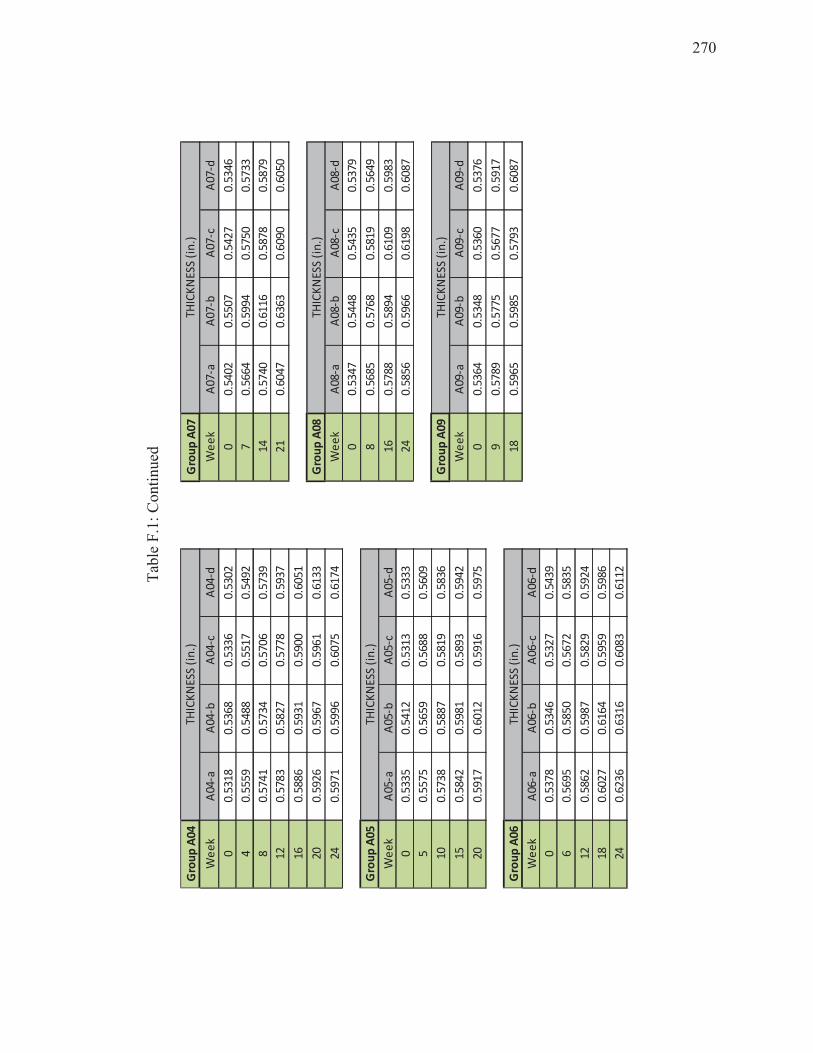
270
Tab
le F
.1:
Co
nti
nu
ed
Gro
up
A0
4G
rou
p A
07
We
ek
A04
-aA
04-b
A04
-cA
04-d
We
ek
A07
-aA
07-
bA
07-c
A07
-d
00.
531
80.
536
80
.533
60
.530
20
0.5
402
0.5
507
0.5
427
0.5
346
40.
555
90.
548
80
.551
70
.549
27
0.5
664
0.5
994
0.5
750
0.5
733
80.
574
10.
573
40
.570
60
.573
91
40
.57
400
.61
160
.587
80
.58
79
120.
578
30
.58
27
0.5
778
0.5
937
21
0.6
047
0.6
363
0.6
090
0.6
050
160.
588
60
.59
31
0.5
900
0.6
051
200.
592
60
.59
67
0.5
961
0.6
133
Gro
up
A0
8
240.
597
10
.59
96
0.6
075
0.6
174
We
ek
A08
-aA
08-
bA
08-c
A08
-d
00
.53
470
.544
80
.543
50
.53
79
Gro
up
A0
58
0.5
685
0.5
768
0.5
819
0.5
649
We
ek
A05
-aA
05-b
A05
-cA
05-d
16
0.5
788
0.5
894
0.6
109
0.5
983
00.
533
50.
541
20
.531
30
.533
32
40
.58
560
.59
660
.619
80
.60
87
50.
557
50.
565
90
.568
80
.560
9
100.
573
80
.58
87
0.5
819
0.5
836
Gro
up
A0
9
150.
584
20
.59
81
0.5
893
0.5
942
We
ek
A09
-aA
09-
bA
09-c
A09
-d
200.
591
70
.60
12
0.5
916
0.5
975
00
.53
640
.534
80
.536
00
.53
76
90
.57
890
.577
50
.567
70
.59
17
Gro
up
A0
618
0.5
965
0.5
985
0.5
793
0.6
087
We
ek
A06
-aA
06-b
A06
-cA
06-d
00.
537
80.
534
60
.532
70
.543
9
60.
569
50.
585
00
.567
20
.583
5
120.
586
20
.59
87
0.5
829
0.5
924
180.
602
70
.61
64
0.5
959
0.5
986
240.
623
60
.63
16
0.6
083
0.6
112
THIC
KN
ESS
(in
.)
THIC
KN
ESS
(in
.)
THIC
KN
ESS
(in
.)
THIC
KN
ESS
(in
.)
THIC
KN
ESS
(in
.)
THIC
KN
ESS
(in
.)
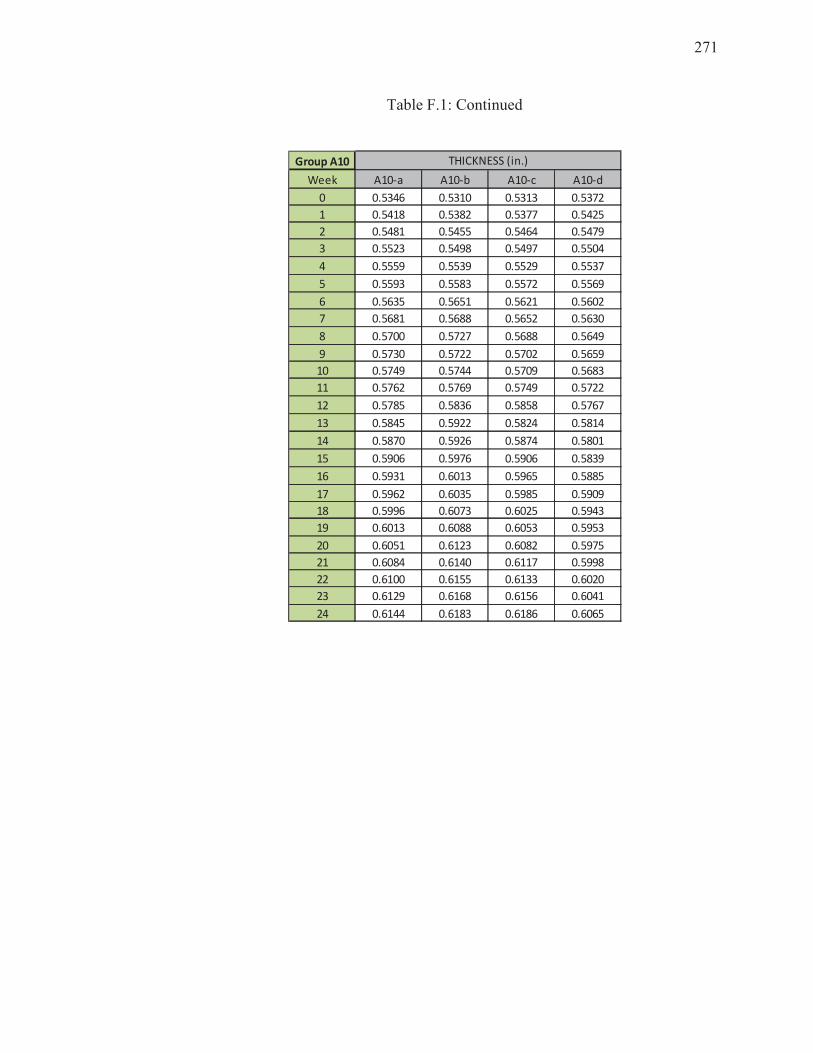
271
Table F.1: Continued
Group A10
Week A10-a A10-b A10-c A10-d
0 0.5346 0.5310 0.5313 0.5372
1 0.5418 0.5382 0.5377 0.5425
2 0.5481 0.5455 0.5464 0.5479
3 0.5523 0.5498 0.5497 0.5504
4 0.5559 0.5539 0.5529 0.5537
5 0.5593 0.5583 0.5572 0.5569
6 0.5635 0.5651 0.5621 0.5602
7 0.5681 0.5688 0.5652 0.5630
8 0.5700 0.5727 0.5688 0.5649
9 0.5730 0.5722 0.5702 0.5659
10 0.5749 0.5744 0.5709 0.5683
11 0.5762 0.5769 0.5749 0.5722
12 0.5785 0.5836 0.5858 0.5767
13 0.5845 0.5922 0.5824 0.5814
14 0.5870 0.5926 0.5874 0.5801
15 0.5906 0.5976 0.5906 0.5839
16 0.5931 0.6013 0.5965 0.5885
17 0.5962 0.6035 0.5985 0.5909
18 0.5996 0.6073 0.6025 0.5943
19 0.6013 0.6088 0.6053 0.5953
20 0.6051 0.6123 0.6082 0.5975
21 0.6084 0.6140 0.6117 0.5998
22 0.6100 0.6155 0.6133 0.6020
23 0.6129 0.6168 0.6156 0.6041
24 0.6144 0.6183 0.6186 0.6065
THICKNESS (in.)
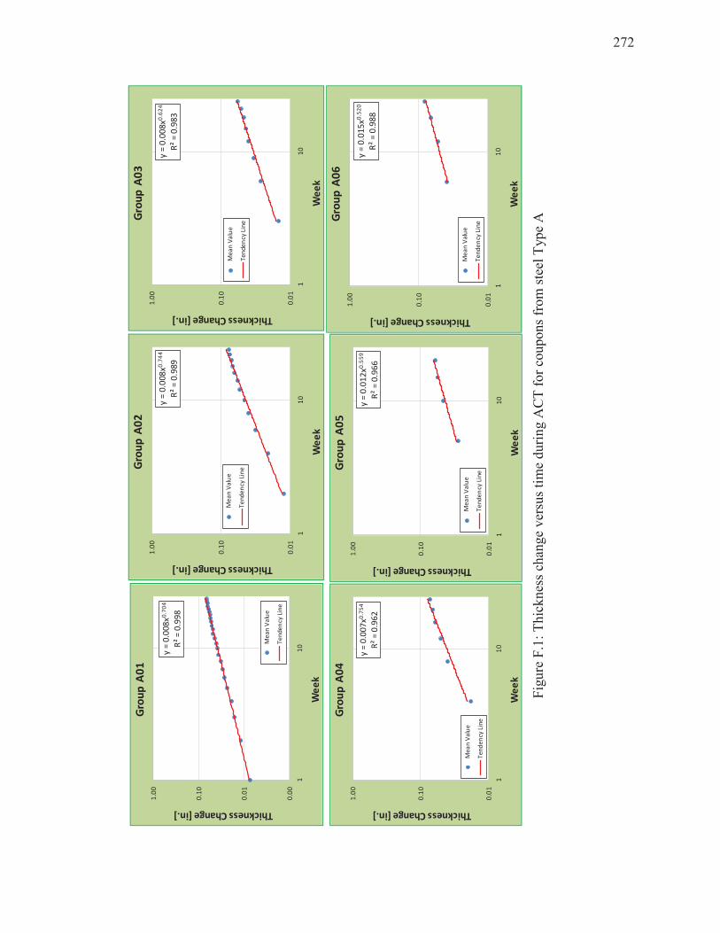
272
Fig
ure
F.1
: T
hic
kn
ess
chan
ge
ver
sus
tim
e d
uri
ng A
CT
fo
r co
up
on
s fr
om
ste
el T
yp
e A
y
= 0
.00
8x0
.70
4
R²
= 0
.99
8
0.0
0
0.0
1
0.1
0
1.0
0
11
0
Thickness Change [in.]
We
ek
Gro
up
A0
1
Me
an
Va
lue
Te
nd
en
cy L
ine
y =
0.0
08
x0.7
44
R²
= 0
.98
9
0.0
1
0.1
0
1.0
0
11
0
Thickness Change [in.]
We
ek
Gro
up
A0
2
Me
an
Va
lue
Te
nd
en
cy L
ine
y =
0.0
08
x0.6
24
R²
= 0
.98
3
0.0
1
0.1
0
1.0
0
11
0
Thickness Change [in.]
We
ek
Gro
up
A0
3
Me
an
Va
lue
Te
nd
en
cy L
ine
y =
0.0
07
x0.7
54
R²
= 0
.96
2
0.0
1
0.1
0
1.0
0
11
0
Thickness Change [in.]
We
ek
Gro
up
A0
4
Me
an
Va
lue
Te
nd
en
cy L
ine
y =
0.0
12
x0.5
59
R²
= 0
.96
6
0.0
1
0.1
0
1.0
0
11
0
Thickness Change [in.]
We
ek
Gro
up
A0
5
Me
an
Va
lue
Te
nd
en
cy L
ine
y =
0.0
15
x0.5
20
R²
= 0
.98
8
0.0
1
0.1
0
1.0
0
11
0
Thickness Change [in.]
We
ek
Gro
up
A0
6
Me
an
Va
lue
Te
nd
en
cy L
ine
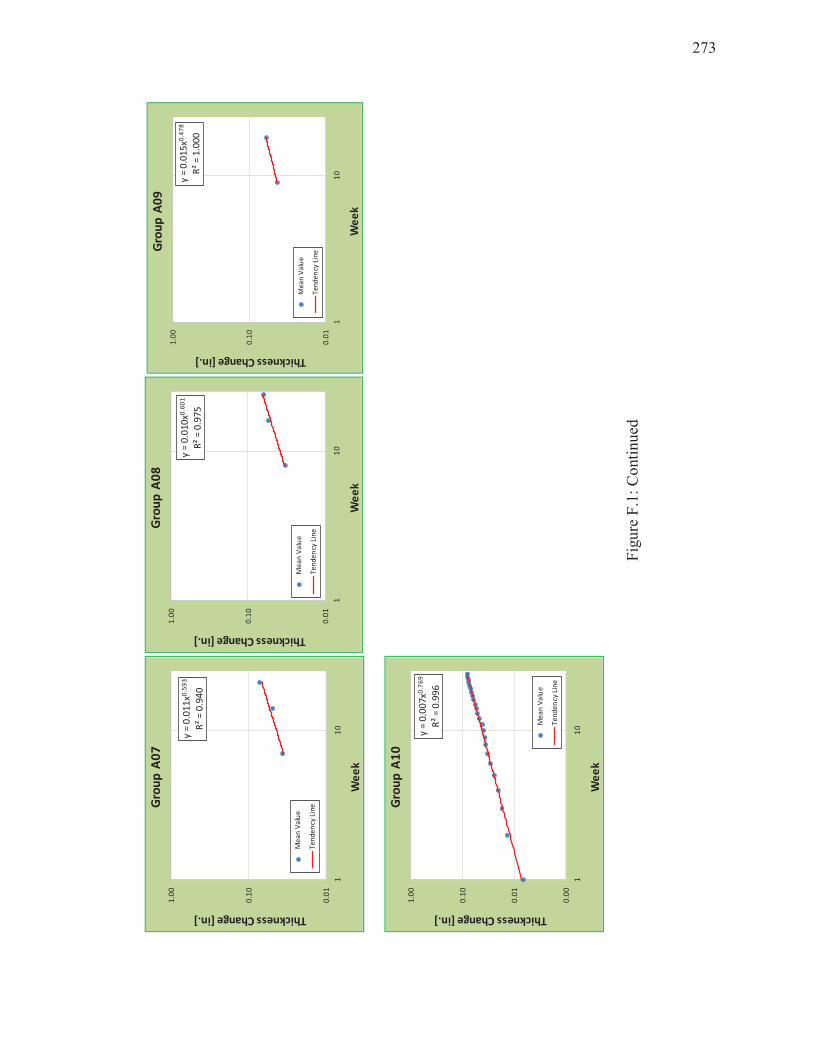
273
F
igu
re F
.1:
Co
nti
nu
ed
y =
0.0
11
x0.5
93
R²
= 0
.94
0
0.0
1
0.1
0
1.0
0
11
0
Thickness Change [in.]
We
ek
Gro
up
A0
7
Me
an
Va
lue
Te
nd
en
cy L
ine
y =
0.0
10
x0.6
01
R²
= 0
.97
5
0.0
1
0.1
0
1.0
0
11
0
Thickness Change [in.]
We
ek
Gro
up
A0
8
Me
an
Va
lue
Te
nd
en
cy L
ine
y =
0.0
15
x0.4
78
R²
= 1
.00
0
0.0
1
0.1
0
1.0
0
11
0
Thickness Change [in.]
We
ek
Gro
up
A0
9
Me
an
Va
lue
Te
nd
en
cy L
ine
y =
0.0
07
x0.7
69
R²
= 0
.99
6
0.0
0
0.0
1
0.1
0
1.0
0
11
0
Thickness Change [in.]
We
ek
Gro
up
A1
0
Me
an
Va
lue
Te
nd
en
cy L
ine
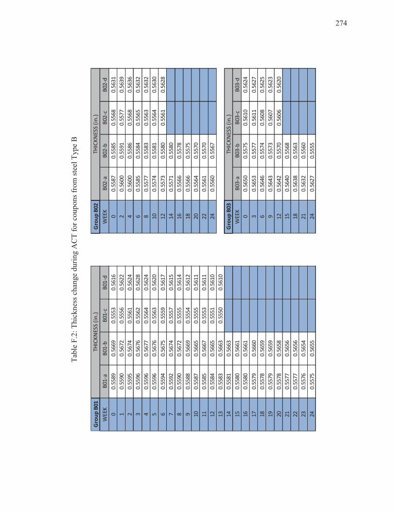
274
Tab
le F
.2:
Thic
kn
ess
chan
ge
du
rin
g A
CT
fo
r co
up
on
s fr
om
ste
el T
yp
e B
Gro
up
B0
1G
rou
p B
02
WE
EK
B0
1-a
B0
1-b
B0
1-c
B0
1-d
WE
EK
B0
2-a
B0
2-b
B0
2-c
B0
2-d
00
.55
89
0.5
66
90
.55
53
0.5
61
60
0.5
58
70
.55
85
0.5
56
80
.56
31
10
.55
90
0.5
67
20
.55
56
0.5
62
22
0.5
60
00
.55
91
0.5
57
70
.56
39
20
.55
95
0.5
67
40
.55
61
0.5
62
44
0.5
60
00
.55
86
0.5
56
80
.56
36
30
.55
96
0.5
67
60
.55
62
0.5
62
86
0.5
58
50
.55
84
0.5
56
50
.56
32
40
.55
96
0.5
67
70
.55
64
0.5
62
48
0.5
57
70
.55
83
0.5
56
30
.56
32
50
.55
96
0.5
67
60
.55
63
0.5
62
01
00
.55
74
0.5
58
10
.55
64
0.5
63
0
60
.55
94
0.5
67
50
.55
59
0.5
61
71
20
.55
73
0.5
58
00
.55
61
0.5
62
8
70
.55
92
0.5
67
40
.55
57
0.5
61
51
40
.55
71
0.5
58
0
80
.55
90
0.5
67
20
.55
55
0.5
61
41
60
.55
66
0.5
57
8
90
.55
88
0.5
66
90
.55
54
0.5
61
21
80
.55
66
0.5
57
5
10
0.5
58
70
.56
65
0.5
55
50
.56
11
20
0.5
56
40
.55
70
11
0.5
58
50
.56
67
0.5
55
30
.56
11
22
0.5
56
10
.55
70
12
0.5
58
40
.56
65
0.5
55
10
.56
10
24
0.5
56
00
.55
67
13
0.5
58
30
.56
63
0.5
55
00
.56
10
14
0.5
58
10
.56
63
Gro
up
B0
3
15
0.5
58
00
.56
61
WE
EK
B0
3-a
B0
3-b
B0
3-c
B0
3-d
16
0.5
58
00
.56
61
00
.56
50
0.5
57
50
.56
10
0.5
62
4
17
0.5
57
90
.56
60
30
.56
53
0.5
57
70
.56
11
0.5
62
7
18
0.5
57
80
.56
59
60
.56
46
0.5
57
40
.56
08
0.5
62
5
19
0.5
57
90
.56
59
90
.56
43
0.5
57
30
.56
07
0.5
62
3
20
0.5
57
80
.56
58
12
0.5
64
20
.55
70
0.5
60
60
.56
20
21
0.5
57
70
.56
56
15
0.5
64
00
.55
68
22
0.5
57
70
.56
56
18
0.5
63
80
.55
63
23
0.5
57
60
.56
54
21
0.5
63
20
.55
60
24
0.5
57
50
.56
55
24
0.5
62
70
.55
55
TH
ICK
NE
SS
(in
.)
TH
ICK
NE
SS
(in
.)
TH
ICK
NE
SS
(in
.)
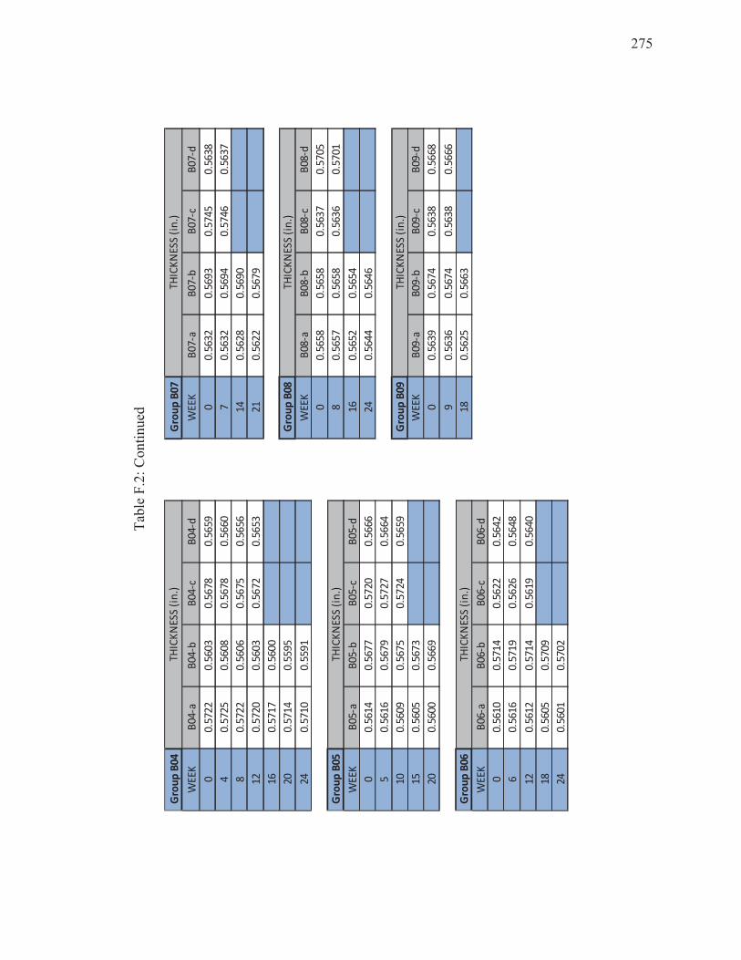
275
Tab
le F
.2:
Co
nti
nu
ed
Gro
up
B04
Gro
up
B0
7
WEE
KB
04-a
B04
-bB
04-c
B04
-dW
EEK
B07
-aB
07-b
B07
-cB
07-d
00.
5722
0.56
03
0.5
678
0.56
590
0.56
320.
569
30
.574
50
.56
38
40.
5725
0.56
08
0.5
678
0.56
607
0.56
320.
569
40
.574
60
.56
37
80.
5722
0.56
06
0.5
675
0.56
5614
0.56
280.
569
0
120.
5720
0.56
03
0.5
672
0.56
5321
0.56
220.
567
9
160.
5717
0.56
00
200.
5714
0.55
95
Gro
up
B08
240.
5710
0.55
91
WEE
KB
08-a
B0
8-b
B08
-cB
08-d
00.
5658
0.56
58
0.5
637
0.5
705
Gro
up
B05
80.
5657
0.56
58
0.5
636
0.5
701
WEE
KB
05-a
B05
-bB
05-c
B05
-d16
0.56
520.
565
4
00.
5614
0.56
77
0.5
720
0.56
6624
0.56
440.
564
6
50.
5616
0.56
79
0.5
727
0.56
64
100.
5609
0.56
75
0.5
724
0.56
59G
rou
p B
09
150.
5605
0.56
73
WEE
KB
09-a
B0
9-b
B09
-cB
09-d
200.
5600
0.56
69
00.
5639
0.56
74
0.5
638
0.5
668
90.
5636
0.56
74
0.5
638
0.5
666
Gro
up
B06
180.
5625
0.56
63
WEE
KB
06-a
B06
-bB
06-c
B06
-d
00.
5610
0.57
14
0.5
622
0.56
42
60.
5616
0.57
19
0.5
626
0.56
48
120.
5612
0.57
14
0.5
619
0.56
40
180.
5605
0.57
09
240.
5601
0.57
02
THIC
KN
ESS
(in
.)
THIC
KN
ESS
(in
.)
THIC
KN
ESS
(in
.)
THIC
KN
ESS
(in
.)
THIC
KN
ESS
(in
.)
THIC
KN
ESS
(in
.)
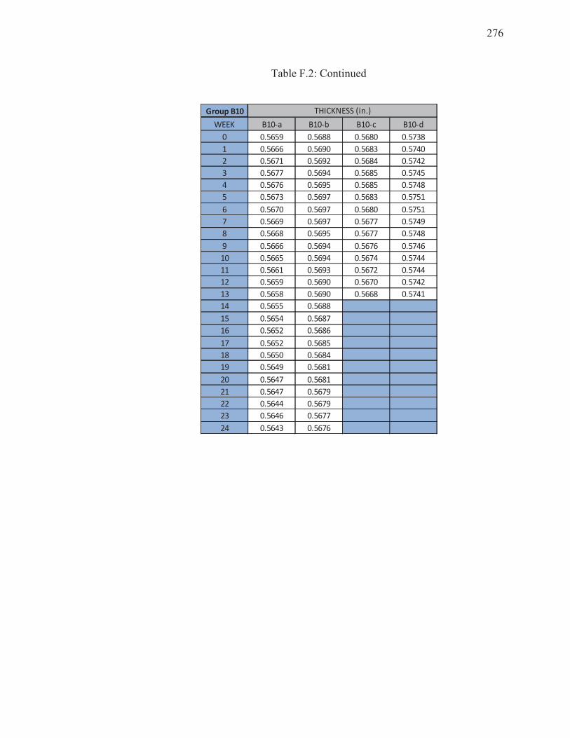
276
Table F.2: Continued
Group B10
WEEK B10-a B10-b B10-c B10-d
0 0.5659 0.5688 0.5680 0.5738
1 0.5666 0.5690 0.5683 0.5740
2 0.5671 0.5692 0.5684 0.5742
3 0.5677 0.5694 0.5685 0.5745
4 0.5676 0.5695 0.5685 0.5748
5 0.5673 0.5697 0.5683 0.5751
6 0.5670 0.5697 0.5680 0.5751
7 0.5669 0.5697 0.5677 0.5749
8 0.5668 0.5695 0.5677 0.5748
9 0.5666 0.5694 0.5676 0.5746
10 0.5665 0.5694 0.5674 0.5744
11 0.5661 0.5693 0.5672 0.5744
12 0.5659 0.5690 0.5670 0.5742
13 0.5658 0.5690 0.5668 0.5741
14 0.5655 0.5688
15 0.5654 0.5687
16 0.5652 0.5686
17 0.5652 0.5685
18 0.5650 0.5684
19 0.5649 0.5681
20 0.5647 0.5681
21 0.5647 0.5679
22 0.5644 0.5679
23 0.5646 0.5677
24 0.5643 0.5676
THICKNESS (in.)
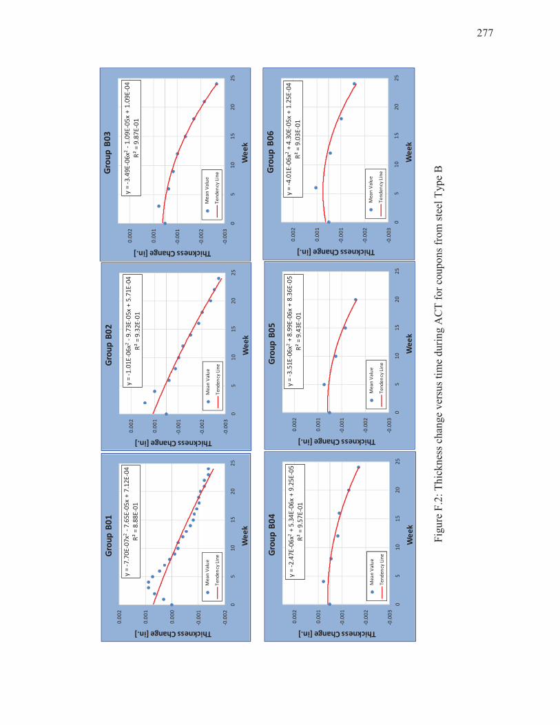
277
Fig
ure
F.2
: T
hic
kn
ess
chan
ge
ver
sus
tim
e d
uri
ng A
CT
fo
r co
up
on
s fr
om
ste
el T
yp
e B
y =
-7
.70
E-0
7x2
-7
.65
E-0
5x
+ 7
.12
E-0
4
R²
= 8
.88
E-0
1
-0.0
02
-0.0
01
0.0
00
0.0
01
0.0
02
05
10
15
20
25
Thickness Change [in.]
We
ek
Gro
up
B0
1
Me
an
Va
lue
Te
nd
en
cy L
ine
y =
-1
.01
E-0
6x2
-9
.73
E-0
5x
+ 5
.71
E-0
4
R²
= 9
.32
E-0
1
-0.0
03
-0.0
02
-0.0
01
0.0
01
0.0
02
05
10
15
20
25
Thickness Change [in.]
We
ek
Gro
up
B0
2
Me
an
Va
lue
Te
nd
en
cy L
ine
y =
-3
.49
E-0
6x2
-1
.09
E-0
5x
+ 1
.09
E-0
4
R²
= 9
.87
E-0
1
-0.0
03
-0.0
02
-0.0
01
0.0
01
0.0
02
05
10
15
20
25
Thickness Change [in.]
We
ek
Gro
up
B0
3
Me
an
Va
lue
Te
nd
en
cy L
ine
y =
-2
.47
E-0
6x2
+ 5
.34
E-0
6x
+ 9
.25
E-0
5
R²
= 9
.57
E-0
1
-0.0
03
-0.0
02
-0.0
01
0.0
01
0.0
02
05
10
15
20
25
Thickness Change [in.]
We
ek
Gro
up
B0
4
Me
an
Va
lue
Te
nd
en
cy L
ine
y =
-3
.51
E-0
6x2
+ 8
.99
E-0
6x
+ 8
.36
E-0
5
R²
= 9
.43
E-0
1
-0.0
03
-0.0
02
-0.0
01
0.0
01
0.0
02
05
10
15
20
25
Thickness Change [in.]
We
ek
Gro
up
B0
5
Me
an
Va
lue
Te
nd
en
cy L
ine
y =
-4
.01
E-0
6x2
+ 4
.30
E-0
5x
+ 1
.25
E-0
4
R²
= 9
.03
E-0
1
-0.0
03
-0.0
02
-0.0
01
0.0
01
0.0
02
05
10
15
20
25
Thickness Change [in.]
We
ek
Gro
up
B0
6
Me
an
Va
lue
Te
nd
en
cy L
ine
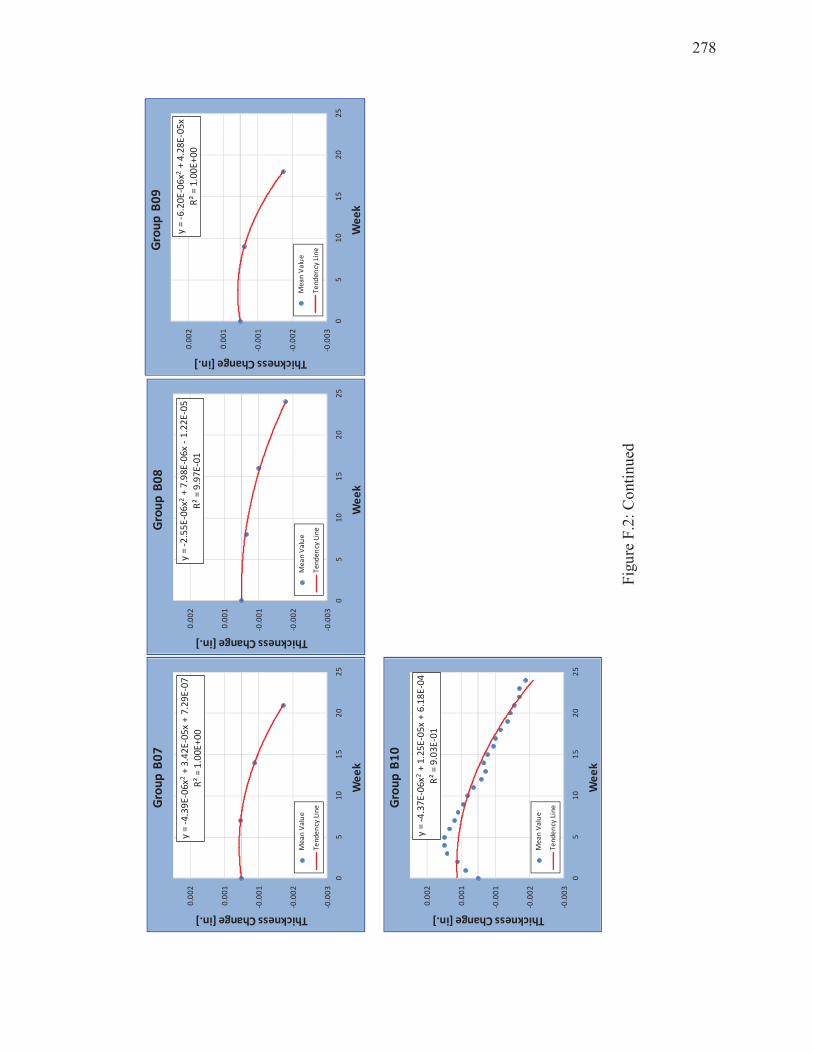
278
Fig
ure
F.2
: C
onti
nu
ed
y =
-4
.39
E-0
6x2
+ 3
.42
E-0
5x
+ 7
.29
E-0
7
R²
= 1
.00
E+
00
-0.0
03
-0.0
02
-0.0
01
0.0
01
0.0
02
05
10
15
20
25
Thickness Change [in.]
We
ek
Gro
up
B0
7
Me
an
Va
lue
Te
nd
en
cy L
ine
y =
-2
.55
E-0
6x2
+ 7
.98
E-0
6x
-1
.22
E-0
5
R²
= 9
.97
E-0
1
-0.0
03
-0.0
02
-0.0
01
0.0
01
0.0
02
05
10
15
20
25
Thickness Change [in.]
We
ek
Gro
up
B0
8
Me
an
Va
lue
Te
nd
en
cy L
ine
y =
-6
.20
E-0
6x2
+ 4
.28
E-0
5x
R²
= 1
.00
E+
00
-0.0
03
-0.0
02
-0.0
01
0.0
01
0.0
02
05
10
15
20
25
Thickness Change [in.]
We
ek
Gro
up
B0
9
Me
an
Va
lue
Te
nd
en
cy L
ine
y =
-4
.37
E-0
6x2
+ 1
.25
E-0
5x
+ 6
.18
E-0
4
R²
= 9
.03
E-0
1
-0.0
03
-0.0
02
-0.0
01
0.0
01
0.0
02
05
10
15
20
25
Thickness Change [in.]
We
ek
Gro
up
B1
0
Me
an
Va
lue
Te
nd
en
cy L
ine
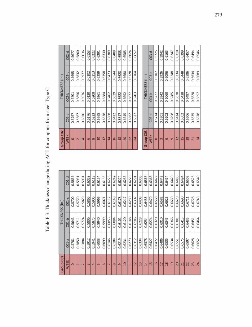
279
Tab
le F
.3:
Thic
kn
ess
chan
ge
du
rin
g A
CT
fo
r co
up
on
s fr
om
ste
el T
yp
e C
Gro
up
C0
1G
rou
p C
02
WE
EK
C0
1-a
C0
1-b
C01
-cC
01
-dW
EE
KC
02
-aC
02
-bC
02
-cC
02-d
00
.57
61
0.5
64
30.
57
00
0.5
85
60
0.5
76
70
.570
10
.56
95
0.5
677
10
.58
50
0.5
71
10.
57
70
0.5
93
12
0.5
86
70
.585
60
.58
32
0.5
860
20
.58
84
0.5
77
40.
58
29
0.5
99
14
0.6
02
00
.597
60
.59
77
0.6
036
30
.59
12
0.5
80
60.
58
66
0.6
06
96
0.6
17
60
.612
00
.61
02
0.6
153
40
.59
41
0.5
87
50.
59
06
0.6
11
88
0.6
22
30
.620
80
.62
13
0.6
222
50
.60
33
0.5
94
00.
59
66
0.6
15
41
00
.62
65
0.6
261
0.6
25
90
.62
91
60
.60
99
0.5
99
90.
60
71
0.6
13
51
20
.63
38
0.6
384
0.6
35
80
.63
30
70
.61
46
0.6
05
30.
61
17
0.6
22
51
40
.63
68
0.6
462
0.6
47
30
.63
89
80
.61
84
0.6
08
40.
61
48
0.6
24
21
60
.64
12
0.6
529
0.6
54
40
.64
88
90
.62
19
0.6
10
10.
61
78
0.6
27
41
80
.65
17
0.6
622
0.6
62
80
.65
38
10
0.6
23
10
.61
20
0.6
21
70
.62
58
20
0.6
54
50
.665
20
.66
80
0.6
58
5
11
0.6
27
90
.61
48
0.6
23
90
.62
70
22
0.6
58
20
.667
70
.67
28
0.6
62
4
12
0.6
31
20
.61
86
0.6
30
70
.62
91
24
0.6
62
70
.670
30
.67
64
0.6
65
7
13
0.6
33
40
.62
28
0.6
40
30
.63
06
14
0.6
37
80
.62
34
0.6
43
30
.63
66
Gro
up
C0
3
15
0.6
42
70
.62
74
0.6
47
90
.63
68
WE
EK
C0
3-a
C0
3-b
C0
3-c
C0
3-d
16
0.6
47
20
.63
20
0.6
56
80
.64
22
00
.57
14
0.5
727
0.5
70
70
.57
25
17
0.6
48
60
.63
10
0.6
58
20
.64
43
30
.59
01
0.5
942
0.5
92
60
.59
42
18
0.6
50
50
.63
43
0.6
62
30
.64
54
60
.62
02
0.6
060
0.6
09
60
.61
63
19
0.6
53
40
.63
66
0.6
65
90
.64
70
90
.62
98
0.6
285
0.6
24
80
.62
47
20
0.6
55
10
.63
81
0.6
67
90
.64
86
12
0.6
41
40
.637
00
.63
34
0.6
31
0
21
0.6
57
50
.64
13
0.6
69
00
.64
94
15
0.6
50
20
.643
80
.64
48
0.6
39
9
22
0.6
59
70
.64
35
0.6
71
10
.65
09
18
0.6
60
60
.649
70
.65
86
0.6
45
7
23
0.6
62
80
.64
51
0.6
72
80
.65
26
21
0.6
63
50
.652
80
.66
34
0.6
49
4
24
0.6
65
20
.64
64
0.6
74
30
.65
40
24
0.6
67
80
.655
70
.66
89
0.6
54
6
TH
ICK
NE
SS
(in
.)
TH
ICK
NE
SS
(in
.)
TH
ICK
NE
SS
(in
.)
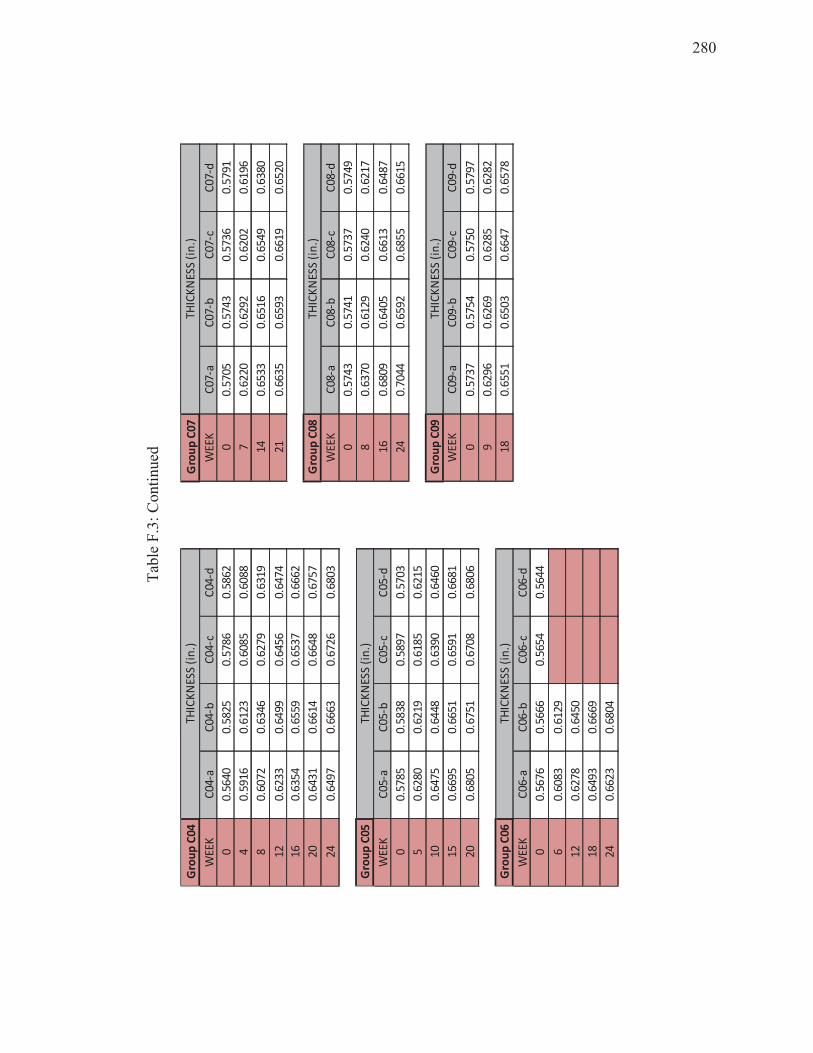
280
Tab
le F
.3:
Co
nti
nu
ed
Gro
up
C04
Gro
up
C07
WEE
KC
04-a
C04
-bC
04-c
C04
-dW
EEK
C07
-aC
07-b
C07
-cC
07-d
00.
5640
0.58
250.
5786
0.58
620
0.57
050.
5743
0.57
360.
5791
40.
5916
0.61
230.
6085
0.60
887
0.62
200.
6292
0.62
020.
6196
80.
6072
0.63
460.
6279
0.63
1914
0.65
330.
6516
0.65
490.
6380
120.
6233
0.64
990.
6456
0.64
7421
0.66
350.
6593
0.66
190.
6520
160.
6354
0.65
590.
6537
0.66
62
200.
6431
0.66
140.
6648
0.67
57G
rou
p C
08
240.
6497
0.66
630.
6726
0.68
03W
EEK
C08
-aC
08-b
C08
-cC
08-d
00.
5743
0.57
410.
5737
0.57
49
Gro
up
C05
80.
6370
0.61
290.
6240
0.62
17
WEE
KC
05-a
C05
-bC
05-c
C05
-d16
0.68
090.
6405
0.66
130.
6487
00.
5785
0.58
380.
5897
0.57
0324
0.70
440.
6592
0.68
550.
6615
50.
6280
0.62
190.
6185
0.62
15
100.
6475
0.64
480.
6390
0.64
60G
rou
p C
09
150.
6695
0.66
510.
6591
0.66
81W
EEK
C09
-aC
09-b
C09
-cC
09-d
200.
6805
0.67
510.
6708
0.68
060
0.57
370.
5754
0.57
500.
5797
90.
6296
0.62
690.
6285
0.62
82
Gro
up
C06
180.
6551
0.65
030.
6647
0.65
78
WEE
KC
06-a
C06
-bC
06-c
C06
-d
00.
5676
0.56
660.
5654
0.56
44
60.
6083
0.61
29
120.
6278
0.64
50
180.
6493
0.66
69
240.
6623
0.68
04
THIC
KN
ESS
(in
.)
THIC
KN
ESS
(in
.)
THIC
KN
ESS
(in
.)
THIC
KN
ESS
(in
.)
THIC
KN
ESS
(in
.)
THIC
KN
ESS
(in
.)

281
Table F.3: Continued
Group C10
WEEK C10-a C10-b C10-c C10-d
0 0.5750 0.5634 0.5784 0.5790
1 0.5833 0.5720 0.5869 0.5899
2 0.5905 0.5807 0.5952 0.5973
3 0.5972 0.5895 0.6011 0.6049
4 0.6041 0.5967 0.6069 0.6096
5 0.6119 0.6028 0.6133 0.6165
6 0.6189 0.6093 0.6217 0.6242
7 0.6263 0.6159 0.6264 0.6349
8 0.6323 0.6238 0.6329 0.6457
9 0.6360 0.6233 0.6339 0.6479
10 0.6419 0.6284 0.6371 0.6479
11 0.6505 0.6315 0.6384 0.6580
12 0.6594 0.6352 0.6459 0.6647
13 0.6654 0.6388 0.6482 0.6748
14 0.6702 0.6406 0.6527 0.6755
15 0.6721 0.6425 0.6555 0.6807
16 0.6780 0.6450 0.6603 0.6881
17 0.6785 0.6481 0.6632 0.6915
18 0.6866 0.6499 0.6684 0.6996
19 0.6896 0.6544 0.6716 0.7034
20 0.6971 0.6557 0.6773 0.7119
21 0.6996 0.6623 0.6792 0.7155
22 0.7017 0.6666 0.6815 0.7184
23 0.7029 0.6692 0.6844 0.7193
24 0.7040 0.6726 0.6871 0.7210
THICKNESS (in.)
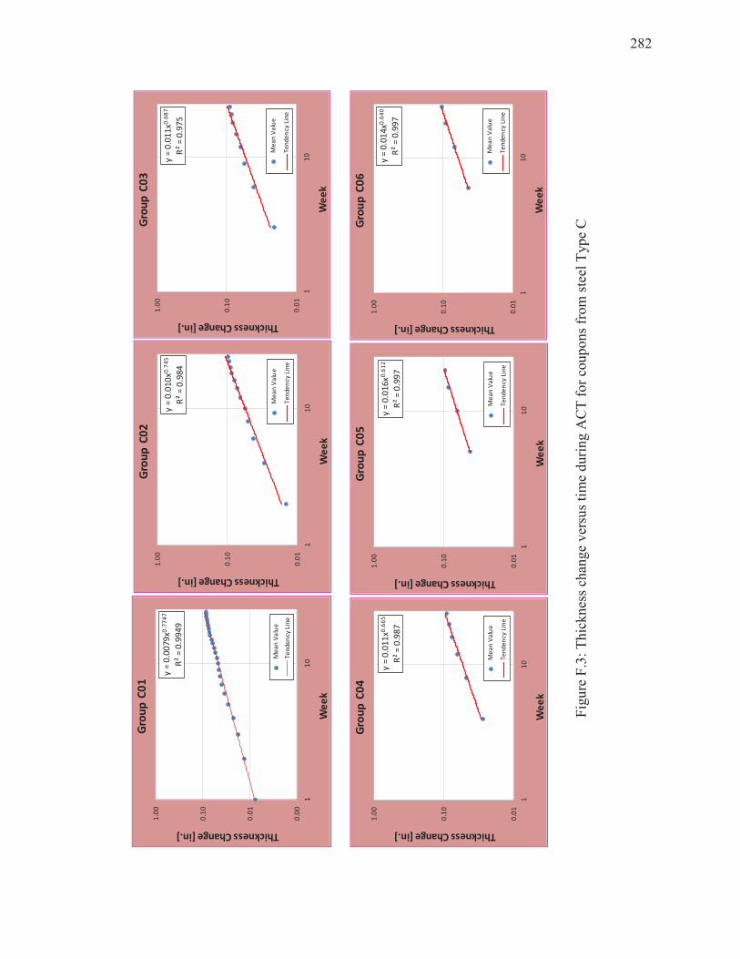
282
Fig
ure
F.3
: T
hic
kn
ess
chan
ge
ver
sus
tim
e d
uri
ng A
CT
fo
r co
up
on
s fr
om
ste
el T
yp
e C
y =
0.0
07
9x0
.77
47
R²
= 0
.99
49
0.0
0
0.0
1
0.1
0
1.0
0
11
0
Thickness Change [in.]
We
ek
Gro
up
C0
1
Me
an
Va
lue
Te
nd
en
cy L
ine
y =
0.0
10
x0.7
45
R²
= 0
.98
4
0.0
1
0.1
0
1.0
0
11
0
Thickness Change [in.]
We
ek
Gro
up
C0
2
Me
an
Va
lue
Te
nd
en
cy L
ine
y =
0.0
11
x0.6
87
R²
= 0
.97
5
0.0
1
0.1
0
1.0
0
11
0
Thickness Change [in.]
We
ek
Gro
up
C0
3
Me
an
Va
lue
Te
nd
en
cy L
ine
y =
0.0
11
x0.6
65
R²
= 0
.98
7
0.0
1
0.1
0
1.0
0
11
0
Thickness Change [in.]
We
ek
Gro
up
C0
4
Me
an
Va
lue
Te
nd
en
cy L
ine
y =
0.0
16
x0.6
12
R²
= 0
.99
7
0.0
1
0.1
0
1.0
0
11
0
Thickness Change [in.]
We
ek
Gro
up
C0
5
Me
an
Va
lue
Te
nd
en
cy L
ine
y =
0.0
14
x0.6
40
R²
= 0
.99
7
0.0
1
0.1
0
1.0
0
11
0
Thickness Change [in.]
We
ek
Gro
up
C0
6
Me
an
Va
lue
Te
nd
en
cy L
ine

283
Fig
ure
F.3
: C
onti
nu
ed
y =
0.0
18
x0.5
25
R²
= 0
.97
3
0.0
1
0.1
0
1.0
0
11
0
Thickness Change [in.]
We
ek
Gro
up
C0
7
Me
an
Va
lue
Te
nd
en
cy L
ine
y =
0.0
12
x0.6
77
R²
= 0
.99
2
0.0
1
0.1
0
1.0
0
11
0
Thickness Change [in.]
We
ek
Gro
up
C0
8
Me
an
Va
lue
Te
nd
en
cy L
ine
y =
0.0
13
x0.6
30
R²
= 1
.00
0
0.0
1
0.1
0
1.0
0
11
0
Thickness Change [in.]
We
ek
Gro
up
C0
9
Me
an
Va
lue
Te
nd
en
cy L
ine
y =
0.0
10
x0.8
12
R²
= 0
.99
6
0.0
0
0.0
1
0.1
0
1.0
0
11
0
Thickness Change [in.]
We
ek
Gro
up
C1
0
Me
an
Va
lue
Te
nd
en
cy L
ine
284
Appendix G Photographs During ACT
The physical aspect changes during the ACT for an uncoated steel coupon is presented
herein. A photography showing the aspect of coupon A01-a was taken every week for the
24 weeks the ACT lasted.
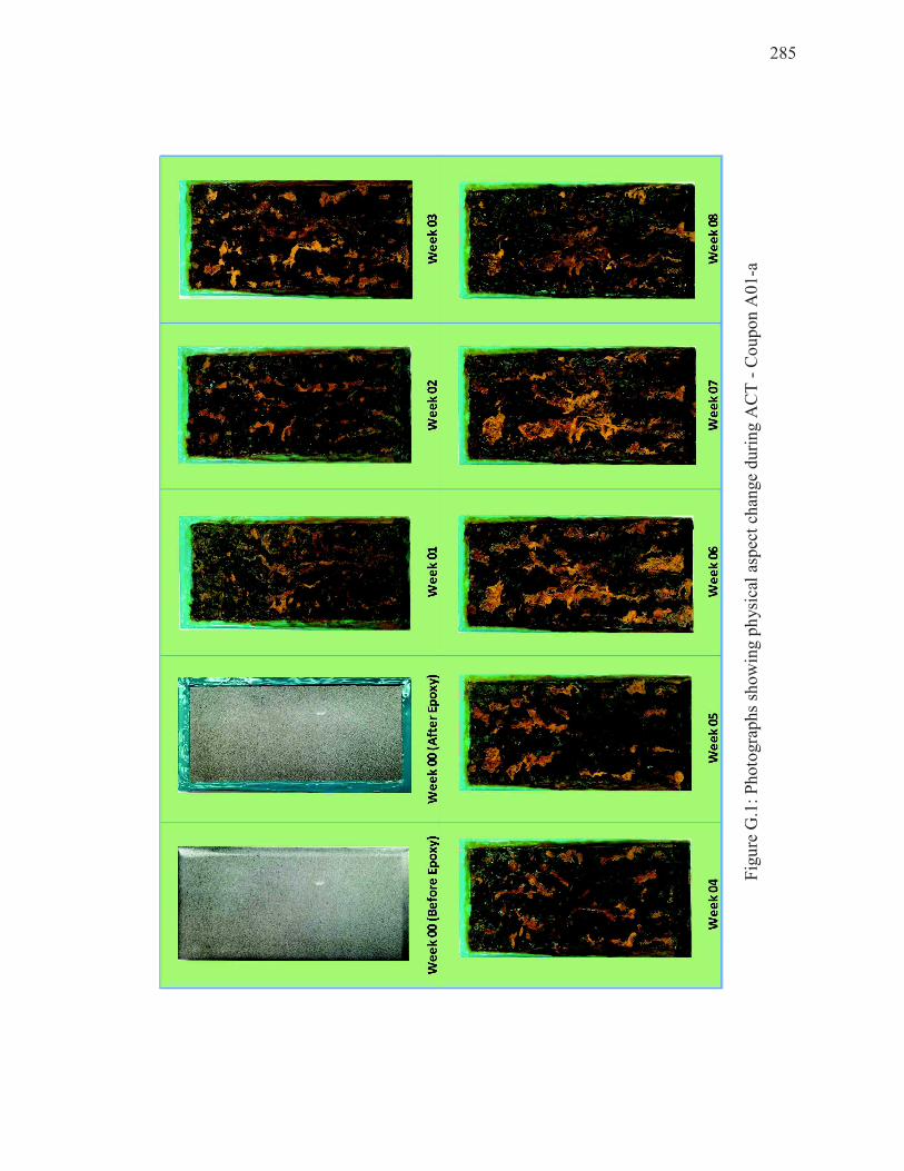
285
Fig
ure
G.1
: P
ho
togra
ph
s sh
ow
ing p
hysi
cal
asp
ect
chan
ge
du
rin
g A
CT
- C
oup
on
A0
1-a
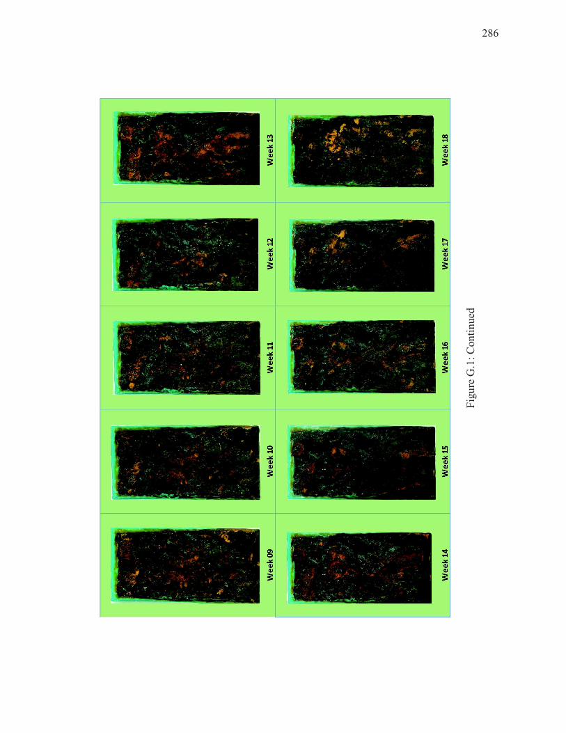
286
Fig
ure
G.1
: C
on
tin
ued
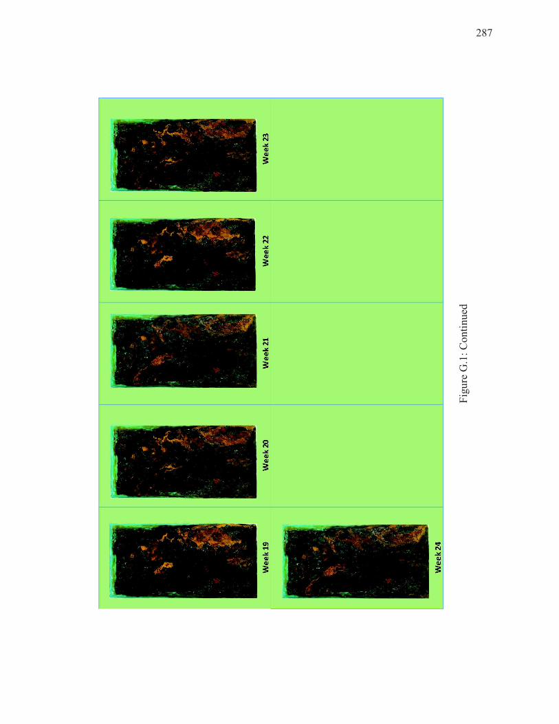
287
Fig
ure
G.1
: C
on
tin
ued

288
Appendix H Creepage Area Change of Scribed Coupons During ACT
Data corresponding to the change of creepage area from steel Type D coupons are
presented herein. Photographs for coupons D01-a and D02-b show the increment of the
NMC from week 0 to week 10. For all coupons from steel Type D are presented the
increment of creepage area in tabulated and graphical manner.
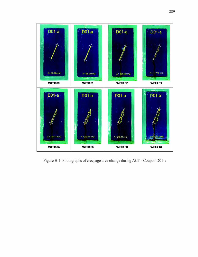
289
Figure H.1: Photographs of creepage area change during ACT - Coupon D01-a
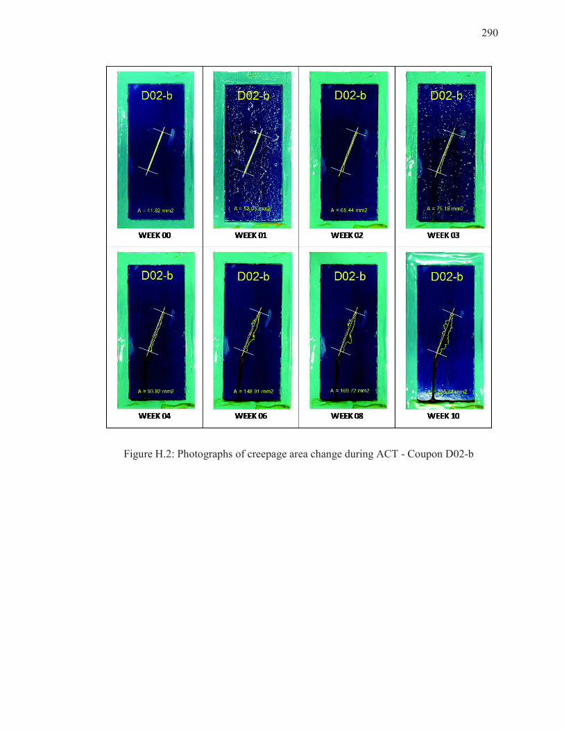
290
Figure H.2: Photographs of creepage area change during ACT - Coupon D02-b
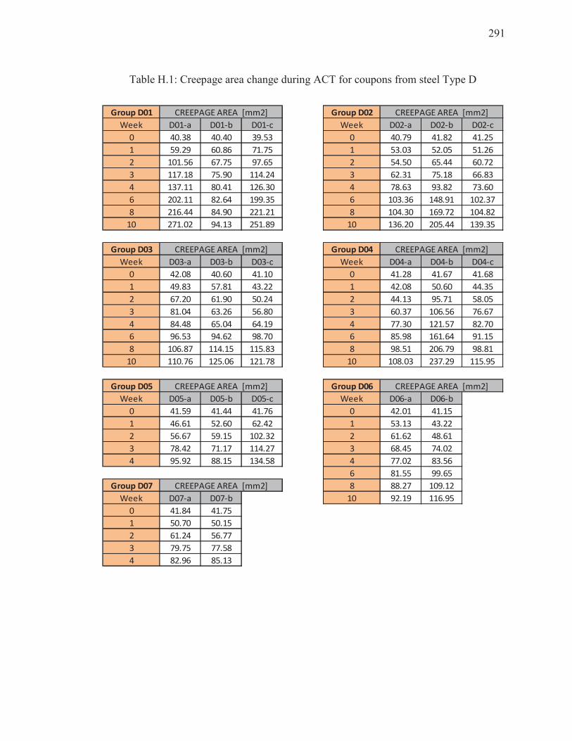
291
Table H.1: Creepage area change during ACT for coupons from steel Type D
Group D01 Group D02
Week D01-a D01-b D01-c Week D02-a D02-b D02-c
0 40.38 40.40 39.53 0 40.79 41.82 41.25
1 59.29 60.86 71.75 1 53.03 52.05 51.26
2 101.56 67.75 97.65 2 54.50 65.44 60.72
3 117.18 75.90 114.24 3 62.31 75.18 66.83
4 137.11 80.41 126.30 4 78.63 93.82 73.60
6 202.11 82.64 199.35 6 103.36 148.91 102.37
8 216.44 84.90 221.21 8 104.30 169.72 104.82
10 271.02 94.13 251.89 10 136.20 205.44 139.35
Group D03 Group D04
Week D03-a D03-b D03-c Week D04-a D04-b D04-c
0 42.08 40.60 41.10 0 41.28 41.67 41.68
1 49.83 57.81 43.22 1 42.08 50.60 44.35
2 67.20 61.90 50.24 2 44.13 95.71 58.05
3 81.04 63.26 56.80 3 60.37 106.56 76.67
4 84.48 65.04 64.19 4 77.30 121.57 82.70
6 96.53 94.62 98.70 6 85.98 161.64 91.15
8 106.87 114.15 115.83 8 98.51 206.79 98.81
10 110.76 125.06 121.78 10 108.03 237.29 115.95
Group D05 Group D06
Week D05-a D05-b D05-c Week D06-a D06-b
0 41.59 41.44 41.76 0 42.01 41.15
1 46.61 52.60 62.42 1 53.13 43.22
2 56.67 59.15 102.32 2 61.62 48.61
3 78.42 71.17 114.27 3 68.45 74.02
4 95.92 88.15 134.58 4 77.02 83.56
6 81.55 99.65
Group D07 8 88.27 109.12
Week D07-a D07-b 10 92.19 116.95
0 41.84 41.75
1 50.70 50.15
2 61.24 56.77
3 79.75 77.58
4 82.96 85.13
CREEPAGE AREA [mm2]
CREEPAGE AREA [mm2]
CREEPAGE AREA [mm2]
CREEPAGE AREA [mm2]
CREEPAGE AREA [mm2] CREEPAGE AREA [mm2]
CREEPAGE AREA [mm2]
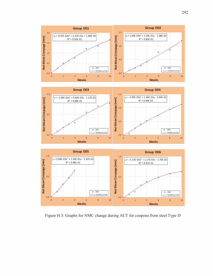
292
Figure H.3: Graphs for NMC change during ACT for coupons from steel Type D
y = -6.05E-03x2 + 2.22E-01x + 1.88E-02
R² = 9.92E-01
0.0
0.5
1.0
1.5
2.0
0 2 4 6 8 10
Ne
t M
ea
n C
ree
pa
ge
[m
m]
Weeks
Group D01
D01
Tendency Line
y = 1.60E-03x2 + 1.03E-01x - 1.08E-02
R² = 9.85E-01
0.0
0.5
1.0
1.5
0 2 4 6 8 10
Ne
t M
ea
n C
ree
pa
ge
[m
m]
Weeks
Group D02
D02
Tendency Line
y = -1.66E-03x2 + 9.84E-02x - 1.12E-02
R² = 9.88E-01
0.0
0.5
1.0
0 2 4 6 8 10
Ne
t M
ea
n C
ree
pa
ge
[m
m]
Weeks
Group D03
D03
Tendency Line
y = -3.05E-03x2 + 1.46E-01x - 3.60E-02
R² = 9.94E-01
0.0
0.5
1.0
1.5
0 2 4 6 8 10
Ne
t M
ea
n C
ree
pa
ge
[m
m]
Weeks
Group D04
D04
Tendency Line
y = 5.98E-03x2 + 1.39E-01x - 5.92E-03
R² = 9.98E-01
0.0
0.5
1.0
0 2 4 6 8 10
Ne
t M
ea
n C
ree
pa
ge
[m
m]
Weeks
Group D05
D05
Tendency Line
y = -5.14E-03x2 + 1.17E-01x - 2.76E-02
R² = 9.87E-01
0.0
0.5
1.0
0 2 4 6 8 10
Ne
t M
ea
n C
ree
pa
ge
[m
m]
Weeks
Group D06
D06
Tendency Line
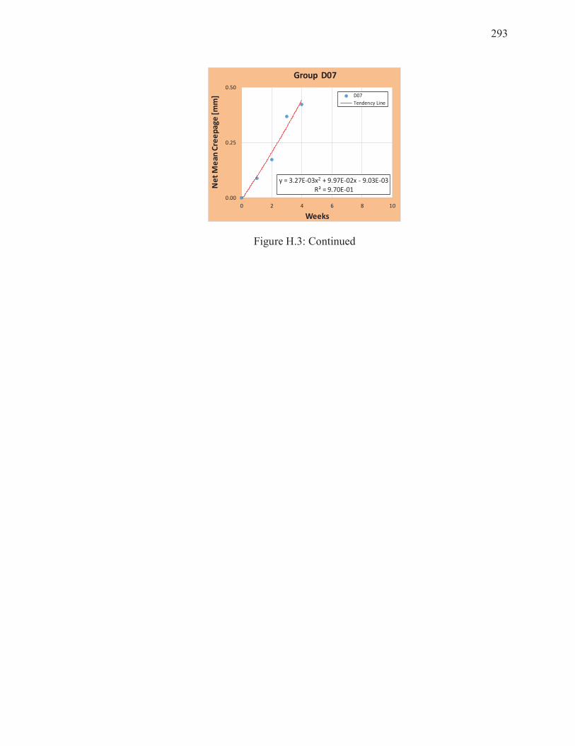
293
Figure H.3: Continued
y = 3.27E-03x2 + 9.97E-02x - 9.03E-03
R² = 9.70E-010.00
0.25
0.50
0 2 4 6 8 10
Ne
t M
ea
n C
ree
pa
ge
[m
m]
Weeks
Group D07
D07
Tendency Line

294
Appendix I Control Test
Data corresponding to the coupons from Control Test are presented in this Appendix. The
codification, and weight change is presented in tables. The physical changes due to the
ACT from the beginning to the end of the test, and the final aspect after sandblasting, are
documented by photographs at those different moments.
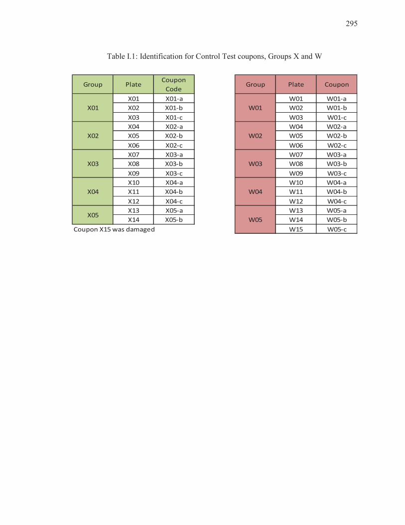
295
Table I.1: Identification for Control Test coupons, Groups X and W
X01 X01-a W01 W01-a
X02 X01-b W02 W01-b
X03 X01-c W03 W01-c
X04 X02-a W04 W02-a
X05 X02-b W05 W02-b
X06 X02-c W06 W02-c
X07 X03-a W07 W03-a
X08 X03-b W08 W03-b
X09 X03-c W09 W03-c
X10 X04-a W10 W04-a
X11 X04-b W11 W04-b
X12 X04-c W12 W04-c
X13 X05-a W13 W05-a
X14 X05-b W14 W05-b
Coupon X15 was damaged W15 W05-c
Coupon
W01
W02
W03
W04
X03
X04
X05
Group Plate
W05
Group PlateCoupon
Code
X01
X02
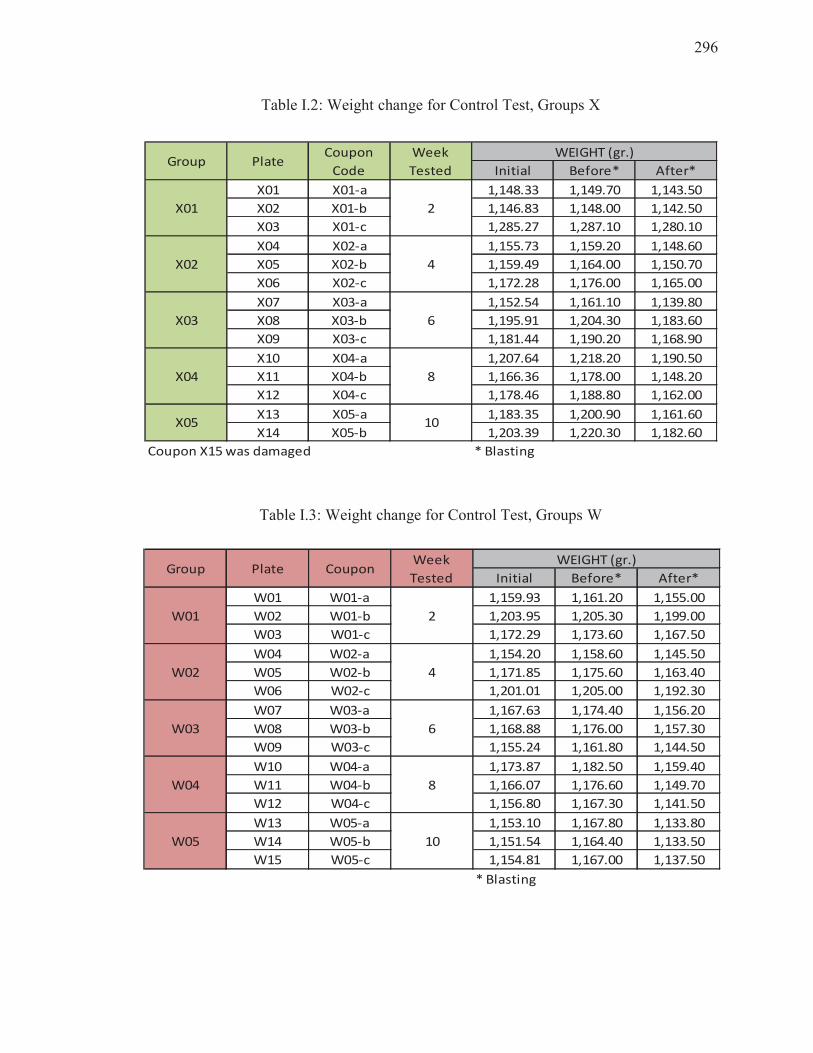
296
Table I.2: Weight change for Control Test, Groups X
Table I.3: Weight change for Control Test, Groups W
Initial Before* After*
X01 X01-a 1,148.33 1,149.70 1,143.50
X02 X01-b 1,146.83 1,148.00 1,142.50
X03 X01-c 1,285.27 1,287.10 1,280.10
X04 X02-a 1,155.73 1,159.20 1,148.60
X05 X02-b 1,159.49 1,164.00 1,150.70
X06 X02-c 1,172.28 1,176.00 1,165.00
X07 X03-a 1,152.54 1,161.10 1,139.80
X08 X03-b 1,195.91 1,204.30 1,183.60
X09 X03-c 1,181.44 1,190.20 1,168.90
X10 X04-a 1,207.64 1,218.20 1,190.50
X11 X04-b 1,166.36 1,178.00 1,148.20
X12 X04-c 1,178.46 1,188.80 1,162.00
X13 X05-a 1,183.35 1,200.90 1,161.60
X14 X05-b 1,203.39 1,220.30 1,182.60
Coupon X15 was damaged * Blasting
2
4
6
8
10
WEIGHT (gr.)Group Plate
Coupon
Code
Week
Tested
X01
X04
X05
X02
X03
Initial Before* After*
W01 W01-a 1,159.93 1,161.20 1,155.00
W02 W01-b 1,203.95 1,205.30 1,199.00
W03 W01-c 1,172.29 1,173.60 1,167.50
W04 W02-a 1,154.20 1,158.60 1,145.50
W05 W02-b 1,171.85 1,175.60 1,163.40
W06 W02-c 1,201.01 1,205.00 1,192.30
W07 W03-a 1,167.63 1,174.40 1,156.20
W08 W03-b 1,168.88 1,176.00 1,157.30
W09 W03-c 1,155.24 1,161.80 1,144.50
W10 W04-a 1,173.87 1,182.50 1,159.40
W11 W04-b 1,166.07 1,176.60 1,149.70
W12 W04-c 1,156.80 1,167.30 1,141.50
W13 W05-a 1,153.10 1,167.80 1,133.80
W14 W05-b 1,151.54 1,164.40 1,133.50
W15 W05-c 1,154.81 1,167.00 1,137.50
* Blasting
Group Plate CouponWeek
Tested
WEIGHT (gr.)
W01 2
W02 4
W03 6
W04 8
W05 10
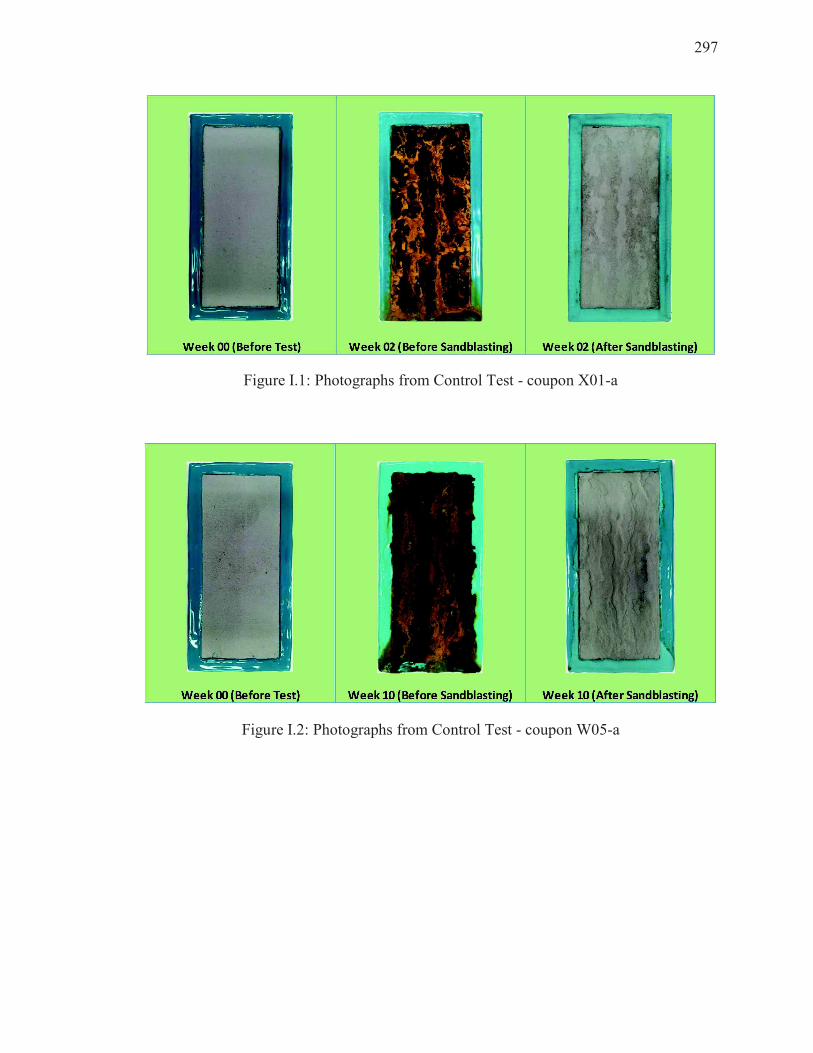
297
Figure I.1: Photographs from Control Test - coupon X01-a
Figure I.2: Photographs from Control Test - coupon W05-a
298
Appendix J Rating Factors RFm and RFv
The load rating factors for bending capacity RFm and shear capacity RFv, corresponding
to the 96 bridge cases considered in the parametric study for this research are presented
from Figures J.1 to J.24. Both RFm and RFv values were calculated and plotted at ages 0,
20, 40, 60, 80, and 100 years of bridge service life. The factors RFm and RFv were
evaluated for the load levels: Inventory, Operating, and Legal. For each rating plot the
limit factor 1.0 is marked with a red line to emphasize the trigger age when some actions
must be taken, according to the prescriptions given by the AASHTO MBE (AASHTO,
2011).
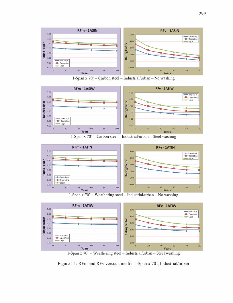
299
1-Span x 70’ – Carbon steel – Industrial/urban – No washing
1-Span x 70’ – Carbon steel – Industrial/urban – Steel washing
1-Span x 70’ – Weathering steel – Industrial/urban – No washing
1-Span x 70’ – Weathering steel – Industrial/urban – Steel washing
Figure J.1: RFm and RFv versus time for 1-Span x 70’, Industrial/urban
0.00
0.50
1.00
1.50
2.00
2.50
3.00
3.50
0 20 40 60 80 100
Ra
tin
g F
act
or
Years
RFm - 1ASIN
Inventory
Operating
Legal0.00
1.00
2.00
3.00
4.00
5.00
0 20 40 60 80 100
Ra
tin
g Fa
cto
r
Years
RFv - 1ASIN
Inventory
Operating
Legal
0.00
0.50
1.00
1.50
2.00
2.50
3.00
3.50
0 20 40 60 80 100
Ra
tin
g F
act
or
Years
RFm - 1ASIW
Inventory
Operating
Legal0.00
1.00
2.00
3.00
4.00
5.00
0 20 40 60 80 100R
ati
ng
Fa
cto
r
Years
RFv - 1ASIW
Inventory
Operating
Legal
0.00
0.50
1.00
1.50
2.00
2.50
3.00
3.50
0 20 40 60 80 100
Ra
tin
g F
act
or
Years
RFm - 1ATIN
Inventory
Operating
Legal0.00
1.00
2.00
3.00
4.00
5.00
0 20 40 60 80 100
Ra
tin
g F
act
or
Years
RFv - 1ATIN
Inventory
Operating
Legal
0.00
0.50
1.00
1.50
2.00
2.50
3.00
3.50
0 20 40 60 80 100
Ra
ctin
g F
act
or
Years
RFm - 1ATIW
Inventory
Operating
Legal0.00
1.00
2.00
3.00
4.00
5.00
0 20 40 60 80 100
Ra
tin
g F
act
or
Years
RFv - 1ATIW
Inventory
Operating
Legal
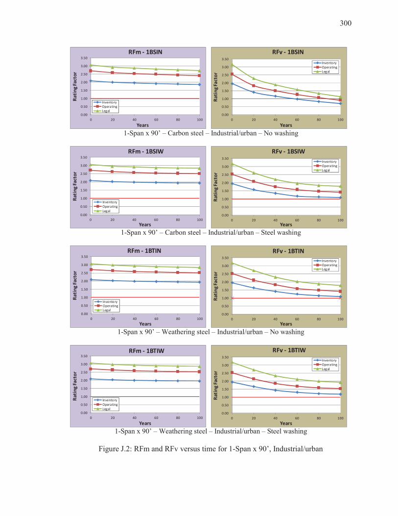
300
1-Span x 90’ – Carbon steel – Industrial/urban – No washing
1-Span x 90’ – Carbon steel – Industrial/urban – Steel washing
1-Span x 90’ – Weathering steel – Industrial/urban – No washing
1-Span x 90’ – Weathering steel – Industrial/urban – Steel washing
Figure J.2: RFm and RFv versus time for 1-Span x 90’, Industrial/urban
0.00
0.50
1.00
1.50
2.00
2.50
3.00
3.50
0 20 40 60 80 100
Ra
tin
g F
act
or
Years
RFm - 1BSIN
Inventory
Operating
Legal0.00
0.50
1.00
1.50
2.00
2.50
3.00
3.50
0 20 40 60 80 100
Ra
tin
g F
act
or
Years
RFv - 1BSIN
Inventory
Operating
Legal
0.00
0.50
1.00
1.50
2.00
2.50
3.00
3.50
0 20 40 60 80 100
Ra
tin
g F
act
or
Years
RFm - 1BSIW
Inventory
Operating
Legal0.00
0.50
1.00
1.50
2.00
2.50
3.00
3.50
0 20 40 60 80 100R
ati
ng
Fa
cto
r
Years
RFv - 1BSIW
Inventory
Operating
Legal
0.00
0.50
1.00
1.50
2.00
2.50
3.00
3.50
0 20 40 60 80 100
Ra
tin
g F
act
or
Years
RFm - 1BTIN
InventoryOperatingLegal
0.00
0.50
1.00
1.50
2.00
2.50
3.00
3.50
0 20 40 60 80 100
Ra
tin
g F
act
or
Years
RFv - 1BTIN
InventoryOperatingLegal
0.00
0.50
1.00
1.50
2.00
2.50
3.00
3.50
0 20 40 60 80 100
Ra
tin
g F
act
or
Years
RFm - 1BTIW
Inventory
Operating
Legal
0.00
0.50
1.00
1.50
2.00
2.50
3.00
3.50
0 20 40 60 80 100
Ra
tin
g F
act
or
Years
RFv - 1BTIW
Inventory
Operating
Legal
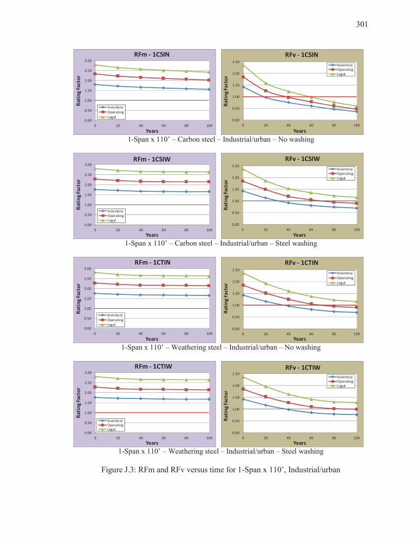
301
1-Span x 110’ – Carbon steel – Industrial/urban – No washing
1-Span x 110’ – Carbon steel – Industrial/urban – Steel washing
1-Span x 110’ – Weathering steel – Industrial/urban – No washing
1-Span x 110’ – Weathering steel – Industrial/urban – Steel washing
Figure J.3: RFm and RFv versus time for 1-Span x 110’, Industrial/urban
0.00
0.50
1.00
1.50
2.00
2.50
3.00
0 20 40 60 80 100
Ra
tin
g F
act
or
Years
RFm - 1CSIN
Inventory
Operating
Legal0.00
0.50
1.00
1.50
2.00
2.50
0 20 40 60 80 100
Ra
tin
g F
act
or
Years
RFv - 1CSIN
Inventory
Operating
Legal
0.00
0.50
1.00
1.50
2.00
2.50
3.00
0 20 40 60 80 100
Ra
tin
g F
act
or
Years
RFm - 1CSIW
Inventory
Operating
Legal0.00
0.50
1.00
1.50
2.00
2.50
0 20 40 60 80 100R
ati
ng
Fa
cto
r
Years
RFv - 1CSIW
Inventory
Operating
Legal
0.00
0.50
1.00
1.50
2.00
2.50
3.00
0 20 40 60 80 100
Ra
tin
g F
act
or
Years
RFm - 1CTIN
Inventory
Operating
Legal0.00
0.50
1.00
1.50
2.00
2.50
0 20 40 60 80 100
Ra
tin
g F
act
or
Years
RFv - 1CTIN
Inventory
Operating
Legal
0.00
0.50
1.00
1.50
2.00
2.50
3.00
0 20 40 60 80 100
Ra
tin
g F
act
or
Years
RFm - 1CTIW
InventoryOperatingLegal
0.00
0.50
1.00
1.50
2.00
2.50
0 20 40 60 80 100
Ra
tin
g F
act
or
Years
RFv - 1CTIW
InventoryOperatingLegal

302
1-Span x 130’ – Carbon steel – Industrial/urban – No washing
1-Span x 130’ – Carbon steel – Industrial/urban – Steel washing
1-Span x 130’ – Weathering steel – Industrial/urban – No washing
1-Span x 130’ – Weathering steel – Industrial/urban – Steel washing
Figure J.4: RFm and RFv versus time for 1-Span x 130’, Industrial/urban
0.00
0.50
1.00
1.50
2.00
2.50
3.00
3.50
0 20 40 60 80 100
Ra
tin
g F
act
or
Years
RFm - 1DSIN
Inventory
Operating
Legal0.00
0.50
1.00
1.50
2.00
2.50
3.00
0 20 40 60 80 100
Ra
tin
g F
act
or
Years
RFv - 1DSIN
InventoryOperatingLegal
0.00
0.50
1.00
1.50
2.00
2.50
3.00
3.50
0 20 40 60 80 100
Ra
tin
g F
act
or
Years
RFm - 1DSIW
InventoryOperatingLegal
0.00
0.50
1.00
1.50
2.00
2.50
3.00
0 20 40 60 80 100R
ati
ng
Fa
cto
r
Years
RFv - 1DSIW
InventoryOperatingLegal
0.00
0.50
1.00
1.50
2.00
2.50
3.00
3.50
0 20 40 60 80 100
Ra
tin
g F
act
or
Years
RFm - 1DTIN
InventoryOperatingLegal
0.00
0.50
1.00
1.50
2.00
2.50
3.00
0 20 40 60 80 100
Ra
tin
g F
act
or
Years
RFv - 1DTIN
Inventory
Operating
Legal
0.00
0.50
1.00
1.50
2.00
2.50
3.00
3.50
0 20 40 60 80 100
Ra
tin
g F
act
or
Years
RFm - 1DTIW
InventoryOperatingLegal
0.00
0.50
1.00
1.50
2.00
2.50
3.00
0 20 40 60 80 100
Ra
tin
g F
act
or
Years
RFv - 1DTIW
Inventory
Operating
Legal
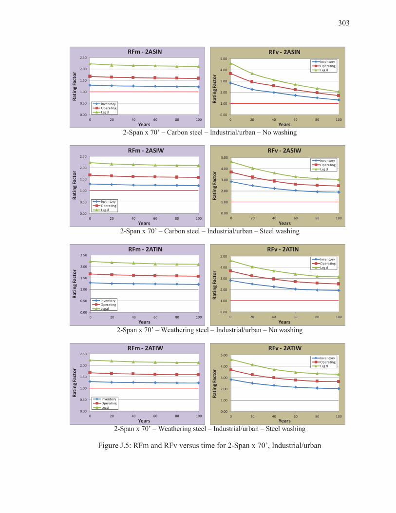
303
2-Span x 70’ – Carbon steel – Industrial/urban – No washing
2-Span x 70’ – Carbon steel – Industrial/urban – Steel washing
2-Span x 70’ – Weathering steel – Industrial/urban – No washing
2-Span x 70’ – Weathering steel – Industrial/urban – Steel washing
Figure J.5: RFm and RFv versus time for 2-Span x 70’, Industrial/urban
0.00
0.50
1.00
1.50
2.00
2.50
0 20 40 60 80 100
Ra
tin
g F
act
or
Years
RFm - 2ASIN
InventoryOperatingLegal
0.00
1.00
2.00
3.00
4.00
5.00
0 20 40 60 80 100
Ra
tin
g F
act
or
Years
RFv - 2ASIN
InventoryOperatingLegal
0.00
0.50
1.00
1.50
2.00
2.50
0 20 40 60 80 100
Ra
tin
g F
act
or
Years
RFm - 2ASIW
InventoryOperatingLegal
0.00
1.00
2.00
3.00
4.00
5.00
0 20 40 60 80 100R
ati
ng
Fa
cto
r
Years
RFv - 2ASIW
Inventory
Operating
Legal
0.00
0.50
1.00
1.50
2.00
2.50
0 20 40 60 80 100
Ra
tin
g F
act
or
Years
RFm - 2ATIN
InventoryOperatingLegal
0.00
1.00
2.00
3.00
4.00
5.00
0 20 40 60 80 100
Ra
tin
g F
act
or
Years
RFv - 2ATIN
InventoryOperatingLegal
0.00
0.50
1.00
1.50
2.00
2.50
0 20 40 60 80 100
Ra
tin
g F
act
or
Years
RFm - 2ATIW
InventoryOperatingLegal
0.00
1.00
2.00
3.00
4.00
5.00
0 20 40 60 80 100
Ra
tin
g F
act
or
Years
RFv - 2ATIW
InventoryOperatingLegal

304
2-Span x 90’ – Carbon steel – Industrial/urban – No washing
2-Span x 90’ – Carbon steel – Industrial/urban – Steel washing
2-Span x 90’ – Weathering steel – Industrial/urban – No washing
2-Span x 90’ – Weathering steel – Industrial/urban – Steel washing
Figure J.6: RFm and RFv versus time for 2-Span x 90’, Industrial/urban
0.00
0.50
1.00
1.50
2.00
2.50
0 20 40 60 80 100
Ra
tin
g F
act
or
Years
RFm - 2BSIN
Inventory
Operating
Legal0.00
1.00
2.00
3.00
4.00
0 20 40 60 80 100
Ra
tin
g F
act
or
Years
RFv - 2BSIN
InventoryOperatingLegal
0.00
0.50
1.00
1.50
2.00
2.50
0 20 40 60 80 100
Ra
tin
g F
act
or
Years
RFm - 2BSIW
Inventory
Operating
Legal0.00
1.00
2.00
3.00
4.00
0 20 40 60 80 100R
ati
ng
Fa
cto
r
Years
RFv - 2BSIW
InventoryOperatingLegal
0.00
0.50
1.00
1.50
2.00
2.50
0 20 40 60 80 100
Ra
tin
g F
act
or
Years
RFm - 2BTIN
InventoryOperatingLegal
0.00
1.00
2.00
3.00
4.00
0 20 40 60 80 100
Ra
tin
g F
act
or
Years
RFv - 2BTIN
InventoryOperatingLegal
0.00
0.50
1.00
1.50
2.00
2.50
0 20 40 60 80 100
Ra
tin
g F
act
or
Years
RFm - 2BTIW
InventoryOperatingLegal
0.00
1.00
2.00
3.00
4.00
0 20 40 60 80 100
Ra
tin
g F
act
or
Years
RFv - 2BTIW
InventoryOperatingLegal

305
2-Span x 110’ – Carbon steel – Industrial/urban – No washing
2-Span x 110’ – Carbon steel – Industrial/urban – Steel washing
2-Span x 110’ – Weathering steel – Industrial/urban – No washing
2-Span x 110’ – Weathering steel – Industrial/urban – Steel washing
Figure J.7: RFm and RFv versus time for 2-Span x 110’, Industrial/urban
0.00
0.50
1.00
1.50
2.00
2.50
0 20 40 60 80 100
Ra
tin
g F
act
or
Years
RFm - 2CSIN
InventoryOperatingLegal
0.00
0.50
1.00
1.50
2.00
2.50
3.00
0 20 40 60 80 100
Ra
tin
g F
act
or
Years
RFv - 2CSIN
Inventory
Operating
Legal
0.00
0.50
1.00
1.50
2.00
2.50
0 20 40 60 80 100
Ra
tin
g F
act
or
Years
RFm - 2CSIW
Inventory
Operating
Legal0.00
0.50
1.00
1.50
2.00
2.50
3.00
0 20 40 60 80 100R
ati
ng
Fa
cto
r
Years
RFv - 2CSIW
Inventory
Operating
Legal
0.00
0.50
1.00
1.50
2.00
2.50
0 20 40 60 80 100
Ra
tin
g F
act
or
Years
RFm - 2CTIN
Inventory
Operating
Legal0.00
0.50
1.00
1.50
2.00
2.50
3.00
0 20 40 60 80 100
Ra
tin
g F
act
or
Years
RFv - 2CTIN
Inventory
Operating
Legal
0.00
0.50
1.00
1.50
2.00
2.50
0 20 40 60 80 100
Ra
tin
g F
act
or
Years
RFm - 2CTIW
InventoryOperatingLegal
0.00
0.50
1.00
1.50
2.00
2.50
3.00
0 20 40 60 80 100
Ra
tin
g F
act
or
Years
RFv - 2CTIW
Inventory
Operating
Legal

306
2-Span x 130’ – Carbon steel – Industrial/urban – No washing
2-Span x 130’ – Carbon steel – Industrial/urban – Steel washing
2-Span x 130’ – Weathering steel – Industrial/urban – No washing
2-Span x 130’ – Weathering steel – Industrial/urban – Steel washing
Figure J.8: RFm and RFv versus time for 2-Span x 130’, Industrial/urban
0.00
0.50
1.00
1.50
2.00
0 20 40 60 80 100
Ra
tin
g F
act
or
Years
RFm - 2DSIN
Inventory
Operating
Legal0.00
1.00
2.00
3.00
4.00
0 20 40 60 80 100
Ra
tin
g F
act
or
Years
RFv - 2DSIN
InventoryOperatingLegal
0.00
0.50
1.00
1.50
2.00
0 20 40 60 80 100
Ra
tin
g f
act
or
Years
RFm - 2DSIW
InventoryOperatingLegal
0.00
1.00
2.00
3.00
4.00
0 20 40 60 80 100R
ati
ng
Fa
cto
r
Years
RFv - 2DSIW
Inventory
Operating
Legal
0.00
0.50
1.00
1.50
2.00
0 20 40 60 80 100
Ra
tin
g F
act
or
Years
RFm - 2DTIN
InventoryOperatingLegal
0.00
1.00
2.00
3.00
4.00
0 20 40 60 80 100
Ra
tin
g F
act
or
Years
RFv - 2DTIN
InventoryOperatingLegal
0.00
0.50
1.00
1.50
2.00
0 20 40 60 80 100
Ra
tin
g F
act
or
Years
RFm - 2DTIW
InventoryOperatingLegal
0.00
1.00
2.00
3.00
0 20 40 60 80 100
Ra
tin
g F
act
or
Years
RFv - 2DTIW
InventoryOperatingLegal
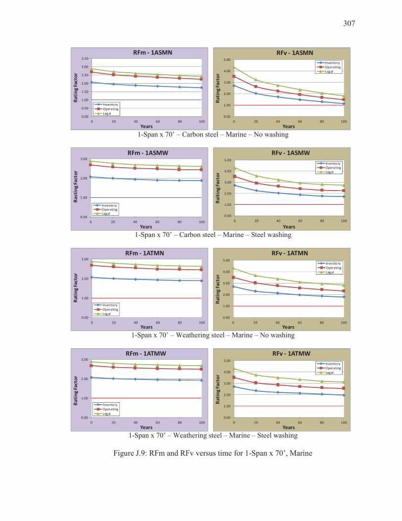
307
1-Span x 70’ – Carbon steel – Marine – No washing
1-Span x 70’ – Carbon steel – Marine – Steel washing
1-Span x 70’ – Weathering steel – Marine – No washing
1-Span x 70’ – Weathering steel – Marine – Steel washing
Figure J.9: RFm and RFv versus time for 1-Span x 70’, Marine
0.00
0.50
1.00
1.50
2.00
2.50
3.00
3.50
0 20 40 60 80 100
Ra
tin
g F
act
or
Years
RFm - 1ASMN
Inventory
Operating
Legal0.00
1.00
2.00
3.00
4.00
5.00
0 20 40 60 80 100
Ra
tin
g F
act
or
Years
RFv - 1ASMN
Inventory
Operating
Legal
0.00
1.00
2.00
3.00
0 20 40 60 80 100
Ra
stin
g F
act
or
Years
RFm - 1ASMW
InventoryOperatingLegal
0.00
1.00
2.00
3.00
4.00
5.00
0 20 40 60 80 100R
ait
ing
Fa
cto
r
Years
RFv - 1ASMW
InventoryOperatingLegal
0.00
1.00
2.00
3.00
0 20 40 60 80 100
Ra
tin
g F
act
or
Years
RFm - 1ATMN
Inventory
Operating
Legal0.00
1.00
2.00
3.00
4.00
5.00
0 20 40 60 80 100
Ra
tin
g F
act
or
Years
RFv - 1ATMN
Inventory
Operating
Legal
0.00
1.00
2.00
3.00
0 20 40 60 80 100
Ra
tin
g F
act
or
Years
RFm - 1ATMW
Inventory
Operating
Legal0.00
1.00
2.00
3.00
4.00
5.00
0 20 40 60 80 100
Ra
tin
g F
act
or
Years
RFv - 1ATMW
Inventory
Operating
Legal
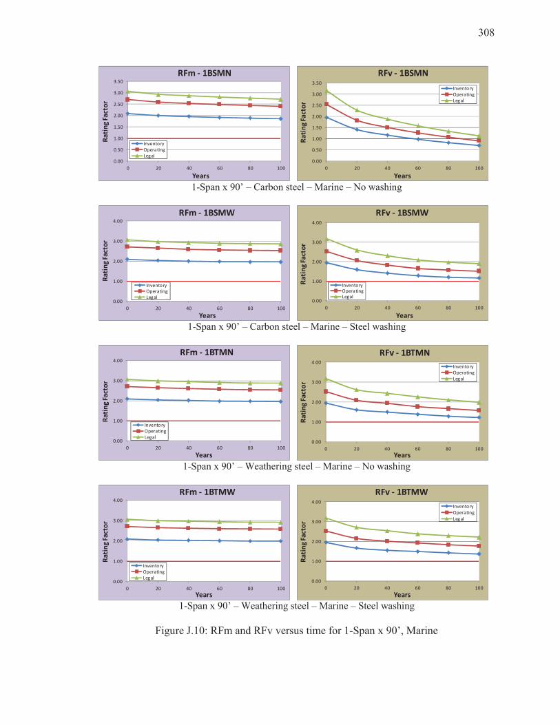
308
1-Span x 90’ – Carbon steel – Marine – No washing
1-Span x 90’ – Carbon steel – Marine – Steel washing
1-Span x 90’ – Weathering steel – Marine – No washing
1-Span x 90’ – Weathering steel – Marine – Steel washing
Figure J.10: RFm and RFv versus time for 1-Span x 90’, Marine
0.00
0.50
1.00
1.50
2.00
2.50
3.00
3.50
0 20 40 60 80 100
Ra
tin
g F
act
or
Years
RFm - 1BSMN
Inventory
Operating
Legal0.00
0.50
1.00
1.50
2.00
2.50
3.00
3.50
0 20 40 60 80 100
Ra
tin
g F
act
or
Years
RFv - 1BSMN
Inventory
Operating
Legal
0.00
1.00
2.00
3.00
4.00
0 20 40 60 80 100
Ra
tin
g F
act
or
Years
RFm - 1BSMW
InventoryOperatingLegal
0.00
1.00
2.00
3.00
4.00
0 20 40 60 80 100R
ati
ng
Fa
cto
r
Years
RFv - 1BSMW
InventoryOperatingLegal
0.00
1.00
2.00
3.00
4.00
0 20 40 60 80 100
Ra
tin
g F
act
or
Years
RFm - 1BTMN
Inventory
Operating
Legal0.00
1.00
2.00
3.00
4.00
0 20 40 60 80 100
Ra
tin
g F
act
or
Years
RFv - 1BTMN
Inventory
Operating
Legal
0.00
1.00
2.00
3.00
4.00
0 20 40 60 80 100
Ra
tin
g F
act
or
Years
RFm - 1BTMW
Inventory
Operating
Legal0.00
1.00
2.00
3.00
4.00
0 20 40 60 80 100
Ra
tin
g F
act
or
Years
RFv - 1BTMW
Inventory
Operating
Legal

309
1-Span x 110’ – Carbon steel – Marine – No washing
1-Span x 110’ – Carbon steel – Marine – Steel washing
1-Span x 110’ – Weathering steel – Marine – No washing
1-Span x 110’ – Weathering steel – Marine – Steel washing
Figure J.11: RFm and RFv versus time for 1-Span x 110’, Marine
0.00
0.50
1.00
1.50
2.00
2.50
3.00
0 20 40 60 80 100
Ra
tin
g F
act
or
Years
RFm - 1CSMN
Inventory
Operating
Legal0.00
0.50
1.00
1.50
2.00
2.50
0 20 40 60 80 100
Ra
tin
g F
act
or
Years
RFv - 1CSMN
Inventory
Operating
Legal
0.00
0.50
1.00
1.50
2.00
2.50
3.00
0 20 40 60 80 100
Ra
tin
g F
act
or
Years
RFm - 1CSMW
InventoryOperatingLegal
0.00
0.50
1.00
1.50
2.00
2.50
0 20 40 60 80 100R
ati
ng
Fa
cto
r
Years
RFv - 1CSMW
InventoryOperatingLegal
0.00
0.50
1.00
1.50
2.00
2.50
3.00
0 20 40 60 80 100
Ra
tin
g F
act
or
Years
RFm - 1CTMN
InventoryOperatingLegal
0.00
0.50
1.00
1.50
2.00
2.50
0 20 40 60 80 100
Ra
tin
g F
act
or
Years
RFv - 1CTMN
InventoryOperatingLegal
0.00
0.50
1.00
1.50
2.00
2.50
3.00
0 20 40 60 80 100
Ra
tin
g F
act
or
Years
RFm - 1CTMW
InventoryOperatingLegal
0.00
0.50
1.00
1.50
2.00
2.50
0 20 40 60 80 100
Ra
tin
g F
act
or
Years
RFv - 1CTMW
InventoryOperatingLegal

310
1-Span x 130’ – Carbon steel – Marine – No washing
1-Span x 130’ – Carbon steel – Marine – Steel washing
1-Span x 130’ – Weathering steel – Marine – No washing
1-Span x 130’ – Weathering steel – Marine – Steel washing
Figure J.12: RFm and RFv versus time for 1-Span x 130’, Marine
0.00
0.50
1.00
1.50
2.00
2.50
3.00
3.50
0 20 40 60 80 100
Ra
tin
g F
act
or
Years
RFm - 1DSMN
Inventory
Operating
Legal0.00
0.50
1.00
1.50
2.00
2.50
3.00
0 20 40 60 80 100
Ra
tin
g F
act
or
Years
RFv - 1DSMN
InventoryOperatingLegal
0.00
1.00
2.00
3.00
4.00
0 20 40 60 80 100
Ra
tin
g F
act
or
Years
RFm - 1DSMW
Inventory
Operating
Legal0.00
0.50
1.00
1.50
2.00
2.50
3.00
0 20 40 60 80 100R
ati
ng
Fa
cto
r
Years
RFv - 1DSMW
Inventory
Operating
Legal
0.00
1.00
2.00
3.00
4.00
0 20 40 60 80 100
Ra
tin
g F
act
or
Years
RFm - 1DTMN
Inventory
Operating
Legal0.00
0.50
1.00
1.50
2.00
2.50
3.00
0 20 40 60 80 100
Ra
tin
g F
act
or
Years
RFv - 1DTMN
InventoryOperatingLegal
0.00
1.00
2.00
3.00
4.00
0 20 40 60 80 100
Ra
tin
g F
act
or
Years
RFm - 1DTMW
InventoryOperatingLegal
0.00
0.50
1.00
1.50
2.00
2.50
3.00
0 20 40 60 80 100
Ra
tin
g F
act
or
Years
RFv - 1DTMW
Inventory
Operating
Legal

311
2-Span x 70’ – Carbon steel – Marine – No washing
2-Span x 70’ – Carbon steel – Marine – Steel washing
2-Span x 70’ – Weathering steel – Marine – No washing
2-Span x 70’ – Weathering steel – Marine – Steel washing
Figure J.13: RFm and RFv versus time for 2-Span x 70’, Marine
0.00
0.50
1.00
1.50
2.00
2.50
0 20 40 60 80 100
Ra
tin
g F
act
or
Years
RFm - 2ASMN
InventoryOperatingLegal
0.00
1.00
2.00
3.00
4.00
5.00
0 20 40 60 80 100
Ra
tin
g F
act
or
Years
RFv - 2ASMN
InventoryOperatingLegal
0.00
0.50
1.00
1.50
2.00
2.50
0 20 40 60 80 100
Ra
tin
g F
act
or
Years
RFm - 2ASMW
Inventory
Operating
Legal0.00
1.00
2.00
3.00
4.00
5.00
0 20 40 60 80 100R
ati
ng
Fa
cto
r
Years
RFv - 2ASMW
InventoryOperatingLegal
0.00
0.50
1.00
1.50
2.00
2.50
0 20 40 60 80 100
Ra
tin
g F
act
or
Years
RFm - 2ATMN
Inventory
Operating
Legal0.00
1.00
2.00
3.00
4.00
5.00
0 20 40 60 80 100
Ra
tin
g F
act
or
Years
RFv - 2ATMN
Inventory
Operating
Legal
0.00
0.50
1.00
1.50
2.00
2.50
0 20 40 60 80 100
Ra
tin
g F
act
or
Years
RFm - 2ATMW
InventoryOperatingLegal
0.00
1.00
2.00
3.00
4.00
5.00
0 20 40 60 80 100
Ra
tin
g F
act
or
Years
RFv - 2ATMW
InventoryOperatingLegal

312
2-Span x 90’ – Carbon steel – Marine – No washing
2-Span x 90’ – Carbon steel – Marine – Steel washing
2-Span x 90’ – Weathering steel – Marine – No washing
2-Span x 90’ – Weathering steel – Marine – Steel washing
Figure J.14: RFm and RFv versus time for 2-Span x 90’, Marine
0.00
0.50
1.00
1.50
2.00
2.50
0 20 40 60 80 100
Ra
tin
g F
act
or
Years
RFm - 2BSMN
Inventory
Operating
Legal0.00
1.00
2.00
3.00
4.00
0 20 40 60 80 100
Ra
tin
g F
act
or
Years
RFv - 2BSMN
InventoryOperatingLegal
0.00
0.50
1.00
1.50
2.00
2.50
0 20 40 60 80 100
Ra
tin
g F
act
or
Years
RFm - 2BSMW
InventoryOperatingLegal
0.00
1.00
2.00
3.00
4.00
0 20 40 60 80 100
Ra
tin
g F
act
or
Years
RFv - 2BSMW
InventoryOperatingLegal
0.00
0.50
1.00
1.50
2.00
2.50
0 20 40 60 80 100
Ra
tin
g F
act
or
Years
RFm - 2BTMN
Inventory
Operating
Legal0.00
1.00
2.00
3.00
4.00
0 20 40 60 80 100
Ra
tin
g F
act
or
Years
RFv - 2BTMN
Inventory
Operating
Legal
0.00
0.50
1.00
1.50
2.00
2.50
0 20 40 60 80 100
Ra
tin
g F
act
or
Years
RFm - 2BTMW
InventoryOperatingLegal
0.00
1.00
2.00
3.00
4.00
0 20 40 60 80 100
Ra
tin
g F
act
or
Years
RFv - 2BTMW
Inventory
Operating
Legal
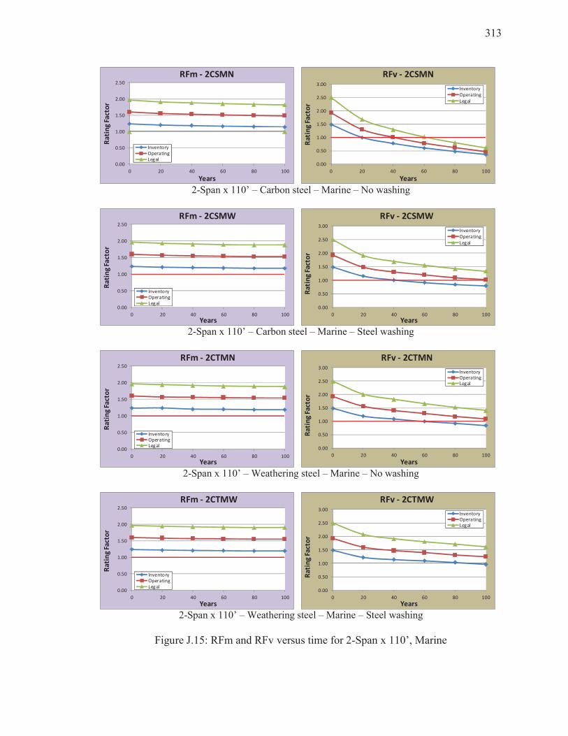
313
2-Span x 110’ – Carbon steel – Marine – No washing
2-Span x 110’ – Carbon steel – Marine – Steel washing
2-Span x 110’ – Weathering steel – Marine – No washing
2-Span x 110’ – Weathering steel – Marine – Steel washing
Figure J.15: RFm and RFv versus time for 2-Span x 110’, Marine
0.00
0.50
1.00
1.50
2.00
2.50
0 20 40 60 80 100
Ra
tin
g F
act
or
Years
RFm - 2CSMN
InventoryOperatingLegal
0.00
0.50
1.00
1.50
2.00
2.50
3.00
0 20 40 60 80 100
Ra
tin
g F
act
or
Years
RFv - 2CSMN
Inventory
Operating
Legal
0.00
0.50
1.00
1.50
2.00
2.50
0 20 40 60 80 100
Ra
tin
g F
act
or
Years
RFm - 2CSMW
InventoryOperatingLegal
0.00
0.50
1.00
1.50
2.00
2.50
3.00
0 20 40 60 80 100
Ra
tin
g F
act
or
Years
RFv - 2CSMW
Inventory
Operating
Legal
0.00
0.50
1.00
1.50
2.00
2.50
0 20 40 60 80 100
Ra
tin
g F
act
or
Years
RFm - 2CTMN
InventoryOperatingLegal
0.00
0.50
1.00
1.50
2.00
2.50
3.00
0 20 40 60 80 100
Ra
tin
g F
act
or
Years
RFv - 2CTMN
InventoryOperatingLegal
0.00
0.50
1.00
1.50
2.00
2.50
0 20 40 60 80 100
Ra
tin
g F
act
or
Years
RFm - 2CTMW
InventoryOperatingLegal
0.00
0.50
1.00
1.50
2.00
2.50
3.00
0 20 40 60 80 100
Ra
tin
g F
act
or
Years
RFv - 2CTMW
InventoryOperatingLegal

314
2-Span x 130’ – Carbon steel – Marine – No washing
2-Span x 130’ – Carbon steel – Marine – Steel washing
2-Span x 130’ – Weathering steel – Marine – No washing
2-Span x 130’ – Weathering steel – Marine – Steel washing
Figure J.16: RFm and RFv versus time for 2-Span x 130’, Marine
0.00
0.50
1.00
1.50
2.00
0 20 40 60 80 100
Ra
tin
g F
act
or
Years
RFm - 2DSMN
Inventory
Operating
Legal0.00
1.00
2.00
3.00
4.00
0 20 40 60 80 100
Ra
tin
g F
act
or
Years
RFv - 2DSMN
InventoryOperatingLegal
0.00
0.50
1.00
1.50
2.00
0 20 40 60 80 100
Ra
tin
g F
act
or
Years
RFm - 2DSMW
InventoryOperatingLegal 0.00
0.50
1.00
1.50
2.00
2.50
3.00
3.50
0 20 40 60 80 100R
ati
ng
Fa
cto
r
Years
RFv - 2DSMW
Inventory
Operating
Legal
0.00
0.50
1.00
1.50
2.00
2.50
0 20 40 60 80 100
Ra
tin
g F
act
or
Years
RFm - 2DTMN
InventoryOperatingLegal
0.00
0.50
1.00
1.50
2.00
2.50
3.00
3.50
0 20 40 60 80 100
Ra
tin
g F
act
or
Years
RFv - 2DTMN
Inventory
Operating
Legal
0.00
0.50
1.00
1.50
2.00
2.50
0 20 40 60 80 100
Ra
tin
g F
act
or
Years
RFm - 2DTMW
InventoryOperatingLegal
0.00
0.50
1.00
1.50
2.00
2.50
3.00
3.50
0 20 40 60 80 100
Ra
tin
g F
act
or
Years
RFv - 2DTMW
Inventory
Operating
Legal
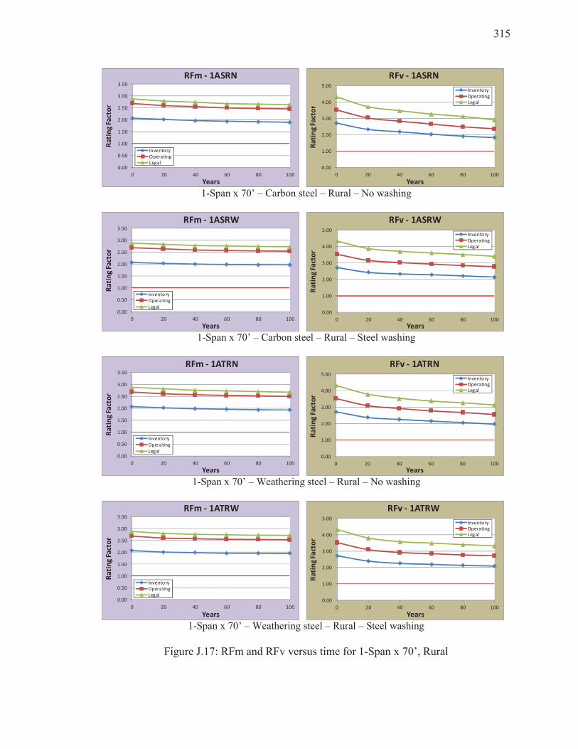
315
1-Span x 70’ – Carbon steel – Rural – No washing
1-Span x 70’ – Carbon steel – Rural – Steel washing
1-Span x 70’ – Weathering steel – Rural – No washing
1-Span x 70’ – Weathering steel – Rural – Steel washing
Figure J.17: RFm and RFv versus time for 1-Span x 70’, Rural
0.00
0.50
1.00
1.50
2.00
2.50
3.00
3.50
0 20 40 60 80 100
Ra
tin
g F
act
or
Years
RFm - 1ASRN
InventoryOperatingLegal
0.00
1.00
2.00
3.00
4.00
5.00
0 20 40 60 80 100
Ra
tin
g F
act
or
Years
RFv - 1ASRN
InventoryOperatingLegal
0.00
0.50
1.00
1.50
2.00
2.50
3.00
3.50
0 20 40 60 80 100
Ra
tin
g F
act
or
Years
RFm - 1ASRW
Inventory
Operating
Legal0.00
1.00
2.00
3.00
4.00
5.00
0 20 40 60 80 100R
ati
ng
Fa
cto
r
Years
RFv - 1ASRW
InventoryOperatingLegal
0.00
0.50
1.00
1.50
2.00
2.50
3.00
3.50
0 20 40 60 80 100
Ra
tin
g F
act
or
Years
RFm - 1ATRN
Inventory
Operating
Legal0.00
1.00
2.00
3.00
4.00
5.00
0 20 40 60 80 100
Ra
tin
g F
act
or
Years
RFv - 1ATRN
InventoryOperatingLegal
0.00
0.50
1.00
1.50
2.00
2.50
3.00
3.50
0 20 40 60 80 100
Ra
tin
g F
act
or
Years
RFm - 1ATRW
InventoryOperatingLegal
0.00
1.00
2.00
3.00
4.00
5.00
0 20 40 60 80 100
Ra
tin
g F
act
or
Years
RFv - 1ATRW
InventoryOperatingLegal
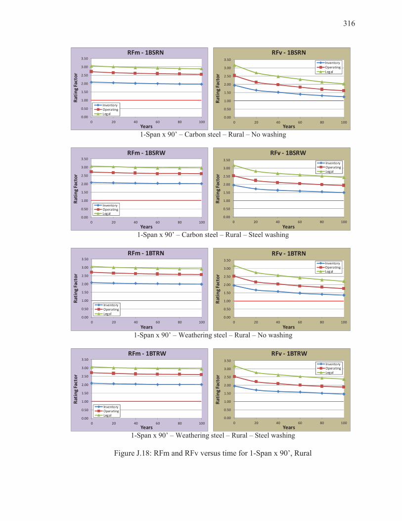
316
1-Span x 90’ – Carbon steel – Rural – No washing
1-Span x 90’ – Carbon steel – Rural – Steel washing
1-Span x 90’ – Weathering steel – Rural – No washing
1-Span x 90’ – Weathering steel – Rural – Steel washing
Figure J.18: RFm and RFv versus time for 1-Span x 90’, Rural
0.00
0.50
1.00
1.50
2.00
2.50
3.00
3.50
0 20 40 60 80 100
Ra
tin
g F
act
or
Years
RFm - 1BSRN
Inventory
Operating
Legal0.00
0.50
1.00
1.50
2.00
2.50
3.00
3.50
0 20 40 60 80 100
Ra
tin
g F
act
or
Years
RFv - 1BSRN
Inventory
Operating
Legal
0.00
0.50
1.00
1.50
2.00
2.50
3.00
3.50
0 20 40 60 80 100
Ra
tin
g F
act
or
Years
RFm - 1BSRW
InventoryOperatingLegal
0.00
0.50
1.00
1.50
2.00
2.50
3.00
3.50
0 20 40 60 80 100R
ati
ng
Fa
cto
r
Years
RFv - 1BSRW
InventoryOperatingLegal
0.00
0.50
1.00
1.50
2.00
2.50
3.00
3.50
0 20 40 60 80 100
Ra
tin
g F
act
or
Years
RFm - 1BTRN
Inventory
Operating
Legal0.00
0.50
1.00
1.50
2.00
2.50
3.00
3.50
0 20 40 60 80 100
Ra
tin
g F
act
or
Years
RFv - 1BTRN
InventoryOperatingLegal
0.00
0.50
1.00
1.50
2.00
2.50
3.00
3.50
0 20 40 60 80 100
Ra
tin
g F
act
or
Years
RFm - 1BTRW
InventoryOperatingLegal
0.00
0.50
1.00
1.50
2.00
2.50
3.00
3.50
0 20 40 60 80 100
Ra
tin
g F
act
or
Years
RFv - 1BTRW
InventoryOperatingLegal
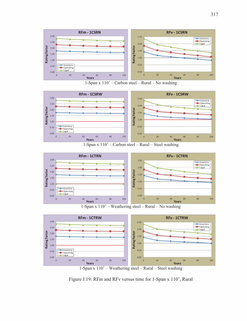
317
1-Span x 110’ – Carbon steel – Rural – No washing
1-Span x 110’ – Carbon steel – Rural – Steel washing
1-Span x 110’ – Weathering steel – Rural – No washing
1-Span x 110’ – Weathering steel – Rural – Steel washing
Figure J.19: RFm and RFv versus time for 1-Span x 110’, Rural
0.00
0.50
1.00
1.50
2.00
2.50
3.00
0 20 40 60 80 100
Ra
tin
g F
act
or
Years
RFm - 1CSRN
InventoryOperatingLegal
0.00
0.50
1.00
1.50
2.00
2.50
0 20 40 60 80 100
Ra
tin
g F
act
or
Years
RFv - 1CSRN
InventoryOperatingLegal
0.00
0.50
1.00
1.50
2.00
2.50
3.00
0 20 40 60 80 100
Ra
tin
g F
act
or
Years
RFm - 1CSRW
InventoryOperatingLegal
0.00
0.50
1.00
1.50
2.00
2.50
0 20 40 60 80 100R
ati
ng
Fa
cto
r
Years
RFv - 1CSRW
InventoryOperatingLegal
0.00
0.50
1.00
1.50
2.00
2.50
3.00
0 20 40 60 80 100
Ra
tin
g F
act
or
Years
RFm - 1CTRN
InventoryOperatingLegal
0.00
0.50
1.00
1.50
2.00
2.50
0 20 40 60 80 100
Ra
tin
g F
act
or
Years
RFv - 1CTRN
InventoryOperatingLegal
0.00
0.50
1.00
1.50
2.00
2.50
3.00
0 20 40 60 80 100
Ra
tin
g F
act
or
Years
RFm - 1CTRW
InventoryOperatingLegal
0.00
0.50
1.00
1.50
2.00
2.50
0 20 40 60 80 100
Ra
tin
g F
act
or
Years
RFv - 1CTRW
Inventory
Operating
Legal
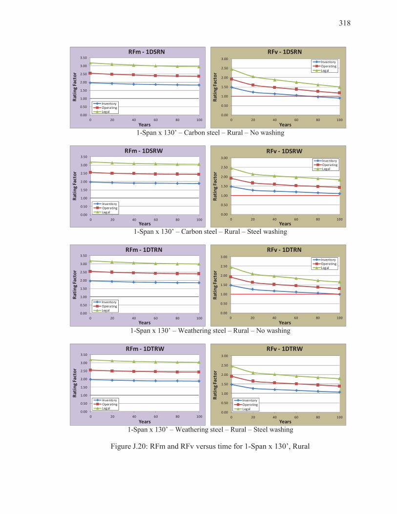
318
1-Span x 130’ – Carbon steel – Rural – No washing
1-Span x 130’ – Carbon steel – Rural – Steel washing
1-Span x 130’ – Weathering steel – Rural – No washing
1-Span x 130’ – Weathering steel – Rural – Steel washing
Figure J.20: RFm and RFv versus time for 1-Span x 130’, Rural
0.00
0.50
1.00
1.50
2.00
2.50
3.00
3.50
0 20 40 60 80 100
Ra
tin
g F
act
or
Years
RFm - 1DSRN
InventoryOperatingLegal
0.00
0.50
1.00
1.50
2.00
2.50
3.00
0 20 40 60 80 100
Ra
tin
g F
act
or
Years
RFv - 1DSRN
Inventory
Operating
Legal
0.00
0.50
1.00
1.50
2.00
2.50
3.00
3.50
0 20 40 60 80 100
Ra
tin
g F
act
or
Years
RFm - 1DSRW
InventoryOperatingLegal
0.00
0.50
1.00
1.50
2.00
2.50
3.00
0 20 40 60 80 100R
ati
ng
Fa
cto
r
Years
RFv - 1DSRW
InventoryOperatingLegal
0.00
0.50
1.00
1.50
2.00
2.50
3.00
3.50
0 20 40 60 80 100
Ra
tin
g F
act
or
Years
RFm - 1DTRN
InventoryOperatingLegal
0.00
0.50
1.00
1.50
2.00
2.50
3.00
0 20 40 60 80 100
Ra
tin
g F
act
or
Years
RFv - 1DTRN
InventoryOperatingLegal
0.00
0.50
1.00
1.50
2.00
2.50
3.00
3.50
0 20 40 60 80 100
Ra
tin
g F
act
or
Years
RFm - 1DTRW
InventoryOperatingLegal
0.00
0.50
1.00
1.50
2.00
2.50
3.00
0 20 40 60 80 100
Ra
tin
g F
act
or
Years
RFv - 1DTRW
Inventory
Operating
Legal
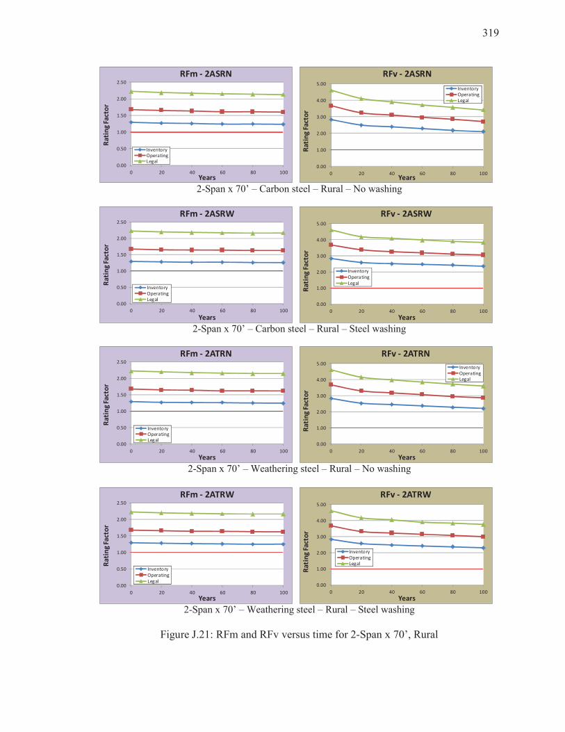
319
2-Span x 70’ – Carbon steel – Rural – No washing
2-Span x 70’ – Carbon steel – Rural – Steel washing
2-Span x 70’ – Weathering steel – Rural – No washing
2-Span x 70’ – Weathering steel – Rural – Steel washing
Figure J.21: RFm and RFv versus time for 2-Span x 70’, Rural
0.00
0.50
1.00
1.50
2.00
2.50
0 20 40 60 80 100
Ra
tin
g F
act
or
Years
RFm - 2ASRN
InventoryOperatingLegal
0.00
1.00
2.00
3.00
4.00
5.00
0 20 40 60 80 100
Ra
tin
g F
act
or
Years
RFv - 2ASRN
InventoryOperatingLegal
0.00
0.50
1.00
1.50
2.00
2.50
0 20 40 60 80 100
Ra
tin
g F
act
or
Years
RFm - 2ASRW
InventoryOperatingLegal
0.00
1.00
2.00
3.00
4.00
5.00
0 20 40 60 80 100R
ati
ng
Fa
cto
r
Years
RFv - 2ASRW
Inventory
Operating
Legal
0.00
0.50
1.00
1.50
2.00
2.50
0 20 40 60 80 100
Ra
tin
g F
act
or
Years
RFm - 2ATRN
InventoryOperatingLegal
0.00
1.00
2.00
3.00
4.00
5.00
0 20 40 60 80 100
Ra
tin
g F
act
or
Years
RFv - 2ATRN
InventoryOperatingLegal
0.00
0.50
1.00
1.50
2.00
2.50
0 20 40 60 80 100
Ra
tin
g F
act
or
Years
RFm - 2ATRW
Inventory
Operating
Legal0.00
1.00
2.00
3.00
4.00
5.00
0 20 40 60 80 100
Ra
tin
g F
act
or
Years
RFv - 2ATRW
InventoryOperatingLegal
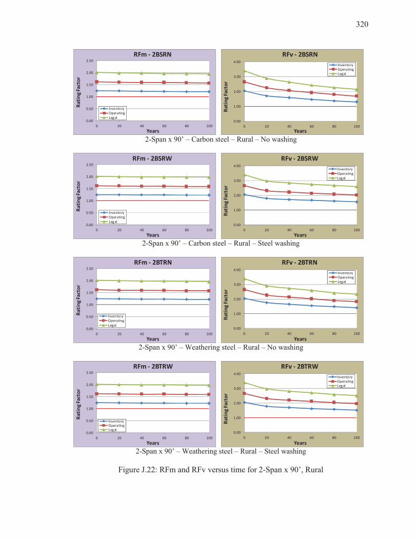
320
2-Span x 90’ – Carbon steel – Rural – No washing
2-Span x 90’ – Carbon steel – Rural – Steel washing
2-Span x 90’ – Weathering steel – Rural – No washing
2-Span x 90’ – Weathering steel – Rural – Steel washing
Figure J.22: RFm and RFv versus time for 2-Span x 90’, Rural
0.00
0.50
1.00
1.50
2.00
2.50
0 20 40 60 80 100
Ra
tin
g F
act
or
Years
RFm - 2BSRN
Inventory
Operating
Legal0.00
1.00
2.00
3.00
4.00
0 20 40 60 80 100
Ra
tin
g F
act
or
Years
RFv - 2BSRN
InventoryOperatingLegal
0.00
0.50
1.00
1.50
2.00
2.50
0 20 40 60 80 100
Ra
tin
g F
act
or
Years
RFm - 2BSRW
Inventory
Operating
Legal0.00
1.00
2.00
3.00
4.00
0 20 40 60 80 100R
ati
ng
Fa
cto
r
Years
RFv - 2BSRW
Inventory
Operating
Legal
0.00
0.50
1.00
1.50
2.00
2.50
0 20 40 60 80 100
Ra
tin
g F
act
or
Years
RFm - 2BTRN
Inventory
Operating
Legal0.00
1.00
2.00
3.00
4.00
0 20 40 60 80 100
Ra
tin
g F
act
or
Years
RFv - 2BTRN
InventoryOperatingLegal
0.00
0.50
1.00
1.50
2.00
2.50
0 20 40 60 80 100
Ra
tin
g F
act
or
Years
RFm - 2BTRW
InventoryOperatingLegal
0.00
1.00
2.00
3.00
4.00
0 20 40 60 80 100
Ra
tin
g F
act
or
Years
RFv - 2BTRW
InventoryOperatingLegal

321
2-Span x 110’ – Carbon steel – Rural – No washing
2-Span x 110’ – Carbon steel – Rural – Steel washing
2-Span x 110’ – Weathering steel – Rural – No washing
2-Span x 110’ – Weathering steel – Rural – Steel washing
Figure J.23: RFm and RFv versus time for 2-Span x 110’, Rural
0.00
0.50
1.00
1.50
2.00
2.50
0 20 40 60 80 100
Ra
tin
g F
act
or
Years
RFm - 2CSRN
InventoryOperatingLegal
0.00
0.50
1.00
1.50
2.00
2.50
3.00
0 20 40 60 80 100
Ra
tin
g F
act
or
Years
RFv - 2CSRN
InventoryOperatingLegal
0.00
0.50
1.00
1.50
2.00
2.50
0 20 40 60 80 100
Ra
tin
g F
act
or
Years
RFm - 2CSRW
InventoryOperatingLegal
0.00
0.50
1.00
1.50
2.00
2.50
3.00
0 20 40 60 80 100R
ati
ng
Fa
cto
r
Years
RFv - 2CSRW
InventoryOperatingLegal
0.00
0.50
1.00
1.50
2.00
2.50
0 20 40 60 80 100
Ra
tin
g F
act
or
Years
RFm - 2CTRN
InventoryOperatingLegal
0.00
0.50
1.00
1.50
2.00
2.50
3.00
0 20 40 60 80 100
Ra
tin
g F
act
or
Years
RFv - 2CTRN
InventoryOperatingLegal
0.00
0.50
1.00
1.50
2.00
2.50
0 20 40 60 80 100
Ra
tin
g F
act
or
Years
RFm - 2CTRW
InventoryOperatingLegal
0.00
0.50
1.00
1.50
2.00
2.50
3.00
0 20 40 60 80 100
Ra
tin
g F
act
or
Years
RFv - 2CTRW
InventoryOperatingLegal
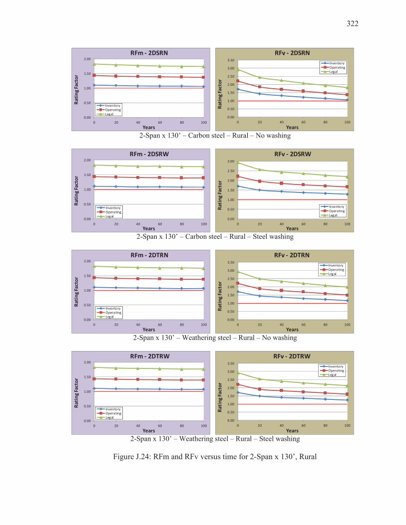
322
2-Span x 130’ – Carbon steel – Rural – No washing
2-Span x 130’ – Carbon steel – Rural – Steel washing
2-Span x 130’ – Weathering steel – Rural – No washing
2-Span x 130’ – Weathering steel – Rural – Steel washing
Figure J.24: RFm and RFv versus time for 2-Span x 130’, Rural
0.00
0.50
1.00
1.50
2.00
0 20 40 60 80 100
Ra
tin
g F
act
or
Years
RFm - 2DSRN
InventoryOperatingLegal
0.00
0.50
1.00
1.50
2.00
2.50
3.00
3.50
0 20 40 60 80 100
Ra
tin
g F
act
or
Years
RFv - 2DSRN
InventoryOperatingLegal
0.00
0.50
1.00
1.50
2.00
0 20 40 60 80 100
Ra
tin
g F
act
or
Years
RFm - 2DSRW
InventoryOperatingLegal
0.00
0.50
1.00
1.50
2.00
2.50
3.00
0 20 40 60 80 100R
ati
ng
Fa
cto
r
Years
RFv - 2DSRW
InventoryOperatingLegal
0.00
0.50
1.00
1.50
2.00
0 20 40 60 80 100
Ra
tin
g F
act
or
Years
RFm - 2DTRN
InventoryOperatingLegal
0.00
0.50
1.00
1.50
2.00
2.50
3.00
3.50
0 20 40 60 80 100
Ra
tin
g F
act
or
Years
RFv - 2DTRN
InventoryOperatingLegal
0.00
0.50
1.00
1.50
2.00
0 20 40 60 80 100
Ra
tin
g F
act
or
Years
RFm - 2DTRW
InventoryOperatingLegal
0.00
0.50
1.00
1.50
2.00
2.50
3.00
3.50
0 20 40 60 80 100
Ra
tin
g F
act
or
Years
RFv - 2DTRW
InventoryOperatingLegal

13
VITA
323
VITA
Luis M. Moran Yanez was born in Lima, Perú on December 16th, 1960. He received his
B.S. in Civil Engineering from the Pontifical Catholic University of Peru (Pontificia
Universidad Católica del Perú) in 1986 and his M.S. in Civil Engineering from the Imperial
College of Science and Technology - University of London, in London in 1991.